NBER WORKING PAPER SERIES

DYNAMIC TRADING STRATEGIES AND PORTFOLIO CHOICE

Ravi BansalMagnus Dahlquist

Campbell R. Harvey

Working Paper 10820http://www.nber.org/papers/w10820

NATIONAL BUREAU OF ECONOMIC RESEARCH1050 Massachusetts Avenue

Cambridge, MA 02138September 2004

The views expressed herein are those of the author(s) and not necessarily those of the National Bureau ofEconomic Research.

©2004 by Ravi Bansal, Magnus Dahlquist, and Campbell R. Harvey. All rights reserved. Short sections oftext, not to exceed two paragraphs, may be quoted without explicit permission provided that full credit,including © notice, is given to the source.

Dynamic Trading Strategies and Portfolio ChoiceRavi Bansal, Magnus Dahlquist, and Campbell R. HarveyNBER Working Paper No. 10820September 2004JEL No. G11, G12

ABSTRACT

Traditional mean-variance efficient portfolios do not capture the potential wealth creation

opportunities provided by predictability of asset returns. We propose a simple method for

constructing optimally managed portfolios that exploits the possibility that asset returns are

predictable. We implement these portfolios in both single and multi-period horizon settings. We

compare alternative portfolio strategies which include both buy-and-hold and fixed weight portfolios.

We find that managed portfolios can significantly improve the mean-variance trade-off, in particular,

for investors with investment horizons of three to five years. Also, in contrast to popular advice, we

show that the buy-and-hold strategy should be avoided.

Ravi BansalDepartment of EconomicsDuke UniversityDurham, NC 27708

Magnus DahlquistStockholm School of Economicsand Stockholm Institute for Financial ResearchStockholm, Swedenmagnus.dahlquist@sifr.org

Campbell R. HarveyFuqua School of BusinessDuke UniversityDurham, NC 27708-0120

1 Introduction

The choice of the optimal investment strategy is a core concern in financial economics.

Typical investment advice is to ‘invest for the long run,’ which usually means buy and

hold assets for a given horizon. What are the implications of such an investment strat-

egy? There are four important dimensions for the portfolio choice problem: the asset

menu, the investment horizon, the current state of the economy, and the investor’s risk

aversion. In this paper, we evaluate the impact of all these dimensions.

The traditional implementation of the portfolio choice problem involves a mean-

variance optimization over a set of asset expected returns, variances and covariances.

When these moments are measured as sample averages based on historical data, the

efficient portfolio weights are constant. That is, the investment weights are unaffected

by economic conditions and the only action required is to rebalance the assets each pe-

riod to achieve fixed weights. The possibility that asset returns are predictable creates

an opportunity to construct dynamic trading strategies which offer superior risk and

expected return trade-offs relative to standard portfolios. These managed portfolios

are impacted by economic conditions. We augment the asset menu to include the dy-

namic trades of the primitive assets based on variables that predict returns. As a result,

in our optimal portfolio, the investment weights change through time. We are able to

immediately compare the performance of the traditional strategy (fixed weights) to the

strategy that uses dynamic strategies (time-varying weights).

The idea of incorporating dynamic strategies into portfolio choice originates in

Hansen and Richard (1987). Recent research using these insights includes Bansal,

Hsieh, and Viswanathan (1993), Bansal and Harvey (1996), Ferson and Siegel (2001),

Cochrane (2001), and Brandt and Santa-Clara (2004). The basic idea is as follows. There

are two ways to solve the mean-variance portfolio choice problem when there is con-

ditioning information. The first is to specify the joint conditional distribution of the

asset returns and to solve for the optimal portfolio. An alternative method, proposed

in Hansen and Richard (1987), is to add dynamic strategies to the menu of assets, and

solve the much easier unconditional mean-variance problem. One limitation of previ-

ous research is that it has mostly focused on one-period portfolio problems.

The role of time-varying investment weights is most natural in the context of multi-

1

horizon asset allocation problems. A common piece of asset management advice is to

follow the buy-and-hold strategy. This strategy is equivalent to increasing the weight

in the winner stocks and decreasing the weight in the losing stocks. An alternative

strategy is the fixed-weight strategy. In this case, the investor always holds a fixed

fraction of his wealth in a particular asset. The rebalancing necessary to maintain fixed

weights has a contrarian flavor (i.e., selling the winners and buying the losers). The

key advantage to both these strategies is that they are easy to implement. However,

both of these strategies ignore information about the current state of the economy. Our

research goal is to contrast the performance of these strategies with a portfolio choice

method that incorporates dynamic trading strategies.

Our research makes three contributions. First, following Bansal and Harvey (1996),

we present a simplified method of solving the mean-variance portfolio problem that

incorporates conditioning information. We do this for both a single period and a long-

horizon portfolio problem. Second, we characterize the degree of predictability in asset

returns by comparing the performance of portfolio strategies that include or exclude

conditioning information. Third, we compare and contrast dynamic strategies with

both the fixed weights and buy-and-hold strategies over four popular portfolio choice

problems.

To highlight the importance of predictability in dynamic asset allocation, Campbell

and Viceira (1999) use a vector autoregression (VAR) approach. They use this structure

to address issues about optimal dynamic asset allocation for an infinite lived agent

who can rebalance each time period. Liu (2002) considers more parametric solutions

(derived numerically) to derive optimal portfolio weights. Our long-lived investors,

in contrast, design an optimal asset allocation plan at date t by trying to maximize the

utility over wealth for date t + h. They understand that returns are predictable hence

put fixed date t weights also on actively managed funds (i.e., dynamic trades) which

incorporate conditioning information and let their portfolio evolve until date t + h.

Our approach answers the question: at date t, what fraction of wealth should be put in

different assets given, (i) a horizon h, (ii) quadratic preferences for the terminal date,

(iii) access to actively managed funds, and (iv) the agent chooses not to actively change

the allocation after date t, though the actively managed funds are allowed to do so.

In other words, our investor is a passive investor who invests in actively managed

2

funds. The dynamic trading is done by the active managers—not directly by our in-

vestor. In this sense, our strategy is static from the perspective of the investor. We

suspect that this environment captures the opportunity set and behavior for a sizable

group of investors and hence is of considerable practical interest. The earlier paper

by Bekaert and Liu (2004) considers one-period ahead asset allocation with condition-

ing information, but does not entertain, as in our paper, multi-horizon asset allocation

problems.

Our results can be summarized as follows. First, investment in actively managed

(market timing) funds relative to traditional fixed weight strategy produces consider-

able economic gains. Hence, active funds can be of great benefit to investors. Second,

the traditional adage of buy-and-hold for long horizons is poor advice even compared

to the traditional fixed-weight investment strategy which incorporates no condition-

ing information. Our evidence is in line with Samuelson (1994) who also argues that

buy-and-hold may not necessarily be a good strategy. The strategy that incorporates

conditioning information performs the best. Third, we show that the economic gains

from using conditioning information increase with horizon of the portfolio allocation

decision. Fourth, we present an simplified approach to think about multi-horizon port-

folio choice which incorporates conditioning information.

The paper is organized as follows. In the second section we show how to construct

the unconditional mean-variance frontier which incorporates dynamic trading strate-

gies. We characterize the mean-variance frontier, discuss the portfolio choice problem

of a mean-variance investor, and consider restricted trading strategies. This section

also outlines a multi-horizon portfolio choice problem. The third section describes the

data and present evidence on predictive regressions. In the fourth section, we evaluate

different portfolio choice problems and measure the gains from dynamic trades. Some

conclusions are offered in the final section.

3

2 Dynamic Trading Strategies

2.1 Characterizing Mean-Variance Frontiers

The traditional approach to mean-variance portfolio choice solves for fixed portfolio

weights of returns, and ignores the fact that an investor can potentially rebalance their

portfolio in an dynamic manner based on information available at date t. However, it

makes sense that portfolio weights might change through time as the changes in the

economic environment can alter the distribution of returns. The traditional approach

can fail to exploit the potential benefits of predictability of returns (and the second

moment matrix) in forming portfolios.

Predictability of returns and/or of their second moments creates new investment

opportunities for the investor. These new opportunities are based on trading strategies

that exploit the predictability of the returns. For example, if a rise in the dividend-yield

suggests that future equity returns will be higher, then buying more equity as the div-

idend yield rises can create superior portfolio performance relative to the traditional

approach. That is, by exploiting this predictability one can potentially have a “bigger”

unconditional (i.e., average) investment opportunity set relative to the one that ignores

this predictability. One may also want to evaluate the conditional opportunity set: the

mean variance opportunity set for a given value for the dividend-yield and other pre-

dictive variables that determine the distribution of returns. Of course, if returns are

i.i.d. then the incorporation of conditioning information variables will not provide a

bigger investment opportunity set.

How can one characterize the conditional and the unconditional mean-variance

opportunities? Hansen and Richard (1987) provide a simple characterization of these

mean-variance frontiers. Both these frontiers exploit time-variation in the mean and

second moment matrix of returns. The unconditional frontier includes both basis as-

sets and dynamic strategies. This unconditional frontier is the optimal frontier in the

sense that it provides the best risk-return trade off among the set of all dynamic trades

that are feasible for an investor. Further, the unconditional frontier and the conditional

frontier for a given collection of returns can be characterized by two specific portfolios

discussed below. These two portfolios exploit the predictability in the mean and the

4

variance-covariance matrix of returns that is important for a mean-variance investor.

The ability to characterize the mean variance set, both conditionally and uncondition-

ally, with the same set of two specific portfolios makes their approach attractive to use.

To describe the Hansen and Richard (1987) formulation of the conditional and un-

conditional frontiers, consider the following vectors. Let Rt+1 denote a K + 1 vector of

gross returns between t and t+1. The first element in Rt+1 is R0,t+1, and other elements

in Rt+1 are Ri,t+1 (i 6= 0). Next, let Xt+1 denote a K vector of excess returns with a typi-

cal element being Xi,t+1 = Ri,t+1 −R0,t+1. The normalizing asset with return R0,t+1 can

be any of the K + 1 assets. Further, we will refer to R as the entire set of gross returns

and X as the set of all potential excess returns.

Hansen and Richard (1987) characterize the investment opportunity conditionally

(that is, the relevant opportunity set at a given point in time, or for a given state), and

also characterize it on average (that is, unconditionally, or on average across states). An

important feature is that the conditional and unconditional frontiers are characterized

by the same two dynamic trade-based payoffs R∗t+1 ∈ R and X∗

t+1 ∈ X.

The unit-cost payoff R∗t+1 is on the conditional mean variance frontier, and has the

unique property that it is has the smallest noncentral conditional second moment (i.e.,

global minimum second noncentral moment return). It can be derived as the solutions

to the following problem:

minΛt

Et

(R2

t+1

), (1)

where Et denotes expectations conditional on information at date t and Λt is a vector

of weights on the basis assets. The optimal portfolio R∗t+1 can be obtained by exploiting

the first-order conditions associated with problem (1):

Et

(R∗

t+1Xt+1

)= 0, (2)

which implies that the dynamic portfolio weights satisfy

ΛR∗

t = −Et

(Xt+1X

′t+1

)−1 Et (Xt+1R0,t+1) . (3)

The zero-cost payoff X∗t+1 has the unique property that it has the largest conditional

mean to conditional standard deviation ratio (i.e., conditional Sharpe ratio), and Hansen

5

and Richard (1987) show that X∗t+1 can be obtained by exploiting

Et

(X∗

t+1Xt+1

)= Et (Xt+1) , (4)

which implies that the dynamic portfolio weights, ΛX∗t satisfy

ΛX∗

t = Et

(Xt+1X

′t+1

)−1 Et (Xt+1) . (5)

Note that all the portfolio weights are dynamic and depend on the first two conditional

moments of the returns.

In section 2.2, we will explore the mean-variance portfolio choice problem. How-

ever, it is important to note that while the expressions for ΛR∗t and ΛX∗

t are straight-

forward, the solutions are complicated because it is necessary to specify both the con-

ditional first and second moments of the asset returns. In section 2.3, we propose a

simple method to avoid specifying these moments.

All returns can be decomposed into convenient pieces, for example return Ri,t+1,

can be stated as

Ri,t+1 = R∗t+1 + Ri,t+1 −R∗

t+1. (6)

To characterize the mean-variance frontier, consider the following decomposition of

the excess return

Ri,t+1 −R∗t+1 = wi,tX

∗t+1 + ηi,t+1, (7)

where wi,t is the conditional linear projection coefficient. Exploiting the orthogonal-

ity of excess returns with R∗t+1, and that Vart

(X∗

t+1

)= Et

(X∗

t+1

) [1− Et

(X∗

t+1

)], the

coefficient wi,t can be further simplified,

wi,t =Covt

(X∗

t+1, Ri,t+1 −R∗t+1

)Vart

(X∗

t+1

) =Et

(Ri,t+1 −R∗

t+1

)Et

(X∗

t+1

) . (8)

This property ensures that Et

(X∗

t+1ηi,t+1

)= 0 and Et (ηi,t+1) = 0.

Any return Ri,t+1 can be written as

Ri,t+1 = R∗t+1 + wi,tX

∗t+1 + ηi,t+1. (9)

The three pieces in the above decomposition are orthogonal to each other and the term

ηi,t+1 has a zero mean. Consequently, the conditional mean-variance frontier is simply

6

characterized by R∗t+1 and X∗

t+1, and entails no investment in the residual term ηi,t+1.

The collection of all returns with a conditional mean of ct are described by

R∗t+1 +

ct − Et

(R∗

t+1

)Et

(X∗

t+1

) X∗t+1 + ηt+1, (10)

where ηt+1 is an error term orthogonal to R∗t+1 and X∗

t+1. The minimum-variance unit-

cost payoff with a conditional mean of ct is then

R∗t+1 +

ct − Et

(R∗

t+1

)Et

(X∗

t+1

) X∗t+1. (11)

This follows from recognizing that ηt+1 is a zero-cost payoff that adds nothing to the

mean, but adds to the variance of the return with a target mean of ct.

2.2 Mean-Variance Portfolio Choice

Consider an investor that maximizes conditional mean-variance utility with risk aver-

sion parameter b:

Et (Rt+1)−b

2Vart (Rt+1) , (12)

subject to the constraint that this portfolio costs one dollar. All returns can be decom-

posed into R∗t+1, X∗

t+1, and ηt+1. As ηt+1 is a zero-cost portfolio that adds nothing to the

mean but adds to the variance, it follows that a mean-variance agent will invest only

in R∗t+1 and X∗

t+1. In particular, the investor’s choice is the solution to the problem

maxwt

Et

(R∗

t+1 + wtX∗t+1

)− b

2

[Vart

(R∗

t+1

)+ wt2Vart

(X∗

t+1

)+ 2wtCovt

(R∗

t+1, X∗t+1

)].

(13)

The investor’s optimal portfolio weight then satisfies

wt =Et

(X∗

t+1

)− bCovt

(R∗

t+1, X∗t+1

)bVart

(X∗

t+1

) =

[1 + bEt

(R∗

t+1

)]Et

(X∗

t+1

)bVart

(X∗

t+1

) . (14)

The key insight of Hansen and Richard (1987) is that the unconditional mean-

variance frontier (which includes both basis assets and managed portfolios) can also be

characterized by R∗t+1 and X∗

t+1. They show that the conditional moment restrictions

(2) and (4), via the law of iterated expectations, also hold unconditionally. The same

7

investor choosing a portfolio weight unconditionally, will hence choose w given by

w =E

(X∗

t+1

)− bCov

(R∗

t+1, X∗t+1

)bVar

(X∗

t+1

) =

[1 + bE

(R∗

t+1

)]E

(X∗

t+1

)bVar

(X∗

t+1

) . (15)

Even unconditionally, the investor’s optimal portfolio choice involves dynamic trading

as X∗t+1 and R∗

t+1 are payoffs constructed from dynamic trades and the solutions to X∗t+1

and R∗t+1 involve conditional expectations. The optimal portfolio weight between X∗

t+1

and R∗t+1 is fixed, but the weights given to individual securities in the portfolio are

dynamically changing. That is, even though w is fixed, ΛR∗t and ΛX∗

t are time-varying.

As a practical matter, even the optimal dynamic trades are hard to implement if the

set of random returns are large as it is hard to credibly model the first two conditional

moments of a large cross-section of assets.

2.3 Restricted Dynamic Trading Strategies

We now consider the practical solution to portfolio choice, by restricting the set of dy-

namic trading in particular ways. A consequence of restricting the dynamic trades

is that the implied dynamic portfolio weights will not be exploiting all the informa-

tion required to characterize the first two conditional moments. On the other hand, it

seems reasonable to believe that adding the restricted set of dynamic trading strategies

should bring us close to risk-expected return opportunities that obtain from exploiting

all information needed for the first two conditional moments.

Define the conditioning information as Zt, which is an L vector of variables known

at date t that help predict future returns. One element in Zt is a constant. Now let

Yt+1 denote the stacked KL vector of dynamic trading based payoffs, with a typical

element being Xi,t+1Zj,t. Note that each element of Yt+1 is a zero-cost payoff.1 The set

of portfolio holdings that are permitted in the restricted payoff structure are simply,

R0,t+1 + Λ′Yt+1, where Λ is a KL vector of constants that determines the portfolio

weights. While these weights are fixed, as the conditioning information changes the

weights on the K basis assets will change.

1Alternatively, it is possible to include squares of Zt or even cross-products of Zt.

8

Relative to the traditional mean-variance problem, the inclusion of the dynamic

trading based payoffs (or scaled excess returns) yield dynamic trades. The scaling

variables can include non-parametric functions of past returns (e.g., squared returns

motivated by ARCH and GARCH volatility models) allowing the investor to fully ex-

ploit all the predictability in the mean and the variance-covariance of returns. Intelli-

gent choice of the scaling variables can allow the investor to significantly improve the

unconditional investment opportunity set with a few scaling variables. One can also

interpret the implementation our ”restricted approach” as a traditional mean variance

approach but conducted over the augmented asset menu that includes the basis assets

and the scaled excess returns. We implement the characterization of the mean-variance

frontiers using the Hansen and Richard approach as it is easy to implement and affords

a simple link between the unconditional and conditional frontiers.

We construct the analogs of R∗t+1 and X∗

t+1, using the restricted trading strategies.

The restricted benchmark payoffs corresponding to R∗t+1 can be derived by exploiting

the equation analogous to equation (2):

E((R0,t+1 + Λ′Yt+1)Yt+1) = 0. (16)

It follows that the optimal parameter vector has to equal

ΛR∗= −E

(Yt+1Y

′t+1

)−1 E(Yt+1R0,t+1). (17)

Next we can use equation (4), to solve for the portfolio weights for X∗t+1.

E(X∗

t+1Yt+1

)= E (Yt+1) . (18)

Hence,

ΛX∗= E

(Yt+1Y

′t+1

)−1 E (Yt+1) . (19)

To characterize the unconditional mean-variance frontier, we now use the parameter

vectors ΛR∗ and ΛX∗ to construct the restricted analogs of R∗t+1 and X∗

t+1. There is a

critical difference between ΛR∗t in (2) and ΛX∗

t in (4) and the above ΛR∗ and ΛX∗—the

time subscripts on the weights.

In the original problem with the K basis assets, the weights that determine R∗t and

X∗t change through time as a function of the conditional means, variances and covari-

9

ances of the basis assets. In the above problem, the weights on the KL investments

(which include both the basis assets and the basis assets multiplied by the condition-

ing information) are constant. The key insight is that as a result of time variation in the

conditioning information the effective weights on the basis assets also change in this

setup. It is straightforward to also solve for the weights of a mean-variance investor

with a risk aversion parameter b as in the previous sub-section.

2.4 Multi-Horizon Portfolio Choice

2.4.1 Dynamic Portfolio Choice with Conditioning Information

The above analysis can be extended to consider mean-variance opportunity sets for

horizons longer than one period. For expositional ease we show our results for a two

period case; the case with longer horizons is a simple extension of the two period

analysis.

Consider the one-period dynamic trade Rd,t+1 = R0,t+1 + Zj,t(Ri,t+1 − R0,t+1). The

two period excess return if one were to invest γ dollars at date t in the portfolio is

γ (Rd,t+1Rd,t+2 −R0,t+1R0,t+2). This payoff costs zero dollars at date t and the excess

return is equal to

γZj,tR0,t+2(Ri,t+1 −R0,t+1) + γZj,t+1R0,t+1(Ri,t+2 −R0,t+2), (20)

where we have ignored the small cross product term γ2Zj,t(Ri,t+1−R0,t+1)Zj,t+1(Ri,t+2−R0,t+2). In other words, the two period excess return trade is essentially a dynamic

trade on a series of one period excess returns. This simple description helps interpret

our construct of the multi-horizon mean variance frontier discussed below.

The set of portfolio holdings that are permitted in the restricted payoff structure are

simply, R0,t+1R0,t+2 + Λ′2Yt,t+2, where Λ2 is a KL vector of constants, and a typical ele-

ment of Yt,t+2 is Rd,t+1Rd,t+2 −R0,t+1R0,t+2, as described above. Then we can construct

the global minimum second (noncentral) moment portfolio, R∗t,t+2 by solving:

E((R0,t+1R0,t+2 + Λ′2Yt,t+2)Yt,t+2) = 0, (21)

10

with

ΛR∗

2 = −E(Yt,t+2Y

′t,t+2

)−1 E(Yt,t+2R0,t+1R0,t+2), (22)

where the sub-script underscores that these parameters depend on the horizon under

construction. Analogously, to determine the zero cost payoff with the maximal Sharpe

ratio, we first set X∗t,t+2 = Λ′

2Yt,t+2, and the solution for Λ2 must satisfy

E((

Λ′2Yt,t+2

)Yt,t+2

)= E (Yt,t+2) . (23)

Hence,

ΛX∗

2 = E(Yt,t+2Y

′t,t+2

)−1 E (Yt,t+2) . (24)

The above analysis can be extended to any horizon h by constructing

R0,t+1R0,t+2 · · ·R0,t+h

and Yt,t+h with a typical element

Rd,t+1Rd,t+2 · · ·Rd,t+h −R0,t+1R0,t+2 · · ·R0,t+h.

The solutions for the analogs of R∗t+h and X∗

t+h can be constructed by solving for ΛR∗

h

and ΛX∗

h . Note that when h is one, then the problem coincides with the one period

problem. Further, given ΛR∗

h and ΛX∗

h , the mean-variance portfolio choice for a given

horizon follows the same logic as discussed in the one period case in section 2.2.

2.4.2 Alternative Long Horizon Trading Strategies

In addition to the above dynamic trades, we also consider two other trading strategies.

One is the classic buy-and-hold strategy. In this case, the agent invests at the initial

date in different assets and then holds this position to the end of the horizon. Hence,

the portfolio weights wi,t on a given asset evolves as

wi,t+1 = wi,tRi,t+1

Rp,t+1

. (25)

In a buy and hold strategy, the investor invests more in assets which have high gains

relative to the overall portfolio return. This feature of the buy-and-hold also implies

that at long horizons the portfolio becomes less balanced and may impose undue risks

11

on the investor due to lack of diversification. In computing the optimal buy-and-hold

strategy the choice variable is the initial portfolio weights—given this the evolution of

weights across time is governed by equation (25).

The third long run strategy is the fixed weight strategy in the basis assets. This

can be seen as a special case of the time-varying weight case where Zt only contains a

constant and no information variables. In this strategy, the investor’s rebalancing re-

sembles contrarian-like strategy. The investor buys more, in dollar terms, of the stocks

that perform relatively poorly and sells the winning stocks.2 This rebalancing ensures

that the portfolio weights are constant across time. To estimate the portfolio weights,

we need to estimate the starting weights and hold them fixed for the entire sample. In

contrast to the buy-and-hold, this strategy involves rebalancing every period. How-

ever, both the fixed-weight and the buy-and-hold strategies have the common feature

that they ignore all conditioning information.

3 Portfolio Choice Applications

3.1 Four Asset Allocation Problems

We consider four asset allocation problems which are detailed in Table 1. Problem I (la-

beled U.S. Equity/Fixed Income) considers the choice between Treasury Bills, Treasury

Bonds, and a U.S. equity portfolio represented by the S&P 500. Problem II (World Eq-

uity) considers allocation to a measure of a world market portfolio (exclusive the U.S.)

from MSCI in addition to Treasury Bills and the S&P 500. Problem III (U.S. Growth

and Value) considers the allocation between portfolios of growth and value stocks in

addition to Treasury Bills. Problem IV (U.S. Bonds) considers the allocation between

Treasury Bills, Treasury Bonds, and portfolios of corporate bonds and mortgages. All

problems consider real returns (nominal returns are adjusted for inflation). Note that

2This is only true if there is no leverage. For example, consider the case with one stock and oneriskless asset. Assuming that the fixed weight of the stock is 200%. If the initial wealth is $100. Theinvestor will borrow $100 to buy $200 of the stock. Assuming that the gross riskless return is 1 and thestock value goes to $300. The total wealth of the investor before rebalance is $200. For the stock weightto be 200%, the investor needs to borrow another $100 to buy additional $100 of the stock.

12

all asset returns (including Treasury Bills) are risky in real terms as there is inflation

uncertainty. The sample periods are determined by data availability as shown in the

table, and vary across the four problems.

Dynamic trading strategies are formed by conditional information variables. These

variables together with the actual returns on the above asset classes are described next.

In our set up, we solve for the optimal portfolio weights for investment in actively

managed funds. As such, we make no allowances for transactions costs. In practice, the

historical performance of the active managers would already reflect the transactions

costs and our method could be directly applied. However, in the following examples,

we create example active strategies which are presumed to be executed on futures with

low transactions costs.3

3.2 Summary Statistics and Predictability

Some summary statistics on the eight asset classes used for portfolio choice problems

are presented in Panel A of Table 2. The information variables that will be used to

form dynamic trading strategies are: the S&P 500 dividend yield (labeled Dividend

Yield), the Baa-Aaa yield spread (Spread), the difference of a 10-year Treasury and a

90-day Treasury bond yield (Slope), and the yield on the 90-day Treasury bill (Level).

The information variables are all lagged one month. The choice of the conditioning

variables is motivated by the research of Keim and Stambaugh (1986), Campbell (1987),

Fama and French (1988), and Harvey (1989). Information on data sources are given in

the table.

The average real returns on the S&P 500 and the MSCI World portfolios have been

70bp and 62bp per month, or about 8% per year, during their sample periods. The

average return on the T-bill portfolio has been about 12bp per month. The average

returns on the bond portfolios have been between 29bp and 40bp per month. The

average return on the portfolio of Value stocks has been about 90bp per month, 21bp

higher than the return on the portfolio of Growth stocks.

3Balduzzi and Lynch (1999) and Lynch and Balduzzi (2000) show, in a different setting, that pre-dictability of asset returns has large effects on rebalancing even in the presence of transaction costs.

13

The standard deviations of the equity portfolios have been between 3% and 4%

per month, or between 10% and 14% per year. The standard deviations of the bond

portfolios have been about half of the equity levels, that is, about 5% to 7% per year.

The lowest monthly returns on the equity portfolios (about -15%) were realized

in October 1987. The lowest and highest realized return on the bond portfolios were

during the turbulent period from 1979 to 1982 when the Federal Reserve experimented

with their monetary policy.

Panel B of Table 2 reports the correlations of the real returns and the conditional

information variables. The portfolios of corporate bonds and mortgages have a return

correlation of 86%. The correlation between the portfolios of growth and value stocks is

about 80%, lower than each of the two portfolios versus the S&P 500. The correlations

between the U.S. portfolios (equity and bonds) and the MSCI world excluding U.S.

portfolio are, except for the S&P 500, less than 60%. The correlations between the

equity and bond portfolios are about 20% to 30%. Among the information variables,

it is only the correlation between Level and Slope that is higher than 60%. Hence, the

information variables seem to measure different aspects of the state of the economy.

To gauge the potential gains from dynamic trades, we project the excess returns (the

returns on seven of the asset class portfolios over and above the return on the T-bill) on

a constant and each of the four information variables. [Recall that there are gains from

dynamic trading strategies if the information variables contain information on the first

two moments of the primitive assets. It is straightforward to show that predictability

of the excess returns is a sufficient condition for dynamic trading to be important for an

investor with mean-variance preferences.] Regression adjusted R-squares are reported

in Panel A of Table 2.

The adjusted R-squares are about 2% to 3%. The variables are jointly significant for

almost all asset classes (the p-values from a Wald test of jointly significant coefficients

are effectively 0%). Only the test on the Mortgage portfolio is marginally significant (a

p-value of 6%). Note that the Mortgage portfolio is the portfolio with fewest number of

observations. Overall, we find significant coefficients for the Dividend Yield, Spread,

and Level variables, especially in the predictability regression for the U.S. equity port-

folios. Further, the Slope variable is highly significant for the bond portfolios.

14

4 Evaluating Trading Strategies

4.1 One-Period Portfolio Choice

Table 3 highlights the importance of conditioning information in the context of static

portfolio choice. There is a substantial increase in the maximal Sharpe Ratio that one

can obtain by using the predictive variables. Column two provides the Sharpe ratio

based on the traditional mean variance analysis (fixed weights). The incorporation of

the conditioning information increases the Sharpe ratio by about 30% to 70% relative

to the traditional Sharpe ratios. For example, the monthly Sharpe ratio is 0.18 for the

U.S. Equity/Fixed Income problem where the weights are held constant and 0.27 when

dynamic trading strategies are introduced.

For various risk aversion levels there is substantial rise in utility associated with

using conditioning information. The gain in utility is reported in the last column of

the table – the certainty equivalent (CE) loss. For example, with a risk aversion param-

eter of 10 for the U.S Equity/Fixed Income allocation problem the increase in utility

corresponds to 20bp per month with a bootstrapped standard error of 11bp. Stated

differently, in order to achieve the same utility as the time-varying (dynamic) weight

investor, the fixed weight investor must have a 2.4% increment in annual return.

The standard errors in Table 3, and standard errors and confidence bands in sub-

sequent tables and figures, are generated in a parametric bootstrap. Returns and pre-

dictive variables are modeled as a VAR(1) where the residuals are re-sampled. The

portfolio choice is carried out using these generated data and used to construct the

statistic of interest. 3,000 replications were used in constructing standard errors and

(bias-adjusted) confidence bands.

The substantial increase in the mean-variance trade-off can also be seen in Figure 1,

which depicts 95% confidence bands for the unconditional mean –standard deviation

frontiers for fixed weight and time-varying (dynamic) weight strategies.

15

4.2 Multi-Horizon Portfolio Choice

The multi-horizon portfolio choice results are presented in Table 4. We evaluate the

importance of conditioning information in a multi-horizon context by comparing the

Sharpe ratios of the fixed weight strategy to the dynamic strategies for different hold-

ing periods.

The results in Table 4 show, in general, that conditioning information is more im-

portant in longer horizon portfolio problems. That is for a given horizon, the relative

ratio (ratio of dynamic strategy’s Sharpe ratio to the fixed weight strategy’s Sharpe

ratio) is larger at longer horizons for most of the portfolio allocation problems.

We also report the confidence interval for long-horizon risk return trade-offs (i.e.,

for the Sharpe ratio of X∗). In almost all cases, the 95% confidence interval lie above

the Sharpe ratio of the fixed weight strategy, indicating that increases in Sharpe ratios

due to dynamic strategies are statistically significant.

A comparison of the various portfolio choices also shows that the biggest impact of

conditioning information is in the context of the U.S. Bonds allocation. The addition of

conditioning information more than doubles the amount of expected return for a given

level of risk in each of the multiperiod scenarios. In the five-year horizon, the Sharpe

ratio of the dynamic strategy is almost four times greater than the fixed-weight Sharpe

ratio.

To further evaluate the importance of conditioning information we also report the

utility level for different horizons, risk aversion, and alternative portfolio choices in

Table 5. The utility level from the restricted dynamic multi-horizon portfolio choice

dominates the traditional fixed weight allocation prescriptions in almost all cases. In

many cases, the gain in utility is more pronounced at longer horizons (i.e., 3-5 years).

Consistent with Table 4, the largest differences are found with the U.S. Bonds choice

problem.

The bootstrap standard errors reveal that the utility gains are most significant for

domestic equity portfolios. For example, in the U.S. Equity/Fixed Income and the

Growth/Value portfolios, the gains are more than two standard errors from zero in 29

of 30 cases for the 2–4 year holding horizons. The significance levels are the weakest

16

for the international equity portfolios – which also has a much shorter sample than the

domestic equity portfolios. The utility gains for the bond portfolios also suffer from a

shorter sample. The most significant utility gains are for shorter horizon portfolios (4

of 5 cases for the one-year horizon). In the 2-4 year holding periods, the utility gains

are always more than one standard error from zero.

4.3 Fixed weight and buy-and-hold

In Table 6, we compare two alternative long-horizon portfolio choices; the fixed weight

portfolio at different horizons and a buy and hold strategy. We restrict our attention to

the U.S. Equity/Fixed Income allocation problem.4 Portfolio weights for an asset class

are restricted to be between 0% and 100%.5

Table 5 showed that dynamic strategies are superior to the fixed weight strate-

gies. Table 6 shows that fixed weight strategies do better than buy-and-hold strategies.

However, the difference between fixed weight and buy and hold is small. Note that the

utility differences reported in Table 6 are total differences over the investment horizon

whereas Table 5 reported monthly gains. Nevertheless, for the portfolios in the 2–5

year horizon, the fixed weight strategy often produces significantly more utility than

the buy-and-hold strategy. In this comparison, the largest and most significant differ-

ences are found for the investor with low risk aversion and with the longest horizon.

For a given risk aversion and horizon, Table 6 shows that the utility from fixed

weights is higher than that of buy and hold for all portfolio problems. The intuition for

this is simply that buy and hold leads to lack of diversification across time. Longer the

horizon, the greater is the relative loss in utility—this again, is due to the poor diver-

sification properties of the buy-and-hold strategy which gets worse with horizon. Our

estimation (not reported) shows that the initial weight for the buy and hold strategy is

lower than the weight in the fixed-weight strategy. Given the structure of the evolution

of the portfolio weights for buy-and-hold, the weight to the highest mean return asset

increases with time.4The results for the other portfolio choice problems are available on request.5The qualitative results are not sensitive to the imposed short sales restrictions.

17

5 Conclusions

Portfolio choice with conditioning information usually involves specifying the joint

conditional distribution of asset returns, extracting the conditional means, covariances

and variances and optimizing every period. Following Hansen and Richard (1987),

we offer a simple alternative. By adding the conditioning information directly to the

asset menu (by scaling returns by lagged information variables), one can solve the

unconditional mean-variance problem and obtain a single set of weights. As the infor-

mation variable change through time, the effective weights on the basis assets change.

The addition of these scaled returns, or dynamic trading strategies, makes conditional

portfolio selection straightforward.

Our paper solves the portfolio problem of the investor who wants the benefits asso-

ciated with incorporating conditioning information, but would prefer to delegate the

dynamic trading to active managers.

In addition to operationalizing the conditional portfolio selection problem, our pa-

per implements the selection problem in both single and multi-period investment hori-

zons. We are able to compare three different strategies: the dynamic strategy resulting

from adding scaled returns to the selection problem, fixed weight traditional mean-

variance selection, and the popular buy and hold strategy. We study four popular

portfolio choice problems.

Our results are as follows. Conditioning information is important. Even with low

levels of predictability, there is a substantial loss in opportunity when fixed-weight

strategies (which assume no predictability) are implemented relative to the dynamic

portfolio strategies that incorporate conditioning information. The popular buy-and-

hold strategy performs even worse than the fixed-weight strategy. The buy and hold is

a particularly poor strategy for longer-horizon investment decisions. The intuition is

that the buy and hold leads to substantially undiversified portfolios in the long-term.

Contrary to popular advice, the buy-and-hold strategy should be avoided.

18

References

Balduzzi, Pierluigi, and Anthony Lynch, 1999, Transaction Costs and Predictability:Some Utility Cost Calulations, Journal of Financial Economics 52, 47–78.

Bansal, Ravi, and Campbell R. Harvey, 1996, Performance Evaluation in the Presenceof Dynamic Trading Strategies, Working Paper, Duke University.

Bansal, Ravi, David A. Hsieh, and S. Viswanathan, 1993, A New Approach to Interna-tional Arbitrage Pricing, Journal of Finance 48, 1719–1747.

Bekaert, Geert, and Jun Liu, 2004, Conditioning Information and Variance Bounds onPricing Kernels, Review of Financial Studies 17, 339–378.

Brandt, Michael W., and Pedro Santa-Clara, 2004, Dynamic Portfolio Selection by Aug-menting the Asset Space, Working Paper, Duke University.

Campbell, John Y., 1987, Stock Returns and the Term Structure, Journal of Financial Eco-nomics 18, 373–399.

Campbell, John Y., and Luis M. Viceira, 1999, Consumption and Portfolio DecisionsWhen Expected Returns are Time Varying, Quarterly Journal of Economics 114, 433–495.

Cochrane, John H., 2001, Asset Pricing. (Princeton University Press, Princeton).

Fama, Eugene F., and Kenneth R. French, 1988, Dividend Yields and Expected StockReturns, Journal of Financial Economics 22, 3–26.

Ferson, Wayne E., and Andrew F. Siegel, 2001, The Efficient Use of Conditioning Infor-mation in Portfolios, Journal of Finance 56, 967–982.

Hansen, Lars Peter, and Scott F. Richard, 1987, The Role of Conditioning Informationin Deducing Testable Restrictions Implied by Dynamic Asset Pricing Models, Econo-metrica 55, 587–613.

Harvey, Campbell R., 1989, Time-Varying Conditional Covariances in Tests of AssetPricing Models, Journal of Financial Economics 24, 289–317.

Keim, Donald B., and Robert F. Stambaugh, 1986, Predicting Returns in the Stock andBond Markets, Journal of Financial Economics 17, 357–390.

Liu, Jun, 2002, Portfolio Selection in Stochastic Environments, Working Paper, UCLA.

Lynch, Anthony, and Pierluigi Balduzzi, 2000, Transaction Costs and Predictability:The Impact on Rebalancing Rules and Behavior, Journal of Finance 55, 2285–2309.

Samuelson, Paul A., 1994, The Long-Term Case for Equities, Journal of Portfolio Manage-ment 21, 15–24.

19

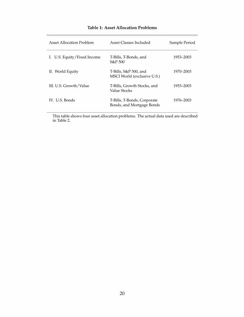
Table 1: Asset Allocation Problems

Asset Allocation Problem Asset Classes Included Sample Period

I. U.S. Equity/Fixed Income T-Bills, T-Bonds, and 1953–2003S&P 500

II. World Equity T-Bills, S&P 500, and 1970–2003MSCI World (exclusive U.S.)

III. U.S. Growth/Value T-Bills, Growth Stocks, and 1953–2003Value Stocks

IV. U.S. Bonds T-Bills, T-Bonds, Corporate 1976–2003Bonds, and Mortgage Bonds

This table shows four asset allocation problems. The actual data used are describedin Table 2.

20

Tabl

e2:

Sum

mar

ySt

atis

tics

ofR

ealR

etur

nsan

dC

ondi

tion

alIn

form

atio

nV

aria

bles

Cor

rela

tion

sIn

clus

ion

Dat

eM

ean

Stan

dard

Dev

iati

onA

djus

ted

R-s

quar

eT

1.2.

3.4.

5.6.

7.8.

Pane

lA.R

ealR

etur

ns

1.T-

Bills

53-0

50.

120.

24—

603

1.00

2.T-

Bond

s53

-05

0.29

2.24

1.98

603

0.36

1.00

3.S&

P50

053

-05

0.70

3.45

2.70

603

0.22

0.21

1.00

4.M

SCIW

orld

70-0

10.

624.

002.

8740

30.

330.

250.

611.

005.

Gro

wth

Stoc

ks53

-05

0.69

3.76

2.87

603

0.21

0.19

0.97

0.59

1.00

6.V

alue

Stoc

ks53

-05

0.90

3.76

2.56

603

0.21

0.16

0.87

0.53

0.79

1.00

7.C

orpo

rate

Bond

s53

-05

0.30

1.86

2.82

603

0.34

0.90

0.28

0.24

0.25

0.25

1.00

8.M

ortg

age

Bond

s76

-01

0.40

1.55

3.56

331

0.41

0.81

0.26

0.22

0.23

0.23

0.86

1.00

Pane

lB.C

ondi

tion

alIn

form

atio

nV

aria

bles

1.D

ivid

end

Yiel

d53

-05

3.48

1.17

—60

31.

002.

Spre

ad53

-05

0.95

0.42

—60

30.

401.

003.

Slop

e53

-05

1.03

1.30

—60

3-0

.18

0.11

1.00

4.Le

vel

53-0

55.

613.

11—

603

0.43

0.58

-0.4

91.

00

This

tabl

epr

esen

tssu

mm

ary

stat

isti

csof

mon

thly

real

dolla

rre

turn

sfo

rei

ghta

sset

clas

ses

from

incl

usio

nda

teto

July

2003

(Pan

elA

),an

dco

ndit

ioni

ngin

form

atio

nva

riab

les

from

May

1953

toJu

ly20

03(P

anel

B).T

heS&

P50

0an

dM

SCIW

orld

(exc

lusi

veU

.S.)

port

folio

sar

eta

ken

from

Dat

astr

eam

.The

Val

uean

dG

row

thpo

rtfo

lios

upto

Dec

embe

r200

2ar

eco

llect

edfr

omth

ew

ebsi

teof

Ken

neth

Fren

ch.O

bser

vati

ons

onth

eV

alue

and

Gro

wth

port

folio

sin

2003

are

from

Wils

hire

.T-B

ill,T

-Bon

d,an

dC

orpo

rate

Bond

port

folio

sar

efr

omIb

bots

onA

ssoc

iate

s.Th

eM

ortg

age

port

folio

isfr

omM

erri

llLy

nch.

All

port

folio

retu

rns

are

orig

inal

lyin

nom

inal

term

s,bu

tthe

yar

ead

just

edfo

rinfl

atio

n(t

aken

from

Ibbo

tson

).T

heD

ivid

end

Yiel

dva

riab

leis

the

divi

dend

yiel

don

the

S&P

500

inD

atas

trea

m.T

heSp

read

vari

able

isth

edi

ffer

ence

betw

een

the

yiel

dson

Baa-

rate

dbo

nds

and

Aaa

-rat

edbo

nds.

The

Slop

eva

riab

leis

the

diff

eren

cebe

twee

nth

eyi

elds

onU

.S.1

0-ye

arTr

easu

ries

and

90-

day

Trea

sury

bills

.The

Leve

lvar

iabl

eis

the

yiel

don

a90

-day

Trea

sury

.The

Spre

ad,S

lope

,and

Leve

ldat

aco

nstr

ucte

dfr

omFe

dera

lRes

erve

data

.Th

em

eans

and

stan

dard

devi

atio

nsfo

rth

ere

alre

turn

sar

eex

pres

sed

in%

per

mon

th.

The

incl

usio

nda

te(y

ear-

mon

th)

isth

efir

stm

onth

wit

hob

serv

atio

ns.

The

colu

mn

labe

led

Adj

uste

dR

-squ

ares

show

sth

eco

effic

ient

ofde

term

inat

ion

expr

esse

din

%in

pred

icta

bilit

yre

gres

sion

sof

port

folio

exce

ssre

turn

son

the

lagg

edco

ndit

ioni

ngin

form

atio

nva

riab

les.

The

exce

ssre

turn

sar

ere

alpo

rtfo

liore

turn

sm

inus

the

real

retu

rnon

the

T-bi

llpo

rtfo

lio.

Tre

fers

toth

enu

mbe

rof

obse

rvat

ions

.Th

eri

ght-

hand

side

ofth

eta

ble

show

sco

rrel

atio

nsbe

twee

nre

turn

son

the

asse

tcla

sses

(in

Pane

lA)a

ndbe

twee

nth

eco

ndit

iona

linf

orm

atio

nva

riab

les

(in

Pane

lB).

21

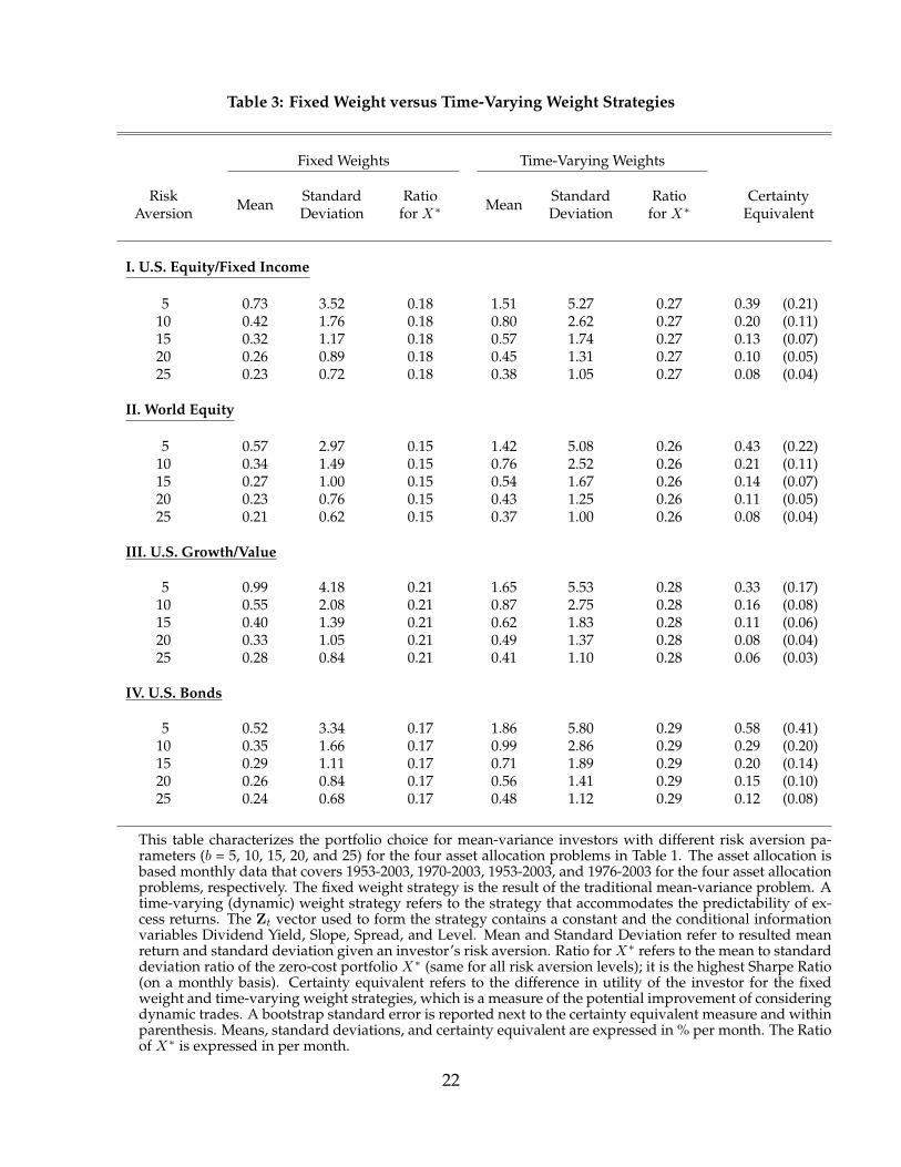
Table 3: Fixed Weight versus Time-Varying Weight Strategies

Fixed Weights Time-Varying Weights

RiskAversion Mean Standard

DeviationRatio

for X∗ Mean StandardDeviation

Ratiofor X∗

CertaintyEquivalent

I. U.S. Equity/Fixed Income

5 0.73 3.52 0.18 1.51 5.27 0.27 0.39 (0.21)10 0.42 1.76 0.18 0.80 2.62 0.27 0.20 (0.11)15 0.32 1.17 0.18 0.57 1.74 0.27 0.13 (0.07)20 0.26 0.89 0.18 0.45 1.31 0.27 0.10 (0.05)25 0.23 0.72 0.18 0.38 1.05 0.27 0.08 (0.04)

II. World Equity

5 0.57 2.97 0.15 1.42 5.08 0.26 0.43 (0.22)10 0.34 1.49 0.15 0.76 2.52 0.26 0.21 (0.11)15 0.27 1.00 0.15 0.54 1.67 0.26 0.14 (0.07)20 0.23 0.76 0.15 0.43 1.25 0.26 0.11 (0.05)25 0.21 0.62 0.15 0.37 1.00 0.26 0.08 (0.04)

III. U.S. Growth/Value

5 0.99 4.18 0.21 1.65 5.53 0.28 0.33 (0.17)10 0.55 2.08 0.21 0.87 2.75 0.28 0.16 (0.08)15 0.40 1.39 0.21 0.62 1.83 0.28 0.11 (0.06)20 0.33 1.05 0.21 0.49 1.37 0.28 0.08 (0.04)25 0.28 0.84 0.21 0.41 1.10 0.28 0.06 (0.03)

IV. U.S. Bonds

5 0.52 3.34 0.17 1.86 5.80 0.29 0.58 (0.41)10 0.35 1.66 0.17 0.99 2.86 0.29 0.29 (0.20)15 0.29 1.11 0.17 0.71 1.89 0.29 0.20 (0.14)20 0.26 0.84 0.17 0.56 1.41 0.29 0.15 (0.10)25 0.24 0.68 0.17 0.48 1.12 0.29 0.12 (0.08)

This table characterizes the portfolio choice for mean-variance investors with different risk aversion pa-rameters (b = 5, 10, 15, 20, and 25) for the four asset allocation problems in Table 1. The asset allocation isbased monthly data that covers 1953-2003, 1970-2003, 1953-2003, and 1976-2003 for the four asset allocationproblems, respectively. The fixed weight strategy is the result of the traditional mean-variance problem. Atime-varying (dynamic) weight strategy refers to the strategy that accommodates the predictability of ex-cess returns. The Zt vector used to form the strategy contains a constant and the conditional informationvariables Dividend Yield, Slope, Spread, and Level. Mean and Standard Deviation refer to resulted meanreturn and standard deviation given an investor’s risk aversion. Ratio for X∗ refers to the mean to standarddeviation ratio of the zero-cost portfolio X∗ (same for all risk aversion levels); it is the highest Sharpe Ratio(on a monthly basis). Certainty equivalent refers to the difference in utility of the investor for the fixedweight and time-varying weight strategies, which is a measure of the potential improvement of consideringdynamic trades. A bootstrap standard error is reported next to the certainty equivalent measure and withinparenthesis. Means, standard deviations, and certainty equivalent are expressed in % per month. The Ratioof X∗ is expressed in per month.

22

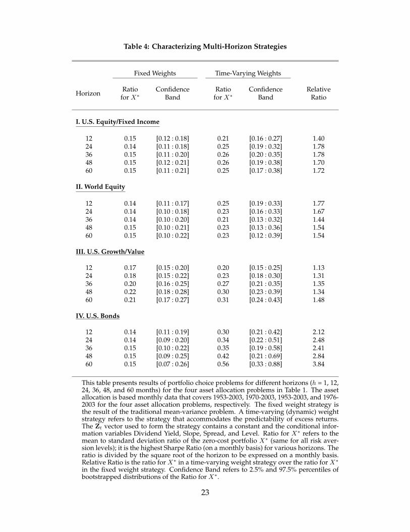
Table 4: Characterizing Multi-Horizon Strategies

Fixed Weights Time-Varying Weights

Horizon Ratiofor X∗

ConfidenceBand

Ratiofor X∗

ConfidenceBand

RelativeRatio

I. U.S. Equity/Fixed Income

12 0.15 [0.12 : 0.18] 0.21 [0.16 : 0.27] 1.4024 0.14 [0.11 : 0.18] 0.25 [0.19 : 0.32] 1.7836 0.15 [0.11 : 0.20] 0.26 [0.20 : 0.35] 1.7848 0.15 [0.12 : 0.21] 0.26 [0.19 : 0.38] 1.7060 0.15 [0.11 : 0.21] 0.25 [0.17 : 0.38] 1.72

II. World Equity

12 0.14 [0.11 : 0.17] 0.25 [0.19 : 0.33] 1.7724 0.14 [0.10 : 0.18] 0.23 [0.16 : 0.33] 1.6736 0.14 [0.10 : 0.20] 0.21 [0.13 : 0.32] 1.4448 0.15 [0.10 : 0.21] 0.23 [0.13 : 0.36] 1.5460 0.15 [0.10 : 0.22] 0.23 [0.12 : 0.39] 1.54

III. U.S. Growth/Value

12 0.17 [0.15 : 0.20] 0.20 [0.15 : 0.25] 1.1324 0.18 [0.15 : 0.22] 0.23 [0.18 : 0.30] 1.3136 0.20 [0.16 : 0.25] 0.27 [0.21 : 0.35] 1.3548 0.22 [0.18 : 0.28] 0.30 [0.23 : 0.39] 1.3460 0.21 [0.17 : 0.27] 0.31 [0.24 : 0.43] 1.48

IV. U.S. Bonds

12 0.14 [0.11 : 0.19] 0.30 [0.21 : 0.42] 2.1224 0.14 [0.09 : 0.20] 0.34 [0.22 : 0.51] 2.4836 0.15 [0.10 : 0.22] 0.35 [0.19 : 0.58] 2.4148 0.15 [0.09 : 0.25] 0.42 [0.21 : 0.69] 2.8460 0.15 [0.07 : 0.26] 0.56 [0.33 : 0.88] 3.84

This table presents results of portfolio choice problems for different horizons (h = 1, 12,24, 36, 48, and 60 months) for the four asset allocation problems in Table 1. The assetallocation is based monthly data that covers 1953-2003, 1970-2003, 1953-2003, and 1976-2003 for the four asset allocation problems, respectively. The fixed weight strategy isthe result of the traditional mean-variance problem. A time-varying (dynamic) weightstrategy refers to the strategy that accommodates the predictability of excess returns.The Zt vector used to form the strategy contains a constant and the conditional infor-mation variables Dividend Yield, Slope, Spread, and Level. Ratio for X∗ refers to themean to standard deviation ratio of the zero-cost portfolio X∗ (same for all risk aver-sion levels); it is the highest Sharpe Ratio (on a monthly basis) for various horizons. Theratio is divided by the square root of the horizon to be expressed on a monthly basis.Relative Ratio is the ratio for X∗ in a time-varying weight strategy over the ratio for X∗

in the fixed weight strategy. Confidence Band refers to 2.5% and 97.5% percentiles ofbootstrapped distributions of the Ratio for X∗.

23

Table 5: Certainty Equivalent: Time-Varying Weights versus Fixed Weights

Horizon

RiskAversion 12 24 36 48 60

I. U.S. Equity/Fixed Income

5 0.23 (0.13) 0.44 (0.15) 0.46 (0.17) 0.43 (0.21) 0.40 (0.25)10 0.12 (0.07) 0.22 (0.07) 0.23 (0.09) 0.21 (0.11) 0.19 (0.13)15 0.09 (0.04) 0.15 (0.05) 0.16 (0.06) 0.14 (0.07) 0.12 (0.09)20 0.07 (0.03) 0.12 (0.04) 0.12 (0.04) 0.10 (0.05) 0.08 (0.06)25 0.06 (0.03) 0.10 (0.03) 0.10 (0.04) 0.08 (0.04) 0.06 (0.05)

II. World Equity

5 0.41 (0.16) 0.31 (0.19) 0.18 (0.23) 0.27 (0.29) 0.28 (0.37)10 0.20 (0.08) 0.14 (0.09) 0.08 (0.11) 0.13 (0.14) 0.14 (0.19)15 0.14 (0.05) 0.08 (0.06) 0.05 (0.08) 0.09 (0.10) 0.09 (0.13)20 0.10 (0.04) 0.06 (0.05) 0.04 (0.06) 0.07 (0.07) 0.07 (0.10)25 0.08 (0.03) 0.04 (0.04) 0.03 (0.05) 0.06 (0.06) 0.06 (0.08)

III. U.S. Growth/Value

5 0.08 (0.09) 0.22 (0.10) 0.32 (0.12) 0.39 (0.15) 0.50 (0.18)10 0.04 (0.05) 0.11 (0.05) 0.16 (0.06) 0.20 (0.07) 0.25 (0.09)15 0.03 (0.03) 0.08 (0.03) 0.12 (0.04) 0.14 (0.05) 0.17 (0.06)20 0.02 (0.02) 0.06 (0.03) 0.09 (0.03) 0.11 (0.04) 0.14 (0.04)25 0.02 (0.02) 0.06 (0.02) 0.08 (0.02) 0.10 (0.03) 0.12 (0.04)

IV. U.S. Bonds

5 0.74 (0.36) 0.95 (0.57) 1.01 (0.89) 1.53 (1.20) 2.89 (1.67)10 0.38 (0.18) 0.47 (0.29) 0.50 (0.45) 0.77 (0.60) 1.45 (0.84)15 0.26 (0.12) 0.31 (0.19) 0.33 (0.30) 0.51 (0.40) 0.97 (0.56)20 0.20 (0.09) 0.23 (0.15) 0.25 (0.22) 0.39 (0.30) 0.73 (0.42)25 0.17 (0.07) 0.19 (0.12) 0.20 (0.18) 0.31 (0.24) 0.59 (0.34)

This table presents the certainty equivalent between a time-varying weight strategy and a fixedweight strategy for mean-variance investors with different risk aversion parameters (b = 5, 10, 15,20, and 25) and over different horizons (h = 12, 24, 36, 48, and 60 months) for the four asset allocationproblems in Table 1. The asset allocation is based monthly data that covers 1953-2003, 1970-2003,1953-2003, and 1976-2003 for the four asset allocation problems, respectively. The certainty equiva-lent is multiplied by 100 and divided by the horizon to be expressed in % and on a monthly basis. Abootstrap standard error is reported next to the certainty equivalent measure and within parenthe-sis. The fixed weight strategy is the result of the traditional mean-variance problem. A time-varying(dynamic) weight strategy refers to the strategy that accommodates the predictability of excess re-turns. The Zt vector used to form the strategy contains a constant and the conditional informationvariables Dividend Yield, Slope, Spread, and Level.

24

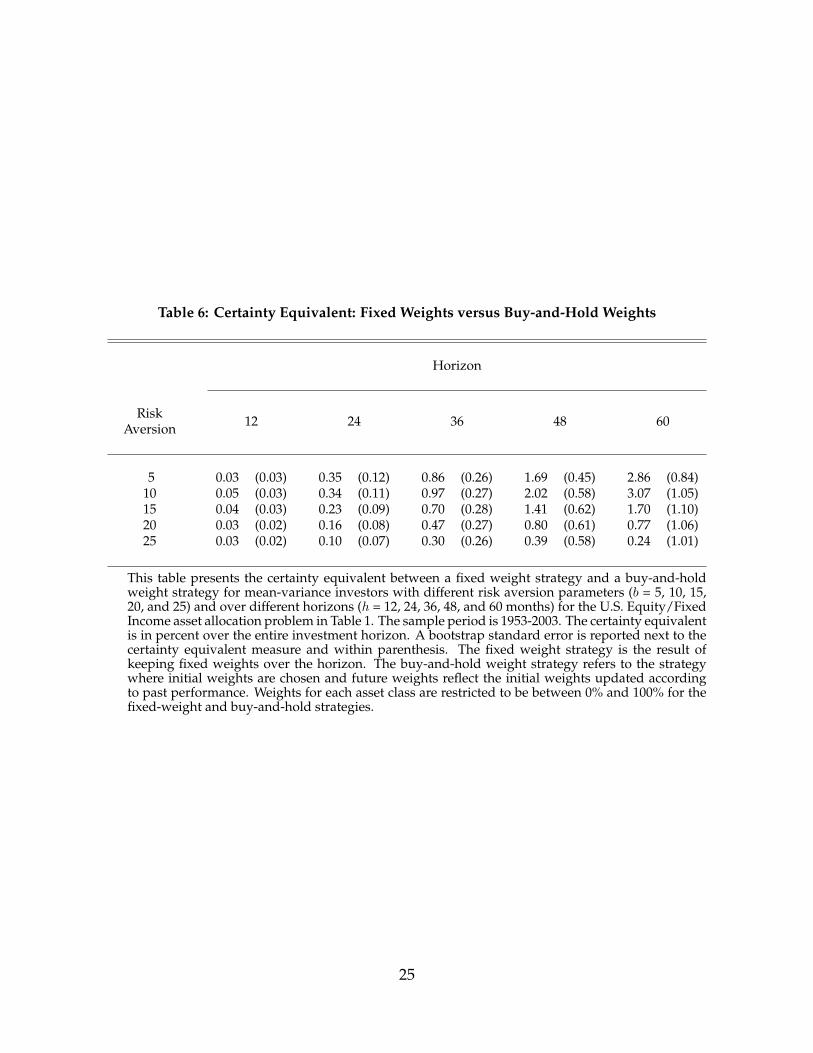
Table 6: Certainty Equivalent: Fixed Weights versus Buy-and-Hold Weights

Horizon

RiskAversion 12 24 36 48 60

5 0.03 (0.03) 0.35 (0.12) 0.86 (0.26) 1.69 (0.45) 2.86 (0.84)10 0.05 (0.03) 0.34 (0.11) 0.97 (0.27) 2.02 (0.58) 3.07 (1.05)15 0.04 (0.03) 0.23 (0.09) 0.70 (0.28) 1.41 (0.62) 1.70 (1.10)20 0.03 (0.02) 0.16 (0.08) 0.47 (0.27) 0.80 (0.61) 0.77 (1.06)25 0.03 (0.02) 0.10 (0.07) 0.30 (0.26) 0.39 (0.58) 0.24 (1.01)

This table presents the certainty equivalent between a fixed weight strategy and a buy-and-holdweight strategy for mean-variance investors with different risk aversion parameters (b = 5, 10, 15,20, and 25) and over different horizons (h = 12, 24, 36, 48, and 60 months) for the U.S. Equity/FixedIncome asset allocation problem in Table 1. The sample period is 1953-2003. The certainty equivalentis in percent over the entire investment horizon. A bootstrap standard error is reported next to thecertainty equivalent measure and within parenthesis. The fixed weight strategy is the result ofkeeping fixed weights over the horizon. The buy-and-hold weight strategy refers to the strategywhere initial weights are chosen and future weights reflect the initial weights updated accordingto past performance. Weights for each asset class are restricted to be between 0% and 100% for thefixed-weight and buy-and-hold strategies.

25

Figu

re1:

Mea

n–

Stan

dard

Dev

iati

onFr

onti

ers:

Fixe

dan

dTi

me-

Var

ying

Wei

ghts

The

figur

esh

ows

95%

confi

denc

eba

nds

for

unco

ndit

iona

lmea

n–

stan

dard

devi

atio

nfr

onti

ers

for

fixed

wei

ght(

solid

curv

e)an

dti

me-

vary

ing

wei

ght

(das

hed

curv

e)st

rate

gies

fort

hefo

uras

seta

lloca

tion

prob

lem

sin

Tabl

e1.

The

asse

tallo

cati

onis

base

dm

onth

lyda

tath

atco

vers

1953

-200

3,19

70-2

003,

1953

-200

3,an

d19

76-2

003

for

the

four

asse

tal

loca

tion

prob

lem

s,re

spec

tive

ly.

The

curv

esre

pres

ent

the

low

er(2

.5%

)an

dup

per

(97.

5%)

fron

tier

sfo

rth

est

rate

gies

.Th

eZ

tve

ctor

used

tofo

rmth

eti

me-

vary

ing

wei

ghts

trat

egy

cont

ains

aco

nsta

ntan

dth

eco

ndit

iona

linf

orm

atio

nva

riab

les

Div

iden

dYi

eld,

Slop

e,Sp

read

,and

Leve

l.Th

efil

led

squa

res

show

the

aver

ages

and

stan

dard

devi

atio

nsof

the

real

retu

rns

ofth

eba

seas

sets

inea

chas

set

allo

cati

onpr

oble

m.

26