NBER WORKING PAPER SERIES

PRICE RIGIDITIES AND THE GRANULAR ORIGINS OF AGGREGATE FLUCTUATIONS

Ernesto PastenRaphael Schoenle

Michael Weber

Working Paper 23750http://www.nber.org/papers/w23750

NATIONAL BUREAU OF ECONOMIC RESEARCH1050 Massachusetts Avenue

Cambridge, MA 02138August 2017

We thank Susanto Basu, Ben Bernanke, Francesco Bianchi, Saki Bigio, Carlos Carvalho, Stephen Cecchetti, John Cochrane, Eduardo Engel, Xavier Gabaix, Yuriy Gorodnichenko, Gita Gopinath, Basile Grassi, Josh Hausman, Pete Klenow, Jennifer La’O, Glenn Magerman, Valerie Ramey, Alireza Tahbaz-Salehi, Harald Uhlig, and conference and seminar participants at the Boston Fed, Central Bank of Chile, ESSIM, the 2017 LSE Workshop on Networks in Macro and Finance, the NBER Monetary Economics 2017 Spring Meeting, Maryland, PUC-Chile, UCLA, Stanford, UChile-Econ, UVA as well as the 2016 SED Meeting (Toulouse). Pasten thanks the support of the Universite de Toulouse Capitole during his stays in Toulouse. The contributions by Michael Weber to this paper have been prepared under the 2016 Lamfalussy Fellowship Program sponsored by the European Central Bank. Any views expressed are only those of the authors and do not necessarily represent the views of the ECB or the Eurosystem or the Central Bank of Chile. We also thank Jose Miguel Alvarado, Will Cassidy, Stephen Lamb, and Matt Klepacz for excellent research assistance. The views expressed herein are those of the authors and do not necessarily reflect the views of the National Bureau of Economic Research.

NBER working papers are circulated for discussion and comment purposes. They have not been peer-reviewed or been subject to the review by the NBER Board of Directors that accompanies official NBER publications.

© 2017 by Ernesto Pasten, Raphael Schoenle, and Michael Weber. All rights reserved. Short sections of text, not to exceed two paragraphs, may be quoted without explicit permission provided that full credit, including © notice, is given to the source.

Price Rigidities and the Granular Origins of Aggregate FluctuationsErnesto Pasten, Raphael Schoenle, and Michael WeberNBER Working Paper No. 23750August 2017JEL No. E31,E32,O40

ABSTRACT

We study the aggregate implications of sectoral shocks in a multi-sector New Keynesian model featuring sectoral heterogeneity in price stickiness, sector size, and input-output linkages. We calibrate a 341 sector version of the model to the United States. Both theoretically and empirically, sectoral heterogeneity in price rigidity (i) generates sizable GDP volatility from sectoral shocks, (ii) amplifies both the "granular" and the "network" effects, (iii) alters the identity and relative contributions of the most important sectors for aggregate fluctuations, (iv) can change the sign of fluctuations, (v) invalidates the Hulten Theorem, and (vi) generates a frictional origin of aggregate fluctuations.

Ernesto PastenCentral Bank of ChileAgustinas 1180SantiagoChileand Toulouse School of Economics ernesto.pasten@tse-fr.eu

Raphael SchoenleBrandeis UniversityDepartment of EconomicsMail Stop 021415 South StreetWaltham, MA 02454schoenle@brandeis.edu

Michael WeberBooth School of BusinessUniversity of Chicago5807 South Woodlawn AvenueChicago, IL 60637and NBERmichael.weber@chicagobooth.edu

I Introduction

Identifying aggregate shocks that drive business cycles might be difficult (Cochrane (1994)). A

recent literature advances the possibility that shocks at the firm or sector level may be the origin

of aggregate fluctuations. This view stands in contrast to the “diversification argument” of Lucas

(1977), which conjectures idiosyncratic shocks at a highly disaggregated level average out.1 In

contrast, Gabaix (2011) argues the diversification argument does not readily apply when the

firm-size distribution is fat-tailed, which is the empirically relevant case for the United States.

Intuitively, shocks to disproportionately large firms matter for aggregate fluctuations, known

as the “granular” effect. In a similar vein, Acemoglu, Carvalho, Ozdaglar, and Tahbaz-Salehi

(2012) focus on sectoral shocks and show that input-output relationships across sectors can mute

the diversification argument if measures of sector centrality follow a fat-tailed distribution. They

label this channel the “network” channel. Thus, either through a granular or network channel,

microeconomic shocks to small numbers of firms or sectors may drive aggregate fluctuations.2

Prices are the key transmission mechanism of sectoral technology shocks to the economy.

But this prior work assumes prices are flexible which might not be an innocuous assumption. A

large literature documents prices might be sticky in the short run and prices for different goods

change at different frequencies. In fact, nominal price rigidities are a leading explanation for

the real effects of nominal shocks. For these reasons, we study whether and how price rigidity

affects the aggregate importance of microeconomic shocks.

To fix ideas, consider a multi-sector economy without linkages across sectors and consider

a positive productivity shock to one sector. Marginal costs in this sector decrease and prices

will fall in the absence of pricing frictions. But consider what happens if prices do not adjust.

Demand for goods remains unchanged, so production remains unchanged. Therefore, regardless

of the size of the sector, the contribution of its shocks to aggregate fluctuations is zero (except

for some general equilibrium effects).3 A similar logic applies to production networks. Following

a positive productivity shock, a price cut in one sector will propagate downstream by decreasing

production costs. This, in turn, will trigger price cuts in other sectors. But, if prices do not

change in the shocked sector, marginal costs of downstream firms remain unchanged and there

1Dupor (1999) takes a perspective similar to Lucas (1977) and implicitly so does anyone who models aggregateshocks driving aggregate fluctuations.

2A fast-growing literature has followed. Some recent examples are Acemoglu, Akcigit, and Kerr (2016);Acemoglu, Ozdaglar, and Tahbaz-Salehi (2017); Atalay (2015); Baqaee (2016); Bigio and La’O (2016); Caliendo,Parro, Rossi-Hansberg, and Sarte (2014); Carvalho and Gabaix (2013); Carvalho and Grassi (2015); Di Giovanni,Levchenko, and Mejean (2014); Di Giovanni, Levchenko, and Mejean (2016); Foerster, Sarte, and Watson (2011);Ozdagli and Weber (2016); Grassi (2017); and Baqaee and Farhi (2017).

3First, lower demand for inputs in the shocked sector decreases wages. Second, higher profits of firms in theshocked sector increase household income. However, these effects are small up to a first-order approximation.

2

is no propagation regardless of the centrality of the shocked sector.

In the data, prices are neither fully rigid nor fully flexible, and substantial heterogeneity of

price rigidity exists across sectors in the United States (see Bils and Klenow (2004); Klenow and

Kryvtsov (2008); Nakamura and Steinsson (2008)). How does the heterogeneity in nominal

price rigidity interact with the granular effect of Gabaix (2011) and the network effect of

Acemoglu et al. (2012) in affecting the power of microeconomic shocks to generate sizable

aggregate fluctuations? Do price rigidities distort the identity of sectors that are the origin of

aggregate fluctuations? Can price rigidity create a “frictional” origin of aggregate fluctuations,

conceptually different from the granular or the network origins the literature already describes?

We study these questions in a multi-sector New Keynesian model in which firms produce

output using labor and intermediate inputs. Our answers are yes and yes: heterogeneity in

price rigidities changes the identity of sectors from which aggregate fluctuations originate, and

generates GDP volatility from sectoral shocks independent of the sector-size distribution and

network centrality. Our model follows Basu (1995) and Carvalho and Lee (2011), but we make no

simplifying assumptions on the steady-state distribution of sectoral size, input-output linkages,

and the sectoral distribution of price-setting frictions that we model following Calvo (1983).4

Sectoral productivity shocks are the only source of variation in our model.

As a first step, we analytically study in a simplified version of our model the distortionary

role of price rigidity on the granular and network origins of aggregate fluctuations. Up to a

log-linear approximation, GDP is a linear combination of sectoral shocks, and the model nests

Gabaix (2011) and Acemoglu et al. (2012) as special cases. When we abstract from intermediate

inputs and price stickiness, we recover the granularity effect of Gabaix (2011): the ability of

microeconomic shocks to generate aggregate fluctuations depends on the fat-tailedness of the

sector-size distribution, which we measure by sector GDP.

But price stickiness introduces three new effects. First, it dampens the level of aggregate

volatility originating from any shock, both sector-specific and aggregate. This is a conventional

effect in New Keynesian models. Second, a novel relative effect arises: the sectoral distribution of

price rigidity distorts the relative importance of sectors for aggregate fluctuations. In particular,

a sector is important when it is large, as in Gabaix (2011), and/ or when its prices are much more

flexible than most prices in the economy. Consider a scenario in which the sector-size distribution

is fat-tailed and size is negatively correlated with price rigidity; that is, larger sectors are more

likely to have more flexible prices. In this case, shocks to large sectors become even more

4We argue below that our results are most likely stronger in models with state-dependent pricing. Anyprice-adjustment technology should deliver our key results, as long as price rigidity is heterogeneous. We chooseCalvo pricing as an expository tool, and for computational reasons.

3

important for aggregate volatility than in a frictionless economy, because large sectors are now

effectively larger. They pass through relatively more of a shock. In other words, the distribution

of the multipliers mapping sectoral shocks into aggregate fluctuations is more fat-tailed than

implied by the pure sector-size distribution alone. The opposite holds if sector size is positively

correlated with price rigidity. The diversification argument of Lucas (1977) might even gain

bite due to sticky prices, although the conditions necessary for the granular channel hold in a

frictionless economy. In short, whenever the ranking of flexible sectors in a sticky-price economy

is sufficiently different from the ranking of the most important sectors in an economy with

flexible prices, price rigidity will distort the effect of sectoral shocks on aggregate fluctuations.

Third, because heterogeneous price rigidity re-weights the importance of sectors for aggregate

fluctuations, it may even distort the sign the business cycles and not only generate inertia, as is

standard with aggregate shocks.

We reach similar results for the network effect of Acemoglu et al. (2012). We know from

Acemoglu et al. (2012), with flexible prices, microeconomic shocks are more important for

macroeconomic volatility if the distribution of sector centrality is more fat-tailed: large suppliers

of intermediate inputs (first-order interconnection) and/ or large suppliers to large suppliers of

intermediate inputs (second-order interconnection) are important for aggregate volatility. With

price stickiness, the most flexible sectors among large suppliers of intermediate inputs and/

or the most flexible sectors among large suppliers to the most flexible large intermediate input

suppliers are now the most important determinants of aggregate volatility. Thus, the multipliers

of sectoral shocks to aggregate volatility may be more or less fat-tailed than the distribution of

sector centrality. Heterogeneity in price rigidity invalidates the Hulten (1978) result that holds

in Gabaix (2011) and Acemoglu et al. (2012): sector (or firm) total sales is no longer a sufficient

statistic for the importance of GDP volatility.

In a second step, we show the quantitative importance of sectoral shocks to drive aggregate

fluctuations. We calibrate the model to the input-output tables of the Bureau of Economic

Analysis (BEA) at the most disaggregated level and the micro data underlying the Producer

Price Index (PPI) from the Bureau of Labor Statistics (BLS). After merging these two datasets,

we end up with 341 sectors. We conduct a series of experiments within our 341-sector

economy. Price rigidity does indeed substantially affect the importance of microeconomic

shocks for aggregate fluctuations. We base the following discussion on relative multipliers,

that is, multipliers of sectoral productivity shocks on GDP volatility relative to the multiplier of

aggregate productivity shocks on GDP volatility, because the effect of aggregate shocks is not

invariant to the distribution of price rigidity, sectoral GDP, and input-output linkages.

4

In our first experiment, we match sectoral GDP shares but assume equal input-output

linkages across sectors. The relative multiplier of sectoral productivity shocks on GDP volatility

increases from 11% when prices are flexible to 33.7% when price stickiness across sectors follows

the empirical distribution. In the second experiment, we match input-output linkages to the U.S.

data but assume equal sector sizes. Now, the relative multiplier increases from 8% with flexible

prices to 13.2%. In a third experiment, differences in the frequency of price changes are the only

source of heterogeneity across sectors. The relative multiplier of sectoral shocks is now 12.4%,

more than twice as large compared to the multiplier in an economy with complete symmetry

and equal price stickiness across sectors. This result suggests a “frictional” origin of aggregate

fluctuations: heterogeneity in price stickiness alone can generate aggregate fluctuations from

sectoral shocks.

Overall, when all three heterogeneities are present, the relative multiplier on GDP volatility

is 32%, almost six times larger than in an economy with complete symmetry across sectors. The

six-fold increase of the relative multiplier underscores the relevance of microeconomic shocks

for aggregate fluctuations, and shows heterogeneities in sector size, input-output structure, and

price stickiness are intricately linked and reinforce each other.

But price rigidity does not only contribute to the importance of micro shocks driving

aggregate volatility. Differences in price rigidity across sectors have also strong effects on the

identity and contribution of sectors driving aggregate fluctuations. For instance, the identity

of the two most important sectors for aggregate volatility shifts from “Real Estate,” and

“Wholesale Trading” with flexible prices to “Oil and Gas Extraction” and “Dairy cattle and milk

production” with heterogeneous sticky prices when we only consider network effects. When we

also allow for sectoral heterogeneity in sector size, the two most important sectors with flexible

prices are “Retail trade” and “Real Estate” but “Monetary authorities and depository credit

intermediation” and “Wholesale Trading” with sticky prices.

At an abstract level, our analysis does not only show that the size or centrality of nodes

in the network matters for the macro effect of micro shocks, but also the frictions that affect

the capacity of nodes to propagate shocks. This point goes beyond sticky prices. Nonetheless,

we focus on sticky prices for two reasons. First, prices are the central transmission mechanism

of sectoral shocks in production networks. Of course, nodes may be differentially important for

GDP fluctuations due to other frictions, such as financial frictions. But pricing frictions are first

order because they determine the propagation mechanism through the production networks.

They simultaneously affect the transmission of shocks on top of all other frictions by directly

influencing demand and supply. Second, price stickiness is a measurable friction at a highly

5

disaggregated level.

The frictional origin of fluctuations also goes beyond production networks in a closed

economy; it applies to all networks with heterogeneous effects of frictions across nodes, for

example, in international trade networks, financial networks, or social networks. Our work is

thus related to an extensive literature that we do not attempt to summarize here; instead, we

only highlight the papers that are most closely related below.

A. Literature review

Long and Plosser (1983) pioneer the microeconomic origin of aggregate fluctuations, and Horvath

(1998) and Horvath (2000) push this literature forward. Dupor (1999) argues microeconomic

shocks matter only due to poor disaggregation. Gabaix (2011) invokes the firm size-distribution,

and Acemoglu et al. (2012) assert the sectoral network structure of the economy to document

convincingly the importance of microeconomic shocks for macroeconomic fluctuations: under

empirically plausible assumptions, microeconomic shocks do matter. Barrot and Sauvagnat

(2016), Acemoglu et al. (2016), and Carvalho, Nirei, Saito, and Tahbaz-Salehi (2016) provide

empirical evidence for the importance of idiosyncratic shocks for aggregate fluctuations, and

Carvalho (2014) synthesizes this literature.

The distortionary role of frictions (and price rigidity in particular) is at the core of

the business-cycle literature that conceptualizes aggregate shocks as the driver of aggregate

fluctuations, including the New Keynesian literature. However, to the best of our knowledge,

no parallel study of the distortionary role of frictions exists when aggregate fluctuations have

microeconomic origins. That said, a few recent papers include frictions in their analyses. Baqaee

(2016) shows entry and exit of firms coupled with CES preferences may amplify the aggregate

effect of microeconomic shocks. Carvalho and Grassi (2015) study the effect of large firms

in a quantitative business-cycle model with entry and exit. Bigio and La’O (2016) study the

aggregate effects of the tightening of financial frictions in a production network. Despite a

different focus, we share our finding with Baqaee (2016) and Bigio and La’O (2016) that the

Hulten theorem does not apply in economies with frictions.

Our model shares building blocks with previous work studying pricing frictions in production

networks. Basu (1995) shows frictions introduce misallocation resulting in nominal demand

shocks looking like aggregate productivity shocks. Carvalho and Lee (2011) develop a New

Keynesian model in which firms’ prices respond slowly to aggregate shocks and quickly to

idiosyncratic shocks, rationalizing the findings in Boivin et al. (2009). We build on their

work to answer different questions and relax assumptions regarding the production structure

6

to quantitatively study the interactions of different heterogeneities.

Nakamura and Steinsson (2010), Midrigan (2011), and Alvarez, Le Bihan, and Lippi

(2016), among many others, endogenize price rigidity to study monetary non-neutrality in

multi-sector menu-cost models. Computational burden and calibration issues make such an

approach infeasible in our highly disaggregated model which is why we study the effect of

disaggregation on monetary non-neutrality in a multi-sector Calvo model in a companion paper

(Pasten, Schoenle, and Weber (2016)). Bouakez, Cardia, and Ruge-Murcia (2014) estimate

a Calvo model with production networks, using data for 30 sectors, and find heterogeneous

responses of sectoral inflation to a monetary policy shock, but do not study the questions we

pose in this paper.

Other recent applications of networks in different areas of macroeconomics and finance

are Gofman (2011), who studies how intermediation in over-the-counter markets affects the

efficiency of resource allocation, Di Maggio and Tahbaz-Salehi (2015), who study the fragility

of the interbank market, Ozdagli and Weber (2016), who show empirically that input-output

linkages are a key propagation channel of monetary policy shocks to the stock market, and

Kelly, Lustig, and Van Nieuwerburgh (2013), who study the joined dynamics of the firm-size

distribution and stock return volatilities. Herskovic, Kelly, Lustig, and Van Nieuwerburgh (2016)

and Herskovic (2015) study the asset-pricing implications of production networks.

II Model

Our multi-sector model has households supplying labor and demanding goods for final

consumption, firms with sticky prices producing varieties of goods with labor and intermediate

inputs, and a monetary authority setting nominal interest rates according to a Taylor rule.

Sectors are heterogeneous in three dimensions: their final goods production, input-output

linkages, and the frequency of price adjustment.

A. Households

The representative household solves

maxCt,Lkt∞t=0

E0

∞∑t=0

βt

(C1−σt − 1

1− σ−

K∑k=1

gkL1+ϕkt

1 + ϕ

),

7

subject to

K∑k=1

WktLkt +K∑k=1

Πkt + It−1Bt−1 −Bt = P ct Ct

K∑k=1

Lkt ≤ 1,

where Ct and P ct are aggregate consumption and aggregate prices, respectively. Lkt and Wkt are

labor employed and wages are paid in sector k = 1, ...,K. Households own firms and receive net

income, Πkt, as dividends. Bonds, Bt−1, pay a nominal gross interest rate of It−1. Total labor

supply is normalized to 1.

Households’ demand of final goods, Ct, and goods produced in sector k, Ckt, are

Ct ≡

[K∑k=1

ω1η

ckC1− 1

η

kt

] ηη−1

, (1)

Ckt ≡[n−1/θk

∫=kC

1− 1θ

jkt dj

] θθ−1

. (2)

A continuum of goods indexed by j ∈ [0, 1] exists with total measure 1. Each good belongs to one

of the K sectors in the economy. Mathematically, the set of goods is partitioned into K subsets

=kKk=1 with associated measures nkKk=1 such that∑K

k=1 nk = 1.5 We allow the elasticity of

substitution across sectors η to differ from the elasticity of substitution within sectors θ.

The first key ingredient of our model is the vector of weights Ωc ≡ [ωc1, ..., ωcK ] in equation

(1). These weights show up in households’ sectoral demand:

Ckt = ωck

(PktP ct

)−ηCt. (3)

All prices are identical in steady state, so ωck ≡ CkC , where variables without a time subscript are

steady-state quantities. In our economy, Ct represent the total production of final goods, that

is, GDP. The vector Ωc represents steady-state sectoral GDP shares satisfying Ω′cι = 1 where ι

denotes a column-vector of 1s. Away from the steady state, sectoral GDP shares depend on the

gap between sectoral prices and the aggregate price index, P ct :

P ct =

[K∑k=1

ωckP1−ηkt

] 11−η

. (4)

5The sectoral subindex is redundant, but it clarifies exposition. Note we can interpret nk as the sectoral sharein gross output.

8

We can interpret P ct as GDP deflator. Households’ demand for goods within a sector is given

by

Cjkt =1

nk

(PjktPkt

)−θCkt for k = 1, ...,K. (5)

Goods within a sector share sectoral consumption equally in steady state. Away from the steady

state, the demand of goods within a sector is distorted by the gap between a firm’s price and

the sectoral price, defined as

Pkt =

[1

nk

∫=kP 1−θjkt dj

] 11−θ

for k = 1, ...,K. (6)

The household first-order conditions determine labor supply and the Euler equation:

Wkt

P ct= gkL

ϕktC

σt for all k, j, (7)

1 = Et

[β

(Ct+1

Ct

)−σItP ctP ct+1

]. (8)

We implicitly assume sectoral segmentation of labor markets, so labor supply in equation (7)

holds for a sector-specific wage WktKk=1. We choose the parameters gkKk=1 to ensure a

symmetric steady state across all firms.

B. Firms

A continuum of monopolistically competitive firms exists in the economy operating in different

sectors. We index firms by their sector, k = 1, ...K, and by j ∈ [0, 1]. The production function

is

Yjkt = eaktL1−δjkt Z

δjkt, (9)

where akt is an i.i.d. productivity shock to sector k with E [akt] = 0 and V [akt] = v2 for all k,

Ljkt is labor, and Zjkt is an aggregator of intermediate inputs:

Zjkt ≡

[K∑k′=1

ω1η

kk′Zjk(k′)1− 1

η

] ηη−1

. (10)

Zkjt (r) is the amount of goods firm j in sector k uses in period t as intermediate inputs from

sector r.

The second key ingredient of our model is heterogeneity in aggregator weights ωkk′k,k′ .

We denote these weights in matrix notation as Ω, satisfying Ωι = ι. The demand of firm jk for

9

goods produced in sector k′ is given by

Zjkt(k′)

= ωkk′

(Pk′t

P kt

)−ηZjkt. (11)

We can interpret ωkk′ as the steady-state share of goods from sector k′ in the intermediate input

use of sector k, which determines the input-output linkages across sectors in steady state. Away

from the steady state, the gap between the price of goods in sector k′ and the aggregate price

relevant for a firm in sector k, P kt distorts input-output linkages:

P kt =

[K∑k′=1

ωkk′P1−ηk′t

] 11−η

for k = 1, ...,K. (12)

P kt uses the sector-specific steady-state input-output linkages to aggregate sectoral prices.

The aggregator Zjk (k′) gives the demand of firm jk for goods in sector k′:

Zjk(k′)≡

[n−1/θk′

∫=k′

Zjkt(j′, k′

)1− 1θ dj′

] θθ−1

. (13)

Firm jk’s demand for an arbitrary good j′ from sector k′ is

Zjkt(j′, k′

)=

1

nk′

(Pj′′k′tPk′t

)−θZjk

(k′). (14)

In steady state, all firms within a sector share the intermediate input demand of other

sectors equally. Away from the steady state, the gap between a firm’s price and the price

index of the sector it belongs to (see equation (6)) distorts the firm’s share in the production of

intermediate input. Our economy has K + 1 different aggregate prices, one for the household

sector and one for each of the K sectors. By contrast, the household sector and all sectors face

unique sectoral prices.

The third key ingredient of our model is sectoral heterogeneity in price rigidity. Specifically,

we model price rigidity a la Calvo6 with parameters αkKk=1 such that the pricing problem of

firm jk is

maxPjkt

Et∞∑s=0

Qt,t+sατk [PjktYjkt+s −MCkt+sYjkt+s] .

6The computational burden with several hundred sector-specific state variables imposes prohibitive limitationson most endogenous price adjustment technologies, such as menu costs. However, as will become clear, our mainpoint about the importance of heterogeneous-price stickiness is, to a first order, due to the relative differenceacross firms, a modeling feature that endogenous price adjustment technologies will preserve.

10

Marginal costs are MCkt = 11−δ

(δ

1−δ

)−δe−aktW 1−δ

kt

(P kt)δ

in reduced form after imposing the

optimal mix of labor and intermediate inputs:

δWktLjkt = (1− δ)P kt Zjkt, (15)

and Qt,t+s is the stochastic discount factor between period t and t+ s.

We assume the elasticities of substitution across and within sectors are the same for

households and all firms. This assumption shuts down price discrimination among different

customers, and firms choose a single price P ∗kt:

∞∑τ=0

Qt,t+ταskYjkt+τ

[P ∗kt −

θ

θ − 1MCkt+τ

]= 0, (16)

where Yjkt+τ is the total production of firm jk in period t+ τ .

We define idiosyncratic shocks aktKk=1 at the sectoral level, and it follows that the optimal

price, P ∗kt, is the same for all firms in a given sector. Thus, aggregating among all prices within

sector yields

Pkt =[(1− αk)P ∗1−θkt + αkP

1−θkt−1

] 11−θ

for k = 1, ...,K. (17)

C. Monetary policy, equilibrium conditions, and definitions

The monetary authority sets nominal interest rates according to a Taylor rule:

It =1

β

(P ctP ct−1

)φπ (CtC

)φy. (18)

Monetary policy reacts to inflation, P ct /Pct−1, and deviations from steady state total value-added,

Ct/C. We do not model monetary policy shocks.

Bonds are in zero net supply, Bt = 0, labor markets clear, and goods markets clear such

that

Yjkt = Cjkt +

K∑k′=1

∫=k′

Zj′k′t (j, k) dj′, (19)

implying a wedge between gross output Yt and GDP Ct.

III Theoretical Results in a Simplified Model

We can derive closed-form results for the importance of sectoral shocks for aggregate fluctuations

in a simplified version of our model. Given the focus of the paper, we study log-linear deviations

11

from steady state. We report the steady-state solution and the full log-linear system solving for

the equilibrium in the Online Appendix. All variables in lower cases denote log-linear deviations

from steady state.

A. Simplifying Assumptions

We make the following simplifying assumptions:

(i) Households have log utility, σ = 1, and linear disutility of labor, ϕ = 0. Thus,

wkt = pct + ct;

that is, the labor market is integrated and nominal wages are proportional to nominal GDP.

(ii) Monetary policy targets constant nominal GDP, so

pct + ct = 0.

(iii) We replace Calvo price stickiness by a simple rule: all prices are flexible, but with

probability λk, a firm in sector k has to set its price before observing shocks. Thus,

Pjkt =

Et−1

[P ∗jkt

]with probability λk,

P ∗jkt with probability 1− λk,

where Et−1 is the expectation operator conditional on the t− 1 information set.

Solution We show in the Online Appendix that under assumptions (i), (ii), and (iii), ct

is given by

ct = χ′at, (20)

where χ ≡ (I− Λ) [I− δΩ′ (I− Λ)]−1 Ωc. Λ is a diagonal matrix with price-rigidity probabilities

[λ1, ..., λK ] as entries, and at ≡ [a1t, ..., aKt]′ is a vector of sectoral productivity shocks. Recall

Ωc and Ω represent in steady state the sectoral GDP shares and intermediate-input shares.

A linear combination of sectoral shocks describes the log-deviation of GDP from its steady

state up to a first-order approximation. Thus, aggregate GDP volatility is

vc = v

√√√√ K∑k=1

χ2k = ‖χ‖2 v, (21)

because all sectoral shocks have the same volatility; that is, V [akt] = v2 for all k. ‖χ‖2 denotes

12

the Euclidean norm of χ.

Thus, χ is a vector of multipliers from the volatility of sectoral productivity shocks to GDP

volatility. We will refer to these multipliers as sectoral multipliers in the following.

Below, we study the effect of heterogeneous price rigidity on the scale of aggregate volatility

vc in an economy with a given number of sectors K. We also investigate the effect on the rate

of decay of vc as the economy becomes increasingly more disaggregated, K →∞.

We use the following definition:

Definition 1 A given random variable X follows a power-law distribution with shape

parameter β when Pr (X > x) = (x/x0)−β for x ≥ x0 and β > 0.

B. The Granular Effect and Price Rigidity

We now study the interaction of price rigidity with the granular effect of Gabaix (2011). The

granular effect studies the role of the firm-size distribution on the importance of microeconomic

shocks as the origin of aggregate volatility. Gabaix (2011) measures firm size by total sales,

which includes sales as final goods and as intermediate inputs. By contrast, the setup of our

model and data requirements have us study sectors instead of firms. However, this difference is

only nominal.

We shut down intermediate inputs, that is, δ = 0, to disentangle the contribution of sales

as final goods from sales as intermediate inputs. Hence, sector size only depends on sectoral

consumption. With δ = 0, our expressions mirror the ones in Gabaix (2011) in special cases.

We study the effect of intermediate inputs, that is, the network effect of Acemoglu et al. (2012)

below.

When δ = 0,

χ =(I− Λ′

)Ωc,

or, simply, χk = (1− λk)ωck for all k.

Recall ωck = Ck/∑K

k=1Ck. Hence, steady-state sectoral GDP shares fully determine sectoral

multipliers only when prices are flexible. In general, sectoral multipliers also depend on

the sectoral distribution of price stickiness. Sales are no longer a sufficient statistic for the

importance of sectors for aggregate volatility breaking the Hulten (1978) result in the Gabaix

(2011) framework.

The following lemma presents our first result for homogeneous price stickiness across sectors.

13

Lemma 1 When δ = 0 and λk = λ for all k, then

vc =(1− λ) v

CkK1/2

√V (Ck) + C

2k,

where Ck and V (·) are the sample mean and sample variance of CkKk=1.7

This lemma follows from equation (21) when δ = 0. As in Gabaix (2011), the volatility of

GDP in an economy with K sectors depends on the cross-sectional dispersion of sector size, here

measured by V (Ck). Price rigidity only has a scale effect on volatility depending on whether

productivity shocks are sectoral or aggregate. The scale effect follows from equation (20): if

δ = 0, and all sectoral shocks are perfectly correlated, then vc = (1− λ) v. Active monetary

policy can correct this scale effect.

The next proposition determines the rate of decay of vc as the economy becomes increasingly

more disaggregated, K →∞, in the presence of homogeneous price stickiness.

Proposition 1 (Granular effect) If δ = 0, λk = λ for all k, and CkKk=1 follows a power-law

distribution with shape parameter βc ≥ 1, then

vc ∼

u0Kmin1−1/βc,1/2 v for βc > 1

u0logK for βc = 1

where u0 is a random variable independent of K and v.

Proof. See Online Appendix.

Proposition 1 revisits the central idea of the granular effect: when the size distribution of

sectors is fat-tailed, given by βc < 2, aggregate volatility vc converges to zero at a rate slower

than the Central Limit Theorem implies, which is K1/2. The rate of decay of vc becomes slower

as βc → 1. Intuitively, when the size distribution of sectors is fat-tailed, few sectors remain

disproportionately large at any level of disaggregation. Gabaix (2011) documents that a power-

law distribution with shape parameter close to 1 characterizes the upper tail of the empirical

distribution of firm sizes.8 Thus, contrary to Dupor (1999), sectoral shocks can generate sizable

aggregate fluctuations even if we study sectors at a highly disaggregated level. Homogeneous

price rigidity plays no role for this result, except for the scale effect we discuss in Lemma 1.

We now study the case of heterogeneous price rigidity across sectors.

7We define V (Xk) of a sequence XkKk=1 as V (Xk) ≡ 1K

∑Kk=1

(Xk −X

)2. The definition of the sample mean

is standard.8We find similar results with sectoral data.

14

Lemma 2 When δ = 0 and price rigidity is heterogeneous across sectors, then

vc =v

CkK1/2

√V ((1− λk)Ck) +

[(1− λ

)Ck − COV (λk, Ck)

]2,

where λ is the sample mean of λkKk=1 and COV (·) is the sample covariance of λkKk=1 and

CkKk=1.9

For a fixed number of sectors, Lemma 2 states the volatility of GDP depends on the sectoral

dispersion of the convoluted variable (1−λk)Ck as well as the covariance between sectoral price

rigidity and sectoral GDP. This result holds independently of the dependence between price

rigidity and sectoral GDP. The dependence between sectoral consumption and price rigidity is,

however, important for the rate of decay of vc as K →∞.

Proposition 2 If δ = 0, λk, and Ck are independently distributed, the distribution of λk satisfies

Pr [1− λk > y] =y−βλ − 1

y−βλ0 − 1for y ∈ [y0, 1] , βλ > 0,

and Ck follows a power-law distribution with shape parameter βc ≥ 1, then

vc ∼

u0Kmin1−1/βc,1/2 v for βc > 1

u0logK for βc = 1,

where u0 is a random variable independent of K and v.

Proof. See Online Appendix.

Proposition 2 shows price rigidity does not affect the rate of decay of vc as K → ∞ when

λk and Ck are independent. The independence assumption and the lower bound in the support

of the distribution of the frequency of price adjustment, λk, explain this result. If λk were

unbounded below, (1− λk)Ck would follow a Pareto distribution with shape parameter equal

to the minimum of the shape parameters of the distributions of Ck and 1− λk. But under the

assumptions of Proposition 2, the convoluted variable (1− λk)Ck, follows a Pareto distribution

with shape parameter of the distribution of Ck.

Price rigidity is still economically important despite the irrelevance for the rate of

convergence. Lemma 2 implies price rigidity distorts the identity and the contribution of the

most important sectors for the volatility of GDP. The distortion arising from price rigidity is

9We define COV (Xk, Qk) of sequences XkKk=1 and QkKk=1 as COV (Xk, Qk) ≡1K

∑Kk=1

(Xk −X

) (Qk −Q

).

15

central for policy makers who aim to identify the microeconomic origin of aggregate fluctuations,

for example, for stabilization purposes.

Proposition 2 assumes a specific functional form for the distribution of λk, because we

cannot prove more general results. We show in the appendix that the distributional assumption

characterizes the empirical marginal distribution of sectoral frequencies well. The distribution

is Pareto with a theoretically bounded support (that is not binding in our sample of sectors).

We now move to the central result in this section.

Proposition 3 Let δ = 0. The distributions of λk and Ck are not independent such that the

following relationships hold:

λk = max

0, 1− φCµk

for some µ ∈ (−1, 1) , φ ∈ (0, x−µ0 ), (22)

and Ck follows a power-law distribution with shape parameter βc ≥ 1.

If µ < 0,

vc ∼

u1Kmin1−(1+µ)/βc,1/2 v for βc > 1

u2Kmin−µ,1/2 logK

v for βc = 1.(23)

If µ > 0,

vc ∼

u2

Kmin

1− 1+1K≤K∗µ

βc, 12

v for βc > 1

u2K−1K≤K∗µ logK

v for βc = 1,

(24)

for K∗ ≡ x−βc0 φ−βc/µ.

Proof. See Online Appendix.

Proposition 3 studies the implications of the interaction between sector size and price rigidity

on the rate of decay of GDP volatility, vc, as the economy becomes more disaggregated. First,

consider the case in which µ < 0, that is, when larger sectors have more rigid prices. When

βc ∈ (max 1, 2 (1 + µ) , 2), then vc decays at rate K1/2. In general, when βc ∈ [1, 2), a positive

relationship between sectoral size and price stickiness slows down the rate of decay of vc despite

the bounded support of the price-stickiness distribution.

Next, consider the case in which larger sectors have more flexible prices (µ > 0). Equation

(22) and the bounded support of the frequency of price adjustment generates a kink such that

sectors with value added larger than φ−1/µ have perfectly flexible prices. This kink generates a

kink in the rate of decay of aggregate volatility, vc. If βc ∈ [1, 2), vc decays at a rate faster than

when sector size and price stickiness are independently distributed, as long as the number of

sectors is weakly smaller than K∗, K ≤ K∗. If the number of sectors is sufficiently large, price

16

rigidity is irrelevant for the rate of decay of vc, as in Proposition 2. Intuitively, sector size and

price rigidity are independent for any sector with value added larger than φ−1/µ. For K > K∗,

the probability is high enough that sectors with value added larger than φ−1/µ dominate the

upper tail of the distribution of multipliers χk = (1− λk)Ck.

The central question now becomes: What is a sufficiently large number of sectors

empirically; that is, how large is the threshold K∗? We can answer this question within the

context of Proposition 3. When K > K∗, a high density of sectors with fully flexible prices

exists. In our calibration with 341 sectors, the finest level of disaggregation our data allow,

no sector has fully flexible prices. Thus, when larger sectors tend to have more flexible prices,

the price-setting frictions slow down the rate of decay of aggregate volatility vc for any level of

disaggregation with at most 341 sectors.

With no kink in the relationship between sectoral size and price stickiness for large sectors,

price stickiness slows down the rate of decay of vc for any level of disaggregation, just as in the

case of µ < 0.

For expositional convenience, we have assumed a deterministic relationship between sectoral

size and price stickiness. However, if this relationship is stochastic, we trivially find price rigidity

distorts the identity of the most important sectors for GDP volatility—even if price rigidity is

irrelevant for the rate of decay of GDP volatility.

The next corollary summarizes the results of this section.

Corollary 1 In an economy in which sectors have heterogeneous sectoral GDP shares but no

input-output linkages, sectoral heterogeneity of price rigidity distorts the magnitude of aggregate

volatility generated by idiosyncratic sectoral shocks as well as the identity of sectors from which

aggregate fluctuations originate.

C. The Network Effect and Price Rigidity

We now study how price rigidity affects the network effect of Acemoglu et al. (2012). We assume

a positive intermediate input share, δ ∈ (0, 1), but shut down the heterogeneity of sectoral GDP

shares, that is, Ωc = 1K ι. The vector of multipliers mapping sectoral shocks into aggregate

volatility now solves

χ =1

K(I− Λ)

[I− δΩ′ (I− Λ)

]−1ι. (25)

This expression nests the solution for the “influence vector” in Acemoglu et al. (2012) when

prices are fully flexible, that is, λk = 0 for all k = 1, ...,K.10

10The only difference here is χ′ι = 1/ (1− δ), because Acemoglu et al. (2012) normalize the scale of shocks suchthat the sum of the influence vector equals 1.

17

In general, however, a non-trivial interaction between price rigidity and input-output

linkages across sectors exists. To study this interaction, we follow Acemoglu et al. (2012) and

use an approximation of the vector of multipliers truncating the effect of input-output linkages

at second-order interconnections:

χ ' 1

K(I− Λ)

[I+δΩ′ (I− Λ) + δ2

[Ω′ (I− Λ)

]2]ι.

Let us first assume homogeneous price rigidity across sectors.

Lemma 3 If δ ∈ (0, 1), Ωc = 1K ι, and λk = λ for all k, then

vc ≥(1− λ) v

K1/2

√κ+ δ′2V (dk) + 2δ′3COV (dk, qk) + δ′4V (qk), (26)

where κ ≡ 1+2δ′+3δ′2 +2δ′3 +δ′4, δ′ ≡ δ (1− λ), V (·) and COV (·) are the sample variance and

covariance statistics across sectors, and dkKk=1 and qkKk=1 are the outdegrees and second-order

outdegrees, respectively, defined for all k = 1, ...,K as

dk ≡K∑k′=1

ωk′k,

qk ≡K∑k′=1

dk′ωk′k.

Lemma 3 follows from equation (21), d = Ω′ι and q = Ω′2ι. We have an inequality, because

the exact solution for the multipliers χ is strictly larger than the approximation. Acemoglu et al.

(2012) coin the terms “outdegrees” and “second-order outdegrees” to measure the centrality of

sectors in the production network. In particular, dk is large when sector k is a large supplier of

intermediate inputs. In turn, qk is large when sector k is a large supplier of large suppliers of

intermediate inputs.

Similarly to Lemma 1, homogeneous price rigidity across sectors only has a scale effect on

aggregate volatility for a given level of disaggregation. Thus, as in Acemoglu et al. (2012),

aggregate volatility from idiosyncratic shocks is higher if the production network is more

asymmetric, that is, if a higher dispersion of outdegrees and second-order outdegrees exists

across sectors.

The next proposition shows results for the rate of decay of vc as K → ∞ under the

assumption of homogeneous price rigidity.

Proposition 4 (Network effect) If δ ∈ (0, 1), λk = λ for all k, Ωc = 1K ι, the distribution

18

of outdegrees dk, second-order outdegrees qk, and the product dkqk follow power-law

distributions with respective shape parameters βd, βq, βz > 1 such that βz ≥ 12 min βd, βq,

then

vc ≥

u3K1/2 v for min βd, βq ≥ 2,

u3

K1−1/minβd,βqv for min βd, βq ∈ (1, 2) ,

where u3 is a random variable independent of K and v.

Proof. See Online Appendix.

Proposition 4 summarizes the network effect: the rate of decay of aggregate volatility

depends on the distribution of measures of network centrality and their interaction. Thus, if some

sectors are disproportionately central in the production network, sectoral idiosyncratic shocks

have sizable effects on aggregate volatility even if sectors are defined at a highly disaggregated

level. The fattest tail among the distributions of outdegrees and second-order outdegrees bounds

the rate of decay of aggregate volatility, if the positive relation between outdegrees and second-

order outdegrees is not too strong.

Acemoglu et al. (2012) document in the U.S. data that βd ≈ 1.4 and βq ≈ 1.2. We find

slightly higher numbers in the data we use in our calibration.11

As before, homogeneous price rigidity across sectors only has a scale effect on GDP volatility.

However, it has one implication worth noticing. Because βq < βd in the U.S. data, the

distribution of second-order outdegrees contributes the most to the slow decay of vc when K

is large. Lemma 3 implies this contribution is quantitatively less important as price rigidity

increases, because δ′/δ = 1− λ.

Next, we turn to our results for the case of heterogeneous price rigidity across sectors.

Lemma 4 If δ ∈ (0, 1), Ωc = 1K ι, and price rigidity is heterogeneous across sectors, then

vc ≥v

K1/2

(1K

∑Kk=1 (1− λk)2

) [κ+ δ2V

(dk

)+ 2δ′3COV

(dk, qk

)+ δ′4V (qk)

]−(

1K

∑Kk=1 (1− λk)2

)[2δ2(

1 + δ + δ2)COV

(λk, dk

)+ δ4COV

(λk, dk

)2]

+COV(

(1− λk)2 ,(

1 + δdk + δ2qk

)2)

12

,

(27)

where κ ≡ 1+2δ+3δ+2δ+ δ, δ ≡ δ(1− λ

), λ is the sample mean of λkKk=1, V (·) and COV (·)

are the sample variance and covariance statistics across sectors, anddk

Kk=1

and qkKk=1 are

the modified outdegrees and modified second-order outdegrees, respectively, defined for

11Given these numbers, we abstract from the case in which min βd, βq = 1 in Proposition 4.

19

all k = 1, ...,K as

dk ≡K∑k′=1

(1− λk′)ωk′k,

qk ≡K∑k′=1

(1− λk′) dk′ωk′k.

Lemma 4 follows from equation (21), d = Ω′ (I− Λ) ι and q = [Ω′ (I− Λ)]2 ι, which we label

the vectors of modified outdegrees and modified second-order outdegrees, respectively. These

statistics measure the centrality of sectors in the production network after adjusting nodes by

their degree of price rigidity. In particular, dk is high either when sector k is a large supplier of

intermediate inputs and/ or when it is a large supplier of the most flexible sectors. Similarly,

qk is large when sector k is a large supplier of the most flexible sectors, which are in turn large

suppliers of the most flexible sectors.

The lower bound for vc in Lemma 4 collapses to the one in Lemma 3 if price rigidity is

homogeneous across sectors. The first line on the right-hand side of equation (27) is similar to

the one in equation (27) in Lemma 3 with two differences. First, by Jensen’s inequality,

1

K

K∑k=1

(1− λk)2 ≥(1− λ

)2.

The muting effect of price rigidity on aggregate volatility is weaker if price rigidity is

heterogeneous across sectors relative to an economy with λk = λ for all k.

Second, we now compute key statistics using modified outdegrees, that is, d and q instead

of d and q. To see the implications, note

dk =(1− λ

)dk −KCOV (λk′ , ωk′k) ,

qk =(1− λ

)2qk −KCOV

(λk′ , dkωk′k

)−(1− λ

) K∑k′=1

ωk′kCOV(λs, dsωsk′

).

The dispersion of d is higher than the dispersion of(1− λ

)d when COV (λk′ , ωk′k) is more

dispersed across sectors and when it is negatively correlated with d. In words, the dispersion of

d is high when the intermediate input demand of the most flexible sectors is highly unequal across

supplying sectors, and when large intermediate input-supplying sectors are also large suppliers

to flexible sectors. Similarly, the dispersion of q is higher than the dispersion of(1− λ

)2q when

COV(λk′ , dkωk′k

)is more dispersed and is negatively correlated with q.

20

The second and third lines on the right-hand side of the lower bound for vc in of equation

(27) capture new effects. In particular, volatility of GDP is higher when COV(λk, dk

)< 0,

that is, if sectors with high modified outdegree, dk, are the most flexible sectors (second line),

and if Jensen’s inequality effect is stronger (third line).

Analyzing the rate of decay of vc as K →∞ is more complicated compared to a case with

no intermediate inputs, δ = 0.

Proposition 5 If δ ∈ (0, 1), Ωc = 1K ι, price rigidity is heterogeneous across sectors, the

distribution of modified outdegreesdk

, modified second-order outdegrees qk, and the product

dkqk

follow power-law distributions with respective shape parameter βd, βq, βz > 1 such that

βz ≥ 12 min

βd, βq

, then

vc ≥

u4K1/2 v for min

βd, βq

≥ 2,

u4

K1−1/minβd,βqv for min

βd, βq

∈ (1, 2),

where u4 is a random variable independent of K and v.

Proof. See Online Appendix.

Proposition 5 resembles Proposition 3 in the context of production networks. If sectors with

the most sticky (flexible) prices are also the most central in the price-rigidity-adjusted production

network such that minβd, βq

> (<) min βd, βq, GDP volatility decays at a faster (slower)

rate than when price rigidity is homogeneous across sectors or independent of network centrality.

Also as before, regardless of the effect of price rigidity on the rate of decay of vc as K →∞, price

rigidity distorts the identity of the most important sectors driving GDP volatility originating

from idiosyncratic shocks through the network effect.

The following corollary summarizes the findings of this section.

Corollary 2 In an economy characterized as a production network, sectoral heterogeneity of

price rigidity distorts the scale of aggregate volatility generated by idiosyncratic sectoral shocks

as well as the identity of sectors from which aggregate fluctuations originate.

The details of the analysis are different from the details in Section IIIB., but the main

message is identical: the inefficiency that price rigidity introduces can dampen aggregate

fluctuations just as in an economy with aggregate shocks. However, it also changes the sectoral

origin of aggregate fluctuations. Sectoral multipliers may become larger or smaller.

Importantly, one can also think of these sectoral multipliers as relative weights to compute

aggregate fluctuations, weighting the effect of sectoral shocks (see equation (20)). It is trivial to

21

see that re-weighting sectoral shocks of potentially opposite signs can easily change the sign of

business cycles, relative to a frictionless economy.

D. Relaxing Simplifying Assumptions

We now discuss the implications of further relaxing the simplifying modeling assumptions we

made to derive the results in Sections IIIB., IIIC., and IIIIII

Non-linear Disutility of Labor When ϕ > 0, labor supply and demand jointly

determine wages such that

wkt = ct + pct + ϕlkt

becomes the log-linear counterpart to equation (7). Thus, with monetary policy targeting ct +

pct = 0, it no longer holds that sectoral productivity shocks have no effect on sectoral wages.12

We now describe these effects one by one. First, the log-linear version of the production

function implies

ldkt = ykt − akt − δ(wkt − pkt

).

Hence, conditioning on sectoral gross output, shocks in sector k have direct effects on labor

demand in sector k and indirect effects on all other sectors to the extent the sector-specific

aggregate price of intermediate inputs,pktKk=1

, changes (which depends on input-output

linkages).

Second, aggregating demand for goods by households and firms implies sectoral gross output

depends on total gross output yt and prices according to

ykt = yt − η (pkt − [(1− ψ) pct − ψpt]) .

Hence, conditioning on total gross output, shocks in sector k affect sectoral gross output through

the effects on the relative price between sectoral prices and the GDP deflator, pct , and sectoral

prices and the economy-wide aggregate price for intermediate goods, pt.

pt is given by

pt =

K∑k′=1

ζk′pk′t,

which uses steady-state shares of sectors, ζk, in the aggregate production of intermediate inputs

12The Online Appendix contains details of the derivations.

22

as weights,

ζk ≡K∑k′=1

nk′ωk′k.

nk∞k=1 are the shares of sectors in aggregate gross output (which coincides with the measure

of firms in each sector):

nk = (1− ψ)ωck + ψζk for all k = 1, ...,K.

ψ ≡ ZY is the fraction of total gross output used as intermediate input in steady state.

Third, the response of total gross output yt to the shocks depends on the response of value

added, ct, and production of intermediate inputs, zt, according to

yt = (1− ψ) ct + ψzt,

such that zt solves

zt = (1 + Γc) ct + Γp (pct − pt)− Γa

K∑k′=1

nk′ak′t.

Γc ≡ (1−δ)(σ+ϕ)(1−ψ)+ϕ(δ−ψ) ,Γa ≡

1+ϕ(1−ψ)+ϕ(δ−ψ) ,Γp ≡

1−δ(1−ψ)+ϕ(δ−ψ) .

Thus, another channel through which sectoral productivity shocks affect labor demand is

through their effects on the aggregate demand for intermediate inputs.

To sum up, equation (20) still gives the solution for ct, but the vector of multipliers χ is

now

χ ≡ (I− Λ)[γ1I + γ2ℵι′

] [I− ϕ

[γ3ιΩ

′c + γ4ιϑ

′ − γ5ι′] (I− Λ)− γ6Ω′ (I− Λ)

]−1Ωc, (28)

with γ1 ≡ 1+ϕ1+δϕ , γ2 ≡ ψ(1−δ)Γa

1+δϕ , γ3 ≡ (1−δ)[(1−ψ)η−1]1+δϕ , γ4 ≡ ψ(1−δ)(η−Γp)

1+δϕ , γ5 ≡ γ2Γa

, γ6 ≡ δγ1,

ℵ ≡ (n1, ..., nK)′, and ϑ = (ζ1, ..., ζK)′.

Relative to the solution for χ in equation (25), multipliers take a richer functional form,

capturing all three channels that elastic labor demand introduces. Although the interaction

between the GDP shares and network effects is more involved, the distortionary effect of

heterogeneous price rigidity works similarly as above.

Pricing Friction and Monetary Policy Rule. Calvo pricing frictions result in serial

correlation in the response of prices even when shocks are i.i.d.:

pkt = (1 + β + κk)−1 [κkmckt + βE [pkt+1] + pkt−1] for k = 1, ...,K,

23

where κk ≡ (1− αk) (1− βαk) /αk.

A Taylor rule of the form

it = φcπ(pct − pct−1

)+ φcct

offsets some of the serial correlation that price rigidity introduces.

Serial correlation in price responses implies GDP is now given by

ct =∞∑τ=0

K∑k=1

ρkτakt−τ .

Hence, we have to redefine multipliers χk for k = 1, ...,K,

χk ≡

√√√√ ∞∑τ=0

ρ2kτ , (29)

such that vc = ‖χ‖2 v still holds.

In contrast to our simplified model, χ does not capture the effect of sectoral shocks on GDP

ct and aggregate volatility vc. We thus adjust the definition of χ to simplify the comparison

between our simplified model and our quantitative analysis below.

IV Data

This section describes the data we use to construct the input-output linkages, and sectoral GDP,

and the micro-pricing data we use to construct measures of price stickiness at the sectoral level.

A. Input-Output Linkages and Sectoral Consumption Shares

The Bureau of Economic Analysis (BEA) produces input-output tables detailing the dollar flows

between all producers and purchasers in the United States. Producers include all industrial

and service sectors, as well as household production. Purchasers include industrial sectors,

households, and government entities. The BEA constructs the input-output tables using Census

data that are collected every five years. The BEA has published input-output tables every five

years beginning in 1982 and ending with the most recent tables in 2012. The input-output tables

are based on NAICS industry codes. Prior to 1997, the input-output tables were based on SIC

codes.

The input-output tables consist of two basic national-accounting tables: a “make” table

and a “use” table. The make table shows the production of commodities by industry. Rows

present industries, and columns present the commodities each industry produces. Looking across

24

columns for a given row, we see all the commodities a given industry produces. The sum of the

entries comprises industry output. Looking across rows for a given column, we see all industries

producing a given commodity. The sum of the entries is the output of a commodity. The use

table contains the uses of commodities by intermediate and final users. The rows in the use table

contain the commodities, and the columns show the industries and final users that utilize them.

The sum of the entries in a row is the output of that commodity. The columns document the

products each industry uses as inputs and the three components of value added: compensation

of employees, taxes on production and imports less subsidies, and gross operating surplus. The

sum of the entries in a column is industry output.

We utilize the input-output tables for 2002 to create an industry network of trade flows.

The BEA defines industries at two levels of aggregation: detailed and summary accounts. We

use the detailed levels of aggregation to create industry-by-industry trade flows. The BEA also

provides the data to calibrate sectoral GDP shares directly.

The BEA provides concordance tables between NAICS codes and input-output industry

codes. We follow the BEA’s input-output classifications with minor modifications to create our

industry classifications. We account for duplicates when NAICS codes are not as detailed as

input-output codes. In some cases, an identical set of NAICS codes defines different input-output

industry codes. We aggregate industries with overlapping NAICS codes to remove duplicates.

We combine the make and use tables to construct an industry-by-industry matrix that

details how much of an industry’s inputs other industries produce. We use the make table

(MAKE) to determine the share of each commodity each industry k produces. We define the

market share (SHARE) of industry k’s production of commodity as

SHARE = MAKE (I−MAKE)−1k,k′ .

We multiply the share and use tables (USE) to calculate the dollar amount that industry

k′ sells to industry k. We label this matrix revenue share (REV SHARE), which is a supplier

industry-by-consumer industry matrix,

REV SHARE = SHARE × USE.

We then use the revenue-share matrix to calculate the percentage of industry k′ inputs

purchased from industry k, and label the resulting matrix SUPPSHARE:

SUPPSHARE = REV SHARE (

(I−MAKE)−1k,k′

)′. (30)

25

The input-share matrix in this equation is an industry-by-industry matrix and therefore

consistently maps into our model.13

B. Frequencies of Price Adjustments

We use the confidential microdata underlying the producer price data (PPI) from the BLS to

calculate the frequency of price adjustment at the industry level.14 The PPI measures changes

in prices from the perspective of producers, and tracks prices of all goods-producing industries,

such as mining, manufacturing, and gas and electricity, as well as the service sector. The BLS

started sampling prices for the service sector in 2005. The PPI covers about 75% of the service

sector output. Our sample ranges from 2005 to 2011.

The BLS applies a three-stage procedure to determine the sample of goods. First, to

construct the universe of all establishments in the United States, the BLS compiles a list of

all firms filing with the Unemployment Insurance system. In the second and third stages,

the BLS probabilistically selects sample establishments and goods based on either the total

value of shipments or the number of employees. The BLS collects prices from about 25,000

establishments for approximately 100,000 individual items on a monthly basis. The BLS defines

PPI prices as “net revenue accruing to a specified producing establishment from a specified

kind of buyer for a specified product shipped under specified transaction terms on a specified

day of the month.” Prices are collected via a survey that is emailed or faxed to participating

establishments. Individual establishments remain in the sample for an average of seven years

until a new sample is selected to account for changes in the industry structure.

We calculate the frequency of price adjustment at the goods level, FPA, as the ratio of the

number of price changes to the number of sample months. For example, if an observed price

path is $10 for two months and then $15 for another three months, one price change occurs

during five months, and the frequency is 1/5. We aggregate goods-based frequencies to the BEA

industry level.

The overall mean monthly frequency of price adjustment is 22.15%, which implies an

average duration, −1/ log(1 − FPA), of 3.99 months. Substantial heterogeneity is present in

the frequency across sectors, ranging from as low as 4.01% for the semiconductor manufacturing

sector (duration of 24.43 months) to 93.75% for dairy production (duration of 0.36 months).

13Ozdagli and Weber (2016) follow a similar approach.14The data have been used before in Nakamura and Steinsson (2008); Goldberg and Hellerstein (2011); Bhattarai

and Schoenle (2014); Gorodnichenko and Weber (2016); Gilchrist, Schoenle, Sim, and Zakrajsek (2016); Weber(2015); and D’Acunto, Liu, Pflueger, and Weber (2016), among others.

26

V Calibration

We calibrate the steady-state input-output linkages of our model Ω to the U.S. input-output

tables in 2002. The same 2002 BEA data also allow us to directly calibrate sectoral GDP shares,

ΩC . The Calvo parameters match the frequency of price adjustments between 2005 and 2011,

using the micro data underlying the PPI from the BLS. After we merge the input-output and

the frequency-of-price-adjustment data, we end up with 341 sectors.

The detailed input-output table has 407 unique sectors in 2002. We lose sectors for three

reasons. First, some sectors produce almost exclusively final goods, so the data do not contain

enough observations of such goods to compute frequencies of price adjustment. Second, the

goods some sectors produce do not trade in a formal market, so the BLS has no prices to

record. Examples of missing sectors are (with I/O industry codes in parentheses) “video tape

and disc rentals” (532230), “bowling centers” (713950), “military armored vehicle, tank, and

tank component manufacturing” (336992), and “religious organizations” (813100). Third, the

data for some sectors are not available at the six-digit level.

We show results for several calibrations of our model. MODEL1 has linear disutility of

labor, ϕ = 0, and monetary policy targeting constant nominal GDP. This model is the closest

parametrization of our full-blown New Keynesian model to the simplified model we study in

Section III, with the modeling of the pricing friction as the only difference.15

MODEL2 is identical to MODEL1, but we set the inverse-Frisch elasticity to ϕ = 2.

MODEL3 is an intermediate case in which ϕ = 0, and monetary policy that follows the

Taylor rule we specified in Section II with parameters φc = 0.33/12 = 0.0275 and φπ = 1.34.

In MODEL4, monetary policy follows this same Taylor rule, but we set the inverse-Frisch

elasticity to ϕ = 2.

These calibrations are at a monthly frequency, so the discount factor is β = 0.9975 (implying

an annual risk-free interest rate of about 3%). We set the elasticity of substitution across sectors

to η = 2 and within sectors to θ = 6 following Carvalho and Lee (2011). We will also report

robustness results for the elasticities, setting θ = 11, which is equivalent to a 10% markup. We

also set δ = 0.5 so the intermediate inputs share in steady state is δ ∗ (θ − 1)/θ = 0.42, which

matches the 2002 BEA data.

15We interpret the frequencies of price adjustments as the probability a sector can adjust prices after the shock.

27

VI Quantitative Results

A. Multipliers

We provide quantitative evidence by first studying the multipliers that map sectoral shocks into

aggregate GDP volatility.

Table 1 reports the magnitude of multipliers, ‖χ‖ , for different experiments. We formally

define the multiplier, χ, in equation (29). We report multipliers in levels but also relative to

the multiplier that maps aggregate productivity shocks into aggregate GDP volatility (we will

sometimes refer to the latter as “aggregate multiplier”). Price rigidity has a mechanical effect

on aggregate volatility, dampening volatility originating from idiosyncratic, but also aggregate

shocks. The relative multiplier controls for the general dampening effect of price rigidity on

aggregate volatility and allows an easier comparison of how the different heterogeneities interact.

A.1 Multipliers: Flexible Prices

We start in Panel A of Table 1 with MODEL1, which corresponds to the simplified model

of Section III except for the modeling of the pricing friction; that is, it features Calvo price

stickiness, a constant nominal GDP target in the monetary policy rule, and linear disutility

of labor. Column (1) assumes flexible prices to isolate the quantitative strength of the pure

granular effect due to the empirical distribution of sectoral GDP, the pure network effect due to

the empirical input-output structure of the U.S. economy, and their joint effect.

We start with an economy in which all sectors are homogeneous, that is, when they have

equal size and uniform input-output linkages. As the model in Section III suggests, the multiplier

equals K−1/2 for K=341 and it is 5.42% of the aggregate multiplier, which equals 1. The

multiplier is 0.2047 when we calibrate sector size ΩC to U.S. data, but shut down intermediate

input use, δ = 0. This calibration isolates the granular effect. GDP volatility increases by a

factor of 4 with sectoral heterogeneity in size relative to uniform GDP shares across sectors,

showing a strong granular effect from idiosyncratic shocks for aggregate volatility.

Intermediate inputs (δ = 0.5) with homogeneous steady-state input-output linkages, Ω,

mute the strength of the granular channel of idiosyncratic shocks. As line (3) shows, the relative

multiplier is now 11% rather than almost 20%.

In line (4), we focus on the fully heterogeneous network channel for aggregate fluctuations;

that is, we impose equal GDP shares across sectors but calibrate Ω to the actual, heterogeneous

U.S. input-output tables. The multiplier is now 0.0801. The network channel increases the

multiplier by 50% relative to the multiplier in an economy with a homogeneous steady-state

28

input-output structure (0.0536), but the network channel in isolation is smaller than the granular

channel for aggregate fluctuations originating from final goods production.

The last lines study granular and network channels jointly. The multiplier is now 16.88%,

indicating the potential of idiosyncratic shocks to be a major driving force behind aggregate

fluctuations. The multiplier in this case is 50% larger than in an economy in which we calibrate

GDP shares to U.S. data but impose a symmetric input-output structure across sectors. The

overall effect is remarkably close to the one predicted by Gabaix’s (2011) measure of total sales.

A.2 Multipliers: Homogeneous Sticky Prices

We next allow for rigid prices in column (2) of Table 1 but impose homogeneous price stickiness

across sectors. Specifically, we calibrate the sectoral Calvo parameter to the average frequency

of price adjustment in the United States for all sectors.

Comparing columns (1) and (2) across rows, we find price rigidity reduces the level of

aggregate volatility sectoral shocks generate by an order of magnitude, just as our model in

Section III predicts (the scale effect). However, sticky prices also tend to dampen aggregate

volatility due to aggregate shocks in general. Hence, we focus our discussion on relative

multipliers. Multipliers relative to an aggregate productivity shock are similar to the case with

flexible prices in column (1), with two exceptions: (i) introducing homogeneous input-output

linkages offsets the granular channel less than under flexible prices (compare rows (2) and (3)

across columns (1) and (2)), and (ii) the granular effect in row (4) becomes slightly weaker (going

from 8.01% to 6.09%). We expect these results based on our analysis in Section III. Pricing

frictions mitigate the network effect of second-order outdegrees more than the network effect

of first-order outdegrees. Because the distribution of second-order outdegrees is more fat-tailed

than outdegrees, even homogeneous pricing stickiness across sectors reduces the quantitative

strength of the network effect.

A.3 Multipliers: Heterogeneous Sticky Prices

Column (3) of Table 1 presents the main results of this section. The calibration captures the

empirical sector-size distribution, the actual input-output structure of the U.S. economy at the

most granular level, as well as detailed, heterogeneous output price stickiness across sectors, and

allows us to analyze the relevance of idiosyncratic shocks for aggregate fluctuations.

The calibration empirically confirms our theoretical predictions of Section III. First, across

rows, we see heterogeneous price rigidity increases the level of aggregate fluctuations originating

from idiosyncratic shocks by at least 95% and up to 180% relative to the case of equal price

29

stickiness in column (2).

Second, heterogeneity in price stickiness alone increases the relative multiplier of sectoral

shocks on GDP volatility: the relative multiplier goes from 5.42% to 12.36% in a calibration

with equal GDP shares across sectors and homogeneous input-output linkages (see row (1)).

Heterogeneous price stickiness thus increases the relative multiplier by more than the network

effect, which generates a relative multiplier of 8.01% and 6.09% depending on whether prices

are flexible or homogeneously sticky across sectors (see row (4) in columns (1) and (2)). Thus,

heterogeneous price rigidity creates a “frictional” channel of aggregate volatility independent of

the “granular” or “network” channels in the literature.

Third, the interaction between the granular effect of heterogeneous sector sizes and the

frictional channel is strong. In a calibration without intermediate inputs, δ = 0, we find a

relative multiplier of 37.18% instead of 20.47% when price rigidity is equal for all sectors (see

rows 2 in columns (2) and (3)). If δ = 0.5 and input-output linkages are equal for all sectors,

the relative multiplier is 33.73%, whereas it is only 11% in an economy with flexible prices and

17% in an economy with equal price stickiness across sectors (see row 3).

Fourth, a strong interaction exists between the network channel of aggregate fluctuations

and the frictional channel: the relative multiplier is 13.16% with sticky prices calibrated to the

U.S. economy, whereas it is only 8.01% in a flexible-price economy and 6.09% in an economy

with equal price stickiness (compare row (4) across columns).

Overall, when our model matches the sector-size distribution, the input-output linkages of

the U.S. economy, and the distribution of price rigidity across sectors, the relative multiplier

that maps sectoral productivity shocks into aggregate volatility equals almost a third of the

multiplier of an aggregate productivity shock, which is an almost 90% increase compared to a

relative multiplier of 16.88% in a frictionless economy (last row) and almost six times larger

than in an economy with homogeneous sectors.

We find across calibrations that (i) heterogeneity in price stickiness alone can generate large

aggregate fluctuations from idiosyncratic shocks, (ii) homogeneous input-output linkages mute

the granular effect relative to an economy without intermediate input use, and (iii) introducing

heterogeneous price stickiness across sectors in an economy with sectors of different sizes but

homogeneous input-output linkages increases the size of the relative multipliers. Section III in

the online appendix explains the economics behind these findings within our simplified model.

30

A.4 Multipliers: Alternative Model Specifications

Panels B to D of Table 1 report similar results for three alternative model specifications.

MODEL2 drops the assumption of a linear disutility of labor. MODEL3 assumes a standard

Taylor rule instead of a monetary policy targeting constant nominal GDP, whereas MODEL4

additionally drops the assumption of linear disutility of labor. The level of the multipliers differs

from MODEL1 in Panel A, but the relative multipliers are almost identical across different

calibrations for flexible and homogeneously sticky prices. Under heterogeneous price stickiness,

the levels of the multipliers are similar across calibrations, with some differences in relative

multipliers when we drop the assumption of linear disutility of labor.

Table 2 reports multipliers in levels and relative to the aggregate multiplier for the same

four models, but studies only the impact effect of sectoral shocks on GDP. Multipliers differ only

slightly relative to the ones in reported in Table 1, suggesting the Calvo assumption introduces

only a small degree of persistence relative to the simple specification of price rigidity we study

in the simplified model of Section III.

We follow Carvalho and Lee (2011) in the calibration of deep parameters, but one might

be concerned a low elasticity of substitution within sector might partially drive our findings.16

Table 3 shows our findings across models and calibrations barely change when we increase the

within-sectors elasticity of substitution, θ, from a baseline value of 6 to 11, which reduces the

markup from 20% to 10%.17

In our baseline analysis, we have to drop the construction sectors because the BLS does not

provide pricing information at the six-sector NAICS level. Table A.1 in the Online Appendix

reports results for a calibration in which we assign the same price stickiness measure to all

six-digit construction sectors. Results are similar to the one we discussed above. In untabulated

results, we also find similar results for a model with binding ZLB.

B. Distorted Idiosyncratic Origin of Fluctuations

One of the key modeling insights is that heterogeneity in price stickiness can change the identity

and relative importance of sectors. Table 4 shows introducing heterogeneity in the frequency

of price adjustment across sectors indeed changes the identity and relative contribution of the

five most important sectors for the multiplier for different calibrations of MODEL1. Relative

contributions sum to 1, and the entries in Table 4 tell us directly the fraction of the multiplier

coming from the reported sectors.18

16We thank Susanto Basu for raising this point.17We also lower δ from 0.5 to 0.46 to match the ratio of C/Y in the data.18Results are similar for the other models.

31

In column (1), we calibrate Calvo parameters to the sectoral frequency of price changes

in the United States, but impose equal GDP shares across sectors, and input-output linkages

are homogeneous. The five most important sectors are the five sectors with most the flexible

prices, which are mostly commodities and farming products: “Dairy cattle and milk production”

(112120), “Alumina refining and primary aluminum production” (33131A), “Primary smelting

and refining of copper” (331411), “Oil and gas extraction” (211000), and “Poultry and egg

production” (1121A0). The relative contributions to the overall multiplier range from 7.62%

to 5.49%. If all sectors were perfectly identical, all sectors would have a contribution of 0.29%

(341−1).

Columns (2) and (3) in Table 4 show how price rigidity affects the granular channel of

idiosyncratic shocks. Column (2) assumes flexible prices but steady-state sectoral GDP shares

that match the data. Column (3) also matches the sectoral frequency of price changes. The

identity and relative contribution changes in both calibrations: with flexible prices, the most

important sectors and are “Retail trade” (4A0000), “Wholesale trade” (420000), and “Real

estate” (531000), with relative contributions of 33.33%, 14.43%, and 10.89%, respectively; once

we allow for rigid prices, the most important sectors are “Monetary authorities and depository

credit intermediation” (52A000), “Wholesale trade” (420000), and “Oil and gas extraction”

(211000) with relative contributions of 25.33%, 18.74%, and 13.50%.

Columns (4) and (5) of Table 4 studies the distortion price rigidity introduces on the network

effect of aggregate fluctuations. Column (4) assumes flexible prices and steady-state input-

output linkages calibrated to the U.S. input-output tables, whereas column (5) also matches

sectoral frequencies of price adjustment. Again, the identity of the five most important sectors

changes completely: with flexible prices, the most important sectors are “Wholesale trade”

(420000), followed by “Real estate” (531000), “Electric power generation, transmission, and

distribution” (221100), “Monetary authorities and depository credit intermediation” (52A000),

and “Retail trade” (4A0000), with relative contributions of 24.53%, 7.61%, 3.66%, 3.26%, and

2.90%.

Once we allow for sticky prices, the contributions of the five most important sectors range

from 9.85% to 5.76% which in descending order are “Electric power generation, transmission,

and distribution” (211000), “ Dairy cattle and milk production” (112120), “Petroleum refineries”

(324110), “Primary smelting and refining of copper” (331411), and “Cattle ranching and

farming” (1121A0). In short, energy sectors become the most important, followed by farming

sectors, once we allow for price stickiness to follow the empirical distribution.

Finally, we compare columns (6) and (7) in Table 4 to see how the introduction of

32

heterogeneous price stickiness across sectors changes the importance and identity of sectors

for the multiplier when both the granular and network channels are at work.

The relative contributions of the five most important sectors with flexible prices are: “Retail

trade” (4A0000), “Real estate” (531000), “Wholesale trade” (420000), “Monetary authorities

and depository credit intermediation” (52A000), and “Telecommunications” (517000). With

flexible prices, “Retail trade” and “Real estate” jointly account for 45% of the aggregate

fluctuations originating from shocks at the micro level.

When we turn on heterogeneous sticky prices, instead, “Real estate” no longer belongs to the

top five sectors and the contribution of “Retail trade” drops to 10%. Interestingly, “Monetary

authorities and depository credit intermediation” becomes the most important sector, with a

contribution of almost 30% when we allow for heterogeneities along all three dimension in the

most realistic calibration.

The discussion so far focused on the identity and contribution of the five most important

sectors. The distorting nature of heterogeneous price stickiness, however, is a more general

phenomenon. Figure 1 is a scatter plot of the sectoral rank in the contribution to aggregate

fluctuations originating from sectoral shocks. The y-axis plots the rank in an economy with

heterogeneous price stickiness, and the x-axis plots the rank in an economy with identical

price stickiness across sectors, while we allow for heterogeneity in input-output linkages and

consumption shares in both cases. We see the introduction of differential price stickiness changes

the rank of sectors throughout the whole distribution, and drastically so for some sectors.

The evidence on the changing identity and relative importance of sectors for aggregate

fluctuations originating from sectoral shocks we observe in Table 4 and Figure 1 underlines the

importance of studying granular, network, and frictional channels in combination. A central

bank that aims to stabilize sectoral prices of “big” or “central” sectors might make systematic

policy mistakes if it does not take into account the “frictional” origin of aggregate fluctuations.

VII Concluding Remarks

This paper studies the “frictional origin” of aggregate fluctuations originating from sectoral

shocks when nominal output prices are heterogeneously rigid across sectors. We do so

theoretically and quantitatively in a detailed, calibrated multi-sector New Keynesian model

with intermediate inputs.

Heterogeneity in price rigidity has first-order effects: it generates a frictional origin of

aggregate fluctuations, it amplifies the granular and network channels of idiosyncratic shocks,

and it changes the identity and relative importance of sectors for aggregate fluctuations

33

originating from sectoral shocks. Importantly, sector sales are no longer a sufficient statistic

for a sector’s contribution to aggregate volatility, as in Hulten (1978). Interestingly, in

our most realistic calibration, we moreover find “Monetary authorities and depository credit

intermediation” to be the most important sector for aggregate fluctuations originating from

shocks at the micro level.

To date, the implications of price rigidity, and frictions in general, for the granular and

network effects remain largely unexplored. Our analysis suggests price rigidity has direct and

important implications for the modeling and understanding of business cycles. The interaction

also has important implications for the conduct of monetary policy. A central bank that aims

to stabilize sectoral prices of “big” or “central” sectors might make systematic policy mistakes if

it does not take into account the “frictional” origin of aggregate fluctuations. Although beyond

the scope of this paper, future work may explore optimal monetary policy in our heterogeneous

production economy.

To make the points of this paper, we assumed exogenously given price rigidity. We

conjecture that endogenizing price adjustment may amplify our results, because sectors hit

by larger shocks might adjust prices more frequently. However, the exact result may depend on

the respective price-adjustment technology. We leave this extension to future research.

34

References

Acemoglu, D., U. Akcigit, and W. Kerr (2016). Networks and the macroeconomy: An empiricalexploration. NBER Macroannual 30 (1), 273–335.

Acemoglu, D., V. M. Carvalho, A. Ozdaglar, and A. Tahbaz-Salehi (2012). The network originsof aggregate fluctuations. Econometrica 80 (5), 1977–2016.

Acemoglu, D., A. Ozdaglar, and A. Tahbaz-Salehi (2017). Microeconomic origins ofmacroeconomic tail risks. The American Economic Review 107 (1), 54–108.

Alvarez, F., H. Le Bihan, and F. Lippi (2016). The real effects of monetary shocks in sticky pricemodels: A sufficient statistic approach. The American Economic Review 106 (10), 2817–2851.

Atalay, E. (2015). How important are sectoral shocks? Unpublished Manuscript, University ofWisconsin.

Baqaee, D. R. (2016). Cascading failures in production networks. Unpublished Manuscript, LSE .

Baqaee, D. R. and E. Farhi (2017). The macroeconomic impact of microeconomic shocks:Beyond hulten’s theorem. Technical report, National Bureau of Economic Research.

Barrot, J.-N. and J. Sauvagnat (2016). Input specificity and the propagation of idiosyncraticshocks in production networks. The Quarterly Journal of Economics 131 (3), 1543–1592.

Basu, S. (1995). Intermediate goods and business cycles: Implications for productivity andwelfare. The American Economic Review 85 (3), 512–531.

Bhattarai, S. and R. Schoenle (2014). Multiproduct firms and price-setting: Theory and evidencefrom U.S. producer prices. Journal of Monetary Economics 66, 178–192.

Bigio, S. and J. La’O (2016). Financial frictions in production networks. Technical report,National Bureau of Economic Research.

Bils, M. and P. J. Klenow (2004). Some evidence on the importance of sticky prices. Journal ofPolitical Economy 112 (5), 947–985.

Boivin, J., M. P. Giannoni, and I. Mihov (2009). Sticky prices and monetary policy: Evidencefrom disaggregated U.S. data. The American Economic Review 99 (1), 350–384.

Bouakez, H., E. Cardia, and F. Ruge-Murcia (2014). Sectoral price rigidity and aggregatedynamics. European Economic Review 65, 1–22.

Caliendo, L., F. Parro, E. Rossi-Hansberg, and P.-D. Sarte (2014). The impact of regional andsectoral productivity changes on the U.S. economy. Technical report, National Bureau ofEconomic Research.

Calvo, G. A. (1983). Staggered prices in a utility-maximizing framework. Journal of MonetaryEconomics 12 (3), 383–398.

Carvalho, C. and J. W. Lee (2011). Sectoral price facts in a sticky-price model. UnpublishedManuscript, PUC-Rio.

Carvalho, V. and X. Gabaix (2013). The great diversification and its undoing. The AmericanEconomic Review 103 (5), 1697–1727.

Carvalho, V. M. (2014). From micro to macro via production networks. The Journal of EconomicPerspectives 28 (4), 23–47.

Carvalho, V. M. and B. Grassi (2015). Large firm dynamics and the business cycle. UnpublishedManuscript, University of Cambridge.

Carvalho, V. M., M. Nirei, Y. U. Saito, and A. Tahbaz-Salehi (2016). Supply chain disruptions:Evidence from the great east Japan earthquake. Unpublished Manuscript .

Cochrane, J. H. (1994). Shocks. In Carnegie-Rochester Conference Series on Public Policy,Volume 41, pp. 295–364. Elsevier.

35

D’Acunto, F., R. Liu, C. E. Pflueger, and M. Weber (2016). Flexible prices and leverage.Unpublished Manuscript, University of Chicago.

Di Giovanni, J., A. A. Levchenko, and I. Mejean (2014). Firms, destinations, and aggregatefluctuations. Econometrica 82 (4), 1303–1340.

Di Giovanni, J., A. A. Levchenko, and I. Mejean (2016). The micro origins of internationalbusiness cycle comovement. Technical report, National Bureau of Economic Research.

Di Maggio, M. and A. Tahbaz-Salehi (2015). Collateral shortages and intermediation networks.Unpublished Manuscript .

Dupor, B. (1999). Aggregation and irrelevance in multi-sector models. Journal of MonetaryEconomics 43 (2), 391–409.

Durrett, R. (2013). Probability: theory and examples (4th ed.). Cambridge; New York:Cambridge University Press.

Foerster, A. T., P.-D. G. Sarte, and M. W. Watson (2011). Sectoral versus aggregate shocks:A structural factor analysis of industrial production. Journal of Political Economy 119 (1),1–38.

Gabaix, X. (2011). The granular origins of aggregate fluctuations. Econometrica 79 (3), 733–772.

Gabaix, X. and R. Ibragimov (2011). Rank-1/2: A simple way to improve the OLS estimationof tail exponents. Journal of Business & Economic Statistics 29 (1), 24–39.

Gilchrist, S., R. Schoenle, J. Sim, and E. Zakrajsek (2016). Inflation dynamics during thefinancial crisis. American Economic Review (forthcoming).

Gofman, M. (2011). A network-based analysis of over-the-counter markets. UnpublishedManuscript .

Goldberg, P. P. and R. Hellerstein (2011). How rigid are producer prices? FRB of New YorkStaff Report , 1–55.

Gorodnichenko, Y. and M. Weber (2016). Are sticky prices costly? Evidence from the stockmarket. American Economic Review 106 (1), 165–199.

Grassi, B. (2017). Io in io: Competition and volatility in input-output networks. UnpublishedManuscript, Bocconi University .

Herskovic, B. (2015). Networks in production: Asset pricing implications. UnpublishedManuscript, UCLA.

Herskovic, B., B. T. Kelly, H. Lustig, and S. Van Nieuwerburgh (2016). The common factorin idiosyncratic volatility: Quantitative asset pricing implications. Journal of FinancialEconomics 119 (2), 249–283.

Horvath, M. (1998). Cyclicality and sectoral linkages: Aggregate fluctuations from independentsectoral shocks. Review of Economic Dynamics 1 (4), 781–808.

Horvath, M. (2000). Sectoral shocks and aggregate fluctuations. Journal of MonetaryEconomics 45 (1), 69–106.

Hulten, C. R. (1978). Growth accounting with intermediate inputs. The Review of EconomicStudies 45 (3), 511–518.

Kelly, B., H. Lustig, and S. Van Nieuwerburgh (2013). Firm volatility in granular networks.Technical report, National Bureau of Economic Research.

Klenow, P. J. and O. Kryvtsov (2008). State-dependent or time-dependent pricing: does itmatter for recent us inflation? The Quarterly Journal of Economics 123 (3), 863–904.

Long, J. B. and C. Plosser (1983). Real business cycles. The Journal of Political Economy 91 (1),39–69.

36

Lucas, R. E. (1977). Understanding business cycles. In Carnegie-Rochester Conference Serieson Public Policy, Volume 5, pp. 7–29. Elsevier.

Midrigan, V. (2011). Menu costs, multiproduct firms, and aggregate fluctuations. Economet-rica 79 (4), 1139–1180.

Nakamura, E. and J. Steinsson (2008). Five facts about prices: A reevaluation of menu costmodels. Quarterly Journal of Economics 123 (4), 1415–1464.

Nakamura, E. and J. Steinsson (2010). Monetary non-neutrality in a multisector menu costmodel. Quarterly Journal of Economics 125 (3), 961–1013.

Ozdagli, A. and M. Weber (2016). Monetary policy through production networks: Evidencefrom the stock market. Unpublished Manuscript, University of Chicago.

Pasten, E., R. Schoenle, and M. Weber (2016). Production networks and the propagation ofmonetary policy shocks. Unpublished manuscript .

Weber, M. (2015). Nominal rigidities and asset pricing. Unpublished manuscript, University ofChicago Booth School of Business.

37

Figure 1: Ranking of Sectors: heterogeneous versus homogeneous Price Stickiness

hom. stickiness, het. linkages, het. cons. shares

0 50 100 150 200 250 300 350

het.stickiness,het.linkages,het.cons.shares

0

50

100

150

200

250

300

350

This figure plots the ranking of sectors for aggregate fluctuations originating from sectoral

shocks for an economy with heterogeneous price stickiness across sectors (y-axis) and an

economy with identical price stickiness for all sectors (x-axis). We assume heterogeneous

GDP shares and input-output linkages calibrated to the United States in both cases.

38

Table 1: Multipliers of Sectoral Shocks into Aggregate Volatility

This table reports multipliers of sectoral productivity shocks on GDP volatility, ‖χ‖, with relative multipliers, ‖χ‖, in

parenthesis. The latter are relative to the multiplier of an aggregate productivity shock on GDP volatility. Ωc represents

the vector of GDP shares and Ω the matrix of input-output linkages. We calibrate a 341-sector version of our model to the

input-output tables and sector size from the BEA and the frequencies of price adjustment from the BLS.

Flexible Prices Homogeneous Calvo Heterogeneous Calvo

(1) (2) (3)

Panel A: MODEL1

(1) hom Ωc hom Ω 0.0542 (5.42%) 0.0017 (5.42%) 0.0045 (12.36%)

(2) het Ωc δ = 0 0.2047 (20.47%) 0.0105 (20.47%) 0.0226 (37.18%)

(3) het Ωc hom Ω 0.1126 (11.26%) 0.0054 (17.00%) 0.0114 (33.73%)

(4) hom Ωc het Ω 0.0801 (8.01%) 0.0019 (6.09%) 0.0054 (13.16%)

(5) het Ωc het Ω 0.1688 (16.88%) 0.0060 (18.96%) 0.0117 (31.78%)

Panel B: MODEL2

(1) hom Ωc hom Ω 0.0542 (5.42%) 0.0031 (5.42%) 0.0049 (8.16%)

(2) het Ωc δ = 0 0.2047 (20.47%) 0.0223 (20.47%) 0.0320 (30.28%)

(3) het Ωc hom Ω 0.1162 (11.62%) 0.0088 (15.36%) 0.0137 (22.97%)

(4) hom Ωc het Ω 0.0780 (7.80%) 0.0037 (6.38%) 0.0062 (9.22%)

(5) het Ωc het Ω 0.1700 (17.00%) 0.0105 (18.30%) 0.0154 (24.14%)

Panel C: MODEL3

(1) hom Ωc hom Ω 0.0542 (5.42%) 0.0011 (5.42%) 0.0059 (15.26%)

(2) het Ωc δ = 0 0.2047 (20.47%) 0.0081 (20.47%) 0.0265 (46.11%)

(3) het Ωc hom Ω 0.1126 (11.26%) 0.0037 (18.51%) 0.0132 (44.82%)

(4) hom Ωc het Ω 0.0801 (8.01%) 0.0012 (6.00%) 0.0068 (15.87%)

(5) het Ωc het Ω 0.1688 (16.88%) 0.0040 (19.60%) 0.0128 (39.81%)

Panel D: MODEL4

(1) hom Ωc hom Ω 0.0542 (5.42%) 0.0025 (5.42%) 0.0063 (9.40%)

(2) het Ωc δ = 0 0.2047 (20.47%) 0.0226 (20.47%) 0.0384 (33.09%)

(3) het Ωc hom Ω 0.1162 (11.62%) 0.0074 (16.10%) 0.0158 (26.80%)

(4) hom Ωc het Ω 0.0780 (7.80%) 0.0029 (6.23%) 0.0076 (10.20%)

(5) het Ωc het Ω 0.1700 (17.00%) 0.0086 (18.58%) 0.0169 (26.59%)

39

Table 2: Multipliers of Sectoral Shocks into Aggregate Volatility: Impact Response

This Table reports the impact multipliers of sectoral productivity shocks on GDP volatility, ‖χ‖, with relative multipliers, ‖χ‖,in parentheses. The latter are relative to the multiplier of an aggregate productivity shock on GDP volatility. Ωc represents

the vector of GDP shares and Ω the matrix of input-output linkages. We calibrate a 341-sector version of our model to the

input-output tables and sector size from the BEA and the frequencies of price adjustment from the BLS.

Flexible Prices Homogeneous Calvo Heterogeneous Calvo

(1) (2) (3)

Panel A: MODEL1

(1) hom Ωc hom Ω 0.0542 (5.42%) 0.0008 (5.42%) 0.0042 (13.92%)

(2) het Ωc δ = 0 0.2047 (20.47%) 0.0058 (20.47%) 0.0192 (42.79%)

(3) het Ωc hom Ω 0.1126 (11.26%) 0.0029 (19.47%) 0.0096 (40.89%)

(4) hom Ωc het Ω 0.0801 (8.01%) 0.0008 (5.45%) 0.0049 (14.67%)

(5) het Ωc het Ω 0.1688 (16.88%) 0.0030 (20.01%) 0.0094 (36.68%)

Panel B: MODEL2

(1) hom Ωc hom Ω 0.0542 (5.42%) 0.0018 (5.42%) 0.0045 (8.77%)

(2) het Ωc δ = 0 0.2047 (20.47%) 0.0153 (20.47%) 0.0277 (31.63%)

(3) het Ωc hom Ω 0.1162 (11.62%) 0.0055 (16.77%) 0.0116 (25.22%)

(4) hom Ωc het Ω 0.0780 (7.80%) 0.0019 (5.87%) 0.0055 (9.66%)

(5) het Ωc het Ω 0.1700 (17.00%) 0.0062 (18.85%) 0.0125 (25.45%)

Panel C: MODEL3

(1) hom Ωc hom Ω 0.0542 (5.42%) 0.0011 (5.42%) 0.0043 (13.44%)

(2) het Ωc δ = 0 0.2047 (20.47%) 0.0081 (20.47%) 0.0211 (40.37%)

(3) het Ωc hom Ω 0.1126 (11.26%) 0.0037 (18.15%) 0.0101 (38.82%)

(4) hom Ωc het Ω 0.0801 (8.01%) 0.0011 (5.60%) 0.0051 (14.15%)

(5) het Ωc het Ω 0.1688 (16.88%) 0.0039 (19.43%) 0.0100 (35.02%)

Panel D: MODEL4

(1) hom Ωc hom Ω 0.0542 (5.42%) 0.0025 (5.42%) 0.0048 (8.49%)

(2) het Ωc δ = 0 0.2047 (20.47%) 0.0226 (20.47%) 0.0323 (30.42%)

(3) het Ωc hom Ω 0.1162 (11.62%) 0.0073 (15.95%) 0.0127 (24.18%)

(4) hom Ωc het Ω 0.0780 (7.80%) 0.0028 (6.09%) 0.0060 (9.40%)

(5) het Ωc het Ω 0.1700 (17.00%) 0.0085 (18.52%) 0.0141 (24.69%)

40

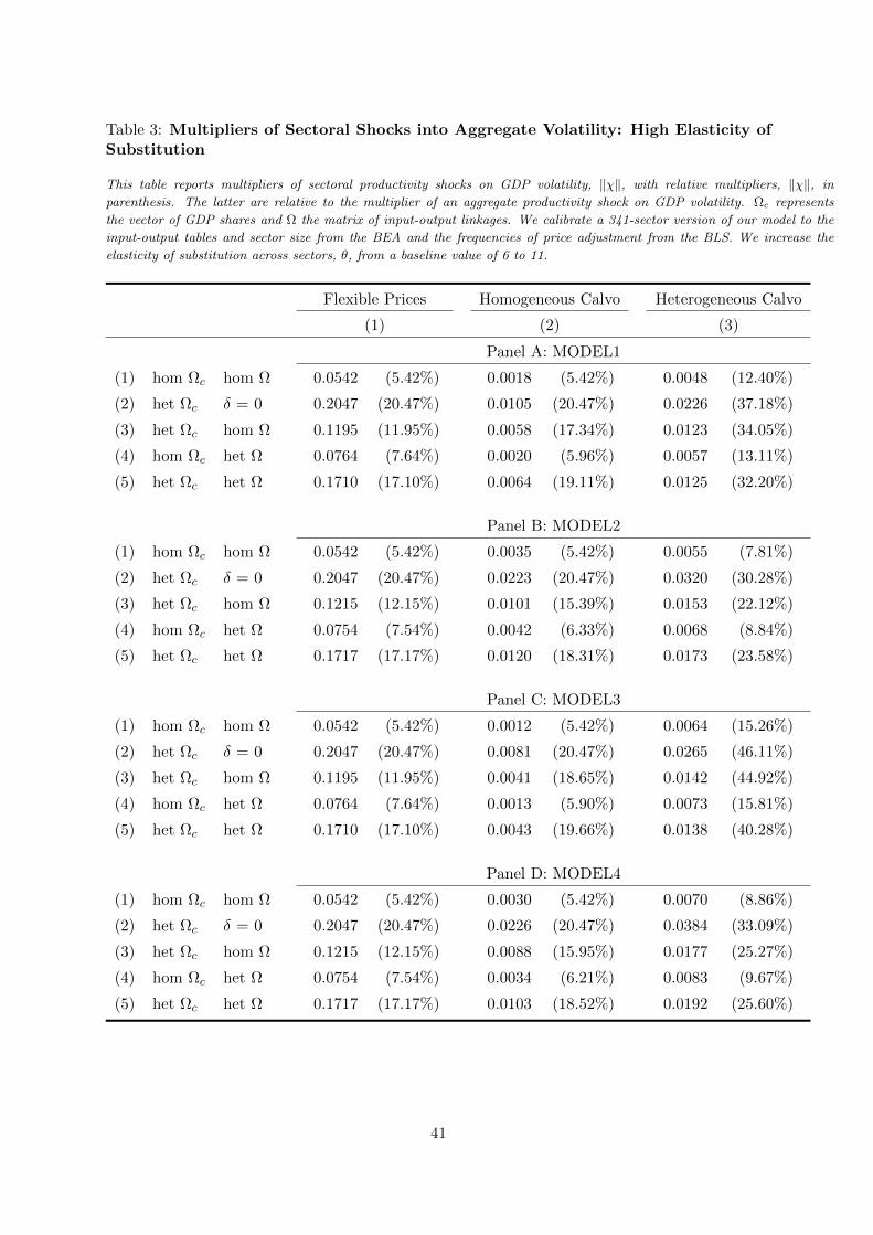
Table 3: Multipliers of Sectoral Shocks into Aggregate Volatility: High Elasticity ofSubstitution

This table reports multipliers of sectoral productivity shocks on GDP volatility, ‖χ‖, with relative multipliers, ‖χ‖, in

parenthesis. The latter are relative to the multiplier of an aggregate productivity shock on GDP volatility. Ωc represents

the vector of GDP shares and Ω the matrix of input-output linkages. We calibrate a 341-sector version of our model to the

input-output tables and sector size from the BEA and the frequencies of price adjustment from the BLS. We increase the

elasticity of substitution across sectors, θ, from a baseline value of 6 to 11.

Flexible Prices Homogeneous Calvo Heterogeneous Calvo

(1) (2) (3)

Panel A: MODEL1

(1) hom Ωc hom Ω 0.0542 (5.42%) 0.0018 (5.42%) 0.0048 (12.40%)

(2) het Ωc δ = 0 0.2047 (20.47%) 0.0105 (20.47%) 0.0226 (37.18%)

(3) het Ωc hom Ω 0.1195 (11.95%) 0.0058 (17.34%) 0.0123 (34.05%)

(4) hom Ωc het Ω 0.0764 (7.64%) 0.0020 (5.96%) 0.0057 (13.11%)

(5) het Ωc het Ω 0.1710 (17.10%) 0.0064 (19.11%) 0.0125 (32.20%)

Panel B: MODEL2

(1) hom Ωc hom Ω 0.0542 (5.42%) 0.0035 (5.42%) 0.0055 (7.81%)

(2) het Ωc δ = 0 0.2047 (20.47%) 0.0223 (20.47%) 0.0320 (30.28%)

(3) het Ωc hom Ω 0.1215 (12.15%) 0.0101 (15.39%) 0.0153 (22.12%)

(4) hom Ωc het Ω 0.0754 (7.54%) 0.0042 (6.33%) 0.0068 (8.84%)

(5) het Ωc het Ω 0.1717 (17.17%) 0.0120 (18.31%) 0.0173 (23.58%)

Panel C: MODEL3

(1) hom Ωc hom Ω 0.0542 (5.42%) 0.0012 (5.42%) 0.0064 (15.26%)

(2) het Ωc δ = 0 0.2047 (20.47%) 0.0081 (20.47%) 0.0265 (46.11%)

(3) het Ωc hom Ω 0.1195 (11.95%) 0.0041 (18.65%) 0.0142 (44.92%)

(4) hom Ωc het Ω 0.0764 (7.64%) 0.0013 (5.90%) 0.0073 (15.81%)

(5) het Ωc het Ω 0.1710 (17.10%) 0.0043 (19.66%) 0.0138 (40.28%)

Panel D: MODEL4

(1) hom Ωc hom Ω 0.0542 (5.42%) 0.0030 (5.42%) 0.0070 (8.86%)

(2) het Ωc δ = 0 0.2047 (20.47%) 0.0226 (20.47%) 0.0384 (33.09%)

(3) het Ωc hom Ω 0.1215 (12.15%) 0.0088 (15.95%) 0.0177 (25.27%)

(4) hom Ωc het Ω 0.0754 (7.54%) 0.0034 (6.21%) 0.0083 (9.67%)

(5) het Ωc het Ω 0.1717 (17.17%) 0.0103 (18.52%) 0.0192 (25.60%)

41

Tab

le4:

Contr

ibu

tion

of

Secto

rsto

Mu

ltip

lier

of

Secto

ral

Sh

ock

son

GD

PV

ola

tility

Th

ista

ble

repo

rts

the

con

trib

uti

on

of

five

mo

stim

port

an

tse

cto

rsto

the

mu

ltip

lier

of

sect

ora

lsh

ocks

on

GD

Pvo

lati

lity

for

MO

DE

L1

an

dth

eid

enti

tyo

fse

cto

rsin

pare

nth

eses

.

Th

ed

iffer

ent

colu

mn

sre

pre

sen

tca

libr

ati

on

sw

hic

hm

atc

hth

efr

equ

ency

of

pri

cea

dju

stm

ents

(λ),

the

dis

trib

uti

on

of

con

sum

pti

on

sha

res

(Ωc),

or

the

act

ua

lin

pu

t-o

utp

ut

ma

trix

(Ω).

11

21

A0

:C

att

lera

nch

ing

an

dfa

rmin

g;1

12

12

0:

Da

iry

catt

lea

nd

mil

kp

rod

uct

ion

;2

11

00

0:

Oil

an

dga

sex

tra

ctio

n;

22

11

00

:E

lect

ric

pow

erge

ner

ati

on

,tr

an

smis

sio

n,

an

d

dis

trib

uti

on

;3

24

11

0:

Pet

role

um

refi

ner

ies;

33

13

1A

:A

lum

ina

refi

nin

ga

nd

pri

ma

rya

lum

inu

mp

rod

uct

ion

;3

31

41

1:

Pri

ma

rysm

elti

ng

an

dre

fin

ing

of

cop

per;

33

61

11

:A

uto

mo

bile

ma

nu

fact

uri

ng;

4A

00

00

:R

eta

iltr

ad

e;4

20

00

0:

Wh

ole

sale

tra

de;

51

70

00

:T

elec

om

mu

nic

ati

on

s;5

2A

00

0:

Mo

net

ary

au

tho

riti

esa

nd

dep

osi

tory

cred

itin

term

edia

tio

n;

53

10

00

:

Rea

les

tate

;6

21

A0

0:

Offi

ces

of

ph

ysic

ian

s,d

enti

sts,

an

do

ther

hea

lth

pra

ctit

ion

ers;

62

20

00

:H

osp

ita

ls

λΩc

λ,

Ωc

Ωλ

,Ω

Ωc,

Ωλ

,Ωc,

Ω

(1)

(2)

(3)

(4)

(5)

(6)

(7)

7.6

2%

(112120)

33.3

3%

(4A

0000)

25.3

3%

(52A

000)

24.5

3%

(420000)

9.8

5%

(211000)

23.2

2%

(4A

0000)

28.6

4%

(52A

000)

6.3

3%

(33131A

)14.4

3%

(420000)

18.7

4%

(420000)

7.6

1%

(531000)

6.6

9%

(112120)

21.9

9%

(531000)

20.7

1%

(420000)

6.3

2%

(331411)

10.8

9%

(531000)

13.5

0%

(211000)

3.6

6%

(221100)

6.2

3%

(324110)

16.8

5%

(420000)

11.4

6%

(324110)

5.9

2%

(211000)

6.6

9%

(621A

00)

11.5

5%

(324110)

3.2

6%

(52A

000)

6.1

5%

(331411)

6.2

5%

(52A

000)

10.4

9%

(4A

0000)

5.4

9%

(1121A

0)

5.7

2%

(622000)

10.7

3%

(336111)

2.9

0%

(4A

0000)

5.7

6%

(1121A

0)

5.5

8%

(517000)

9.2

4%

(336111)

42

Online Appendix:

Price Rigidities and the Granular Origins of AggregateFluctuations

Ernesto Pasten, Raphael Schoenle, and Michael Weber

Not for Publication

I Steady-State Solution and Log-linear System

A. Steady-State Solution

Without loss of generality, set ak = 0. We show below conditions for the existence of a symmetric

steady state across firms in which

Wk = W ,Yjk = Y , Ljk = L, Zjk = Z,Pjk = P for all j, k.

Symmetry in prices across all firms implies

P c = P k = Pk = P

such that, from equations (1), (2), and (10) in the main body of the paper and (13),

Ck = ωckC,

Cjk =1

nkCk,

Zjk(k′)

= ωkk′Z,

Zjk(j′, k′

)=

1

nk′Zjk

(k′).

The vector Ωc ≡ [ωc1, ..., ωcK ]′ represents steady-state sectoral shares in value-added C, Ω =

ωkk′Kk,k′=1 is the matrix of input-output linkages across sectors, and ℵ ≡ [n1, ..., nK ]′ is the

vector of steady-state sectoral shares in gross output Y .

1

It also holds that

C =

K∑k=1

∫=kCjkdj,

Zjk =K∑k′=1

∫=k′

Zjk(j′, k′

)dj′ = Z.

From Walras’ law in equation (19) and symmetry across firms, it holds

Y = C + Z. (A.1)

Walras’ law and results above yield, for all j, k:

Yjk = Cjk +

K∑k′=1

∫=k′

Zj′k′ (j, k) dj′

Y =ωcknk

C +1

nk

(K∑k′=1

nk′ωk′k

)Z,

so ℵ satisfies

nk = (1− ψ)ωck+ ψ

K∑k′=1

nk′ωk′k,

ℵ = (1− ψ)[I − ψΩ′

]−1Ωc,

for ψ ≡ ZY . Note by construction ℵ′ι = 1, which must hold given the total measure of firms is 1.

Steady-state labor supply from equation (7) is

Wk

P= gkL

ϕkC

σ.

In a symmetric steady state, Lk = nkL, so this steady state exists if gk = n−ϕk such that

Wk = W for all k. Thus, steady-state labor supply is given by

W

P= LϕCσ. (A.2)

Households’ budget constraint, firms’ profits, production function, efficiency of production

2

(from equation (15)) and optimal prices in steady state respectively are

CP = WL+ Π (A.3)

Π = PY −WL− PZ (A.4)

Y = L1−δZδ (A.5)

δWL = (1− δ)PZ (A.6)

sP =θ

θ − 1ξW 1−δP δ (A.7)

for ξ ≡ 11−δ

(δ

1−δ

)−δ.

Equation (A.7) solves

W

P=

(θ − 1

θξ

) 11−δ

. (A.8)

This latter result together with equations (A.5), (A.6), and (A.7) solve

Π

P=

1

θY.

Plugging this result in equation (A.4) and using equation (A.1) yields

C =

[1− δ

(θ − 1

θ

)]Y (A.9)

Z = δ

(θ − 1

θ

)Y,

such that ψ ≡ δ(θ−1θ

).

This result and equation (A.7) gives

L =

[δ

(θ − 1

θ

)]− δ1−δ

Y,

where Y solves from this latter result, equations (A.2), (A.9) and (A.8):

Y =

(θ − 1

θξ

) 1(1−δ)(σ+ϕ)

[δ

(θ − 1

θ

)] δϕ(1−δ)(σ+ϕ)

[1− δ

(θ − 1

θ

)]− σσ+ϕ

.

3

B. Log-linear System

B.1 Aggregation

Aggregate and sectoral consumption (interpreted as value-added) given by equations (1) and (2)

are

ct =K∑k=1

ωckckt, (A.10)

ckt =1

nk

∫=kcjktdj.

Aggregate and sectoral production of intermediate inputs are given by

zt =K∑k=1

nkzkt, (A.11)

zkt =1

nk

∫=kzjktdj,

where (10) and (13) imply that zjk =∑K

r=1 ωkrzjk (r) and zjk (r) = 1nr

∫=r zjk (j′, r) dj′.

Sectoral and aggregate prices are given from equations (4), (6), and (12),

pkt =

∫=kpjkdj for k = 1, ...,K

pct =K∑k=1

ωckpkt,

pkt =K∑k′=1

ωkk′pk′t.

Aggregation of labor is

lt =

K∑k=1

lkt, (A.12)

lkt =

∫=kljktdj.

4

B.2 Demands

Households’ demand for sectors and goods in equations (3) and (5) for all k = 1, ...,K become

ckt − ct = η (pct − pkt) , (A.13)

cjkt − ckt = θ (pkt − pjkt) .

In turn, firm jk’s demand for sectors and goods in equation (11) and (14) for all k, r =

1, ...,K,

zjkt(k′)− zjkt = η

(pkt − pk′t

), (A.14)

zjkt(j′, k′

)− zjkt

(k′)

= θ(pk′t − pj′k′t

).

Firms’ gross output satisfies Walras’ law,

yjkt = (1− ψ) cjkt + ψK∑k′=1

∫=k′

zj′k′t (j, k) dj′. (A.15)

Total gross output follows from the aggregation of equations (19),

yt = (1− ψ) ct + ψzt. (A.16)

B.3 IS and labor supply

The household Euler equation in equation (8) becomes

ct = Et [ct+1]− σ−1it −

(Et[pct+1

]− pt

).

The labor supply condition in equation (7) is

wkt − pct = ϕlkt + σct. (A.17)

B.4 Firms

Production function:

yjkt = akt + (1− δ) ljkt + δzjkt (A.18)

5

Efficiency condition:

wkt − pkt = zjkt − ljkt (A.19)

Marginal costs:

mckt = (1− δ)wkt + δpkt − akt (A.20)

Optimal reset price:

p∗kt = (1− αkβ)mckt + αkβEt[p∗kt+1

]Sectoral prices:

pkt = (1− αk) p∗kt + αkpkt−1

B.5 Taylor rule:

it = φπ(pct − pct−1

)+ φcct

6

II Solution of Key Equations in Section III

A. Solution of Equation (25)

Setting σ = 1 and ϕ = 0 in equation (A.17) yields

wkt = ct + pct = 0,

where the equality follows from the assumed monetary policy rule, so equation (A.20) becomes

mckt = δpkt − akt.

Here, sectoral prices for all k = 1, ...,K are governed by

pkt = (1− λk)mckt

= δ (1− λk) pkt − (1− λk) akt,

which in matrix form solves

pt = − [I− δ (I− Λ) Ω]−1 (I− Λ) at.

pt ≡ [p1t, ..., pKt]′ is the vector of sectoral prices, Λ is a diagonal matrix with the vector

[λ1, ..., λK ]′ in its diagonal, Ω is the matrix of input-output linkages, and at ≡ [a1t, ..., aKt]′

is the vector of realizations of sectoral technology shocks.

The monetary policy rule implies ct = −pct , so

ct =(I− Λ′

) [I− δ

(I− Λ′

)Ω′]−1

Ω′cat.

Solution of Equation (28)

Setting σ = 1 and ϕ > 0 in (A.17) yields

wkt = ϕlskt + ct + pct = ϕldkt,

which follows from the assumed monetary policy rule.

Labor demand is obtained from the production function in equation (A.18), the efficiency

7

condition for production in equation (A.19), and the aggregation of labor in equation (A.12):

ldkt = ykt − akt − δ(wkt − pkt

).

ykt follows from equations (A.10), (A.11), (A.13), (A.14), and (A.15):

ykt = yt − η

(pkt −

[(1− ψ) pct + ψ

K∑k=1

nkpkt

]),

where

pt ≡K∑k=1

nkpkt =

K∑k=1

ζkpkt,

with ζk ≡∑K

k′=1 nk′ωk′k.

To solve for yt, we use equations (A.11), (A.12), (A.16) and yt =∑K

k=1

∫=k yjktdj to get

yt = ct + ψ

[Γcct − Γp (pt − pct)− Γa

K∑k=1

nkakt

],

where Γc ≡ (1−δ)(1+ϕ)(1−ψ)+ϕ(δ−ψ) ,Γp ≡

1−δ(1−ψ)+ϕ(δ−ψ) , Γa ≡ 1+ϕ

(1−ψ)+ϕ(δ−ψ) .

Putting together all these equations, sectoral wages solve

wkt =ϕ

1 + δϕ

(1 + ψΓc) ct − akt − ψΓa∑K

k′=1 nk′ak′t

[(1− ψ) η + ψΓp] pct + ψ (η − Γp) pt + δpkt − ηpkt

.With this expression, the solution to equation (28) follows the same steps as the solution

to equation (25).

8

III The Network Effect, the Granular Effect, and Price Rigidity

We find in Section VI across calibrations that (i) heterogeneity in price stickiness alone can

generate large aggregate fluctuations from idiosyncratic shocks, (ii) homogeneous input-output

linkages mute the granular effect relative to an economy without intermediate input use, and (iii)

introducing heterogeneous price stickiness across sectors in an economy with sectors of different

sizes but homogeneous input-output linkages increases the size of the relative multipliers.

Consider the economy of Section III with sectors of potentially different sizes, input-output

linkages, and price rigidities. In this general case, the vector of multipliers up to second-order

terms has elements

χk ≥ (1− λk)[ωck + δdk + δ2qk

]. (A.21)

As before, ωck denotes the size of sector k, dk the generalized outdegree of sector k, and qk

the generalized second-order outdegree of sector k:

dk ≡K∑k′=1

ωck′ (1− λk′)ωk′k, (A.22)

qk =K∑k′=1

dk′ (1− λk′)ωk′k.

These two terms embody the effects of heterogeneity of GDP shares, I/O linkages, and price

rigidity across sectors. The multiplier of idiosyncratic shocks as in the previous derivations

equals ‖χ‖2 =√∑K

k=1 χ2k, and

∑Kk=1 χk represents the multiplier of an aggregate shock.

Lemma 5 If input-output shares and sector sizes are homogeneous across sectors, that is,

ωck = ωkk′ = 1/K for all k, k′, but price stickiness λk is heterogeneous, then the multiplier

of idiosyncratic shocks is

‖χ‖2 =1

K(1− δ

(1− λ

))√√√√ K∑

k=1

(1− λk)2,

where λ ≡ 1K

∑Kk=1 λk. The multiplier is increasing in the dispersion of price stickiness across

sectors. The aggregate multiplier is invariant to allowing for price dispersion. Thus, the

multiplier of sectoral shocks relative to aggregate shocks is increasing in the dispersion of price

rigidity.

Proof. See Online Appendix.

9

The intuition for the previous proposition follows exactly as in Section III B.. The

next proposition considers the case in which only input-output linkages are restricted to be

homogeneous:

Lemma 6 If input-output linkages are homogeneous across sectors, that is, ωkk′ = 1/K for

all k, k′, but sector size ωck is unrestricted and prices are frictionless (λk = 0), then given

var(ωck) ≥ var(1/K), the multiplier of sectoral shocks relative to the aggregate shock multiplier,

√∑Kk=1

(ωck + δ/K

1−δ

)2

(1− δ)−1 ≤

√√√√ K∑k=1

ω2ck,

is smaller than when input-output linkages are shut down (δ = 0), ceteris paribus.

Proof. See Online Appendix.

Allowing for price stickiness (λk > 0) is an important case in the calibrations. We study this

case next. Relative to the previous proposition, we find that the introduction of heterogeneous

price rigidity leads to an overall increase in the relative multiplier.

Lemma 7 If input-output linkages are homogeneous across sectors, that is, ωkk′ = 1/K for all

k, k′, but sector size ωck is unrestricted, and price rigidity is heterogeneous (λk > 0), then given

λ ≡ 1K

∑Kk=1 λk, λ ≡ 1

K

∑Kk=1 ωckλk the multiplier of idiosyncratic shocks relative to aggregate

shocks,

‖χ‖2K∑k=1

χk

=

√√√√∑Kk=1 (1− λk)2

(ωck +

δ(

1−λ)/K

1−δ(1−λ)

)2

(1− λ

)/[1− δ

(1− λ

)] ,

is (1) increasing in the simple and weighted average of heterogeneous price rigidity across sectors,

1−λ, and 1−λ, (2) increasing in the covariance of price rigidity and sector size, cov((1−λk, ωck),

and (3) increasing in the dispersion of sectoral price flexibility, λk.

Proof. See Online Appendix.

The first effect (1) is an effect due to the average degree of price rigidity in the economy.

The last two effects (2) and (3) capture the effect of heterogeneity in the interaction with sector

size and the dispersion of price flexibility.

10

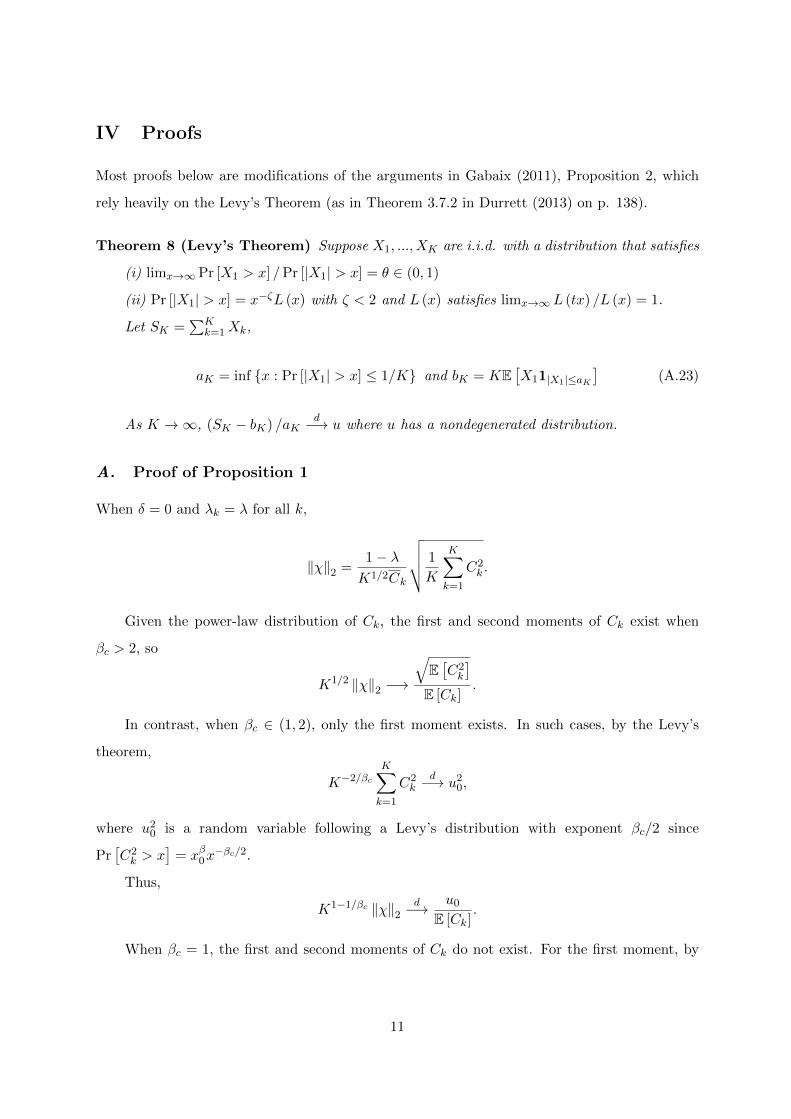
IV Proofs

Most proofs below are modifications of the arguments in Gabaix (2011), Proposition 2, which

rely heavily on the Levy’s Theorem (as in Theorem 3.7.2 in Durrett (2013) on p. 138).

Theorem 8 (Levy’s Theorem) Suppose X1, ..., XK are i.i.d. with a distribution that satisfies

(i) limx→∞ Pr [X1 > x] /Pr [|X1| > x] = θ ∈ (0, 1)

(ii) Pr [|X1| > x] = x−ζL (x) with ζ < 2 and L (x) satisfies limx→∞ L (tx) /L (x) = 1.

Let SK =∑K

k=1Xk,

aK = inf x : Pr [|X1| > x] ≤ 1/K and bK = KE[X11|X1|≤aK

](A.23)

As K →∞, (SK − bK) /aKd−→ u where u has a nondegenerated distribution.

A. Proof of Proposition 1

When δ = 0 and λk = λ for all k,

‖χ‖2 =1− λK1/2Ck

√√√√ 1

K

K∑k=1

C2k .

Given the power-law distribution of Ck, the first and second moments of Ck exist when

βc > 2, so

K1/2 ‖χ‖2 −→

√E[C2k

]E [Ck]

.

In contrast, when βc ∈ (1, 2), only the first moment exists. In such cases, by the Levy’s

theorem,

K−2/βc

K∑k=1

C2k

d−→ u20,

where u20 is a random variable following a Levy’s distribution with exponent βc/2 since

Pr[C2k > x

]= xβ0x

−βc/2.

Thus,

K1−1/βc ‖χ‖2d−→ u0

E [Ck].

When βc = 1, the first and second moments of Ck do not exist. For the first moment, by

11

Levy’s theorem, (Ck − logK

) d−→ g,

where g is a random variable following a Levy distribution.

Since the second moment is equivalent to the result above,

(logK) ‖χ‖2d−→ u′.

B. Proof of Proposition 2

Let λk and Ck be two independent random variables distributed as specified in the Proposition,

the counter-cumulative distribution of zk = (1− λk)Ck is given by

fZ (z) =

∫ z/y0

zfCk (z/y) f1−λk (y) dy,

which follows as Pareto distribution with shape parameter βc. The proof of the Proposition

then follows the proof of Proposition 1 for

‖χ‖2 =1

K1/2Ck

√1

Kz2k. (A.24)

C. Proof of Proposition 3

As specified in the proposition, λk and Ck are related through Zk = (1− λk)Ck = φC1+µk .

When µ < 0, Zk is distributed Pareto with shape parameter βc/ (1 + µ). Proceeding similarly

to the proof of Proposition 1, when βc > max 1, 2 (1 + µ), both E[Z2k

]and E [Ck] exist, so

vc ∼ v/K1/2. When βc ∈ (1,max 1, 2 (1 + µ)), E [Ck] exist but E[Z2k

]does not.

Applying Levy’s theorem,

K−2(1+µ)/βc

K∑k=1

Z2k

d−→ u2.

Thus, vc ∼ u1K1−(1+µ)/β v.

When βc = 1, the last result also holds. But now E [Ck] does not exist. As in Proposition 1,(1K

K∑k=1

Ck − logK

)d−→ g. Thus, if µ ∈ [−1/2, 0], vc ∼ u2

K−µ logKv, whereas if µ ∈ (−1,−1/2),

vc ∼ u2K1/2 logK

v.

The proposition for µ < 0 is then obtained by rearranging terms.

12

When µ > 0, Zk is distributed piece-wise Pareto such that

Pr [Zk ≥ z] =

xβc0 z−βc for z > φ−2/µ

z−βc/(1+µ)0 z−βc/(1+µ) for z ∈

[z2

0 , φ−2/µ

].

We now follow the same steps as in the proof of Proposition 1. When βc > 2 (1 + µ), E[Z2k

]and E [Ck] exist, so vc ∼ v/K1/2. When βc ∈ (1, 2 (1 + µ)), E [Ck] exists but E

[Z2k

]does not.

Applying Levy’s theorem,

1

aK

K∑k=1

Z2k

d−→ u2,

where

aK =

x20K

2/βc for K > K∗

z20K

2(1+µ)/βc for K ≤ K∗

for K∗ ≡ x−βc0 φ−βc/µ. Thus, vc ∼ u1

K1− 1+1K≤K∗µ

βc

v for some random variable u1.

When βc = 1,

(1K

K∑k=1

Ck − logK

)d−→ g, so now vc ∼ u2

K−1K≤K∗µ logKv for some random

variable u2, completing the proof.

D. Proof of Proposition 4

When δ ∈ (0, 1), λk = λ for all k, and Ωc = 1K ι, we know from equation XX that

‖χ‖2 ≥ 1− λK

√√√√ K∑k=1

[1 + δ′dk + δ′2qk]2

≥ (1− λ)

√√√√1 + 2δ′ + 2δ′2

K+δ′2

K2

K∑k=1

[d2k + 2δ′dkqk + δ′2q2

k

].

Following the same argument as in Proposition 2,

K−2/βd

K∑k=1

d2k −→ u2

d,

K−2/βq

K∑k=1

q2k −→ u2

q ,

K−1/βz

K∑k=1

dkqk −→ u2z,

13

where u2d, u

2q and u2

z are random variables. Thus, if βz ≥ 2 min βd, βq,

vc ≥u3

K1−1/minβd,βqv

where u23 is a random variable.

E. Proof of Proposition 5

Analogous to the proof of Proposition 4.

F. Proof of Proposition 5

This proposition follows from the dispersion of price stickiness across sectors entirely analogously

as in the discussion of the granularity effect in Section III B.].

G. Proof of Proposition 6

This proposition follows entirely analogously to the previous ones. Note that the inequality

holds if var(ωck ≥ 1/K.

H. Proof of Proposition 7

This follows directly from the given expression, as well as from Jensen’s Inequality.

14

V Distribution of the Frequency of Price Changes

Here, we report the shape parameters of the power law distribution for the frequencies of price

adjustments following Gabaix and Ibragimov (2011). To do so, we compute the OLS estimator

of the empirical log-counter cumulative distribution on the log sequence of the variables using

the data in the upper 20% tail. The shape parameter of the sectoral distribution of frequency

of price changes is 2.5773 (st dev 0.4050); that is, the distribution of the frequency of price

adjustment is not fat-tailed.

15

Table A.1: Multipliers of Sectoral Shocks into Aggregate Volatility: with construction

This table reports multipliers of sectoral productivity shocks on GDP volatility, ‖χ‖, with relative multipliers, ‖χ‖, in

parenthesis. The latter are relative to the multiplier of an aggregate productivity shock on GDP volatility. Ωc represents

the vector of GDP shares and Ω the matrix of input-output linkages. We calibrate a 341-sector version of our model to the

input-output tables and sector size from the BEA and the frequencies of price adjustment from the BLS.

Flexible Prices Homogeneous Calvo Heterogeneous Calvo

(1) (2) (3)

Panel A: MODEL1

(1) hom Ωc hom Ω 0.0535 (5.35%) 0.0016 (5.35%) 0.0044 (11.94%)

(2) het Ωc δ = 0 0.1922 (19.22%) 0.0093 (19.22%) 0.0190 (32.57%)

(3) het Ωc hom Ω 0.1067 (10.67%) 0.0047 (16.01%) 0.0096 (29.50%)

(4) hom Ωc het Ω 0.0793 (7.93%) 0.0018 (6.02%) 0.0053 (12.89%)

(5) het Ωc het Ω 0.1604 (16.04%) 0.0053 (17.88%) 0.0096 (27.87%)

Panel B: MODEL2

(1) hom Ωc hom Ω 0.0535 (5.35%) 0.0029 (5.35%) 0.0049 (7.93%)

(2) het Ωc δ = 0 0.1922 (19.22%) 0.0197 (19.22%) 0.0263 (25.84%)

(3) het Ωc hom Ω 0.1100 (11.00%) 0.0078 (14.49%) 0.0114 (19.72%)

(4) hom Ωc het Ω 0.0773 (7.73%) 0.0034 (6.31%) 0.0061 (8.95%)

(5) het Ωc het Ω 0.1614 (16.14%) 0.0093 (17.27%) 0.0125 (20.78%)

Panel C: MODEL3

(1) hom Ωc hom Ω 0.0535 (5.35%) 0.0010 (5.35%) 0.0058 (14.83%)

(2) het Ωc δ = 0 0.1922 (19.22%) 0.0070 (19.22%) 0.0227 (41.68%)

(3) het Ωc hom Ω 0.1067 (10.67%) 0.0032 (17.44%) 0.0112 (40.56%)

(4) hom Ωc het Ω 0.0793 (7.93%) 0.0011 (5.93%) 0.0067 (15.68%)

(5) het Ωc het Ω 0.1604 (16.04%) 0.0034 (18.47%) 0.0107 (36.12%)

Panel D: MODEL4

(1) hom Ωc hom Ω 0.0535 (5.35%) 0.0027 (5.35%) 0.0069 (8.61%)

(2) het Ωc δ = 0 0.1922 (19.22%) 0.0195 (19.22%) 0.0319 (28.39%)

(3) het Ωc hom Ω 0.1149 (11.49%) 0.0076 (15.05%) 0.0148 (22.02%)

(4) hom Ωc het Ω 0.0747 (7.47%) 0.0031 (6.13%) 0.0082 (9.41%)

(5) het Ωc het Ω 0.1628 (16.28%) 0.0089 (17.48%) 0.0157 (22.27%)

16