NBER WORKING PAPER SERIES

CAPITAL MARKETS IN CHINA AND BRITAIN, 18TH AND 19TH CENTURY: EVIDENCE FROM GRAIN PRICES

Wolfgang KellerCarol H. Shiue

Xin Wang

Working Paper 21349http://www.nber.org/papers/w21349

NATIONAL BUREAU OF ECONOMIC RESEARCH1050 Massachusetts Avenue

Cambridge, MA 02138July 2015, Revised May 2018

We thank Howard Bodenhorn, Stephen Broadberry, Edmund Cannon, Kris Mitchener, Kevin O’Rourke, Sevket Pamuk, and Jeff Williamson, as well as participants at CEPR/CAGE Venice, the Third Quantitative Economic History workshop in Beijing, and the World Economic History conference in Kyoto for comments. Thanks to Edmund Cannon, Wang Yeh-Chien, Nathan Nunn, Jeff Williams, and Brian Wright for research support. William Ridley and Austin Smith performed excellent research assistance. NSF support under grant SES 1124426 is gratefully acknowledged. Part of this research was done when Keller and Shiue were National Fellows at the Hoover Institution in Stanford, which they thank for its hospitality. The views expressed herein are those of the authors and do not necessarily reflect the views of the National Bureau of Economic Research.

NBER working papers are circulated for discussion and comment purposes. They have not been peer-reviewed or been subject to the review by the NBER Board of Directors that accompanies official NBER publications.

© 2015 by Wolfgang Keller, Carol H. Shiue, and Xin Wang. All rights reserved. Short sections of text, not to exceed two paragraphs, may be quoted without explicit permission provided that full credit, including © notice, is given to the source.

Capital Markets in China and Britain, 18th and 19th Century: Evidence from Grain Prices Wolfgang Keller, Carol H. Shiue, and Xin WangNBER Working Paper No. 21349July 2015, Revised May 2018JEL No. G12,N10,N13,N25,O10

ABSTRACT

Based on the most comprehensive grain prices available, we employ a storage model to estimate consistent interest rates and compare capital market development in Britain and China. Interest rates for Britain were lower than China’s on average by about three percentage points from 1770 to 1860. Regional capital market integration in the Yangzi Delta comes close to the British average at distances below 200 kilometers, but at larger distances interest rate correlations in Britain are twice those of the Delta, and three or more times as high as elsewhere in China. Overall, our results suggest capital market divergence at an early date.

Wolfgang KellerDepartment of EconomicsUniversity of Colorado, BoulderBoulder, CO 80309-0256and NBERWolfgang.Keller@colorado.edu

Carol H. ShiueDepartment of EconomicsUniversity of Colorado at BoulderBoulder, CO 80309and NBERcarol.shiue@colorado.edu

Xin WangInstitute of New Structural EconomicsPeking UniversityBeijing 100871Chinaxin.wang@nsd.pku.edu.cn

2

I. Introduction

Why did modern economic growth begin in Northwest Europe, and not in China? Some

time ago Kenneth Pomeranz addressed this classic question in The Great Divergence: China,

Europe, and the Making of the Modern World (Pomeranz 2000), emphasizing the similarities

across Asia and European in factors responsible for growth.1 Despite the progress being

made over the last years, there is no consensus yet on the cause for the Great Divergence.

Nearly everyone would agree, however, that a relatively low interest rate indicates not only

the abundance of capital but also low levels of risk in capital market transactions (North

and Weingast 1989). Perhaps most importantly, well-developed capital markets allow

surplus to flow to the project with the highest return.2 They were, for example, an

important factor for early growth in Europe and North America (Davis 1965, Sylla 1969,

Rousseau 2003, Hoffman, Postel-Vinay, and Rosenthal 2011). But how different was capital

market development in China in the late 18th and early 19th centuries compared to Western

regions? Most accounts contrast thick, developed capital markets and low interest rates in

Europe against the less developed Chinese markets starved for capital, but one should not

accept these conclusions at face value (Rosenthal and Wong 2011).3 In this paper, we

circumvent the lack of data on comparable interest rates by using a storage model with

local grain price information in order to shed new light on capital market development in

Britain and China between 1770 and 1860.

Specifically, the price for a stored commodity must compensate for the cost of storage,

of which the interest rate is a key determinant (Hotelling 1931, Working 1933, 1949,

Kaldor 1939). Holding on to a stored commodity is more expensive the more scarce are the

funds—the higher the interest rate—and the higher is the risk. If there is a ten percent

chance that the commodity is stolen by bandits (or expropriated by the government), the

storer will demand a ten percent higher forward price to compensate for the risk of losing

1 The lasting influence of Pomeranz (2000) is evidenced by the special session “Assessing Kenneth Pomeranz Great Divergence: A Forum” ten years after publication, Forum (2011). 2 Allen (2009) emphasizes that developed capital markets may have given Europe a relatively strong incentive for capital deepening, leading to growth. On the link between capital market development and economic growth, see Bagehot (1857), Schumpeter (1911), and Gurley and Shaw (1955), as well as more recently Rousseau and Wachtel (1998), Rousseau (1999), and Mitchener and Ohnuki (2007). 3 In particular, the lack of comparable interest rates—for which investment, borrower, security, risk, maturity, etc.—can produce major challenges. For a review and broader discussion, see Rosenthal and Wong (2011).

3

the commodity. We estimate comparable regional interest rates for Britain and China.

Because comparable data on interest rates are not available, we examine interest rates from

the point of view of an asset held over time, as in McCloskey and Nash (1984). However, we

go further than that. Building on these interest rates we shed new light on the

development of regional capital markets in Britain and China by studying the integration of

capital markets during the crucial years of economic divergence, from 1770 to 1860.1

There are several major findings. We find, first, that our interest rate estimates are

typically lower in Britain than in China, with averages of 5.4% versus 8.4% per year,

respectively. Second, we find that British capital markets were substantially more

integrated than capital markets in China. Bilateral correlations for regions within the

Yangzi Delta come close to the British average at distances below 200 kilometers, but at

larger distances interest rate correlations in Britain are twice those of the Delta. Outside of

the Yangzi Delta regional interest rate correlations are often less than one-third the British

average. And while Britain increased its advantage over China during the period of 1770 to

1860, already by the end of the 18th century there was a substantial gap in capital market

integration between the two countries.

We contribute to a large literature in comparative development that seeks to examine

the divergence between China and Europe and the larger lessons on the causes of growth

and development (Needham 1969, Pomeranz 2000, Rosenthal and Wong 2011, Lin 2014).

Considerable progress has been made in terms of documenting the Great Divergence

through income and national accounts studies (Allen, Bassino, Ma, Moll-Murata, and van

Zanden 2011, Broadberry, Guan, and Li 2014). Nevertheless, explaining the Great

Divergence has been a greater challenge. While numerous factors have been considered

there is little research on capital market development.2 By providing a comparable set of

1 A parallel paper has shown that this storage approach works well in uncovering differences in capital market development in other early 19th century economies. Matching bank interest rates and grain-price based rates for several regions in the U.S. during 1815-1855, Keller, Shiue, and Wang (2018) find that the correlation of average bank and grain rates is high. 2 For an introduction of the Great Divergence debate, see Forum (2011) as well as Brandt, Ma, and Rawski (2014). Goetzmann et al. (2007) discusses the 19th and 20th century formation of a national stock market, and the process of the securitization of assets of Chinese firms and government debt. Work referring to capital markets includes Li and van Zanden (2013) who report that in the late 18th and early 19th centuries annual interest rates in the Yangzi Delta were between 5% (commercial loans, mortgages) and 25% or higher

4

regional interest rates that is analyzed to study capital market integration in Britain and

China we provide a new empirical grounding for explanations of the Great Divergence that

refer to capital markets.

Our finding that Britain’s capital market integration was much higher than China’s,

already by the late 18th century, provides initial evidence that capital market development

plays an important role in the Great Divergence. This finding differs markedly from an

earlier paper that demonstrated there was only small gap in the efficiency of China’s

commodity markets relative to those in Europe (Shiue and Keller 2007).1 The difference

reflects the fact that the within-year price dynamics underlying this study of capital

markets provide very different information compared to the essentially static comparison

of commodity market integration across regions for a given period.

Second, the paper contributes to the quantitative study of capital market development.

Little is known on capital market integration, either historically or on today’s less-

developed countries (19th century U.S. and Japan are exceptions, see Davis 1965,

Bodenhorn and Rokoff 1992, and Mitchener and Ohnuki 2007, 2009, respectively).2 A key

advantage of our storage approach is that it sheds light on capital market development

prior to the 19th century. While we do not study the causal impact of capital markets, our

analysis opens up new lines of research on industrialization and growth that do not require

information on interest rates charged by formal financial institutions. This is useful

because by the time these have been established, numerous other factors associated with

industrialization have also occurred, making it difficult to assess the causal role of finance.3

The remainder of the paper is as follows. Section 2 introduces a simple storage cost

approach that we employ to infer interest rates from monthly grain prices. We also discuss

our measures of capital market development to compare China with Britain. Section 3

describes our regional grain price data, as well as supplementary information, in particular

historical weather data. Section 4 contains our main empirical results. First we compare

regional interest rates, followed by studying capital market integration in Britain and China, (pawnshop rates), compared to 3-5% (commercial loans, mortgages, and government bonds) in the Netherlands. 1 See also Studer (2008) for a comparative analysis of India. 2 Good (1977) and Brunt and Cannon (2009) study 19th century Austria and England, respectively. 3 Keller and Shiue (2017) employ the storage approach to study the causal effect of capital market development brought about by Western colonial institutions in China.

5

where the latter includes a special analysis of the Yangzi Delta. We cap the empirical results

section with a number of important robustness checks in section 4.5, before turning to a

concluding discussion in section 5.

2. Empirical Framework

2. 1 Grain Prices, Storage Costs, and Capital Markets

Could underdeveloped capital markets, due to perhaps a general lack of capital as well

as risks in capital transactions, have contributed to the Great Divergence? While there are

many ways to approach this question, we focus on the level of regional interest rates and

the extent of capital market integration, both of which govern the extent to which capital

surplus can be allocated to the project with the highest return. Capital market integration

may be simply measured by the degree to which interest rates in different regions co-move

with each other. The stronger are these co-movements, the more highly integrated are the

capital markets in that area (e.g., Mitchener and Ohnuki 2007, 2009).

In practice, the key difficulty in carrying out this analysis is that strictly comparable

interest rates are generally not available for across regions for Britain and China before the

19th century.1 This is because the interest rate charged in any particular transaction

depends on a multitude of characteristics—of the borrower, the lender, the type of project,

its maturity, specific risk, time of year, whether there was a security, etc.—and there are

typically not enough transactions of a particular type to allow valid comparisons. Thus,

even though there are numerous and scattered interest rates in historical sources for China,

they are not suitable for systematic comparisons because crucial transaction details are

missing (Pomeranz 1993, 32). Likewise, the absence of comparable regional interest rates

even with Britain during the 18th century is the reason why researchers studying the

emergence of a national English capital market have had to resort to relating the interest

rate in London to the number of real estate transactions in the regions of England

(Buchinsky and Polak 1993). Thus, the first step in our analysis is to construct a set of

comparable regional interest rates, to which we turn now.

1 A recent compilation of historical interest rates for China is Tang (2016).

6

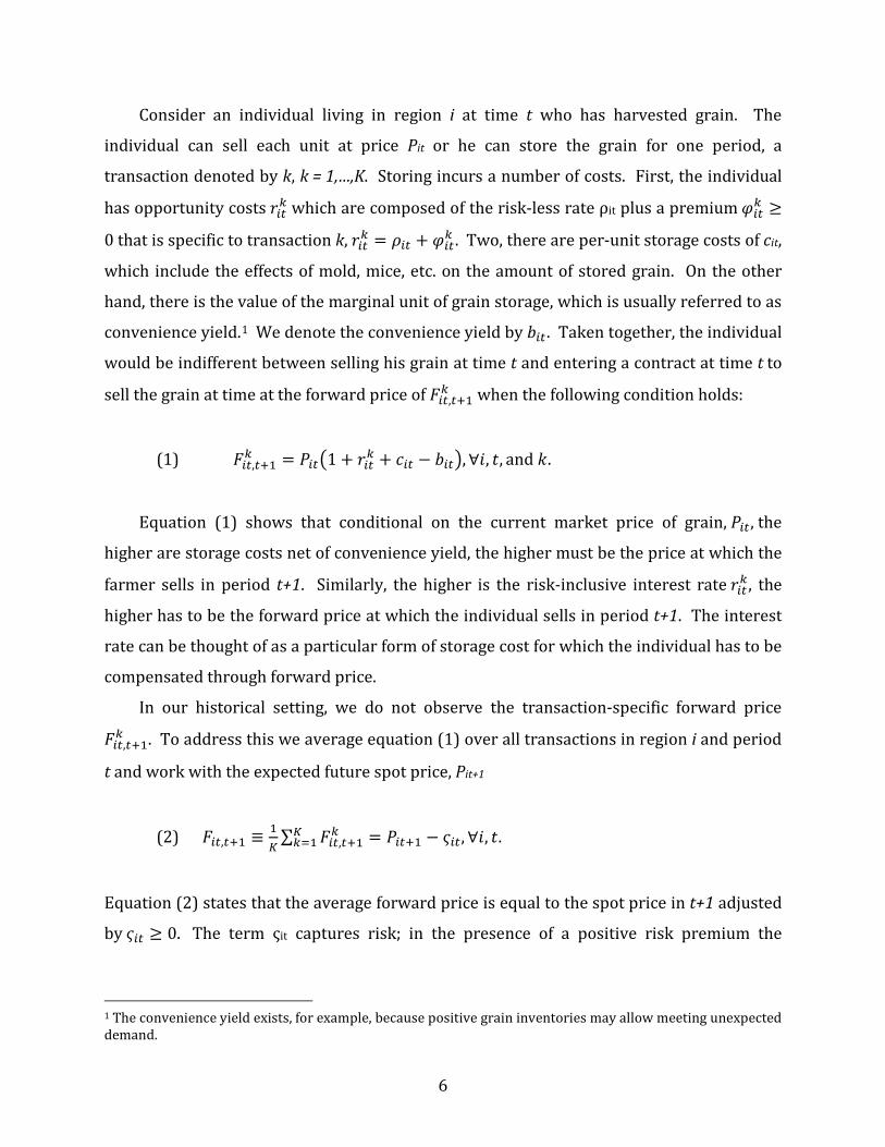
Consider an individual living in region i at time t who has harvested grain. The

individual can sell each unit at price Pit or he can store the grain for one period, a

transaction denoted by k, k = 1,…,K. Storing incurs a number of costs. First, the individual

has opportunity costs 𝑟𝑟𝑖𝑖𝑖𝑖𝑘𝑘 which are composed of the risk-less rate ρit plus a premium 𝜑𝜑𝑖𝑖𝑖𝑖𝑘𝑘 ≥

0 that is specific to transaction k, 𝑟𝑟𝑖𝑖𝑖𝑖𝑘𝑘 = 𝜌𝜌𝑖𝑖𝑖𝑖 + 𝜑𝜑𝑖𝑖𝑖𝑖𝑘𝑘 . Two, there are per-unit storage costs of cit,

which include the effects of mold, mice, etc. on the amount of stored grain. On the other

hand, there is the value of the marginal unit of grain storage, which is usually referred to as

convenience yield.1 We denote the convenience yield by 𝑏𝑏𝑖𝑖𝑖𝑖. Taken together, the individual

would be indifferent between selling his grain at time t and entering a contract at time t to

sell the grain at time at the forward price of 𝐹𝐹𝑖𝑖𝑖𝑖,𝑖𝑖+1𝑘𝑘 when the following condition holds:

(1) 𝐹𝐹𝑖𝑖𝑖𝑖,𝑖𝑖+1𝑘𝑘 = 𝑃𝑃𝑖𝑖𝑖𝑖�1 + 𝑟𝑟𝑖𝑖𝑖𝑖𝑘𝑘 + 𝑐𝑐𝑖𝑖𝑖𝑖 − 𝑏𝑏𝑖𝑖𝑖𝑖�,∀𝑖𝑖, 𝑡𝑡, and 𝑘𝑘.

Equation (1) shows that conditional on the current market price of grain, 𝑃𝑃𝑖𝑖𝑖𝑖, the

higher are storage costs net of convenience yield, the higher must be the price at which the

farmer sells in period t+1. Similarly, the higher is the risk-inclusive interest rate 𝑟𝑟𝑖𝑖𝑖𝑖𝑘𝑘, the

higher has to be the forward price at which the individual sells in period t+1. The interest

rate can be thought of as a particular form of storage cost for which the individual has to be

compensated through forward price.

In our historical setting, we do not observe the transaction-specific forward price

𝐹𝐹𝑖𝑖𝑖𝑖,𝑖𝑖+1𝑘𝑘 . To address this we average equation (1) over all transactions in region i and period

t and work with the expected future spot price, Pit+1

(2) 𝐹𝐹𝑖𝑖𝑖𝑖,𝑖𝑖+1 ≡1𝐾𝐾∑ 𝐹𝐹𝑖𝑖𝑖𝑖,𝑖𝑖+1

𝑘𝑘𝐾𝐾𝑘𝑘=1 = 𝑃𝑃𝑖𝑖𝑖𝑖+1 − 𝜍𝜍𝑖𝑖𝑖𝑖,∀𝑖𝑖, 𝑡𝑡.

Equation (2) states that the average forward price is equal to the spot price in t+1 adjusted

by 𝜍𝜍𝑖𝑖𝑖𝑖 ≥ 0. The term ςit captures risk; in the presence of a positive risk premium the

1 The convenience yield exists, for example, because positive grain inventories may allow meeting unexpected demand.

7

forward price will be below the expected future spot price. Furthermore, we define the

adjusted storage cost �̃�𝑐𝑖𝑖𝑖𝑖 as

(3) �̃�𝑐𝑖𝑖𝑖𝑖 ≡ 𝑐𝑐𝑖𝑖𝑖𝑖 − 𝑏𝑏𝑖𝑖𝑖𝑖 + 𝜍𝜍𝑖𝑖𝑖𝑖𝑃𝑃𝑖𝑖𝑖𝑖

,∀𝑖𝑖, 𝑡𝑡.

Substituting equations (2) and (3) into equation (1) yields

(1’) 𝑃𝑃𝑖𝑖𝑖𝑖+1 = 𝑃𝑃𝑖𝑖𝑖𝑖(1 + 𝑟𝑟𝑖𝑖𝑖𝑖 + �̃�𝑐𝑖𝑖𝑖𝑖),∀𝑖𝑖, 𝑡𝑡,

where 𝑟𝑟𝑖𝑖𝑖𝑖 = 1𝐾𝐾∑ 𝑟𝑟𝑖𝑖𝑖𝑖𝑘𝑘𝐾𝐾𝑘𝑘=1 . Equation (1’) shows that for a given price Pit, the higher is the risk-

inclusive interest rate 𝑟𝑟𝑖𝑖𝑖𝑖, the higher is Pit+1.

To provide further intuition, we simulate a simple model of optimal commodity

storage. Figure 1 shows the equilibrium price and storage levels in a standard model along

the lines of Williams and Wright (1991). The figure shows the equilibrium price for two

levels of interest rates, high (solid line) and low (dotted line), holding all else equal.

Beginning with the former, we see that from period one the price rises until it reaches its

maximum in period seven. This is the increase in value of grain over the year as long as no

new supply hits the market (within-harvest year). Also notice that the storage level is zero

when the grain price is at its maximum, indicating that storage reduces price fluctuations.

With the arrival of the new harvest the price falls and reaches a first minimum in period 8.

This is the beginning of the new harvest year. The price rises again until period 19 when

the maximum is reached, and the cycle repeats itself.

8

Figure 1 Interest rate and price in a model of storage

The dotted line shows the equilibrium price for a lower interest rate. While the grain

price with a lower interest rate also follows the characteristic see-saw pattern, it is clear

from Figure 1 that it is now noticeably flatter, with a lower amplitude than when the

interest rate is high. Thus, these storage model simulations confirm visually what we know

from equation (1’) that the steeper is the increase of the price within the harvest year the

higher is the interest rate in the economy.

2.2 Alternative Measures of Capital Market Development

We employ two measures to compare the development of capital markets in China

and Britain: interest rates and the integration of regional capital markets. Interest rates

can be obtained directly from equation (1’) to yield

(1’’) 𝑟𝑟𝑖𝑖𝑖𝑖 = 𝑃𝑃𝑖𝑖𝑖𝑖+1−𝑃𝑃𝑖𝑖𝑖𝑖𝑃𝑃𝑖𝑖𝑖𝑖

− �̃�𝑐𝑖𝑖𝑖𝑖 ≡ 𝜋𝜋𝑖𝑖𝑖𝑖 − �̃�𝑐𝑖𝑖𝑖𝑖,∀𝑖𝑖, 𝑡𝑡.

The interest rate in region i and year t is equal to the rate of price change adjusted for

storage costs. For our first set of results we will compare mean interest rates between

9

regions in China and Britain. Either capital scarcity or high risks associated with capital

transactions will drive rit in equation (1’’) up.

The regional grain price changes during the harvest year in equation (1’’), 𝜋𝜋𝑖𝑖𝑖𝑖 ≡𝑃𝑃𝑖𝑖𝑖𝑖+1−𝑃𝑃𝑖𝑖𝑖𝑖

𝑃𝑃𝑖𝑖𝑖𝑖 , is the point of departure. The term πit is computed as the average of one-month

price changes for a given region and year. To sharpen the analysis we restrict the sample

in two ways. First, we eliminate outliers by focusing on the central 95% of the πit for each

grain. Second, we employ only price changes for months in which, on average across all

years, the price change exceeds 0.42% per month (or 5% per year). Throughout the paper,

we calculate annual rates as 12 times the monthly rate. This threshold can be thought of as

a useful way to reduce measurement error by focusing on a genuine upward price gradient

during storage times. At the same time, our main findings do not change if we eliminate

this threshold (see Table 3 and Figure 11). 1 We perform this analysis separately for the

unfiltered and band-pass-filtered data, as well as separately by grain (for China).

Our second measure of capital market development is based on the extent of co-

movement of interest rates across regions. A well-known measure is the contemporaneous

bilateral correlation of interest rates in two regions i and i’, 𝑐𝑐𝑐𝑐𝑟𝑟𝑟𝑟(𝑟𝑟𝑖𝑖𝑖𝑖, 𝑟𝑟𝑖𝑖′𝑖𝑖). For brevity, we

define 𝛾𝛾𝑖𝑖𝑖𝑖′ ≡ 𝑐𝑐𝑐𝑐𝑟𝑟𝑟𝑟(𝑟𝑟𝑖𝑖𝑖𝑖, 𝑟𝑟𝑖𝑖′𝑖𝑖),∀𝑖𝑖, 𝑖𝑖′. This correlation is analyzed for different geographic

distances because due to transport costs and other factors affecting integration, the

correlation falls in distance. Comparing the average of bilateral interest rate correlations

across two countries, the country that has a higher correlation at a given distance is closer

to a fully integrated, national capital market than the other country, and its capital market

is more developed. Below we will employ simple bilateral correlations, noting that with

certain assumptions, studying integration with n > 2 regions simultaneously does not

change our main findings. Furthermore, market integration studies also frequently study

cointegration in an error-correction framework (Shiue and Keller 2004, Mitchener and

Ohnuki 2007). In particular, a recent application of Pesaran, Shin, and Smith’s (2001)

autoregressive, distributed-lag (ARDL) framework produces results consistent with those

1 In addition, the following calculations of the average πit weigh the observations by the share of non-zero month-to-month changes. For example, if for one year 10 monthly changes are non-zero and in another only 6, the observations receive weights of 10/12 and 6/12, respectively.

10

based on bilateral correlations (Keller, Shiue, and Wang 2018). For this reason we can

focus on reporting the latter.

2.3 Discussion: Model and Implementation

The rest of this section discusses two concerns one might have with our approach and

provides a preview of the historical context. First, from an asset-pricing perspective, how

restrictive are the assumptions that allow us to compare regional capital markets? Second,

what can be learned from the grain-storage approach in the context of 18th and 19th century

economies in China and Britain?

Turning first to the asset-pricing perspective, equating the forward price 𝐹𝐹𝑖𝑖𝑖𝑖,𝑖𝑖+1 to the

expected future spot price Pit+1 may introduce a bias to the extent that there is a positive

risk premium (captured by the unobserved term 𝜍𝜍𝑖𝑖𝑖𝑖 in equation (2)). Furthermore, the

convenience yield 𝑏𝑏𝑖𝑖𝑖𝑖 is unobserved to us. While an application of this framework for a

modern economy would typically employ data on the forward price, the convenience yield

is also unobserved in most analyses on modern economies. In fact, when data on spot and

forward prices, interest rates, and physical storage costs are available, the convenience

yield is typically estimated by solving equation (1) for 𝑏𝑏𝑖𝑖𝑖𝑖.

To reduce the influence of differences in (i) risk driving a wedge between forward and

expected future spot price, in (ii) physical storage costs, and (iii) in convenience yields, we

adopt the following strategies. First, we compare capital market development with two

measures, interest rates and capital market integration. The main advantage of studying

capital market development by examining the strength of the interest rate correlation

across regions is that time-series variation is employed to difference out potentially

important sets of time-invariant factors. In general, the correlation of price changes in

regions i and i’ will not be equal to the correlation of interest rates in regions i and i’ ,

𝑐𝑐𝑐𝑐𝑟𝑟𝑟𝑟(𝜋𝜋𝑖𝑖𝑖𝑖,𝜋𝜋𝑖𝑖′𝑖𝑖) ≠ 𝑐𝑐𝑐𝑐𝑟𝑟𝑟𝑟(𝑟𝑟𝑖𝑖𝑖𝑖, 𝑟𝑟𝑖𝑖′𝑖𝑖) because unobserved physical storage costs 𝑐𝑐𝑖𝑖𝑖𝑖, for example,

may be systematically related to price changes. However, to the extent that 𝑐𝑐𝑖𝑖𝑖𝑖 and 𝑐𝑐𝑖𝑖′𝑖𝑖 do

not vary over the relevant period of time, 𝑐𝑐𝑐𝑐𝑟𝑟𝑟𝑟(𝜋𝜋𝑖𝑖𝑖𝑖,𝜋𝜋𝑖𝑖′𝑖𝑖) = 𝑐𝑐𝑐𝑐𝑟𝑟𝑟𝑟(𝑟𝑟𝑖𝑖𝑖𝑖, 𝑟𝑟𝑖𝑖′𝑖𝑖) will hold. The list

of factors that may affect our calculation of interest rate levels in a roughly time-invariant

way over time includes regional storage technology, water access, and other determinants.

11

Furthermore, we provide results for various sub-periods showing that the capital market

integration findings do not vary strongly over time. This provides support that many

factors affecting interest rates according to our approach are in fact time-invariant.

Second, our analysis incorporates time-invariant factors that influence our interest

rate results. Physical storage costs, in particular, are affected by temporary periods of

extreme weather (droughts and wetness). By employing time-varying data on historical

weather by region, our results bear this out: we show that weather-driven storage cost

shocks account on average for more than 20% of the observed within-year price changes;

see section 4.1.

There is nevertheless reason to believe that other time-invariant factors might

influence our findings. In particular, convenience yield, physical storage costs, and risk may

depend on the amount of storage.1 While comprehensive data on regional storage is

unavailable, regional price levels provide useful information on the inventory levels of

grain. Specifically, if prices are high for a number of consecutive periods, grain inventories

will tend to be low, the risk of a stock-out is high, and convenience yields will

correspondingly be high. Also, years of temporarily high physical storage costs will be

associated with high grain prices because prices have to rise sufficiently to cover these

costs. We will shed light on the role of time-varying factors for our results based on these

considerations in section 4.5.

One might also be concerned that the storage approach is demanding in the context of

18th and 19th century economies. Some information comes from the pattern of monthly

grain prices in China and Britain: Do actual prices share any similarity to those simulated

with our storage model, as shown in Figure 1? The following shows monthly grain prices

for two of our regions, Bedfordshire county and Guilin prefecture, for the years 1828-1860

(Figures 2 and 3, respectively). While there are clearly other influences, in both regions

there are sustained periods in which grain prices are following a cyclical, see-saw-like

pattern akin to Figure 1. In order to distill the see-saw pattern even more strongly we will

adjust for several determinants of grain prices, includes climate, inter-regional trade, and

1 Also, �̃�𝑐𝑖𝑖𝑖𝑖 depends on Pit, see equation (3).

12

harvest patterns.1 The analysis will also employ filtering techniques designed to separate

cycles from trends in time series data. Specifically, we will employ a band pass filter based

on Butterworth (1930).2

Figure 2 Monthly wheat price in Bedfordshire county, 1828 – 1860

1 Shiue (2002), e.g., discusses the interaction of storage and inter-regional trade. 2 Filters may help to bring out more strongly the cyclical properties of the data even though some of them may not be consistent with all aspects of the price dynamics shown in Figure 1. The Butterworth (1930) filter is an example of a band pass filter that reduces the influence of both low-frequency and high-frequency stochastic shocks and cycles. The Butterworth filter is applied because among a whole range of time series filters (Hodrik-Prescott, Christiano-Fitzgerald, Baxter-King, and others) it performs well under possible model misspecification (see Keller, Shiue, and Wang 2018 for more discussion and references). We also employ unfiltered price series because if the model in section 2.1 was correctly specified no filtering would be necessary. Figure A1 in the Appendix shows an example of unfiltered and Butterworth filtered price data for comparison.

3

5

7

9

11

13

Sh

illi

ngs

per

bu

shel

Notes: Data from the London Gazette.

13

Figure 3 Monthly price of first-grade rice, Guilin prefecture, 1828 - 1860

One might nevertheless be concerned that agents during the sample period may have

been limited in their economic rationality due to constraints on their behavior, and there

may have been, for example, major institutional or technological frictions to arbitrage as

well.1 We do know, however, that in 18th century China farmers moved back and forth

between cash and grain by trading with merchants.2 Such shifts in assets would seek to

1 A well-known critique is Komlos and Landes (1991). 2 Described in a memorial from the 18th century by a Qing official named Tang Pin in Da Qing li chao shilu, Gaozong (Qianlong) reign 286: 24b-25a (4154-55); see Pomeranz (1993, 32). Agriculture’s intertemporal aspects and the link to other parts of the capital market are also illustrated in the following description of the Xu family (Fujian, 19th century): “Except for the import and export trade of the Chunsheng and Qianhe shops, the Xus had quite a few storefronts and much arable land for renting in Taiwan. Their real estate was mainly distributed in towns of Lugang, Fuxing and Xiushui in Zhanghua County, collecting more than 2,000 dan of grain as rent per year.... Not only selling to rice-purchasers, the Xus also processed the grain themselves and transported it to the mainland for sale. In addition, they even set foot in loaning business, often lending money and grain to other firms and people with interest.... In the operation of their businesses, they adopted diversified investment strategies: managing Chunsheng and Qianhe shops, investing extra capital in other firms and directly doing business in partnership with others.” (Chen 2010, p. 433, based on Lin and Liu 2006). Also see Zhang (1996) and Pan (996) on rural borrowing and merchant credit.

1.1

1.15

1.2

1.25

1.3

1.35

1.4

1.45

Tae

ls p

er s

hi

Notes: Data from Chinese Academy of Social Sciences (2009)

14

dampen price fluctuations as traders tried to find a better return, and there is evidence that

merchants and farmers in Britain did this as well.1

It goes without saying that neither Britain nor China had perfect capital markets

during the period 1770 to 1860. Our analysis is precisely about quantifying one of the key

frictions in Britain’s and China’s capital markets, namely those preventing the full

integration of national capital markets. The predictions of the storage model will perform

well if local grain prices indeed provide information on local interest rates. If, on the other

hand, farmers were to behave severely constrained or myopically, there would not be

enough grain that enters the market, or capital transactions in agriculture were effectively

unconnected to other parts of the capital market we would find that the storage model

predictions are far off.

The accuracy of our approach has recently been tested by matching interest rates

derived from regional grain prices (and applying the storage model equations above) to

bank interest rates in the same regions during our sample period in the United States

(Keller, Shiue, and Wang 2018). While providing no guarantee for a China-Britain

comparison, the results of this test are encouraging. In particular, Keller, Shiue, and Wang

(2018) find that the correlation of average bank and grain rates is around 0.75 and that the

grain rates capture most of the capital market integration differences across regions.

We now turn to introducing the data.

3. Data

Our Chinese grain prices are from administrative records of the Qing grain price

recording system, which covers each of the 28 provinces from the reign of Kangxi (1662-

1722) to 1911.2 A key purpose of the Qing price recording system was to inform the

government about the regional market prices of grain to avert food crises and unrest. We

start out with all prefectures located in 20 provinces, which include all of the 18 proper

1 Everitt (1967) describes the private trading in England, which arose to supplement the town markets and fairs that had been in operation already over the 16th and 17th centuries. These private traders consisted of travelling merchants and salesmen who purchased in advance wheat and other goods, connecting the village farmer to the wider inter-temporal market. 2 Influential earlier studies employing Qing grain price data include Wang and Chuan (1959), Chuan and Kraus (1975), and Rawski and Li (1992).

15

provinces of China. The source reports the price of grain for many different crops across

China depending on different changing climatic and soil conditions. We select four grains

that had the most wide-spread coverage across China: rice, in two different qualities (first-

grade [shangmi] and second-grade [zhongmi]), wheat (xiaomai), and millet (sumi), see

Table 1 for summary statistics. Our final sample has up to 252 prefectures and more than

318,000 monthly grain price observation; see Appendix Table A1 for a list of prefectural

markets and provinces in the sample.1

Table 1. Summary statistics for grain prices

One-month Δ non-zero

n Mean Std. Dev. Coeff. Var. Mean Britain Wheat 48,314 7.732 2.696 0.349 0.994

Band pass filtered Wheat 48,314 1.001 0.049 0.048 0.994

China Wheat 107,069 1.466 0.521 0.355 0.344 Millet 52,947 1.601 0.558 0.348 0.456 Rice 1st quality 74,282 1.798 0.603 0.336 0.517 Rice 2nd quality 84,458 1.694 0.572 0.338 0.464

Band pass filtered Wheat 107,069 1.000 0.020 0.020 0.344 Millet 52,947 1.000 0.022 0.022 0.456 Rice 1st quality 74,231 1.000 0.018 0.018 0.517 Rice 2nd quality 84,374 1.000 0.020 0.020 0.464 Notes: See text for description of data and sources. Last column gives the fraction for which the one-month price difference is zero in the data.

Wheat accounts for one-third of the observations in China. This is because climatic

conditions in a relatively large portion of China are conducive to growing wheat. In contrast, 1 Since the rice varieties for which prices are recorded in Zhejiang province are special, markets from this province are not included in our analysis. We have verified that adding Zhejiang prefectures despite the difference in grains does not change our main findings.

16

rice is present mostly in the central and southern provinces, while millet is grown mostly in

northern provinces. Since storage costs may differ by type of grain, it is useful that in

addition to information on wheat for both China and Britain we have information on three

additional grains in China.

The source of the grain prices for Britain is the British government’s Corn Returns,

which were printed in the London Gazette. The newspaper published the price of domestic

wheat at weekly frequencies at the town or county level in order to provide information on

price dispersion in food products across Britain. The Corn Returns were created to provide

a reference market price of domestically produced wheat that would inform taxation and

the regulation of international trade of wheat. Our sample consists of the monthly price of

wheat for the period 1770 to 1860, in up to 52 counties (see Appendix Table A2 for a list).

These prices are widely considered to be market prices. Our sample for Britain consists of

around 48,000 monthly grain price observations. Summary statistics are given in Table 1.

Chinese grain prices are quoted in tael per shi (about 103 liters), while British prices

are quoted in shillings per bushel (about 36 liters). Notice that the one-month price change

for British counties is rarely recorded as zero, in contrast to Chinese prefectures where this

is quite frequent (Table 1, last column). Because zeros as recorded price changes may also

indicate a lower-quality data collection, in our calculation we will give greater weight to

non-zero price changes.1 At the same time, the overall variation in prices in China and

Britain is comparable. In particular, the coefficient of variation in Britain is 0.349, while in

China for wheat it is 0.355 (Table 1). This confirms that the price variation needed for

analyzing the within-harvest year price gradient calculation is present in both the British

and the Chinese data.

There are some differences in the specific characteristics of the Chinese and British

price data. In particular, in China the regional price is the mid-point price, defined as the

average of the highest and lowest price recorded in the prefecture in that month, whereas

for British counties it is the average price.2 Furthermore, the Chinese data is in general less

complete than the British data, although coverage improves with the year 1820 (see Figure 1 We apply as weights the figures in Table 2, last column. In practice this means rice-based rates become relatively more and wheat-based rates relatively less important in the analysis for China. 2 The simple average across markets before 1820, and the quantity-weighted price of all markets in the county after 1820; see the Appendix for details.

17

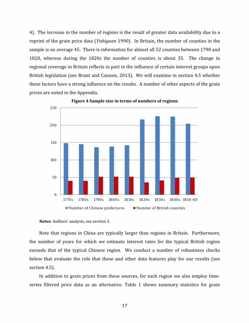
4). The increase in the number of regions is the result of greater data availability due to a

reprint of the grain price data (Yishiguan 1990). In Britain, the number of counties in the

sample is on average 45. There is information for almost all 52 counties between 1790 and

1820, whereas during the 1820s the number of counties is about 35. The change in

regional coverage in Britain reflects in part in the influence of certain interest groups upon

British legislation (see Brunt and Cannon, 2013). We will examine in section 4.5 whether

these factors have a strong influence on the results. A number of other aspects of the grain

prices are noted in the Appendix.

Figure 4 Sample size in terms of numbers of regions

Note that regions in China are typically larger than regions in Britain. Furthermore,

the number of years for which we estimate interest rates for the typical British region

exceeds that of the typical Chinese region. We conduct a number of robustness checks

below that evaluate the role that these and other data features play for our results (see

section 4.5).

In addition to grain prices from these sources, for each region we also employ time-

series filtered price data as an alternative. Table 1 shows summary statistics for grain

0

50

100

150

200

250

1770s 1780s 1790s 1800s 1810s 1820s 1830s 1840s 1850-60

Number of Chinese prefectures Number of British counties

Notes: Authors’ analysis, see section 3.

18

prices filtered with the Butterworth (1930) band pass filter. Furthermore, storage costs

might change over time in relationship to climatic conditions. For example, clean and dry

grain can be stored for longer periods, whereas very wet conditions are conducive to mold

unless the grain is well protected against moisture. We have collected annual information

on climatic conditions at the regional level to take into account how weather variations

might affect storage costs.

The historical data on Chinese weather comes from the State Meteorological Society

(1981). The source contains historical weather data in the form of contour maps based on

the climate in autumn at 120 weather stations throughout China over the years of analysis.

Based on these contour maps and the location of each prefecture we categorize the climate

in a given prefecture for a given year as ranging from 1 (a lot of rainfall leading to very wet

conditions) to 5 (little rainfall leading to very dry conditions), with 3 being the normal level

of rainfall. Reference to a “normal” regional climate implies that the average climate is

close to level 3 (with an average of 2.92 for the prefectures in our sample). Figure 5

summarizes this data on climate over time across the Chinese prefectures.

We construct data on the climate in Britain with the precipitation reconstructions

from Pauling et al. (2006) according to the definitions of wetness in the Chinese data.1 As a

consequence, the mean (i.e. normal) climate level is, as in the Chinese data, roughly 3.

Figure 6 shows the variability of weather in Britain. Also the standard deviation of rainfall

in a given year across regions is shown in Figures 5 and 6. On average the standard

deviation is higher in China than in Britain, no doubt in part because of China’s relatively

large size. For a given region in China or Britain, weather variability over the sample

period is comparable, with a standard deviation of 0.98 in China and of 1.16 in Britain.

1 We use annual rainfall for Britain to avoid introducing a time-varying difference between the British and Chinese weather data given the distinction between lunar and solar months.

19

Figure 5 Climate in China: Annual wetness across regions, 1770 - 1860

Figure 6 Climate in Britain: Annual rainfall across regions, 1770 to 1860

To examine how interregional trade and cropping patterns can affect grain price

behavior between harvests, the empirical analysis below also employs indicator variables

for waterway location and areas where multiple crops can be harvested in a given year. We

include the major waterways in the analysis (Watson 1972, Paget-Tomlinson 1993): the

0

0.5

1

1.5

2

2.5

3

3.5

4

4.5

1770

1773

1776

1779

1782

1785

1788

1792

1795

1798

1801

1804

1808

1811

1814

1817

1820

1823

1826

1829

1832

1835

1838

1841

1844

1847

1850

1853

1856

1859

Mean wetness Standard deviation of wetness

0

1

2

3

4

5

6

1770

1773

1776

1779

1782

1785

1788

1791

1794

1797

1800

1803

180

618

09

1812

1815

1818

1821

1824

1827

1830

1833

1836

1839

1842

1845

1848

1851

1854

1857

1860

Mean rainfall Standard deviation of rainfall

Notes: Data from State Meteorological Society (1981)

Notes: Data from Pauling, Luterbacher, Casty, and Wanner (2006)

20

Yangzi and the Pearl river in China, and the Thames, Trent, Severn, and Lea in Britain;

among the canals we focus on the Grand Canal in China and the Bridgewater Canal in

Britain. We also take account of coastal location; for China given its size this is done

separately for the North and the South, as well as for the Yangzi delta.

In terms of differences in cropping patterns, the most important factor is that in parts

of Southern China, rice can be harvested twice in a given year (Chuan and Kraus 1975,

LeClerc 1927). We account for this by including an indicator variable for these regions.

4. Empirical results

4.1 Grain Price Changes and Interest Rates in Britain and China

We begin by showing evidence on the average percentage grain price changes, 𝜋𝜋𝑖𝑖𝑖𝑖, also

referred to carry costs of grain, before turning to the interest rates. The mean monthly

price change for British counties based on the log wheat price series is about 0.85%, or

10.2% per year (Table 2). In contrast, across all Chinese regions and based on all grains,

the mean is about 13.7% annually. Results based on filtered price series are shown in the

lower part of Table 2. These figures are generally lower than for those based on the

unfiltered time series, consistent with the idea that time series filtering removes stochastic

trends. According to the filtered series, British price changes average around 8.2% per

year while Chinese price changes are around 9.6%. Additional analysis across different

types of grain for China shows that the differences across grains are small. This is plausible

because storage costs and other factors are unlikely to vary greatly across grains.1

1 The analysis by grain also provides evidence on the influence of the frequency of non-zero price changes (last column, Table 1).

21

Having estimated the average monthly price changes over the growing season, the

following section is concerned with assessing the part in these price changes that is due to

non-interest rate factors, especially physical storage costs. To do so we perform a three-

stage adjustment to purge the influence of climate, water access and cropping pattern from

the average annual price changes.

Our proxy for climatic conditions is 𝑟𝑟𝑟𝑟𝑖𝑖𝑟𝑟𝑖𝑖𝑖𝑖, defined as the rainfall level in region i and

year t measured in five bins.1 We perform OLS regressions separately for each larger

geographic area of the price change 𝜋𝜋𝑖𝑖𝑖𝑖 on 𝑟𝑟𝑟𝑟𝑖𝑖𝑟𝑟𝑖𝑖𝑖𝑖 to obtain the average price change for

each rain level.2 The level of 𝑟𝑟𝑟𝑟𝑖𝑖𝑟𝑟𝑖𝑖𝑖𝑖 with the lowest average price change is assumed to be

the climate with the lowest storage costs. We adjust the price change of region i and year t

1 Our climate data varies from 1 (highest level of rain) over 3 (normal levels) to 5 (lowest level of rain); see the Appendix for details. 2 Larger areas are defined as the provinces of China. We assume that all British counties belong to the same larger geographic area.

Table 2. Average monthly grain price changes, 1770 to 1860

Monthly rate Annualized n Mean (%) Std. dev. (%) Britain Wheat 4,074 0.854 2.577 10.248 China All grains 15,152 1.144 2.446 13.732

China Wheat 4,930 1.124 2.577 13.488

Millet 3,973 1.020 2.598 12.242

Rice 1st quality 5,135 1.071 1.978 12.854

Rice 2nd quality 5,384 1.074 2.133 12.883

Bandpass filtered Britain Wheat 4,102 0.684 2.239 8.209 China All grains 13,403 0.801 2.172 9.612

China Wheat 4,221 0.774 1.886 9.284

Millet 3,314 0.684 2.000 8.210

Rice 1st quality 4,366 0.761 2.048 9.131

Rice 2nd quality 4,794 0.781 2.054 9.376

Notes: Average monthly grain price changes during storage months. Weighted by the fraction of month-to-month prices changes that are non-zero (see Table 1). Annual rates are computed as 12 times the monthly rate.

22

using the difference of the OLS estimates for the lowest-storage cost climate and the actual

climate in that region and year. The resulting price changes are those that would have

prevailed had the climate always been such that storage costs were minimal for all regions

and years. This adjustment ensures that any difference in the price changes in China and

Britain is not driven by climatic effects. Table 3 shows the results in column 2.

Our results confirm that climate has a substantial influence on storage costs and

within-harvest year grain price changes. Comparing the previous figures with the climate-

adjusted figures shows that in the case of the unfiltered series, the climate-adjusted figures

are around five percentage points lower than the figures that are gross of climate-induced

storage costs (columns 1 and 2, Table 3). There is also a substantial difference between

climate-adjusted and unadjusted price changes using filtered price series (Panel B).

At the same time, adjusting for climate does not overturn our earlier finding that price

changes tend to be lower in Britain than in China. This is because the extent to which

variation in climate affects storage costs does not differ very much between China and

Britain. It is around 4 to 5 percentage points for price changes based on unfiltered series

and 2 to 3 percentage points for price changes based on bandpass filtered series.

We now turn to adjusting for the impact of inter-regional trade. To do so we employ

regional information on access to water transport, which was the low-cost mode of

transport for grain at the time.1 The climate-adjusted price changes are projected on

indicator variables for river, canal, or coastal water access using an OLS regression. Based

on the resulting coefficients we compute price changes standardized for the lowest-storage

cost climate and no access to water transport. The average of these figures is shown in

Table 3, column 3. Comparing columns 2 and 3 we see that inter-regional trade does not

have a major influence on intra-harvest year price changes once climate variation has been

taken into account.

1 Information on trade volumes within China becomes only available towards the end of the 19th century (see, e.g., Keller, Santiago, and Shiue 2017 for an analysis).

23

Table 3. Grain interest rates: the influence of weather, trade, and harvest patterns

Price Change Interest rate Interest rate broad

Adjustments

None (1)

Climate (2)

Climate & Waterway

(3)

Climate & Waterway &

Harvest Patterns (4)

Climate & Waterway &

Harvest Patterns

(5)

Panel A. Unfiltered data

Britain Mean in % 10.248 (30.924)

5.271 (30.804)

5.348 (30.795)

5.348 (30.795)

5.348 (30.795)

n 4,074 4,074 4,074 4,074 4,074

China Mean in % 13.732 (29.350)

9.374 (29.040)

9.440 (29.088)

9.200 (29.077)

6.258 (24.544)

n 15,152 15,152 15,152 15,152 18,586

Panel B. Band-pass filtered data

Britain Mean in % 8.209 (26.868)

4.891 (26.808)

5.415 (26.772)

5.415 (26.772)

3.204 (15.684)

n 4,102 4,102 4,102 4,102 4,115

China Mean in % 9.612 (26.064)

7.616 (25.800)

7.482 (25.934)

7.501 (25.814)

4.023 (15.946)

n 13,403 13,403 13,403 13,403 19,736 Notes: Shown are statistics for average monthly grain price changes with various adjustments in columns (1) to (3); statistics for the preferred grain interest rates are shown in column (4). “Interest rate broad” is calculated using grain price gradient in all months that typically exhibit price increases. Standard deviation given in parentheses.

24

Finally, we adjust for differences in harvest patterns. This might matter because

rice was typically harvested twice each year in Fujian, Guangdong, and Guangxi

provinces. Defining an indicator variable that is equal to one for regions in which

such double cropping was possible, we perform a regression adjustment analogous

to that for climate and inter-regional trade. Column 4 in Table 3 gives the average

price changes that adjust in addition to low-cost climate and no water access would

have prevailed in the absence of double cropping. We see that the influence of

harvest patterns is quite small, no doubt in part because it affects only a subset of

regions.1

These three adjustments of the price changes πit yield our interest rates rit,

using the storage cost approach. Among the factors affecting storage costs �̃�𝑐𝑖𝑖𝑖𝑖we

find climate to be the most important. The average interest rate for Britain is about

5.3% and for China it is about 9.2%. Employing time-series filtered grain price

series the averages are 5.4% and 7.5%, respectively. Thus, there is evidence that

interest rates in China were substantially higher than in Britain over the sample

period 1770 to 1860, by about two to four percentage points.2 At the same time, the

difference is not as large as one might expect given the existing literature.

The reported standard deviations in Table 3 show that the interest rates exhibit

a relatively large amount of variability. Interest rates can be high when shocks lead

to sharp price increases, and they can be low and even negative in particular years

as well. With relatively few observations it might be difficult to estimate the typical

level of interest rate. With this in mind, Figure 7 shows the smoothed interest rate

average for Britain and China between 1770 and 1860. The average British rate is

consistently between 5 and 6%, while the average Chinese rate fluctuates between

1 Interactions between climate, water access, and cropping patterns do not have a major influence on our results. Note that by relying on nominal price changes, our analysis estimates nominal, not real interest rate estimates. Studies of early capital market development using bank interest rates typically focus on nominal interest rates as well because there is often little systematic data to construct local price indices (other than grain price data). We have also considered the possible influence of double-cropping of wheat and barley, which is noted by Perkins (1969), finding its role to be negligible for our main results. 2 Furthermore, there is a substantial difference with or without adjusting for climate, trade, and cropping patterns.

25

almost 10% around 1795 to just under 8% around the year 1835. We discuss

regional variation in China, in particular the Yangzi Delta, in section 4.3 below.

Figure 7 Interest rates over time, 1770 to 1860

The impact of employing all months with a gradient greater than 0 in the

interest rate calculation (as opposed to the 5% threshold in column 4) is shown in

column 5 of Table 3. The interest rate averages tend to fall, which is not surprising

because more months without grain storage are included in the analysis. At the

same time, on average British rates are still lower than Chinese rates by close to one

percentage point (see column 5). Thus, the finding of relatively low British rates is

robust to taking the broad approach of computing storage price gradients with all

months that show positive price changes.

We now turn to our second measure of capital market performance, the

regional integration of markets.

4.2 The integration of capital markets

0

0.02

0.04

0.06

0.08

0.1

0.12

Ave

rage

an

nu

al in

tere

st r

ate

Britain China

Notes: Data from State Meteorological Society (1981)

26

This section compares the capital market performance in Britain and China in

terms of bilateral correlations of regional interest rates over time. A high level of

correlation indicates strong forces that integrate capital markets across the two

regions. The degree of capital market integration typically falls in geographic

distance. For one, in historical contexts capital market participants often had to

meet in person to trade, and in the presence of costs of moving in geographic space

there will be fewer such meetings. Even when trades are made indirectly through

middlemen, geography is often an important barrier. Information about investment

projects, trust, and enforcement for example will tend to be more difficult as

geographic distance increases. We therefore report bilateral correlations for

different distances, from 0-100 kilometers to 500-600 kilometers.1 Let 𝛾𝛾𝑑𝑑𝑐𝑐 denote

the average bilateral interest rate correlation within the dth distance bins in country

c, with d = 1,…,6 and c = B or C, for Britain and China, respectively.

Figure 8 shows the average bilateral correlation by distance bin based on the

interest rates of all regions in each country over all years from 1770 to 1860. For

each country, two curves are shown, one for capital market integration based on

unfiltered and the other based on time-series filtered grain price data. The main

takeaway is that the integration of British capital markets was considerably higher

than that of China’s capital markets. Looking at correlations based on unfiltered

interest rates (solid lines), for distances below 100 kilometers 𝛾𝛾1𝐵𝐵 = 0.8 for Britain

while 𝛾𝛾1𝐶𝐶 is less than 0.6 in China. Even more striking is the difference in capital

market integration at higher distances. While in China the correlation falls from

about 0.6 to around 0.1 as distance increases, in Britain the correlation falls only

from 0.8 to 0.7 for the same increase in distance.

It is worth noting that although correlations for filtered interest rates are

generally somewhat lower, the comparison between Britain and China based on the

filtered interest rates yields very similar patterns. At short distances, interest rate

correlations in Britain are higher than in China: 0.7 compared to 0.4, respectively.

1 We cap the analysis at 600 kilometers because the maximum distance between any two British county capitals in our sample is 638 kilometers.

27

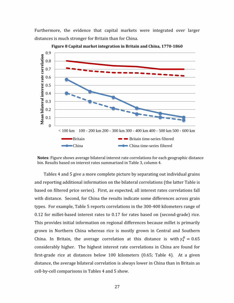
Furthermore, the evidence that capital markets were integrated over larger

distances is much stronger for Britain than for China.

Figure 8 Capital market integration in Britain and China, 1770-1860

Tables 4 and 5 give a more complete picture by separating out individual grains

and reporting additional information on the bilateral correlations (the latter Table is

based on filtered price series). First, as expected, all interest rates correlations fall

with distance. Second, for China the results indicate some differences across grain

types. For example, Table 5 reports correlations in the 300-400 kilometers range of

0.12 for millet-based interest rates to 0.17 for rates based on (second-grade) rice.

This provides initial information on regional differences because millet is primarily

grown in Northern China whereas rice is mostly grown in Central and Southern

China. In Britain, the average correlation at this distance is with 𝛾𝛾4𝐵𝐵 = 0.65

considerably higher. The highest interest rate correlations in China are found for

first-grade rice at distances below 100 kilometers (0.65; Table 4). At a given

distance, the average bilateral correlation is always lower in China than in Britain as

cell-by-cell comparisons in Tables 4 and 5 show.

0

0.1

0.2

0.3

0.4

0.5

0.6

0.7

0.8

0.9

< 100 km 100 - 200 km 200 - 300 km 300 - 400 km 400 - 500 km 500 - 600 km

Mea

n bi

late

ral i

nter

est r

ate

corr

elat

ion

Britain Britain time-series filteredChina China time-series filtered

Notes: Figure shows average bilateral interest rate correlations for each geographic distance bin. Results based on interest rates summarized in Table 3, column 4.

28

Table 4. Capital market integration in comparison Based on log grain price data

Britain China Wheat Wheat Rice 1st quality Rice 2nd quality Millet 0-100km 0.80

(0.16) [n = 350]

0.53 (0.38)

[n = 186]

0.65 (1.18)

[n=196]

0.56 (0.62)

[n=202]

0.54 (0.36)

[n=152] 100-200km 0.77

(0.16) [n = 788]

0.41 (0.55)

[n = 566]

0.45 (1.37)

[n=602]

0.40 (0.69)

[n=628]

0.44 (0.38)

[n=484] 200-300km 0.74

(0.17) [n = 720]

0.30 (0.43)

[n=730]

0.39 (1.43)

[n=758]

0.36 (0.72)

[n=840]

0.35 (0.45)

[n=616] 300-400km 0.73

(0.18) [n = 476]

0.21 (0.39)

[n=786]

0.20 (0.80)

[n=802]

0.22 (1.01)

[n=902]

0.25 (0.43)

[n=684] 400-500km 0.70

(0.18) [n = 246]

0.11 (0.49)

[n = 886]

0.20 (2.07)

[n=908]

0.14 (0.88)

[n=1,108]

0.17 (0.38)

[n=568] 500-600km 0.70

(0.19) [n = 64]

0.07 (0.48)

[n=1,002]

0.11 (2.04)

[n=1,018]

0.11 (1.22]

(n=1,184)

0.12 (0.27)

[n=548] Notes: Entries are average correlations over period 1770 to 1860. Interest rates as underlying Table 3, Panel A, column 4. Standard deviations in parentheses.

29

Table 5. Capital market integration in comparison – based on time-series filtered series

Britain China Wheat Wheat Rice 1st quality Rice 2nd quality Millet 0-100km 0.71

(0.17) [n = 350]

0.35 (0.28)

[n = 138]

0.44 (0.50)

[n=166]

0.51 (0.46)

[n=158]

0.29 (0.34)

[n=134] 100-200km 0.68

(0.18) [n = 788]

0.26 (0.30)

[n = 424]

0.34 (0.56)

[n=500]

0.35 (0.54)

[n=494]

0.24 (0.35)

[n=390] 200-300km 0.66

(0.17) [n = 720]

0.21 (0.33)

[n=556]

0.23 (0.62)

[n=620]

0.25 (0.58)

[n=612]

0.16 (0.35)

[n=482] 300-400km 0.65

(0.16) [n = 476]

0.13 (0.31)

[n=560]

0.16 (0.73)

[n=628]

0.17 (0.56)

[n=660]

0.12 (0.34)

[n=514] 400-500km 0.63

(0.19) [n = 246]

0.10 (0.34)

[n = 630]

0.15 (0.78)

[n=658]

0.10 (0.55)

[n=804]

0.07 (0.33)

[n=398] 500-600km 0.62

(0.23) [n = 64]

0.07 (0.34)

[n=706]

0.07 (0.75)

[n=682]

0.08 (0.62]

(n=802)

0.03 (0.29)

[n=374] Notes: Entries are average correlations over period 1770 to 1860. Interest rates as underlying Table 3, Panel B, column 4. Standard deviations in parentheses.

30

Figure 9A Bilateral interest rate correlations versus distance, 1770-1860

Figure 9B All British bilateral interest rate correlations, 1770 to 1860

Smoothed Line for China

Notes: All bilateral interest rate correlations based on filtered grain prices.

31

An even more complete picture of capital market integration emerges by

comparing the full distribution of bilateral interest rate correlations in China and in

Britain. In Figure 9A we show those distributions plotted against bilateral

geographic distance. The hollow circles mark bilateral interest rate correlations in

Britain, and the plus-signs mark observations for China. The British circles fill out

the upper part of the figure, indicating higher levels of capital market integration for

a given distance. The figure also shows the smoothed mean correlation for China

(dashed line). Figure 9B shows the same figure with the Chinese markers hidden. It

makes clearer that the observations for Britain are positioned almost entirely above

the China smoothed line. The evidence in Figure 9A and Figure 9B strongly

indicates that the degree of integration of British capital markets exceeded the

integration in Chinese capital markets over the sample period 1770-1860.

The analysis has shown that capital market integration in Britain was higher

than in China. However, with China having several times the size of Britain, it is

important to ask how the most developed areas of China compared to Britain. The

following section focuses on the Yangzi Delta, the most advanced area within China

from an economic development viewpoint.

4.3 Britain versus the Yangzi Delta

Pomeranz (2000) emphasizes that a comparison of other parts of the world

with China should account for the heterogeneity within China, given her large size.

To be specific, we should not compare capital markets in the relatively less

developed regions of China’s vast territory with capital markets in Lancashire,

where the world’s first factory-based textile industry emerged.

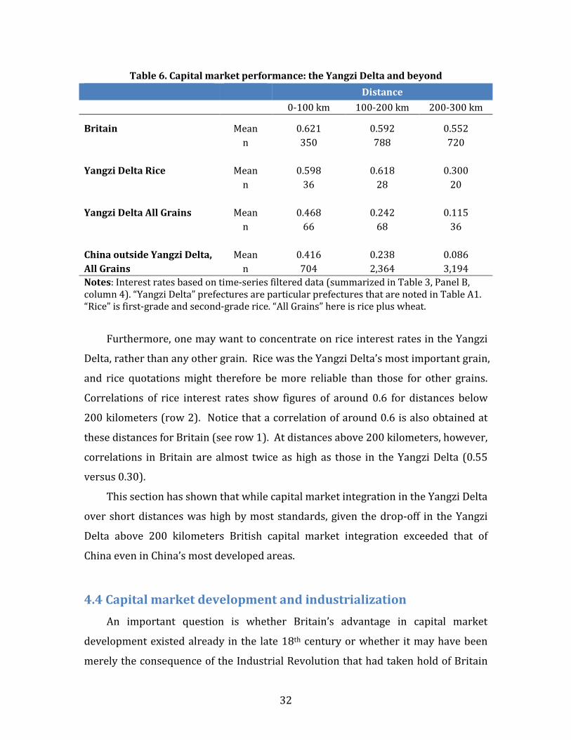
We show results that distinguish less from more developed regions with in

China in Table 6. The average interest rate correlation in China’s Yangzi Delta is

0.47 at distances below 100 kilometers, higher than outside of the Delta (0.42, last

row). There is also evidence for relatively high capital market integration in the

Delta at distances above 100 kilometers (column 2 and 3). Our results are in line

with other evidence that the Yangzi Delta was relatively highly developed.

32

Furthermore, one may want to concentrate on rice interest rates in the Yangzi

Delta, rather than any other grain. Rice was the Yangzi Delta’s most important grain,

and rice quotations might therefore be more reliable than those for other grains.

Correlations of rice interest rates show figures of around 0.6 for distances below

200 kilometers (row 2). Notice that a correlation of around 0.6 is also obtained at

these distances for Britain (see row 1). At distances above 200 kilometers, however,

correlations in Britain are almost twice as high as those in the Yangzi Delta (0.55

versus 0.30).

This section has shown that while capital market integration in the Yangzi Delta

over short distances was high by most standards, given the drop-off in the Yangzi

Delta above 200 kilometers British capital market integration exceeded that of

China even in China’s most developed areas.

4.4 Capital market development and industrialization An important question is whether Britain’s advantage in capital market

development existed already in the late 18th century or whether it may have been

merely the consequence of the Industrial Revolution that had taken hold of Britain

Table 6. Capital market performance: the Yangzi Delta and beyond Distance

0-100 km 100-200 km 200-300 km Britain Mean 0.621 0.592 0.552

n 350 788 720

Yangzi Delta Rice Mean 0.598 0.618 0.300

n 36 28 20

Yangzi Delta All Grains Mean 0.468 0.242 0.115

n 66 68 36

China outside Yangzi Delta, Mean 0.416 0.238 0.086 All Grains n 704 2,364 3,194 Notes: Interest rates based on time-series filtered data (summarized in Table 3, Panel B, column 4). “Yangzi Delta” prefectures are particular prefectures that are noted in Table A1. “Rice” is first-grade and second-grade rice. “All Grains” here is rice plus wheat.

33

in the late 18th century. Figure 10 shows bilateral interest rate correlations in China

and Britain for the years 1770 to 1794.

Comparing it with Figure 9, which shows bilateral interest rate correlations for

the entire sample period (1770 to 1860), it is striking finding how large Britain’s

advantage over China already was during the period 1770 to 1794. Given the stark

difference during the period 1770 to 1794, as shown in Figure 10, a large gap must

have existed well before the onset of Britain’s own higher rate of economic growth

with the industrial revolution. If we were to follow convention and use 1770 as the

start date of British industrialization, our findings are consistent with capital market

development being an important factor in explaining why Britain industrialized first.

Whether Britain’s early industrialization was caused by its relatively high capital

market development remains an open question; however, our comparison with

China has established that this is a pressing question.

Figure 10 Bilateral interest rate correlations, 1770-1794

-1-.

50

.51

0 2 4 6Dista nce (in 100 kilom et ers)

Ch ina Britain Ch ina sm ooth ed

Notes: All bilateral interest rate correlations based on filtered grain prices, years 1770 to 1794.

34

We now turn to several other potentially important factors in this analysis.

4.5 Further Discussions

4.5.1 Region size and the role of spatial aggregation

Chinese prefectures are on average roughly twice as large as British counties.

To see the implications of this we have paired up the 52 British counties into 26

regions of roughly similar size. Taking the same steps as before for these larger

British regions, we compare bilateral interest rate correlations resulting from this

set of 26 regions with the results from before based on the 52 counties. In Table 7,

the latter are denoted by “Baseline” (left two columns) while the former are denoted

by “Aggregated”.

Table 7. Spatial Aggregation and capital market integration Baseline Aggregated Unfiltered Filtered Unfiltered Filtered

0-100 km 0.80 (0.16)

[n = 350]

0.71 (0.17)

[n = 350]

0.85 (0.10)

[n = 42]

0.81 (0.11)

[n = 42] 100-200km 0.77

(0.16) [n = 788]

0.68 (0.18)

[n = 788]

0.82 (0.13)

[n = 162]

0.74 (0.13)

[n = 162] 200-300km 0.74

(0.17) [n = 720]

0.66 (0.17)

[n = 720]

0.81 (0.12)

[n = 170]

0.71 (0.11)

[n = 170] 300-400km 0.73

(0.18) [n = 476]

0.65 (0.16)

[n = 476]

0.80 (0.12)

[n = 132]

0.70 (0.11)

[n = 132] 400-500km 0.70

(0.18) [n = 246]

0.63 (0.19)

[n = 246]

0.78 (0.13)

[n = 74]

0.69 (0.11)

[n = 74] 500-600km 0.70

(0.19) [n = 64]

0.62 (0.23)

[n = 64]

0.79 (0.19)

[n = 20]

0.67 (0.15)

[n = 20] Notes: All results are for Britain. Shown in the Baseline columns are results for 52 counties. In the Aggregated columns, the 52 counties are aggregated to 26 regions that on average closely resemble the size of a Chinese prefecture.

35

We see that aggregation increases the correlations somewhat. Furthermore, it

does so for all geographic distance categories. This implies that our findings are not

driven by the relatively small size of the regions in Britain. On the contrary, if

anything the difference in region size has put Britain at a disadvantage relative to

China.

4.5.2 Storage months

We are interested in the effect of adding relatively flat parts of the within-

harvest year price curve on the interest rate correlations. The dashed line in Figure

11 depicts the average correlations using this broader definition of storage months,

which is compared with the baseline results (solid in Figure 11). Generally, the

broader definition of storage months leads to a lower degree of capital market

integration. However, irrespective of whether we adopt the preferred or the

broader definition of storage months, there is evidence that the integration of

capital markets in Britain was higher than in China.

Figure 11 Capital market integration comparison and storage months

-0.1

0

0.1

0.2

0.3

0.4

0.5

0.6

0.7

0.8

< 100 100 - 200 200 - 300 300 - 400 400 - 500

Mea

n in

tere

st r

ate

corr

elat

ion

Distance (kilometers)

Britain China

Britain broad storage month def. China broad storage month def.

36

4.5.3 Convenience yields, volatility, and inventories

Since convenience yields are unobserved we employ price information to

identify periods of high inventory, exploiting the well-established inverse

relationship between inventories and convenience yields. Table 8 provides results

for three alternative criteria that give periods of low convenience yields, based on

current and past price levels as well as price volatility (see the Notes to Table 8).

These criteria are applied in the same way to both Chinese and British regions.

Table 8 reports average interest rate correlations for the subsamples that

satisfy the particular low convenience yield criteria. Across the board, we see that

the analysis confirms a higher level of capital market integration in Britain than in

China. It is thus unlikely that variation in convenience yields over time and across

regions is important for explaining our findings.

Table 8. Convenience yields, storage, and capital market integration

Less than 10% above price trend

No consecutive price increases Low volatility

Britain China Britain China Britain China

0 to 200 km 0.776 (1,138)

0.438 (748)

0.782 (1,128)

0.441 (738)

0.732 (1,128)

0.388 (712)

200 to 400 km 0.734 (1,196)

0.252 (1,482)

0.748 (1,176)

0.264 (1,412)

0.677 (1,174)

0.193 (1,320)

400 to 600 km 0.722 (310)

0.124 (1,780)

0.727 (298)

0.145 (1,626)

0.631 (298)

0.086 (1,384)

Notes: Entries give average bilateral interest rate correlation; number of observations given in parentheses. Results for three different subsamples during which convenience yields are expected to be low are shown. Less than 10% above price trend: Compute 5 period moving average trend based on annual average grain prices; identify all years in which actual price is less than 10% above this moving average trend. No consecutive price increases: Construct indicator variable equal to 1 if region has seen three or more consecutive price increases leading up to year t; results based on data for which indicator is 0. Low volatility: For year t and month m, compute price volatility as the standard deviation of prices in years t-1, t, and t+1. Take the average of these twelve month-specific standard deviations as the volatility of year t. Analysis is based on the lower 75 percent of observations in terms of volatility.

4.5.4 Sample composition and zero grain price changes

There are on average more than 170 Chinese prefectures in the sample for a

given year, with just under 150 prefectures before 1820 and around 215 thereafter.

Notes: Shown are average bilateral interest rate correlations for a relatively narrow (solid) versus a relatively broad (dashed) definition of months during which there was grain storage.

37

In Britain, the number of counties in the sample is on average 45. There is

information for almost all 52 counties between 1790 and 1820, whereas during the

1820s the number of counties is about 35.

Because such changes might affect the results we have conducted the analysis

of capital market integration for the period before and after 1820 separately (see

Table 9).1 As it turns out, even though the change in the number of regions from

one period to the other is at times substantial, we do not see evidence that this

systematically affects the results for Britain. For China, there is some evidence for

lower levels of integration after the year 1820 for short distances. This finding,

however, is to some extent reversed at distances between 500 and 600 kilometers,

leaving no clear overall pattern.

Table 9. The role of sample composition: results before and after 1820 Britain China Before 1820 After 1820 Before 1820 After 1820 0-100 km 0.73

(0.20) [n = 350]

0.72 (0.23)

[n = 314]

0.38 (0.32)

[n = 116]

0.29 (0.32)

[n = 108] 100-200km 0.69

(0.22) [n = 788]

0.71 (0.23)

[n = 724]

0.28 (0.40)

[n = 380]

0.23 (0.30)

[n = 274] 200-300km 0.66

(0.21) [n = 720]

0.69 (0.26)

[n = 660]

0.21 (0.42)

[n = 472]

0.22 (0.35)

[n = 380] 300-400km 0.66

(0.22) [n = 476]

0.68 (0.24)

[n = 430]

0.15 (0.36)

[n = 474]

0.14 (0.36)

[n = 288] 400-500km 0.64

(0.28) [n = 246]

0.66 (0.21)

[n = 216]

0.10 (0.33)

[n = 478]

0.09 (0.43)

[n = 276] 500-600km 0.56

(0.42) [n = 64]

0.67 (0.24)

[n = 58]

0.06 (0.34)

[n = 530]

0.09 (0.39)

[n = 278] Notes: Results for average of bilateral correlations of interest rates based on filtered wheat prices. Standard deviation in parentheses.

We have also examined the role of unchanged month-to-month prices for our

results. As shown in Table 1, generally British prices exhibit more non-zero price

changes than the price series for China. This raises the question whether the higher

1 This also sheds light on the role of the British Corn Laws (1815-46) for our results.

38

share of non-zero price changes explains our findings of relative capital market

development.

To address this issue we have exploited differences in the share of zero price

changes across the four grains in China. For example, there are about 50% fewer

zero price changes for first quality rice than for wheat in the data (Table 1, last

column). We relate these differences across grain to the average bilateral interest

rate correlations by grain given in Tables 4 (unfiltered data) and 5 (filtered data). It

turns out that there is no significant relationship between the share of zero price

changes by grain and capital market integration by grain using filtered price series.1

For our measures of capital market integration based on unfiltered prices, there is a

significant positive relationship, however it cannot explain our finding of relative

capital market integration. Specifically, if Chinese series had the same share of zero

price changes as the British, the average bilateral correlation for China would be

0.48, compared to 0.74 for Britain.2 Thus, even if we were to believe that there is a

relationship between non-zero price changes and measured market integration, the

effect would not be big enough to explain our findings.

4.5.5 Capital market integration and time series length

Another issue may be that we calculate the interest rate correlations based on

different numbers of annual observations. For some pairs there are interest rates

over the entire sample period 1770 to 1860, while for others only for a subset of

years. Any difference between China and Britain in this respect might matter if the

strength of interest rate correlation is related to time series length. We analyze this

issue by examining correlations for all region pairs with a fixed number of years,

namely 50 to 70 years. See Table 10 for the results.

We see that time series length plays some role for the results. Generally, we

find little difference in using all pairs versus the pairs with 50 to 70 years of data for 1 An OLS regression of the average bilateral correlation across all 6 distance bins from Table 5 on the share of non-zero price changes yields a slope coefficient of 0.23 and a s.e. estimate of 0.35. 2 The OLS regression of the average bilateral correlation across all 6 distance (y) from Table 4 on non-zero price changes (x) gives 𝑦𝑦� = 0.16 + 0.32𝑥𝑥; employing the x value of Britain (which is 0.994) gives 0.16 + 0.32 × 0.994 = 0.48.

39

Britain (Table 10, columns 1 and 2). For China, the focus on pairs with 50 to 70

years of data leads to higher average correlations (compare columns 3 and 4). As a

consequence, controlling for time series length moves China’s market integration

closer to the levels observed in Britain. Nevertheless, at distances above 300

kilometers, however, correlations for British regions are typically still more than

twice as high as those in China.

Table 10. Capital market integration and time series length Britain China All data 50 < x < 70 All data 50 < x < 70 0-100 km 0.71

(0.17) [n = 350]

0.68 (0.18)

[n = 92]

0.51 (0.46)

[n = 158]

0.61 (0.50)

[n = 56] 100-200km 0.68

(0.18) [n = 788]

0.67 (0.18)

[n = 222]

0.35 (0.54)

[n = 494]

0.46 (0.61)

[n = 164] 200-300km 0.66

(0.17) [n = 720]

0.67 (0.16)

[n = 224]

0.25 (0.58)

[n = 612]

0.36 (0.49)

[n = 118] 300-400km 0.65

(0.16) [n = 476]

0.65 (0.13)

[n = 136]

0.17 (0.56)

[n = 660]

0.33 (0.23)

[n = 66] 400-500km 0.63

(0.19) [n = 246]

0.65 (0.14)

[n = 80]

0.10 (0.55)

[n = 804]

0.22 (0.29)

[n = 48] 500-600km 0.62

(0.23) [n = 64]

0.66 (0.12)

[n = 28]

0.08 (0.62)

[n = 802]

0.19 (0.55)

[n = 108] Notes: Results for average of bilateral correlations of interest rates based on filtered wheat prices for Britain and based on filtered second-grade rice prices for China. Results for columns “50 < x < 70” are for pairs of regions with 50 to 70 years of data in the period 1770 to 1860. Standard deviation in parentheses; number of observations in brackets.

Summarizing the analyses in sections 4.5.1 to 4.5.5, we do not find strong

patterns except for time series length, which favors Britain, and region size, which

favors China. Overall, our finding of higher levels of capital market integration in

Britain than in China is robust.

40

5. Conclusions We have shown that Britain had an advantage over China in terms of the

development of its capital market, which manifested itself both in lower interest

rates and in higher capital market integration. Comparable interest rates in China

were on the order of two to four percentage points higher, and market integration

was substantially lower in China than in Britain, even in China’s most developed

areas once we move outside relatively short distances.

Our finding of lower integration of capital markets means that capital was not

flowing to the location of efficient use in China to the extent it did in Britain. The

differential in interest rates levels, by contrast, was not very large. This suggests

that is was not capital scarcity that mattered so much as the appropriate allocation

of existing capital. It is useful to compare this result with commodity market

integration. During the 18th century, Britain was slightly ahead, but not by such large

margins (Shiue and Keller 2007). In addition, European commodity integration

dramatically improved shortly after the 19th century, whereas there does not appear

to be sharp jumps in capital market integration. This suggests that not only were

British capital markets much more integrated than they were in China, and

therefore working much better, but the lack of large improvements in capital market

integration suggests that these markets were already operating fairly well in Europe.

It may also be an indication that improvements in capital markets take longer to

establish and operationalize effectively.

Further research is needed to determine what explains the lower regional

capital market integration in China compared to Britain. Some accounts suggest that

the wealthy in China in the 18th and 19th centuries did not conduct much capital

accumulation. The salt merchants of Yangzhou, for example, the wealthiest

merchants of this time, saw their wealth dissipate in a few generations (Ho 1954).

Investments flowed into political connections or for the grooming of sons to enter

the civil service examinations and a career in officialdom, rather than towards the

preservation or expansion of family wealth.

41

Another possible explanation is that the Chinese empire, up until the Taiping

Rebellion of the 19th century, was a balanced budget state, meaning that it never

borrowed, and therefore had no experience with bonds and other financial

instruments. The first stock market in China was introduced by foreigners

(Goetzmann, Ukhov, and Zhu 2007).1 In England, by contrast, the state as well as

state-backed ventures such as the East India Company created opportunities and

investment strategies with financial innovations such as limited liability joint stock

companies. There is probably some truth to this state finance hypothesis, although

very little is known at this point on its quantitative importance.

Our finding of low capital market integration over long distances in China is

consistent with the hypothesis that borrowing and lending is segmented

geographically because of the importance of local lineages (common descent

groups). Along these lines, China’s relatively low capital market integration would

reflect the delayed transition in China from kinship-based financial transactions to

impersonal transactions, especially those involving banks.

Regardless of the reasons, the large gap in capital market integration that

results matters to economic efficiency in ways that are distinct from commodity

markets. Whereas commodity markets match buyers and sellers, as in an

endowment economy model in which lychees and apples fall from trees and are in

turn traded for other consumption goods, capital markets, in contrast, channel

resources from individuals willing to postpone consumption to others with

productivity-enhancing projects that pay off in the future. The finding of low

regional capital market integration provides evidence that the process of matching

savers and investors in China was mostly a local one, leading to a lower allocative

efficiency of capital than in Britain.

1 See Keller and Shiue (2017) for a study the implications of China’s opening following the First Opium War (1840-42).

42

Bibliography Adrian, L. (1977), "The Nineteenth Century Gazette Corn Returns from East Anglian

Markets", Journal of Historical Geography, 3(3), 217-36. Allen, R. C. (2009), The British Industrial Revolution in Global Perspective,

Cambridge University Press. Allen, R., J. Bassino, D. Ma, C. Moll-Murata, J. van Zanden (2011), “Wages, prices, and

living standards in China, 1738-1925: in comparison with Europe, Japan, and India”, Economic History Review 64(s1): 8-38.

Bagehot, W. (1873), Lombard Street: A Description of the Money Market, New York: Scribner, Armstrong & Co. Baxter, M., and R. G. King (1999), “Measuring business cycles: Approximate band-

pass filters for economic time series”, Review of Economics and Statistics 81: 575-593.

Bodenhorn, H., and H. Rokoff (1992), “Regional Interest Rates in Antebellum America”, in Strategic Factors in American Economic History: A Volume to Honor Robert W. Fogel, 159-187, Claudia Goldin and Hugh Rockoff (eds.), Chicago: University of Chicago Press, 1992.

Bogart, D. (2005), “Did turnpike trusts increase transportation investment in eighteenth-century England?”, Journal of Economic History 65(2): 439-468.

Brandt, L., D. Ma, and T. Rawski (2014), “From Divergence to Convergence: Reevaluating the History behind China's Economic Boom”, Journal of Economic Literature Vol. 52, No. 1: 45-123.

Broadberry, S., H. Guan, and D. Li (2014), “China, Europe and the Great Divergence: A Study in Historical National Accounting, 980 – 1850”, LSE working paper, July.

Brunt, L., and E. Cannon (2013), “The truth, the whole truth, and nothing but the truth: The English Corn Returns as a data source in economic history, 1770-1914”, European Review of Economic History 17(3): 318-339.

Buchinsky, M., and B. Polak (1993), “The Emergence of a National Capital Market in England, 1710 – 1880”, Journal of Economic History 53(1): 1-24. Butterworth, S. (1930), “On the Theory of Filter Amplifiers”, Experimental wireless and the wireless engineer, October 1930, pp. 536 – 541. Chao, K. (1977), The Development of Cotton Textile Production in China. Cambridge: Harvard University Press. Chen, Zhiping (2010), "Merchant Lineage in Coastal Jinjiang, Quanzhou Prefecture during the Qing Dynasty”, Frontiers of History in China, 5(3): 425-452. Chinese Academy of Social Sciences (2009), Qingdai Daoguang zhi Xuantong jian

liangjiabiao [Grain price tables for the Qing era between Daoguang to Xuantong] 23 vols. Guilin: Guangxi shifan daxue chubanshe.

Christiano, L. J., and T. J. Fitzgerald (2003), “The band pass filter”, International Economic Review 44: 435-465. Chuan, H. and R.A Kraus (1975), Mid-Ch’ing Rice Markets and Trade: An Essay in Price History, Harvard University Press. Chung, S. Po-Yin (2010), “Chinese Tong as British Trust: Institutional

43

Collisions and Legal Disputes in Urban Hong Kong, 1860s—1980s”, Modern Asian Studies 44(6).

Da Qing li chao shilu [Veritable records of the Qing dynasty], Gaozong [Qianlong] reign, reprinted (1964). Taibei: Hualien chubanshe. Davis, L. (1965), “The Investment Market, 1870 – 1914: The Evolution of a National Market”, Journal of Economic History 25(3): 355-399. Dyke, P. v. (2011), Merchants of Canton and Macao: Politics and Strategies in Eighteenth Chinese Trade. Hong Kong University Press. Everitt, A. (1967), “The Market Town”, in J. Thirsk (ed.), The Agrarian History of

England and Wales, Vol. IV. Forum (2011), Assessing Kenneth Pomeranz’s The Great Divergence: A Forum,

Historically Speaking No. 12, Vol. 4, September. Faure, David (1995), “The Lineage as Business Company: Patronage versus

Law in the Development of Chinese Business' in R. Brown (ed.), Chinese Business Enterprise, Critical Perspectives on Business and Management London: Routledge, Vol. 1, 82-106.

Goetzmann, W. N., Ukhov, A. D., & Zhu, N. (2007), “China and the world financial markets 1870-1939: Modern lessons from historical globalization”, Economic History Review 60(2): 267-312.

Good, D. F. (1977), “Financial Integration in Late-Nineteenth-Century Austria”, Journal of Economic History 37(4): 890-910. Gurley, J. G. and E. S. Shaw (1955), “Financial Aspects of Economic Development.” American Economic Review 45(4): 515-38. Hansen, V. and A. Mata-Fink (2005), “Records from a Seventh-Century

Pawnshop in China”, In The Origins of Value: The Financial Innovations that Created Modern Capital Markets, edited by William N. Goetzmann and K. Geert Rouwenhorst. New York: Oxford University Press.

Ho, Ping-ti (1954), “The Salt Merchants of Yang-chou: A Study of Commercial Capitalism in Eighteenth-Century China.” Harvard Journal of Asiatic Studies, 17: 130-68.

Hoffman, P. T. G., G. Postel-Vinay, and J.-L. Rosenthal (2011), “History, Geography, and the Markets for Mortgage Loans in Nineteenth-Century France”, in D. L. Costa and N. R. Lamoreaux (eds.), Understanding Long-Run Economic Growth: Essays in Honor of Kenneth L. Sokoloff, Chicago University Press.

Hotelling, H. (1931), “The Economics of Exhaustible Resources”, Journal of Political Economy Vol. 39(2), pp. 137 – 175. Huang, P. C. C. (1990), The Peasant Family and Rural Development in the Yangzi Delta, 1350-1988, Chicago University Press Isett, C.M. (2006), State, Peasant, and Merchant in Qing Manchuria, 1644-1862, Stanford University Press. Jacks, D. (2006), "What Drove Nineteenth Century Commodity Market Integration?" Explorations in Economic History 43(3): 383-412. Kaldor, N. (1939), “Speculation and Economic Theory”, Review of Economic Studies 7: 1-27. Keller, W., J. A. Santiago, and C. H. Shiue (2017), “China’s Domestic Trade During the

Treaty Port Era”, Explorations in Economic History 63: 26-43.

44

Keller, W., and C. H. Shiue (2017), “Capital Markets and Colonial Institutions in

China”, mimeo, University of Colorado, September. Keller, W., and C. H. Shiue (2007), “The Origins of Spatial Interaction”, Journal of Econometrics, 140(1), pages 304-332. Keller, W., C. H. Shiue, and X. Wang (2018), “Capital Markets and Grain Prices:

Assessing the Storage Cost Approach”, NBER Working Paper # 24388, March. Komlos, J., and R. Landes (1991), “Anachronistic economics: grain storage in medieval England”, Economic History Review XLIV, 1: 36 – 45. LeClerc, J.A. (1927), Rice Trade in the Far East. Trade Promotion Series no. 46.

Washington, D.C. U.S. Department of Commerce, Bureau of Foreign and Domestic Commerce.

Levine, R. (2005), “Finance and Growth: Theory and Evidence”, in P. Aghion and S. Durlauf (eds.), Handbook of Economic Growth, Elsevier.

Li, B., and J. L. van Zanden (2013), “Before the Great Divergence? Comparing the Yangzi Delta and the Netherlands at the Beginning of the Nineteenth Century”, Journal of Economic History 72(4): 956 – 989.

Lieu, D.K. (1937), Shanghai gongyehua yanjiu [Studies on the Industrialization of Shanghai]. Shanghai: Shangwuyin shuguan. Lin, J. Y. (2014), The Quest for Prosperity: How Developing Economies can Take Off, Princeton University Press. Lin, J. Y. (1995), “The Needham Puzzle: Why the Industrial Revolution did not

originate in China”, Economic Development and Cultural Change, 43(2): 269-292.

Lin Yuru 林玉茹, Liu Xufeng 刘序枫 (2006) eds. Lugang jiaoshang Xu Zhihu jia yu dalu de maoyi wenshu 鹿港郊商许志湖家与大陆的贸易文书 (The trade

letters of the Xu Family between Lugang and the mainland of China). Institute of Taiwan History, Academia Sinica, September.

McCloskey, D., and J. Nash (1984), “Corn at Interest: The Extent and Cost of Grain Storage in Medieval England”, American Economic Review 74: 174-187. Mitchener, K. J., and M. Ohnuki (2009), “Institutions, Competition, and Capital Market Integration in Japan”, Journal of Economic History 69(1): 138-171. Mitchener, K. J., and M. Ohnuki (2007), “Capital Market Integration in Japan”, Monetary and Economic Studies 25(2): 129-153. Needham, J. (1969), The Grand Titration: Science and Society in East and West, University of Toronto Press. North, D., and B. Weingast (1989), “Constitutions and Commitment: The Evolution of

Institutional Governing Public Choice in Seventeenth-Century England”, Journal of Economic History 49(4): 803 – 832.

Paget-Tomlinson, E. (1993), The Illustrated History of Canal and River Navigations, Sheffield Academy Press. Pan, Ming-te (1996). “Rural credit in Ming-Qing Jiangnan and the concept of peasant petty commodity production”, Journal of Asian Studies 55(1): 94-117. Pauling, A., J. Luterbacher, C. Casty, and H. Wanner (2006), “Five hundred years of

45

gridded high-resolution precipitation reconstructions over Europe and the connection to large-scale circulation”, Climate Dynamics 26: 387-405.

Perkins, D.H. (1969), Agricultural Development in China 1368 – 1968, Aldine Publishers, New Brunswick (U.S.A.) and London (U.K.).

Playfair, G.M.H. (1965), Cities and Towns of China: A Geographical Dictionary. Taipei, Taiwan: Literature House, Limited. Pomeranz, K. (2000), The Great Divergence, Princeton University Press. Pomeranz, K. (1997), “Traditional Chinese Business Forms revisited: Family,

firm, and financing in the history of the Yutang Company of Jining, 1779-1956”, Late Imperial China 18(1):1-38.

Pomeranz, K. (1993), The Making of a Hinterland, University of California Press.

Rawski, T. (1989), Economic Growth in Prewar China. Los Angeles: Oxford University Press.

Rosenthal, J.-L. and R. Bin Wong (2011), Before and Beyond Divergence: The Politics of Economic Change in China and Europe, Harvard University Press. Rousseau, P. L. (2003), “Historical Perspectives of Financial Development and

Economic Growth”, Federal Reserve Bank of St. Louis Review 84,4: 81 – 105. Rousseau, P. L. (1999), “Finance, investment, and growth in Meiji-era Japan”, Japan

and the World Economy 11: 185-198. Rowe, W. T. (2001), Saving the World, Stanford University Press. Schumpeter, J. A. (1911), A Theory of Economic Development: An Inquiry into Profits,

Capital, Interest, and the Business Cycle. Cambridge, MA: Harvard University Press.

Shiue, C. H. (2002), “Transport Costs and the Geography of Arbitrage in Eighteenth- Century China”, American Economic Review 92(5): 1406-1419. Shiue, C. H., and W. Keller (2007), “Markets in China and Europe on the Eve of the Industrial Revolution”, American Economic Review 97(4): 1189-1216. State Meteorological Society (1981), Zhongguo jin wubai nien hanloa fenbu tuji

(Collected Maps of Droughts and Floods in China in the Past Five Hundred Years.) Beijing: Ditu chu-ban she.

Sylla, R. (1969), “Federal Policy, Banking Market Structure, and Capital Mobilization in the United States, 1863-1913”, Journal of Economic History 29(4): 657-686.

Tang, J.-J. (2016), “Interest Rates and Financial Market Integration – A Long-run Perspective on China”, Ph.D. thesis, LSE Department of Economic History, January.

Taub, B. (1987), “A Model of Medieval Grain Prices: Comment”, American Economic Review 77(5): 1048 – 1053.

Wang, Y. and Chuan, Han-sheng (1959). “Qing Yongzheng nianjian (1723–35) de mijia,” Zhongyang yanjiuyuan lishi yuyan yanjiusuo jikan 30: 157–185. Watson, A. (1972). Transport in Transition: The Evolution of Inland Shipping in China,

University of Michigan. Williams, J. C. and B. D. Wright (1991), Storage and Commodity Markets, Cambridge

University Press. Working, H. (1949), “Theory of Price of Storage,” American Economic Review 39(6):

1254-62.

46

Working, H. (1933), “Price Relations between July and September Wheat Futures at Chicago since 1885,” Wheat Studies of the Food Research Institute 9(6), pp. 187-274.

Yishiguan, comps., (1990), Gongzhong liangjiadan (Grain price reports in the palace archives), 328 reels.

Zelin, M. (2006), The Merchants of Zigong: Industrial Entrepeneurship in Early Modern China, Columbia University Press.

Zhang Zhongmin (1996), Qian jindai Zhongguo shehui de shangren ziben yuhehui zai shengchan (Merchant capital in pre-modern Chinese society

and social reproduction). Shanghai shehui kexueyuan chubanshe.

Appendix Chinese grain price data The price reports are originally from the Gongzhong zhupi zouzhe, nongye lei, liangjia qingdan [Grain Price Lists in the Agricultural Section of the Vermilion Rescripts in the Palace Archives], which records monthly prices on the lunar calendar. These data exist on microfilm (Yishiguan 1990) and in published volumes from the Daoguang reign onwards (Chinese Academy of Social Sciences 2009). Original price reports were made at the county level. However, these records no longer exist. What we have today are prices for a higher administrative unit, the prefecture. A prefectural high price and a low price are given at lunar month intervals. The high price is the highest county price within the prefecture, and the low price is the lowest county price for that period. We use the mid-point price, and map that to the location of the prefectural capital. Quantity units are in units of “shi”, where 1 shi = 103 liters. The original monetary units are in “liang”, or the Chinese silver tael. Chinese weather data The Chinese rainfall data comes from the compilation published by the State Meteorological Administration (1981) from a variety of historical sources, including local histories and gazetteers. Weather for each year for 120 “stations” throughout China, a regional designation that is equal to one or two prefectures, is tabulated in this source. A ranking of one to five is used to summarize the impact of the “wetness and dryness” of weather changes from floods, droughts, monsoons, or rainfall, as opposed to other weather phenomenon such as windstorms or temperature changes. The ranking of weather for all regions in China, however, can be seen in the annual contour maps of weather provided, and all prefectural locations were filled in by examining the weather in the closest nearby stations.

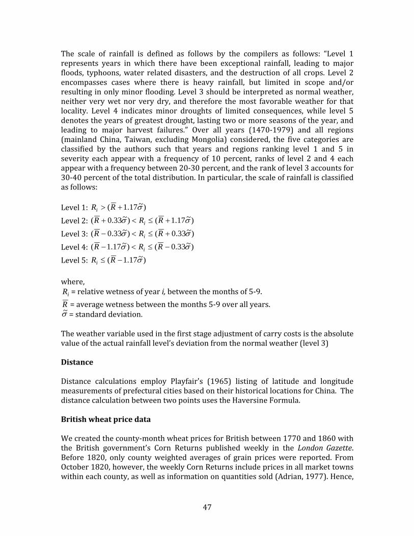
47

The scale of rainfall is defined as follows by the compilers as follows: “Level 1 represents years in which there have been exceptional rainfall, leading to major floods, typhoons, water related disasters, and the destruction of all crops. Level 2 encompasses cases where there is heavy rainfall, but limited in scope and/or resulting in only minor flooding. Level 3 should be interpreted as normal weather, neither very wet nor very dry, and therefore the most favorable weather for that locality. Level 4 indicates minor droughts of limited consequences, while level 5 denotes the years of greatest drought, lasting two or more seasons of the year, and leading to major harvest failures.” Over all years (1470-1979) and all regions (mainland China, Taiwan, excluding Mongolia) considered, the five categories are classified by the authors such that years and regions ranking level 1 and 5 in severity each appear with a frequency of 10 percent, ranks of level 2 and 4 each appear with a frequency between 20-30 percent, and the rank of level 3 accounts for 30-40 percent of the total distribution. In particular, the scale of rainfall is classified as follows: Level 1: Level 2: Level 3: Level 4: Level 5: where,

= relative wetness of year i, between the months of 5-9. = average wetness between the months 5-9 over all years. = standard deviation.

The weather variable used in the first stage adjustment of carry costs is the absolute value of the actual rainfall level’s deviation from the normal weather (level 3) Distance Distance calculations employ Playfair's (1965) listing of latitude and longitude measurements of prefectural cities based on their historical locations for China. The distance calculation between two points uses the Haversine Formula. British wheat price data We created the county-month wheat prices for British between 1770 and 1860 with the British government’s Corn Returns published weekly in the London Gazette. Before 1820, only county weighted averages of grain prices were reported. From October 1820, however, the weekly Corn Returns include prices in all market towns within each county, as well as information on quantities sold (Adrian, 1977). Hence,

)~17.1( σ+> RRi

)~17.1()~33.0( σσ +≤<+ RRR i

)~33.0()~33.0( σσ +≤<− RRR i

)~33.0()~17.1( σσ −≤<− RRR i

)~17.1( σ−≤ RRi

iRRσ~

48

for the period 1821-1860, we construct the monthly prices as the weighted averages of prices across market towns, using quantities as weights. British weather data We use the precipitation reconstructions from Pauling et al. (2006) to obtain our rainfall data used for the British carry cost adjustment. Pauling et al. (2006) present seasonal precipitation reconstructions for European land areas on a 0.5·0.5 resolved grid between 1500 and 1900. We use the nearest data point to each county as the county precipitation, and aggregate the seasonal data to get the total annual precipitation. To make it comparable to the Chinese data, we normalize the British data according to the above Chinese official methodology to a 1-5 scale

49

Table A.1. Chinese regions Region No. Name

Prefecture name in pinyin Province

Province in pinyin

Yangzi Delta

Region No. Name

Prefecture name in pinyin Province

Province in pinyin

Yangzi Delta

1 奉天府 Fengtian Fu 奉天 Fengtian 46 绛州 Jiangzhou Zhilizhou 山西 Shanxi 2 錦州府 Jingzhou Fu 奉天 Fengtian 47 隰州直隶州 Xizhou Zhilizhou 山西 Shanxi 3 承德府 Chengde Fu 热河 Rehe 48 朔平府 Shuoping Fu 山西 Shanxi 4 济南府 Jinan Fu 山东 Shandong 49 宁武府 Ningwu Fu 山西 Shanxi 5 兖州府 Yanzhou Fu 山东 Shandong 50 霍州直隶州 Huozhou Zhilizhou 山西 Shanxi 6 东昌府 Dongchang Fu 山东 Shandong 51 归绥道 Guisui Dao 山西 Shanxi 7 青州府 Qingzhou Fu 山东 Shandong 52 开封府 Kaifeng Fu 河南 Henan 8 登州府 Dengzhou Fu 山东 Shandong 53 归德府 Guide Fu 河南 Henan 9 莱州府 Laizhou Fu 山东 Shandong 54 彰德府 Zhangde Fu 河南 Henan 10 泰安府 Taian Fu 山东 Shandong 55 卫辉府 Weihui Fu 河南 Henan 11 武定府 Wuding Fu 山东 Shandong 56 怀庆府 Huaiqing Fu 河南 Henan 12 曹州府 Caozhou Fu 山东 Shandong 57 河南府 Henan Fu 河南 Henan 13 济宁直隶州 Jining Zhilizhou 山东 Shandong 58 南阳府 Nanyang Fu 河南 Henan 14 沂州府 Yizhou Fu 山东 Shandong 59 汝宁府 Runing Fu 河南 Henan 15 临清直隶州 Linqing Zhilizhou 山东 Shandong 60 汝州 Ruzhou Zhilizhou 河南 Henan 16 顺天府 Shuntian Fu 直隶 Zhili 61 陈州府 Chenzhou Fu 河南 Henan 17 保定府 Baoding Fu 直隶 Zhili 62 许州直隶州 Xuzhou Zhilizhou 河南 Henan 18 永平府 Yongping Fu 直隶 Zhili 63 陕州直隶州 Shaanzhou Zhilizhou 河南 Henan 19 河间府 Hejian Fu 直隶 Zhili 64 光州直隶州 Guangzhou Zhilizhou 河南 Henan 20 正定府 Zhengding Fu 直隶 Zhili 65 西安府 Xi'an Fu 陕西 Shaanxi 21 顺德府 Shunde Fu 直隶 Zhili 66 延安府 Yan'an Fu 陕西 Shaanxi 22 广平府 Guangping Fu 直隶 Zhili 67 凤翔府 Fengxiang Fu 陕西 Shaanxi 23 大名府 Daming Fu 直隶 Zhili 68 汉中府 Hanzhong Fu 陕西 Shaanxi 24 冀州直隶州 Jizhou Zhilizhou 直隶 Zhili 69 兴安府 Xing'an Fu 陕西 Shaanxi 25 赵州直隶州 Zhaozhou Zhilizhou 直隶 Zhili 70 商州 Shangzhou Zhilizhou 陕西 Shaanxi 26 深州直隶州 Shenzhou Zhilizhou 直隶 Zhili 71 同州府 Tongzhou Fu 陕西 Shaanxi 27 定州直隶州 Dingzhou Zhilizhou 直隶 Zhili 72 乾州厅 Qianzhou Zhilizhou 陕西 Shaanxi 28 天津府 Tianjin Fu 直隶 Zhili 73 邠州 Binzhou Zhilizhou 陕西 Shaanxi 29 易州直隶州 Yizhou Zhilizhou 直隶 Zhili 74 鄜州 Fuzhou Zhilizhou 陕西 Shaanxi 30 遵化州直隶州 Zunhua Zhilizhou 直隶 Zhili 75 绥德州 Suide Zhilizhou 陕西 Shaanxi 31 宣化府 Xuanhua Fu 直隶 Zhili 76 榆林府 Yulin Fu 陕西 Shaanxi 32 太原府 Taiyuan Fu 山西 Shanxi 77 兰州府 Lanzhou Fu 甘肃 Gansu 33 平阳府 Pingyang Fu 山西 Shanxi 78 平凉府 Pingliang Fu 甘肃 Gansu 34 大同府 Datong Fu 山西 Shanxi 79 巩昌府 Gongchang Fu 甘肃 Gansu 35 潞安府 Luan Fu 山西 Shanxi 80 庆阳府 Qingyang Fu 甘肃 Gansu 36 汾州府 Fenzhou Fu 山西 Shanxi 81 宁夏府 Ningxia Fu 甘肃 Gansu 37 辽州直隶州 Liaozhou Zhilizhou 山西 Shanxi 82 西宁府 Xining Fu 甘肃 Gansu 38 沁州直隶州 Qinzhou Zhilizhou 山西 Shanxi 83 安西直隶州 Anxi Zhilizhou 甘肃 Gansu 39 泽州府 Zezhou Fu 山西 Shanxi 84 凉州府 Liangzhou Fu 甘肃 Gansu 40 平定州 Pingding Zhilizhou 山西 Shanxi 85 甘州府 Ganzhou Fu 甘肃 Gansu 41 忻州直隶州 Xinzhou Zhilizhou 山西 Shanxi 86 秦州直隶州 Qinzhou Zhilizhou 甘肃 Gansu 42 代州直隶州 Daizhou Zhilizhou 山西 Shanxi 87 阶州直隶州 Jiezhou Zhilizhou 甘肃 Gansu 43 保德州 Baode Zhilizhou 山西 Shanxi 88 肃州直隶州 Suzhou Zhilizhou 甘肃 Gansu 44 蒲州府 Puzhou Fu 山西 Shanxi 89 泾州直隶州 Jingzhou Zhilizhou 甘肃 Gansu 45 解州 Jiezhou Zhilizhou 山西 Shanxi 90 江宁府 Jiangning Fu 江苏 Jiangsu 1

50

Region No. Name

Prefecture name in pinyin Province

Province in pinyin

Yangzi Delta

Region No. Name

Prefecture name in pinyin Province

Province in pinyin

Yangzi Delta

91 苏州府 Suzhou Fu 江苏 Jiangsu 1 136 福宁府 Funing Fu 福建 Fujian 92 松江府 Songjiang Fu 江苏 Jiangsu 1 137 永春州 Yongchun Zhilizhou 福建 Fujian 93 常州府 Changzhou Fu 江苏 Jiangsu 1 138 龙岩州 Longyan Zhilizhou 福建 Fujian 94 镇江府 Zhenjiang Fu 江苏 Jiangsu 1 139 台湾府 Taiwan Fu 福建 Fujian 95 淮安府 Huaian Fu 江苏 Jiangsu 140 武昌府 Wuchang Fu 湖北 Hubei 96 扬州府 Yangzhou Fu 江苏 Jiangsu 141 汉阳府 Hanyang Fu 湖北 Hubei 97 徐州府 Xuzhou Fu 江苏 Jiangsu 142 安陆府 Anlu Fu 湖北 Hubei 98 太仓直隶州 Taicang Zhilizhou 江苏 Jiangsu 1 143 襄阳府 Xiangyang Fu 湖北 Hubei 99 海州直隶州 Haizhou Zhilizhou 江苏 Jiangsu 144 郧阳府 Yunyang Fu 湖北 Hubei 100 通州直隶州 Tongzhou Zhilizhou 江苏 Jiangsu 1 145 德安府 De'an Fu 湖北 Hubei 101 安庆府 Anqing Fu 安徽 Anhui 146 黄州府 Huangzhou Fu 湖北 Hubei 102 徽州府 Huizhou Fu 安徽 Anhui 147 荆州府 Jingzhou Fu 湖北 Hubei 103 宁国府 Ningguo Fu 安徽 Anhui 148 宜昌府 Yichang Fu 湖北 Hubei 104 池州府 Chizhou Fu 安徽 Anhui 149 施南府 Shinan Fu 湖北 Hubei 105 太平府 Taiping Fu 安徽 Anhui 150 荆门直隶州 Jingmen Zhilizhou 湖北 Hubei 106 庐州府 Luzhou Fu 安徽 Anhui 151 长沙府 Changsha Fu 湖南 Hunan 107 凤阳府 Fengyang Fu 安徽 Anhui 152 岳州府 Yuezhou Fu 湖南 Hunan 108 广德直隶州 Guangde Zhilizhou 安徽 Anhui 153 宝庆府 Baoqing Fu 湖南 Hunan 109 和州直隶州 Hezhou Zhilizhou 安徽 Anhui 154 衡州府 Hengzhou Fu 湖南 Hunan 110 滁州直隶州 Chuzhou Zhilizhou 安徽 Anhui 155 常德府 Changde Fu 湖南 Hunan 111 六安州直隶州 Liu'an Zhilizhou 安徽 Anhui 156 辰州府 Chenzhou Fu 湖南 Hunan 112 泗州直隶州 Sizhou Zhilizhou 安徽 Anhui 157 永州府 Yongzhou Fu 湖南 Hunan 113 颍州府 Yingzhou Fu 安徽 Anhui 158 靖州 Jingzhou Zhilizhou 湖南 Hunan 114 南昌府 Nanchang Fu 江西 Jiangxi 159 郴州直隶州 Chenzhou Zhilizhou 湖南 Hunan 115 饶州府 Raozhou Fu 江西 Jiangxi 160 永顺府 Yongshun Fu 湖南 Hunan 116 广信府 Guangxin Fu 江西 Jiangxi 161 澧州直隶州 Lizhou Zhilizhou 湖南 Hunan 117 南康府 Nankang Fu 江西 Jiangxi 162 沅州府 Yuanzhou Fu 湖南 Hunan 118 九江府 Jiujiang Fu 江西 Jiangxi 163 桂阳州 Guiyang Zhilizhou 湖南 Hunan 119 建昌府 Jianchang Fu 江西 Jiangxi 164 广州府 Guangzhou Fu 广东 Guangdong 120 抚州府 Fuzhou Fu 江西 Jiangxi 165 韶州府 Shaozhou Fu 广东 Guangdong 121 临江府 Linjiang Fu 江西 Jiangxi 166 南雄直隶州 Nanxiong Zhilizhou 广东 Guangdong 122 吉安府 Ji'an Fu 江西 Jiangxi 167 惠州府 Huizhou Fu 广东 Guangdong 123 瑞州府 Ruizhou Fu 江西 Jiangxi 168 潮州府 Chaozhou Fu 广东 Guangdong 124 袁州府 Yuanzhou Fu 江西 Jiangxi 169 肇庆府 Zhaoqing Fu 广东 Guangdong 125 赣州府 Ganzhou Fu 江西 Jiangxi 170 高州府 Gaozhou Fu 广东 Guangdong 126 南安府 Nan'an Fu 江西 Jiangxi 171 廉州府 Lianzhou Fu 广东 Guangdong 127 宁都直隶州 Ningdu Zhilizhou 江西 Jiangxi 172 雷州府 Leizhou Fu 广东 Guangdong 128 福州府 Fuzhou Fu 福建 Fujian 173 琼州府 Qiongzhou Fu 广东 Guangdong 129 泉州府 Quanzhou Fu 福建 Fujian 174 罗定直隶州 Luoding Zhilizhou 广东 Guangdong 130 建宁府 Jianning Fu 福建 Fujian 175 连州直隶州 Lianzhou Zhilizhou 广东 Guangdong 131 延平府 Yanping Fu 福建 Fujian 176 嘉应直隶州 Jiaying Zhilizhou 广东 Guangdong 132 汀州府 Tingzhou Fu 福建 Fujian 177 佛冈直隶厅 Fogang Zhiliting 广东 Guangdong 133 兴化府 Xinghua Fu 福建 Fujian 178 连山直隶厅 Lianshan Zhiliting 广东 Guangdong 134 邵武府 Shaowu Fu 福建 Fujian 179 桂林府 Guilin Fu 广西 Guangxi 135 漳州府 Zhangzhou Fu 福建 Fujian 180 柳州府 Liuzhou Fu 广西 Guangxi

51

Region No. Name

Prefecture name in pinyin Province

Province in pinyin

Yangzi Delta

Region No. Name

Prefecture name in pinyin Province

Province in pinyin

Yangzi Delta

182 思恩府 Si'en Fu 广西 Guangxi 218 楚雄府 Chuxiong Fu 云南 Yunan 183 平乐府 Pingle Fu 广西 Guangxi 219 澂江府 Chengjiang Fu 云南 Yunan 184 梧州府 Wuzhou Fu 广西 Guangxi 220 广西直隶州 Guangxi Zhilizhou 云南 Yunan 185 浔州府 Xunzhou Fu 广西 Guangxi 221 顺宁府 Shunning Fu 云南 Yunan 186 南宁府 Nanning Fu 广西 Guangxi 222 曲靖府 Qujing Fu 云南 Yunan 187 太平府 Taiping Fu 广西 Guangxi 223 武定直隶州 Wuding Zhilizhou 云南 Yunan 188 郁林直隶州 Yulin Zhilizhou 广西 Guangxi 224 永昌府 Yongchang Fu 云南 Yunan 189 泗城府 Sicheng Fu 广西 Guangxi 225 永北直隶厅 Yongbei Zhiliting 云南 Yunan 190 镇安府 Zhenan Fu 广西 Guangxi 226 元江直隶州 Yuanjiang Zhilizhou 云南 Yunan 191 成都府 Chengdu Fu 四川 Sichuan 227 广南府 Guangnan Fu 云南 Yunan 192 保宁府 Baoning Fu 四川 Sichuan 228 蒙化直隶厅 Menghua Zhiliting 云南 Yunan 193 顺庆府 Shunqing Fu 四川 Sichuan 229 景东直隶厅 Jingdong Zhiliting 云南 Yunan 194 叙州府 Xuzhou Fu 四川 Sichuan 230 开化府 Kaihua Fu 云南 Yunan 195 重庆府 Zhongqing Fu 四川 Sichuan 231 丽江府 Lijiang Fu 云南 Yunan 196 夔州府 Kuizhou Fu 四川 Sichuan 232 东川府 Dongchuan Fu 云南 Yunan 197 龙安府 Longan Fu 四川 Sichuan 233 镇沅直隶州 Zhenyuan Zhiliting 云南 Yunan 198 潼川府 Tongchuan Fu 四川 Sichuan 234 昭通府 Zhaotong Fu 云南 Yunan 199 嘉定府 Jiading Fu 四川 Sichuan 235 普洱府 Puer Fu 云南 Yunan 200 雅州府 Yazhou Fu 四川 Sichuan 236 镇雄直隶州 Zhenxiong Zhilizhou 云南 Yunan 201 眉州 Meizhou Zhilizhou 四川 Sichuan 237 贵阳府 Guiyang Fu 贵州 Guizhou 202 邛州 Qiongzhou Zhilizhou 四川 Sichuan 238 思州府 Sizhou Fu 贵州 Guizhou 203 泸州直隶州 Luzhou Zhilizhou 四川 Sichuan 239 思南府 Sinan Fu 贵州 Guizhou 204 资州 Zizhou Zhilizhou 四川 Sichuan 240 镇远府 Zhenyuan Fu 贵州 Guizhou 205 绵州 Mianzhou Zhilizhou 四川 Sichuan 241 石阡府 Shiqian Fu 贵州 Guizhou 206 茂州 Maozhou Zhilizhou 四川 Sichuan 242 铜仁府 Tongren Fu 贵州 Guizhou 207 叙永厅 Xuyong Zhilizhou 四川 Sichuan 243 黎平府 Liping Fu 贵州 Guizhou 208 绥定府 Suiding Fu 四川 Sichuan 244 安顺府 Anshun Fu 贵州 Guizhou 209 宁远府 Ningyuan Fu 四川 Sichuan 245 都匀府 Duyun Fu 贵州 Guizhou 210 酉阳州 Youyang Zhilizhou 四川 Sichuan 246 平越直隶州 Pingyue Zhilizhou 贵州 Guizhou 211 忠州 Zhongzhou Zhilizhou 四川 Sichuan 247 大定府 Dading Fu 贵州 Guizhou 212 松潘厅 Songpan Zhiliting 四川 Sichuan 248 兴义府 Xingyi Fu 贵州 Guizhou 213 石砫厅 Shizhu Zhiliting 四川 Sichuan 249 遵义府 Zunyi Fu 贵州 Guizhou 214 太平厅 Taiping Zhiliting 四川 Sichuan 250 仁怀直隶厅 Renhuai Zhiliting 贵州 Guizhou 215 云南府 Yunnan Fu 云南 Yunan 251 松桃直隶厅 Songtao Zhiliting 贵州 Guizhou 216 大理府 Dali Fu 云南 Yunan 252 普安直隶厅 Pu'an Zhiliting 贵州 Guizhou 217 临安府 Lin'an Fu 云南 Yunan

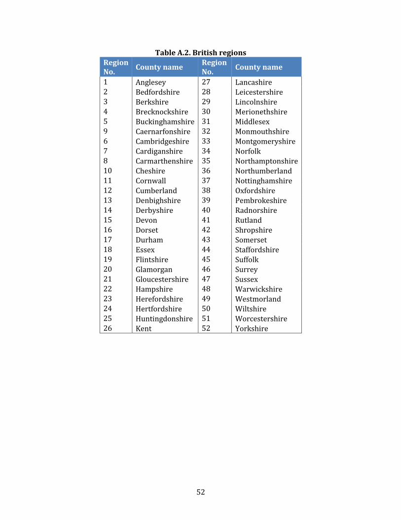
52

Table A.2. British regions Region No. County name Region

No. County name

1 Anglesey 27 Lancashire 2 Bedfordshire 28 Leicestershire 3 Berkshire 29 Lincolnshire 4 Brecknockshire 30 Merionethshire 5 Buckinghamshire 31 Middlesex 9 Caernarfonshire 32 Monmouthshire 6 Cambridgeshire 33 Montgomeryshire 7 Cardiganshire 34 Norfolk 8 Carmarthenshire 35 Northamptonshire 10 Cheshire 36 Northumberland 11 Cornwall 37 Nottinghamshire 12 Cumberland 38 Oxfordshire 13 Denbighshire 39 Pembrokeshire 14 Derbyshire 40 Radnorshire 15 Devon 41 Rutland 16 Dorset 42 Shropshire 17 Durham 43 Somerset 18 Essex 44 Staffordshire 19 Flintshire 45 Suffolk 20 Glamorgan 46 Surrey 21 Gloucestershire 47 Sussex 22 Hampshire 48 Warwickshire 23 Herefordshire 49 Westmorland 24 Hertfordshire 50 Wiltshire 25 Huntingdonshire 51 Worcestershire 26 Kent 52 Yorkshire

53

Figure A.1. Filtered versus unfiltered Philadelphia wheat prices, 1836-40

Notes: Data for unfiltered series is from Jacks (2006); filtered series is own calculation.

-0.15

-0.1

-0.05

0

0.05

0.1

0.15

1.00

1.20

1.40

1.60

1.80

2.00

2.20

2.40

Jan-

1836

Mar

-183

6M

ay-1

836

Jul-

1836

Sep-

1836

Nov

-183

6Ja

n-18

37M

ar-1

837

May

-183

7Ju

l-18

37Se

p-18

37N

ov-1

837

Jan-

1838

Mar

-183

8M

ay-1

838

Jul-

1838

Sep-

1838

Nov

-183

8Ja

n-18

39M

ar-1

839

May

-183

9Ju

l-18

39Se

p-18

39N

ov-1

839

Jan-

1840

Mar

-184

0M

ay-1

840

Jul-

1840

Sep-

1840

Nov

-184

0

Bu

tter

wor

th-f

ilte

red

log

pri

ce p

er b

ush

el

log

pri

ce p

er b

ush

el

Unfiltered Butterworth band-pass filtered