NBER WORKING PAPER SERIES

BUBBLES AND BUSTS: THE 1990s IN THE MIRROR OF THE 1920s

Eugene N. White

Working Paper 12138http://www.nber.org/papers/w12138

NATIONAL BUREAU OF ECONOMIC RESEARCH1050 Massachusetts Avenue

Cambridge, MA 02138March 2006

The author is Professor of Economics, Rutgers University, New Brunswick, New Jersey 08901 and ResearchAssociate of the National Bureau of Economic Research. A preliminary version of this paper was presentedat Understanding the 1990s: The Long-Run Perspective at Duke University in October 2004. Comments fromseminar participants and subsequent seminars at the University of Copenhagen, the Swedish School ofEconomics, the Bank of Spain, and the University of Venice are gratefully acknowledged. The viewsexpressed herein are those of the author(s) and do not necessarily reflect the views of the National Bureauof Economic Research.

©2006 by Eugene N. White. All rights reserved. Short sections of text, not to exceed two paragraphs, maybe quoted without explicit permission provided that full credit, including © notice, is given to the source.

Bubbles and Busts: The 1990s in the Mirror of the 1920sEugene N. WhiteNBER Working Paper No. 12138March 2006JEL No. E5, G1, N1, N2

ABSTRACT

This paper surveys the twentieth century booms and crashes in the American stock market, focusingon a comparison of the two most similar events in the 1920s and 1990s. In both booms, claims weremade that they were the consequence a “new economy” or “irrational exuberance.” Neither boomcan be readily explained by fundamentals, represented by expected dividend growth or changes inthe equity premium. The difficulty of identifying the fundamentals implies that central banks wouldnot be successful in preventing pre-emptive policies, although they still would have a critical roleto play in preventing crashes from disrupting the payments system or sparking an intermediationcrisis.

Eugene N. WhiteDepartment of EconomicsRutgers UniversityNew Brunswick, NJ 08901and NBERwhite@economics.rutgers.edu

2

“History is continually repudiated.” -Glassman and Hassett (1999) The Dow 36,000

Stock market booms and busts command enormous attention, yet there is little

consensus about their causes and effects. The soaring market of the 1990s was seen by

many, but certainly not all, as the harbinger of a new age of sustained, rapid economic

growth. Optimists saw the bull market as driven by fundamentals, although they differed

over what these were; while skeptics warned that it was just a bubble, distorting

consumption and investment decisions. Regardless of the boom’s origin, policy makers

feared that a collapse would have real economic consequences and debated how to cope

with the market’s retreat.

Although the sheer size of the run up in stock prices in the 1990s has obscured

other bull markets in the popular eye, the boom shared many characteristics with previous

episodes, notably the 1920s; and the explanations and policy concerns were similar. As in

the 1990s, it was widely claimed that a “new economy” had taken root in the U.S.

Technological and organizational innovations were viewed as raising productivity,

increasing firms’ earnings and justifying the wave of new issues. In both periods,

unemployment was low with stable prices in the twenties and very low inflation in the

nineties. Participation in the market increased, as investing in the market seemed safer,

with reduced macroeconomic risk and the seeming abundance of high return

opportunities.

Just as the new heights of the 1990s market were often challenged as the product

of “irrational exuberance,” so too there were critics of the fast surge in stock prices in

1928-1929. Policy makers were concerned about the distortions that the quick run up in

3

stock prices would have on the economy. The potential presence of an asset bubble

raised the question of the appropriate policy response---and in the 1920s the bull market

helped to produce a grievously mistaken monetary policy.

As booms and crashes are relatively rare events, this paper offers a comparison of

the 1920s and the 1990s to provide perspective on the question of whether the Federal

Reserve should respond to booms and crashes. The answer to this question depends

critically on the ability of policy makers to identify fundamental components in the stock

market. Although considerable energy has been expended to justify stock price

movement in terms of fundamentals and measure bubbles, it has proven to be an elusive

effort. While this pre-empts a policy response to a boom, the Fed still has a critical role

to play in preventing crashes from disrupting the payments system or sparking an

intermediation crisis.

DEFINING BOOMS AND CRASHES?

Some stock market booms and crashes are well remembered; but in general, these

events are imperfectly defined. While we typically think of the stock market as following

a random walk, a boom is viewed as an improbably long period of large positive returns

that is cast into sharp profile by a crash. The first questions to address are whether the

twenties and nineties stand out in comparison to other booms and crashes and whether

they shared similar characteristics?

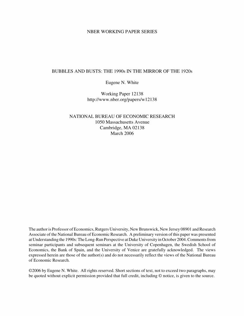
To identify booms, we need to look for long periods of positive real stock returns.

Figure 1 shows the annual real returns on the S&P 500 for 1871 to 2003.1 Annual data

provide the appropriate window to look for bull markets, as they are seen as long upward

4

swings that dominate any brief retreat that might be picked up in data of a higher

frequency. The bull market of 1995-1999 stands out, with returns of 27, 21, 22, 25 and

12%. If three consecutive years of returns over 10 percent is used as an approximate

criterion, booms are relatively rare. The first boom for this data is 1921-1928, which had

a long run of positive run returns of 20, 26, 2, 23, 19, 13, 32, and 39%. Next is 1942-

1945, where returns were 11, 18, 15 and 30%. The 1950s also had a long bull market

where there was a streak of positive returns: 18, 22, 15, 13, 2, 39, 25% from 1949 to

1956. The years 1963-1965 saw gains of 17, 13, and 9%, while 1982-1986 enjoyed

returns of 22, 14, 4, 19 and 26%. Few contemporaries seemed concerned that the booms

of the forties, fifties, or sixties left the market far out of alignment, and it is the fear of a

crash that identifies a bull market that singles out the 1920s, 1980s, and 1990s.

Mishkin and White (2003) developed a simple method for identifying crashes,

using the three most well known stock indices to capture the fortunes of different

segments of the market: the Dow Jones Industrials, Standard and Poor’s (S&P) 500 and

its predecessor the Cowles Index, and the Nasdaq. Since October 1929 and October 1927

are universally agreed to be stock market crashes, they were used as benchmarks. In both

cases, the market fell over 20 percent in one and two days’ time. The fall in the market,

or the depth, is only one characteristic of a crash. There was no similar sudden decline

for the most recent collapse, but no one would hesitate to identify 2000 as the beginning

of a major collapse. Thus, speed is another feature. To identify crashes, it is necessary to

look at windows of one day, one week, one month and one year to capture other declines.

1 The most frequently used data for examining booms, crashes and bubbles are the series on Robert Shiller’s webpage, http://www.econ.yale.edu/~shiller/data.htm, where the return is ln(1 + real return), where the return includes dividends and the capital gain.

5

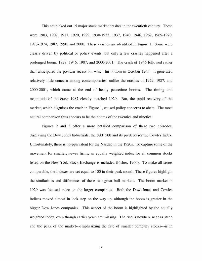
This net picked out 15 major stock market crashes in the twentieth century. These

were 1903, 1907, 1917, 1920, 1929, 1930-1933, 1937, 1940, 1946, 1962, 1969-1970,

1973-1974, 1987, 1990, and 2000. These crashes are identified in Figure 1. Some were

clearly driven by political or policy events, but only a few crashes happened after a

prolonged boom: 1929, 1946, 1987, and 2000-2001. The crash of 1946 followed rather

than anticipated the postwar recession, which hit bottom in October 1945. It generated

relatively little concern among contemporaries, unlike the crashes of 1929, 1987, and

2000-2001, which came at the end of heady peacetime booms. The timing and

magnitude of the crash 1987 closely matched 1929. But, the rapid recovery of the

market, which disguises the crash in Figure 1, caused policy concerns to abate. The most

natural comparison thus appears to be the booms of the twenties and nineties.

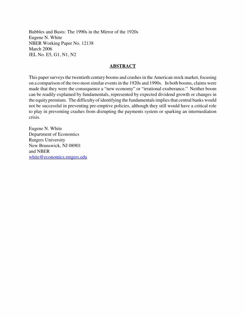
Figures 2 and 3 offer a more detailed comparison of these two episodes,

displaying the Dow Jones Industrials, the S&P 500 and its predecessor the Cowles Index.

Unfortunately, there is no equivalent for the Nasdaq in the 1920s. To capture some of the

movement for smaller, newer firms, an equally weighted index for all common stocks

listed on the New York Stock Exchange is included (Fisher, 1966). To make all series

comparable, the indexes are set equal to 100 in their peak month. These figures highlight

the similarities and differences of these two great bull markets. The boom market in

1929 was focused more on the larger companies. Both the Dow Jones and Cowles

indices moved almost in lock step on the way up, although the boom is greater in the

bigger Dow Jones companies. This aspect of the boom is highlighted by the equally

weighted index, even though earlier years are missing. The rise is nowhere near as steep

and the peak of the market---emphasizing the fate of smaller company stocks---is in

6

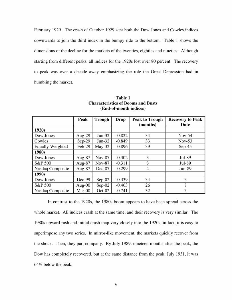
February 1929. The crash of October 1929 sent both the Dow Jones and Cowles indices

downwards to join the third index in the bumpy ride to the bottom. Table 1 shows the

dimensions of the decline for the markets of the twenties, eighties and nineties. Although

starting from different peaks, all indices for the 1920s lost over 80 percent. The recovery

to peak was over a decade away emphasizing the role the Great Depression had in

humbling the market.

Table 1

Characteristics of Booms and Busts (End-of-month indices)

Peak Trough Drop Peak to Trough

(months) Recovery to Peak

Date 1920s Dow Jones Aug-29 Jun-32 -0.822 34 Nov-54 Cowles Sep-29 Jun-32 -0.849 33 Nov-53 Equally-Weighted Feb-29 May-32 -0.896 39 Sep-45 1980s Dow Jones Aug-87 Nov-87 -0.302 3 Jul-89 S&P 500 Aug-87 Nov-87 -0.311 3 Jul-89 Nasdaq Composite Aug-87 Dec-87 -0.299 4 Jun-89 1990s Dow Jones Dec-99 Sep-02 -0.339 34 ? S&P 500 Aug-00 Sep-02 -0.463 26 ? Nasdaq Composite Mar-00 Oct-02 -0.741 32 ?

In contrast to the 1920s, the 1980s boom appears to have been spread across the

whole market. All indices crash at the same time, and their recovery is very similar. The

1980s upward rush and initial crash map very closely into the 1920s, in fact, it is easy to

superimpose any two series. In mirror-like movement, the markets quickly recover from

the shock. Then, they part company. By July 1989, nineteen months after the peak, the

Dow has completely recovered, but at the same distance from the peak, July 1931, it was

64% below the peak.

7

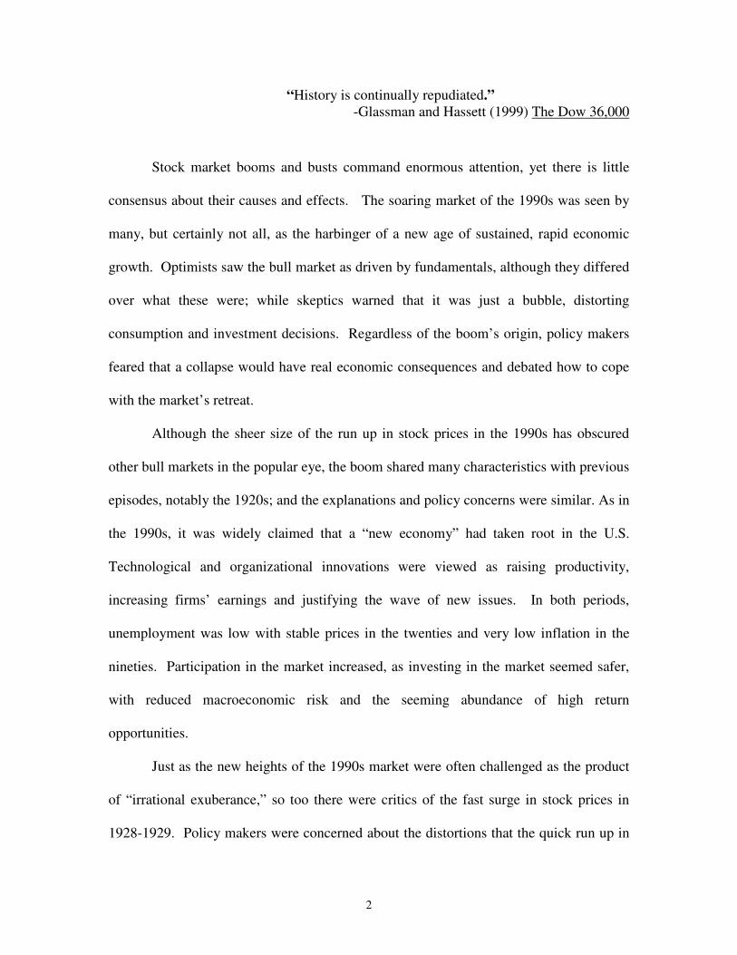
The rising tide of the 1990s lifted all boats, but the high tech, small company

stocks of the Nasdaq rode the crest. In comparison to the 1920s when large companies

dominated the rising market or the 1980s when all rose together, the Nasdaq firms were

the center of the boom, rising higher and falling further. The collapse of the “tech

bubble” looks more like the busts of October 1929 and October 1987. From the peak in

March 2000, the Nasdaq lost 20% within a month. The jagged slump from peak to

trough produced a loss of 74%; the size and timing matching the collapse from 1929. In

Table 1, the larger, more established companies represented by the Dow Jones and the

S&P 500 experienced the same magnitude of loss as did the indices in 1987 and the

initial decline from August to November 1929; but it is slower and more gradual. By the

end of 2003, all three indices had recovered partly but with markedly different success.

The absence of a quick recovery à la 1987 and the magnitude of duration of Nasdaq’s

collapse make the twenties and nineties a natural comparison.

BUBBLES OR FUNDAMENTALS?

Discussion of booms and busts sharply divide observers. There are those who

believe that fundamentals are solely responsible for the movements in stock prices and

those who believe that stock prices are largely detached from fundamentals, moved by

the fluctuating optimism and pessimism of investors.

Looking back on the boom and bust of the 1920s, Professor John B. Williams of

Harvard wrote:

Like a ghost in a haunted house, the notion of a soul possessing the market and sending it up or down with a shrewdness uncanny and superhuman,

8

keeps ever reappearing….Let us define the investment value of a stock as the present worth of all the dividends to be paid upon it (Williams, 1938).

Viewing the same period, John Maynard Keynes chose to differ:

A conventional valuation which is established as the outcome of the mass psychology of a large number of ignorant individuals is liable to change violently as the result of a sudden fluctuation of opinion which do not really make much difference to the prospective yield…..the market will be subject to waves of optimistic and pessimistic sentiment, which are unreasoning (Keynes, 1936).

On the threshold of the great bull market, the divide remained. Robert Shiller observed:

I present here evidence that while some of the implications of the efficient markets hypothesis are substantiated by data, investor attitudes are of great importance in determining the course of prices of speculative assets. Prices change in substantial measure because the investing public en masse capriciously changes its mind (Shiller, 1991).

In contrast, John Cochrane expounded:

We can still argue over what name to attach to residual discount-rate movement. Is it variation in real investment opportunities not captured by current discount model? Or is it “fads?” I argue that residual discount-rate variation is small (in a precise sense), and tantalizingly suggestive of economic explanation. I argue that “fads are just a catchy name for the residual (Cochrane, 1991).

These extreme positions can be maintained because of the observational

equivalence in any empirical test between a market driven by a bubble and one where it is

driven by fundamentals but there are omitted factors (Flood and Hodrick, 1990). Most

models of market behavior are based on rational expectations, which assumes that (1)

individuals have rational information processing and (2) individuals have a correct model

of the fundamental structure of the economy. Bubbles or manias may arise if either

condition is violated. If the first is violated, there will be an irrational bubble or mania;

and if the second is violated, there will be a rational bubble. With either violation, asset

prices will deviate from fundamentals (Blanchard and Watson, 1982). In rational

9

bubbles, market participants may have rational expectations but prices may differ from

fundamentals because the sequence of prices in rational expectations models may be

indeterminate. Bubbles will be rational as long as the bubble component in the stock

price is the expected discounted value of the future bubble. In an irrational bubble,

market participants may focus on “noise” instead of fundamentals. Some noise or

unsophisticated traders in a market may overwhelm rational or sophisticated investors if

the time horizons for arbitrage are finite (De Long, Shleifer, Summers and Waldman,

1990). If share prices are moved by a bubble, it will induce distortions into the market,

mis-directing investment, policy intervention may be required.

FUNDAMENTALS AND EMPIRICAL REGULARITIES

What were the driving fundamental factors behind the great bull markets of the

1920s and 1990s? Even if one believes that a bubble or investor euphoria was the key

factor, the natural starting point is how to measure the contribution of fundamentals to

prices. Fundamentals require that stock prices equal the present discounted value of

expected future dividends. The simplest approximation to this fundamentals-based

valuation is the Gordon growth model, which underlies many studies and much popular

discussion. While expected future dividends and interest rates may vary considerably,

the simple Gordon model assumes constant values for all parameters. Dividends are

assumed to grow at a rate g and investors are assumed to require a return of a r,

composed of a risk free rate and an equity premium.2 Usually framed in terms of the

aggregate price level of the stock market, P, the Gordon model is:

2 If a constant fraction of earnings, E, are paid out as dividends, where b is the proportion of reinvested earnings, then D = (1-b)E.

10

(1) P = (1+g)D/(r-g)

While changes in the payout rate and the risk free rate may have contributed some to

upsurges in the market, it is technological change, increasing productivity and leading to

higher dividend growth, and changes in the equity premium that are believed to have

been the prime movers.

The Gordon model neatly outlines the simple fundamental relationship, yet

explaining stock price movements has proved frustratingly difficult. The problem is that

to be rational prices should be wholly forward looking, representing the expected future

course of dividends appropriately discounted. In a classic article, Shiller (1981) found

that stock prices moved far more than was warranted by the movement of dividends,

where the ex post rational price was equal to the discounted value of the future stream of

realized dividends. Even if there were deviations in what was expected from what was

realized, the fit should have been good over his long period of observation, 1871-1979;

yet the variation of prices exceeded the variation in fundamental prices violating any

reasonable test.3

While it has proven difficult to explain the behavior of prices in terms of the

movement of future dividends and discount rates, a very different literature has found

empirical regularities, explaining the behavior of current prices in terms of past

fundamentals. This predictability is surprising, given that prices should be forward

looking; and it provides a further instrument for analyzing the unusual behavior of prices

during stock market booms. Fama and French (1988) found that both the lagged dividend

3 Critics attacked the small sample properties of Shiller’s tests and his methods of detrending (Flavin, 1983; Kleidon, 1986) but in a survey West (1988) concluded that Shiller’s results were reasonably robust against these and other criticisms.

11

yield and the lagged earnings yield had explanatory power for stock returns.4 Lamont

(1998) has argued that high dividends predict high future returns because dividends

measure the permanent component of stock prices, reflecting the dividend policy of

managers. The payout ratio (dividend-earnings ratio) forecasts returns because the level

of earnings is a measure of current business conditions.5 It is generally observed that

investors required high stock returns in recessions and low returns in booms, and risk

premia on stocks covary with the business cycle. As earnings vary with the business

cycle, current earnings forecasts future returns, thus both dividends and earnings have

information for stock returns. However, the variation explained by these models is very

modest.

Table 2 gives a closer look at the key ratios for each of the boom periods. Real

dividends and earnings climbed to historic highs in 1928-1929, but the market rose so

much that the dividend yield and earnings to price ratio fell below traditional levels, and

the payout ratio moved back to an earlier level. If these two years represented a new era,

with higher earnings paying out higher dividends but with a greater share being

reinvested, then optimists would seem to have had good cause for paying higher stock

prices. Yet, from the empirical regularities, we would anticipate that the fall in the

dividend yield would reduce future returns, with the falling earnings price ratio

mitigating it to some degree. For the 1990s, the picture was somewhat different. Real

earnings per share jumped, but little was paid out in dividends. Again, the market’s surge

caused both measures to collapse to unprecedented lows; and the abrupt rise in the market

was not anticipated empirically by the changes in the key ratios.

4 See also Campbell and Shiller (1988).

12

Table 2

The Dividend Yield, Earnings to Price Ratio and Payout Ratio in Two Booms

Real

Dividends Dividend Yield

Real Earnings

Earnings To Price

Payout Ratio

Real Price

1900-1909 7.6 4.6 12.7 7.6 60.4 173.1 1910-1919 8.0 5.9 13.5 10.1 62.4 149.6 1920-1924 5.3 6.3 7.6 8.8 81.9 83.5

1925 6.1 5.7 12.7 11.8 48.0 110.9 1926 7.1 5.5 12.8 9.8 55.6 128.1 1927 8.1 5.7 11.6 8.3 69.4 138.8 1928 9.0 4.8 14.6 7.9 61.6 183.7 1929 10.3 3.9 17.1 6.5 60.2 263.6 1930 11.2 4.5 11.1 4.5 101.0 230.2 1931 10.4 5.1 7.7 3.8 134.4 182.2 1932 7.0 6.0 5.8 4.9 122.0 105.2 1933 6.0 6.2 6.0 6.2 100.0 99.6

1970-1979 13.2 4.1 29.4 9.4 45.5 360.9 1980-1989 13.5 4.6 28.1 9.5 48.6 321.5 1990-1994 15.9 3.2 27.6 5.4 59.8 521.7

1995 16.2 3.0 39.9 7.3 40.6 561.2 1996 17.0 2.4 44.1 6.3 38.5 721.5 1997 17.4 2.0 44.6 5.2 39.0 873.1 1998 17.9 1.7 41.6 3.9 43.0 1080.8 1999 17.9 1.3 51.7 3.9 34.6 1378.0 2000 16.8 1.1 51.8 3.5 32.5 1531.2 2001 16.1 1.2 25.3 1.9 63.8 1378.1 2002 15.8 1.4 30.3 2.7 52.1 1167.3

Source: Robert Shiller’s webpage, http://www.econ.yale.edu/~shiller/data.htm In a telling out-of-sample exercise at the outset of the nineties, Lamont (1998)

forecast the cumulative return of buying stocks on December 31, 1994. For his sample

period (1947-1994), the unconditional mean excess return over a five year period was

33%. But using a VAR regression with a starting point of December 31, 1994, the out-

of-sample forecast was one percent below total Treasury bills returns to 2000! Even with

a potential total forecast error of 21 percent this was well below the performance of the

market. His conclusion was that in the mid-1990s, U.S. stock prices were very high

5 One concern about using dividends to forecast returns is if stock repurchases replace dividends then past

13

relative to any benchmark. The surprising failure of stock prices to conform to some

simple rational model or the empirical regularities requires a closer examination of the

fundamentals components of the Gordon model.

EXPLANATION: TECHNOLOGICAL CHANGE

In both the 1920s and the 1990s, many bulls heralded the arrival of a “new”

economy. They saw a higher rate of technological change as the driving force behind a

faster growing economy and a rapidly rising stock market. Surging initial public

offerings, many based on technological or managerial innovations, flooded the markets in

both periods. Technological innovations were viewed as improving the marginal product

of capital, increasing earnings and hence dividend growth. A wave of innovations,

sometimes characterized as a new general purpose technology was believed to have

placed the economy on a higher growth path.

In New Levels in the Stock Market (1929), Charles Amos Dice Ohio State argued

that higher stock prices were the product of higher productivity. Dice identified

increased expenditure on research and development and the application of modern

management methods as prime factors behind the boom. Irving Fisher (1930) saw the

stock market boom as justified by the rise in earnings, driven by the systematic

application of science and invention in industry and the acceptance of the new industrial

management methods of Frederick Taylor. But not everyone was so sanguine. A.P.

Giannini, head of Bancitaly (the future Bank of America) stated in 1928 that the high

price of his bank’s stock was unwarranted given the planned dividends. Management of

history of dividend yields and payout ratios will not be a good guide to stock returns.

14

some high flying companies, including Canadian Marconi and Brooklyn Edison, also

became alarmed and announced that their shares were overvalued (Patterson, 1965).

As suggested by the relatively stronger performance of the largest companies in

the stock indices in Figure 2, the boom of the 1920s was centered on large-scale

commercial and industrial enterprises that took advantage of continuous-process

technologies. These were coordinated by the emerging system of modern management

that produced more efficient vertically-integrated enterprises, capturing economies of

scale and scope (Chandler, 1977). Among the “new” industries were automobiles. The

Ford Motor Company had pioneered mass production techniques, but General Motors

developed a diversified line of production and a more advanced management and

organization system, becoming the industry leader. GM’s president predicted that its

stock price would rise from 180 to 225 and he promised to return 60 percent of earnings

to stockholders.

Other new technology industries included radio, movies, aircraft, electric utilities

and banking. Like many fast-growing companies, RCA did not pay dividends but

reinvested its earnings. Other prominent new technology companies were Radio-Keith

Orpheum, the United Aircraft and Transport Corporation, and the Aluminium Company

of America. Central to many of the new technologies was the electricity industry, which

was transformed in the 1920s. Utilities had been local industries, but there were now

technological opportunities to gain economies of scale in production and transmission,

providing incentives to consolidate the industry. In a wave of mergers, banks expanded

and acquired other types of financial institutions to provide a wide range of services,

yielding advantages of scale and scope. Stock indices available for utilities and banking

15

outstripped the Dow Jones and S&P500 indices, much as the tech company stock indices

of the 1990s did.

Some students of the 1920s have sought to explain the boom as primarily driven

by technological change raising dividends. Sirkin (1975) applied a version of the Gordon

model to Dow Jones stocks in the 1920s to see if price-earnings ratios could have been

justified by a temporarily higher growth of earnings. Price-earnings ratios had ranged

between 12 to 15 before the bull market, while the mean and median at the peak in 1929

were 24.3 and 20.4. Assuming a fixed discount rate of 9%, Sirkin calculated the higher

earnings growth and number of years that would be needed to justify peak price earnings

ratios. In his best case, if the higher growth rate of 8.9% typical of 1925-1929 had been

sustained for ten years, a price-earnings ratio of 20.4 would have been justified or over

justified; thus he concluded that the market was not overvalued.

Although simple, Sirkin’s study is fairly typical of many non-nested exercises

devised to explain the booms of the 1920s and 1990s, which focus on one variable.

Sirkin’s results are also sensitive to the selection of 1925-1929 as a time frame for high

sustainable earnings. If the years 1927-1929 were selected to measure reasonable future

earnings growth, all price-earnings ratios he examined would have been justified. This

point reflects the fact that earnings are highly variable, compared with the permanent

component of dividends.

Donaldson and Kamstra (1996) sought a similar explanation for the 1929 boom

and bust, focusing on changes in the expected growth of dividends. In the simple Gordon

growth model, dividend growth cannot explain the price peak. Prices moved far away

from their fundamentals, and simple tests show that one cannot reject the presence of a

16

bubble. However, using pre-1920 dividend data, Donaldson and Kamstra estimated a

non-linear ARMA-ARCH model for discounted dividend growth and found that out-of-

sample forecasts produce a fundamental price series with a similar time pattern to the

actual S&P index. The fit is so close that it is hard to reject expected dividend growth as

the driving factor. Yet, the discount rate plays no significant role. While Donaldson and

Kamstra used alternatively a constant discount rate and a variable one, they do not allow

for any significant variation in the equity premium, a key feature of the boom. Close

inspection of their charts reveals that their fundamental peak follows the actual peak,

suggesting that the fit may partly reflect the highly persistent behavior of dividends.

In contrast to Sirkin and Donaldson and Kamstra, Barrie Wigmore (1985) saw no

evidence in earnings that could justify the run up in stock prices. In his detailed survey of

the behavior of individual stocks, he pointed out that at the market’s peak stock prices

average 30 times 1929 earnings up from 10 and at most 20 before the boom. Although

30 was the average, many stocks fell in the 30-50 range, with a number over 100. He

concluded that “such stock prices were clearly dependent on further price rises rather

than on the income generated and distributed by companies.…as the low returns on

equity show, these high valuations placed little emphasis on earnings.”6

The idea of a new technological age played a key role in the mind of the 1990s’

bull market. The rapid changes in computer/information technology and biotechnology

were heralded as placing the economy of a higher trajectory. This “new era” vision was

supported by some economists. Comparing the computer revolution to the introduction

and spread of electricity and internal combustion, Jovanovic and Rousseau (2002)

projected that this general purpose technology would have an even greater impact on

17

productivity growth. Prices for electricity and automobiles had declined sharply in the

1910s and 1920s, and most quickly after 1924, suggesting a key role for technology in

the boom of the 1920s. But, price declines for information technology produces have

been much faster, promising higher levels of growth and consumption.

Yet, this rosy future is not strongly supported by more general studies of

productivity growth. In a reassessment of long-term multi-factor productivity (MFP)

growth, Gordon (June 2000) painted a broad picture of slow growth in the nineteenth

century. From an average annual growth rate of 0.39% for 1870-1891, MFP began to

climb, hitting 1.14% for 1890-1913. After World War I, it continued its upward

movement, rising to 1.42% for 1913-1928 before cresting at 1.90% in 1928-1950.

Gordon argued that this peak of MFP growth was attributable to a cluster of four

inventions: electricity, the internal combustion engine, petrochemicals-plastics-

pharmaceuticals, and communications-entertainment (telegraph, telephone, radio,

movies, television, recorded music and mass-circulation newspapers and magazines).

These were all well established before World War II, except for television, and their

diffusion and improvements thus contributed to the peak of MFP growth of 1928-1950.

MFP growth subsided to 1.47% for 1950-1964 and then plummeted to 0.89% for 1964-

1972, hitting bottom at 0.16% for 1972-1979. The recovery to 0.59% in 1979-1988 and

0.79% for 1988-1996 remained far below the peak, leading Gordon to conclude that the

contributions from the four earlier general purpose technologies dwarfed today’s

technology information computer/chip-based IT revolution. Gordon (August 2000)

found the most recent increase in MFP for 1995-1999 to be 1.35%, consisting of a 0.54

unsustainable cyclical effect and 0.81% in trend growth which he attributed wholly to the

6 Wigmore, p. 382.

18

computer-IT sector. For the remainder of the economy, MFP did not revive, and outside

of durables it actually decelerated.7 The differences in productivity growth in the late

1990s between IT industries and the rest of the economy look like a potentially good

explanation for the greater buoyancy of the Nasdaq compared to the rest of the market.

Certainly, it would explain investor response to developments in the IT industry.

However, the boom outside of the new economy appears surprising without a major

increase in productivity growth, giving skeptics ammunition.

The implications of the modest increase in productivity growth for the value of

stocks is found in Heaton and Lucas’(1999) study, which parallels Sirkin’s exercise for

the 1920s. They calculated the growth rates that would be needed to justify the peak

price-dividend using Shiller’s annual data (1872-1998). For this 126 year period, the

average price-dividend ratio was 28 and real earnings growth rate was 1.4%, implying a

discount rate of 5%.8 To match the 1998 ratio of 48 with required returns of 5% or 7%

would demand growth rates of 2.9% or 4.9% growth of earnings---huge historical leaps, a

doubling of productivity growth, something not evident in the data. Consequently,

Heaton and Lucas are skeptical of any explanation of the 1990s can be principally based

on technological change. Like the 1920s, the conclusion for the 1990s is fairly clear:

expected dividend growth was not a major factor driving the boom.

7 Contrasting this skepticism of the IT revolution, Nordhaus (2002) believed that IT provided only a modest contribution to the revival of labor productivity, which was more broad-based. Using income-side GDP measures and four measures of labor productivity, Nordhaus found that manufacturing productivity growth increased by 1.61% from 1977-1989 to 1995-2000, of which the “new economy” contributed 0.29%. However, Gordon (2002) doubted this finding and recalculated Nordhaus’ labor productivity growth with the result that the computer-IT sector accounted for virtually all the increase.

19

EXPLANATION: CHANGES IN THE EQUITY PREMIUM

The stock yield or return required for holding stocks has been seized upon by

others as the fundamental factor driving stock market booms. Composed of a risk free

rate and an equity premium, the stock yield is believed to be moved primarily by the

latter, as the risk free rate is held to be relatively constant. In the Gordon stock valuation

model, where there is a constant expected growth of future dividends, the stock yield is

(2) rt = E(Dt+1 /Pt ) + g

The equity premium is then calculated as the difference between the stock yield and a

measure of the risk free rate. This simple formulation points to the fact that the equity

premium is largely driven by share prices, as movements in the growth rate of dividends

are relatively small compared to price movements.

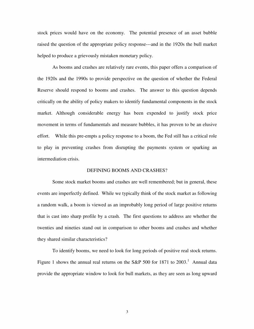
Figure 4 graphs a measure of the equity premium and the stock yield. The stock

yield is based on the S&P500, while the risk free rate is composed of three series spliced

together: the 10 year constant maturity U.S. government bond rate for 1941-2003, high

grade industrial bonds for 1900-1940, and high grade railroad bonds for 1871-1899.9 The

estimated stock yield is equal to the dividend yield and the average growth of dividends.

The nominal and real rate of growth of dividends was 3.9% and 1.7%.10

After a long period of relatively constancy in the nineteenth century, the equity

premium rose to over 6% after World War I. During the 1920s, it declined back to its

8 They point out that at higher discount rates of 7% to 9% percent that were usually presumed to have prevailed, very high growth rates of 3.4% to 5% would have been required. 9 U.S. government constant maturity bonds yields are found on www.freelunch.com. The high grade industrials (series 13026) and McCaulay’s railroad bonds (series 13019a) were obtained from the NBER website. 10 The real rate is calculated using the consumer price index. Blanchard (1993) measures the equity premium where the growth of dividends is not fixed, however is very similar.

20

previously level, then during the boom fell to its lowest point yet. If measured on a

monthly basis, the equity premium hit an unprecedented 2% during the bull market of

1928-1929. The Great Depression elevated the premium to an historic high. By the

1960s, it returned to the nineteenth century level. The brief period where there appears to

be an equity discount is not the result of any decline in the dividend yield but of the

unexpected rise in interest rates in the early 1980s. However, since the late 1980s, the

equity premium appears to have collapsed.11

The perception that equities are less risky and hence the equity premium should

decline was a common explanation for the nineties boom. Among the most bullish of the

bulls were Glassman and Hassett whose book The Dow 36,000 (1999) proclaimed a

“paradigm shift”:

Stocks should be priced two to four times higher---today. But it is impossible to predict how long it will take for the market to recognize that Dow 36,000 is perfectly reasonable. It could take ten years or ten weeks. Our own guess is somewhere between three and five years, which means that returns will continue to average about 25 percent per year. (p.13)

Their optimism was predicated on equation 2, assuming a real long term bond rate of 2%

and a 2.3% real growth rate of dividends, permitting a dividend yield of 1.5% to fall to

0.5% with a tripling of stock prices.12 Glassman and Hassett argued that a diversified

portfolio of stocks was no more risky than an investment in U.S. government bonds.

Once investors fully appreciated this fact, the equity premium would vanish as stock

prices were bid up. To support their argument, they pointed to the fact that transactions

costs had been greatly lowered by mutual funds, 401(k) plans, internet trading,

11 The disappearance of a substantial equity premium seems to bear out Mehra and Prescott’s (1985) claim that at reasonable levels of risk aversion, it is not possible to justify risk premium any larger than 0.25 percent in the absence of market imperfections.

21

computerization and other innovations that permitted investors to more easily acquire

information to diversify their portfolios.

The same factors---increased participation and diversification---that have been

used to explain the recent decline in the equity premium were also present in the 1920s.

Traditionally, investing in the stock market was restricted to the well-to-do but the wider

public entered the market in the 1920s. Smaller investors were brought into the market as

innovations made it easier for them to diversify their portfolios. One important

development was the expansion of the investment trusts---precursors to today’s mutual

funds, which grew from 40 in 1921 to 750 in 1929. After the stock market collapse of

1929 and the prolonged depression, the market was deserted by the small investors who

returned only slowly. By the end of the twentieth century, mutual funds facilitated the re-

emergence of small investors. Between 1990 and 2002, the number of these funds

climbed from 2,338 to 7,267 and the number of accounts and net assets rose from 61

million with $1,065 billion to 251 million with $6,392 billion.13

An increase in the stock market participation rate could decrease the required risk

premium on stocks because it would spread market risk over more of the population. The

Survey of Consumer Finances showed that the number of shareholders in the U.S. rose

from 52.3 million in 1989 to 69.3 million in 1995, with people entering the market at

younger ages (Heaton and Lucas, 1999). In addition, stockholders seem to be more

diversified, which would allow holders to demand a lower rate of return. Whereas, few

very investors had more than ten stocks in the 1960s, (Friend and Blume, 1978), the

potential for diversification has increased by mutual fund ownership, yet risk tolerance

12 Glassman and Hassett, p. 72-73. 13 Investment Company Institute (2003).

22

seems only to have increased slightly from 1989 to 1995. Heaton and Lucas (1999)

suggest that individuals who already own stocks are more risk-tolerant than those who do

not, implying that the addition of new stockholders might lower the average level of risk

tolerance, reducing the effect of wide ownership on the equity premium.

To examine the effects of increased participation and diversification, Heaton and

Lucas (1999) calibrated an overlapping generations model where only some households

hold equity and there is aggregate and idiosyncratic income risk. They found that

substantial changes in participation rates have only a small effect on the equity premium.

Diversification is more potent, but this factor has not increased as much as popularly

perceived. Mutual funds may have mushroomed, but as late as 1995 only 16.5% of

equity was owned through mutual funds. Furthermore, households that held stock had

almost half invested in their employing company (Vissing-Jorgensen, 1999). Thus,

increased participation and diversification may only explain a limited part of the

downward trend in the equity premium.

The sharp decline in the equity premium may also be explained by the inflation.

Using independent measures of equity risk from cross sectional data, Campbell and

Vuolteenaho (2004) found inflation explained half of the movement in the dividend yield.

The falling dividend yield of the late 1920s was attributable to a drop in risk. The

increase in the dividend yield in the 1930s and 1940s was dominated by the increase in

risk, which overwhelmed the effect of deflation that would have lifted prices. The

declining dividend yield of the 1950s and early 1960s was moved primarily by the falling

measures of equity risk. But rising inflation from the late 1960s through the 1970s raised

the dividend yield. By the late 1980s and 1990s, it was falling again, this time because

23

both risk and inflation were declining. Campbell and Vuolteenhao contend that higher

inflation was not correlated with any subjective measure of risk that would imply rational

pricing. Instead inflation increased expected long-term real dividend growth because

investors formed subjective growth forecasts by extrapolating past nominal growth rates

without taking inflation into consideration. The result was that stocks tended to be

overpriced when inflation was low and underpriced when inflation was high. They

blamed this “mis-pricing” of stocks by the persistent use of the “Fed model” by many

contemporary investment professionals who counseled investors to compare the yield on

stocks (the dividend yield) with the yield on Treasury bonds plus a risk factor. Use of

this model produces some inflation illusion.14 They concluded that at the end of 1999,

when dividend growth and the risk measures justified a dividend price ratio of 3.3, it was

observed to be 1.2.

While a huge effort has been expended by financial economists to explain the

movement of stock prices in terms of fundamentals, it has had a very limited success.

Changes in earnings growth and the discount rate cannot fully account for the buoyant

markets of the 1920s and 1990s. As Campbell (1999) bleakly explained: “The recent

run-up in stock prices is so extreme relative to fundamental determinants such as

corporate earnings, stock-market participation, and macroeconomic performance that it

will be very hard to explain using a model fit to earlier historical data.”

If there were bubbles in 1929 and 1999, they would have distorted consumption and

investment. A boom in stock prices would raise household wealth helping to drive

consumption, and new investment would look more attractive because soaring stock

prices would raise market value to book value in Tobin’s q. In addition, the improvement

14See also Campbell and Cochrane (1999)..

24

in the value of collateral would have allowed more firms to borrow. Firms might also

switch to equity finance from debt finance because of a lower equity premium. Rising

stock prices by increasing investment would have driven up the observed real growth

rate, making the apparent productive capacity of the economy greater. If stock prices do

not reflect fundamentals, some investments should not have been undertaken because

they did not really have had positive internal rates of return. The result will be

overinvestment and unusable capacity. Romer (1990) compared the behavior of

consumer spending and stock market wealth for the crashes of 1929 and 1987. She found

that the relationship between stock price variability and consumer spending were similar

for both periods, although the continued high level of volatility after 1929 was greater. In

the boom and bust, wealth had its strongest effect on consumer durables, raising

purchases during the bull market then drastically reducing consumption after the crash.

Eichengreen and Mitchener (2003) estimated an investment equation, where the doubling

of Tobin’s q that occurred between 1926 and 1929, produced an 18% increase in

investment and the collapse afterwards yielded a greater effect.

If fundamentals drive the market then there is no unwarranted consumption or

investment. Yet, studies of fundamentals cast doubt on whether stock market booms are

entirely attributable to fundamentals, suggesting that if one could measure the deviations

from fundamentals, there would be a role for incorporating asset prices or some measure

of asset mis-pricing into the Federal Reserve’s decision-making.

25

WHAT IS THE OPTIMAL POLICY?

If a consensus had been reached in macroeconomics at the end of the twentieth

century, it was that monetary policy should have as its primary goals price stability and

growth with no significant role for asset prices. Thus, Alan Greenspan’s 1996 warning

that the market was possessed with an “irrational exuberance” astonished many schooled

in the history of the Federal Reserve. It had been long been held as an article of faith that

the Fed had erred critically in 1929 when it focused on the buoyant stock market. Tight

policy, partly induced by its concern for the market, is generally viewed as having made a

mild recession worse, initiating the Great Depression of the 1930s. Greenspan’s

jawboning was eerily reminiscent of the Federal Reserve Board’s policy in early 1929

and opened a debate on whether monetary policy should respond to asset markets.

The question whether the central bank should respond to asset booms and busts is

relatively new. The current standard framework for policy is inflation-targeting

(Bernanke and Mishkin, 1997). Publicly announced medium-term inflation targets are

used to set a nominal anchor for monetary policy, allowing the central bank limited

flexibility to stabilize the real economy in the short-run. In a small calibrated

macroeconomic model, Bernanke and Gertler (2000, 2001) found that an inflation-

targeting rule stabilizes inflation and output when asset prices are volatile, driven either

by a bubble or technology shock. They concluded that there was no additional gain from

responding directly to asset prices because although a response to stock prices can lower

the variability of the output gap, it may increase the variability of inflation. Additionally,

they believe is that it is more difficult to identify the fundamental component of stock

26

prices than it is the output gap. In their view, any attempt to address asset volatility runs

the risk of imparting instability to prices and output, especially if measurement of

fundamentals is flawed.

Yet, some have argued that asset prices ought to be directly incorporated into

inflation targeting Cecchetti, Genberg, Lipsky, and Wadhwani (2000) proposed that a

central bank should adjust monetary policy not only in response to forecasts of future

inflation and the output gap but also to asset prices, developing procedures to identify

asset price “misalignments.” They believed that it is no more difficult to measure stock

price misalignments than it is the output gap or the equilibrium value of the real interest

rate.15 Cecchetti et. al. estimated the warranted risk premium in 2000 to be 4.3%, which

would have justified a S&P500 level less than half of the observed level. Their model

suggested that by 1997, the Federal Funds rate should have been 10.35% as opposed to

the actual 5.51%. This rate would have kept inflation at under 3%, with a small output

gap and a risk premium of just under 3%.

Bordo and Jeanne (2002) also make a case for pre-emptive monetary policy with

a Taylor rule model where productivity shocks can cause large price reversals. Boom-

bust episodes are identified with a simple filter where the three year growth of real stock

prices exceeds a critical value. They are concerned that during a boom, rising stock prices

raise the price of collateral, inducing firms to borrow; while a bust creates financial

instability by quickly lowering the value of collateral, yielding a collateral-induced credit

crunch. In their view, a central bank should carry out monetary policy in terms of

insurance, trading off the loss in output and price stability against the probability of a

27

costly credit crunch and a fall in real output. Bordo and Jeanne found that such a policy,

responding to a bull market, sometimes dominates a simpler Taylor rule in its sacrifice of

current output against the risk of a credit crunch.

This literature is new and growing, though the consensus remains that the Fed

should not incorporate asset prices directly into its policy considerations. While an

optimal policy rule may or may not include intervention in response to asset prices, the

Fed has been accused of incorrectly responding to the booms of the 1920s and 1990s.

THE ROLE OF THE FEDERAL RESERVE

How did policy makers in the twenties and nineties confront the booming

markets? Did their policies hinder or aggravate the booms? These issues were part of the

debates of both decades.

The bull market of the twenties had its origins in the long post-World War I

economic boom. Immediately after the high wartime inflation, the economy experienced

a boom and hard recession. It was a wrenching experience for financial intermediaries,

with numerous bank failures. But, the economy quickly stabilized and began to grow

rapidly, with two brief contractions in 1923-1924 and 1926-1927. Overall, between 1922

and 1929, GNP grew at a rate of 4.7% and unemployment averaged 3.7%. Anchored by

the gold standard, prices varied but there was no trend inflation.16 The end of the war

freed the Federal Reserve from its obligation to assist the Treasury’s financing of the war;

and the government balanced its budget, cutting expenditures and taxes. Once released

15 Bernanke and Gertler (2001) are highly critical of Cecchetti and argue his policy rule requires that the central bank know that the boom is driven by no-fundamentals and the exact time when the bubble will burst. 16 Historical Statistics, p. 135 and 226.

28

from keeping interest rates artificially low, the Fed accommodated seasonal demands for

credit and the close coincidence in the timing of the actions of the Fed and the turns in the

business cycle, imply that it helped to smooth economic fluctuations.

Some argued that the initial stock market boom of 1928-1929 was fueled by

expansionary monetary policy driven by international considerations. Having returned to

gold at an over-valued prewar parity, Britain was suffering from high unemployment and

a balance of trade deficit. In the spring of 1927, Germany raised interest rates

intensifying the pressure on the British balance of payments. At the same time, the Bank

of France attempted to halt the appreciation of the franc by selling francs for sterling,

which it then attempted to covert into gold at the Bank of England. When at a scret

Long Island conference in July 1927, the Reichsbank and the Bank of France offered

only minor concessions to address this threat to the newly restored gold standard, the Fed

took the lead and eased monetary policy. Further influenced by the slowdown in the U.S.

economy, the Fed cut the discount rate and purchased securities. But the minutes of the

Open Market Investment Committee make it clear that the majority worried about how

the stock market would react to this policy. One Board member, Edmund Platt spouted:

“Lower [the discount rate] in New York first and to hell with the stock market.” (quoted

in Clarke, 1967, p. 127).

While this shift in Fed policy was unexpected, it is difficult to see how it could

have had a big impact on the stock market. The interest cut was small and brief, as a

contractionary policy was initiated in January 1928 with the discount rate ascending from

3 ½ to 5 percent by August 1928. In addition, there were heavy open market sales.

Although the discount rate remained unchanged for another year, monetary policy has

29

been characterized generally as tight for the remainder of stock market boom. In 1928

and 1929, high-powered money and the consumer price index fell and M1 grew only

slightly in 1929. In spite of this evidence, many, including Strong felt that this tightening

was begun too late, to halt the advance of the stock market (Clarke, 1967).

Although concerned about protecting international gold reserves, the Federal

Reserve was obsessed with the stock market and what it regarded as the excessive

expansion of credit for speculation. Following the “real bills doctrine,” the founders of

the Fed had hoped that the bank’s discounting activities would channel credit away from

“speculative” and towards “productive” activities. Even in the early 1920s, many

members of the Board and banks were frustrated by the amount of credit that the stock

market seemed to absorb and looked for some way to reduce the volume of brokers’

loans. Almost all Fed officials agreed about this issue but they were split over the

appropriate policy; and policy inaction, after the August 1928 increase in the discount

rate, reflected an intense struggle.

The Federal Reserve Board believed that “direct pressure” or jawboning could be

used to channel credit away from speculation. The Board also wanted the Federal

Reserve banks to deny access to the discount window to member banks making loans on

securities. In February 1929, the chairman Roy Young spoke out against speculation and

issued a letter to all Federal Reserve banks, instructing them to limit "speculative loans."

Brokers' loans by member banks did not increase after this date, but the market was supplied

instead by non-member banks, corporations and foreigners. In contrast, the Federal Reserve

Bank of New York contended that it could not refuse to discount eligible assets and that it

was impossible to control credit selectively. It argued that speculation could only be

30

reduced by raising the discount rate. The Board was not persuaded. Between February

and August 1929, it refused New York’s eleven requests to raise the discount rate

(Friedman and Schwartz, 1963). According to Clarke (1967, p. 155), the New York Fed

believed that if the Fed could break the boom early, the adverse effects on the U.S. would

be small compared to the “disastrous consequences for both the domestic and

international economies that would result from a prolongation of speculative excesses

and from the inevitable and violent collapse of the speculative bubble.” Only in August

1929, did the New York Fed finally prevail. Unfortunately, the discount rate was raised

from 5 to 6% just as the economy was reaching its cyclical peak.

The market, declining since early September, collapsed on Black Thursday,

October 24, and Black Tuesday, October 29. Margin calls and distress sales of stock

prompted a further plunge; while lenders withdrew their loans to brokers, threatening a

general disintermediation. The New York Fed promptly encouraged the New York City

banks to increase their loans to brokers, made open market purchases, and let its member

banks know that they could freely borrow at the discount window. The direct effects of

the crash were thus confined to the stock market. The Fed’s prompt action ensured that

there were no panic increases in money market rates and no threat to the banks from

defaults on brokers’ loans. While the New Fed’s response has been recognized in

hindsight as the correct response, the Board disapproved and censured the New York

Fed. In spite of the recession, the Board maintained its tight monetary policy,

aggravating the economy’s slide and provoking a further decline in the market. The fall

in the stock market, by reducing household wealth and the value of collateral added to the

monetary shock that stunned the economy (Friedman and Schwartz, 1963).

31

The Fed’s experience in the 1920s raises three policy questions. The first is

whether the Fed’s looser policy in 1927 exacerbated the boom at a time when it could

have been restrained. Board member Adolph Miller and many critics after the crash

blamed the New York Fed for permitting an excessive credit expansion (Meltzer, 2003).

Some modern students, including Eichengreen (1992), have concluded that the Fed erred

in loosening its policy, it is difficult to find a plausible reason for a tighter policy.

Although contemporaries worried about speculative excess in the market, mid-1927

precedes the conventional date of the boom’s beginning---early 1928. In fact, monetary

growth for the year was quite modest, at a little over 1% (Meltzer, 2003), and the

economy had hit its peak in October 1926. Most contemporary indicators suggested to the

Fed that policy should be eased not tightened; the same holds true for a Taylor rule; and

Bordo and Jeanne’s (2002) measure of excessive asset growth does not identify a boom

in mid-1927. Finally an augmented Taylor rule (Cecchetti, 2000) does not recommend a

policy change as the equity premium for 1927 was near its historic average.

The second policy question is how the Fed should have reacted to the crash. New

York’s prompt intervention in 1929 to prevent the shock spreading to the rest of the

financial system is regarded as a canonically correct response (Friedman and Schwartz,

1963). The third policy question is whether the Fed focused too much on the stock

market boom after 1928, ignoring the fact that the economy was entering a recession.

The scholarly consensus here is that policy was excessively preoccupied with speculation

after the crash, inducing the Fed to continue a restrictive policy long after the economy

was in a steep decline.

32

The lessons learned from the experience of the 1920s have strongly conditioned

central bankers’ responses to subsequent crashes. Like 1929, the financial system in 1987

came under enormous stress as brokers needed to extend a huge amount of credit to their

customers who were hit by margin calls. Specialists and traders in stock index futures

also found it difficult to obtain credit. Fearful that there would be a collapse of securities

firms, with ramifications for the clearing and settlements system, the Open Market desk

increased bank reserves by 25% and the Fed pushed commercial banks to supply broker-

dealers and others with credit. While interest rate spreads widened at the beginning of

the crisis, they quickly diminished. Finally the Fed withdrew most of the high-powered

money that it had provided as the crisis subsided. In contrast, the slower collapse of the

1990s market produced no calls for intervention as intermediation and the payments

system were not threatened. In general, the conclusion that the Fed was mistaken to

focus on the stock market after the 1929 crash has convinced most central bankers to take

a position of “benign neglect” vis-à-vis asset bubbles.

Thus, it is primarily the first question---should a central bank intervene in an asset

price boom---that still appears to be open. A comparison of the 1990s with the 1920s is

consequently useful, as there appear to be strong parallels in economic developments and

policy debates. Like the 1920s, the 1990s saw a long period of rapid growth after a

period of severe disruptions. The unanticipated inflation of the 1970s and the Fed’s

decision to wring out inflation in 1979 contributed to a wave of bank and saving and loan

failures, cresting in the mid-1980s. By the beginning of the new decade, banks had

increased their capital accounts and strengthened their balance sheets. After a sharp

recession in 1990-1991, the economy experienced its longest expansion on record from

33

March 1999 to March 2001. Real gross domestic product grew at 3.3% and

unemployment averaged 5.5%. In many respects, the nineties was the most stable post-

World War II decade (Mankiw, 2003).

In 1993, the chairman of the Federal Reserve Board, Alan Greenspan announced

that the Fed would pay less attention to monetary aggregates than it had in the past, as

their behavior did not appear to give a very reliable policy guide. The Fed shifted to

interest rate targeting, and in particular the Federal funds rate. Most observers believe

that the Fed followed some approximation to a Taylor rule, focusing on inflation and

growth and leaving other issues that inflamed public debate, including fiscal policy,

“irrational exuberance,” and international financial crises, to negligible roles (Mankiw,

2003). One of the few exceptions to this consensus is Cecchetti (2003) who claimed that

as equity prices boomed, the FOMC adjusted its interest rate targets. Examining the

FOMC minutes and transcripts from 1981 to 1997, he measured the relative occurrence

of references to the securities markets and found that it rose just as the equity premium

was falling. Estimating an augmented Taylor rule with additional variables---the equity

premium for the presence of a bubble and a measure of banking system leverage for

financial distress---he found that the FOMC adjusted interest rates to changes in the

equity premium.17

Whether or not the Fed factored the stock market into its policy, independent of

inflation and growth objectives, it boldly voiced concerns about the behavior of the

market. Well before the IT-Nasdaq boom, the bull market raised alarms at the Fed, just as

it had in 1927-1928. While the price-earnings ratio was increasing, all measures of

17 If true, this behavior would represent a major change in policy, though the equity premium may be a proxy for aspects of inflation and output growth not captured by the variables in a standard Taylor rule.

34

productivity growth in the early 1990s showed little reason for expecting a future surge in

earnings and dividends. In 1996, Federal Reserve Board Chairman Alan Greenspan

castigated the stock market as exhibiting “irrational exuberance.” Yet, this jaw-boning,

seeming to mimic the actions of early 1929, was not followed by any effort to tame the

market. The lesson of the 1920s’ intervention may have may have restrained the Fed,

and the it certainly would have been wary about trying to deflate one group of stocks in

the technology sector without affecting the whole market. The verbal berating of the

market diminished later in the decade when evidence of a productivity upsurge gave the

Fed less cause to fear that its low interest rate policy would lead to inflation.

In an economy of higher growth in the late 1990s, the Fed’s policy has been

characterized as one of “forbearance” (Blinder, 2002). However, the Fed did not hesitate

when inflationary pressures appeared. Between February 1994 and February 1995, it

raised interest rates 3%, after a rapid expansion following the 1990-1991 recession,

securing a recession-less “soft landing.” Afterwards, policy was largely neutral until the

September 1998 collapse of Long-Term Capital Management (LTCM), a $100 billion

hedge fund, which followed the Asian crisis. Fearing its demise would panic financial

markets, the Fed strong-armed the leading New York banks to assist with an orderly

liquidation and cut the Fed funds rate three times. Some critics have asserted that this

action left policy too loose and allowed the boom in the stock market to take off in its

final phase. They have argued that it was too late when the Fed finally began to raise

interest rates in June 1999. Yet, the decline of less than 100 basis points in the Fed funds

rate and the 10 year bond rate were not seen at the time as wildly inflaming the boom.

Measured by all three indices in Figure 2, the market had retreated in August 1998 and

35

was largely flat until December 1998-January 1999 when it resumed its ascent; and there

was no signal from the dividend yield or price-earnings ratios. Like the loosening of

policy in 1927, this action came at a time when the market was quiescent. Given the

similar rise in the market when policy was neutral, this action may have been a minor

fillip at best.

CONCLUSION

This survey of fundamentals-based equity valuations reveals the enormous

difficulty of identifying fundamentals in forward looking assets. At the same time, little

evidence can be mustered to support Shiller’s (2000) assertion that the markets are almost

exclusively driven by waves of optimism or pessimism. Estimates that apportion the

degree to which bubbles determine asset prices relative to fundamentals are at best

fragile. Perhaps, it is not surprising that “benign neglect” is typically the accepted policy

by both those who favor fundamental and bubble explanations.

The Fed has been blamed for contributing to stock market booms. Two

instances—in 1927 when the Fed helped Britain stay on the gold standard and in 1998

when the Fed responded to the collapse of LTCM—are sometimes used to argue that the

Fed should have pursued a tighter policy earlier. However, it is hard to regard these

relatively modest stimuli as central to an explanation of the subsequently soaring

markets. Furthermore, this criticism has a 20-20 hindsight quality, as measures of a

bubble that should have alerted policy only appeared later in 1928 and 1999.

Fortunately, the Fed in the 1990s was not fixated on speculative credit, as was the

Fed of the 1920s and 1930s, saving it from dangerous deviations from the appropriate

36

policy targets of price stability and full employment. The Fed has a limited but vital role

in responding to stock market crashes. When the abruptness of the crash threatens the

payments system and intermediation, a classic lender of last resort is appropriate as

occurred in 1929 and 1987. In addition, even if the market’s descent is slower and the

financial system has weak balance sheets, intervention may be appropriate to prevent a

broader financial crisis. But in both cases, it is a brief intervention that is required, not a

shift in the Fed’s intermediate or longer-term goals.

37

Bibliography Bernanke, Ben S. and Mark Gertler, “Monetary Policy and Asset Price Volatility,” (NBER Working Paper 7559, February 2000). Bernanke, Ben S. and Mark Gertler, “Should Central Banks Respond to Movements in Asset Prices?” American Economic Review 91:2 (May 2001), pp. 253-257. Bernanke, Ben S. and Frederic Mishkin, “Inflation Targeting: A New Framework for Monetary Policy,” Journal of Economic Perspectives 11:2 (Spring 1997), pp. 97-116. Blanchard, Olivier J. and Mark W. Watson, “Bubbles, Rational Expectations and Financial Markets,” in Paul Wachtel, ed., Crises in the Economic and Financial Structure (Lexington: D.C. Heath and Company, 1982), pp. 295-315. Blanchard, Olivier, J., “Movements in the Equity Premium,” in William C. Brainard and George L. Perry, eds., Brookings Papers on Economic Activity 2 (Brookings Institution: Washington, D.C., 1993), pp. 75-138. Blinder, Alan, “Comments,” in “U.S. Monetary Policy During the 1990s,” in Jeffrey A. Frankel and Peter R. Orszag, American Economic Policy in the 1990s (Cambridge: MIT Press, 2002), pp. 44-51. Blume, Marshall and Irwin Friend, Irwin, The Changing Role of the Individual Investor (New York: Wiley, 1978). Bordo, Michael and Olivier Jeanne, “Boom-Busts in Asset Prices, Economic Instability, and Monetary Policy,” (NBER Working Paper 8966, June 2002). Campbell, John Y. and Robert J. Shiller, “Stock prices, earnings, and expected dividends, Journal of Finance 43 (1988), pp. 661-676. Campbell, John Y., “Comment,” in Ben S. Bernanke and Julio S. Rotemberg, eds., NBER Macroeconomics Annual (Cambridge: MIT Press, 1999), pp. 253-262. Campbell John Y. and Tuomo Vuolteenaho, “Inflation Illusion and Stock Prices,” (NBER Working Paper 10263, January 2004). Cecchetti, Stephen G, Hans Genberg, John Lipsky and Shushil Wadhwani, Asset Prices and Central Bank Policy (Geneva Reports on the World Economy 2: ICBM and CEPR, 2000). Cecchetti, Stephen G., “What the FOMC Says and Does When the Stock Market Booms,” (mimeo August 2003). Chandler, Alfred D., The Visible Hand: The Managerial Revolution in American Business (Cambridge: Belknap Press, 1977).

38

Clarke, Stephen V.O., Central Bank Cooperation, 1924-1931 (New York: Federal Reserve Bank, 1967). Cochrane, John H., “Volatility tests and efficient markets: A review essay,” Journal of Monetary Economics 27 (1991). De Long, J. Bradford, Andrei Shleifer, Lawrence H. Summers and Robert J. Waldmann, “Noise Trader Risk in Financial Markets,” Journal of Political Economy 98, 4 (August 1990), pp. 703-738. Dice, Charles Amos, New Levels in the Stock Market (1929) Donaldson, R. Glen and Mark Kamstra, “A New Dividend Forecasting Procedure That Rejects Bubbles in Asset Prices: The Case of 1929’s Stock Crash,” Review of Financial Studies 9:2 (Summer 1996), pp. 333-383. Eichengreen, Barry, Golden Fetters: The Gold Standard and the Great Depression, 1919-1939 (Oxford: Oxford University Press, 1992). Eichengreen, Barry and Kris Michener, “The Great Depression as a credit boom gone wrong,” (Bank for International Settlements, Working Paper No. 137, September, 2003). Fama, Eugene F, and Kenneth R. French, “Dividend yields and expected stock returns,” Journal of Financial Economics 22 (1988), pp. 3-25. Fisher, Irving, The Stock Market Crash—And After (1930) Fisher, Lawrence, “Some New Stock Market Indexes,” Journal of Business 39, 1 Part 2 Supplement (1966), pp. 191-225. Flavin, Majorie A, “Excess Volatility in the Financial Markets: A Reassessment of the Empirical Evidence,” Journal of Political Economy 91 (December 1983), pp. 929-89. Flood, Robert P. and Robert J. Hodrick, “On Testing for Speculative Bubbles,” Journal of Economic Perspectives 4, 2 (Spring 1990), 85-101. Friedman, Milton and Anna J. Schwartz, A Monetary History of the United States, 1867-1960 (Princeton: Princeton University Press, 1963). Freelunch. www.freelunch.com Glassman, James, and Kevin Hassett, The Dow 36,000: The New Strategy for Profiting from the Coming Rise in the Stock Market (New York: Times Business, 1999).

39

Gordon, Robert J., “Interpreting the ‘One Big Wave’ in U.S. Long-Term Productivity Growth,” (NBER Working Paper 7752, June 2000). Gordon, Robert J., “Does the ‘New Economy’ Measure up to the Great Inventions of the Past?” (NBER Working Paper 7833, August 2000). Heaton, John and Deborah Lucas, “Stock Prices and Fundamentals,” in Ben S. Bernanke and Julio S. Rotemberg, eds., NBER Macroeconomics Annual (Cambridge: MIT Press, 1999), pp. 213-242. Investment Company Institute, Mutual Fund Fact Book 43rd edition (2003). Jovanovic, Boyan and Peter L. Rousseau, “Moore’s Law and Learning-By-Doing,” (NBER Working Paper 8762, February 2002). Keynes, John Maynard, The General Theory of Employment, Interest and Money (Macmillan, 1936). Kleidon, Allan W., “Variance Bounds Tests and Stock Price Valuation Models,” Journal of Political Economy 94:5 (1986), pp. 953-1001. Lamont, Owen, “Earnings and Expected Returns,” Journal of Finance 53:5 (October 1998) pp. 563-1587. Mankiw, N. Gregory, “U.S. Monetary Policy During the 1990s,” in Jeffrey A. Frankel and Peter R. Orszag, American Economic Policy in the 1990s (Cambridge: MIT Press, 2002), pp. 19-43. Mehra, Rajnish, and Edward C. Prescott, “The Equity Premium: A Puzzle,” Journal of Monetary Economics 15 (March 1985), pp. 145-61. Meltzer, Allan H., A History of the Federal Reserve Vol. I (Chicago: University of Chicago Press, 2003). Mishkin, Frederic S. and Eugene N. White, “U.S. Stock Market Crashes and Their Aftermath: Implications for Monetary Policy,” in William C. Hunter, George G. Kaufman and Michael Pomerleano, Asset Price Bubbles: The Implications for Monetary, Regulatory, and International Policies (Cambridge, MIT Press, 2003), pp. 53-79.. Nordhaus, William D., “Productivity Growth and the New Economy,” Brookings Papers on Economic Activity 2 (2002), pp. 211-244. Patterson, Robert T., The Great Boom and Panic, 1921-1929 (Chicago: Henry Regnery Company, 1965).

40

Rappoport, Peter and Eugene N. White, “Was There a Bubble in the 1929 Stock Market?” Journal of Economic History 53:3 (September 1993), pp. 549-574. Rappoport, Peter and Eugene N. White, “Was the Crash of 1929 Expected?” American Economic Review 84:1 (March 1994), pp. 271-281. Romer, Christina, “The Great Crash and the Onset of the Great Depression,” Quarterly Journal of Economics (August 1990), Vol. 105. No. 3, pp. 597-624. Shiller, Robert J., “Do Stock Prices Move Too Much to be Justified by Subsequent Changes in Dividends?” American Economic Growth 71:2 (June 1981), pp. 421-435. Shiller, Robert J., Market Volatility (Cambridge: MIT Press, 1991). Shiller, Robert J., Irrational Exuberance (Princeton: Princeton University Press, 2000). Shiller, Robert J., http://www.econ.yale.edu/~shiller/data.htm

Sirkin, Gerald, “The Stock Market of 1929 Revisited: A Note,” Business History Review 49:2 (Summer 1975), pp. 223-31. Vissing-Jorgensen, Annette, “Comment,” ,” in Ben S. Bernanke and Julio S. Rotemberg, eds., NBER Macroeconomics Annual (Cambridge: MIT Press, 1999), pp. 242-253. Wigmore, Barrie A., The Crash and Its Aftermath: A History of Securities Markets in the United States, 1929-1933 (Westport: Greenwood Press, 1985). Williams, John B., The Theory of Investment Value (Cambridge: Harvard University Press, 1938). West, Kenneth D., “Dividend Innovations and Stock Price Volatility, Econometrica Vol. 56, No. 1, (January 1988), pp. 37-61. U.S. Department of Commerce, Historical Statistics of the United States (Washington, D.C: U.S. Government Printing Office, 1976).

41

Figure 1Real S&P Returns 1871-2003

and Twentieth Century Crashes

-50

-40

-30

-20

-10

0

10

20

30

40

50

1872

1876

1880

1884

1888

1892

1896

1900

1904

1908

1912

1916

1920

1924

1928

1932

1936

1940

1944

1948

1952

1956

1960

1964

1968

1972

1976

1980

1984

1988

1992

1996

2000

19031907

19171920

1929

1930-33

1937 19461940

1969-70

1973-74

1987 19902000-01

Figure 2 Boom and Bust 1920-1933

0

20

40

60

80

100

120

1920 1921 1922 1923 1924 1925 1926 1927 1928 1929 1930 1931 1932 1933

Pea

ks =

100

Dow Jones Cowles Equally Weighted

42

Figure 3

Boom and Bust 1990-2003

0

20

40

60

80

100

120

1990 1991 1992 1993 1994 1995 1986 1997 1998 1999 2000 2001 2002 2003

Ser

ies

Pea

ks =

100

Dow Jones S&P500 Nasdaq

Figure 4Stock Yield and Equity Premium

1871-2003

-6

-4

-2

0

2

4

6

8

10

12

14

1871

1875

1879

1883

1887

1891

1895

1899

1903

1907

1911

1915

1919

1923

1927

1931

1935

1939

1943

1947

1951

1955

1959

1963

1967

1971

1975

1979

1983

1987

1991

1995

1999

2003

Per

cent

Equity Premium Stock Yield