NBER WORKING PAPER SERIES

ARE ALCOHOL EXCISE TAXES GOOD FOR US?SHORT AND LONG-TERM EFFECTS ON MORTALITY RATES

Philip J. CookJan OstermannFrank A. Sloan

Working Paper 11138http://www.nber.org/papers/w11138

NATIONAL BUREAU OF ECONOMIC RESEARCH1050 Massachusetts Avenue

Cambridge, MA 02138February 2005

The views expressed herein are those of the author(s) and do not necessarily reflect the views of the NationalBureau of Economic Research.

© 2005 by Philip J. Cook, Jan Ostermann, and Frank A. Sloan. All rights reserved. Short sections of text,not to exceed two paragraphs, may be quoted without explicit permission provided that full credit, including© notice, is given to the source.

Are Alcohol Excise Taxes Good For Us? Short and Long-Term Effects on Mortality RatesPhilip J. Cook, Jan Ostermann, and Frank A. SloanNBER Working Paper No. 11138February 2005JEL No. I12

ABSTRACT

Regression results from a 30-year panel of the state-level data indicate that changes in alcohol-excise

taxes cause a reduction in drinking and lower all-cause mortality in the short run. But those results

do not fully capture the long-term mortality effects of a permanent change in drinking levels. In

particular, since moderate drinking has a protective effect against heart disease in middle age, it is

possible that a reduction in per capita drinking will result in some people drinking "too little" and

dying sooner than they otherwise would. To explore that possibility, we simulate the effect of a one

percent reduction in drinking on all-cause mortality for the age group 35-69, using several alternative

assumptions about how the reduction is distributed across this population. We find that the long-term

mortality effect of a one percent reduction in drinking is essentially nil.

Philip J. CookTerry Sanford Institute of Public PolicyBox 90245Duke UniversityDurham, NC 27708and NBERpcook@duke.edu

Jan OstermannCenter for Health Policy, Law, and ManagementDuke UniversityDurham, NC 27708j.o@duke.edu

Frank A. SloanCenter for Health Policy ResearchDuke UniversityBox 90253Durham, NC 27708-1111and NBERfsloan@hpolicy.duke.edu

3

Numerous states have recently increased their cigarette taxes, partly with the goal

of reducing smoking and thereby improving health (Sloan & Trogdon 2004). Advocates

for raising alcohol taxes also cite the public health argument (Cook 1982; Cook 1988;

Grossman, et al. 1993; Cook & Moore 2002), but few states have elected to do so in the

last couple of years.1 While the explanation for this difference may have to do with the

difference in political influence of the two industries (Sloan & Trogdon 2004), there is

also an important difference in the nature of the public-health claims. For an adult to

have a drink occasionally is not a health risk and may even confer a health benefit

(Rehm, et al. 2003a). Hence an increase in tax penalizes healthy as well as unhealthy

drinking practices. On the other hand, smoking in any amount is detrimental to health.

Alcohol excise taxation increases prices and reduces per capita consumption

(Cook & Tauchen 1982; Ruhm 1995; Clements, Yang & Zheng 1997; Young &

Bielinska-Kwapisz 2003). In principle, a tax-induced reduction in per capita

consumption of alcohol may involve reductions in both the prevalence of alcohol abuse

and the prevalence of moderate drinking, with opposite effects on mortality rates. The

net effect on mortality could be either positive or negative, and has not been established

empirically.

Some specific mechanisms by which drinking creates health risks and benefits are

well documented. For all age groups, drinking bouts sometimes lead to death from

overdose, or from injury resulting from accident or intentional violence (Cook & Moore

1993c; Birckmayer & Hemenway 1999; Hingson & Winter 2003). Chronic heavy

drinking may cause death due to organ damage, including liver cirrhosis (Rehm, et al.

2003a). On the other hand, it appears to be true that chronic drinking confers some health

benefits on middle-aged and older people. In particular, alcohol acts as an anti-

cholesterol drug, and epidemiological evidence suggests that moderate drinking is

associated with reduced mortality from heart disease and stroke (Corrao, et al. 2000).

1 Two states increased alcohol taxes in 2002, and six states in 2003 (http://www.cspinet.org/booze/taxguide/2003TaxMap.htm, accessed on December 20, 2004).

4

Thus an increase in alcohol excise taxes may be expected to reduce mortality rates

to the extent that it induces a lower incidence of risky drinking and lower prevalence of

chronic heavy drinking. But if older people drink too little in response to higher prices,

then the result may be increased cardiovascular death rates.

In what follows, we begin by presenting estimates suggesting that the short-term

effect of increases in alcohol taxes is to reduce all-cause mortality rates. The cumulative

long-term effects may be qualitatively different, especially for middle-aged people, and

must be estimated indirectly. To estimate these long-term effects, we combine new

estimates of the effect of per capita alcohol consumption on drinking patterns, with a

summary estimate from the epidemiology literature of the relative risks associated with

different levels of drinking. We calculate that a permanent reduction of one percent in

alcohol consumption per capita (induced by a tax increase or some other mechanism)

would have little net effect on mortality in middle age, defined as the age range 35-69.

(Our sensitivity experiments suggest that the effect may be positive or negative but is

always close to zero.) Since there is no known health benefit from drinking for younger

people, and considerable risks, we conclude that the public-health case for increased

alcohol taxation is strong.

Acute Effects of Drinking and Alcohol Taxes on Mortality

We begin the analysis by estimating the short-term effects of alcohol consumption

on all-cause mortality using a panel of annual state-level data for the period 1970-2000.

The regression specifications include the best-available measure of alcohol consumption

(annual state-level sales per capita), or an index of the alcohol excise taxes that apply in

the state, or both the tax and the consumption measures. All regression specifications

include state and year fixed effects, and control for two measures of economic conditions:

income per capita, and the employment-population ratio. This method was first

employed by Cook and Tauchen (1982) to estimate the short-term population-level

effects of drinking on cirrhosis mortality, and since then has been used to analyze the

5

effects of drinking and alcohol availability on injury death rates.2 To our knowledge, this

method has not previously been applied to all-cause mortality.

The results of our panel regressions are reported in Table 1. In the first column,

we see that average drinking (measured by ethanol sales per capita) has a positive effect

on all-cause mortality, with an elasticity of about 0.23. This estimate is quite precise,

with robust standard error (with state clusters) of .075.

An alternative approach to determining the effect of drinking on all-cause

mortality is to analyze mortality as a function of short-term variations in excise tax rates.

The results are reduced-form estimates under the assumption that taxes are passed on to

consumers in the form of higher prices – an assumption that is supported by the evidence

(Young & Bielinska-Kwapisz 2002). A causal interpretation requires that after

accounting for economic conditions, state excise tax variation is exogenous relative to

mortality rates. Columns 2 and 3 report respectively the estimated effects of a

comprehensive state excise-tax index and of the state beer excise tax. The former is

computed by averaging tax rates across beer, wine, and liquor, weighted by the

percentage of ethanol from each, to produce an average rate per ounce of ethanol. Details

concerning construction of the tax index are provided in the appendix. Both tax measures

are significantly negatively associated with all-cause mortality rates, suggesting that the

short-term causal effect of a tax-induced reduction in drinking is to lower mortality rates.

It is also of interest to include both the tax rate and per capita consumption. If the

short-term effect of taxes on mortality is channeled entirely through per capita alcohol

consumption, and does not change drinking patterns in relevant ways, then the tax

variable should have a coefficient near zero. Columns 4 and 5 of Table 1 confirm that

that is indeed the case.

2 The analysis of annual state-level panel data has documented the effects of alcohol control and availability on highway fatality rates (Ruhm 1995; Saffer & Grossman 1987a; Saffer & Grossman 1987b; Chaloupka, Saffer & Grossman 1993; Sloan, et al. 1994; Ruhm 1995; Eisenberg 2003; Young & Bielinska-Kwapisz 2003b), suicide (Sloan, et al. 1994; Markowitz, Chatterji & Kaestner 2003; Carpenter 2004b), and homicide (Cook & Moore 1993d; Sloan, et al. 1994). With the exception of homicide, the findings have been generally positive.

6

A further check on the results in Table 1 is to determine whether the estimates are

compatible with each other, given the effect of alcohol taxes on per capita ethanol

consumption. Table 2 reports the results of panel regressions on per capita sales of

ethanol, with specifications that mimic those in Table 1. Combining these results with

those from the mortality regressions in column 2 of Table 2, we see that a 1 cent per

ounce (1982-84 prices) increase in the tax index results in a 2.1 percent decrease in sales

per capita. This implies (from the elasticity estimate in Table 1, column 1) a 0.5%

reduction in all-cause mortality. That is reasonably close to the direct estimate of 0.7 %

(Table 1, column 2).

Mortality in middle age and later

The inclusion of “year” fixed effects in the panel regressions assures that national

trends are well accounted for. In this specification, the mortality effects are estimated

from year-to-year changes (in tax rate or sales), and hence are limited to estimating the

contemporaneous effect of drinking on mortality. While that may be an adequate

accounting for injury deaths, the cumulative effects of drinking careers on health are not

captured. The long-term cumulative effects of heavy drinking include numerous alcohol-

induced disorders of the gastrointestinal tract, most notably liver cirrhosis (Rehm, et al.

2003a; Yoon et al 2003}. But the long-term health consequences of drinking are not all

adverse. The main health benefits appear to be the prevention of coronary heart disease

and stroke (Klatsky, Friedman & Siegelaub 1974; Klatsky 2002; Corrao, et al. 2000;

Thun, et al. 1997; Marmot 2001; Britton & Marmot 2004). These and other

cardiovascular diseases are the leading causes of death in the United States, accounting

for nearly 40 percent of all deaths (over 900,000 people per year), so that even a

relatively small proportional reduction is noteworthy (Center for Disease Control and

Prevention 2004a). A further complication arises because even though drinking protects

against heart disease over the course of years, a single bout of heavy drinking may trigger

a heart attack (Britton & McKee 2000; Murray, et al. 2002) or lead to a fatal accident.

Hence the short-term mortality effects of an increase in drinking may be the opposite of

the long-term effects.

7

The risks and benefits of a drinking career are age-related. A meta-analysis of all-

cause mortality found that for men under age 45, death rates increase with alcohol

consumption on a near-linear basis (due to injury risks), but for middle-aged cohorts

follow a J-shaped curve (Rehm, Gutjahr & Gmel 2001): for those in middle age,

mortality rates are lower for those who drink moderately than for abstainers, but at some

point the mortality rate increases with alcohol consumption and eventually exceeds the

rate for abstainers (Britton & Marmot 2004; Murray, et al. 2002; Rehm, Greenfield &

Rogers 2001; White, Altmann & Nanchahal 2002). Over the entire age range, typical

estimates find a similar number of lives saved and lost from drinking in the United States

and Canada, but with an important difference – the victims tend to be quite young,

whereas it is older people whose lives are extended by drinking. If the calculation of

gains and losses is based on life-years gained and lost, or life years adjusted for disability,

then the losses greatly exceed the gains (Murray & Lopez 1997; Single, et al. 1999).

The implicit thought experiment underlying these estimates is to compare the

current mortality rate to a hypothetical rate associated with permanent population-wide

abstinence. What is missing from this literature is to consider the effect of a small long-

term reduction in per capita consumption of the sort that could be accomplished through a

modest change in the excise tax rate.

Our empirical approach is to chain together estimates of the all-cause relative

mortality risks from different levels of drinking, using estimates from a meta-analysis of

the literature with our own estimates of the effect of a change in middle-aged drinking

patterns of the sort associated with a small reduction in population-level alcohol

consumption. We begin with an analysis of drinking patterns as a function of per capita

consumption, and then estimate the associated mortality effects.

8

Drinking patterns.

State per capita sales data are generated from the tax-collection process and

presumably provide reasonably accurate estimates of consumption in most states.3

Consumption patterns, including the population prevalence of drinking, must be

estimated from self-report data on surveys. In what follows we use a recent survey, the

National Epidemiologic Survey on Alcohol and Related Conditions (NESARC),

conducted by National Institute on Alcohol Abuse and Alcoholism, fielded in 2001-2

with a representative sample of 43,093 non-institutionalized Americans age 18 and over

(National Institute on Alcohol Abuse and Alcoholism 2003). The NESARC-based

estimate of average consumption for the U.S. population captures only about half of

recorded sales nationwide, but in that respect is no worse than other such surveys.4

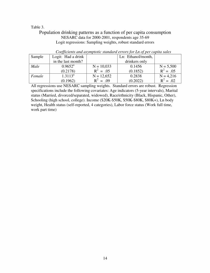
Table 3 presents logit-regression results indicating that the likelihood of a middle-

aged respondent reporting that he or she had at least one drink in the previous month is

closely related to per capita alcohol sales (in natural log form) in his or her state of

residence (after regression-adjusting for characteristics of the respondent). On the other

hand, the amount that drinkers report drinking appears to be only weakly related to per

capita sales, as suggested in Table 3 by the results of the ordinary-least-squares

regressions. Specifically, the elasticity of the odds of drinking with respect to per capita

sales is .97 for males and 1.31 for females (based on the logit results); the elasticity of

quantity consumed with respect to per capita sales is an insignificant .15 for males and

.28 for females. The suggestion in these results is that state-level factors (such as tax

rates) that change alcohol consumption do so primarily at the extensive margin. Thus a

reduction in per capita consumption is associated with an increase in the abstention rate,

but little change in the shape of the drinking distribution among drinkers. Since we do not

3 The main source of error stems from sales to out-of-state residents, which are proportionally large New Hampshire, Nevada, and a few other states where out-of-state travelers may account for a high proportion of the total sales. That source of error will be largely absorbed in the panel regressions by state fixed effects. 4 Based on NESARC data, the self-reported ethanol consumed in the past 12 months by respondents (who were age 18 and over) averaged 141.3 ounces. The NIAAA reports that the annual per capita sales in 2000 was 2.18 gallons of ethanol or 277.76 ounces total consumed by the population age 15 and older. Dividing the NESARC estimate by the NIAAA estimate gives the under-reporting estimate of 49 percent.

9

have complete confidence in these estimates, we perform a sensitivity analysis in what

follows.5

For the entire population there is an “adding up” constraint, requiring that the shift

in drinking patterns be compatible in the aggregate with changes in overall per capita

consumption. Strictly speaking this constraint does not apply to the samples under study

here (since per capita sales includes everyone, but our samples are limited to middle-age

people and distinguish between males and females). As it turns out the regression results

do nearly fit the adding-up condition for middle-aged females, but not males.

Mortality effects.

The curve relating all-cause mortality risk to drinking has been estimated in a

large number of epidemiological studies utilizing a variety of data sets. A recent meta-

analysis of the results for middle-aged populations (average age of 45 at baseline)

documents the J-curve for both males and females (Gmel, Gutjahr & Rehm 2003). The

summary statistics on relative risks after adjusting for other personal characteristics and

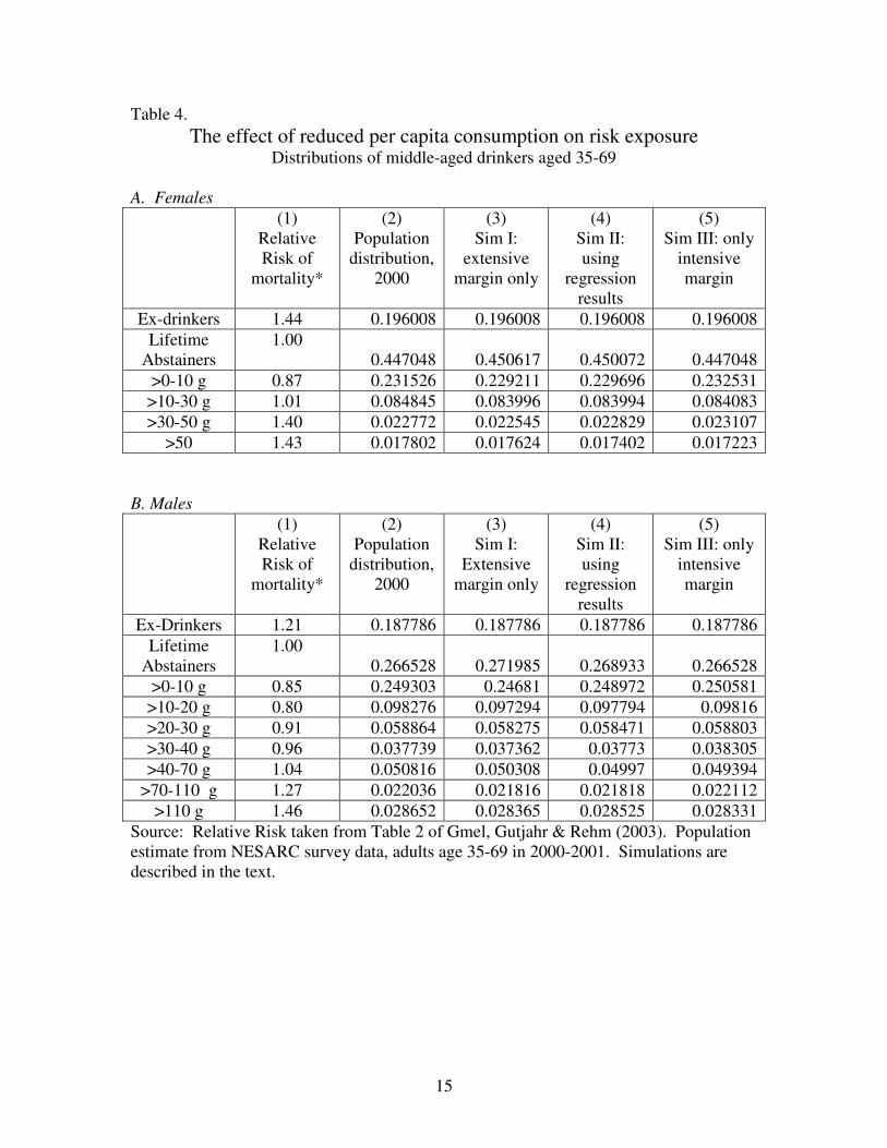
behaviors are given in Column 1 of Table 4. For females, the lowest relative risk is for

drinkers who consume no more than 10 grams of ethanol per day on average (less than

one standard drink, such as 12 ounces of beer or 4 ounces of wine). For males the lowest

relative risk occurs in the 10-20 gram range, which is about one standard drink per day.

It should be noted that these results are based on observational data and are

subject to a variety of problems of measurement and causal inference. Nonetheless they

represent the state of the art.6 We use the results to illustrate the calculations needed to

answer our question concerning the net effects on mortality.

5 It may strike some readers as more plausible that drinkers would respond to higher prices by cutting back rather than quitting entirely. We share that intuition. But it may be wrong: note that Cook and Moore (2001) found a similar pattern of results for youths. In any event, we conduct sensitivity tests as described below. 6 Drinking estimates are typically determined by a single questionnaire at the baseline of the study and are subject to reporting bias. These self-reports are typically interpreted as an indicator not only of current drinking but of a longer-term drinking habit. Self-selection bias with respect to the decision of whether and how much to drink has been a concern of this literature, but primarily focused on the “sick quitter” hypothesis, namely that some of those who currently abstain do so because they are sick and hence at

10

Using NESARC data, we tabulate the actual distribution of the middle-age

population across drinking categories (Column 2) and the distributions that, would have

resulted from a one percent reduction in per capita consumption under three different sets

of assumptions intended to bracket “reality” (Column 3-5).7 Simulation I assumes that

the effect of the tax increase and resulting one percent reduction in per capita

consumption is accomplished entirely at the extensive margin. One percent of the

drinkers become abstainers, and the distribution of drinkers over quantities is unaffected.

In other words, each category of drinking quantity loses one percent of its members.

Simulation III, on the other hand, assumes that there is no change at the extensive margin,

and that the reduction in per capita consumption is accomplished by a uniform downward

shift in consumption by drinkers. In effect, each drinker consumes 99 percent as much as

in reality. Simulation II adopts the intermediate assumption, generally guided by the

regression results, that the “action” occurs at both the extensive and intensive margin.

Specifically, we accept the point estimate from the NESARC logit regression as accurate,

and then use a percentage reduction in consumption by those who continue to drink that

is computed so as to result in a one percent reduction in overall consumption.8

We assume that the increase in abstainers in Simulations I and II occurs only in

the “lifetime” category, and not in the “previous drinker” category-- an important

assumption because the relative mortality risk is substantially higher in the latter. The

“previous drinker” category is likely to include a large group who quit because of health

problems (Gmel, Gutjahr & Rehm 2003). Since we are simulating the effect of an

increase in taxes, the proximate cause of the switch would (by assumption) be higher

prices rather than illness. The “lifetime abstainer” category seems better in capturing the

health effect.

greater risk of death. Indeed, quitters have higher death rates than lifetime abstainers (Gmel, Gutjahr & Rehm 2003). But other problems associated with self-selection have not been dealt with effectively. 7 Note that we are using self-report data on drinking to assign individuals to the various categories, despite the fact that such data are biased and error-prone. Our justification is that the epidemiological studies that generated the relative-risk estimates also employed self-report data. 8 The reductions are 0.56164% for males and 0.1541345% for females.

11

The first two simulations (where there is some movement from drinker to

abstainer) result in an increase in the population-weighted average in relative risk, while

the third results in a decrease.9 Table 5 summarizes the results translated into estimates

of deaths in a single year, together with the associated loss of life years. What is striking

about these results is that the numbers are small to the point of triviality in comparison

with the 700,000 annual deaths in this age group. Thus a permanent one-percent

reduction in drinking by the population age 35-69 would have a negligible effect on the

death rate. While it is not possible to say for sure whether the effect would be positive or

negative, fewer than 200 lives are at stake. Our best estimate (from Simulation II) is that

33 lives would be lost per year in middle age.

Assuming as noted that for younger individuals the relative mortality risk

increases monotonically with drinking, it is safe to say that the net effect for the entire

population of higher taxes is to reduce mortality rates.

In Sum

The direct evidence indicates that a tax increase resulting in a reduction in

drinking lowers all-cause mortality in the short run. The possibility that this effect would

eventually be reversed for middle-aged people (due to the cumulative effects of some

people drinking “too little” for a number of years) does not appear to be well founded.

For the age group 35-69, the long-term mortality effect of a one percent reduction in

drinking is essentially nil.

We make no attempt to estimate effects of a drinking reduction on disability and

morbidity, or on effects outside of the health arena (Manning, et al. 1991; Gmel & Rehm

2003).

9 For Sim 1, the increase is 31 and 74.5 millions for males and females respectively. For Sim 2 the corresponding numbers are 428.3 and 30.8. For Sim 3, the decline is 370.6 and 235.7 per million.

12

Table 1.

Effects of state ethanol sales/capita and alcohol excise taxes on all-cause mortality

Annual state panel data, 1970-2001* OLS regression results with fixed effects for state and year

Coefficients and Standard Errors (1) (2) (3) (4) (5) (6) Per Capita income (ln)

-.0115 (.0971)

.0653 (.1210)

.0086 (.1218)

.0343 (.0878)

-.0191 (.0893)

.0395 (.1195)

Employment-Population ratio (ln)

.0134 (.0883)

.204c (.108)

.180 (.112)

.0779 (.1044)

.0258 (.0971)

.193c (.110)

State alcohol sales per capita (ln)

.228a (.075)

.210b (.083)

.239a (.085)

Alcohol tax index -.0068c (.0039)

-.0019 (.0039)

-.0083c (.0040)

Beer tax -.0057b (.0028)

-.0006 (.0025)

Constant 5.793a (1.108)

6.453a (1.145)

6.964a (1.117)

5.464a (1.064)

5.804a (1.075)

6.066a (1.111)

State fixed effects? Yes Yes Yes Yes Yes Yes Year fixed effects? Yes Yes Yes Yes Yes Yes N 1,443 1,216 1,467 1,183 1,416 944 R2 .95 .95 .94 .95 .95 .95 Note: Robust standard errors in parentheses (state clusters). OLS regression specifications include year and state fixed effects. The regression sample includes all states that have tax data with the exception of specification (6) which is only for the 32 states and District of Columbia which have license systems. The alcohol tax index is in cents and is the combined tax rates of beer, wine, and liquor. The tax index uses state-specific weights (depending on average percentage of ethanol consumed in the form of beer, wine or liquor) multiplied by each tax to determine weighted rates, which are then summed. The beer tax is in cents per ounce of ethanol.

a=p<.01; b=p<.05 c=p<.10 *For specifications that only include taxes the data are for 1970 to 2001; for those with sales only the data are for 1970 to 2000; and for specifications with both taxes and sales the data re for 1971 to 2000.

13

Table 2. Elasticity of alcohol sales with respect to changes in tax

Annual State Panel data (1971-2000) OLS regression results with fixed effects for state and year

Coefficients and Standard Errors (1)

Beer Tax (state + federal, inflation

adjusted)

(2) Excise tax index (state + federal,

inflation adjusted)

(3) Excise tax index,

License states only

Per Capita income (ln) .197 (.180)

.188 (.208)

.133 (.214)

Employment-Population ratio (ln)

.543b (.212)

.643b (.244)

.604b (.268)

Alcohol tax index -.0211a (.0061)

-.0237a (.0068)

Beer tax -.0194a (.0045)

Constant 4.589b (1.764)

4.735b (2.059)

5.879b (2.231)

State fixed effects? Yes Yes Yes Year fixed effects? Yes Yes Yes N 1,416 1,183 912 R2 .94 .93 .93 Note: Robust standard errors in parentheses. OLS regression specifications included clustering at the state level along with year and state fixed effects. Regression sample for all states with beer tax or tax index values with the exception of specification (3) which is only for the states that have license systems (32 plus D.C.). The alcohol tax index is in cents and is the combined tax rates of beer, wine, and liquor. Tax index uses state-specific weights (depending on average percentage of ethanol from beer, wine and liquor) multiplied by each tax to determine weighted rates, which are then summed. Beer tax is in cents per ounce of ethanol.

a=p<.01; b=p<.05

14

Table 3. Population drinking patterns as a function of per capita consumption

NESARC data for 2000-2001, respondents age 35-69 Logit regressions: Sampling weights, robust standard errors

Coefficients and asymptotic standard errors for Ln of per capita sales Sample Logit: Had a drink

in the last month?

Ln: Ethanol/month, drinkers only

Male 0.9652a (0.2178)

N = 10,033 R2 = .05

0.1456 (0.1852)

N = 5,500 R2 = .05

Female 1.3113a (0.1962)

N = 12,652 R2 = .09

0.2838 (0.2022)

N = 4,216 R2 = .02

All regressions use NESARC sampling weights. Standard errors are robust. Regression specifications include the following covariates: Age indicators (5-year intervals), Marital status (Married, divorced/separated, widowed), Race/ethnicity (Black, Hispanic, Other), Schooling (high school, college). Income ($20K-$50K, $50K-$80K, $80K+), Ln body weight, Health status (self-reported, 4 categories), Labor force status (Work full time, work part time)

15

Table 4. The effect of reduced per capita consumption on risk exposure

Distributions of middle-aged drinkers aged 35-69 A. Females

(1) Relative Risk of

mortality*

(2) Population

distribution, 2000

(3) Sim I:

extensive margin only

(4) Sim II: using

regression results

(5) Sim III: only

intensive margin

Ex-drinkers 1.44 0.196008 0.196008 0.196008 0.196008 Lifetime

Abstainers 1.00

0.447048 0.450617 0.450072 0.447048 >0-10 g 0.87 0.231526 0.229211 0.229696 0.232531

>10-30 g 1.01 0.084845 0.083996 0.083994 0.084083 >30-50 g 1.40 0.022772 0.022545 0.022829 0.023107

>50 1.43 0.017802 0.017624 0.017402 0.017223

B. Males

(1) Relative Risk of

mortality*

(2) Population

distribution, 2000

(3) Sim I:

Extensive margin only

(4) Sim II: using

regression results

(5) Sim III: only

intensive margin

Ex-Drinkers 1.21 0.187786 0.187786 0.187786 0.187786 Lifetime

Abstainers 1.00

0.266528 0.271985 0.268933 0.266528 >0-10 g 0.85 0.249303 0.24681 0.248972 0.250581

>10-20 g 0.80 0.098276 0.097294 0.097794 0.09816 >20-30 g 0.91 0.058864 0.058275 0.058471 0.058803 >30-40 g 0.96 0.037739 0.037362 0.03773 0.038305 >40-70 g 1.04 0.050816 0.050308 0.04997 0.049394

>70-110 g 1.27 0.022036 0.021816 0.021818 0.022112 >110 g 1.46 0.028652 0.028365 0.028525 0.028331

Source: Relative Risk taken from Table 2 of Gmel, Gutjahr & Rehm (2003). Population estimate from NESARC survey data, adults age 35-69 in 2000-2001. Simulations are described in the text.

16

Table 5. Changes resulting from one percent reduction in per capita alcohol

consumption Deaths, life years, and discounted life years nationwide

Deaths Life years lost Life years lost,

discounted Simulation I Male Female

176 32

4061 813

2468 493

Simulation II Male Female

13 20

294 520

1786 316

Simulation III Male Female

-152 -64

-3514 -1646

-2136 -999

17

References Birckmayer, Jo and Hemenway, David, "Minimum-Age Drinking Laws and Youth

Suicide, 1970-1990," American Journal of Public Health, 89, 1999, 1365-1368. Britton, Annie and Marmot, Michael, "Different Measures of Alcohol Consumption

and Risk of Coronary Heart Disease and All-Cause Mortality: 11-Year Follow-up of the Whitehall II Cohort Study," Addiction, 99, 2004, 109-116.

Britton, Annie and McKee, M., "The Relationship Between Alcohol and Cardiovascular Disease in Eastern Europe: Explaining the Paradox," Journal of Epidemiology and community Health, 54, 2000, 328-332.

Carpenter, Christopher, "Heavy Alcohol Use and Youth Suicide: Evidence from Tougher Drunk Driving Laws," Journal of Policy Analysis and Management, 23(4), 2004b, 831-842.

Chaloupka, Frank J., Saffer, Henry and Grossman, Michael, "Alcohol Control Policies and Motor Vehicle Fatalities," Journal of Legal Studies, 22(1), 1993, 161-186.

Clements, Kenneth W., Yang, Wang and Zheng, Simon W., "Is Utility Additive? The Case of Alcohol," Applied Economics, 29, 1997, 1163-1167.

Cook, Philip J., "Alcohol Taxes as a Public Health Measure," British Journal of Addiction, September 1982, 245-250.

Cook, Philip J., "Increasing the Federal Excise Taxes on Alcoholic Beverages," Journal of Health Economics, 7(1), 1988, 89-91.

Cook, Philip J. and Moore, Michael J., "Economic Perspectives on Reducing Alcohol-Related Violence," in Susan E. Martin, ed., Alcohol and Interpersonal Violence: Fostering Multidisciplinary Perspectives, NIH Publication No. 93-3496, 1993c, 193-212.

Cook, Philip J. and Moore, Michael J., "The Economics of Alcohol Abuse and Alcohol-Control Policies," Health Affairs, 21(2), 2002, 120-133.

Cook, Philip J. and Moore, Michael J., "Environment and Persistence in Youthful Drinking Patterns," in Jonathan Gruber, ed., Risky Behavior Among Youths: An Economic Analysis, Chicago: University of Chicago Press, 2001, 375-437.

Cook, Philip J. and Moore, Michael J., "Violence Reduction Through Restrictions on Alcohol Availability," Alcohol Health & Research World, 17(2), 1993d, 151-156.

Cook, Philip J. and Tauchen, George, "The Effect of Liquor Taxes on Heavy Drinking," Bell Journal of Economics, 13(2), 1982, 379-390.

Corrao, Giovanni, et al., "Alcohol and Coronary Heart Disease: A Meta-Analysis," Addiction, 95(10), 2000.

Eisenberg, Daniel, "Evaluating the Effectiveness of Policies Related to Drunk Driving," Journal of Policy Analysis and Management, 22(2), 2003, 249-274.

Gmel, Gerhard, Gutjahr, Elisabeth and Rehm, Jürgen, "How Stable is the Risk Curve Between Alcohol and All-Cause Mortality and What Factors Influence the Shape? A Precision-Weighted Hierarchical Meta-Analysis," European Journal of Epidemiology, 18(7), 2003, 631-642.

Gmel, Gerhard and Rehm, Jürgen, "Harmful Alcohol Use," Alcohol Research & Health, 27(1), 2003, 52-62.

18

Grossman, Michael, Sindelar, Jody L., Mullahy, John and Anderson, Richard, "Alcohol and Cigarette Taxes," Journal of Economic Perspectives, 7(4), 1993, 211-222.

Hingson, Ralph and Winter, Michael, "Epidemiology and Consequences of Drinking and Driving," Alcohol Research & Health, 27(1), 2003, 63-78.

Klatsky, Arthur L., "Alcohol and Cardiovascular Diseases: A Historical Overview," Annals of the New York Academy of Sciences, 957, 2002, 7-15.

Klatsky, Arthur L., Friedman, Gary D. and Siegelaub, Abraham B., "Alcohol Consumption Before Myocardial Infarction: Results from the Kaiser-Permanente Epidemiologic Study of Myocardial Infarction," Annals of Internal Medicine, 81, 1974, 294-301.

Manning, Willard G., et al., The Costs of Poor Health Habits, ed. Willard G. Manning, et al., Cambridge, MA: Harvard University Press, 1991.

Markowitz, Sara, Chatterji, P and Kaestner, Robert, "Estimating the Impact of Alcohol Policies on Youth Suicides," Journal of Mental Health Policy and Economics, 6, 2003, 37-46.

Marmot, Michael, "Alcohol and Coronary Heart Disease," International Journal of Epidemiology, 30, 2001, 724-729.

Murray, Christopher J.L. and Lopez, Alan D., "Global Mortality, Disability, and the Contribution of Risk Factors: Global Burden of Disease Study," Lancet, 349(9063), 1997, 1436-1442.

Murray, R.P., et al., "Alcohol Volume, Drinking Pattern, and Cardiovascular Disease Morbidity and Mortality: Is There a U-Shaped Function?" American Journal of Epidemiology, 155, 2002, 242-248.

National Institute on Alcohol Abuse and Alcoholism, "2001-2002 National Epidemiologic Survey on Alcohol and Related Conditions (NESARC)," Bethesda, Md, 2003.

Rehm, Jürgen, Gmel, Gerhard, Sempos, Christopher T. and Trevisan, Maurizio, "Alcohol-Related Morbidity and Mortality," Alcohol Research & Health, 27(1), 2003a, 39-51.

Rehm, Jürgen, Greenfield, Thomas K. and Rogers, John D., "Average Volume of Alcohol Consumption, Patterns of Drinking, and All-Cause Mortality: Results from the US National Alcohol Survey," American Journal of Epidemiology, 153(1), 2001, 64-71.

Rehm, Jürgen, Gutjahr, Elisabeth and Gmel, Gerhard, "Alcohol and All-Cause Mortality: A Pooled Analysis," Contemporary Drug Problems, 28(3), 2001, 337-362.

Ruhm, Christopher J., "Economic Conditions and Alcohol Problems," Journal of Health Economics, 14(5), 1995, 583-603.

Saffer, Henry and Grossman, Michael, "Beer Taxes, the Legal Drinking Age, and Youth Motor Vehicle Fatalities," Journal of Legal Studies, 16, 1987a, 351-374.

Saffer, Henry and Grossman, Michael, "Drinking Age Laws and Highway Mortality Rates: Cause and Effect," Economic Inquiry, 25(3), 1987b, 403-417.

Single, Eric, Robson, Lynda, Rehm, Jürgen and Xie, Xiaodi, "Morbidity and Mortality Attributable to Alcohol, Tobacco, and Illicit Drug Use in Canada," American Journal of Public Health, 89(3), 1999, 385-390.

19

Sloan, Frank A., Reilly, Bridget A., and Schenzler, Christopher, "Effects of Prices, Civil and Criminal Sanctions, and Law Enforcement on Alcohol-Related Mortality," Journal of Studies on Alcohol, July 1994, 55, 1994, 454-465.

Sloan, Frank A. and Trogdon, Justin, "Litigation and the Political Clout of the Tobacco Companies: Cigarette Taxes, Prices, and the Master Settlement Agreement," Working Paper, Durham, NC: Duke University, 2004.

Thun, Michael J., et al., "Alcohol Consumption and Mortality Among Middle-Aged and Elderly U.S. Adults," New England Journal of Medicine, 337(24), 1997, 1705-1714.

White, I.R., Altmann, D.R. and Nanchahal, K., "Alcohol Consumption and Mortality: Modelling Risks for Men and Women at Different Ages," British Medical Journal, 325, 2002, 191-197.

Young, Douglas J. and Bielinska-Kwapisz, Agnieszka, "Alcohol Consumption, Beverage Prices and Measurement Error," Journal of Studies on Alcohol, 64(2), 2003, 235-238.

Young, Douglas J. and Bielinska-Kwapisz, Agnieszka, "Alcohol Prices, Consumption, and Traffic Fatalities," August, 2003b.

Young, Douglas J. and Bielinska-Kwapisz, Agnieszka, "Alcohol Taxes and Beverage Prices," National Tax Journal, 55(1), 2002, 57-74.

20

Appendix Calculation of Tax Rates and Prices per Oz. of Ethanol Tax Rates

The original data set had tax rates in $/gallon in real $ (the year’s tax rates divided

by the year’s CPI/100 (1982-84=1)). The tax rates were in every case the sum of state

and federal excises. The real tax rates were then changed to per oz. of ethanol first by

multiplying the gallon figure by 100 (to change the rate to cents per gallon) and then

dividing by the number of ounces of ethanol in each gallon of beer, wine, or liquor.

The number of ounces of ethanol in turn was derived from taking the proportion of

ethanol in each gallon of beer, wine, or liquor and multiplying it by 128. Thus for

beer, the percentage of ethanol is 4.5% or, for a 128 oz. gallon, 5.76 oz. of ethanol,

therefore the tax rate per gallon of beer was divided by 5.76. For wine the alcohol

percentage was 8.34, or 15.35 oz. of ethanol, so the per gallon tax rate was divided by

15.35. For liquor, a 100-proof gallon was assumed which is 50% ethanol by content,

therefore each gallon tax rate was divided by 64.

Prices

A similar calculation was made for determining the price of each beverage per oz.

of ethanol. The ACCRA price figures were first sorted by state and the mean value

for all cities in each state for each year (1982-2000) was derived. (The number of

cities varied per state from 1 to 32.) The prices were then put in real dollars by

dividing each price by the year’s CPI/100 (1982-84=1). All prices were then

multiplied by 100 to derive prices in cents instead of dollars.

21

The price per ounce of ethanol in liquor was computed by dividing the price per

.75 liter bottle of 86-proof scotch by 10.7 (the number of ounces of ethanol given

ethanol content of 43%).

Calculating the Tax Index

For tax rates a weighted average index measure was calculated from the separate

beer, wine and liquor tax rates. Each state tax rate was multiplied by its percentage of

ethanol consumed for that product by each state averaged of the period consumption

data was available (1970-2000). The three rates were then summed to produce the

index. An example of a tax index calculation for one state (Massachusetts) for the

year 2000 is below.

Tax rate (cents

per oz. ethanol) Average % ethanol consumed

Weighted rate Index

Beer 6.93 .449 3.11 Wine 6.12 .161 0.99 Liquor 15.92 .389 6.19 0.999 10.29 10.29

The tax index variable could only be calculated where there were beer, wine

and liquor tax rates available, namely the 32 license states and the District of Columbia.

To create an index value for the control states an imputed liquor tax rate was needed.

First the net price, price minus tax, was calculated for 1988 for each license state except

Alaska and Hawaii. These net prices were averaged and the average subtracted from the

ACCRA price for each of the monopoly states for each year. The result was then

adjusted to ounce of alcohol to produce an imputed liquor tax for each state for every

year.

22

This imputed tax was then placed in the previously missing liquor tax

observations for all the control states in the regression data set. The weighted tax index

variable was then calculated as before and described in detail above. The imputed spirits

tax, the actual beer tax, and the actual wine tax, weighted by the state-specific fraction of

ethanol, were summed to produce a tax index figure. The only states now missing an

alcohol tax index number were New Hampshire and Utah that also control wine sales and

have no wine tax rates available.