7GVTDOC1D 211.9:

1o/ "424",. -t 2 ,

.NAVAL SHIP RESEARCH AND DEVELOPMENT CENTER • pBethesda, Maryland 20034 Vai

APPLICATION OF HIE ME9THOD OF INTEGRAL RELATIONS (MIR)

TO TRANSONIC AIRFOIL PROBLEMS. PART II - INVISCID

SUPERCRITICAL FLOW ABOUT LIFTING AIRFOILS

0 WITH EMBEDDED SHOCK WAVEcH

<0

by-- H H-I

z•C Tcs z C. Ta i

zz

H

0F-4

Approved for public release;z P4 dis;ribution unlimited.0 rX

00

(n AVIATION AND SURFACE EFFECTS DEPARTMENT

HH<

0 m

Z C)

S0 0

SJuly 1972 Report 3424Part II

114H

04

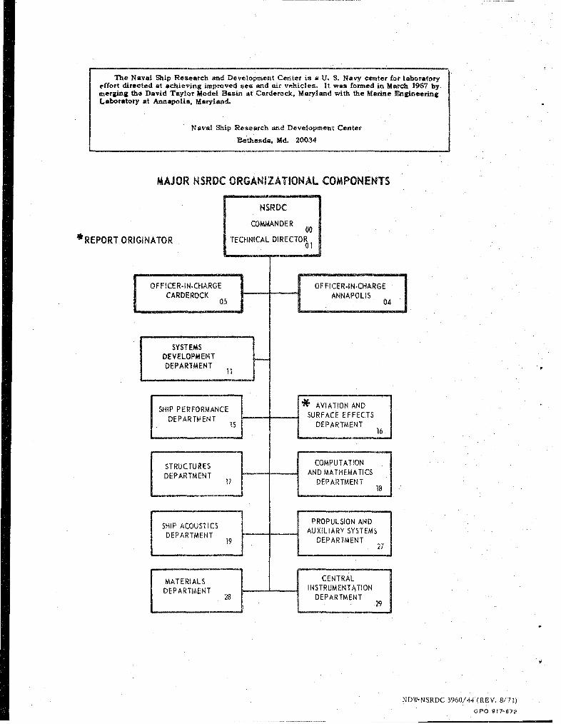
The Naval Ship Research and Development Center is a U. S. Navy center for laboratoryeffort directed at achieving improved sea and air vehicles. It was formed in March 1967 bymerging the David Taylor Model Basin at Carderock, Maryland with the Marine EngineeringLaboratory at Annapolis. Maryland.

Naval Ship Research and Development Center

Bethesda, Md. 20034

MAJOR NSRDC ORGANIZATIONAL COMPONENTS

j NSRDCCOMMANDER

00*REPORT ORIGINATOR 'TECHNICAL DIRECTOR

- ----

OFFICER-IN-CHARGE OFFICER-IN-CHARGECARDEROCK ANNAPOLIS

05 04

SYSTEMSDEVELOPMENTDEPARTMENT

S PF A AVIATION ANDSHIP PERFORMANCE SURFACE EFFECTS

15 DEPARTMENT16

STRUCTURES ICOMPUTATION

DEPARTMENT AND MATHEMATICS17 DEPARTMENT

PROPULSION ANDDEPAROUTIT AUXILIARY SYSTEMSDEPARTMENT 19 DEPARTMENT

____________________27 j

MATERIALS CENTRALDEPARTMENT INSTRUMENTATION

N 28 DEPARTMENT29

NDW-NSRDC 3960/44 (REV. 8/71)GPO 917-872

DEPARTMENT OF THE NAVY

NAVAL SHIP RESEARCH AND DEVELOPMENT CENTERBethesda, Maryland 20034

APPLICATION OF THE METHOD OF INTEGRAL RELATIONS (MIR)

TO TRANSONIC AIRFOIL PROBLEMS. PART II - INVISCID

SUPERCRITICAL FLOW ABOUT LIFTING AIRFOILS

WITH EMBEDDED SHOCK WAVE

by

Tsze C. Tai

Approved for public release;distribution unlimited.

Report 3424

July 1972 Part IIAero Report 1176

TABLE OF CONTENTS

Page

ABSTRACT ........................ .............................. I

ADMINISTRATIVE INFORMATION ................ ............... 1.

INTRODUCTION .......................... ........................... 2

BASIC FLOW EQUATIONS ........................ 4

NUMERICAL ALGORITHM . . . ................... .................... 8

METHOD OF INTEGRAL RELATIONS (MIR) ........... ............. 8

COORDINATE SYSTEMS ................... ..................... 10

STRIP BOUNDARIES AND DIVISION OF FLOW FIELD ...... ......... 10

AIRFOIL REPRESENTATION BY SPLINES ...... .............. .. 12

NUMERICAL INTEGRATION ............ .................... .. 12

Integration in Upstream Region ...... ............. .. 13

Supercritical or Subcritical Test ..... ........... .. 14

Integration along Airfoil Surface ..... ........... .. 15

Initial Values ........... .................. 16

Sonic Point ............ .................... .. 16

Shock Wave ............. .................... 17

Kutta Condition .......... .................. .. 18

Subcritical Flow ......... ................. .. 18

Integration in Downstream Region ...... ............ .. 19

Computation Time ............ .................... .. 20

TWO-POINT BOUNDARY VALUE PROBLEM - ITERATIONS ... .......... .. 21

ITERATION I - UPSTREAM INTEGRATION ....... ............. .. 21

ITERATION II - TREATMENT OF SONIC POINT .... ........... .. 23

ITERATION III - DETERMINATION OF SHOCK LOCATION ......... .. 25

ITERATION IV - INTEGRATION FOR SUBCRITICAL FLOW ......... .. 28

ITERATION V - ENFORCEMENT OF KUTTA CONDITION .. ........ .. 29

RESULTS AND DISCUSSION .............. ...................... .. 30

CONVENTIONAL AIRFOILS ............ .................... .. 30

ADVANCED AIRFOIL ............... ...................... 33

SHOCKLESS AIRFOILS ............... ..................... .. 34

CONCLUSION .................... ........................... ... 36

ACKNOWLEDGMENT .................. .......................... .. 37

ii

Page

APPENDIX A - INVISCID FLOW EQUATIONS IN A BODY-ORIENTEDORTHOGONAL SYSTEM ......... .................. .. 38

APPENDIX B - AIRFOIL REPRESENTATION BY SPLINE FUNCTION ...... .. 40

REFERENCES ................... ............................ .. 64

LIST OF FIGURES

Figure I - Coordinate Systems and Strip Boundaries ....... .. 43

Figure 2 - Geometry of a Typical Stagnation Streamline ..... .. 44

Figure 3 - A Control Surface in Inner Stagnation Region ..... .. 45

Figure 4 - Supercritical/Subcritical Test for an NACA 0015Airfoil at M = 0.729 and a = 40. . . . . . . .. . .. 46

Figure 5 - Iteration Procedures for Solving Subject Two-PointBoundary Value Problems ...... ............... .. 47

Figure 6 - Treatment of Sonic Point ...... ............... .. 48

Figure 7 - Velocity Gradients Near Sonic Point ................ 49

Figure 8 - Determination of Shock Location ... ........... .. 51

Figure 9 - Downstream Pressure Distribution for a NACA 0015Airfoil at M,,-- 0.729 and a = 40 in Upper Region . . . 52

Figure 10 - Downstream Pressure Distribution for a NACA 0015

Airfoil at Mc = 0.729 and a = 40 in Lower Region . . . 55

Figure 11 - Pressure Distribution on an NACA 64A410 AirfoilatM•= 0.72 and a =4.. . .. ............... ... 58

Figure 12 - Pressure Distribution on an NACA 0015 Airfoilat M =0.729 and a = 40 . . .. .. .. .. .. .. .. .. .. .. .. .. .. 59

Figure 13 - Pressure Distribution on an Advanced Airfoilat M = 0.70 and • = 1.50 ........................... 60

Figure 14 - Pressure Distribution on a Garabedian-KornAirfoil at M = 0.75 ....... ................. .. 61

Figure 15 - Pressure Distribution on a Neiuwland Airfoilat M = 0.7557 and a = 1.320 ....................... 62

Figure 16 - Slopes of an NACA 64A410 Airfoil at 40 = 4 ..... 63

iii

4

NOTATION

A,BQ Functions in Equation (9)

aj,bjcj,d i Constants used in Equation (B-8)

ak Constants used in Equation (10)

C C 1+ +2/[(Y-l)]C Correction coefficient

r

c Chord length of an airfoil

c Specific heat at constant volumeV

D/Dý Derivative along a streamline

E Function defined by Equations (A-10)

I An integral

K K I/(yM')

k Constant evaluated by Equation (18b)

L Lagrange multiplier function as given by Equation (12b)

M Mach number

m Coefficients used in spline function

N Number of strips; also number of points

P Static pressure normalized by its free-stream value

R Local radius of curvature normalized by the chord length

S Specific entropy

s,n Orthogonal curvilinear coordinates measured along and normalto the airfoil surface normalized by the chord length

u,v Velocity components in cartesian coordinates, normalized bythe free-stream velocity

V ,V Velocity components along and normal to the airfoil surface,s nnormalized by the free-stream velocity

V=,VV Velocity components in (t,T) coordinates, normalized by thefree-stream velocity

x,y Cartesian coordinates normalized by the chord length

x,y Rotated cartesian coordinates normalized by the chord length

1 Angle of attack

Oblique shock angle

iv

y Specific heat ratio

6 Normal distance between the airfoil surface and system

boundary normalized by the chord length

Surface inclination angle with respect to the direction of

free-stream velocity

orthogonal curvilinear coordinates measured along and

normal to the stagnation streamline normalized by the chord

length

p Static density normalized by its free-stream value

a Exponent used in Equation (22)

0 Angle between x- and x-axis

X Angle between streamline tangent and n-axis

* Angle between stagnation streamline and x-axis

Subscripts

b Conditions at airfoil surface

s Slip streamline

stag Stagnation

t Trailing edge

6 Conditions at system boundary

1 Conditions before and after shock wave

O Free-stream conditions

v

ABSTRACT

Numerical procedures developed in Part I of the presentreport for applying the method of integral relations to transonicairfoil problems are extended here to lifting cases. A modificationof the strip arrangement described in Part I now enables any desirednumber of strips and size of integration domain to be used. Thefull inviscid flow equations (may be rotational) are employed andapproximated by second-order polynomials in transverse directionin a physical plane. Numerical procedures including iterativeprocesses for solving subject two-point boundary value problemsare formulated for the case of high subsonic free-stream Machnumbers. Cartesian coordinates are employed except near theleading edge region where the use of a body coordinate systemis convenient to account properly for large slope variation there.The geometry of the airfoil is represented by cubic spline functionswhen a closed airfoil relation is not available. The effect ofchange of entropy across the embedded shock wave is examined byallowing a decrease in total pressure after the shock wave alongthe surface streamline. With the shock angle as a free parameter,oblique shock relations as well as normal shock relations can beincorporated in the solution.

Results are presented for supercritical flows past variousairfoils, including two conventional, one advanced, and two shock-less airfoils. Comparisons of the results with existing theoreticaland/or experimental data indicate reasonably good agreements. It isfound that the shock location moves forward in the case of a finiteincrease in entropy across the shock wave; the change of entropyhas, therefore, a cumulative effect on the flow.

ADMINISTRATIVE INFORMATION

The work presented in this report was supported by the Naval Air

Systems Command (AIR-320) under NAVAIR TASK R230.201.

INTRODUCTION

The problem of inviscid transonic flow past a prescribed airfoil has

been studied by using numerical procedures based on the method of integral

relations. The results of the investigation are reported at different

stages of completion. Part I of this report presented the numerical pro-

cedures and exploratory results for flows over symmetric airfoils at zeroi

angle of attack. Since then, the method has been extended to lifting

airfoils. The flows are also inviscid supercritical, with embedded shock

waves. The work of this stage is now described as Part II.

Since Part I was published in September 1970, research effort on

transonic flows has been phenomenal as reflected by the number of survey and/

or review papers that have appeared during this interim period. A survey

paper by Newman and Allison2 lists a large number of theoretical papers

relating to steady inviscid external transonic flows and provides up-to-date

information for assessing the state of the art. Three review papers on

theoretical methods in transonic flows have recently been published; sequen-3 4 5

tially these are by Murman, Norstrud, and Yoshihara. The Norstrud paper

summarizes available analytical and numerical methods for the solution of

an appropriate transonic flow problem and covers a broad range of transonic

flows. The papers by Murman and Yoshihara, on the other hand, are more or

1. Tai, T.C., "Application of the Method of Integral Relations toTransonic Airfoil Problems: Part I - Inviscid Supercritical Flow overSymmetric Airfoil at Zero Angle of Attack," NSRDC Report 3424 (Sep 1970);also presented as Paper 71-98, AIAA 9th Aerospace Sciences Meeting, NewYork, N.Y. (Jan 1971).

2. Newman, P.A. and D.O. Allison, "An Annotated Bibliography onTransonic Flow Theory," NASA TM X-2363 (Sep 1971).

3. Murman, E.M., "Computational Methods for Inviscid Transonic Flowswith Imbedded Shock Waves," Boeing Scientific Research LaboratoriesDocument DI-82-1053 (1971); also presented in AGARD-VKI Lecture Series onNumerical Methods in Fluid Dynamics, Rhode-Saint-Genese, Belgium (Mar 1971).

4. Norstrud, H., "A Review of Transonic Flow Theory," Lockheed-Georgia Company, Report ER-11138(L) (Aug 1971); also presented as Paperat University of Illinois Seminar (Mar 1971).

5. Yoshihara, H., "Some Recent Developments in Planar InviscidTransonic Airfoil Theory," AGARDograph 156, North Atlantic TreatyOrganization (Feb 1972).

2

less confined to the area of computational methods. The former treats

existing methods for flows with embedded shock waves. The latter is con-

cerned with the hodograph method for shockless flows and finite difference

schemes for more general flows. Both papers emphasize methods based on

the use of finite difference procedures.

The method of finite differences is a highly developed numerical pro-

cedure. It is generally not difficult to select a difference scheme to

approximate the differential equations in a stable manner, and the method

is well suited for application to transonic flow problems. An example6

is the time-dependent approach of Magnus and Yoshihara. The computations

are lengthy, however. It is more economical to use small disturbance

equations with relaxation procedures, as employed by Murman and Cole. 7

The disadvantage of using these equations, however, is that they preclude

the important class of airfoils with blunt noses and these are currently* 8

of interest. Steger and Lomax employed a more realistic system consist-

ing of inviscid, fully nonlinear, potential flow equations. Their approach

proved to be fruitful; its only drawback was that the system of equations

used does not allow an entropy (or total pressure) change across the shock

wave. Although the change of entropy is normally small in transonic flows,

it may influence the location of the shock wave (because of the change of

the downstream conditions), and thus alter a considerable portion of the

entire flow. This point is sometimes overlooked.

Because of the various difficulties involved in using finite difference

*In a private communication, however, Dr. Murman indicated that although

the small disturbance equations were not valid for blunt-nosed airfoils,his overall result was surprisingly not greatly affected by nose bluntness.

6. Magnus, R. and H. Yoshihara, "Inviscid Transonic Flow over Airfoils,"General Dynamics/Convair Division Report (1969); also presented as Paper70-47, AIAA 8th Aerospace Sciences Meeting, New York, N.Y. (1970).

7. Murman, E.M. and J.D. Cole, "Calculation of Plane Steady TransonicFlows," AIAA J., Vol. 9, No. 1, (Jan 1971), pp. 121-141 (AIAA Paper No.70-188, 1970).

8. Steger, J.L. and H. Lomax, "Numerical Calculation of TransonicFlow About Two-Dimensional Airfoils by Relaxation Procedures," presentedas AIAA Paper 71-569 at AIAA 4th Fluid and Plasma Dynamics Conference,Palo Alto, California (Jun 1971).

3

schemes, it is natural to take an alternative approach, such as the method

of integral relations (MIR) employed in the present report. Other recent

applications of the method to transonic flows past airfoils include those9 10 11

by Holt and Masson, Melnik and Ives, and Sato. However, these studies

are confined to subcritical flows or supercritical flows over symmetric

shapes using only two strips.

In the present report, the basic numerical procedures described in

Part I are extended to lifting arbitrary shapes and subsequently refined.

The enforcement of the Kutta condition is accomplished by adding one more

iteration to the previous procedures. The use of full inviscid non-

isentropic equations allows an entropy change across the shock wave. The

airfoils considered include two conventional airfoils, two shockless air-

foils, and one advanced (supercritical) airfoil, all at supercritical flow

conditions corresponding to M. < 1 transonic regime.

BASIC FLOW EQUATIONS

The basic flow equations for the lifting cases are the same as those

used in Part I except that nonisentropic jump is introduced across the

shock wave. For the sake of convenience, they are repeated here

Continuity:au + 6(PV) = 0 (1)

9. Holt, M. and B.S. Masson, "The Calculation of High Subsonic FlowPast Bodies by the Method of Integral Relations," Second InternationalConference on Numerical Methods in Fluid Dynamics, University of California,Berkeley (Sep 1970).

10. Melnik, R.E. and D.C. Ives, "Subcritical Flows of Two-DimensionalAirfoils by a Multistrip Method of Integral Relations," Second InternationalConference on Numerical Methods in Fluid Dynamics, University of California,Berkeley (Sep 1970).

11. Sato, J., "Application of Dorodnitsyn's Technique to CompressibleTwo-Dimensional Airfoil Theories at Transonic Speeds," National AerospaceLaboratory Technical Report TR-220T (Tokyo, Japan) (Oct 1970).

4

x-Momentum:

S(KP + pu 2 ) + - (puv) = 0 (2)

y-Momentum:

aa(uv) +y(KP+ pv) = 0 (3)

These equations are written in a Cartesian coordinate system, governing

a steady, adiabatic inviscid fluid flow. The lengths are normalized with

respect to the chord length, and pressure, density, and velocity components

are normalized with respect to their free-stream values. The symbol K

represents

K1

where for air, y = y. = 7/5.

The boundary conditions are as follows:

At the airfoil surface, the normal velocity component is equal to zero, i.e.,

V = u sin e + v cos e = 0 (4a)n

where e is the surface inclination angle with respect to the direction of

free-stream velocity.

At infinity, the flow is undisturbed, i.e.,

P pu 1

v =0 (4b)

One more equation is needed in order to determine four dependent

variables u, v, p, and P. It is the isentropic relation between the

density and static pressure

P = py (5a)

This is good for regions before the shock wave and the far field. For

regions after the shock wave, where the fluid has a finite increase in

entropy (or a decrease in the total pressure), it becomes

5

P = EXP - p (5b)cV

The change of entropy (S 2 -S 1 ) is normally small for transonic flows.

However, as will be discussed later because of the corresponding change

of the downstream conditions, it may influence the location of the shock

wave and thus alter considerable portions of the entire flow. Nonethe-

less, the flow behind the shock wave is still isentropic along a streamline

(which serves as strip boundary). The new isentropic relation, however,

is based on a new entropy level which is slightly higher than its free-

stream value. The new entropy level differs from one streamline to the

other because the shock strength encountered on each streamline differs.

The value of new entropy level is obtained through the following

relation

(S2 - S1\ P2EXP Cv = P (6)

where P2 and P2 are the static pressure and density immediately after the

shock. For an inviscid flow, the shock is normal at the surface in order

to keep the flow attached. The Rankine-Hugoniot relations for normal

shock waves are appropriate here for determining P2 and P2. They are:

(y-l) M12

P2 = Pi (7a)(y-l) M 1

2 + 2

P2 = PI [I + 2A-' (M12 _ I)] (7b)

Subscripts 1 and 2 respectively denote values in front of and behind the

shock wave.

It is well known that the shock is curved away from the surface.

Therefore oblique shock relations must be used for the intermediate strip

boundary.

P2 = P1 (+l)(MI sin p)2 (8a)(y-I)(M1 sin 0)2 + 2

6

P2 = P1 +2y (MI 2 sin2 • - i)! (8b)

where • is the shock angle with respect to the local streamline direction.

When • = 90 degrees, Equations (8) become the normal shock relations.

In fact, the Rankine-Hugoniot relations are contained in the system

of Equations (1) - (3) if the latter are applied along a streamline. Use

of the normal shock relations at the foot of the shock wave is known to

be questionable. Emmons12 found that the Rankine-Hugoniot relations

lead to infinite curvature where the shock touches the curved wall of

the airfoil. Sichel13 proposed a model which accounts for the non-Rankine-

Hugoniot nature of weak shocks near the wall. The Sichel model includes

a viscosity term to give a system of viscous transonic equations for the

non-Rankine-Hugoniot region. It is difficult to solve these equations

mathematically, but it has been demonstrated that an oblique shock wave

represents an exact similarity solution.

On the basis of the above arguments, therefore, the normal shock value

for the shock jump condition at the foot of the shock could be in great

error for certain cases. In such cases, an oblique shock jump should

correlate the flow better than the normal shock jump. The angle of the

oblique shock, of course, cannot be resolved without considering the

viscous-inviscid interaction. An empirical curve of the pressure ratio

before and after the shock foot was determined by Sinnot. 1 5

There are limiting cases in which the strength of the shock is so

weak that it can be considered as a series of compression waves. The flow

12. Emmons, H.W., "Flow of a Compressible Fluid past a SymmetricalAirfoil in a Wind Tunnel and Free Air," NACA TN 1746 (Nov 1948).

13. Sichel, M., "Structure of Weak Non-Hugoniot Shocks," Physics of

Fluids, Vol. 6, No. 5, pp. 653-662 (May 1963).

14. Ferrari, C. and F.G. Tricomi, "Transonic Aerodynamics,"Translated by R.H. Cramer, Academic Press (1968).

15. Sinnot, C.S., "On the Prediction of Mixed Subsonic/Supersonic

Pressure Distributions," J. Aerospace Sciences, Vol. 27, pp. 767-778(1960).

7

is then the so-called "shockless" solutions or the "weak solution"

to the subject boundary-value problem.1 9

In order to be consistent with the inviscid model, the normal shock

relations are applied in the present study at the foot of the shock wave.

In some cases, options of oblique shock values are also provided with

the shock angle as a free parameter. Furthermore, it is assumed that the

embedded shock wave is steady under the imposed boundary conditions.

NUMERICAL ALGORITHM

METHOD OF INTEGRAL RELATIONS (MIR)

The feasibility of applying the method of integral relations to

supercritical flows over symmetric airfoils at zero angle of attack has

been studied and demonstrated in Part I of the present report. Necessary

numerical procedures were described and a new strip arrangement was intro-

duced which allows the free-stream condition to be set at "infinity."

The approach is now extended to lifting cases.

Briefly, in applying the method of integral relations, the system of

flow equations must be written in divergence form:

A(x,y,u,...) + -a B(x,y,u,...) = Q(x,y,u,...) (9)ax 6y

The divergence form of Equations (1) - (3) may then be integrated outward

from the airfoil surface (but not necessarily normal to the surface) to

each strip boundary successively at some constant value of x. This

16. Nieuwland, G.Y., "Transonic Potential Flow around a Family ofQuasi-Elliptical Aerofoil Sections," National Aerospace Laboratory(Amsterdam) Technical Report T-172 (Jul 1967).

17. Korn, D.G., "Computation of Shock-Free Transonic Flows forAirfoil Design," New York University Courant Institute of MathematicalSciences, Report NYO-1480-125 (Oct 1969).

18. Boerstoel, J.W. and R. Uijlenhoet, "Lifting Airfoils withSupercritical Shockless Flow," ICAS Paper 70-15, 7th Congress of theInternational Council of the Aeronautical Sciences, Rome, Italy (Sep 1970).

19. Morawetz, C.S., "The Dirichlet Problem for the Tricomi Equation,"Convn. Pure Appl. Math, Vol. 23, pp. 587-601 (Jul 1970).

8

procedure reduces the partial differential equations (with independent

variables of x and y) to ordinary ones (with independent variable x)

In order to perform the integration, the variation of integrand along y

must be known. A general approach is to approximate the integrands by

interpolation polynomials, for example, A by

N

A = N ak(x)(Y - yo)k (10)

k=0

where N is the number of strips and ak are constants evaluated at strip

boundaries. In principle, the actual flow variation may be represented

more closely by an increasing number of strips.

Ordinary differential equations derived by using a second-order

polynomial were presented in Part I. These equations are also used to

calculate lifting cases in the present report. In the lifting case,

however, they are applied separately for both upper and lower flow fields.

The division of the flow fields will be discussed later.

In order to examine higher order effect in the MIR, a set of ordinary

differential equations is derived by using a regular third-order poly-

nomial. The system was coded first for the computation of upstream flow.

The use of third-order equations was found to be less stable than second-

order equations. This instability is attributed to a negative value of

dv/dx generated in the first few steps of integration in the upstream

region. This negative dv/dx is contradictory to physical phenomenon and

entirely caused by the mathematical inflection point of the third-order

polynomial. Not every third-order polynomial has an inflection point.

However, it easily becomes inflected if the (third-order) polynomial is

representing a transverse flow variation from the undisturbed free stream

(straight line) to a disturbed state. Possibly it would have worked

better than the second-order equations in other flow regions, but in any

event, the computation has to start from the upstream region. Complexity

is another unpleasant feature of third-order equations. For these reasons,

they are no longer employed.

9

COORDINATE SYSTEMS

Similar to the nonlifting case, Cartesian coordinates are employed

as the basic coordinates. In the leading edge region where drastic changes

of body slopes are involved, a body-oriented orthogonal curvilinear

coordinate system is incorporated. The latter is embedded in the former

(Figure 1). The solution of the outer region interacts with that for the

inner region. Since the width of the inner region is normally fairly

thin, one-strip approximation is used in this region. Part I of this

report presented ordinary differential equations reduced by using one-

strip approximation in the orthogonal curvilinear coordinates. The system

is revised in Part II by the addition of a momentum equation to account for

the effect of body properties on the outer flow. The present forms are

given in Appendix A.

There are two reasons for using the above coordinate systems in the

physical plane. First, the method of integral relations is a universal

numerical method. If no particular advantage can be secured by using any

sophisticated transformation, convenience surely should prevail. This is

particularly so when modern high-speed computers are available. Second,

in calculations of supercritical flows where there are mixed (elliptic-

hyperbolic) flow characters, it is difficult to select a function as a

basis of transformation to a computational plane. For example, functions

based on incompressible solution (such as used by Chushkin 20-22) become

highly inadequate in the present case.

STRIP BOUNDARIES AND DIVISION OF FLOW FIELD

Even though no transformation of coordinates is involved, the free-

stream boundary can still be set at "infinity" in the present study. This

is implemented by a new arrangement of strip boundaries. As described in

20. Belotserkovskii, O.M. and P.I. Chushkin, "The Numerical Solutionof Problems in Gas Dynamics," "Basic Developments in Fluid Dynamics,"Vol. 1, edited by M. Holt, Academic Press (1965).

21. Chushkin, P.I., "Subsonic Flow of a Gas past Ellipses andEllipsoids," Translation of Vychislitel'naya Maternatika (USSR), No. 2,pp. 20-44 (1957).

22. Chushkin, P.I., "Computation of Supersonic Flow of Gas pastArbitrary Profiles and Bodies of Revolution (The Symmetric Case),"Translation of Vychislitel'naya Maternatika (USSR), No. 3, pp. 99-110 (1958).

10

Part I, the idea is to treat the whole integration domain as a series of

different effective regions; a small number of strips may be used within

each region. The whole integration domain with free-stream as its outer

boundaries can be set as large as desired. It then corresponds to an

application of the free-stream boundary at "infinity." A significant

advantage of this new arrangement, however, is that it allows the use of

a large number of strips without the need for higher order polynomials

which usually cause numerical difficulties in actual computation.

Similar to nonlifting cases, some typical streamlines are used as

strip boundaries in the present approach. In the lifting case, however,

the upper and lower flow fields are divided by the streamline passing

along the airfoil surface. In the upstream region, this streamline is

called the stagnation streamline. It splits into the upper and lower

surfaces of the airfoil on striking at the stagnation point and meets

again at the trailing edge (for the present inviscid flow). After leaving

the trailing edge, it flattens out and asymptotically approaches an

undisturbed state far downstream.

The equations for determining the stagnation streamline geometry are23derived by using a procedure similar to that presented earlier. They

are given below.

Dx -cos • (lla)

Dy = sin 4 (lib)Dt

1 (isin cos * • (llc)

The geometry of a typical stagnation streamline is shown in Figure 2.

Five strips are used in the far field of the upstream region and

eight in the near field of this region for both upper and lower sides.

Six strips are employed for the leading edge region including the strip

associated with the orthogonal curvilinear coordinates. The number may

23. Tai, T.C., "Streamline Geometry and Equivalent Radius over aFlat Delta Wing with Cylindrical Leading Edge at an Angle of Attack,"NSRDC Report .3675 (Oct 1971).

11

be reduced to five in case the sonic line might touch the nearest strip

boundary. Four or five strips are mostly used for the airfoil region

depending on the flow condition or the local airfoil curvature. In the

downstream region, the number of strips can even be decreased to three.

The outermost strip boundary (free-stream) is set about seven chord lengths

away from the airfoil. The above strip arrangement is based somewhat on

a compromise between accuracy and numerical instability. An important

factor for the setup of course is that it allows the recovery of the

free-stream values in the far downstream for the sake of existence and

uniqueness of the solution as discussed later. The schematic view of

the strip arrangement is shown in Figure 1.

AIRFOIL REPRESENTATION BY SPLINES

In analyzing transonic lifting airfoil problems by using the method

of integral relations, difficulty has been encountered in obtaining

continuous first- and second-order derivatives of the airfoil surface.

This is because only tabulated coordinates are available for airfoils

other than the NACA four-digit family. In the process of numerical sol-

ution, those tabulated coordinates must be transformed to a curve through

the curve-fitting technique. Of the various techniques available for

numerical interpolation, the cubic spline function was found to be best

suited for curve-fitting purposes because the function and its first- and24

second-order derivatives are continuous in the whole range. Accordingly,

the cubic spline function is employed for representing arbitrary airfoils.

Equations of the cubic spline function used for airfoil representation

are presented in Appendix B.

NUMERICAL INTEGRATION

With the partial differential equations reduced to a set of ordinary

differential equations by the method of integral relations, the numerical

integration may be carried out along the longitudinal axis x by using a

standard scheme such as the fourth-order Runge-Kutta method. The details

of the integration for each region are described below.

24. Ahlberg, J.H. et al., "The Theory of Splines and Their Applications,"Academic Press (1967).

12

Integration in Upstream Region

The numerical integration first starts from the upstream region

sufficiently far away ahead of the airfoil, say, approximately four chord

lengths. Integrations for both upper and lower flow fields are carried

out simultaneously. Physically, the uniform flow here is disturbed by

the presence of the airfoil. The velocity will decrease along some

streamlines and increase along others. In particular, the velocity

along the stagnation streamline will monotonically decrease to zero.

Thus, the behavior of the stagnation streamline provides a constraint

in determining the flow field in the upstream region. Once the velocity

along the stagnation streamline decreases, the whole upstream flow field

ought to vary accordingly. This concept is implemented in our computation

in order to create the flow variation far upstream. Practically, the

velocity along the stagnation streamline is forced to decrease by applying,

an artificial disturbance in the beginning of the integration. After a

few steps, a transverse velocity gradient along the stagnation streamline

is created by the overall flow field. It causes the velocity along the

stagnation streamline to decrease. As soon as the system begins to work

stably, the artificial disturbance is taken away.

The integration for the upstream region ends at a station in front

of the airfoil. The flow along the stagnation streamline is further

extrapolated to the stagnation point with a third-order Lagrange polynomial:

3

u(x) = Li(x)ui (12a)

i=O

where Li(x) is the Lagrange multiplier function

L (x-xo) (x-x).. . (x-xi- 1 ) (x-xi+l)... (x-xN) (12b)i (xi-xo)(xi-xi)... (xi-xl)(xi-xi+i)...(xi-xN)

At this stage a test is made to determine whether the flow along the

airfoil will become supercritical or subcritical.

*This artificial disturbance is not an arbitrary one, however. Its form

and strength are determined by satisfying the terminal condition at thestagnation point. The procedure involves an iteration process which willbe discussed later in greater detail.

13

Supercritical or Subcritical Test

The present study considers supercritical flows over a lifting airfoil.

The flow over the upper surface of the airfoil will be supercritical while

that over the lower surface usually remains subcritical. The great majority

of transonic airfoil flows fall into this category. Quite often, however,

flows over both sides of the airfoil can be either supercritical or sub-

critical, depending on the free-stream Mach number and angle of attack.

Thus, we have to determine which side of the airfoil will have supercritical

or subcritical flows before we proceed with the numerical integration

along the airfoil surface.

The test is based on the control surface in the leading edge flow

field (Figure 3). Some approximate values of Vsb at several points away

from the stagnation point are determined by the law of conservation of

mass in the control surface. For the control surface abcd, the mass flux

entering line cd should equal to the mass flux leaving line bc, i.e.,

c c

pudy = pVsdn (13)J Td b

The integration of the left-hand side is performed easily since the

distribution of pu along line dc is known. The integral on the right-hand

side, however, has to be approximated by a linear distribution in pVs:

c

6PVsdn - T (PbVsb + PcVsc) (14)

where pc and Vsc are known quantities at point c. Upon equating Equations

(13) and (14) we obtain

.2Vsb P Pudy - PcVsc /Pb (15a)

Sb 6 b

where Pb is determined by the law of conservation of energy with the aid

of isentropic relations:

14

1

C - Vsb y-Ilb= - C - 1i (15b)

and

C = 1 + (y (15c)

Note that Equation (15b) is good only for the flow before the shock wave.

The procedure is repeated to determine Vs values at points b,, b2,

and b3 (Figure 3). The resulting values are then extrapolated with the

third-order Lagrange formula to certain distances downstream to determine

whether it will become supercritical or subcritical. The same procedure

is employed for the lower side of the flow.

A typical example for this test is demonstrated in Figure 4 which

shows the result for an NACA 0015 airfoil at M.= 0.729 at ct= 4 degrees.

Broken lines indicate extrapolated values. If the flow is supercritical,

the extrapolated Mb should exceed unity. Otherwise, it remains subcritical

(Figure 4).

The error of linear approximation of Equation (14) becomes greater

as the distance between the two ends 6 increases. As indicated in Figure

3, the lower side certainly suffers greater error than the upper side.

In any case, it is just a preliminary test to choose options relative to

supercritical or subcritical flow for computations along the airfoil

surface. The results of the present test have no significance for the

computations given below.

Integration along Airfoil Surface

The above test indicates which side of the airfoil will be supercritical

or subcritical. The present study is primarily concerned with supercritical

flows; subcritical flow is considered as a special case which may happen

over the lower surface of the airfoil. The basic equations to be used,

however, are common for both flows. For the leading edge region, both

flows use a mixed system which consists of equations associated with

Cartesian coordinates for the outer portion and orthogonal curvilinear

15

coordinates for the inner portion. The mixed system is used in order to

account for large surface derivatives in the leading edge region.

Initial Values. The numerical integration along the airfoil surface

starts from a constant x-axis where the upstream region integration ended.

In a mixed system formulation, this constant x-axis location is connected

by a straight line normal to the airfoil surface. As an illustration, it

is the line bc in Figure 3. The constant x-axis is xo-axis. The point

at the foot of this normal line corresponds to the "initial point" at the

airfoil surface. That is point b in Figure 3. The distance between the

x0 -axis and the airfoil stagnation point 6 is not known in advance. It

can be roughly determined by extrapolating the stagnation streamline to

the stagnation point as mentioned previously.

The precise determination of 60 involves another iteration process

which will be discussed in detail in the next section. Once this distance

is determined, it is a simple matter to find the initial values at the -

initial point. This is accomplished by integrating the one-strip equations

in the inner stagnation region (Figures 1 and 3) to the initial point.

No difficulty is encountered in performing the integration since all values

are known along the system boundary (line cd in Figure 3). The effect of

inaccuracies introduced by the one-strip approximation here will be absorbed

in the process for determining the distance 6o as discussed later.

Sonic Point. The integration of the mixed system now proceeds. The

velocity along the surface accelerates rapidly. In order to avoid diver-

gence of numerical results at the singular point, the integration of the

inner system is replaced by a curve fit in the neighborhood of the sonic

point. This is accomplished by using a third-order Lagrange polynomial.

The singular behavior near the sonic point will be discussed in the next

section. The integration continues after the sonic point (at the airfoil

surface). Now there is a small supersonic region near the airfoil surface.

As soon as the surface slopes become moderate, the mixed system is replaced

by the regular Cartesian system. As the supersonic region grows, the sonic

line might touch the first-strip boundary. In this case, that strip

boundary is dropped in order to avoid numerical difficulty there.

16

The integration is then operated at one less number of strips.

Shock Wave. The supersonic region is generally terminated by a shock

wave. If the strength of the shock wave is strong enough, the flow should

be back to subsonic again. If it is weak, the flow may still remain in the

supersonic state or in the subsonic state but further expand to supersonic

again. In this latter case, the occurrence of multiple shock waves is pos-

sible. The method of integral relations, as formulated, allows only one

shock wave to appear. This is because the uniqueness condition has to be

satisfied, as discussed in the next section. For a given shock wave

location, the shock wave relations are applied along the surface stream-

line. The shock wave is not inserted on other strip boundaries since

the supersonic region for (supercritical) flows of practical interest is

not tall enough to reach the existing first-strip boundary; fewer strips

are needed from the sonic region on, and therefore the first-strip boundary

can be set as high as 0.7 chord lengths away. This height of the first-

strip boundary almost covers all supercritical flows of practical interest.

For instance, shockless flows generally have a larger supersonic pocket

(due to the "peaky pressure distribution") than those with an embedded

shock. The following is a survey on the tallest supersonic region from

existing shockless solutions:

Tallest Supersonic Region Source

(chord length, c)

0.250 Nieuwland16

0.545 Korn17

0.254 Boerstoel and Uijlenhoet 1 8

There is no solution that has a supersonic region even taller than 0.6c.

The determination of the shock location involves another iteration which

is explained in the next section.

An important advantage of the method of integral relations is its

flexibility in applying the shock wave relations. Here one can use the

normal shock relations, Equations (7), or the oblique shock relations,

Equations (8). After the shock wave, one can use Equation (5a) for a

potential flow solution or Equation (5b) for a nonisentropic solution.

17

The overall effects of the entropy change across the shock wave and the

shock angle on the flow can therefore be easily examined, although this

is difficult to do in other existing methods. The change of entropy is

third-order in (MI - 1), but its effect on the flow is cumulative because

of its influence on the shock location.

Right after the shock wave, the numerical integration continues.

There is a short expansion of the flow because of change of airfoil

curvature. This is then followed by a deceleration region down to the

trailing edge. If the airfoil curvature changes appreciably in this

region, one more strip may be added to get the desired sensitivity.

Kutta Condition. When the numerical integrations along the upper and

lower surface reach at the trailing edge, their resulting static pressure

should be equal. This is the Kutta condition for a sharp trailing edge.

Unlike the relaxation technique, no apparent circulation term is treated

in the present formulation. Circulation exists, of course, in the sense

of different velocity distributions along the upper and lower surfaces

of the airfoil. The requirement of equal pressures at the trailing edge

from both upper and lower surface integrations involves another iteration

process which will be given in the next section.

Subcritical Flow. As mentioned above, the flow over the lower surface of

the airfoil could be subcritical for a moderate supercritical flow over

the upper surface. Thus, we have to provide options for subcritical flow

over the lower surface of the airfoil. In this case, the problem of the

singular point and the determination of the shock wave are omitted. With

the exception of these simplifications, the procedure for numerical

integration follows the same pattern as for the upper surface. That is,

a mixed system is used for the leading edge region and a regular Cartesian

system for the rest of the airfoil surface. The number of strips may also

vary according to the surface curvature. The height of the outermost

strip boundary is about the same as that for the upper surface. Also,

the distance 6o between the x0 -axis and the stagnation point is the same

as determined for the upper surface.

The only problem with the lower surface is the inadequacy of

18

the one-strip approximation for the inner stagnation region. Note from

Figure 3 that the distance variable 6 for the lower surface is approx-

imately 50 percent longer than that for the upper surface. The longer

this distance, the less accurate the one-strip approximation. The

inaccuracy is actually attributed to the fact that the ratio of this

distance to the local radius of curvature is too large. In this case, a

twO-strip approximation should give much better results. There is no

problem in deriving a set of second-order equations for this inner region,

but there is difficulty in evaluating the initial conditions for the

middle strip boundary. For this reason, rather than attempt to use a

two-strip approximation here, a correction is made in the radius of cur-

vature for the one-strip system, i.e., let

R = CrRb + 6 (16)

where C is the correction coefficient which has values 2.0 : C Ž 1.0.r rIt was found that values of C = 1.5 to 2.0 were appropriate for mostr

cases. No such correction is used for the upper surface, i.e., C = 1.0.r

Possibly it too needs correction for the upper surface integration. How-

ever, as mentioned before, the inaccuracies there could have been absorbed

and compensated in the process of determining y. or 60.

Integration in Downstream Region

The procedure for integration in the downstream region is somewhat

the reverse of that for the upstream region. Here we expect that the

integration will result in a uniform flow in the far downstream. The

integration starts at the trailing edge. Although the static pressure

is the same for the upper and lower surfaces at the trailing edge, the

velocities are not equal because of the total pressure change at the shock

wave. Therefore, a slip streamline emanates from the trailing edge.

The numerical integration is carried out simultaneously for both the upper

and lower flow fields with the slip streamline as the dividing boundary.

In order to simplify the procedure, the shape of the slip streamline is

determined in such a way that its vertical velocity component v vanishesS

asymptotically in the downstream. This kind of variation in vs is easily

represented by an exponential curve with the property of asymptotical

19

decay, i.e.,

vs = vte -k(x-xt) (17a)

and

(dý vs (17b)dx) s us

Therefore, the geometry of the slip streamline is:

r v-k(x-xt)

ys = U t dx + yt (18a)

where subscripts s and t denote values along the slip streamline and at

the trailing edge, respectively. The constant k is determined by satis-

fying the gradient of vs at the trailing edge. Therefore we find

k I dvs L (18b)L vs dx-jt

which gives positive value for k.

In principle, similar procedure as employed in the upstream region

may be used. A numerical experiment shows that the above procedure

ensures numerical stability in the far downstream region.

Computation Time

A typical converged run on a CDC 6700 computer takes about 45,000

storage capacity (minimum required storage for CDC 6700) and an average

of 0.04 sec per step size for various strip arrangement. A total of

700-1000 steps are needed for integration from upstream to downstream.

This amounts to about 30 to 40 sec for a converged run. To take account

of iterations as described in the next section, the above figure has to

be increased 30 to 90 times. That is, the total computation time will be

somewhat between 15 min to 1 hr on the CDC 6700, including necessary

iterations. The computer program was written on the basis of convenience

rather than efficiency. No attempt has been made to optimize the program.

It is expected that computational experience will certainly help to cut

down the number of iterations.

20

"TWO-POINT BOUNDARY VALUE PROBLEM- ITERATIONS

Mathematically, the problem of transonic flow past an airfoil is a

boundary value problem. The overall solution not only has to satisfy

the governing equations but is also subject to boundary conditions. When

the governing partial differential equations are reduced to ordinary set

by some means, such as the method of integral relations in the present

study, the problem becomes a two-point boundary value problem. The gen-

eral strategy for solving the subject two-point boundary value problem

is the so-called initial value technique. In this technique, initial

values for the integration are estimated and iterated from time to time

until the imposed or terminal conditions are satisfied. The solution

procedure consists of iteration processes.

Five iteration processes are involved in the present study. They

are illustrated in Figure 5 and described in detail below.

ITERATION I - UPSTREAM INTEGRATION

The upstream flow is influenced by the presence of the airfoil.

As mentioned in the previous section, the variation of the upstream flow

initially starts through an artificial disturbance. The form of the

disturbance, however, depends on the properties at the stagnation point.

With reference to the •, T coordinates which are conveniently

employed for the orientation of the stagnation streamline (see Sketch 1),

Sketch I

TI,V

ý, V

21

the continuity and I-momentum equations are written as follows:

at (PV0) + - [(1 + )pV1J] = 0 (19)

S(pV§e + KP) + [(1 + )pVV•] -pvv (20)

SR

Note that these equations are exactly the same as Equations (A-l) and

(A-2) of Appendix A if (Q,T) coordinates are replaced by (s,n) coordinates.

Along the stagnation streamline where T = 0 and V 0 , Equations (19)

and (20) can be reduced to the following form:

( 1(21)

Equation (21) governs the velocity along the stagnation streamline. The

velocity V decreases monotonically toward the stagnation point since

M < 1 and (OV /Yf§V)mO > 0. The change in V also provides a guideline

for the variation of the upstream flow since the equations governing the

whole upstream flow field involve V•.

The disturbance is created here in terms of the transverse velocity

gradient 6V /6ý. It then causes V to decrease. It is assumed that its

magnitude in the upstream varies with its stagnation value according to

a power law

6= (.~( ~(22)

(26,Th0,ý:O 6stag (xsta

For calculation purposes, a value of a = 4 was used (a numerical experiment

shows that a = 4 is appropriate). Both (6V /aThstag and xstag are not known

in advance and have to be estimated for the first time.

With the aid of Sketch 1, we find

( )5~ (2 3a )

s~ dsgstag stag

And with one-strip approximation,

22

'dVsb P6Vd6 6sd (P6Vs - 2(i + R-)P6Vn6d s ('V 6 - 2 + (23b)

ds stag 6oPstag

Terms on the right-hand side are known after the integration reaches the

x0 -axis and are extrapolated to the stagnation point. The extrapolated

value for 60 can be further improved by iteration for the singular point.

The known quantities are then susbtituted into Equations (23) and the

new values for both (6VI/'Tstag_ and xstag are generally different from

those previously estimated. The procedure is repeated until final con-

vergence is achieved. The significance of the iteration here is its

provision of the flow feedback from the airfoil to the upstream region

as characterized by elliptic equations.

As mentioned in the previous section, the disturbance is applied

only for the first several steps in the upstream integration. A rapid

convergence is therefore obtained for this kind of iteration. The

iteration has only a slight effect on the final result. Thus it is a

weak iteration.

ITERATION II - TREATMENT OF SONIC POINT

For supercritical flows, the ordinary differential equations have

at least one saddle-type singularity at the sonic point(s) (or near the

sonic point if the equations are written in Cartesian coordinates).

This is indicated in Equations (A-4) of Appendix A (and in other du/dx

equations given in Part I) where the denominator goes to zero when M = 1.

Physically, however, there should be a continuous flow through the sonic

point(s). A continuous solution exists only if the numerator and denom-

inator of that equation simultaneously become zero so that the ratio

0/0 still yields a finite quantity. In order to force the numerator to

zero when M - 1, adjustment of certain unknown parameter(s) in the course

of the solution is involved. The present iteration, therefore, adjusts

certain unknown parameters (this is a common procedure for solving a two-

point boundary value problem) so that a continuous solution exists at

the sonic point.

It is appropriate to use the physical parameter(s) as the varying

parameter(s). More than one parameter may be found to have pertinent

23

physical significance. At the same time, more than one strip boundary

may possibly have a sonic point in the present formulation. This usually

happens in the case of certain flow conditions where the sonic region

crosses more than one strip boundary. In order to simplify the procedure,

however, the present study considers only flows with moderate sonic region

which do not cross more than one strip boundary. In fact, as discussed

in the previous section, most practical flows fall into this category.

As a consequence, there is only one sonic point which occurs on the

surface boundary. In this case we have to choose a physical parameter

as the varying parameter and fix all others, if any.

The height of the outermost strip boundary was used as the varying

parameter in Part I of the present report. This outermost boundary

location was introduced in Part I to modify the original infinite integra-

tion domain to a finite one. Since the strip spacing is a function of

this height, it has direct effect on the initial condition such as the

velocity gradient at the initial point. Thus, it is a physical parameter.

Its value will be precisely determined in the present iteration in order

to obtain a continuous solution through the sonic point. The idea is

analogous to the hypersonic blunt-body problem in which the adjustment

of the shock standoff distance is required for a continuous solution

through the sonic point (see Figure 6).

In fact, the above procedure eventually absorbs all the constituents

of the inaccuracies in the initial condition for obtaining a smooth

solution through the sonic point. These inaccuracies may be attributed

to polynomial approximation, strip arrangement, numerical truncation,

approximated values for some physical parameters, and so forth. If one

of the above sources of inaccuracy is changed, the varying parameter has

to be adjusted over again. Thus, determination of the unknown parameter

is based on a combination of fixed values for all other extraneous and

*Note that the adjustment of the outermost strip boundary (free-streamboundary) does not contradict the argument for imposing the free-streamboundary as far as possible. In fact, the solution is dictated by theparticular integration scheme used. For instance, the three-two-stripintegration scheme allows the free-stream boundary to be imposed fartherfrom the airfoil surface than does the two-two-strip.

24

physical parameters. This procedure is similar to that described by25

Klineberg et al. in connection with the provision of unique initial

conditions by requiring the correct "trajectory" to pass through the

critical point. It is therefore equally valid if another physical para-

meter is used as the varying parameter and the others, including the

outermost boundary location are fixed. The outermost boundary location

is then approximately set by consideration of the accuracy of the solution.

The alternative parameter is the distance 60 between the x 0 -axis and

the stagnation point. Its value has been determined by extrapolation as

mentioned previously. In view of its direct effect on the velocity

gradient at the stagnation point, it is a physical parameter. In this

case the extrapolated value of 6o is then adjusted such that a continuous

solution exists at the sonic point.

The outermost boundary location has been used as the varying parameter

in all practical computations in the present study, but it is demonstrated

that the distance 60 can be employed as the varying parameter as well.

Figures 7a and 7b show the behavior of the velocity gradients near the

sonic saddle point when the outermost boundary location and the distance

60 are respectively used as the varying parameter. It is clearly seen

that the end effects of both options is the same. The results indicate

that it is appropriate to utilize these two parameters simultaneously as

the varying parameters for handling cases where a sonic region crosses

an intermediate strip boundary as well as the surface boundary. This

kind of situation might happen under some extreme flow conditions.

The iteration has a marked effect on the final result. Thus, it is

a strong iteration.

ITERATION III - DETERMINATION OF SHOCK LOCATION

The procedure used to determine the shock wave location in symmetric

cases (as described in Part I) is extended to lifting cases. The procedure

was based on a hypothesis that the shock wave location is determined by

25. Klineberg, J.M., et al., "Theory of Exhaust-Plume/Boundary-LayerInteractions at Supersonic Speeds," AIAA J., Vol. 10, No. 5, pp. 581-588(May 1972).

25

the condition whereby the flow returns to its undisturbed state sufficiently

far downstream. It is analogous to the principle of nozzle flow where the

location of the shock is determined by matching the static pressure at

the nozzle exit (Figure 8). In lifting cases, however, the downstream

condition is checked separately for both upper and lower regions.

During the iteration process, the shock wave relations are applied

at a number of assumed shock wave locations. After the shock wave, the

integration resumes down to the trailing edge and finally through the

downstream region. The results for each assumed shock location are then

checked to determine whether the downstream boundary condition is satisfied,

i.e., whether the flow based on a particular shock location approaches a

uniform state in the far downstream. The shock location that meets this

criterion is considered "correct" and the others "wrong."

In practical computations, however, a complete uniform flow cannot

be obtained because of accumulated numerical errors. Under these

circumstances, a general approach is to consider the solution satisfactory

if the uniform flow value can be bracketed by two integral curves based

on two shock locations. This is shown in Figure 9 where the normalized

pressure distributions along strip boundaries in the upper region at

y ` 0, 1.75, and 3.5 are plotted for various assumed shock locations for

an NACA 0015 airfoil at M = 0.729 and a = 4 degrees. Attention is given

to the curves based on shock locations at x = 0.50 and 0.51. Although

the difference in the shock locations is minimal, the difference in the

resulting pressures is not. It is observed that the free-stream value is

bracketed in these two sets of curves. It is also interesting to note

that the free-stream pressure is bracketed not only along the y ' 0

boundary but also along other intermediate strip boundaries (Figures

9b and 9c). This is because the flow properties on each strip depend on

each other. Any change in the y • 0 boundary causes a corresponding change

on the other strip boundaries. The results imply that the downstream

boundary condition is satisfied for all the strips. The actual shock

location therefore lies somewhere between x = 0.50 and 0.51. Of course,

the bracketing range can be further narrowed down to give more accurate

26

shock location, but there is no practical significance in doing so.

The shock location determined by the present procedure is also unique

(of course, within the framework of the method). This is indicated in

Figure 9 which covers pressure curves based on a wide range of shock

locations. Note that there is only one pair of curves which will bracket

the free-stream value, i.e., the pair based on the shock locations at

x = 0.50 and 0.51. Again, this is true for all three strip boundaries.

As a matter of fact, for all the computations in the present study, the

values along intermediate strips never diverge before those along the

y ' 0 boundary. Further numerical experiments (not presented in the

present report) show that the integrations along intermediate strips are

always stable as the flow properties along the y = 0 boundary approach

the free-stream value.

The above procedure is good for cases of short shock wave in which

the shock wave is not tall enough to touch any intermediate strip boundary.

The shock relations have been applied only along the surface boundary.For cases with extreme flow conditions in which the shock wave may cross

more than one strip boundary, it is necessary to construct the shock wave

so as to locate the proper place to apply the shock relations at the

intermediate strip boundary. The shape of the shock wave should be

determined by a trial-and-error such that the location of the shock foot

will still be an effective varying parameter for bracketing the free-

stream value in the downstream.

The principle behind the present iteration is that satisfaction of

the downstream flow condition implies a downstream influence on the entire

flow. The downstream influence propagates to the upstream throughout the

whole flow field in subcritical flows (see ITERATION IV). In a supercritical

flow, however, part of the influence propagates up to and stops at the

shock wave because there is an embedded supersonic region in front which

prevents the propagation of any influence to the upstream. In fact, since

it is close to the surface, this part of the influence contributes the

major portion of the downstream feedback. That is why the downstream flow

is so closely affected by shock wave location. The other part of the

influence propagates to the upstream through the intermediate strips where

the flow is subcritical. The upstream flow is affected by this part of

the influence through the adjustment of the outermost boundary location.

27

Therefore, the overall downstream boundary condition is satisfied by

results of both the present iteration and Iteration II. The present

iteration, however, makes a more direct contribution than Iteration II

(which is mainly concerned with the convergence of the flow at the sonic

point). If there is no embedded supersonic region, the blockage of the

propagation of downstream influence along the airfoil surface is removed.

The separate treatments of the sonic point (Iteration II) and the shock

wave location (Iteration III) are not necessary then and the two iterations

are merged to one as described in Iteration IV.

ITERATION IV - INTEGRATION FOR SUBCRITICAL FLOW

The character of the elliptic equations that describe the subcritical

flow requires the downstream influence to the upstream region. In our

initial value technique, this requirement is also accomplished by an

iteration process.

The new iteration developed here for the integration of subcritical

flow is more or less based on the ideas used in Iterations II and III.

That is, if there is no embedded supersonic region, there will be no

sonic critical point and no shock location problem. But the location of

the outermost strip boundary still has to be determined by some means

and the downstream boundary condition has to be satisfied in some way.

It is quite natural then to merge Iterations II and III into a single

iteration and exclude the problems associated with the supersonic region,

i.e., the sonic critical point and the shock wave location. Therefore,

the present iteration is concerned with the determination of an outermost

boundary location that satisfies the downstream boundary condition.

During the iteration process, the outermost strip location is

adjusted similarly as in Iteration II and the corresponding results

downstream are checked. Similar to Iteration III, the downstream boundary

condition is considered satisfied if the uniform flow value can be

bracketed by two integral curves based on two outermost boundary locations.

Figures 10a - lOc show an example of a case where the normalized pressure

distributions in the lower region are plotted for various outermost

boundary locations for an NACA 0015 airfoil at M = 0.729 and a = 4 degrees.

Note that the free-stream value is bracketed in curves with outermost

28

boundary locations at y = 7.04 and 7.06.

As mentioned previously, the integrations in the downstream region

are carried out separately for both upper and lower regions. The main

reason for the independent treatment of the upper and lower flow fields

is that it provides a clear indication of the downstream flow trend; this

is important in bracketing the free-stream values for each region. In so

doing, it seems that the pressure distribution along the y • 0 strip

boundary (slip streamline) is multivalued. In reality, however, those

pressure distributions along the y • 0 boundary obtained from either

region are for the purpose of bracketing free-stream value only; at most,

they can be considered as neighboring solutions. And by the same token,

the bracketed solutions from both the regions are themselves the neighboring

solutions. Thus, there is no multivalued solution problem. Fortunately

there is no need to find the true solution along either strip boundary in

the downstream region.

ITERATION V - ENFORCEMENT OF KUTTA CONDITION

As mentioned previously, the Kutta condition is satisfied by matching

the static pressures at the trailing edge from integrations along both

the upper and lower surfaces. This is accomplished by changing the

stagnation point at the leading edge in view of its influence on the initial

conditions for both sides. During the iteration process, a stagnation

point is assumed somewhere at the leading edge and, consequently, the

initial conditions are calculated at respective initial points at a small

distance away from the assumed stagnation point. The numerical integrations

are then carried out along both upper and lower surfaces and the end result

at the trailing edge is checked. If the difference in static pressures

at both upper and lower sides of the trailing edge exceeds a certain

specified tolerance, a new stagnation point is selected. The whole

procedure is then repeated until satisfactory matching in pressure at the

trailing edge is obtained. The pressure values for the above matching

purpose should be those which satisfy the downstream boundary condition.

That is, they should be the converged values from Iterations III and IV.

Fortunately., if the specified tolerance is not too small, say somewhere

between 2-3 percent, the present iteration is easily converged.

29

In the present procedure, therefore, the stagnation point of a

lifting airfoil is determined by enforcement of the Kutta condition.

The procedure differs from the usual potential flow formulation in which

an explicit circulation term must be involved in lifting problems. The

circulation exists in the sense that the Kutta condition is satisfied

at the trailing edge. Note also that there is no vorticity at the trailing

edge since the formation of vorticity is traceable to the viscosity of

the fluid.

RESULTS AND DISCUSSION

Calculated results at supercritical free-stream Mach numbers are

presented for two conventional, one advanced (designed for supercritical),

and two shockless airfoils. Flow conditions are chosen to enable comparisons

with available theoretical and/or experimental data. As a matter of fact,

the typical flows used by most investigators are those that are supercritical

over the upper surface and subcritical for the lower surface. Results

presented in the present report, therefore, fall into this category. Of

course the method is good for flow conditions with supercritical flows

over both sides of the airfoil. The same is true for subcritical flows.

In all the present calculations, the outermost boundary (free-stream

boundary) was set about seven chord lengths away from the airfoil. The

domain of integration it covers is large enough so that the flow becomes

practically undisturbed at the outermost boundary. Associated with this

large integration dom~ain, the N-2 strip integration scheme was used where

N varies from 3 to 8. Since Iterations II, III, and IV are nonnegotiable,

they are all carried out accordingly. Iterations I and V have been

converged to within 2.5 percent.

CONVENTIONAL AIRFOILS

The two cases of conventional airfoils examined are the NACA 64A410

and the NACA 0015 airfoils. Figure 11 presents the calculated surface

pressure distribution on an NACA 64A410 airfoil at M. = 0.72 and ce= 4

*degrees together with those obtained by using the unsteady finite

difference scheme of Magnus and Yoshihara 6and experimental data of

30

26

Stivers. The present results compare fairly well with the experimental

data except in the neighborhood of the shock wave. The disagreement

there is believed to be due to a strong interaction between shock wave

and boundary layer. Shock wave-boundary layer interaction is very possible

since the shock wave is sufficiently strong to induce the boundary layer

separation (Figure 11). The agreement between the present method and

the unsteady finite difference scheme is generally good. In the unsteady

finite difference scheme, however, the pressure jump across the shock wave

has to be spread in several steps rather than evaluated by the Rankine-

Hugoniot relations as employed in the present method.

Figure 11 also indicates that if there is an increase in entropy

(or a decrease in total pressure) across the shock wave, its location

moves forward. This phenomenon qualitatively agrees with nozzle flow27

in which the shock wave moves upstream in case of a smaller total pressure.

Part of the overall flow field is altered as a consequence. The problem

of a cumulative nonlinear effect which grows to first order over a long

distance was pointed out by Hayes.28 Pan and Varner29 also report in their

sonic boom study that entropy has a cumulative effect which modifies the

shock position. The entropy effect has been neglected in all existing

theoretical methods, including Part I of the present report.

The use of mixed coordinates throughout the forward sonic region is

mandatory in all the computations because the change of the first and

second surface derivatives in that region becomes so drastic that the

pure Cartesian system is inadequate for proper response in flow variation.

As shown in Figure 11, the difference in the surface pressure obtained

26. Stivers, L.S., Jr., "Effects of Subsonic Mach Numbers of theForces and Pressure Distributions on Four NACA 64A-Series Airfoil Sectionat Angles of Attack as High as 280,', NACA TN 3163 (Mar 1954).

27. Liepmann, H.W. and A. Roshko, "Elements of Gas Dynamics," Wiley,

N.Y. (1957).

28. Hayes, W.D., "Pseudotransonic Similitude and First Order WaveStructure," J. Aero. Sci., Vol. 21, No. 11, pp. 721-730 (Nov 1954).

29. Pan, Y.S. and M.O. Varner, "Studies on Sonic Boom at High MachNumbers," AIAA Paper No. 72-652, presented at AIAA 5th Fluid and PlasmaDynamics Conference, Boston (Jun 1972).

31

from these two systems is significant between x/c = 0 and 0.15.

Figure 12 compares the calculated surface pressure distribution on

an NACA 0015 airfoil at Mw= 0.729 and a = 4 degrees with theoretical

results8 obtained by using the relaxation method and with experimental

data of Graham et al.30 In order to examine the effects of the change

of entropy and the shock angle, the results are presented with options

of normal shocks versus oblique shocks and zero entropy change versus

finite entropy change. Although there is no rational way to determine

the shock angle 0 without considering viscous effect at this moment, the

present results are calculated with shock angle as a free parameter.

The present results show that the location of a normal shock wave

moves forward in case of a finite entropy change across the shock wave.

The trend agrees with that for the NACA 64A410 airfoil as previously

discussed. Furthermore, by allowing an entropy change across the shock,

the shock location is shifted forward for an oblique shock. The smaller

the shock angle, the more forward the shock location. The same is expected

to be true if there were no entropy change across the shock wave. The

fact that an oblique shock wave is supposed to take place earlier than a

normal shock wave has been qualitatively demonstrated by Ferrari and14

Tricomi. See Figure 73 of their book where results of shock-foot locus

were compared with the theoretical prediction of Spreiter and Alksne 3 1

and with the empirical correlation and experimental data of Sinnot. 1 5

The figure indicates that the Sinnot empirical shock locations (which

correspond to oblique shocks) for various airfoils are consistently31

considerably more forward than the results obtained by using normal

shock relations. It is not surprising, of course, that experiment is

in favor of the Sinnot data.

The comparisons with experimental data indicate that agreement of

results for the present study is best with oblique shock 0 = 70 degrees

30. Graham, D.J.,et al., "A Systematic Investigation of PressureDistributions at High Speeds over Five Representative NACA Low-Dragand Conventional Airfoil Sections," NACA Report 832 (1945).

31. Spreiter, J.R. and A.Y. Alksne, "Thin Airfoil Theory Based onApproximate Solution of the Transonic Flow Equation," NACA Report 1359(1958), Supersedes NACA TN 3970.

32

and finite entropy change. The smaller the shock angle, the better the

correlation. In reality, the experimental data revealed that there is

a strong viscous effect near the shock wave. The use of oblique shock

options in our formulation, however, is to compensate for viscous effect.

In any case, there is a lower limit of the shock angle where the flow

behind the shock wave is no longer subsonic. Although subsonic flow

always follows a normal shock, supersonic flow could very well follow

oblique shocks and additional shock wave(s) will then be required to

bring the flow to subsonic state. In this case the two or more shock

waves must be treated with only one downstream condition imposed. The

solution then becomes multivalued. Multishock conditions are not considered

in the present work.8

Compared with the theoretical predictions of the relaxation method,

the present method yields milder acceleration in the upper leading edge;

this, in turn, avoids considerable deviation from experimental values

in major portions of the flow. Moderate leading edge acceleration is a

characteristic of the conventional airfoils which should be modified as32

suggested by Pearcey to obtain peaky pressure distribution for better

airfoil performance at transonic speeds. The two methods are in fair

agreement for results on the lower surface of the airfoil.

ADVANCED AIRFOIL

The Pearcey experiment32 indicates that airfoil performance at

transonic speeds may be improved by exploiting favorably developed local

supersonic flow through peaky pressure distribution or by using a finite

thickness at the trailing edge. Airfoil designed for better performance

at supercritical speeds is usually referred to as advanced airfoil.

Figure 13 shows the surface pressure distribution calculated for an

advanced airfoil of 17 percent thickness ratio at Mý = 0.70 and a = 1.5

degrees.

For the upper surface, a fairly peaky pressure distribution is

32. Pearcey, H.H., "The Aerodynamic Design of Section Shapes forSwept Wings," in "Advances in Aeronautical Sciences," Pergamon Press,Inc., Vol. 3, pp. 277-322 (1961).

33

observed in the leading edge region. The trend is correct since the

airfoil is designed with more bluntness than conventional airfoils. It

is interesting to note that unlike conventional airfoil cases, the pressure

increases all the way toward the shock wave after the peaky velocity

(corresponding to pressure dip in the figure) is reached. The local

supersonic flow is therefore favorably developed for reducing the shock

strength that generates large drag and separation. As expected, the

resulting shock wave is fairly weak. Note that the result of an oblique

shock does not differ much from that of a normal shock. This is because

viscous effect becomes minimal in the case of very weak shock waves.

Downstream of the shock wave, the flow decelerates further toward the

trailing edge.

On the lower surface, moderate acceleration of the flow takes place

up to 45 percent of the chord and is then followed by a strong deceleration

zone. The strong deceleration here helps generate more lift in the rear

portion of the airfoil. The cusp near the trailing edge helps to bring

the pressure down in order to match that of the upper surface.

SHOCKLESS AIRFOILS

The type of advanced airfoil that operates without a shock wave at

supercritical speeds is referred to as a shockless airfoil. It is

generated by inverse procedure (i.e., the airfoil coordinates are determined

from prescribed conditions) with the aid of hodograph transformation of

compressible potential flow equations. However, numerical techniques for

obtaining the solution vary. For instance, Nieuwland16 obtains numerical

results for a family of quasi-elliptical airfoils through series representation17 33

of hypergeometric functions. Korn and Garabedian and Korn construct

their solutions in terms of characteristic variables in a complex domain.

The shockless arifoils studied herein use a Garabedian-Korn airfoil and

a Nieuwland airfoil.

Figure 14 compares the calculated results on a Garabedian-Korn airfoil

at the design condition of M = 0.75 with the original solution of

33. Garabedian, P.R. and D.G. Korn, "Numerical Design of TransonicAirfoils," in "Numerical Solution of Partial Differential Equations,"Academic Press, N.Y., Vol. 2, pp. 253-271 (1971).

34

Garabedian and Korn, 3 3 the small disturbance solution of Krupp and Murman, 3 4

35and experimental data of Kacprzynski et al. In general, all three

theoretical solutions agree fairly well over most portions of the airfoil

surface. After the midchord, the present result starts to deviate from

the original shockless solution in that here the flow starts to accelerate

rather than to decelerate. The explanation for the acceleration is that

the surface slopes which become negative from thereon correspond to a

divergent local area for two-dimensional flow and therefore cause the

local supersonic flow to expand. The negative surface slope may not

generate a divergent local area only if the near-field streamlines have

more negative slopes than those at the surface. This does not occur in

the present case. As a consequence of this local expansion, the flow

must be brought back to its subsonic state by a shock wave. Here again,

both normal and oblique shock relations are applied in the computation.

It is observed in the figure that the shock location moves forward as

its strength decreases from a normal shock to an oblique shock. Further

decrease in shock strength would have resulted in a "shockless condition"

as a limit.

The experimental data were measured at slightly different free-stream

Mach number and angle of attack than for the original theoretical shockless35

condition. Nonetheless, the data exhibit considerable fluctuation near

the oblique shock wave for the present calculation. These fluctuations

are most likely attributable to a series of weak shocks in that region.

Finally, Figure 15 presents calculated results for a quasi-elliptical

airfoil generated by the Nieuwland approach at M. = 0.7557 and a = 1.32

degrees. The original shockless solution tabulated by Lock36 is also

given for comparison purposes. The agreement between the two solutions

34. Krupp, J.A. and E.M. Murman, "The Numerical Calculation ofSteady Transonic Flows Past Thin Lifting Airfoils and Slender Bodies,"AIAA Paper 71-566 (1971), see also Boeing Scientific Research LaboratoriesReport D180-12958-1 (Jun 1971).

35. Kacprzynski, J.J. et al., "Analysis of the Flow past a ShocklessLifting Airfoil in Design and Off-Design Conditions," Nat'l. Res. Councilof Canada (Ottawa) Aero Report LR-554 (Nov 1971).

36. Lock, R.C., "Test Cases for Numerical Methods in Two-DimensionalTransonic Flows," AGARD Report 575 (Nov 1970).

35

is good except for the occurrence of a shock wave in the present result.

The explanation for this difference is very much the same as in the case

of Garabedian-Korn airfoil. That is, the local supersonic flow expansion

after the change of surface slope about 0.3 chord requires a shock wave

in order to bring the flow back to its subsonic state. Similar to previous

cases, the oblique shock wave simulates the flow better than the normal

one. Further decrease in shock strength would have resulted in a shockless

condition.

CONCLUSION

Application of the method of integral relations to transonic flows

past lifting airfoils has been shown to be feasible through a modification

of strip arrangement whereby the number of strips may be considerably

higher than the order of the polynomial approximation. With the present

strip arrangement, any desired number of strips and size of integration

domain can be used. A second-order polynomial may be incorporated in

all practical computations with reasonable accuracy by using a physical

plane. The simplicity of the numerical procedure enables full inviscid

rotational flow equations to be used without any difficulty.

Calculated results for supercritical flows past various airfoils,

including two conventional airfoils, one advanced airfoil, and two shockless

airfoils, compare fairly well with existing theoretical and/or experimental

data. As expected, the present results indicate that the strength of

shock wave is appreciably less for the advanced airfoil than for the

conventional airfoils.

It is found that the shock location moves forward in the case of a

finite increase in entropy (or a decrease in total pressure) across the

shock wave. This phenomenon is in qualitative agreement with nozzle flow

in which the shock wave moves upstream in case of a smaller total pressure.

Since the overall flow field is altered as a result of change of shock

location, the change of entropy has therefore a cumulative effect on the

flow. (This has been neglected in all existing theoretical solutions,

including Part I of the present report.)

Better correlation between the present theoretical results and

experimental data was obtained by using oblique shock rather than normal

36

shock relations. The shock location is shifted forward for an oblique

shock. The smaller the shock angle, the more forward the shock location.

The relatively small amount of computer running time required and

the reasonably good accuracy obtainable make the present method attractive

for wing design applications. Furthermore, because computer storage

requirements are small, it is easy to couple the method with viscous

analysis for the investigation of shock wave-boundary layer interaction

problems.

ACKNOWLEDGMNT

The author wishes to thank Dr. S. de los Santos, head of the

Aerodynamics Division at the Naval Ship Research and Development Center,

for his suggestion of this study and his encouragement throughout all

phases of the present work.

37

APPENDIX A

INVISCID FLOW EQUATIONS IN A BODY-ORIENTED ORTHOGONAL SYSTEM

In a body-oriented orthogonal system (s,n), the governing equations

of a steady, adiabatic, inviscid flow are as follows:

Continuity:

T- (PVs) + ( [(i+ 1)PVn 0 (A-l)

s-Momentum:

a- (pVs + KP) + [(1 + ')pvsVn] = - PVsVn (A-2)

n-Momentum:a 2 + K PVs2 + KPas (PVsVn) + L [(i+ + +) (PV2 ]R (A-3)

State R nRP] pV 2 KState P = py (before shock wave) (A-4)

where lengths are normalized with respect to the chord length; pressure,

density, and velocity components are normalized with respect to their

free-stream values; and R is the radius of curvature.

Other symbols have the same meaning as in the main text. Note that

an isentropic relation has been used in place of the energy equation for

flows before the shock wave.

The boundary conditions are:

At the airfoil surface, the normal velocity component is equal to zero, i.e.,

Vn =Vnb= (A-5a)

At the system boundary,

Vs = Vs6 = u6 cos e + v6 sin e(A-Sb)

Vn = Vn6 = v6 cos e - u 6 sin e

The streamline angle, X (see Figure 1), is geometrically related to

the distance 6 by the relation

6d6 1 +R (A-6)ds tan (X +)

The divergence form of Equations (A-l) through (A-3) may be integrated

38

outward from the body surface to the system boundary at some constant

value of s by using the method of integral relations with one-strip

approximation. This procedure reduces the partial differential equations

(with independent variables s and n) to ordinary ones (with independent

variable s). In performing the integration, the integrands are approxi-

mated by a linear interpolation shown below.

1b (s) + , [I, (s) - Ib (s)] (A-7)

When Equation (A-7) is substituted in the corresponding integrands

of Equations (A-l) and (A-2) and integration performed with respect to n,

we obtaini d6 + d(p 6 Vs 6 )

dVsb (PbVsb + P6 Vs 6) 6 ds 7S= as (A-8)

Pb (Mb2- 1)

dVn 6 Vn6 d6 Vns d(pVs E (A-9)ds 8-6 Ts P6Vs6 ds

where

"E+ ) + + - b + S 62

E ++(A-10)

-2i+ •6) PsVn 6 j/ P 6Vs 6

The density at the surface pb are related to Vsb by Equation (15b).

Basically, with known properties at the system boundary, only one equation,

Equation (A-8), is needed to determine the flow along the body surface.

However, Equation (A-9) is employed to account for the effect of body

properties on the flow in the outer stagnation region. It relates the

flows in the inner and outer stagnation regions.

39

APPENDIX B

AIRFOIL REPRESENTATION BY SPLINE FUNCTION

The method of splines24 has been known as an effective method for

numerical differentiation, integration, and interpolation. In view of

its merit in giving continuous first- and second-order derivatives, the

one-dimensional cubic spline function is employed for representing

arbitrary airfoils.

To illustrate the one-dimensional cubic spline, we use the Cartesian

coordinates (x;y) to represent airfoil coordinates with x as the independent

variable. For the interval 0 • x ! 1, a mesh A of surface positions is

given by (x., y.) with j = 1, 2, ... , N. Then the cubic spline for this

mesh yields a function yA(x) which (1) is continuous with its first and

second derivatives in 0 r x : 1, (2) coincides with a cubic in each sub-

interval xj. 1 : x : x.,j (j = 2, 3, ... N), and (3) satisfies yA(xj) yj,

(j = 1, 2, ... N).

Let

m. = yA/(x.) = d2 yA(x.)j dx2

The cubic spline on the subinterval (xj.l, x.) is assumed to have a linear

variation of the second derivative, i.e.,

"" (x. - x) (x - xj- )YA (x) = m Ax + m. (B-l)

where Ax.i = xj - xjI. By integrating the above expression and evaluating

the constants of integration, the first derivative and spline function on

(x xj ) are

yAxAm L mA (j~ l= 2x. " m.-i

Ax 3- 6 - 2 x6 (B-2)

and

40

x.j - x x - x . 1 (x- x)(x - xI)

YA(x) = Yj-IAx. + Yj Ax + 6 Axj X

Cmj. 1(2x - x - xjI) - mj(xj + x - 2x j)] (B-3)

w Ayyj m. 's remain to be calculated.where =Y J "y Y-I The unknowns m

Equating the one-sided limits of the derivatives at each interior mesh

point, Y.' (x) = YA (xj+) yields

AXj ,a + x j A Ayj.I Ay.Sj+l+ x+ 1

6 j-1 +ý3 + _ , + xjl A

for j = 2,3,.. .N-. (B-4)

Equation (B-4) gives (N-2) simultaneous equations in the N unknowns.

Therefore, two additional conditions must be specified in order to determine

all the m.'s. Additional conditions are available at both ends of theJ

curve, i.e., the end conditions. They may be imposed in terms of slopes

rather than the second derivatives themselves since the latter must be

determined simultaneously to account for influence from interior meshes.

The slopes at the end points can easily be found. With the end slopes

on hand, the one-sided derivatives from Equation (B-2) give the relations

m, + m 2 6 FY2-Yl d (B-5)2m +m-x2-xI1 Lx2-xl dx x=x l

and

mN_I + 2mN X- N (B-6)

In the case of a symmetric blunt-nosed airfoil, the term (dy/dx)xMx1

assumes an infinite value where x, corresponds to the most forward point

of the airfoil. In this case, the x-y plane must be rotated to a certain

angle 0 in order to avoid the infinite derivative. The spline functions

are then applied at the new plane i-ý according to the following relation

x cos 0 + y sin (B-7)

y= y cos 0 - x sin 0

41

It is an easy matter to transform the coordinates back to the original

x-y plane after determination of m.'s. The term (dy/dx)x=xN usually

has a finite value at the trailing edge. No difficulty is involved in

this part.

Coupled with the end conditions, Equations (B-5) and (B-6), the

system of equations for determining m. 's may then be written as

bmI + clm2 = dI

a 2 m1 + b2m2 + cm2 = d2

a3m2 + b3m3 + cm = d3 (B-8)

aNlimN_ 2 + bNN-imN- + c-N-imN-1 dN-1

amN_ + bmN =dNaN mN-1l N mN Nj

where aj, bi, ci, and dj are constants. This is a system of N linearequations for the m.'s, and it is of the tridiagonal matrix form. The

Jmatrix is easily solved in a digital computer. In our practical computa-

tion, the number of mesh points N up to 30 has been used. Once the m.'sj

are evaluated, the functions yy(x), y,'(x), and y /(x) can be calculated

from Equations (B-l) through (B-3) for any values of x in the interval

0 ! x • 1.

Figure 16 shows the slopes of an NACA 64A410 airfoil at a = 4 degrees

calculated by curve-fitting techniques that used both the spline function

and the piecewise least square method. Note that continuity and smooth-

ness of the slope are insured by using the spline function. In contrast,

the piecewise least square method yields discontinuous slopes. A numerical

experiment reveals that two factors directly affect the result of the

second derivatives in airfoil representation using splines: accuracy of

the input data and the number of input data points. Airfoils generated

by the inverse method, such as the hodograph method for shockless flow,

do not constitute any problem with accuracy since the output coordinates

can be arranged to any desired accuracy. When accurate original, data

points are not available, care must be exercised in selecting the number

of data points.

42

x

0 cc U

CD- ItJ41

CC LLJ Z0 zo

ccz 4ui

oozI AUVONflQSVUI31SAS

riA

z 0D D0 0 -

w cnw ow Cd,w n UZw w

2 0 LL W

< U0w~ COI-w

Cd)Z

43n L

0 0c

U.L 0ci c;

oz

0 0

(04 N

0 0I 0ci 6

ua-

00

44

CV) U.

>C

cyLIL

CAC

w 00

Cd,600

x/< IL

. 0

x

wQzz

-J

I-rci,

45

cc uD/

/Z

LL -

D0

L) COCC CC-4'

-II

,o.

466

CL 0

z 2zO

CD D

wCL -a

Zo~ 20

cc IV0- 0 nr

0 W 0 U

wLLnInI0 CDo

w 00 0a>

o 00

00

0

0 Cop 0 wl

F- I-

00

LLI LU

0 0

,z-

cc 0

47

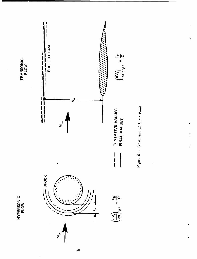
zuii

z iIi<i LIL

*

ZZ.J

IiiIiL

IiI

8 48

20.0 yoo = 7.20

7.10

18.0 7

7.02

16.0 7

6.9814.0 6

7.0012.0

> "

10.0 6.90

8.0 6.50

NACA 0015 AIRFOIL

MW = 0.729

6.0 a = 40

so = 0.0484035

6.004.0

2.0 I I I 1

0.010 0.015 0.020 0.025 0.030 0.035

x

Figure 7a - Varying with Outermost Boundary Location

Figure 7 - Velocity Gradients near Sonic Point

49

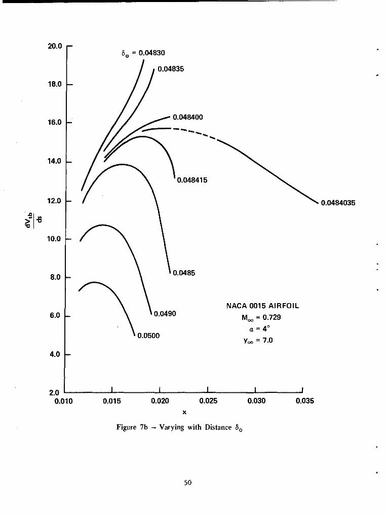
20.0 - s 0.04830

0.04835

18.0 0

16.0 - 0.048400

14.0 -

0.048415

12.0 0.0484035

10.0 -

8.0 - 0.0485

NACA 0015 AIRFOIL6.0 - 0.0490 Moo = 0.729

a = 400.0500 = 7.0

4.0 -

2.0 I I I I

0.010 0.015 0.020 0.025 0.030 0.035

x

Figure 7b - Varying with Distance 60

50

w

I-z0

w

o,, -J .Z..0 0< LL ':1:n

zn 0

00

cn 0

00

CL-

00

N 00

00

co 0-J

51

-00WcI~I6 0C.>8

a: C, zI, 8i

LO CC;o

LU >. a o0I Z .I I

ýc- LO0 ON

C icc N,

I 5C,,L I C

Ci .m

I~.4

6q

Cý oo

c;0

52

jLL.

r0 8IC

w 00

cno

C.,0

icr

I 05

ac ýe. u 11

4W ;

LO~

I NI

ID *

Nz 0

I-U I-

p dn

53

-0 C-D >o

(n~wI

C.,

I In

cnto

I 6

C)C.

U) I~Z I

Jw-ui 01

N. 0U. w

I-J w

54j

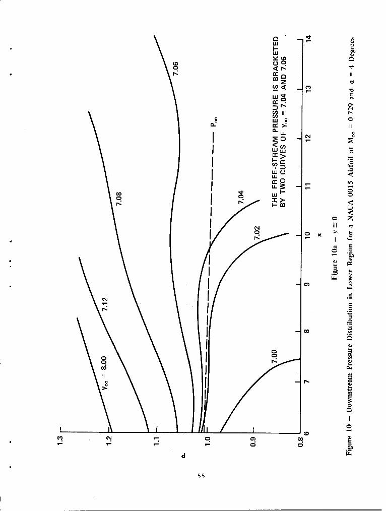
t ~I-

8 u0I80 -LL N 8

I ~ 0

0c 0 W 0

-0 X

* I*

* I 0c o

Ci Ci N

I55

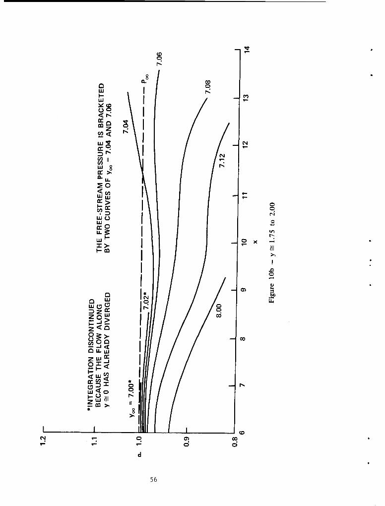
8000

lie

ccc

W C1

w8

ir Ia. U

IL L)

CdD

0

00

LI-

D 0

ig >. IfccOOD I

7LLW

zw~ d

F56

00:

K oqi..r.

ac

zcr.

I N

U.

<CdwLW U

CC >

ccc

0c 0

Lu

zccLu

0 cr.

IL -jd

crn*z

00

Z-U-LL

* 57

0 L0

0 0

0, Cio

0\ 0 0z z0, ,

(00

0L xz 0

w- It

U. 10N IU00 0~uu

ww I 6

0 t; 0

I>- w

No~ 0o Nd cs cs 6

580

w0 0

co r- iiw

ooco11A

Z 0 0 0

0 .1 .1 11 11

0000-j -

2200cc ir 0i:i0 a4a1

0w1 8

cl0zx

*uLUQ

A. u

w j z

a. J a

0 L0

> Iý

IN 00.)c

I-c d

d

59

ccoD6

00

o 0

0j 0

U hI 6

I 0~jW I

9LC

'ID

0 0 6s

w w a:

C.LLL

ww C,5 I

a-a- wd

600

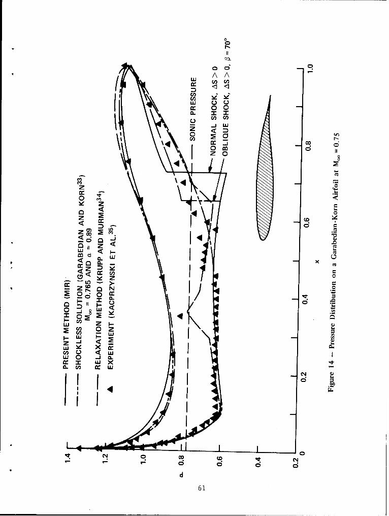
0

C00

A A

cr 0 0

0cc

zc

Z )C

Z <-

LI <cc z 4

LID >

0I 0 CCL-

02 0

~2 C)0 zo~I~ I// 6 3

0cc m0j

00 0 e

d

61

w

cc,

0 co

0 ~~

I- ~0ox

o tn

0 U0

0

w D

a'

Ito

zo 0

z x 10

00D~II

0 -j0II

IicoI

w 0

C5 03 dOC

62

00

L1*"

I J O

0 Dz

I..

z 0i

cojq <

D a.CL >

u

I- _I

w owLLL

cc wa. 0 z

636

REFERENCES

1. Tai, T.C., "Application of the Method of Integral Relations to

Transonic Airfoil Problems: Part I - Inviscid Supercritical Flow over

Symmetric Airfoil at Zero Angle of Attack," NSRDC 3424 (Sep 1970); also

presented as Paper 71-98, AIAA 9th Aerospace Sciences Meeting, New York,

N.Y. (Jan 1971).

2. Newman, P.A. and D.O. Allison, "An Annotated Bibliography on

Transonic Flow Theory," NASA TM X-2363 (Sep 1971).

3. Murman, E.M., "Computational Methods for Inviscid Transonic Flows

with Imbedded Shock Waves," Boeing Scientific Research Laboratories

Document Dl-82-1053 (1971); also presented in AGARD-VKI Lecture Series on

Numerical Methods in Fluid Dynamics, Rhode-Saint-Genese, Belgium (Mar 1971).

4. Norstrud, H., "A Review of Transonic Flow Theory," Lockheed-

Georgia Company, Report ER-11138(L) (Aug 1971); also presented as Paper

at University of Illinois Seminar (Mar 1971).

5. Yoshihara, H., "Some Recent Developments in Planar Inviscid

Transonic Airfoil Theory," AGARDograph 156, North Atlantic Treaty Organization

(Feb 1972).

6. Magnus, R. and H. Yoshihara," Inviscid Transonic Flow over Airfoils,"

General Dynamics/Convair Division Report (1969); also presented as Paper

70-47, AIAA 8th Aerospace Sciences Meeting, New York, N.Y. (1970).

7. Murman, E.M. and J.D. Cole, "Calculation of Plane Steady Transonic

Flows," AIAA J., Vol. 9, No. 1, (Jan 1971), pp. 121-141 (AIAA Paper No.

70-188, 1970).

8. Steger, J.L. and H. Lomax, "Numerical Calculation of Transonic

Flow About Two-Dimensional Airfoils by Relaxation Procedures," presented

as AIAA Paper 71-569 at AIAA 4th Fluid and Plasma Dynamics Conference,

Palo Alto, California (Jun 1971).

9. Holt, M. and B.S. Masson, "The Calculation of High Subsonic Flow

Past Bodies by the Method of Integral Relations," Second International

Conference on Numerical Methods in Fluid Dynamics, University of California,

64

Berkeley (Sep 1970).

10. Melnik, R.E. and D.C. Ives, "Subcritical Flows of Two-Dimensional

Airfoils by a Multistrip Method of Integral Relations," Second International

Conference on Numerical Methods in Fluid Dynamics, University of California,

Berkeley (Sep 1970).

11. Sato, J., "Application of Dorodnitsyn's Technique to Compressible

Two-Dimensional Airfoil Theories at Transonic Speeds," National Aerospace

Laboratory Technical Report TR-220T (Tokyo, Japan) (Oct 1970).

12. Emmons, H.W., "Flow of a Compressible Fluid past a Symmetrical

Airfoil in a Wind Tunnel and Free Air," NASA TN 1746 (Nov 1948).

13. Sichel, M., "Structure of Weak Non-Hugoniot Shocks," Physics of

Fluids, Vol. 6, No. 5, pp. 653-662 (May 1963).

14. Ferrari, C. and F.G. Tricomi, "Transonic Aerodynamics," Translated

by R.H. Cramer, Academic Press (1968).

15. Sinnot, C.S., "On the Prediction of Mixed Subsonic/Supersonic

Pressure Distributions," J. Aerospace Sciences, Vol. 27, pp. 767-778 (1960).

16. Nieuwland, G.Y., "Transonic Potential Flow around a Family of

Quasi-Elliptical Aerofoil Sections," National Aerospace Laboratory

(Amsterdam) Technical Report T-172 (Jul 1967).

17. Korn, D.G., "Computation of Shock-Free Transonic Flows for Airfoil

Design," New York University Courant Institute of Mathematical Sciences,

Report NYO-1480-125 (Oct 1969).

18. Boerstoel, J.W. and R. Uijlenhoet, "Lifting Airfoils with

Supercritical Shockless Flow," ICAS Paper 70-15, 7th Congress of the

International Council of the Aeronautical Sciences, Rome, Italy (Sep 1970).

19. Morawetz, C.S., "The Dirichlet Problem for the Tricomi Equation,"

Convn. Pure Appl. Math, Vol. 23, pp. 587-601 (Jul 1970).

20. Belotserkovskii, O.M. and P.I. Chushkin, "The Numerical Solution

of Problems in Gas Dynamics," in "Basic Developments in Fluid Dynamics,"

Vol. 1, edited by M. Holt, Academic Press (1965).

65

21. Chushkin, P.I., "Subsonic Flow of a Gas past Ellipses and

Ellipsoids," Translation of Vychislitel'naya Maternatika (USSR), No. 2,

pp. 20-44 (1957).

22. Chushkin, P.I., "Computation of Supersonic Flow of Gas past

Arbitrary Profiles and Bodies of Revolution (The Symmetric Case),"

Translation of Vychislitel'naya Maternatika (USSR), No. 3, pp. 99-110 (1958).

23. Tai, T.C., "Streamline Geometry and Equivalent Radius over a

Flat Delta Wing with Cylindrical Leading Edge at an Angle of Attack," NSRDC

Report 3675 (Oct 1971).

24. Ahlberg, J.H. et al., "The Theory of Splines and Their Applications,"

Academic Press (1967).

25. Klineberg, J.M., et al., "Theory of Exhaust-Plume/Boundary-Layer

Interactions at Supersonic Speeds," AIAA J., Vol. 10, No. 5, pp. 581-588

(May 1972).

26. Stivers, L.S., Jr., "Effects of Subsonic Mach Numbers of the

Forces and Pressure Distributions on Four NACA 64A-Series Airfoil Section

at Angles of Attack as High as 280,', NACA TN 3163 (Mar 1954).

27. Liepmann, H.W. and A. Roshko, "Elements of Gas Dynamics," Wiley,

N.Y. (1957).

28. Hayes, W.D., "Pseudotransonic Similitude and First Order Wave

Structure," J. Aero. Sci., Vol. 21, No. 11, pp. 721-730 (Nov 1954).

29. Pan, Y.S. and M.O. Varner, "Studies on Sonic Boom at High Mach

Numbers," AIAA Paper No. 72-652, presented at AIAA 5th Fluid and Plasma

Dynamics Conference, Boston (June 1972).

30. Graham, D.J., et al., "A Systematic Investigation of Pressure

Distribution at High Speeds over Five Representative NACA Low-Drag and

Conventional Airfoil Sections," NACA Report 832 (1945).

31. Spreiter, J.R. and A.Y. Alksne, "Thin Airfoil Theory Based on

Approximate Solution of the Transonic Flow Equation," NACA Report 1359 (1958),

Supersedes NACA TN 3970.

66

32. Pearcey, H.H., "The Aerodynamic Design of Section Shapes for

Swept Wings," in "Advances in Aeronautical Sciences," Pergamon Press, Inc.,

Vol. 3, pp. 277-322 (1961).

33. Garabedian, P.R. and D.G. Korn, "Numerical Design of Transonic

Airfoils," in "Numerical Solution of Partial Differential Equations,"

Academic Press, N.Y., Vol. 2, pp. 253-271 (1971).

34. Krupp, J.A. and E.M. Murman, "The Numerical Calculation of Steady

Transonic Flows Past Thin Lifting Airfoils and Slender Bodies," AIAA Paper

71-566 (1971), see also Boeing Scientific Research Laboratories Report

D180-12958-1 (Jun 1971).

35. Kacprzynski, J.J. et al., "Analysis of the Flow past a Shockless

Lifting Airfoil in Design and Off-Design Conditions," Nat'l. Res. Council

of Canada (Ottawa) Aero Report LR-554 (Nov 1971).

36. Lock, R.C., "Test Cases for Numerical Methods in Two-Dimensional

Transonic Flows," AGARD Report 575 (Nov 1970).

67

INITIAL DISTRIBUTION

Copies Copies

1 Chief of R&D (ABMDA) 10 NASA

I U.S. Army Missile Command 3 HQ, Washington, D.C.

3 CHONR 4 Ames Research Center

1 430B I Library

1 432 1 Dr. J.M. Klineberg

1 461 1 Dr. E. MurmanI Dr. J.L. Steger

1 USNA 2 Langley Research Center

I USNPGSCOL I LibraryI Mr. P.A. Newman

12 NAVAIRSYSCOM I Lewis Research Center

1 AIR 03AI AIR 03C 2 National Science Foundation1 AIR 310 1 Polytechnic Institute of Brooklyn3 AIR 320 Graduate Center Library1 AIR 5108 Long Island, N.Y. 117354 AIR 53012 AIR 604 1 Brown University

Division of Engineering2 NAVORDSYSCOM Providence, Rhode Island 02912

1 NADC 1 California Institute of Technology

1 NWC Pasadena, California 91109Attn: Graduate Aeronautical Labs.

4 NOL Aero. Librarian

1 Dept. of Aerodynamics 1 University of California

1 Dr. K.Y. Chien Berkeley, California 94720

1 Dr. A.H. Van Tuyl Attn: Dr. M. Holt, Div. of

1 Dr. T.F. Zien Aeronautical Sciences

1 University of CaliforniaI NWL Los Angeles, California 900241 NATC Attn: Dr. J.D. Cole

School of Engr. and Applied

I NAVMISCEN Sciences

I AFOSR 1 University of California

1 OAR, Holloman AFB La Jolla, California 92037Dept. of Aero. and Mechanical

I AF Inst of Technology Engineering Sciences

1 AEDC 1 University of Southern California

12 DDC Los Angeles, California 90007Attn: Dept. of Aerospace Engr.

68

Copies Copies

1 Catholic University of America 2 New York UniversityWashington, D.C. 20017 Courant Institute of Math. Sciences

1 University of Cincinnati New York, N.Y.

Cincinnati, Ohio 45221 Attn: Dr. P.R. Garabedian

Attn: Dept. of Aerospace Attn: Dr. D.G. Korn

Engineering 2 University of North Carolina

2 Clemson University Chapel Hill, N.C. 27514

Clemson, S.C. Attn: Dept. of Aero. EngineeringAttn: Library

1 Dr. T. Yang, Dept. of 2 North Carolina State UniversityMech. Engineering Raleigh, N.C. 27607

1 Library Attn: Dr. F.R. DeJarnette1 Cornell University Dept. of Mechanical and

Ithaca, N.Y. 14850 Aerospace EngineeringAttn: Graduate School of Attn: Library

Aero Engineering 1 Ohio State University

1 Georgia Institute of Technology Columbus, Ohio 43210Atlanta, Georgia 30332 1 Pennsylvania State UniversityAttn: Dr. Ben T. Zinn University Park, Penn. 16802

Aerospace Engr. Dept. Attn: Dept. of Aerospace Engr.

1 Harvard UniversityCambridge, Massachusetts 02138 Princeton UniversityLibaryPrinceton, N.J. 08540Attn: Gordon McKay Library Attn: Dept. of Aerospace and

1 Johns Hopkins University Mechanical SciencesBaltimore, Maryland 21218 1 Purdue University

1 University of Illinois Lafayette, Indiana 47907Urbana, Illinois 61801 Attn: Dept. of AeronauticalAttn: Aeronautical and Astro- Engr. and Astronautics

nautical Engr. Dept. 1 Stanford University

2 University of Maryland Stanford, California 94305College Park, Maryland 20740 Attn: Dr. J.R. SpreiterAttn: Dr. S.I. Pai, Institute Dept. of Applied Mechanics

for Fluid Dynamics and and Aeronautics andApplied Mathematics Astronautics

Attn: Library 2 University of Tennessee Space

1 Massachusetts Institute of Tech. Institute

Cambridge, Massachusetts 02139 Tullahoma, Tenn. 37388Attn: Dr. Y.S. Pan

1 University of Michigan Attn: Dr. J.M. WuAnn Arbor, Michigan 48104 2 University of Virginia

Attn: Library Charlottesville, Virginia 22901

1 New York University Attn: Alderman Library

University Heights Attn: Dept. of Aerospace Engr.New York, N.Y. 10453

69

Copies Copies

2 Virginia Polytechnic Institute I McDonnell Douglas Corporation

Blacksburg, Virginia 24061 Long Beach, CaliforniaAttn: Carol M. Newman Library Attn: Mr. A.M.O. Smith

Attn: Aerospace Engr. Dept. Nielsen Engineering and Research, Inc.

University of Washington Mountain View, CaliforniaSeattle, Washington 98105 1 North American Rockwell CorporationAttn: Dept. of Aeronautics Columbus, Ohio 43216

and Astronautics

I West Virginia University 1 Northrop Corporate LabsMorgantown, West Virginia 26506 Hawthorne, California 90250

Morgnton, est irgniaAttn: Dr. B.S. Masson

Attn: Dept. of Aerospace Engr.

1 TRW Systems Group

I Aerospace Research Laboratories Redondo Beach, California 90278

Dayton, Ohio Attn: Dr. D.R.S. Ko

I American Institute ofAeronautics and Astronautics

New York, N.Y. 10019 CENTER DISTRIBUTION

2 Boeing Company 25 1670

Seattle, Washington 98124Attn: Dr. R.C. GunnessAttn: Mr. A.S. Mahal

Cornell Aeronautical Lab, Inc.Buffalo, N.Y.Attn: Aerodynamics Research

Department

General Dynamics Corp.Fort Worth, Texas 76101Attn: Dr. F.K. Enseki

CONVAIR Division of GeneralDynamics Corp.

San Diego, California 92112Attn: Dr. H. Yoshihara

2 Grumman Aerospace Corp.Long Island, N.Y. 11714Attn: Dr. D.C. IvesAttn: Dr. R.E. Melnik

1 Institute for Defense Analyses

I Lockheed-Georgia CompanyMarietta, GeorgiaAttn: Dr. H. Norstrud

I LTV Aerospace CorporationVought Aeronautics DivisionDallas, Texas 75222

70

UNCTASSTFTEDSecurity Classification

DOCUMENT CONTROL DATA - R & D(Security classification of title, body of abstract and indexing annotation niust be entered when the overall report is classified)

I. ORIGINATING ACTIVITY (Corporate author) 12. REPORT SECURITY CLASSIFICATION

Aviation and Surface Effects Department UnclassifiedNaval Ship Research and Development Center 2b. GROUP

Bethesda, Maryland 200343. REPORT TITLE

APPLICATION OF THE METHOD OF INTEGRAL RELATIONS (MIR) TO TRANSONIC AIRFOIL PROBLEMS.PART II - INVISCID SUPERCRITICAL FLOW ABOUT LIFTING AIRFOILS WITH EMBEDDED SHOCK WAVE

4. DESCRIPTIVE NOTES (T),pe of report and inclusive dates)

Research and Development Report5. AU THOR(S) (First name, middle initial, last name)

Tsze C. Tai

6. REPORT DATE 7a. TOTAL NO. OF PAGES 17b. NO. OF REFS

July 1972 71 368a. CONTRACT OR GRANT NO. 9a. ORIGINATOR'S REPORT NUMBER(S)

NAVAIR TASK R230.201 NSRDC Report 3424b. PROJECT NO. Part II

C. NSRDC 1670-277 9b. OTHER REPORT NO(S) (Any other numbers that may be assignedthis report)

d. Aero Report 1176

10. DISTRIBUTION STATEMENT

Approved for public release; distribution unlimited

It. SUPPLEMENTARY NOTES 12. SPONSORING MILITARY ACTIVITY

Commander

Naval Air Systems Command (AIR-320)_ Washington, D. C. 20360

13. ABSTRACT

Numerical procedures developed in Part I of the present report for applyingthe method of integral relations to transonic airfoil problems are extended here tolifting cases. A modification of the strip arrangement described in Part I nowenables any desired number of strips and size of integration domain to be used. Thefull inviscid flow equations (may be rotational) are employed and approximated bysecond-order polynomials in transverse direction in a physical plane. Numericalprocedures including iterative processes for solving subject two-point boundaryvalue problems are formulated for the case of high subsonic free-stream Mach num-bers. Cartesian coordinates are employed except near the leading edge region wherethe use of a body coordinate system is convenient to account properly for largeslope variation there. The geometry of the airfoil is represented by cubic splinefunctions when a closed airfoil relation is not available. The effect of changeof entropy across the embedded shock wave is examined by allowing a decrease intotal pressure after the shock wave along the surface streamline. With the shockangle as a free parameter, oblique shock relations as well as normal shock relationscan be incorporated in the solution.

Results are presented for supercritical flows past various airfoils, includingtwo conventional, one advanced, and two shockless airfoils. Comparisons of theresults with existing theoretical and/or experimental data indicate reasonablygood agreements. It is found that the shock location moves forward in the case ofa finite increase in entropy across the shock wave; the entropy has, therefore, a

cumulative effect on the flow.

DD °OR ..1473 (PAGE 1) UNCLASSIFIEDS/N 0101-807.6801 Security Classification

UNCLASSIFIEDSecurity Classification

14. LINK A LINK 1 LINK CKEY WORDS

ROLE WT ROLE WT ROLE WT

Integral Relations

Lifting Airfoils

Inviscid Flows

Supercritical Flow

Subcritical Flow

Nonisentropic Flow

Normal Shock

Oblique Shock

Spline Function

FORM (AK

DDI Nov68 14 73 UNCLASSIFIED(P AGE- 2) Security Classification