naval postgraduate school monterey, california...b. testmethods 42 1. modalsurvey 43 2....
TRANSCRIPT
NAVAL POSTGRADUATE SCHOOLMONTEREY, CALIFORNIA
THESIS
AN ANALYSIS OF SPACECRAFT DYNAMICTESTING AT THE VEHICLE LEVEL
by
Alan D. Scott
June, 1996
Thesis Advisor: BrijN. Agrawal
ThesisS37565
Approved for Public Release; distribution is unlimited

DUDLEY KNOX LIBRARYNAVAL POSTGRAD' fATE SCMnniMONTEREY CA MiSi^r^

REPORT DOCUMENTATION PAGE Form Approved OMB No. 0704-0188
Public reporting burden for this collection of information is estimated to average 1 hour per response, including the time for reviewing instruction, searching
existing data sources, gathering and maintaining the data needed, and completing and reviewing the collection of information. Send comments regarding this
burden estimate or any other aspect of this collection of information, including suggestions for reducing this burden, to Washington Headquarters Services,
Directorate for Information Operations and Reports, 1215 Jefferson Davis Highway, Suite 1204, Arlington, VA 22202-4302, and to the Office of Management
and Budget, Paperwork Reduction Project (0704-0188) Washington DC 20503.
T. AGENCY USE ONLY (Leave blank) 2. REPORT DATEJune 1996
3. REPORT TYPE AND DATES COVEREDMaster's Thesis
4. TITLE AND SUBTITLE AN ANALYSIS OF SPACECRAFTDYNAMIC TESTING AT THE VEHICLE LEVEL
5. FUNDING NUMBERS
6. AUTHOR(S) Scott, Alan D.
PERFORMING ORGANIZATION NAME(S) AND ADDRESS(ES)Naval Postgraduate School
Monterey CA 93943-5000
8. PERFORMINGORGANIZATIONREPORT NUMBER
9. SPONSORING/MONITORING AGENCY NAME(S) AND ADDRESS(ES) 10.SPONSORING /MONITORINGAGENCY REPORT NUMBER
11. SUPPLEMENTARY NOTES The views expressed in this thesis are those of the author and do not
reflect the official policy or position of the Department of Defense or the U.S. Government.
12a. DISTRIBUTION/AVAILABILITY STATEMENTApproved for public release; distribution is unlimited.
12b. DISTRIBUTION CODE
13. ABSTRACT (maximum 200 words)
The US space industry has accumulated a vast amount of expertise in the testing of spacecraft to
ensure these vehicles can endure the harsh environments associated with launch and on-orbit
operations. Even with this corporate experience, there remains a wide variation in the techniques
utilized to test spacecraft during the development and manufacturing process, particularly withregard to spacecraft level dynamics testing. This study investigates the effectiveness of sinusoidal
vibration, random vibration, acoustic noise and transient methods of spacecraft dynamic testing. Ananalysis of test failure and on-orbit performance data for acceptance testing indicates that the
acoustic test is the most perceptive workmanship screen at the vehicle level and that additional
dynamics tests do not result in an increase in acceptance test effectiveness. For spacecraft
qualification, acoustic testing is almost universally employed for qualification in the high frequency
environment. For the low frequency environment, data collected from a variety of spacecraft test
programs employing sinusoidal sweep, random vibration and transient testing methods shows that a
transient base excitation provides the most accurate simulation for the purpose of designverification. Furthermore, data shows that sinusoidal vibration testing provides an unrealistic
simulation of the flight environment and results in an increased potential for overtesting.
14. SUBJECT TERMS Dynamics testing, vibration testing, spacecraft testing,
test effectiveness
15. NUMBER OFPAGES 136
16. PRICE CODE
17. SECURITYCLASSIFICATION OFREPORTUnclassified
18. SECURITYCLASSIFICATION OFTHIS PAGEUnclassified
19. SECURITYCLASSIFICATION OFABSTRACTUnclassified
20. LIMITATION OFABSTRACTUL
NSN 7540-01-280-5500 Standard Form 298 (Rev. 2-89)
Prescribed by ANSI Std. 239-18 298-102

11

Approved for public release; distribution is unlimited
AN ANALYSIS OF SPACECRAFT DYNAMIC
TESTING AT THE VEHICLE LEVEL
Alan D. !$cott
Commander, United States NavyB.S., United States Naval Academy, 1981
Submitted in partial fulfillment of the
requirements for the degree of
AERONAUTICAL AND ASTRONAUTICAL ENGINEER
from the
NAVAL POSTGRADUATE SCHOOLJune 1996

/ f^-Jf */'JS

DUDLEY KNOX LIBRARYNAVAL POSTGRADUATE SCHOOLMONTEREY CA 93943-5101
ABSTRACT
The US space industry has accumulated a vast amount of expertise in the testing of
spacecraft to ensure these vehicles can endure the harsh environments associated with
launch and on-orbit operations. Even with this corporate experience, there remains a wide
variation in the techniques utilized to test spacecraft during the development and
manufacturing process, particularly with regard to spacecraft level dynamics testing. This
study investigates the effectiveness of sinusoidal vibration, random vibration, acoustic
noise and transient methods of spacecraft dynamic testing. An analysis of test failure and
on-orbit performance data for acceptance testing indicates that the acoustic test is the most
perceptive workmanship screen at the vehicle level and that additional dynamics tests do not
result in an increase in acceptance test effectiveness. For spacecraft qualification, acoustic
testing is almost universally employed for qualification in the high frequency environment.
For the low frequency environment, data collected from a variety of spacecraft test
programs employing sinusoidal sweep, random vibration and transient testing methods
shows that a transient base excitation provides the most accurate simulation for the purpose
of design verification. Furthermore, data shows that sinusoidal vibration testing provides
an unrealistic simulation of the flight environment and results in an increased potential for
overtesting.

VI

TABLE OF CONTENTS
I. INTRODUCTION 1
II. SPACECRAFT DEVELOPMENT AND TESTING PROCESS 3
A. SPACECRAFT DEVELOPMENT AND TEST FLOW 3
1
.
Development Phase 3
2 . Qualification and Protoqualification Phase 3
3 . Acceptance Phase 44 . Prelaunch Validation Phase 5
B. SPACECRAFT ASSEMBLY LEVELS 5
1. Part Level 5
2. Unit Level 63 . Subsystem Level 6
4 . Vehicle Level 7
C. SPACECRAFT TEST TYPES 7
1
.
Functional Tests 8
2 . Thermal Tests 8
3 . Dynamics Tests 8
4 . Miscellaneous Tests 12
III. FUNDAMENTALS OF VIBRATION 13
A. RESPONSE OF A SINGLE DEGREE OF FREEDOM SYSTEM 13
B. MULTIPLE DEGREE OF FREEDOM SYSTEMS 18
C. RANDOM AND ACOUSTIC VIBRATION 22
D. SHOCK 25
IV. SPACECRAFT VEHICLE LEVEL DYNAMICS TESTING 31
A. TESTING AND THE LAUNCH ENVIRONMENT 31
1. Test Intent 31
2 . The Launch Environment 32a. Low Frequency Sinusoidal Environment 32b . Acoustic Vibration Environment 34c. Random Vibration Environment 35d . Shock Environment 37
3 . Specific Launch Vehicle Environments 38a. Deltal 38b. STS 42c. Adas 42
vn

B. TEST METHODS 421
.
Modal Survey 432 . Acoustic Vibration 433 . Random Vibration 444. Sinusoidal Vibration 44
a. Fundamentals 44b . Notching 45
5. Shock 466 Transient „ 47
C. TEST EQUIVALENCE 501
.
Sinusoidal and Random Vibration Equivalence 502 . Test Duration Relationships 52
V. VIBRATION TESTING ANALYSIS 55
A. TEST PHILOSOPHIES 551
.
Department of Defense 552. NASA 573 . Jet Propulsion Laboratory 584 . Commercial .59
B. TEST EFFECTIVENESS 591
.
Acceptance 60a. Criteria 60b . Data Analysis 62c. Survey Results 65
d . Experimental Results 672. Qualification 72
a. Criteria 72b. Study Results 74
VI. CONCLUSIONS AND RECOMMENDATIONS 103
A. CONCLUSIONS 103
1
.
Acceptance Testing 1032 . Qualification Testing 103
B. RECOMMENDATIONS 104
APPENDIX A. TYPICAL LAUNCH ENVIRONMENT SPECIFICATIONS 107
LIST OF REFERENCES 115
BIBILIOGRAPHY 119
INITIAL DISTRIBUTION LIST 121
Vlll

LIST OF FIGURES
1 .
1
DOD Spacecraft Testing Process 10
1 .2 GOES Spacecraft Testing Process 11
3 .
1
Single Degree of Freedom Mechanical System 14
3 .2 Response Factor versus Frequency Ratio 15
3.3 Transmissibility Versus Frequency Ratio 16
3 .4 Estimation of Quality Factor From Transmissibility Curve 17
3 . 5 Relative Response versus Sweep Parameter 19
3.6 Multiple Degree of Freedom Mechanical System 19
3 .7 Uniform Beam With Distributed Parameters , 21
3 . 8 Gaussian Distribution of Random Vibration 223.9 Rayleigh Distribution of Peak Accelerations 243.10 Power Spectral Density versus Frequency 243.11 Two Dimensional Shock Response Spectrum 263.12 Three Dimensional Shock Response Spectrum 273.13 Typical Shock Inputs 283.14 Shock Responses for Typical Shock Inputs 294. 1 Launch Load Spectrum 334.2 Typical Sound Pressure Level Plot 354.3 Typical Power Spectral Density Plot 364.4 Shock Response Spectrum Determination 384.5 MECO-POGO Thrust Axis Time History for Delta 1 404.6 MECO-POGO Thrust Axis Shock Response for Delta 1 414.7 Typical Notched Input and Corresponding Response 474.8 Derivation of Galileo Input and Response Pulses 495.1 "Roller Coaster" Failure Rate Curve 61
5 .2 Workmanship Experiment Failure Data 705.3 Transient Test Input 765 .4 Shock Response Spectrum Input 775 . 5 Comparison of ResponseMagnitudes for Notching Criteria B 785 .6 Comparison of ResponseMagnitudes for Notching Criteria C 795 . 7 Comparison of ResponseMagnitudes for Notching Criteria D 805 . 8 Comparison of Bending Moments for Notching Criteria B 81
5 .9 Comparison of Bending Moments for Notching Criteria C 825.10 Comparison of Bending Moments for Notching Criteria D 835.11 Notching Criteria 845.12 Swept Sine Test and Flight Levels 865.13 Transient Test and Flight Levels 865.14 Synthesized Waveform Test and Flight Levels 875.15 Number of Acceleration Peaks versus Amplitude 875.16 RMS Acceleration as a Function of Time 885.17 RMS Acceleration as a Function of Frequency 885.18 Cumulative Amplitude Histogram for Sinusoidal Sweep Tests 905.19 Cumulative Amplitude Histogram for Random Dwell Tests 915.20 Cumulative Amplitude Histogram for Transient Tests 925.21 Model Used for Galileo RTG Tests 955.22 Flight Shock Response Spectrum from Intelsat V Satellite Adapter 995.23 MAVIS Test Transient Response Data 101
IX


LIST OF TABLES
3 . 1 Probability Intervals 23
4.1 COBE/Delta I Flight and Test Response Levels 41
5 .
1
Governmental Agency Spacecraft Dynamic Test Requirements 565.2 Dynamic Test and Flight Failure Data 635.3 Workmanship Test Effectiveness Survey 665.4 JPL Workmanship Experiment Results 695.5 Topaz II Sinusoidal Vibration Test Inputs 71
5 .6 Topaz II Random Vibration Test Inputs 725.7 Topaz II Sinusoidal and Random Vibration Test Comparison 735 . 8 Comparative Response Amplitudes for Swept Sinusoidal, Random Dwell
and Transient Inputs 935.9 Response of a SDOF System to Sinusoidal Dwell, Sinusoidal Sweep
and Modulated Sine Pulse 965.10 Number of Response Cycles for a SDOF System with Sinusoidal Dwell,
Sinusoidal Sweep and Modulated Sine Pulse Inputs 965.11 Intelsat V Shock Spectrum Response Data 98
XI

Xll

ACKNOWLEDGMENTS
This thesis could not have been completed without the help and guidance of many
people. While it is difficult to acknowledge everyone who made a contribution to this
effort, there are several who deserve special recognition. First, I would like to thank
Professor Brij Agrawal, my advisor for this project, for allowing me to explore an area of
personal interest and to develop a foundation of knowledge which will hopefully be of
great benefit in future assignments. Professor Agrawal's expertise in spacecraft
engineering has been invaluable, not only for this thesis, but for several other projects
throughout the course of my graduate education.
I would also like to extend my deepest appreciation to Bill Tosney at the Aerospace
Corporation, who donated his time, his office, his data and many other resources. Without
Bill's considerable help, this thesis would not have been possible. In addition, Dennis
Kern of the Jet Propulsion Laboratory provided much valuable information on current JPL
research regarding spacecraft dynamic testing. I also wish to thank Professor Barry
Leonard for taking on the task of second reader with less than optimal warning. Also, I
owe a debt of gratitude to Mr. Tom Boyd of the Space and Naval Warfare Systems
Command and to Mr. Ed Senasack of the Naval Center for Space Technology for their
inspiration and support.
Finally, I would like to thank my family for their support over the years, especially
my parents, who taught me the value of education, and my sweetheart Marline, who stuck
by me through the ups and downs of the last two years.
Xlll


I. INTRODUCTION
Over almost four decades of space experience, the United States has successfully
developed, tested and launched hundreds of spacecraft. Throughout this period, the US space
industry has collected a significant amount of expertise in the most effective techniques for testing
space vehicles to ensure they are able to withstand the harsh environments associated with launch
and on-orbit operations. Even with this vast amount of corporate experience, there remains a wide
variation in the techniques utilized to test spacecraft during the development and manufacturing
process. Considerable differences exist among the many government agencies and corporations
involved in the US space industry in not only the types and quantities of tests performed but also
the severity of those tests. As testing costs can consume up to 35% of a space program's overall
budget, the amount of testing performed is of significant impact to overall program cost.
Likewise, proper levels of testing are extremely important for program success. If testing is not
severe enough, the probability of on-orbit failures is increased; too severe and the space vehicle
can be damaged before it is ever launched.
One of the specific areas in which this difference between test approaches is particularly
evident is in the realm of spacecraft dynamics testing. Different approaches to dynamic testing of
spacecraft at the vehicle level exist not only between NASA and Department Of Defense (DOD)
satellite programs but also between the many commercial participants in the US space industry.
One example of these differences is the utilization of low frequency sinusoidal vibration testing for
spacecraft qualification and acceptance. While many commercial and government space programs
include sinusoidal vibration testing as a regular part of the development, qualification and
acceptance process, others, including most DOD programs, do not. While the cost savings
associated with the deletion of sinusoidal vibration testing can be significant, the potential risks to a
program which does not adequately test a spacecraft prior to flight can be considerable.
The purpose of this thesis is to investigate the utility and effectiveness of the various
approaches to dynamics testing for both the acceptance and qualification of spacecraft at the system

level. The spacecraft development and testing process will be described and the various types of
spacecraft dynamic testing will be presented and compared. The underlying fundamentals of
vibration and the spacecraft dynamic environment will also be discussed. A survey will then be
conducted to determine the specific approaches to spacecraft dynamic testing currently in use
throughout the space industry. Test data from a variety of programs will be examined to determine
the effectiveness of these various approaches. Based on this analysis, an approach will be
recommended for dynamics testing of Department of Defense spacecraft.
II. SPACECRAFT DEVELOPMENT AND TESTING PROCESS
Because of the unique nature of space vehicles, the spacecraft development and testing
process is often long and complicated. As it is rarely possible to repair problems on orbit, space
vehicles must be designed and tested in a robust manner to minimize on-orbit failures. Though the
advent of Total Quality Management (TQM) has encouraged the improvement of design and
manufacturing processes, a vigorous test and verification program is still necessary to ensure
adequate on-orbit spacecraft performance. This test and verification program begins early in the
development cycle of a space vehicle and continues throughout the manufacturing, assembly and
launch process. While systems level dynamic testing is only one part of this overall development
and testing process, it is important to understand the entire process to determine the contribution of
dynamics testing to the successful production and launch of a spacecraft.
A . SPACECRAFT DEVELOPMENT AND TEST FLOW
1 . Development Phase
The spacecraft development and testing process generally begins with a development phase
during which the initial concept is formulated and design work is begun. During the development
phase, tests are performed to validate new design concepts, verify analytical models and reduce the
risk of transferring a design to actual flight hardware. These tests are often performed on special
developmental test articles or breadboard units which are not intended for flight and can therefore
be tested under more extreme conditions. Developmental tests are conducted to identify problems
early and according to the MIL-STD-1540C, "...confirm structural and performance margins,
manufacturability, testability, maintainability, reliability, life expectancy and compatibility with
system safety." [Ref. 1: p. 23]
2 . Qualification and Protoqualification Phase
Once the initial spacecraft design has been formulated and developmental testing has been
accomplished to verify design concepts and reduce the risk of new technologies, the development

effort generally enters a qualification or protoqualification phase. During this phase, a qualification
test article is built. The "qual" vehicle, which is as close to flight quality as possible, is subjected
to both functional and environmental tests to ensure that the design, materials and manufacturing
processes produce a spacecraft that meets mission specification requirements. The qualification
tests certify that both hardware and software work properly and that hardware can survive and
operate in the expected environment. Qualification tests also serve to verify analytical models
which have been developed to assist in the design verification process. In addition, qualification
tests validate the planned acceptance test program, including test techniques, procedures,
equipment, instrumentation and software.
To ensure adequate design margins, the qualification vehicle is generally exposed to test
levels higher than those expected in flight. Consequently, a spacecraft subjected to qualification
testing is generally not intended to be flown and is often utilized as a permanent test fixture.
However, to shorten the development cycle and reduce costs, a protoqualification or protoflight
approach is often taken. In this case the environmental test levels are lower than those used for the
traditional qualification and the qualification article is actually used for flight. When using this
approach, refurbishment of the test item may be necessary prior to flight.
3. Acceptance Phase
Once a spacecraft or component is qualified, other articles produced using the same design,
materials and manufacturing processes should also meet design specifications and are therefore
considered qualified for flight without being subject to qualification tests. However, because
materials and manufacturing processes are imperfect, some testing is required to "demonstrate
conformance to specification requirements and provide quality control assurance against
workmanship or material deficiencies." [Ref. 1: p. 72] Consequently, vehicles or components
produced after the qualification vehicle are generally subjected to acceptance tests to demonstrate
that the hardware is ready for flight. These acceptance tests are designed to stress items to
"precipitate incipient failures due to latent defects in parts, materials and workmanship" [Ref. 1 : p.
72] using test levels which are generally not as severe as those used for qualification.

4. Prelaunch Validation Phase
During the prelaunch validation phase, additional testing is accomplished to ensure
spacecraft readiness for launch. Such testing can be conducted both before and after shipping to
the launch site and is unique for each program depending on transportation methods and the launch
vehicle integration process.
Prelaunch operations can include functional testing, Reaction Control System (RCS) loading,
pressurization and checkout, ordnance system verification, launch vehicle mechanical and electrical
integration and verification, prelaunch countdown simulations and battery charging. Following the
successful completion of prelaunch validation activities, the spacecraft is launched and on orbit
checkout and operations begin.
B . SPACECRAFT ASSEMBLY LEVELS
The spacecraft development and testing process described above is executed at a variety of
levels. Development, qualification and acceptance tests are not only conducted on the entire
spacecraft after integration of all components, but each of the components and subsystems which
make up the spacecraft are also subjected to tests on an individual basis prior to installation on the
vehicle. As the test article becomes larger and more complex, the testing process becomes more
costly and difficult to perform and failures are often much more difficult to repair. Consequently,
the testing process is often tailored such that testing at the "lower" unit and component levels is
more comprehensive and severe than testing at the "higher" system level. This approach is
intended to detect and repair failures at the lower levels so that testing at higher levels can be
reduced. Because the type and quality of testing done at lower levels can have a significant impact
on the effectiveness of tests conducted at the system level, it is important to understand the testing
conducted at all levels.
1 . Part Level
In actuality, spacecraft testing begins at the part level, where individual parts such as
integrated circuits are screened to ensure they are manufactured properly and can withstand the

space environment. If part quality is low, tests at subsequent levels can have an abnormally high
failure rate. For DOD space programs, parts are generally required to conform to MIL-STD-
1546B, "Parts, Materials, and Processes Control Program for Space and Launch Vehicles," or
MIL-STD-1547B, "Electronic Parts, Materials, and Processes for Space and Launch Vehicles."
Commercial manufacturers typically invoke similar specifications for parts utilized on their
spacecraft. For the purposes of this study, it is assumed that adequate parts screening has been
conducted on all programs.
2. Unit Level
The unit level includes components such as electronics boxes, actuators, drive
motors and batteries which are "viewed as a complete and separate entity for purposes of
manufacturing, maintenance, or record keeping." [Ref. 1: p. 3] Unit level testing is conducted
during the developmental, qualification and acceptance phases of unit development and includes
both functional and environmental tests such as random vibration and thermal vacuum. Following
the successful completion of these tests, a unit is integrated either with a subsystem or directly with
the space vehicle for further tests. The type and quality of testing conducted at the unit level can
have a significant impact on test results at the subsystem and system level. DOD spacecraft
development programs generally conform to the requirements listed in MIL-STD-1540C for testing
at the unit level, while commercial manufacturers adhere to similar specifications. The impact of
unit level testing on the effectiveness of testing conducted at the system level will be discussed in
subsequent sections of this thesis.
3 . Subsystem Level
According to MIL-STD-1540C, "a subsystem is an assembly of functionally related units
[which] may include interconnection items such as cables or tubing, and the supporting structure to
which they are mounted." [Ref. 1: p. 3] While many units are integrated directly with the vehicle
and are tested together for the first time at the system level, some units are first integrated and
tested together at the subsystem level. Often, subsystems which have special test requirements and
which can be tested apart from the entire spacecraft are tested in this manner. A communications

payload, including associated antennas, is an example of a subsystem which might be tested in this
manner. While it is generally considered good practice to conduct tests at the lowest level possible,
unit level test requirements are sometimes fulfilled by testing performed at the subsystem level.
4 . Vehicle Level
Following the assembly of the spacecraft and integration of all units and subsystems, a
series of tests are generally conducted at the vehicle, or system level. These tests include both
functional and environmental tests and are intended to ensure that the entire vehicle meets either
qualification or acceptance requirements as appropriate for the phase of development. Because
many components of the spacecraft are integrated for the first time at the vehicle level, this testing
is critical in the detection of problems with such items as wire harnesses, connectors and plumbing
which cannot be completely tested at lower levels. In addition, while a high percentage of
manufacturing and materials defects are detected at the unit and subsystem level, it has been shown
that system level testing still exposes a significant number of unit level defects. [Ref. 2]
The types and order of tests performed at the vehicle level often vary depending on the
approach of the manufacturer or agency responsible for development of the spacecraft. As an
example, the typical vehicle level test flow for DOD spacecraft as specified in MTL-STD-1540C is
shown in Figure 1.1. This test flow specifies the performance of thermal cycle tests first, followed
by dynamics tests and then thermal vacuum tests. As a contrast, as shown in Figure 1.2, a vehicle
level test flow for the prototype Geostationary Operational Environmental Satellite (GOES) shows
dynamics tests followed by limited performance tests and thermal vacuum tests. The flight test
flow for a subsequent GOES vehicle thermal vacuum tests followed by dynamics tests. Thermal
cycling tests are not performed in either GOES test flow.
C. SPACECRAFT TEST TYPES
A variety of different tests are performed on a spacecraft and its components during the
different phases of development. Depending on program requirements, these tests may be
performed at the unit, subsystem or vehicle levels, and often may be repeated at all three levels.

These tests include functional tests, thermal and dynamics environment tests, and miscellaneous
tests.
1 . Functional Tests
Functional tests are intended to verify the mechanical and electrical performance of
components at the unit, subsystem and vehicle level. Functional tests are generally performed at
ambient temperature and pressure conditions prior to environmental tests to establish a performance
baseline. After the test article has been subjected to the required environments, additional
functional tests are conducted to determine the impact of the environments on the test article.
Functional tests are sometimes executed while a test article is being subjected to an environment,
but depending on the environment, this can be complicated and expensive, especially at the vehicle
level.
2. Thermal Tests
Thermal environment tests typically include thermal cycling at the unit level, thermal
vacuum tests at the unit and vehicle level and thermal balance testing at the vehicle level. Thermal
cycling and thermal vacuum tests are intended to verify performance of the test article in the
expected temperature and vacuum environments as well as to stress components to detect
workmanship and materials deficiencies. Thermal balance testing, on the other hand, is performed
to verify that the spacecraft thermal control system is able to maintain the vehicle and its
components within required operating temperature ranges when subjected to the thermal
environment of space.
3 . Dynamics Tests
Dynamics tests can include modal surveys, pyrotechnic shock, random vibration, acoustics
and sinusoidal vibration testing. Various combinations of these tests can be performed at the unit,
subsystem and system levels depending on the particular test program. Dynamics tests are
conducted during the development and qualification phases to verify that the spacecraft structure
and components can survive the expected dynamic environment, which is mostly a result of the
launch process. These qualification tests also are used to verify finite element models. Dynamics

tests are also conducted during the acceptance phase to stress components to detect workmanship
and materials deficiencies.
oBtO
70
SClO3
cr
soD
S 1
<
*- *
ofC/i
C38*
oooCO
-P".
5*
^ o» fP'W...
.
-*'; —-©•'-
33 _O =£ 3
3HS 9 . CO
n 0) I CO
panel
t
poin
loseo 2co
£[?«
T
OOOalibalibSE
3to
CDO -i -i-j- 0J <u "~
» CD CDtoCD
*- w 3" 3O f>D C/>
£3S oCD CD3 C/) CD**
CD"D CL
i r
T3 OCD 3- "03. CD cuo o <-i 7T
3 cooCO
CO _
CD X
CL
c"3Oj*
05 oCD 3
CO3CD
mot)O oC03 nim —
•
—
i
3« 3 ^,' Cfl
co c -<ca
COCO
<5 5'
< 3CO O
LOCL,_»><
T
:* >g« Co
3 3
3^ aCO
CO
coS- CD T3 ^o 3 T3 co
O 16
3 aCO
CD a T3CO Cl)
COCDto
o-1
3o
co
CD
V
?C 233 3 CQ CD mO £ 3"^, c-• o"~ COO ° CO O
to—
^
3 3i.- <T> c
CO S 3O
*< 3 o: 3c/ CO
ct
n
CD O Ofo M N)
b> to '-*
co
"D m m3 2 CO
to O o
1:2-"^worn
co |T'm."'©
*Cfl|
|.
.cu.
,^" :<
Figure 1.1. DOD Spacecraft Test Process. From Ref. [3].
10

c_>
LUIo
_J .
co >O £ 5 ,£a I < 5
lu O <
HO CO
IIIs
E 3oo
u. ll
CO -2 O< ztr. >1- CO
c-.
nc_>
LU
COoQ.
c
<2>-
^2- Lt
20<Ca.
o
z_| LU
< 2a -"oc
LUo u zP o
a. 0. _/
r5LU o <
" *
Soocv.
c
u VIBRATION
RATION
SH
OYMENT
St
o cj o yj£iO z LU LU
CM < CO CO Q
7o
o COLULU
UJo<
J (J n
z '-
u
L
• <LtLU Q LU
LCI
j2: trJO- LL
<o5 AL
MENT PROPMC/ES
MIC
IN
2o c
'. 0. oLU
UJ
LJ ^ CO LU£ O CO =
<7
CI a ll 3 < 2O < 2 uu
>O
1 I
cn
oo^?< 5mOI <Orr2 LU3 c< O
(71
<S
Lt I-
O 2LL LU
-2lu ;=tr -CL CO
"> Q S 07 ^ -t- LU ° p J?, LL
,_ CX CO — < ~O x 02gcr - o c-.
lu g ~
3o OT
PozH « ^ l7J o^5 - D<
< z(J LU
£„ 2
LU CO u r;
51luH°2£ < 2 lu < -
2fOC2H_j q. -j < < <lu O < 2 2 2
CO
<2J3£§— <>
LU JJ
o>< 00c 2
,,
O^crco uJ ir
1
k— — —co 2OOC- u
2O h-CT 2
^2C 2
LU O o 2 5
< 2
'OO-^cLU ° - ,7j LU
; s z 5 c£ CO -. < 2o = r 2gC — COuj 5
Figure 1.2. GOES Spacecraft Test Process. After Ref. [4].
11

Static testing also verifies the ability of the spacecraft structure to withstand the launch
environment. However, static testing is generally intended to verify only that the structure is able
to withstand the quasi-static forces of launch and does not provide verification for the dynamics
environment. In addition, the modal survey, which is generally performed on a structural test
model or qualification model vehicle to verify structural analytical models could also be considered
a dynamic test. These tests will all be described in detail in subsequent sections.
4 . Miscellaneous Tests
Additional tests which do not fit into the above categories include inspection, pressure and
leakage tests and electromagnetic compatibility (EMC) tests. These tests can be conducted
throughout the various phases of spacecraft development and at various levels of assembly. While
these tests can be important to the success of a spacecraft development program, they have little
impact with regard to dynamics testing and will not be considered in this study.
12
III. FUNDAMENTALS OF VIBRATION
The term vibration basically refers to oscillation in a mechanical system. This oscillation
can be defined by a frequency or frequencies and amplitude. The amplitude may be specified in
terms of displacement, velocity or acceleration. Sources of vibration can be deterministic,
following a specific pattern such as a sinusoid, or random. In addition, vibration can be free,
meaning that no energy is added to the system after an initial disturbance, or forced, meaning that
the system is continually disturbed by some input. In order to understand vibration testing, it is
important to understand the sources of vibration and their impacts on a mechanical system.
A. RESPONSE OF A SINGLE DEGREE OF FREEDOM SYSTEM
An understanding of the basic phenomena involved in dynamics testing of a spacecraft can
be gained by studying a simple single degree of freedom mechanical system. This system, as
shown in Figure 3.1, consists of a mass, spring and damper. We wish to define the motion of the
system in response to a continuing excitation, or forced vibration. The force may be applied to the
mass of the system or to the foundation that supports the system. For a sinusoidal force applied to
the mass in Figure 3. 1, the differential equation of motion is
mx" + ex' +kx = F sin (cot)
The steady state solution for the displacement of the mass can be placed in the form
x/xstatic = R sin (cot - 6)
where
xstatic = Fo/k
R = l/Kl-co^con2)2 + (25 co/cOn)2 ]
1/2
6 = arctan [(2 £ co/cOn)/(l - co^con2)]
£ = c/2mcon , and
con = (k/m) 1 /2
13

kp/
I
Figure 3.1. Single Degree of Freedom Mechanical System. From Ref. [5].
The dimensionless factor R, commonly called the displacement response factor or
magnification factor, provides the relative response of the maximum dynamic displacement to the
static displacement that would occur if the force F were applied statically. A plot of the response
factor R vs. co/u)n and C, is shown in Figure 3.2. Note that at G)/C0n = 1 the magnification factor is
limited only by the damping factor £. Without damping, the amplitude of the response is
theoretically infinite at resonance.
For the purposes of dynamic testing, we are interested in the amount of force transmitted
through the system, which can be defined by the ratio of the transmitted force to the applied force.
For a single degree of freedom system, the transmissibility is defined by
T = R[ l+(2£cfl/G)n)2 ]1/2
At resonance, when co/cOn = 1,
Tn = R[ 1+4£2 ]1/2 -
Note that for small damping the transmissibility and amplification factor are almost equal. Also, in
the forced vibration of a single degree of freedom system, the transmissibility is equal for either
mass excitation or base support excitation. Consequently, for a system being excited at its base,
such as a spacecraft attached to a launch vehicle, the response is similar.
14

«£ 6? «? n?
o.i 0.2 0.3 0.4
RATIO:
0.6 0.8 1.0 2
FORCING FREQUENCY
4 5 6 7 8910
UNDAMPED NATURAL FREQUENCY « r
Figure 3.2. Response factor Versus Frequency Ratio. From Ref. [5].
15

100
80
60
40
30
20
10
8
CD
to J
5 2cc
1.0
0.8
0.6
04
03
0.2
0.1
^C : 0.01
/C = 0.05
t\
L-C=0.10
1
Lc = 0.20
///
/
Jr Cr °" !>0
vN
\,A\u.iu 'y
?o0.50
0.01} ^_0.0 5 J
^ \0.1 0.2 0.3 0.4
RATIO
0.6 0.8 1.0 2 3
FORCING FREQUENCY _^NATURAL FREQUENCY " <"n
8 10
Figure 3.3. Transmissibility Versus Frequency Ratio. From Ref. [5].
16

Another quantity of interest is the quality factor for mechanical vibration, defined as
Q= 1/(2
At resonance, the magnification factor R is equal to the quality factor Q. Therefore, for systems
with small damping ratios, the transmissibility T and quality factor Q are approximately equal at
resonance. The damping of a system can be estimated from the transmissibility curve at resonance
by noting that the bandwidth of the curve at the half power points is Af = fn /Q, as shown in
Figure 3.4. Thus, to determine the damping, the transmissibility curve must be obtained by
experimental means. Otherwise, the damping must be estimated. [Refs. 5 and 6]
Figure 3.4. Estimation of Quality Factor from Transmissibility Curve. From Ref. [6].
For the purposes of dynamics testing, a swept sinusoidal input is often used as the forcing
function. The response spectrum for this swept sinusoidal input can be calculated from an
approximate formula. [Ref. 7] Given the steady state response of an excited system as
17
So(G)) = Q*L(co)
where L(co) is the input excitation, the relative response for a swept sinusoidal excitation can be
approximated by
So(co) = G*Q*L(co)
where
G=l-exp[-2.86i1 (-0.445)]
^ = P * q2 *in 2/(60 * f), and
P = the constant sweep rate in octaves/minute
Sweep rates are sometimes stated in terms of a sweep parameter, which includes the terms for
damping and natural frequency
sweep parameter = co' / (2 (?- ^hP")
where
co' = the sweep rate in rad/sec^
A plot of the relative response versus sweep parameter is shown in Figure 3.5. As would be
expected, the maximum response decreases as the sweep rate increases.
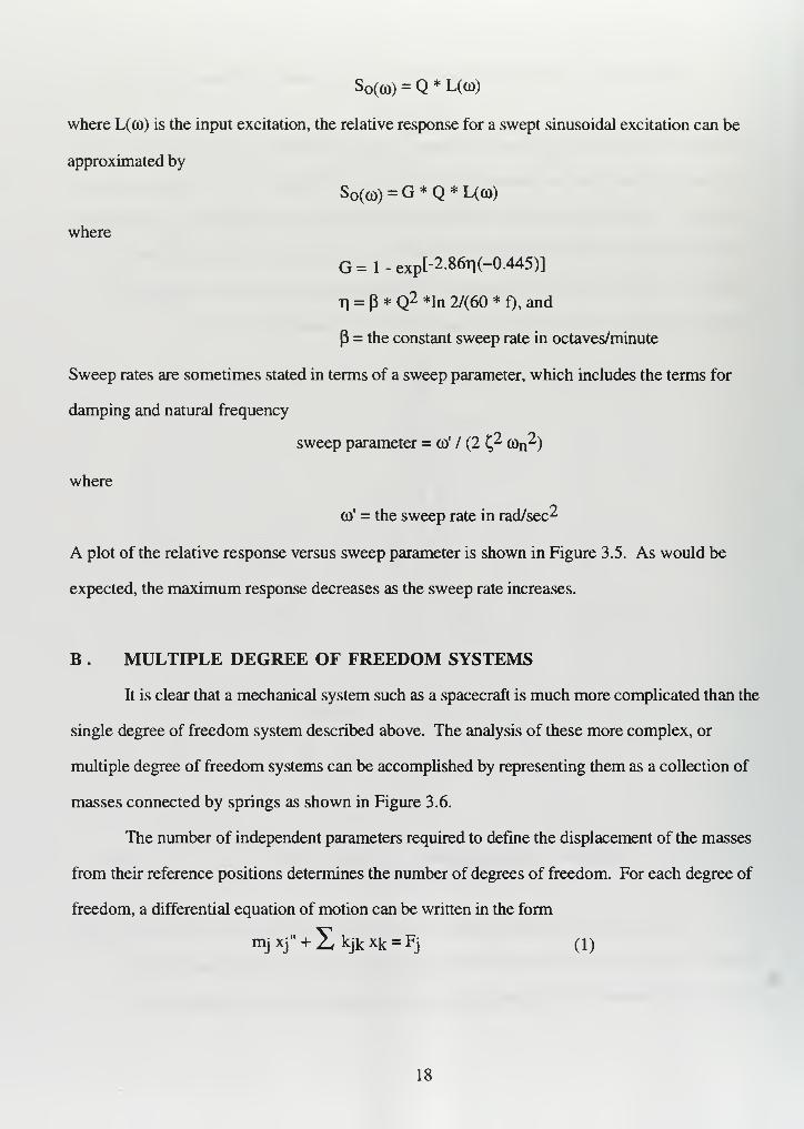
B . MULTIPLE DEGREE OF FREEDOM SYSTEMS
It is clear that a mechanical system such as a spacecraft is much more complicated than the
single degree of freedom system described above. The analysis of these more complex, or
multiple degree of freedom systems can be accomplished by representing them as a collection of
masses connected by springs as shown in Figure 3.6.
The number of independent parameters required to define the displacement of the masses
from their reference positions determines the number of degrees of freedom. For each degree of
freedom, a differential equation of motion can be written in the form
mjxj,, + Xkjkxk = Fj (1)
18

where
mj = the lumped mass of the jtri degree of freedom
kjk = the stiffness coefficient, and
Fj = the component in x direction of all external forces acting on the mass
f.O
.8
*SWEEP
'STEADY
.4
.2
125 25
x = AMPLITUDEX = DAMPING (c/c
r )
u = SWEEP RATEoj n
= NATURAL FREQUENCY
SWEEP PARAMETER, (J
2X u n NASA
Figure 3.5. Relative Response Versus Sweep Parameter. From Ref. [6].
rw^A/v* rwvw
Figure 3.6. Multiple Degree of Freedom Mechanical System. From Ref. [5].
19

For Fj = 0, this equation has solutions of the form
xj = Dj sin (cot + 9) (2)
Substituting this solution into the original equation results in
mjco2Dj = XkjkDk (3)
which is a set of n linear equations with n unknown values of D. A solution of these equations for
non-zero values ofD can be obtained only if the determinant of the coefficients ofD is zero.
(mio^-kii) -ki2
-k21 (m2C02 -k22)
-kiin
-kni (mn co2 - knn)
=
This solution provides the natural frequencies of the system, ©n, which are the frequencies
at which the system will oscillate in the absence of external forces. For each natural frequency,
there is an associated normal mode, or characteristic pattern of amplitude distribution. A normal
mode is defined by a set of values of Djn which satisfy equation (3) when co = con, or
con2 mj Djn =X kjn Dkn (4)
Another approach to the analysis of more complex mechanical systems is to apply the
principle of distributed parameters. A system with distributed parameters has an infinite number of
degrees of freedom and can be represented by an infinite number of masses and springs. Since the
number of natural frequencies of vibration of a system is equal to the number of degrees of
freedom, systems with distributed parameters have an infinite number of natural frequencies. As
with the previous analysis, a shape or normal mode is associated with each natural frequency. The
complete solution for the free vibration of the system would require the determination of all natural
frequencies and modes but in general it is necessary to know only the first few.
20

For analysis of the forced vibration of an elastic system with distributed parameters such as
a beam the classical approach is to apply Newton's second law to derive the equations of motion.
For a uniform beam as shown in Figure 3.7
EI 4y/3x4 ) + 7S/g(32y/at2) = F(x,t)
where
Which has the solution
where
E = modulus of elasticity
I = moment of inertia of the beam
y = weight density of the beam
S = area of cross section
yn = Ysn [l/O-co2/©!!2)] sin (cot)
ysn = ^Fg/oOn^Syl) (sin nrcx/1) (sin n7c/2)
So the amplitude of the n^1 term of the forced vibration is equal to the static deflection
under the Fourier component of the load multiplied by an amplification factor. "This is the same as
the relation that exists, for a system having a single degree of freedom, between the static
deflection under a load F and the amplitude under a fluctuating load F sin (cot)." [Ref. 5] As far as
each mode is concerned, the beam behaves like a single degree of freedom system. If the beam is
M +— dxdx
Figure 3.7. Uniform Beam With Distributed Parameters. From Ref. [5].
21

subject to a force fluctuating at a single frequency, the amplification factor is small except when
the frequency of the forcing function is near the natural frequency of a mode.
The results for a simply supported beam are typical of those which are obtained for
all systems having distributed mass and elasticity. Vibration of such a system at
resonance is excited by a force which fluctuates at the natural frequency of a mode.[Ref. 5]
C . RANDOM AND ACOUSTIC VIBRATION
For the analysis of the single degree of freedom system in Section A, the response was
specified assuming a deterministic, sinusoidal input. Random vibration, however, is non-
deterministic, meaning its instantaneous magnitude is predictable only on a probability basis. Such
vibration may be considered as being composed of a continuous spectrum of frequencies whose
individual amplitudes are varying in a random manner. The amplitude is described statistically by
determining the percentage of time the vibration is within certain limits. Random vibration is
considered to have a Gaussian or normal distribution as shown in Figure 3.8. The gaussian
distribution is described by the function
p(a) = l/[o-(27t) 1/2] exp(-a2/2a2)
where a is defined as the root mean square deviation, or standard deviation of the instantaneous
acceleration from the mean value. For random vibration, the mean is zero so a is simply the rms
;o 4-
Pla]
Figure 3.8. Gaussian Distribution of Random Vibration. From Ref. [6].
22

value of the instantaneous acceleration. For the curve shown in Figure 3.8, the probability that the
instantaneous value of the acceleration is between ai and a2 is equal to the shaded area under the
curve, or the integral of p(a) from ai to a2-
The vertical scale of Figure 3.8 is in dimensionless multiples of the rms value of the
vibration amplitude as defined by a. The probability, or percentage of time that a given value will
lie between the multiples of the rms amplitude (a) is shown in Table 3.1.
INTERVAL PERCENTAGE
-ato+a 68.27%
-2a to +2a 95.45%
-3a to +3a 99.73%
Table 3.1. Probability Intervals.
An equivalence between sinusoidal and random vibration can be established by conducting
an analysis of maximum damage potential as described in Chapter IV, Section C. For such an
analysis, peak values of acceleration are of more interest than instantaneous values. To describe
the peak value statistically, we consider a single frequency wave of randomly varying amplitude
which could be obtained if a random signal were passed through a narrow bandwidth filter. The
envelope of the peak accelerations for this narrow band random sinusoidal wave as shown in
Figure 3.9 is described by the Rayleigh distribution
p(ap) = (ap/a2) exp(-ap2/2a2)
Since the random vibration contains a continuous distribution of frequencies, all possible structural
resonances will be excited and the possibility of damage is much higher than with single frequency
sinusoidal vibration.
Random vibration is specified in terms of Power Spectral Density (PSD) in g2/Hz. As
shown in Figure 3.10, a plot of g2/Hz vs. frequency shows the power distribution or acceleration
23

One "Cycle"
p(Op)
Figure 3.9. Rayleigh Distribution of Peak Accelerations. From Ref. [6].
density of the vibration as a function of frequency. The overall mean square acceleration in g's
between frequencies f i and f2 is equal to the square root of the shaded area in the figure, or the
square root of the integral of the PSD from fi to f2- Random vibration which has a constant
acceleration density is called white noise and the mean square acceleration can be simplified to
grms = (PSDc *BW)i/2
where BW is the frequency bandwidth of interest.
PSO(£i)
f, f 2
f(Hz)
Figure 3.10. Power Spectral Density Versus Frequency. From Ref. [6].
24
Since all frequencies are present in the random vibration, a system with natural frequencies
within the band of interest will be excited at those frequencies by the corresponding single
frequency sinusoidal wave. The system responses will be continuous resonant responses with
transmissibility described by
T = Q= 1/(20
and the acceleration response at each resonant frequency will be
goutput = ginput * Q , or
g2/Hz = gi
2/Hz * Q2, or
PSD0Ut = PSDin*Q2
So, the PSD of the response at any frequency is equal to the input PSD multiplied by the square of
the transmissibility at that frequency.
For a constant or white noise input, the rms response can be calculated as (14):
grms = (rc/4£*fn*PSDn)l/2
where PSDn is the spectral density input to the system at the resonance frequency fn . Since at
resonance Q = 1/(2Q, we have
grms = [(rc/2)*fn*PSDn *Qn ]1/2 -
This expression provides the rms response of a simple system to white noise random vibration at
its resonant frequency. It is reasonably accurate for values of Q between 5 and 20 and in practice
is used for non-white vibration as well. [Ref. 6]
D. SHOCK
Mechanical shock is another significant part of the overall dynamics environment which a
spacecraft is required to withstand. While the focus of this study is on the comparison of
sinusoidal, random and acoustic vibration testing, it is important, to understand the fundamentals
of shock analysis and how shock testing fits in with other dynamics tests.
The response of a mechanical system to shock is typically expressed in terms of the shock
response spectrum (SRS). In a two dimensional shock response spectrum, the maximum value of
25

the response in a single time history is plotted as a function of frequency as shown in Figure 3.1 1.
This maximum response can be defined in terms of a displacement, velocity or acceleration. In a
three dimensional SRS, shown in Figure 3.12, the distribution of response peaks throughout a
time history is displayed as a surface. The two dimensional SRS is most typically employed for
shock testing.
14
12
I 10
2^ ft
O
t 6
Q-m rM-io/ v^o MUdpiei
Coupled Analysis
/N/K !St SpLimits
ec.
\ \
r \/ 'IN5s1,(X&XX
1
——i—
—
10 20 30 40 50 60 70 80 90 100
Frequency (Hz)
Figure 3.1 1. Two Dimensional Shock Response Spectrum. From Ref. [8].
Shock response analysis is usually based on the concept of the single degree of freedom
system as discussed in Chapter III, Section A. The excitation or input can be an impulse, step,
complex or other function in force, acceleration, velocity or displacement as shown in Figure 3.13.
The response can be determined analytically using classical differential equations, the Laplace
transform or convolution. Time histories and response spectrums for the shock inputs shown in
Figure 3.13 are shown in Figure 3.14. Both figures 3.13 and 3.14 are found in Reference 5.
26
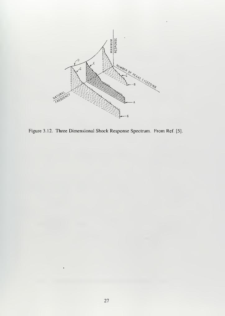
Figure 3.12. Three Dimensional Shock Response Spectrum. From Ref. [5].
27

TYPE Of ACCELERATION
SHOCK TIME-HISTORY
MOTION ii(T|
(A) IMPULSEu /<
lim
<-0
<
VELOCITY
TIME-HISTORY
utr)
"0
DISPLACEMENT
TIME -HISTORY
IB) STEP
IC) HALE-SINE u °
(0) DECAYING
SINUSOID w'u o
lt. = 0.ll
X2T/UJ, 1-
IE) COMPLEX 60°9l
4 8 12 16
Time. SEC <10
5
Figure 3.13. Typical Shock Inputs. From Ref. [5].
28

RELATIVE DISPLACEMENT RESPONSE & RESPONSE SPECTRUM A,,
ICI HALF- -fSINE ""
25. -CO-Ol-0.5" 10
/ALL f,
IMPULSIVE REGION
,c
Ol'.05 L_sunc PEGION
101 DECAYING «7SINUSOIO x/^^y "•^^''-
•
4>»'J- ".-,—Izr/uiU- w„.a
Ml9
/ v"^ /°'
s /-\/_Z°^>
(C^' 3 5*
5
"7
Ikx 05
= wn
50,
g
1/ N^O 1
1/ ^0
lOOOq
IEI COMPLEX
50Oo
i « 6 8 SECilO 1
[£ MJJ5CPSI
\l/\^AA/WVW-
2 « 6 8 SEC .10'
(5T I2J5 CPSI
500 q
2 A 6 3 SEC 10
'
Ijj "255 C?S)
^^C^o
025
000 2000 CPS
Figure 3.14. Shock Responses for Typical Shock Inputs. From Ref. [5].
29

30

IV. SPACECRAFT VEHICLE LEVEL DYNAMICS TESTING
A. TESTING AND THE LAUNCH ENVIRONMENT
1 . Test Intent
Dynamics testing of a spacecraft at the vehicle level is conducted for two primary purposes.
The first purpose is that of qualification: to ensure that the hardware can survive and operate in the
expected environment. For dynamics testing, this environment consists primarily of launch vehicle
induced loads as well as pyroshock from the deployment of mechanisms in flight. Other
contributors include ground transportation and handling, but these environments are typically less
severe and will not be discussed further.
For qualification, dynamic testing is only one part of the overall process employed to
ensure the space vehicle can withstand the dynamic environment. Another important part of the
process is the development of an analytical model of the vehicle structure. This analytical model is
uded to conduct a simulation to verify that the spacecraft design is adequate to survive the expected
dynamic loading. However, even when such a model is developed, testing needs to be performed
to verify the accuracy of the model. In addition, testing is also performed to ensure the design can
withstand environments which the analysis cannot accurately simulate.
The second purpose of dynamics testing is that of acceptance: to provide quality control
assurance against workmanship or material deficiencies. These workmanship or material
deficiencies are only problems if they result in the failure of the spacecraft to properly operate in the
operational environment. Consequently, for the exposure of material and workmanship problems,
the launch environment is again an important factor. Dynamics testing under launch conditions can
expose material and workmanship defects that might not be detected in a static condition but which
could occur in flight. [Ref. 1]
Two approaches can be used in the application of dynamic tests. The
first,environmental simulation, requires the reproduction of the exact mechanical environment to
which the vehicle is exposed during launch. While offering realism, this approach can be difficult
31

and expensive as it requires a close duplication of the various components of the launch
environment. The second, environmental equivalence, requires only that the environment applied
during testing has the equivalent effect of the actual launch environment. This approach can be
more simple as it allows flexibility in the way tests are conducted as long as the impact is the same.
However, it is often difficult to establish either analytically or experimentally whether a test
environment is truly equivalent. Equivalent test environments will be discussed in greater detail in
a later section.
2. The Launch Environment
The launch loads environment is made up of a combination of steady-state, low frequency
transient, higher-frequency vibroacoustic and very high frequency shock loads. A composite
sketch of these loads with their frequency and acceleration ranges is shown in Figure 4. 1. The
overall limit loads can be obtained by combining the root-sum-square (RSS) of the low and high-
frequency dynamic components with the steady state component. This results in the specification
of the launch limit loads typically published for particular launch vehicles. In addition to the limit
load specification, separate specifications for the low frequency transient and vibroacoustic
environments are usually provided. These environments are discussed in greater detail in the
following sections.
a. Low Frequency Sinusoidal Environment
The primary structural loads experienced by a spacecraft during launch usually
occur as a result of quasi-static loads due to acceleration or low frequency launch vehicle bending
modes. Launch vehicle modes of vibration which cause significant primary structural loads are
generally very low frequency modes, less than 20 Hz. Unless the spacecraft has resonant modes
in this frequency range, little dynamic coupling may be expected and the launch loads may be
considered as static loads criteria. [Ref. 9] These static loads are usually specified in terms of g
limits in the thrust and lateral axis.
For some launch vehicles, specific events such as Main Engine Cutoff (MECO) can
result in significant low frequency oscillations at the launch vehicle payload/interface. In these
32

Figure 4.1. Launch Load Spectrum. From Ref. [10].
cases, the low frequency environment is specified in addition to the static loads criteria.
Often referred to as the sinusoidal environment, this loading is typically expressed in terms of
acceleration amplitude in g over the frequency range of interest, which is usually under 200 Hz.
In addition to specific events such as MECO, low frequency oscillations can be
caused by certain launch vehicle phenomena such as POGO and chugging. POGO is a self excited
longitudinal vibration which is generated through the closed loop interaction of the launch vehicle
structure and propulsion system with combustion chamber pressure and thrust fluctuations.
According to Reference 11, POGO is an initially divergent longitudinal vibration which will be
stabilized and damped after 10 to 40 cycles. Typical POGO frequencies are 10 to 20 Hz for
booster stages, resulting in plus +/- 1 to 2 g output vibration levels at the payload.
During the thrust build up and decay of liquid rocket engines, periodic thrust
fluctuations may occur as a result of burning instabilities. Known as chugging, these fluctuations
can result in vibration in the range of 60 to 90 Hz for approximately 10 cycles.
33

b. Acoustic Vibration Environment
The principle sources of the acoustic environment include the interaction of rocket
motor exhaust with the surrounding air. This acoustic vibration is a function of rocket thrust, mass
flow rate and geometry and generally decays to a negligible level shortly after launch. The second
source of acoustic vibration is aerodynamic noise, which is a function of dynamic pressure, mach
number and vehicle geometry and is usually greatest in the region of maximum aerodynamic
pressure, or max Q. Consequently, the two periods of concern with regard to the acoustic
environment are liftoff and max Q.
Acoustic spectra are typically specified in terms of Sound Pressure Level (SPL) in
dB versus frequency as shown in Figure 4.2. The spectra are separated into octave band levels,
which are frequency bands in which the upper frequency is two times the lower freq. Occasionally
the acoustic environment is specified in 1/3 octave bands levels. In addition, an overall acoustic
level is generally specified. This level is the sum of the levels over the total frequency band of
interest.
Overall SPL (dB) =X 10 log [ 10 spKD + 10 SPK2) + ... 10 spl(n)]
The levels are expressed in terms of dB, defined as
dB=101og(P/Pref)2
where
P = pressure (rms), and
Pref = reference pressure = average hearing threshold
= 0.0002 u.bar = 2.9 x 10"9 psi (rms)
Acoustic vibration produces a high energy level over broad frequency range from
approximately 20 to 10,000 Hz. Acoustic energy is the primary forcing function causing higher
frequency vibrations of flight equipment such as secondary structure and components. In addition,
some equipment is sensitive to direct acoustic impingement. This includes items with high ratios
of surface area to mass (> 50 in^/lb) which are exposed to direct acoustic impingement such as
solar arrays and antennas. [Ref. 6]
34

145
135
125
-J 120ft
115 -
110
105 -
100
STS-l FLIGHT OATASTS-3 FLIGHT OATANASA MINIMUM TEST LEVELFOR EMPTY CARGO BAYPER NSTS 07700. VOL XIVATT. 1 (ICO 2-19001)
A/ \
• -/ -\ V
Cs
->—i—i—i—i—'—i—i—i
—
>—i—i ' i
125 250 500 1000 2000
1/3 OCTAVE BAND CENTER FREQUENCY (Hz)
—I ' '1 r
31.5 63 4000 8000
Figure 4.2. Typical Sound Pressure Level (SPL) Plot. From Ref. [12].
The acoustic environment is taken into account throughout the design and test of
units and subsystems. The establishment of appropriate vibration test levels at the component level
is an important factor in designing for the acoustic environment. Excessively conservative levels
can increase the probability of failure while excessively low levels can leave defects undetected.
Typical failures in electronic equipment include loose components, detached solder connections,
broken leads, cracked connectors and boards and damaged relays. Significant numbers of these
types of unit failures are often found in system level acoustic tests even though unit level tests
reveal most of the failures.
c . Random Vibration Environment
Random vibration in the launch environment is primarily produced through
structural transmission of acoustic pressures impinging on the surfaces of the vehicle. Other, less
35

significant sources include structure borne vibration transmitted directly from rocket motors and
other equipment. Because the random vibration environment is primarily a product of acoustic
noise, acoustic testing is often conducted instead of random vibration at the vehicle level.
However, as discussed in more detail in a later section, acoustic vibration does not excite the
structure as significantly at low frequencies.
Random vibration is usually quantified in terms of Power Spectral Density (PSD) in
g2/Hz. The PSD is equal to the mean square acceleration (g rms)2 level in a 1 Hz wide frequency
band versus the center frequency of that band. A typical plot of PSD versus frequency is shown in
Figure 4.3. The overall rms acceleration in g's may be determined from the PSD by integrating the
PSD over the desired frequency range
g (rms) = [jPSDdf ]1/2
"Random vibration environments are generally not design drivers for primary
structure." [Ref. 6] Because the higher frequency (>50 Hz) environments are usually acoustically
induced, the random environment mainly affects secondary structure and electronic and
electromechanical equipment.
0.04 q2 /Y\z
80 350
Frequency ~ Hz
3 dB/Octave
2000
Figure 4.3. Typical Power Spectral Density Plot. From Ref. [12].
36

d. Shock Environment
Mechanical shock is generated by a variety of events throughout the launch and
deployment of a spacecraft. These events include the separation of booster stages, the separation
of the payload from the booster and the release and deployment of stowables such as solar arrays
and antennas. In many of these events, pyrotechnic devices such as explosive bolts and nuts and
bolt cutters are employed. Consequently the shock environment is often referred to as pyrotechnic
shock or pyroshock. Typical shock environments range from hundreds to thousands of g's with
durations of 10 to 15 milliseconds.
As discussed previously, the shock response spectrum is the standard industry
method for displaying the relative severity of a transient event in the frequency domain. As shown
in Figure 4.4, the SRS indicates the maximum response of a simple mechanical oscillator when
subjected to the acceleration transient as a base input. The shock response spectrums are specified
for a particular value of Q, which is the amplification at resonance of a single degree of freedom
system
Q = response/input = l/2£
where
C, = % of critical damping
Thus, the percent of critical damping of the particular structure must be estimated or determined
experimentally.
Nearly all failures caused by pyroshock occur in electrical and electromechanical
units. Problems include the failure of relays and switches, breakage of leads, cracks in solder and
particle contamination. In fact, there are several examples of launch vehicle failures due to chatter
or transfer of relays. "Seldom will structure be affected, with the exception of small secondary
structural items that may be located in close proximity to an intense shock source such as a linear-
shaped charge separation device." [Ref. 13]
37

SHOCK TIME HISTORYRESPONSE
SERIES OF SIMPLE MECHANICAL OSCILLATORS
Cji i r
y^* i »! ^ ">n T^ T^^3 CZZD
, = -250Ri 500 Hi 1000 Hi 2000 Hi 4000 Hi S0O0 Hi
10 20MILLISECONDS 3000
b
12000 -
w
a iooo _
250 500 1000 2000 4000 *000
FREQUENCY (Hi)
Figure 4.4. Shock Response Spectrum Determination. From Ref. [6].
3 . Specific Launch Vehicle Environments
As discussed previously, a primary function of environmental testing is to ensure that
spacecraft hardware can survive and operate in the expected environment. Therefore, it is
important to have an understanding of the launch environments generated by various launch
vehicles. The following section provides a summary of the environments for several launch
vehicles and describes how these environments are determined. This information is intended to
provide a basic overview and is not intended to be a comprehensive discussion of the environments
for the given vehicles.
a. Delta I
The Delta launch vehicle is built in a variety of configurations. These
configurations differ in the type of engines used in the first and second stages, the type and number
of augmentation (solid rocket) motors and the presence and type of upper stage utilized. The Delta
I will be used for an example in this study as there was a significant amount of analysis conducted
on the low frequency environment for the NASA Cosmic Background Explorer (COBE) project.
38

The Delta launch environment, as specified in Reference 14, includes static load
factors, random vibration limit levels, acoustic levels and shock response spectra. The levels for
these various environments are provided in Appendix A. In addition, while Reference 13 does not
provide specific sinusoidal vibration requirements, it does state that, "There are periodic oscillatory
vibrations associated with several events (POGO) during the Delta launch. These occur at
frequencies below 50 Hz, and may be amplified by spacecraft dynamics. The need to perform a
sinusoidal vibration test to assure survival during these events must be assessed." [Ref. 14]
Indeed, for the COBE project, an in-depth analysis was conducted to determine the need for
sinusoidal vibration testing and to derive the test levels to be used.
As discussed in Reference 15, sustained periodic oscillation events were found to
occur on the Delta I. These events, which manifest themselves as sinusoidal inputs to the payload,
are called pre-MECO (Main Engine Cutoff) POGO, and MECO-POGO. Pre MECO POGO, also
commonly called mini-POGO occurs at a frequency of 27 Hz and again at 30-40 Hz while MECO-
POGO occurs between 15 and 21 Hz. According to Reference 15, the published sinusoidal sweep
test levels for the Delta I are generally conservative because they envelope a wide range of
spacecraft vehicle combinations. Consequently, the derivation for COBE was accomplished by
considering existing flight data from several previous Delta I missions as well as analytic
predictions from the COBE/Delta coupled loads analysis for the MECO-POGO and mini-POGO
events. "The sinusoidal levels were derived as a COBE unique set of levels. The sweep rate was
established so that the time spent sweeping through a particular frequency range during test was
approximately the same as the time duration of the event in flight." [Ref. 15: p. 234] The duration
ofMECO-POGO was about 5 sec which resulted in a 4 octave per minute sweep while the mini-
POGO duration was 10 sec which resulted in a sweep rate of 2 oct/min.
The sinusoidal vibration test magnitudes were established using the McDonnell
Douglas Astronautics Company (MDAC) coupled loads analysis along with a COBE project
analysis of flight data. The flight data included data tapes from 15 missions (14 flights of the 3920
series and one flight of the 3910 series). Shock response spectrum (SRS) plots were developed
39

from the time histories of launch accelerations obtained from accelerometers on the second stage
guidance section. A bandpass filter from 20-40 Hz was employed and SRS plots were generated.
A time history for the MECO-POGO event is shown in Figure 4.5 and the corresponding SRS plot
is shown Figure 4.6. The SRS plot was developed using a Q of 20, which was based on test data
from vibration testing on a COBE Engineering Test Unit (ETU). The SRS was divided by Q to
determine the appropriate sinusoidal test level. The flight level was defined as the mean plus 2
sigma and the protoflight test level was then established as 1 .25 times flight level.
2.0
1.5
^m. 1.0ma
0.5zoH 0.0<CUl-I
-0.5
UJoo -1.0
-1.5
-2JD
MlMMl illfrown!wpmil
U.O 0.5 1.0 1.5 2.0 2.5 3.0 3.5 4.0
TIME (SEC)
Figure 4.5. Delta 1 MECO-POGO Thrust Axis Time History. From Ref. [15].
The analysis of the flight data showed that the first mini-POGO occurred on all 15
missions. Test levels for this event were set at . 15 g's in the thrust direction and 0.50 g's in the
lateral direction. For the lateral direction, the level was determined as the root sum square of the
pitch and yaw levels. Conversely, only 5 of 15 missions showed the second mini-POGO . A
similar analysis resulted in a 0.14 g level in the thrust direction and 0.27 g's in the lateral direction
at a frequency of 31 to 33 Hz. For the actual COBE launch, all three events occurred but the levels
were lower than test levels as shown in Table 4. 1
.
40

35
<o
<3 30
Uia3 25>-
Z<T-t 21)aUICOz 15Oa.COUI 10cc
oo 5XCO
•
•
; Q = 20•
i
'
;
:
'
I,
; •
;-:
5 10 15 20 25 30 35 40 45 50
FREQ (Hz)
Figure 4.6. Delta 1 MECO-POGO Thrust Axis Shock Response. From Ref. [15].
FLIGHT EVENT/FREQUENCY
FLIGHT LEVEL(g's)
TEST LEVEL(g's)
TEST/FLIGHTRATIO
Thrust Axis
MECO-POGO (17.7 Hz) 1.60 2.20 1.38
Mini-POGO I (27.3 Hz) 0.08 0.15 1.88
Mini-POGO II (32.0 Hz) 0.004 0.15 37.50
Lateral Axis
MECO-POGO (17.7 Hz) 0.35 0.80 2.28
Mini-POGO I (27.3 Hz) 0.14 0.50 3.57
Mini-POGO II (32.0 Hz) 0.05 0.27 5.40
Table 4. 1. COBE/Delta I Flight and Test Response Levels.
41

b. STS
As specified in Reference 14, the environment for the Space Transportation System
(STS) or Space Shuttle includes structural loads and acoustic vibration. Structural loads are
determined on a case by case basis and acoustic levels are as specified in Appendix A. The
mechanical shock environment produced by the shuttle orbiter is considered negligible. In
addition, no sinusoidal requirements are specified for shuttle payloads.
c. Atlas
Like the Delta, the Adas comes in a variety of configurations. Versions of the Atlas
currently operational include the Atlas I, n, HA and HAS. The Atlas environment includes
specifications for limit load factor, acoustic levels, random vibration levels and shock response
spectrum. Environments for several versions of the Atlas are provided in Appendix A. While not
discussed in Reference 14, the Atlas environment does have a low-frequency quasi-sinusoidal
component. As specified in Reference 16, the Atlas II DOD User's Mission Planning Guide, the
flight measured low frequency vibration in the to 50 Hz spectrum does not exceed +/-1.0 g
axially or +/-0.7 g laterally. These peak responses occur for a few cycles during transient events
such as launch, gusts, Booster Engine Cutoff (BECO) and MECO. The Mission Planning Guide
recommends that if the spacecraft is tested at the vehicle level with a sinusoidal base vibration the
input levels should be tailored to frequency characteristics and response levels consistent with the
coupled loads analysis.
B . TEST METHODS
The following section provides an overview of the various dynamic tests employed in the
spacecraft development process. These tests can be performed for model verification, for
qualification of the vehicle in a particular environment or for workmanship and materials screening.
While some tests clearly correspond to a particular environment, others can be utilized to provide
equivalence to several environments.
42
1 . Modal Survey
Modal surveys are generally conducted during the development phase to verify that the
analytical model of the spacecraft adequately represents the structural dynamics of the actual
vehicle. The modal survey determines the natural frequencies and mode shapes of the structure in
addition to establishing a lower bound estimate for structural damping. Occasionally modal survey
data is used to experimentally derive the structural dynamic model of a vehicle, but this approach is
less common. [Ref. 17]
A variety of techniques can be used to conduct modal surveys. These include low level
sinusoidal dwell, sinusoidal sweep, random vibration or impact tests. The modal survey can
employ single point base or multi-point excitation and typically covers a frequency range from as
low as 3 Hz up to 100 Hz. As the goal is to excite the vehicle only enough to determine the natural
frequencies and mode shapes, input levels are much lower than those used for qualification or
acceptance testing. Once the analytical model is verified using the modal survey results, the
spacecraft model can be coupled with the launch vehicle model to obtain a final estimate of flight
loads. These flight loads are then used to establish the test levels for qualification and acceptance
of spacecraft hardware.
2 . Acoustic Vibration
Acoustic tests are often conducted at both the qualification and acceptance levels. The
qualification acoustic test demonstrates the ability of the vehicle to operate during and after
exposure to the extreme expected acoustic environment in flight. In addition, the qualification test
ensures that the level of acoustic testing for acceptance will not result in an over test of the flight
vehicle or vehicles. The acceptance acoustic test simulates the flight or minimum workmanship-
screen acoustic environment as well as the induced vibration on units in order to expose material
and workmanship defects that might not be detected in a static condition. [Ref. 1]
Vehicle level acoustic testing is generally conducted in a reverberation chamber with the
vehicle in a stowed configuration simulating conditions inside the payload fairing. As items such
as solar arrays and external antennas are especially susceptible to damage from acoustic vibration,
43

these components are either included in the vehicle level tests or are tested separately at the
subsystem level. Acoustic tests typically cover the range from 10 Hz to 10,000 Hz with sound
pressure levels from 120 to 145 dB depending on the specific environment and test phase.
3 . Random Vibration
Random vibration tests are sometimes conducted at the vehicle level instead of an acoustic
test for small, compact vehicles which can be excited more effectively via interface vibration than
by an acoustic field. In the case of MIL-STD-1540C, this includes vehicles under 400 lbs. For
larger vehicles, random vibration exerted at the launch vehicle/spacecraft interface does not
typically excite either primary or secondary structure adequately to simulate the acoustically
induced environment. Consequently, the acoustic test is typically specified for these larger
vehicles. When conducted, random vibration tests typically cover the frequency range from 20 Hz
to 2000 Hz at levels up to 0.05 g2/Hz.
A narrow band random dwell vibration test has been studied as an equivalent input for the
low frequency quasi-static environment. [Ref. 18] Tests were conducted using a 3 Hz bandwidth
signal with the input level raised until the critical locations monitored with accelerometers reached
the maximum predicted flight response level.
4 . Sinusoidal Vibration
a . Fundamentals
Sinusoidal vibration testing of spacecraft at the vehicle level is not consistently
employed throughout the space industry. Many manufacturers rely only on structural models for
design verification for the low frequency environment, especially below 20 Hz where models are
considered fairly accurate. In addition, it is often impractical to vibrate large spacecraft. When it is
conducted, sinusoidal vibration testing is usually justified for one or all of the following reasons
[Ref. 19]:
1 . Sinusoidal vibration provides an equivalent effect for the low frequency launch
transient environment which is a significant design driver for primary and
secondary structure as well as many assemblies and subsystems.
44

2 . Sinusoidal vibration is the only environmental test that dynamically excites the
lower frequency spacecraft response modes.
3 . Sinusoidal vibration provides the only significant dynamics workmanship and
design verification for most secondary structure and many assemblies and non-
structural system elements.
Sinusoidal vibration testing uses a slowly swept base input sinusoidal excitation to
excite system resonances to levels of response which simulate the levels expected to occur during
launch. The primary sources of launch excitation considered in developing the sinusoidal vibration
test specification are transients produced by events such as engine ignition, burnout and staging.
[Ref. 9] Typical sinusoidal vibration levels are in the range of 0. 1 to 2.0 g's at sweep rates of 2 to
8 Hz. However, studies have been conducted which employ fast swept sinusoidal inputs of up to
80 oct/min. [Ref. 7]
While the sinusoidal vibration test is considered simple to control and execute, the
test is generally very conservative and can result in significant over-test if not executed properly
[Ref. 20] For this reason many spacecraft development programs do not conduct sinusoidal
vibration testing. To reduce the potential for over-testing, current practice among programs which
conduct sinusoidal vibration testing is to employ a technique called notching.
b . Notching
As discussed previously, the low frequency transient environment is typically
defined in terms of the shock response spectrum (SRS). Because shock spectrum analysis does
not take into account the mechanical impedance of the test item, the characteristics of the spacecraft
do not influence the vibration test specification levels. In addition, the vibration test configuration
usually does not simulate the boundary conditions and mechanical impedance which the spacecraft
sees when it is attached to the launch vehicle. Finally, when subjecting a spacecraft to vibration in
a single axis, cross coupling may occur, producing excessive responses in another axis. The
overall result is that certain resonant modes of the spacecraft, usually the fundamental bending
modes, may be excited to levels of response during the vibration test which exceed the levels
45

actually observed during launch. This problem can be solved either by over designing the
spacecraft structure to handle these loads or to reduce the test level. Notching has become an
accepted method of achieving this reduction. [Ref 9]
Determination of appropriate sinusoidal vibration levels and associated notching
levels begins with the mathematical analysis of the vehicle. The mathematical model of the
spacecraft structure is coupled to a math model of the launch vehicle to perform launch loads
analysis. A complete launch loads analysis includes excitation of the launch vehicle math model
with a series of transients which represent each of the events known to result in primary structural
loads. A vibration test loads analysis is also done to determine response of the spacecraft structure
to the vibration test specification input. Since the sinusoidal input is swept very slowly, the
response of the spacecraft at its resonance frequency approaches steady-state conditions. The
response at resonance is dependent on the quality factor Q, which is a function of modal damping
as discussed previously. Therefore, assumptions regarding modal damping are critical in
calculating the response of each mode at resonance. [Ref. 9]
Following generation of the loads analyses, a comparison is made of the vibration
test loads with the launch loads to determine if notching is required. If the test response is greater
than that for the launch loads, the test input is reduced at the frequency of concern such that the
response matches the expected flight response. A typical notched input and corresponding
response is shown in Figure 4.7. Notch parameters are usually verified prior to the actual test by
conducting a low level sinusoidal sweep survey. Automatic control of sinusoidal sweep tests can
also be accomplished by switching the control parameter between input acceleration and response
acceleration when the response reaches the specified limit. [Ref. 91
5 . Shock
The shock test demonstrates the ability of the vehicle to withstand or operate in the induced
shock environment. This environment includes events such as solid rocket motor (SRM) and
payload fairing (PLF) separation as well as booster staging. In addition, the shock environment
includes the deployment of components such as solar panels which are initiated by explosive
46

ordnance or other devices, along with impacts and suddenly applied or released loads. [Ref. 1]
"Shock environments have caused more flight failures in past aerospace vehicle programs (1960-
1977) than vibration or acoustic environments." [Ref 6]
Units and subsystems are typically shock tested on vibration shakers or shock synthesizers
to levels of up to 3500 g. At the system level shock testing typically includes the firing of all
ordnance such as explosive nuts, bolts and pin pullers. This enables the definition of the shock
response spectra at various equipment locations. While system level ordnance firing is a good
simulation of the shock environment but does not demonstrate design margin.
1 25 i 20 00
£ 12 00 INPUT AMPLITUOE
NATURAL FREQUENCY = 8 00 Hi
FRACTION OF CRITICAL DAMPING = 02
SWEEP RATE IOCT/MINI = 2 00
COMPRESSION RATE IdB/secl = 2 000
OOJ 0000 20 60 80 1 00
FREQUENCY RATIO | ^ /„ |
ALLOWABLE RESPONSEAMPLITUOE
RESPONSE AMPLITUDE
120 1 40 1 60
Figure 4.7. Typical Notched Input and Corresponding Response. From Ref. [21].
6 . Transient
Until the advent of digital vibration control systems, low frequency dynamics testing was
restricted to swept sinusoidal and random vibration inputs. With the digital control systems,
transient waveform control became possible using fast fourier transform algorithms. As will be
discussed further in a later section, several studies have shown that a transient waveform test
derived from the shock response spectrum can reduce the potential of over test to secondary
47
structure. In addition, the transient approach can reduce the number of load cycles to which the
test article is exposed.
Transient testing can be conducted to simulate either the shock environment or the low
frequency transient and sinusoidal environment. Transient tests are typically conducted by
generating a base excitation corresponding to either a standard pulse or to the shock response
spectrum (SRS) of the transient of concern. For the input developed using the SRS, the transient
waveform with the desired shock spectrum can be synthesized from a pulse train of damped
sinusoidal wavelets. The main parameters in shaping the input SRS are the amplification factor Q
and the number of sinusoidal wavelets. Amplification factors of 10 (5% damping) to 20 (2.5%
damping) are typically used.
Variations in transient testing approaches include [Ref. 22]:
1
.
Classical pulse—This method uses a classical transient pulse such as a terminal
sawtooth or half sinusoidal. Such waveforms are easy to generate on a shaker and
excite a broad frequency range, however, they provide a poor simulation of the
oscillatory flight transient environments. The classical pulse approach relies on
shock spectra to define the magnitude of the input.
2 . Modulated sinusoidal pulse—This method was employed in the testing of
components in the Galileo spacecraft. While this testing was conducted at the
component level, it does have applicability to the vehicle level as well. As
described in Reference 22, the Galileo testing employed a series of discrete
frequency, limited cycle, modulated sinusoidal wave pulses which were
individually applied at the equipment level. At that level, the shape of the input
waveform was the acceleration vs. time response of the mass of a single degree of
freedom (DOF) system base excited by an exponentially decayed sinusoidal wave
transient as shown in the middle of Figure 4.8. For Galileo this was the basic
waveform observed for widely separated modes from the Galileo loads analysis
responses for a space shuttle launch.
48

Fi(t) - A6(t)
t
P (t) - D e~C «n c Sin u^ t
t lB€
P-i(t) - B t e~C <*>n c Sin
•- t ir*e
»n c
P^Ct) - Input Pulse ("Source")
P 2 (t) - Pulse at Shuttle/SpacecraftInter face
P3(t) Response Pvilse at RTGcenter-of-gravity
Figure 4.8. Derivation of Galileo Equipment Input and Response Pulses. From Ref. [22].
49

Analytically, the transient waveform for the shuttle event of concern was
assumed to be a delta function as shown at the top of Figure 4.8. Assuming the
shuttle can be represented as a single DOF system, the response at the interface
between the Galileo and shuttle was the exponentially decayed sinusoidal wave
transient shown in the middle of Figure 4.8. Then, assuming that the spacecraft
can also be represented by a single DOF system, the response of the spacecraft at
hardware locations was the modulated sinusoidal wave shown at the bottom of the
figure. For spacecraft level testing, the input would be similar to that shown in the
middle of Figure 4.8.
The principle disadvantage of the modulated sinusoidal pulse is the same as
for the swept sinusoidal method. Because the input consists of only one discrete
frequency at a time, the test cannot excite all modes simultaneously.
3 . Direct transient reproduction~This approach employs a complex transient pulse
based on the combined spacecraft and booster loads analysis. While it is the most
realistic method, the complex waveform is difficult to generate. In this case, the
total system transfer function is estimated and a Fourier transform of the desired
response coupled with the transfer function is used to produce a shaker transient in
the frequency domain. The time domain transient is then obtained from the inverse
transform and is applied to the spacecraft. The resulting and desired responses are
then compared and the results used to fine tune the system transfer function. As
described in reference 6, this process is repeated several times until a pre-
determined convergence criterion has been met.
C . TEST EQUIVALENCE
1 . Sinusoidal and Random Vibration Equivalence
While considerable effort has been expended to develop equivalences between sinusoidal
and random vibration specifications, a "large number of investigators have concluded that no
reliable equivalence technique exists." [Ref. 6] None-the-less, several equivalence techniques
50

have been developed. These techniques are generally based on one of two approaches. The first is
the maximum damage potential to the system, which is associated with the peak load criterion. The
second is the cumulative damage to the system, which is associated with cumulative fatigue
damage.
The maximum damage potential to a system is assessed by letting the sinusoidal vibration
be the reference vibration. The sinusoidal peak response at resonance is then equated to the 3-
sigma peak, or other desired estimate of peak, for the random vibration. Other methods reduce the
sinusoidal peak response to the rms response and then equate the result to the equation
(grms) = (K/2)*(PSD)n *fn*Qn
where
(PSD)n = the spectral density input to the system at the resonant frequency fn , and
Qn = the system quality factor at the resonance frequency = 1/2^.
This relation is often used to find the input PSD spectrum by estimating Q at various frequencies
across the spectrum, which is basically the same as estimating damping. "This procedure assumes
the system may have resonances at any frequency in the band of interest." [Ref. 6] If the random
vibration is the reference, the procedure is reversed.
Fatigue considerations are more complex but are important for systems subjected to random
vibration because of the continuous excitation of system resonances due to the presence of all
frequencies simultaneously. The equivalence is based on the cumulative damage concept and a
synthesized S/N curve for a large class of structural materials. [Ref. 6] The following theoretical
predictions have been developed for the number of stress reversed cycles required to produce
failure in typical materials used in engineering structures:
N(sine vibe) = (5 x 10⁶)/(u7u"el)6 - 5
N(random vibe) = (3.33 x 10⁴)/(x7x"el)6 -5
where u" is the sinusoidal acceleration input to the equipment under vibration and x" is the rms
response acceleration in random vibration. The subscript el applies to accelerations corresponding
to the endurance limit stress for the material in question. [Ref. 6] Setting the number of stress
51

reversals to failure equal for sinusoidal and random vibration and applying the equation for g(rms)
yields
grms(sine input) = 2.72[(PSDin * fn)/Q]1/2
which provides the sinusoidal acceleration input equivalent to a random vibration PSD input.
2 . Test Duration Relationships
It is sometimes useful to compare the equivalent duration of one type of test with another.
For a comparison of random and sinusoidal inputs, this equivalency is often performed on the
basis of the number of cycles of the particular input. For a relatively short sinusoidal sweep input,
we are concerned only with the number of cycles of the sinusoidal forcing function which are at or
near the resonance frequency of the structure under test. Given the frequency at time t for a
logarithmic sinusoidal sweep rate
f(t) = fQ * 2 Pt/60
where
fo = initial frequency in Hz at t = 0, and
P = the constant sweep rate in octaves/minute.
The number of cycles within the half-power bandwidth of the resonance frequency is
ni = (60*fn)/Q*P*ln2
where
Q = the generalized amplification factor ( 1/2Q, and
fn - the resonant frequency of the test item. [Ref. 7]
Correspondingly, the number of cycles applied during a random test at the resonance
frequency of the test article is easily determined as
ni = T*fn
where
T = the test duration. [Ref. 1 11
The above relationships illustrate one of the most significant differences between the swept
sinusoidal and random tests. The swept sinusoidal test provides a significant input at each
52

resonant frequency only during the period when the forcing function is sweeping through the half-
power bandwidth of that particular resonance. The random signal, however, excites each
resonance frequency within the bandwidth of the input simultaneously throughout the entire
duration of the test.
53

54
V. VIBRATION TESTING ANALYSIS
A. TEST PHILOSOPHIES
Dynamics testing practices vary significantly between the various government agencies and
corporations involved in the development and manufacturing of spacecraft. These different
practices have been developed over the years for a variety of reasons, including the availability of
facilities for testing, cost and practicality of performing certain tests and the actual or perceived
effectiveness of tests. The following section provides a summary of the dynamics testing
approaches employed at the spacecraft level by a variety of organizations. The differences in these
approaches will provide the basis for the study discussed in later sections.
1 . Department of Defense
Spacecraft level dynamic test requirements for DOD payloads are specified in MIL-STD-
1540C. These requirements are summarized in Table 5.1. At the qualification level, shock tests
are required for all vehicles. Acoustic tests are required for all vehicles with mass greater than 180
kg while random vibration tests are required for payloads smaller than 180 kg. Levels for shock,
acoustic and random vibration qualification tests are defined as the extreme expected environment,
which is the level not exceeded on at least 99 percent of flights, estimated with 90 percent
confidence (P99/90). The specification also requires a modal survey to verify the analytical model
and define the resonant frequencies, mode shapes and damping for all modes up to at least 50 Hz.
While the MIL-STD-1540C specification requires no qualification testing to simulate the
low frequency quasi-static environment, it does discuss the extreme and maximum expected
sinusoidal environments. According to the specification, sinusoidal vibration acceleration
amplitudes are considered significant if they exceed 0.016 times the frequency in Hertz. Even for
these significant sinusoidal accelerations, however, there is no discussion of test requirements.
This approach is confirmed by actual DOD spacecraft programs, which rarely perform testing for
the low frequency quasi-static environment.
55

ft)
13
0\ Ui -U u (g HO 70 03 tn o mc 2 K o 3 g
H — cQ.
3" "O Rp H « O f-» o
cr * £ 3 < 3
2 cS ST£1 *<
asftXT)
re
g
5'3o
<tXgoi
3o
o§ 1
fto
s.
£L
3"
X
8o r-
rt n x
<Bx 2.
3 K
3 1 iO3 g.
3<
g3
yft3
Co5'(TO
o33
E>
D. Oa 1
3l-fi
o
ft<ft3
3
<K D- O. K> vp<T>
— 65 P O5 -^
2.3O.
oM gX c_
ft O&> -1
§ nJ o
3
8er.<
O S 3-I C. TJ o
£w O> ft
o 3 o
D| 3 to'
33 3 .—
O
6J 3
O §>! ft<
H [D "Oft3
CD </J
t/3 C «!- w m *:
2?O 3-
CD 3X5 — ON
C X D.03
O
70Of)
56
The MIL-STD-1540C acceptance level dynamic test requirements are similar to the
qualification requirements. While the shock test is optional at the acceptance level, the acoustic or
random vibration tests are required, again depending on vehicle size. An acceptance modal survey
is not required. Levels for shock, acoustic and random vibration acceptance tests are defined as the
maximum expected environment, which is the level not exceeded on at least 95 percent of flights,
estimated with 50 percent confidence (P95/50). As with the qualification test requirements,
acceptance level sinusoidal environments are discussed, but test requirements are not mentioned.
In actuality, acceptance level sinusoidal vibration tests are rarely performed on DOD programs.
2. NASA
NASA requirements for the testing of spacecraft and components are detailed in Reference
14, the General Environmental Verification Specification for STS and ELV Payloads (GEVS-SE).
The requirements for dynamic testing at the vehicle level are summarized in Table 5.1. The
structural verification process begins with the development of a finite element model which is
verified by test. The analysis is required to define the payload's modal frequencies and
displacements below a frequency dependent on the launch vehicle model. A modal survey may be
required if the resonant frequencies of the spacecraft subsystems are not greater than the upper
frequency of the model for the launch vehicle of concern.
Qualification ofNASA payloads for the vibroacoustics environment requires an acoustics
test at the vehicle level. "In addition, a random vibration test shall be performed when practicable
to better simulate structure borne inputs." [Ref. 14] For large payloads, the upper frequency of the
random vibration test is 200 Hz at a minimum. For small payloads (less than 1000 lb), the random
vibration shall be conducted over the full 20-2000 Hz frequency band. Limit levels for
vibroacoustic testing are equal to the maximum expected flight environment and qualification levels
are specified as the limit levels plus 3 dB. Durations are 2 minutes for qual acoustics testing (or 2
min/axis for random) and 1 minute for protoflight (1 min/axis).
NASA structural verification requirements include the low frequency quasi-static
environment if the particular launch vehicle has a significant component in that region. Additional
57

vibration tests, such as sinusoidal vibration, shall be performed to qualify the payload for inputs
such as sustained oscillations due to MECO and POGO effects. Requirements for sinusoidal or
other low frequency testing are to be determined on a case by case basis. If conducted, the
sinusoidal vibration test levels are specified as 1 .25 times the limit level at 2 oct/min for
qualification or 4 oct/min for protoflight. In addition, the payload must be qualified for the shock
induced during separation and for any other externally induced shocks not enveloped by the
separation shock.
For acceptance, the GEVS-SE specifies that vibroacoustic and other vibration testing shall
be conducted at the maximum expected flight levels using the same duration as recommended for
protoflight hardware (1 minute for acoustics tests and 1 minute per axis for random vibration
testing). If necessary, sinusoidal vibration is conducted at limit levels at a sweep rate of 4 octaves
per minute. Shock testing at the acceptance level should be considered on a case by case basis.
3 . Jet Propulsion Laboratory
While a detailed environmental test specification from the Jet Propulsion Laboratory (JPL)
was not available, information regarding current JPL test practices was found in several papers.
As most JPL spacecraft are one-of-a-kind vehicles flying interplanetary missions, the test
requirements very stringent. Intensive subsystem testing is performed and "a full formal
environmental test program is required." [Ref. 23: p. 157] In general, JPL conducts modal and
static testing for each spacecraft program on a Developmental Test Model (DTM). Acoustic testing
is conducted on all spacecraft at the qualification and acceptance levels. In addition, a sinusoidal
vibration test of one to three axis is performed on qualification or protoflight spacecraft and
generally on flight vehicles. [Ref. 24: p. 14] Because the interplanetary spacecraft usually built by
JPL are relatively small, vibration testing is much more likely to be performed. A summary of
typical JPL requirements is shown in Table 5.1.
An example of the typical JPL environmental testing approach is the Topex/Poseidon
program. This program conducted protoflight acoustic testing at maximum expected flight levels
plus 4 dB for one minute. Swept sinusoidal vibration testing was also performed on the
58

protoflight vehicle in the longitudinal axis with levels of 1.5 g peak at a 4 oct/min sweep rate
between 5 and 100 Hz. [Ref. 25] For the Viking Orbiter Developmental Test Model (ODTM),
sinusoidal vibration levels were set at 1.5 g peak from 8-200 Hz in the lateral axis and 1.5 g peak
from 20-128 Hz in the longitudinal axis (1.0 g peak for flight acceptance). [Ref. 26: p. 12]
Recently JPL has adopted a vertical axis force limited random vibration test at the vehicle
level for the Cassini spacecraft. This test is intended to replace the conventional swept sinusoidal
vibration test. The random vibration test is specified at a level of .05 g^/Hz in a band between 5
Hz and 200 Hz. [Ref. 19]
4 . Commercial
A variety of approaches to dynamic testing exist in the commercial space industry. Because
the space industry is so competitive, commercial manufacturers do not generally provide in-depth
information about their test programs. However, some information can be obtained from journal
articles and other sources. Most manufacturers perform acoustic and shock testing at the vehicle
level. Many also perform sinusoidal vibration testing. Still others perform random vibration and
do not perform acoustic vibration, even for larger vehicles. The selection of tests a company
performs is subject to a variety of influences including corporate expertise and available facilities.
An illustration of a typical environmental test program for a commercial communications
spacecraft is provided by the AUSSAT B spacecraft built by Hughes. The AUSSAT B was the
first spacecraft in the HS-601 series of body stabilized communications satellites. The protoflight
spacecraft was subjected to both acoustic and sinusoidal vibration testing. Acoustic levels were 3
dB above the expected flight levels while sinusoidal vibration was conducted from 5 to 100 Hz at
unknown levels. [Ref. 27]
B. TEST EFFECTIVENESS
As previously discussed, spacecraft level dynamics tests are conducted for two purposes.
The first purpose is that of qualification: to ensure that the hardware can survive and operate in the
expected environment, as well as to verify the analytical model. The second purpose is that of
59

acceptance: to provide quality control assurance against workmanship or material deficiencies.
Consequently, the effectiveness of dynamics tests must be evaluated with regard to each of these
purposes. For qualification, the test must adequately simulate the actual environment without over
or under testing the spacecraft. For acceptance, the test must provide an adequate workmanship
screen, again without over or under testing.
To the extent practical, this study will evaluate the effectiveness of acoustic, random
vibration, sinusoidal and transient tests for both qualification and acceptance. Test effectiveness
will be evaluated both qualitatively and quantitatively. As the modal survey is primarily an
analytical test, it will not be included in the evaluation. In addition, as shock testing practices are
relatively uniform throughout government and industry, an evaluation of shock testing will not be
included.
1 . Acceptance
a . Criteria
To establish the effectiveness of the various tests for acceptance purposes, several
criteria can be used. As the goal of acceptance testing is to expose workmanship or material
deficiencies in a spacecraft, one suitable criteria for acceptance testing effectiveness is the number
of failures detected by a particular test. A test program which exposes more failures per vehicle or
a particular test which exposes a greater percentage of failures than other tests can be considered
more effective. Several test effectiveness studies have been performed which utilize such
measurements of effectiveness. One such study, discussed in Reference 2, quantified test
effectiveness as
TE=Fi/F2 * 100
where
TE = the test effectiveness for the test of interest
Fi = total failures found in the test of interest
F2 = total failures found in all tests and in early flight
For this study, early flight is defined as the first 45 days of flight.
60

This definition of test effectiveness is based on the "roller coaster" failure rate curve shown
in Figure 5.1 and described in Reference 2. Due to infant mortality, the failure rate during test and
early flight is higher than during the normal operating period. The failure rate typically decreases
after launch, ascent and on-orbit testing, a period which typically lasts about 45 days. It is
assumed that the failures found by the acceptance tests would have occurred in early flight had the
testing not been performed.
For this study, the measurement of test effectiveness as described above has been applied
to data collected from a variety of spacecraft development programs. In addition, a survey was
conducted of other test effectiveness studies for comparison to the data collected above. Finally,
results of an experimental evaluation of workmanship test effectiveness were analyzed and
compared to the various study results.
INFANT
MORTALITY
-PERIOD
MISSION
LIMITATION
NORMAL WOO-OPERATING
PERlOO
^OPERATING TIME
LAUNCH
Figure 5.1. "Roller Coaster" Failure Rate Curve. From Ref. [2].
61

b. Data Analysis
Data on the dynamic test failures and early on-orbit failures for 17 different
spacecraft development programs are presented in Table 5.2. Data were obtained from References
28, 29 and the Space Systems Engineering Database (SSED) at the Aerospace Corp, El Segundo,
CA. Tests, test levels and failure rates are presented for a total of 78 satellites. Overall, the
effectiveness of dynamics testing at the vehicle level was 15%. Dynamic testing exposed an
average of 0.9 failures per satellite and the early flight failure rate was 0.7 failures per satellite.
Most of the data shown in Table 5.2 is from DOD programs which perform only acoustic
acceptance testing at the vehicle level. However, 4 programs conducted additional dynamics
testing including sinusoidal vibration and in one case, sinusoidal and random vibration. The data
for these programs, which includes a total of 23 satellites, does not indicate any advantage to the
performance of the additional dynamics tests. While the number of test failures detected per
vehicle was higher for the programs which performed the additional tests (1.5 dynamic test failures
per satellite versus 0.9 acoustic only test failures per satellite) the inflight failure rates were not
reduced, indicating that the additional testing did not appreciably improve the on-orbit performance
of the spacecraft concerned. This conclusion is supported by the fact that of the 23 spacecraft
which were exposed to the sinusoidal and/or random vibration dynamics tests, only one failure
was attributable to those additional tests. By far, the vast majority of failures were found during
the acoustic test, indicating that acoustic testing was the more perceptive test.
There are several factors which could impact the number of failures found during each of
the dynamic tests. The first of these factors is the order in which the tests were performed. In
three out of four of the programs which performed acoustic and sinusoidal or random vibration
testing, the acoustic tests were performed first. The fact that the acoustic testing exposed most of
the dynamic-related test problems could therefore be attributable only to the fact that the acoustic
tests had the first opportunity to expose the defects. Unfortunately, failure data for the one
program that did perform sinusoidal vibration first did not separate failures by the specific dynamic
test in which they occurred, so no conclusions could be drawn from the data for that program.
62

£> u3 2'3 a £ ^ - s °S 01 o ° ~ o o Z Z Z
r—o
-C l_oo uE a
H
1 1^ 1
tj- r~i — p- _ - mTt — <n — cs r- ct> r--i c->
ooZ
t=
o r7 ? »i iO
c C3 (D aj u Do -O O O O OM > z z z z3
^caj CD
-a
o
3
> c c c c
2 i
ccccccc'Pcc5CO
g g § g 1 1 "g 'g 'g 'g E _ E E
n ?3 ?1 r3 •* is 0\0\000©"/-|C<, 00*!t Tf ^ ^t — *
u is)™~
< t Z
OJ.o
>E < <o z zocca
a:
u.^
u« <uoo -O
<s > o < f? <Z o Z3 V
c^ ootu
C/5
£
u
3 tn m _ on »/-i o ^^Trr^iriu-i — — r- o\© © © o o - ooo o — — t-S o
o<
u
"oj "O— <u
oo ST m — On IN i£ TjuinN-Noo^nm oo
o f-
oZ
Ert </->
ooo 9 « -C 2
rsj — (N n 3 _ <-M — <N •N o1Q- UJ Q Q Q Q 03 ou.u.xxxu<--> P
cs"a
"5 .2
E 5"rt — d
OQ 00 yO g O00 3 <N
B F F13 s >i
H HOil
d fM >o
N ofX X
= V~i 1) Oa «
Q. £00 <;w> —-a- oo Z« ilc <on Z
— <N Cn *t
M E E .*1 on d «u -.
.
- uO. S c Q.O oooo ;
— oo
ro u Od £ Q -
. . o •
c c E Eoo 5 oo ^5
in nO
63

Additional factors which could impact the number of failures found by each particular
dynamic test are the relative magnitudes and durations of the tests. For two of the programs which
performed sinusoidal vibration tests, these tests were conducted at the relatively low levels of 0.3 g
and 0.45 g peak. Using the equivalency formula from Chapter IV, Section C.l, these levels
correspond to 0.007 g^/Hz and 0.015 g^/Hz equivalent random inputs at 50 Hz and Q = 20,
respectively, which is well below the typical random vibration input levels specified in the MIL-
STD-1540C. While program J used a more conservative sinusoidal vibration input of 1.0 g peak,
corresponding to 0.074 g^/Hz random vibration input at 50 Hz, the sweep rate of 6 oct/min was
slightly more rapid. Applying the test duration relationship discussed in Chapter IV, Section C.2,
this corresponds to a factor of 1/3 fewer cycles at a particular resonance frequency, which results
in a significantly lower impact.
While some preliminary conclusions can be drawn from the data presented above, it is clear
that there is not enough information on programs which have conducted sinusoidal and random
vibration to provide ant statistical significance. As discussed previously, while test failure data is
easily available for most DOD programs, these programs tend to rely solely on acoustic testing as
a dynamic acceptance test at the vehicle level. Many of the commercial programs conduct
sinusoidal vibration tests for acceptance, but because the commercial spacecraft manufacturing
business is so competitive, it is difficult to obtain test results for commercial programs. Finally,
data is difficult to obtain even for the NASA and JPL programs which regularly conduct sinusoidal
and random vibration testing at the vehicle level. While this data probably exists, it is not regularly
published in papers or reports and the particular agencies seem hesitant to release specific data.
While an effort is underway to add NASA and JPL test and flight failure data to the Space Systems
Engineering Database (SSED) managed by the Aerospace Corporation for the Air Force, the
addition of this data is at least a year away.
64

c . Survey Results
A variety of other test effectiveness studies were surveyed to provide a comparison
to the data discussed above. These studies are summarized in Table 5.3. Once again, there is a
lack of data from programs which made consistent use of sinusoidal and random vibration in
65

o
mk
fto.B>
H -^
p £5.
a* c
en
u»33
U>
o
C/5
ETI—.
HC/i«-
m•->
CDOcr.
<<T>
PCDc«c/5
C/3C
CD
O w
II -,
u> B r£ 3
ot
IIc
r-j n
T) a Ca < is.n >00 -noO T3c B>
3 ft
D C>-n n
r2goo
GOmD
73 73
a. Q.
3- -i
< D >
ll ~
2" ^
% *
—• r*» «
> H > >o o oO o o
cv> CA ~o
oo o.
c/>
do'
o3
oft
3 ><
&33O. e. 3c a.
3 ElO. a. TO
> > m >
r~ ~ S a
S2 pB) o
3.
10 => s
-•> OS.
— o -b
E. £
3c3
a. a.pa B>
c s
^1 £ KJ v~> l_a
HIo\ 2
c^ e. B. O B>O
< >
- E.
o ~
3 3 B>
ft
«
P> TO D. nftn
3-II II
e!K) oLA Ts
C * £O o
> D > > > > > > > > >a ^< •a O T3 ID o •a rs TJ-o 3 T3 o o •a o o o u 13
c -1 r.o o <Sl O o Vt o c CAX 2 X ^. X X S. X CA cr. X— o — o
IIo o o
II
—rt'
oll
—to II
— ^1 -J o La
a. Q. la LO \o to a la tu
> <o ?
<s* 3 O 3V O
ft> D3ffe
c^
C
fcJ.
V < C <— f6 n
EL £^2, 5" £
=- =
g 8.
a ^
2 >
a? h
5? o
ct no
< qft
F!
? ft
O 3?r
3 -71
p O3 d
66

vehicle level acoustic testing. One study which does include data regarding vibration testing was
done by former Ford Aerospace and Communications Corporation [Ref. 30], now Loral Space
Systems Division. According to the Ford Aerospace report, "vibration testing has consistently
provided an effective screen for workmanship defects. On the other hand, acoustics testing has not
been of benefit as an acceptance test." [Ref. 30: p. 65] The report attributes 2.5% of the total
system level acceptance test failures to vibration testing and only 0.6% to acoustics. The total of
3.1% dynamic test related failures out of all system level tests is lower than other studies, which
typically associate between 10% and 15% of test failures with dynamics testing.
There are a variety of factors which could impact the results of the Ford study. These
include program maturity, the order in which the dynamics tests were performed and the test levels
and durations. For more mature programs, such as the communications satellites often
manufactured in the commercial arena, failure rates can go down as multiple vehicles of the same
design are built. In addition, as with the discussion of the previous data, more failures could be
detected by a particular dynamic test just by the fact that it was performed first. Finally, as
discussed before, relative test levels and durations can be a factor. Because no further details are
available regarding the specific tests conducted by Ford, further conclusions cannot be made.
Similar studies performed by Lockheed Missiles and Space Company (LMSC) are
summarized in Table 5.3. As discussed in References 10, 31 and 32, the LMSC results are
comparable to those resulting form the DOD data. Like the DOD programs, the LMSC study
discussed programs which employed acoustic testing as the only spacecraft level dynamics test.
The LMSC data included test results for up to 81 spacecraft and indicated that acoustic testing
detected approximately 15% of all test and flight failures with an average of between 0.7 and 1.0
acoustic related failures per vehicle. These results are very consistent with data from the SSED.
d. Experimental Results
The final source of information on the effectiveness of spacecraft level acceptance
tests consists of experimental studies. While such experiments are rare, a recent effort by JPL
provides some useful results. As described in Reference 33, this particular experiment used a
67

flight spare Voyager spacecraft structural section mounted on an electrodynamic shaker table.
Attached to the structure were a number of cantilever beams with natural frequencies in the vertical
plane between 10 and 103 Hz. The beams were attached to a backing plate by a cap screw which
was torqued to a specified level. A mechanical defect was represented by the improper torquing of
the cap screw. If the screw loosened during the vibration test, the associated beam would rotate,
indicating a mechanical fault. As the beam rotation was highly visible, the exact number of faults
occurring as a function of elapsed time could be determined. In addition, electrical defects were
simulated by a 140 bulb light string. An electrical fault occurred when the connection to the bulb
was loosened, resulting in a loss of current to the element.
The JPL experiment was performed for various swept sinusoidal and random vibration
levels and durations and also with a transient pulse input. Test results are summarized in Table
5.4. The experiment indicated that random vibration, when conducted at levels of at least 0.05
g2/Hz detected the greatest number of possible defects. The swept sinusoidal vibration test,
conducted at a level of 1 .5 g peak at a sweep rate of 2 oct/min detected less than half the faults
detected by the 0.05 g^/Hz random vibration test. The lower level random vibration tests (0.01
and 0.04 g^/Hz) also produced less than half the defects produced by the 0.05 g^/Hz random
vibration test. No electrical or mechanical faults were detected by the transient test. This result
was not surprising as the transient pulse duration was only 1.0 second with a peak level of
under 2 g's.
68

a
"> s ">
u, „^ u.
= "3 .2,<3 <•; ,ca
~3 ^ 13y o .ii
b «? b^ iA °« !Q £u _ <u
.O t> .o35 a -^C/5 rtl CO
O -o Oa. . a.
o c o£ 5 ^—
.
(N m
1? 1 1?
fi .> 8
oZ
M ><
# sSi
>
C 3 c
\n u
srj u
os c
X E 3o
8 '5?
<s aN c;
n. I dMi 8
x:
v~i S
'g £ |O CTn 'ta
u u fl « ^- £
aj u uF h E 5
3 :j u 51
aia a c H U
O
E
u
Eo
IT,
4J
a.
o
oOG
</-
(Ao
-D j- t*_
1/1
CO6
E U
(i D,F
OJ </,
1-1 <No o <N| O&-
CM en
uV-oi!
o i
Ml Ml Ml Ml— 5 m w-io © o oo o o oNX No Iu~i ©— mo —
oo 3 n
1oo" 3
o +1
1o 3
Bac03
T3CI+m•aen+ 1
I m Mo T _L '.j
(ft
o 8(ft
3
C
a-xWa,
1-1
o
si
< c
J °
E .2o a
00 > OS >
69

A plot of the number of failures detected versus time for the swept sinusoidal and random
tests is shown in Figure 5.2. The plot indicates that the effectiveness of the random vibration test
peaks after approximately 2.0 minutes. Additional random vibration exposure does not reveal a
significant number of additional faults. This result is clearly useful for determining the maximum
duration of acceptance level vibration tests.
o
"35
o0L
2 4 6
Time to failure (min)
10
- [18]0.05g2/HzFl
• - " [19]0.05g2/HzFl
— — [20] 0.05g2/Hz
(13]0.05g2/Hz
[15]1.5gSneFL
[16J1.SgSineFL
[14]1.5gSine
[17] 1 5gSne
Figure 5.2. Workmanship Experiment Failure Data. From Ref. [33].
The JPL results show that the random vibration test, when performed at the proper level, is
more effective than either the swept sinusoidal or transient tests for the exposure of mechanical and
electrical defects at the vehicle level. As the overall size and weight of the test vehicle in the JPL
study was not indicated, the applicability of this experiment to different size vehicles is unknown.
While this experiment shows that the random vibration test was effective for the given vehicle, the
acoustic test may still provide benefits for larger vehicles.
An interesting contrast to the JPL experiment is offered by data collected for two recent
thesis produced by students at the Naval Postgraduate School. [Refs. 34 and 35] This data
70

provides the opportunity to compare low frequency swept sinusoidal vibration tests of a large
space structure with low frequency random vibration tests of the same structure. While the
collection of workmanship failure data was not a part of this test, the response data collected does
provide worthwhile information regarding the relative severity of the two test inputs. Such
information is important with regard to the potential of over testing.
The sinusoidal and random vibration tests of concern were performed on the Topaz II space
nuclear power system at the Sandia National Laboratory Vibration Test Facility in Albuquerque,
New Mexico. The Topaz II structure is 3.9 meters tall with a total mass of 1061 kg, which is
comparable to the size of a small spacecraft. The structure was instrumented with 22
accelerometers placed in a variety of locations to monitor response of the vehicle in all three axis.
The input sinusoidal and random vibration spectra are listed in Tables 5.5 and 5.6. The
maximum random vibration level of 0.06 g^/Hz is slightly higher than the maximum of 0.05 g^/Hz
used in the JPL workmanship test while the maximum sinusoidal vibration level of 1.0 g is lower
than the 1 .5 g's applied in the JPL experiment. Duration of the random test was 1 minute with a
frequency band of 20 to 2000 Hz. The sweep rate for the sinusoidal test was 0.25 oct/min across a
frequency range of 5 to 200 Hz which is slower than the 2 oct/min sweep rate employed in the JPL
test. While the slower sweep rate would result in higher responses at the resonance frequencies of
the structure, the lower input would offset this to an extent.
FREQUENCY (Hz) LEVEL (g)
5 0.25
5-8 linear increase
8-40 1.0
40-100 0.9
100-200 0.8
Table 5.5. Topaz U Sinusoidal Vibration Test Inputs.
71

FREQUENCY (Hz) PSD (g2/Hz)
20-70 0.02
70-100 linear increase
100-800 0.06
800-2000 linear decrease
2000 0.013
Table 5.6. Topaz II Random Vibration Test Inputs.
Responses for the random and sinusoidal inputs can be compared in the axial direction for
those natural frequencies which fall within the range of both tests (i.e.-20 to 200 Hz). This omits
the first axial mode which in this case provided a lower response than both the second and third
modes in most accelerometer locations. The data, which is presented in Table 5.7, indicates that
the response to the sinusoidal vibration input is up to 100 times greater than the response to the
random input. While no predicted or maximum flight response amplitude values were available for
comparison, the magnitude of the sinusoidal response, which reaches 1 1 dB at one location, is
clearly high enough to point out the potential for over test. The random test, however, results in a
relatively mild response. This is an interesting contrast with the results of the JPL workmanship
test. While the sinusoidal testing clearly subjects the structure to much larger responses, the
random test was shown to be more effective in uncovering workmanship and material defects.
2 . Qualification
a . Criteria
The goal of qualification testing is to ensure that the hardware under test can survive
and operate in the expected environment, as well as to verify analytical models. Consequently, an
analysis of the effectiveness of qualification tests must focus on the ability of the test to simulate
the environment in which the spacecraft must operate. The test should therefore accurately
72

Location Frequency(Hz)
Sine
Response (g)
RandomResponse (g)
ResponseRatio
Reactor Leg Bracket (I08/C1) 39.18 3.21 0.146 22.0
119.17 0.84 0.054 15.6
Reactor Plenum (I10/C02) 43.75 1.47 0.049 30.0
75.44 0.22 0.017 12.9
Reactor Top Plenum (I10/C03) 39.18 4.51 0.243 18.6
Reactor Leg Bracket (I07/C05) 40.00 6.00 0.201 29.9
111.37 0.55 0.014 39.3
Reactor Top Plenum (I09/C09) 35.37 6.14 0.193 31.8
Reactor Top Plenum (I09/C12) 39.48 0.99 0.025 39.6
LegBase(I01/C13) 39.50 2.36 0.020 118.0
Leg Base (I02/C16) 38.06 1.69 0.022 76.8
LegTop(I067C19) 39.50 5.00 0.079 63.3
107.44 0.67 0.024 27.9
Bottom Collector (I04/C24) 38.45 6.20 0.076 81.6
112.57 1.62 0.116 14.0
Bottom Collector (I03/C27) 38.45 4.70 0.085 55.3
109.03 1.39 0.075 18.5
Cesium Unit (11 1/C28) 39.80 11.09 0.193 57.5
123.50 2.03 0.018 112.8
Leg Joint (I05/C31) 38.56 3.58 0.044 81.4
101.86 0.69 0.024 28.8
Startup Unit Frame (I12/C34) 39.60 8.75 0.181 48.3
123.98 0.87 0.013 66.9
Startup Unit Frame (I12/C36) 34.06 3.08 0.078 39.5
Table 5.7. Topaz U Sinusoidal and Random Vibration Test Comparison.
73

simulate the actual or predicted flight load environment with regard to input magnitudes,
frequencies and durations or number of cycles imposed on the vehicle. More importantly, the
magnitude of the vehicle responses must be comparable to predicted or actual flight responses. As
with acceptance, this must be accomplished without over or under testing and must be as cost
effective and easy to perform as possible.
Evaluations of the various dynamic qualification testing methods currently used have been
performed using a variety of criteria. These criteria include the peak response levels for the given
test type and input and the number of peak cycles to which the test article is exposed. In addition,
such characterizations as the shock response spectrum have been used to compare the responses of
the various test inputs. For this analysis, a survey of dynamics qualification test experiments and
studies using these types of criteria was conducted to determine if a definitive conclusion could be
supported regarding the effectiveness of the various qualification test methods. Results of each of
the applicable studies will be presented along with conclusions and recommendations for further
work.
b . Study Results
(1) Swept Sinusoidal, Transient and SRS Comparison. The data discussed
in this section was generated as part of a larger study conducted by MBB/Erno for Intelsat. For
this experiment, a single axis test was performed in the axial direction to compare transient,
sinusoidal and shock response spectrum excitations to determine the differences between tests
using these input types. As presented in Reference 36, the specific inputs were:
1
.
a sinusoidal input of 1.25 g from 6 to 30 Hz and 0.5 g from 30 to 100 Hz. This
input provided the typical uni-axial sinusoidal sweep simulation of environmental
loading as specified by launch vehicle user manuals. The reduction of the input
above 30 Hz was done to reduce the high loading on the antenna interface of the test
model without requiring notching. The results could then be analytically scaled up.
applying different notch criteria to produce a common basis for comparison.
2 . the transient input shown in Figure 5.3.
74

3 . a shock input as shown in Figure 5.4. This shock response spectrum was built up
from the acceleration time history of the transient input using a Q of 50.
To compare the responses generated by the different input excitations, the
minimum and maximum values for each degree of freedom were presented together in bar chart
from as shown in Figures 5.5 through 5.7. The measured bending moments and interface forces
at the spacecraft separation plane were also plotted as shown in Figures 5.8 through 5.10. Three
different plot presentations are provided. The plots are the same except for the sinusoidal
responses which have been altered by the theoretical application of the different notching criteria.
These criteria, which result in the notched inputs corresponding to those indicated in Figure 5.1 1,
are:
A. unnotched input
B . notching against longitudinal forces (bending moments) at the spacecraft/launch
vehicle interface.
C . notching against local design loads of particular components such as the antenna,
tank and side panel in the axial direction.
D. notching with regard to local responses in all three axis.
The data plots show that the response accelerations for the sinusoidal tests
vary depending on the notching criteria, as would be expected. The sinusoidal input clearly results
in over testing for all three notching criteria. Sinusoidal responses were obtained ranging from the
same order of magnitude of the transient response up to over test levels of 3 times the desired
magnitude. Because the notching is performed relative to only a few structural locations, other
locations could be under tested. While no significant under testing was observed in this case, this
was probably due only to the decoupled structural nature of the test hardware. This condition is an
exception and cannot be assumed for usual cases.
The data plots also indicate that the structural responses from the shock test
are lower in general than the reference values from the transient test. However, correct loading
depends on the reference point for the shock spectrum and can be achieved only for a specific point
75

on the structure. Consequently, the transient test resulted in the most realistic simulation of the
flight response.
iMIlltUI-tttUUT
\W* O -PREFERENCE SPECTRUM) Q = 50
fr=/ \'
\
\ /I \ / v *>,
/% V ^
. J V ^r f/
r,.
r \ /
J
/
t~*t
1
-
o. a m • >. i» •* * i. *>> w*in Ik'
Figure 5.3. Transient Test Input. From Ref. [36]
.
76

it •
v •
4. • -
1. • -
a. • -
i. -
. • -
-i.
-*.'» -
-». •
-«. -
-i. •
CTXTNOO fCCT TtIT
C
|r*"\/T
M.KI AT -» oa -H.ILK
>
*
u_
O
Q_ I-ll— LU
*\AA/oMIA/ Liii lIlU /«A A A r\AAA/ aA/\a XAAA-/
(iW\aw»V'V'LU )Z v V
1/W i f Vy/vyy\ vVVv ? vv vv
<
Z> o< COLU
I11
!
i*
1M l<
A L
UU Ir l»"- ?mw r.WO 2 4*x ?UM /\a— JMii< A.
IN II I.'JAI Mill If
W V4M
vfjreucx
•-OCX MESTM9X SrCCTUlMQ =50
l»"
Figure 5.4. Shock Test Input. From Ref. [36].
77

D33
>2<2m2H
itoIOOA
> go
> mio§
20HHm o
on
^^^^^^M^m^
Figure 5.5. Comparison of Response Magnitudes for Notching Criteria B. From Ref [36].
78

MIN/MAX RESPONSES DUE TO SINE/TRANSIENT AND SHOCK EXCITATION
^$^^$^^^^^^^^m^^M^^si
wB§SgSgj§!liJ&i^|^^W^-^Wfrl
13
l£^S3>^^>^
ft
SE
^s:tgx^^^^^i^^^i
(g)Bote
X 801E cd<
A960C
@0SC2
A05E2
xose2
Qco
te^5^©CSS81^AN
1 1
RSS&H&SS^SS^^sc^^^^iAESS8
^k\^ ^f <
1t-
m^&mm®xm$m®.^««^s^^§^^^XE9S8k\V\\1
i 1^ as®(5)0S6ll£ 1
L_~1 cc5
&§^A0S61
CL O"Sj. 9:"-^ y-
MtoX0961
co s|
J5rKSSS8»s^(5)2 St>0lkW x\N
1 i <l1*88^ 5^5$
A 2SWIin
i\ £L UJ CL
l^x^1
< ^X2SfrCH
(5)92101
A921CH cu]
Z 1
X 92101
OQ.coID
Q CC
cci _|
2 . LU
— £ Q
co < 2
Figure 5.6. Comparison of Response Magnitudes for Notching Criteria C. From Ref [36].
79

30
>zin
1V)Ioo
- > C£>
X > m
-<S2
253
- x oO m2 l/>
10126 X
10126 Y
10126 Z
10452 X
> 2,
-n m 10452 Y
S>10452 2
1950 X
?$S>o3^ 1950 YO -o
1950 Z
8553 X
u&ammmmm Wffim?/%amm&S&L
E^%%5
sa
^N^'&&&)
S
E%»iii
EJagjjgSJiil fessm'frgsasa
Figure 5.7. Comparison of Response Magnitudes for Notching Criteria D. From Ref [36].
80

MIN/MAX RESPONSES DUE TO SINEAT RANSIENT AND SHOCK EXCITATION
X (Nml(|
10—
9 —
8-
7-
6-
5-
4
3-I
2
1-
-1 -
-2-
-3-
-4 —
-5 —
-6-
-7 —
-8
-9 -
-10 —
a
7\
/
BENDING MOMENTSAround xAxis
1 |
TRANSIENT £// 7% SHOCK SINE (B) NOTCHINGAGAINST INTERFACE FORCE
Figure 5.8. Comparison of Bending Moments for Notching Criteria B. From Ref [36].
81
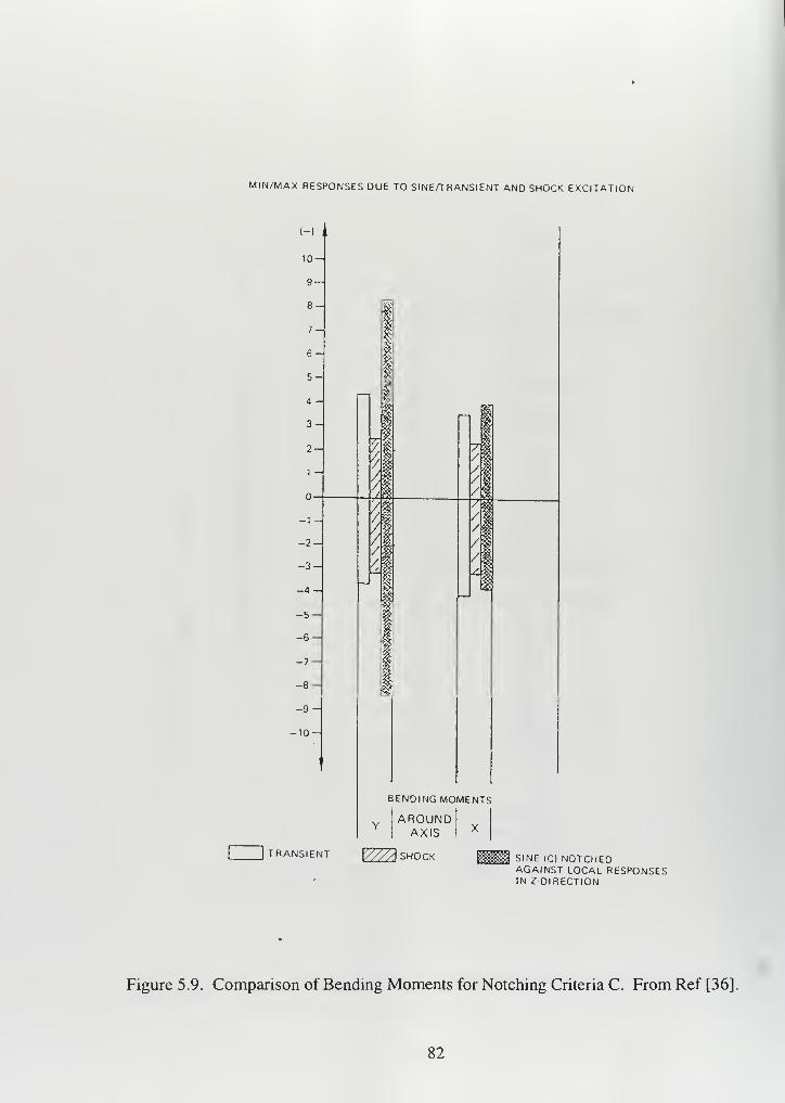
MIN/MAX RESPONSES DUE TO SINEATRANSIENT AND SHOCK EXCITATION
(-1II
10-
9
8
7-
6-
5-
4 -
3
2-
1-
-l H
-2
-3—
-4 -
-5-
-6-
-7 —
-8-
-9 -
-10—
BENDING MOMENTS
AROUNDAXIS
I ITRANSIENT V77A SHOCK SINE (C) NOTCHED
AGAINST LOCAL RESPONSESIN Z-DIRECTION
Figure 5.9. Comparison of Bending Moments for Notching Criteria C. From Ref [36].
82
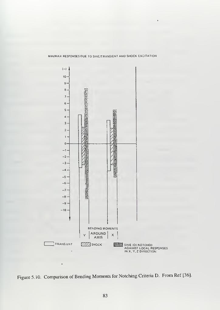
MIN/MAX RESPONSES DUE TO SINEAT RANSIENT AND SHOCK EXCITATION
(-) 4
10
9 —
8-
7-
6-
5
4 -
3
2-\
1
-1
-2
-3H
-4
-5 —
-6
-7 —
-8-
-9
-10-
BENDING MOMENTS
AROUNDAXIS
TRANSIENT ]///A SHOCK SINE (D) NOTCHEDAGAINST LOCAL RESPONSESIN X. Y. Z DIRECTION
Figure 5.10. Comparison of Bending Moments for Notching Criteria D. From Ref [36].
83

cm .
'
A I
:• ; i ji I i
I
ii ;*? !!:: : *i::il!:i i Htelii*
SPECIFIED INPUT IN 2 AT POINT 99
REALIZED INPUT IN 2 AT POINT 99
/.
_-
:
-
- -
-
1
___
H -
• -1
r
NOTCH CRITERIA :
LONGITUDINAL INTERFACE FORCE - 2850 NAT 40 to 46 Hz MEASURED DURING TRANSIENTTESTING
MEASUREDLONGITUDINALFORCE AT S/CINTERFACE
i'
r
"t'-'.T y?*~
T\z"
r
1
v1
','
i- . . .
—
-
NOTCH CRITERIA :
w.r.t LOCAL RESPONSES IN 2-DIRECTIONAT POINTS 2350/8553/10126
D -
;i;M. ;t Mil
.„___/:::::mmw ---
:::::]TIL if '
:
-+1~ J
' VILl I 1 "illi '
Figure 5.1 1. Notching Criteria. From Ref. [36].
84

(2) Swept Sinusoidal, Transient and Synthesized Waveform. As discussed
in References 20 and 37, laboratory testing was conducted at JPL to measure the relative
conservatism between vibration tests using several different inputs. These inputs included a flight-
transient excitation, swept sinusoidal and a synthesized waveform with the same SRS as the flight
waveform. Single axis tests were conducted on a dynamic mass model of a radioactive
thermoelectric generator (RTG) used in recent spacecraft. Several characterizations of the vibration
response of the structure were measured and compared. These characterizations included peak
acceleration levels and cycles, the rms acceleration as a function of time (TRMS), the rms
acceleration as a function of frequency (FRMS) and the shock response spectrum (SRS).
The input signals for these tests are shown in Figures 5.12 through 5.14. A
plot of the number of acceleration peaks exceeding a specific amplitude for each test input along
with flight data is shown in Figure 5.15. As expected, the swept sinusoidal input provides a much
greater number of peaks at a given amplitude than the flight data. In addition, the sinusoidal input
registers much higher maximum peak responses with significant numbers of peaks over 8 g's.
The transient test most closely follows the flight characterization, though the synthesized waveform
is close, resulting in only a small number of peak responses greater than the flight characterization.
Plots of the TRMS and FRMS characterizations for the transient and
synthesized waveforms are shown in Figures 5.16 and 5.17. As the duration of a test must be the
same to provide comparisons using these characterizations, data for the sinusoidal test was not
included. The TRMS plot indicates that the synthesized waveform results in moderate over testing
between 0.2 and 0.4 seconds while the transient input results in a slight under test throughout the
one second duration. The FRMS characterization, shown in Figure 5.17, shows that both the
transient and synthesized waveforms under test across the frequency range from 10 to 100 Hz.
Because the transient and synthesized waveforms can both be shaped to provide the response
desired, these variations from the desired response can be reduced.
85

3
21
1 3
<j
u
0.1 -
rt'
/
\ in,
\
i
li 1 ,
'
i
ill
1
Li.....
20 40 60
frequency (Hz)
Flight Test
100
Figure 5.12. Swept Sine Test and Flight Levels. From Ref. [37].
02 4 0.6 8 1
Tine (sees)
Figure 5.13. Transient Test and Flight Levels. From Ref. [37].
86

4 6
Time (sees)
Figure 5. 14. Synthesized Waveform Test and Flight Levels. From Ref. [37].
20,000 r
10,000
1,000
100
10
J i I > I ^_JL J I J_
2 4 6 8 10 12
Peak Ffesponse (G's)
F I igftt Transient SRS test Sine Steep
M
Figure 5.15. Number of Acceleration Peaks Versus Amplitude. From Ref. [37].
87

.4 0.6
Time (sees)
Fl i ght Trans ient SRS test
Figure 5.16. RMS Acceleration as a Function of Time. From Ref. [37].
1.5
r\
U 1
10
aIL
0.5
-
y^ i
_
X r...--
'_/'i , i i
20 40 60
Frequency (Kz)
Fl i ght Transient SRS test
100
Figure 5.17. RMS Acceleration as a Function of Frequency. From Ref. [37].
88

(3) Swept Sinusoidal, Random Dwell and Transient Comparison. This test
program, described in Reference 18, was initiated by Intelsat and conducted by Hughes to examine
alternatives to avoid the potential for over test inherent with notched swept sinusoidal testing. The
test objective was to subject the spacecraft to loads and responses representative of the flight
environment with respect to primary and secondary structure. At the time of the test, Intelsat
typically specified swept notched sinusoidal testing for the lower frequency range below 75 Hz,
which typically envelopes all primary and most secondary structural responses.
For this particular study, seven distinct tests were performed using a
prototype Intelsat IV-A vehicle:
1
.
baseline 4 oct/min notched swept sinusoidal input at 3/4 acceptance level.
2 . 8 oct/min notched swept sinusoidal input intended to reduce the number of cycles in
test.
3
.
4 oct/min notched swept sinusoidal with reduced control input and notch levels
identical to those used in the previous 4 oct/min test. The intent of this input was to
provide a narrower frequency region over which a resonance would notch,
reducing the number of load cycles and thus reducing the secondary response
4 . narrow band random dwell consisting of a 3 Hz bandwidth signal at three structural
resonances (7, 19, 23 Hz). For this test the input level was raised until the most
critical location reached the maximum expected flight response level.
5 . narrow band random dwell with broad band background floor. This test was
intended to excite secondary resonances at different frequencies from the primary
resonances.
6. direct transient reproduction at the spacecraft shelf. This test used a synthesized
base excitation which reproduced the transient response at the spacecraft shelf as
described in Chapter IV Section B.6.
7 . least favorable response at spacecraft shelf. This method attempts to establish a
transient base input which guarantees the maximum response at the spacecraft shelf.
89

As a basis for comparison, flight data was obtained for the Atlas Centaur as
discussed in Chapter IV, Section A.3. Cumulative amplitude histograms from a variety of
accelerometers provided information on the number of times the response exceeded a given level.
The histograms therefore provided information on the number of loading cycles as well as
magnitude. Comparative histograms for the flight and test data are shown in Figures 5.18 through
5.20.
Results of the 4 oct/min baseline sinusoidal sweep test, shown in Figure
5.18, show an excessive number of counts at high values of peak moment, which is clearly not
desirable. The reduced input 4 oct/min test results in a slight decrease in the number of
exceedances at a given level of peak moment but the 8 oct/min test shows the best correlation to
flight data in both number of cycles at high values of peak moment and general histogram
distribution.
tCK) J
rii«fc« Filth C InriitM T«« Cmih Hi)0)1 Una t Mt/alK
10)1 I1M I KIM.A Ml) II*. t KlhU, >-
^^U^>.10 30 «.C JO
1 of P»«h
Figure 5.18. Cumulative Amplitude Histogram for Sinusoidal Sweep Tests. From Ref. [18]
90

The random dwell histograms shown in Figure 5.19 indicate that the
random dwell input resulted in a response with a number of cycles in the low to mid peak moment
range that was greater than the flight results. However, this test did not produce the numbers of
high level load cycles shown in the flight environment. This could be remedied in the case of the
random test by just lengthening the duration of the test. This illustrates one of the benefits of the
random approach—the histogram can be shaped to produce the desired number of cycles at the
desired load level.
The results of the transient tests, as shown in Figure 5.20, show a
significant difference between flight and test. Because the synthesized transient used in this test
simulated the liftoff event only, the resulting histograms show fewer cycles at a given load level
than the flight histograms, which include all flight events. For an accurate test using the transient
method, all flight events must be simulated (such as MECO and BECO). While requiring
i 100
—~ ril|«l Mtc* Co— n inMUM T«r
O 10*1 l .«<«- tnll UIIMM lM«
° Jo*; *«•••- o~.ii vl tk rixi
Figure 5.19. Cumulative Amplitude Histogram for Random Dwell Tests. From Ref. [181
91

C 10 *0 100
Figure 5.20. Cumulative Amplitude Histogram for Transient Tests. From Ref. [18]
additional transient inputs, which would add to the duration of the required testing, this would not
be a significant complication.
As with the random dwell test, the transient tests offer the capability to
shape the histogram to more closely approach the flight composite. While the random test
histogram can be adjusted by either altering the duration of the test or adjusting the input levels, the
transient test histogram can be altered by varying the number of pulses at whatever load levels are
desired.
Comparative amplitudes for the various tests are shown in Table 5.8.
Results show that the sinusoidal sweep tests adequately tested the primary structure, with response
control of other primary structure channels limiting the adapter to only 89% of its peak limit
moment. However, the secondary structure was over tested up to 3850% even with peak limiting.
The 8 oct/min test reduced the cycle count while maintaining amplitude response of the primary
92
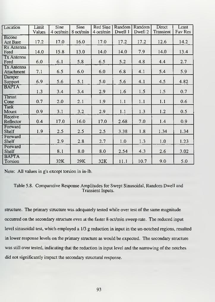
Location Limit
Values
Sine
4oct/minSine
8 oct/min
Red Sine
4 oct/min
RandomDwell 1
RandomDwell 2
Direct
Transient
Least
Fav Res
Bicone
Ant Base 17.2 17.0 16.0 17.0 17.2 17.2 12.6 14.2
Rx AntennaFeed 14.0 15.8 13.0 14.0 14.0 7.9 14.0 13.4
Tx AntennaFeed 6.0 6.1 5.8 6.5 5.2 4.8 4.4 2.7
Tx AntennaAttachment 7.1 6.5 6.0 6.0 6.8 4.1 5.4 5.9
DamperSupport 6.9 5.6 5.1 5.0 5.6 4.1 4.5 4.82
BAPTA1.3 3.4 3.4 2.9 1.6 1.5 1.5 0.7
Thrust
Cone 0.7 2.0 2.1 1.9 1.1 1.1 1.1 0.6
TankMount 0.9 3.1 3.2 2.9 1.1 1.3 1.2 0.5
Receive
Reflector 0.4 17.0 16.0 17.0 2.68 7.0 1.4 0.9
ForwardShelf 1.9 2.5 2.5 2.5 3.38 1.8 1.34 1.34
ForwardShelf 2.9 2.8 2.7 1.0 1.3 1.0 1.23
ForwardShelf 8.1 8.0 8.0 2.54 4.3 2.6 3.02
BAPTATorsion 32K 29K 32K 11.1 10.7 9.0 5.0
Note: All values in g's except torsion in in-lb.
Table 5.8. Comparative Response Amplitudes for Swept Sinusoidal, Random Dwell andTransient Inputs.
structure. The primary structure was adequately tested while over test of the same magnitude
occurred on the secondary structure even at the faster 8 oct/min sweep rate. The reduced input
level sinusoidal test, which employed a 1/3 g reduction in input in the un-notched regions, resulted
in lower response levels on the primary structure as would be expected. The secondary structure
was still over tested, indicating that the reduction in input level and the narrowing of the notches
did not significantly impact the secondary structural response.
93

The Table 5.8 data indicates that the random dwell input provided a very
good test for the primary structure. The secondary structure was still over tested by a significant
margin, in some cases worse than with the swept sinusoidal input. The random dwell input with
the floor addition was intended to boost the secondary response in non-resonant regions of the
primary structure. Data from the previous test shows, however, that the secondary response is
more than adequately excited by the lower input levels.
The transient test resulted in a slight under test of the primary structure.
However, the input pulse could be easily modified to increase the response as necessary, as long
as this did not result in over test to the secondary structure. In this case, the secondary structure
did experience an over test of up to 308% which is considerably less than the 3850% which
occurred with the swept sinusoidal input. The least favorable response test resulted in under
testing of the primary structure and most of the secondary structure.
(4) Swept Sinusoidal and Modulated Sinusoidal Pulse Comparison. As
discussed in Reference 22, loads predictions for the Galileo program showed significant low
(below 35 Hz) and mid (35-100 Hz) frequency transient vibration responses during launch events.
Because of concerns that slow swept sinusoidal testing would result in excessive resonance
buildup and an excessive number of vibration cycles, several alternative approaches were examined
by JPL for simulating the low frequency environment. These alternatives excitations included the
standard slow swept sinusoidal and a modulated sinusoidal pulse.
In preparation for testing of the Galileo Radioisotope Thermoelectric
Generator (RTG), a series of shaker vibration tests were conducted using a model represented by
the simplified one and two mass models shown in Figure 5.21. Test comparisons were made of
the slow swept sinusoidal and modulated sinusoidal pulse inputs. The modulated sinusoidal pulse
was generated as discussed in Chapter IV, Section B.6. The response at resonance and the
number of response cycles were determined for the two test cases along with a sinusoidal dwell
case for comparison. Because the Galileo load analysis indicated that spacecraft hardware
responses did not contain more than five high amplitude cycles for any significant launch vehicle
94

event, the modulated sinusoidal pulse used was limited to 5 cycles that exceeded 0.707 times the
maximum amplitude cycle.
^ V' M
2^ \
X
r
1 D.O.F. <System
k
tl
Ijjc.
\
2 D.O.F
I System
/
Figure 5.21. Model Used for Galileo RTG Tests. From Ref. [221
Analytical results for the response of a single degree of freedom system to sinusoidal
dwell, sinusoidal sweep and modulated sinusoidal pulse inputs are presented in Tables 5.9 and
5.10. The analytical data shows that the modulated sinusoidal input should result in an appreciably
lower response level than the sinusoidal sweep input while the number of cycles is clearly
excessive for the sinusoidal sweep input. While the actual test data was not published, according
to Reference 22, the analytical and test comparisons showed similar results.
Actual tests were conducted on the RTG and a Magnetometer Boom
Assembly using the modulated sinusoidal input. Pulses were space at one-third octave for the
RTG test and for the MBA pulses were specified at frequencies for all predicted transients of 2.7 g
peak or higher. Again, while actual results were not published, the transient tests were considered
successful and were recommended to replace the slow swept sinusoidal tests. However, recent
JPL programs
95

f TestI Response 0's pk |
1—-•__ M«WM— j ——
I SystemI Input |-—— - - -_—_——_—_—
|
Method | Condition1>m«C>ttt»E»M»»I»»tt
1 Q I G'splc:icxisxiii
|Fn «10 Hz|Fn«25 Hz|F n »50 Hz I
:cc:ciitiitiiittii:ticiizn
|
1 Sine | 10 seconds! 10 1.0 10 | 10
I 10 I
| ______________ ______ _________ ——— 1______ 1 ...
1
I Dwell | 30 seconds 10 1.0 10 I 10 1 10 1
I Sine | 2 oct/mln 10 1.0 9.7 1 9.5 1 9.1 1
1 Sweep| 6 oot/aln 10 1.0 9.5 1 9-3 1 9.0 1
1 Modulated | 5 cycles j
1 Sine | (2 0.707 1
I Pulses | max pulse |
1 | amplitude)|
10I 1.0
I 7.5 1 7.5 1 7.5
Table 5.9. Response of a SDOF System to Sinusoidal Dwell, Sinusoidal Sweepand Modulated Sine Pulse Inputs.
| Test | |Number of Cycles
I 1 1(2.0.707 • ntax response
I ! || Resonant Frequency
1 1 1 I 10 Hz | 25 Hz | 50 Hz
I Sine | 10 seconds | 10 I 100 I 250 I 500
| Dwell | 30 seconds I 10 1 300 1 750 1 1500
I Sine | 2 oct/mln I 10 I 43 I 108 I 216
| Swe«p | 6 oct/mlnI 10 I 14 I 36 I 72
IModulated I 5 cycles
I I I I
ISine
| (2 0.707 •I I I I
IPulses | max pulse
I 10 1 5 ! 5 1 5
I Iamplitude)
1 1 1 1
Table 5.10. Number of Response Cycles for a SDOF System with Sinusoidal Dwell,Sinusoidal Sweep and Modulated Sine Pulse Inputs.
96

such as Mars Observer and Cassini have not employed the modulated sinusoidal pulse technique.
In the case of Cassini, a force limited random vibration test has been adopted.
(5) Shock Spectrum Test Analysis. As discussed in references 8 and 38,
Intelsat dynamics tests through the advent of Intelsat V had consisted of 3-axis swept sinusoidal
testing and acoustic testing. With Intelsat V, shock spectrum testing was adopted to reduce the
risks of over testing during qualification for the Ariane Launch vehicle. The specification for the
test was in the form of a shock response spectrum as determined from the peak response of a
SDOF oscillator plotted vs. natural frequency. The shape of the SRS depends on the amplitude
and frequency content of the input waveform and the damping of the oscillator, as described in
Chapter IV, Section A.2. The drive waveform in this case was generated from a 1/6 octave
analysis of the synthesized SRS between 10 and 90 Hz. A Q of 10 was assumed in shaping the
input SRS.
Shock spectrum results for this test are presented in Table 5.11. While
there are no sinusoidal tests to compare to the shock spectrum tests, the response of the shock
spectrum test was in the range of the peak expected response. Initially, there was a significant over
test ranging from 1.5 to 2.0 times the predicted responses, most likely due to differences in the
impedance at the base of the satellite when bolted to a shaker table versus being attached to the
launch vehicle adapter. The SRS specification was then lowered to produce responses which
matched the predictions of the loads analysis. This lower specification was set at 72% of the
original SRS specification. Subsequent data from actual flight measurements on the FM-15
satellite adapter, which is located just above the bolted face to the Ariane adapter, shows that the
test SRS is very representative of the actual flight spectra. This flight spectra is shown in Figure
5.22. In this case, the peak excitation of the main axial mode was very near the upper limit for the
ground tests and the higher frequency components are all below the test specification limits. This
indicates that the shock spectrum method is a realistic simulation of the flight loads.
97

LOCATION PREDICTED RESPONSE(8)
MEASURED RESPONSE(g)
4 GHz Reflector 7-9 15
6 GHz Reflector 4.2 8
West Spot Reflector 4.3 11
Maritime Antenna 4.6 12
Momentum Wheel 2.4 4
Thruster Clusters 14.5-16 32
Propellant Tanks 7.2-9 9-10
Comm Transponder (N Side) 8 8
Comm Transponder (S Side) 8-9.5 9
Table 5.11. Intelsat V Shock Spectrum Response Data.
(6) Fast Swept Sinusoidal Test Analysis. The execution of the swept
sinusoidal test with a significantly increased sweep rate is discussed in references 7 and 39. This
approach is offered as an option when a higher cost digital controller is not available for
synthesized time waveform simulation of the transient environment. The intent is to reduce the
potential of over testing inherent with the slowly swept sinusoidal input by increasing the sweep
rate. The goal is to excite the test article at a higher sweep rate and adjust the input level to provide
the desired response. The sweep rate is determined by the number of cycles desired as determined
from flight acceleration time histories.
While an example of this approach was discussed, no experimental data was
provided to support the conclusions of the paper. This approach would clearly result in a reduction
of the number of cycles to which the test article is exposed. Based on the relationships presented
in Chapter IV, Section C.2 and as verified by the moderate increase in sweep rate discussed in
98

14
12 -en
co031
CDoo<
X<
10
4 "'
'!
Q-m" Fm-id/ v^d Maapier
Coupled AnalysisJ,
/\.1
*
yl V,?st SpLimits
ec.
-
/
\ \
- / . \ \
/
2^ 1 c
Jq^DCXX
—'
—
——.—
'
1
j—«—i—
—
f— —i -f
10 20 30 40 50 60 70 80 90 100
Frequency (Hz)
Figure 5.22. Flight Shock Response Spectrum from Intelsat VSatellite Adapter. From Ref. [8].
study number (3), this test method has some merit. However, with the current availability of
digital controllers, there has been little application of the fast swept sinusoidal method.
(7) Multi-Axis Vibration System Applications. Each of the previous
dynamics qualification studies and tests were based on the application of the vibration input in a
single axis. While testing may have been conducted in all three axis, independently, vibration
systems were typically not capable of excitation in multiple axes simultaneously. The relatively
recent development of multi-axis vibration systems (MAVIS) has enabled the excitation of any
rigid body motion in three axis with 6 degrees of freedom. MAVIS employment has taken place
almost exclusively in Europe, where multi-axis vibration test simulators previously used for
earthquake simulation have been employed to simulate launch vehicle multi-axis transients. The
multi-axis testing is considered to provide a more realistic simulation of the actual environment than
the classical single axis approach by providing correct super positioning of the multi-axial
structural loads.
99

Several studies of the potential application ofMAVIS to spacecraft
qualification testing have been performed. One such study, presented in Reference 40, discussed
the execution of transient testing in 6 degrees of freedom on a MAVIS table using a structural
model of the DFS-KOPERNIKUS telecommunications satellite. Test results comparing a transient
excitation of the DFS mass dummy at 50% amplitude with the desired specification levels are
shown in Figure 5.23. The plots show that the multi-axis system was able to very closely simulate
the environment in all 6 degrees of freedom. Slight deviations in the test results were due to
control system issues which required some modification to the control network.
While the feasibility of multi-axis transient testing has been shown, whether
such testing provides significant advantages to the qualification of a space vehicle is yet to be
proven. With the current focus on less expensive test methods, the cost of a multi-axis system
may not be justifiable to most spacecraft manufacturers.
100

I... — .M I t«H K..,.».,l .> |. ||
0.80.1
»
o.?
-0.6
-o e
o e
ObO.i
0./
-0.6
-0.6
-0.6
-o.e
6.0
».o
i.O
1.0
? .0
0.
-?
-u o
-6
6.0
1.0
?.o
^.0-^
-6
1 oo
.^A/wvv
—
I «c.--?) I <
I uoo
.0^1
: i-«oi
e
0.6
0.
«
0.?
-o i
-a v
-o 6
-o o
o.eo 6
I KD I uOO
(i) Specification (b) T«t
Figure 5.23. MAVIS Test Transient Response Data. From Ref. [40].
101

102

VI. CONCLUSIONS AND RECOMMENDATIONS
A. CONCLUSIONS
1 . Acceptance Testing
Test failure and on-orbit performance data available for this study indicate that acoustic
testing at the vehicle level provides an adequate workmanship and materials defect screen,
especially for mature programs. The data does not indicate that additional dynamics tests such as
sinusoidal or random vibration result in either an increase in the detection of failures during test or
a reduction in the early flight failure rate. Data from other test effectiveness studies supports this
conclusion. Additional data is required to generate a more thorough understanding of acceptance
test effectiveness as well as to provide statistical significance.
The experimental studies analyzed for this report provide no information on the
effectiveness of acoustic testing relative to sinusoidal and random vibration testing. However, the
JPL study clearly indicates that random vibration at appropriate levels is far more perceptive than
swept sinusoidal testing in exposing workmanship defects. As indicated by the Topaz II test data,
this result is demonstrated despite the fact that the random vibration test results in far lower
response levels throughout a typical space structure. Consequently, the random test at the vehicle
level provides greater test effectiveness with lower risk of damage to hardware. While there is no
experimental data to indicate how acoustic testing would rate, the failure data as discussed above
indicates that a similar acoustic experiment should result in ever greater failure detection rates.
2 . Qualification Testing
The studies and tests surveyed for the analysis of vehicle level qualification testing clearly
indicate that the single axis slow swept sinusoidal test provides an unrealistic simulation of the
flight environment. Even when notching is applied, the response levels especially for secondary
structure, can exceed actual flight values by significant margins. At the same time, other locations
can be significantly under tested. In addition, the slow swept sinusoidal test exposes hardware to
significantly greater numbers of cycles than the flight environment.
103

The studies surveyed almost uniformly indicate that a transient input developed either
directly from flight data or synthesized from the shock response spectrum very accurately simulates
the flight environment. The transient approach to dynamic qualification testing minimizes the risk
of over test while producing realistic responses with regard to magnitude and numbers of cycles.
With current digital control systems, such testing is relatively easy to conduct. Transient testing
clearly demonstrates significant utility when applied to spacecraft qualification testing and to the
validation of analytical models for complete design verification.
While offering simplicity in execution as well as a reduction in the potential for over
testing, there is not enough information to validate the effectiveness of the fast swept sinusoidal
approach for qualification testing. Similarly, MAVIS testing, while offering a more accurate
simulation of the launch environment, has not yet been developed to the point that significant
improvements in effectiveness can be shown.
B . RECOMMENDATIONS
The following recommendations are provided as a result of this study:
1
.
The Space Systems Engineering Database (SSED) developed by the Aerospace
Corporation under US Air Force sponsorship is a useful resource for the analysis
of spacecraft testing as well as a variety of other issues. The information currently
available in the SSED is an excellent start but should be supplemented with
additional data, especially from non-DOD programs which have traditionally
employed different test approaches. As the commercial spacecraft manufacturing
business is highly competitive, it is understandable that data from commercial
programs is not available. However, data from government programs should be
available and would greatly benefit the entire US space industry. In particular, it is
recommended that NASA and JPL data be added to the SSED as soon as possible.
2 . The utility of test data such as that in the SSED would be greatly enhanced if test
programs systematically documented failures with greater detail. Specifically, it is
104

recommended that data relating failures to the specific test in which they occurred
along with test levels and durations be recorded whenever possible for DOD and
other government sponsored test programs. Such data would greatly assist in the
analysis of test effectiveness. While the collection of this type of data would
increase costs in a test program, the long term benefits are significant.
3 . An acoustic workmanship study such as that conducted by JPL for sinusoidal and
random vibration inputs is recommended to further analyze the effectiveness of
acoustic tests for spacecraft acceptance.
4 . A more detailed study regarding fast swept sinusoidal testing for vehicle level
qualification tests is recommended to determine if such an approach would provide
an additional alternative to the slow swept sinusoidal test for spacecraft
qualification.
5 . With the continued development of multi-axis vibration systems, it is recommended
that additional data is collected to determine if the effectiveness of spacecraft
qualification testing is increased by the use of multi-axis techniques.
6 . The MIL-STD- 1540C focus on acoustic testing at the vehicle level appears to be
validated. However, the MIL-STD provides little discussion of the need for space
vehicle qualification in the low frequency quasi-static environment. As this
environment has been shown to be a significant design driver for both primary and
secondary structure, it is recommended that MIL-STD- 1540C incorporate more
detail with regard to qualification of the low frequency environment, either through
analysis or test.
105

106

APPENDIX A. TYPICAL LAUNCH ENVIRONMENT
SPECIFICATIONS
A. Delta 3000 Series Launch Vehicles.
Thrust Axis Lateral Axis
+2.8/ -1.4 3.4 for Payloads < 800 lb
2.9 tor P/L 800-1200 lb
2.4torP/L> 12001b
Table A. 1. Delta 3000 Series Liftoff Load Factors. From Ref. [14].
Vehicle
Configuration
Axial
(G)
Lateral
(G)
Payload
Wt. (lb)
3913 7.8 +/- 4.6 +/-1.0 > 1100
3920 7.0 +/- 4.1 +/-1.0 >4000
3914 7.5 +/- 4.6 4/- 1.0 >2000
3910 8.1 +/- 4.1 4/- 1.0 >2500
Table A.2. Delta 3000 Series Limit Load Factors at MECOat Spacecraft Center of Gravity. From Ref. [14].
Frequency
(Hz)
Shock Response Spectrum (G)
Qualification Acceptance
100
100-800
800-4000
15
+8.7dB/oct
200
11
+8.7 dB/oct
140
Table A. 3. Delta 3000 Series Shock Response Spectra, Q=10. From Ref. [14].
107

Frequency (Hz) ASD Level (G2/Hz)
20
20-300
300-700
700-2000
2000
.0016
+4dB/oct
.06
-3dB/oct
.021
Overall 87 Grms
Table A.4. Delta 3000 Series Spacecraft Random Vibration Limit Levels. From Ref. [14].
108

One-Third Octave
Center Frequency
(Hz)
Noise Level (dB) re: .00002 Pa
Qualification Acceptance
25-3240
122
123
125
119
.120
122
5063
80
126
127
127
123
124
124
100
125
160
130
132
134
127
129
131
200250315
134
135
137
131
132
134
400500630
137
142
137
134
139
134
800
10001250
134
132
130
131
129
127
160020002500
130
129
127
127
126
124
315040005000
127
125
125
124
122
122
6300800010000
123
121
121
120
118
118
Overall 147 144
Table A.5. Delta 3000 Series Acoustic Test Levels
(Inside Payload Fairing). From Ref. [14].
109

B Shuttle Transportation System (STS).
One Third Octave
Center Frequency (Hz)
Noise Level (dB) re: .00002 Pa
Protoflight Acceptance
25
3240
50
63
80
100
125
160
200
250315
400
500630
80010001250
160020002500
315040005000
6300800010000
122.0
125.0
128.0
130.5
131.5
132.0
132.0
132.0
131.5
130.5
130.0
129.0
128.0
127.0
126.0
124.5
123.0
121.5
119.5
118.5
116.0
114.5
112.5
111.0
109.0
107.5
106.0
119.0
122.0
125.0
127.5
128.5
129.0
129.0
129.0
128.5
127.5
127.0
126.0
125.0
124.0
123.0
121.5
120.0
118.5
116.5
115.5
113.0
111.5
109.5
108.0
106.0
104.5
103.0
Overall 142 139
Table A.6. STS Cargo Bay Acoustic Test Levels
(Up to 9 ft diameter payloads). From Ref. [14].
110
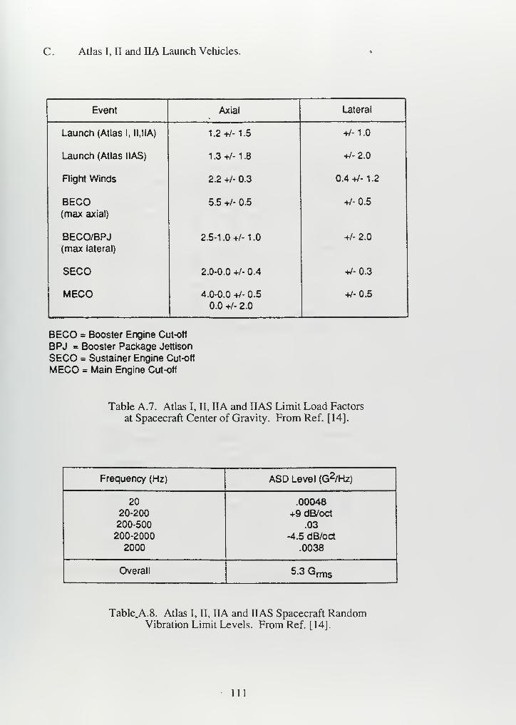
C . Atlas I, II and IIA Launch Vehicles.
Event Axial Lateral
Launch (Atlas 1, H.IIA) 1.2+/- 1.5 +/-1.0
Launch (Atlas MAS) 1.3+/- 1.8 +/-2.0
Flight Winds 2.2 +/- 0.3 0.4 +/- 1 .2
BECO 5.5 +/- 0.5 +/-0.5
(max axial)
BECO/BPJ 2.5-1 .0 +/- 1 .0 +/- 2.0
(max lateral)
SECO 2.0-0.0 +/- 0.4 +/-0.3
MECO 4.0-0.0 +/- 0.5
0.0 +/- 2.0
+/-0.5
BECO = Booster Engine Cut-oft
BPJ = Booster Package Jettison
SECO = Sustainer Engine Cut-off
MECO = Main Engine Cut-off
Table A.7. Atlas I, II, HA and IIAS Limit Load Factors
at Spacecraft Center of Gravity. From Ref. [14].
Frequency (Hz) ASD Level (G2/Hz)
2020-200
200-500
200-2000
2000
.00048
+9 dB/oct
.03
-4.5 dB/oct
.0038
Overall 5-3 Grms
Table.A.8. Atlas I, II, IIA and IIAS Spacecraft RandomVibration Limit Levels. From Ref. [14].
Ill

Frequency
(Hz)
Shock Response Spectrum (G)
Qualification Acceptance
100
100-1600
1600-4000
28
+10dB/oct
2800
20
+10dB/oct
2000
Table A.9. Atlas I, II, IIA and UAS Spacecraft Separation ShockResponse Spectrum, Q=10. From Ref. [14].
Frequency
(Hz)
Shock Response Spectrum (G)
Qualification Acceptance
100
100-500
500-4000
20+5.4 dB/oct
84
14
+5.4 dB/OCt
60
Table A. 10. Atlas I, II, IIA and HAS Payload Fairing and Insulation Jettison
Shock Response Spectrum, Q=10. From Ref. [14].
112

One-Third OctaveCenter Frequency
(Hz)
Noise Level (dB) re: .00002 Pa
Without Acoustic Blankets With Acoustic Blankets
Qualification Acceptance Qualification Acceptance
25
3240
121
123
124.5
118
120
121.5
121
123
124.5
118
120
121.5
50
63
80
126
128
129
123
125
126
126
128
129
123
125
126
100
125
160
130.5
132
132.5
127.5
129
129.5
130
131
131
127
128
128
200
250
315
133.5
134
133
130.5
131
130
131.5
131
129
128.5
128
126
400
500
630
132
131
129.5
129
128
126.5
127
125
123.5
124
122
120.5
8001000
1250
127
125
122
124
122
119
121
119
116
118
116
113
1600
20002500
120
119
118.5
117
116
115.5
114
113
112.5
111
110
109.5
315040005000
118
117.5
117
115
114.5
114
112
111.5
111
109
108.5
108
6300800010000
116.5
116
115.5
113.5
113
112.5
110.5
110
109.5
107.5
107
106.5
Overall 143 140 140 137
Table A. 1 1 . Atlas I, n, and HA Acoustic Test Levels (Inside 1 1 ft. Diameter
Payload Fairing). From Ref. [14].
113

114
LIST OF REFERENCES
MDL-STD-1540C, Test Requirementsfor Launch, Upper-Stage, and Space Vehicles, 15
September 1994.
Hamberg, O., Tosney, W., "The Effectiveness of Satellite Environmental Acceptance
Tests," The Journal ofEnvironmental Sciences, 1988.
Tosney, W., "Spacecraft Test Effectiveness Brief," The Aerospace Corporation, 1993.
"GOES Spacecraft Testing Process Brief," NASA Goddard Space Flight Center.
Harris, CM. and Crede, C.E., Shock and Vibration Handbook, McGraw-Hill, Inc.,
1976.
6. Moening, C.J., "An Overview of Shock, Vibration and Acoustic Environments," TheAerospace Corporation, 1988.
7 . Xian, H.Y., "A Simulated Method of Transient Environment—The Fast Swept Sine
Method," Proceedings of the Institute ofEnvironmental Sciences, 1981.
8. Lomas, N.S., Schrantz, P.R., "An Evaluation of Low Frequency Shock Spectrum Testing
For Intelsat V / Ariane Compatibility," International Symposium, Environmental Testing
For Space Programs, Test Facilities and Methods, 26-29, June 1990.
9. Hershfeld, D.J., "Avoiding Unrealistic Overtest By Notching the Vibration Test
Specification," Proceedings of the Institute ofEnvironmental Sciences, 191A.
10. Herzberg, R.J.,"Structural Dynamic Testing Considerations for Large Space Vehicles,"
Lockheed Missiles and Space Company, March 1974.
1 1
.
Ory, H., Hornung, E., "Real Launch Vehicle Flight Loads and Their Simulation ForSpacecraft Development," ERNO Raumfahrttechnik GmbH, Bremen, Germany.
12. Slone, R.M., "System Level Acoustic Testing," Proceedings of the Institute ofEnvironmental Sciences.
1 3
.
MIL-HDBK-340, Application Guidelinesfor MIL-STD-1540C; Test RequirementsforLaunch, Upper Stage, and Space Vehicles. June 1995.
1 4
.
GEVS-SE, General Environmental Verification Specificationfor STS and ELV Payloads,
Subsystems, and Components, NASA Goddard Space Flight Center, January 1990.
1 5
.
Coladonato, R.J., "Derivation of the Sinusoidal Sweep Vibration Test Levels for the
Cosmic Background Explorer," Proceedings of the I3tn Aerospace Testing Seminar, 1991.
1 6. "Atlas II DOD User's Mission Planning Guide," General Dynamics Space SystemsDivision, December 1988.
17. Voorhees, C, McKee, L., "Dynamic Testing of Spacecraft Structures," Sound andVibration , Vol. 24, Issue 1, January 1990.
115

18. Fowler, J.R., Zuziak, R.J., DesForges, D.T. and Schrantz, P.R., "Alternatives to
Notched Sine Testing for Spacecraft and Other Large Systems," Proceedings of theInstitute ofEnvironmental Sciences, April 1977.
19. Kern, D., Barrett, P., "Rationale for Cassini Spacecraft Random Vibration Test," Jet
Propulsion Laboratory Memorandum, 20 February 1996.
20. Hine, M.J., "Swept Sine Vibration Test Conservatism," Journal of the Institute ofEnvironmental Sciences, November-December 1995.
2 1
.
Agrawal, B.N., "Stability of an Automatic Notch Control System in Spacecraft Testing,"
Shock and Vibration Bulletin, January 1972.
22. Kern, D., "Vibration Problems-Transient Vibration Test Criteria," Jet Propulsion
Laboratory, California Institute of Technology, Pasadena, California.
23. Schlue, J., "Flight Payloads Environmental Approach," Proceedings of the Institute ofEnvironmental Sciences.
24. "Sine Vibration Testing Brief," Dynamics Environments Group, Jet Propulsion
Laboratory, June 1993.
25. Boatman, D., Scharton, T., Hershfeld, D. and Larkin, P., "Vibration and Acoustic Testing
of Topex/Poseidon," Journal of the 17th Space Simulation Conference, 9-12 November1992.
26. Milder, G., "Viking 1975 Orbiter DTM/Lander Dynamic Test Model DynamicEnvironmental Testing: An Overview," Proceedings of the Institute ofEnvironmental
Sciences, Vol 2, 14-16 April 1975.
27. Pike, H.S., Day, R., Gatta, J., "AUSSAT-B Spacecraft Qualification and Acceptance
Testing." Proceedings of the 13th Aerospace Testing Seminar, 8-10 October, 1991.
28. Ginsdorf, T., "Tailoring and Test Effectiveness," Jet Propulsion Laboratory, California
Institute of Technology, Pasadena, California.
29. Lang, P., Card, M.,"Application of Test Effectiveness in Spacecraft Testing,"
Proceedings of the Annual Reliability and Maintainability Symposium, 1995.
30. Ackerman, A. "Refining Test Effectiveness Through Systems And Cost-Of-Quality
Analysis, " Proceedings of the Institute ofEnvironmental Sciences.
3 1
.
Smith, D.A., "Evaluation of Spacecraft Acceptance Test Effectiveness," Proceedings ofthe Institute ofEnvironmental Sciences.
32. Smith, D.A., "System Level Acoustic Test Effectiveness," Proceedings of the Institute ofEnvironmental Sciences, 1986.
33. Hine, M.J., "Comparison of Workmanship Vibration Test Methods," Report D-12903, Jet
Propulsion Laboratory, 1995.
34. Raney, Elisa Anne, Vibration Analysis of Topaz II, Master's Thesis, Naval Postgraduate
School, June 1995.
116

35. Campbell, Sheryl Elaine, Random Vibration Analysis of the Topaz II Nuclear Reactor
Power System, Master's Thesis, Naval Postgraduate School, June 1995.
36. "Design Verification of Large Spacecraft." MBB Erno Report, Intelsat Contract No. Intel
276, MBB/ERNO Raumfahrttechnik GMBH, Bremen, Germany, July 1985.
37. Hine, M.J., "Evaluation of Conservatism in Low Frequency VibrationTest Control," Jet
Propulsion Laboratory, Pasadena, California.
38. Lomas, N. and Mullin, J., "Low-Frequency Shock Spectrum Testing of Intelsat VSpacecraft, " Proceedings of the Institute ofEnvironmental Sciences, March 1990.
39. Clevenson, S., Martin, D., Pearson, J., "Representation of Transient Sinusoids in the
Environmental Vibration Tests for Spacecraft," Proceedings of the Institute ofEnvironmental Sciences, 1965.
40. Muhlbauer, K., Schildt, U., Raasch, W. "Transient Vibration Testing of Spacecraft
Structures, Experience With Multi-Axial Base Motion and Combined Base Motion andPoint Force Excitation, " Proceedings of the International Conference on Structures andMechanical Testing, 19-21 October 1988.
41 . Melancon, P.S., "Fleet Satellite Communications Program." 1980.
117

118

BIBLIOGRAPHY
Ankrom, M. and Vicari, L., "Automated Process for Notched Sine Testing, " Proceedings of the
14tn Aerospace Testing Seminar, 1993.
Barrett, S., Maytum, B., "The Development of Sine Vibration Test Requirements For Viking
Lander Capsule Components," Proceedings of the Institute ofEnvironmental Sciences, 28 April-
1
May 1974.
Hoffman, A.R., "Galileo Environmental Test And Analysis Program Summary." Proceedings ofthe Institute ofEnvironmental Sciences, 8-10 October 1991.
Hoffman, A.R., Schlue, J.W., "Galileo Spacecraft System Level Environmental Test Results."
Proceedings of the 9th Aerospace Testing Seminar, 15-17 October 1985.
Kern, D., "Mars Observer Sine Vibration Testing Brief," Jet Propulsion Laboratory, California
Institute of Technology, 9 February 1988.
Lyon, R.H., Random Noise and Vibration In Space Vehicles, The Shock and Vibration
Information Center, United States Department of Defense, 1967.
O'Connell, M.R., "Effectiveness of Spacecraft Sine Vibration Testing Test Criteria," Report TETATO-0028. Jet Propulsion Laboratory, 1994.
Swales, T.G., Alexander, J. and Luzier, R., "ATS-F Notching Criteria as Determined by Analysis
and Test, " Proceedings of the Institute ofEnvironmental Sciences, 28 April - 1 May 1974.
119

120

INITIAL DISTRIBUTION LIST
1
.
Defense Technical Information Center 2
8725 John J, Kingman Road., Ste 0944Ft. Belvoir, VA 22060-6218
2
.
Dudley Knox Library 2
Naval Postgraduate School
411 Dyer Rd.Monterey, CA 93943-5101
3. Chairman 1
Department of Aeronautics and Astronautics, Code AA/CONaval Postgraduate School
Monterey, CA 93943-5 106
4 . Chairman 1
Space Systems Academic Group, Code EC/PZNaval Postgraduate School
Monterey, CA 93943-5101
5
.
Professor Brij N. Agrawal 2
Department of Aeronautics and Astronautics, Code AA/AGNaval Postgraduate School
Monterey, CA 93943-5 106
6 . Professor Barry S. Leonard 1
Department of Aeronautics and Astronautics, Code SP/LDNaval Postgraduate School
Monterey, CA 93943-5106
7. Professor Terry Alfriend 1
Department of Aeronautics and Astronautics, Code SP/ALNaval Postgraduate School
Monterey, CA 93943-5106
8. Mr. Tom Boyd 2
Naval Research Laboratory, Code 91 10-45
4555 Overlook Avenue, SWWashington, DC 20375
9. Mr. Bill Tosney 2
Environmental Criteria and Tests DepartmentThe Aerospace Corporation
P.O. Box 92957-M4/907Los Angeles, CA 90009-2957
10. CDR Alan D. Scott 2Air Test and Evaluation Squadron ONE (VX-1)NAS Patuxent River, MD 20670-5305
121


DUDLEY KNOX LIBRARY
NAVAL POSTGRADUATE SCHOOL
MONTEREY GA 93943-5101

DUDLEY KNOX LIBRARY
3 2768 00323877 5