naval postgraduate school · james n. fodor lieutenant, united states navy b.s., united states...

NAVAL POSTGRADUATE

SCHOOL

MONTEREY, CALIFORNIA

THESIS

Approved for public release; distribution is unlimited

DISTANCE LEARNING: THE IMPACT OF NOT BEING A RESIDENT STUDENT

by

James N. Fodor

March 2016

Thesis Advisor: Marigee Bacolod Co-Advisor: Latika Hartmann

THIS PAGE INTENTIONALLY LEFT BLANK

i

REPORT DOCUMENTATION PAGE Form Approved OMB No. 0704–0188

Public reporting burden for this collection of information is estimated to average 1 hour per response, including the time for reviewing instruction, searching existing data sources, gathering and maintaining the data needed, and completing and reviewing the collection of information. Send comments regarding this burden estimate or any other aspect of this collection of information, including suggestions for reducing this burden, to Washington headquarters Services, Directorate for Information Operations and Reports, 1215 Jefferson Davis Highway, Suite 1204, Arlington, VA 22202–4302, and to the Office of Management and Budget, Paperwork Reduction Project (0704–0188) Washington DC 20503.

1. AGENCY USE ONLY(Leave blank)

2. REPORT DATEMarch 2016

3. REPORT TYPE AND DATES COVEREDMaster’s thesis

4. TITLE AND SUBTITLEDISTANCE LEARNING: THE IMPACT OF NOT BEING A RESIDENT STUDENT

5. FUNDING NUMBERS

6. AUTHOR(S) James N. Fodor

7. PERFORMING ORGANIZATION NAME(S) AND ADDRESS(ES)Naval Postgraduate School Monterey, CA 93943–5000

8. PERFORMINGORGANIZATION REPORT NUMBER

9. SPONSORING /MONITORING AGENCY NAME(S) ANDADDRESS(ES)

N/A

10. SPONSORING /MONITORING AGENCY REPORT NUMBER

11. SUPPLEMENTARY NOTES The views expressed in this thesis are those of the author and do not reflect theofficial policy or position of the Department of Defense or the U.S. Government. IRB Protocol number ____N/A____.

12a. DISTRIBUTION / AVAILABILITY STATEMENT Approved for public release; distribution is unlimited

12b. DISTRIBUTION CODE

13. ABSTRACT (maximum 200 words)

The existing literature suggests there are no significant outcome differences between online and traditional degree programs in the civilian sector. Few studies have looked for such differences within military schools and colleges, specifically. Given the growing popularity of online and distance education degree programs, we study the impact of this particular mode of instructional delivery on the academic and subsequent job performance of military officer students enrolled at the Naval Postgraduate School (NPS). Using propensity score matching, we estimate the effects that being a distance learning (DL) student has on four performance outcomes: grade point average, graduation, promotion, and separation. We further subdivide the sample into various subgroups based on military service branch, warfare community, academic preparation, and school within NPS to determine the heterogeneous effects of DL within each subsample. The DL students studied performed significantly worse than equivalent resident students on every measurement. We found NPS students enrolled in DL degree programs obtain GPAs approximately half a letter grade lower, are less likely to graduate, are less likely to promote, and are more likely to separate from military service than their NPS resident student counterparts. Given these results, it is imperative to conduct additional research to ascertain what makes distance learning inferior to residency at the Naval Postgraduate School.

14. SUBJECT TERMSdistance learning, TQPR, graduation, promotion, separation

15. NUMBER OFPAGES

81

16. PRICE CODE

17. SECURITYCLASSIFICATION OF REPORT

Unclassified

18. SECURITYCLASSIFICATION OF THIS PAGE

Unclassified

19. SECURITYCLASSIFICATION OF ABSTRACT

Unclassified

20. LIMITATIONOF ABSTRACT

UU

NSN 7540–01–280–5500 Standard Form 298 (Rev. 2–89) Prescribed by ANSI Std. 239–18

ii


iii

Approved for public release; distribution is unlimited

DISTANCE LEARNING: THE IMPACT OF NOT BEING A RESIDENT STUDENT

James N. Fodor Lieutenant, United States Navy

B.S., United States Naval Academy, 2008

Submitted in partial fulfillment of the requirements for the degree of

MASTER OF SCIENCE IN MANAGEMENT

from the

NAVAL POSTGRADUATE SCHOOL March 2016

Approved by: Marigee Bacolod Thesis Advisor

Latika Hartmann Co-Advisor

William Hatch, Academic Associate School of Business and Public Policy

iv


v

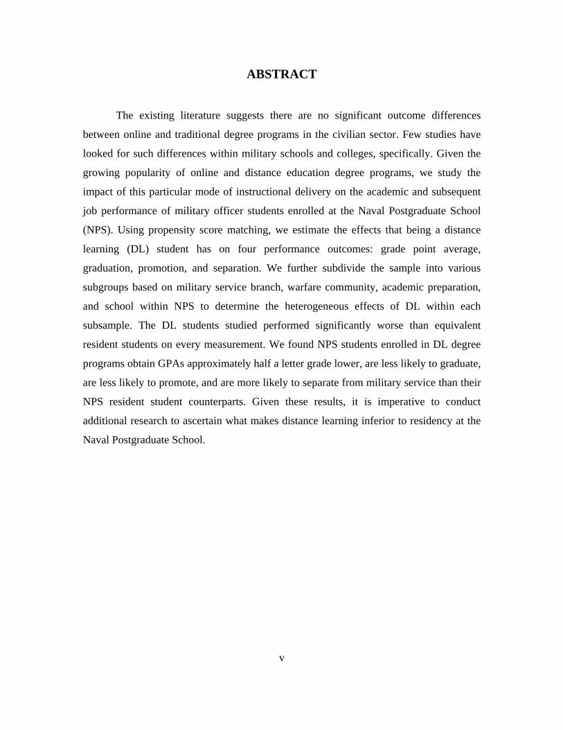
ABSTRACT

The existing literature suggests there are no significant outcome differences

between online and traditional degree programs in the civilian sector. Few studies have

looked for such differences within military schools and colleges, specifically. Given the

growing popularity of online and distance education degree programs, we study the

impact of this particular mode of instructional delivery on the academic and subsequent

job performance of military officer students enrolled at the Naval Postgraduate School

(NPS). Using propensity score matching, we estimate the effects that being a distance

learning (DL) student has on four performance outcomes: grade point average,

graduation, promotion, and separation. We further subdivide the sample into various

subgroups based on military service branch, warfare community, academic preparation,

and school within NPS to determine the heterogeneous effects of DL within each

subsample. The DL students studied performed significantly worse than equivalent

resident students on every measurement. We found NPS students enrolled in DL degree

programs obtain GPAs approximately half a letter grade lower, are less likely to graduate,

are less likely to promote, and are more likely to separate from military service than their

NPS resident student counterparts. Given these results, it is imperative to conduct

additional research to ascertain what makes distance learning inferior to residency at the

Naval Postgraduate School.

vi


vii

TABLE OF CONTENTS

I. INTRODUCTION..................................................................................................1 A. SCOPE OF THIS THESIS ........................................................................2 B. RESEARCH QUESTIONS .......................................................................2 C. ORGANIZATION OF THIS THESIS .....................................................3

II. LITERATURE REVIEW .....................................................................................5 A. META-ANALYSES ...................................................................................5 B. OBSERVATIONAL STUDIES ................................................................7 C. RANDOMIZED STUDIES .....................................................................10

III. DATA/METHODOLOGY ..................................................................................13 A. NPS DATA ................................................................................................13

1. Sample ...........................................................................................13 2. Independent Variables.................................................................13

a. Treatment Indicator ..........................................................13 b. NPS Institutional Controls ...............................................14 c. Academic Preparation.......................................................14 d. Service and Community ....................................................15

3. Dependent Variables ....................................................................16 B. DMDC DATA ...........................................................................................16

1. Sample ...........................................................................................16 2. Independent Variables.................................................................16 3. Dependent Variables ....................................................................16

C. IPEDS DATA ...........................................................................................17 1. Sample ...........................................................................................17 2. Variables .......................................................................................17

D. DATA SUMMARY ..................................................................................18 E. METHODOLOGY ..................................................................................26

1. Stage One ......................................................................................26 2. Stage Two ......................................................................................28

IV. RESULTS .............................................................................................................31 A. STAGE ONE ............................................................................................31 B. STAGE TWO ...........................................................................................32 C. HETEROGENEITY ................................................................................35

1. Service ...........................................................................................36 2. Community ...................................................................................36

viii

3. Rank ..............................................................................................37 4. APC ...............................................................................................38 5. Sector .............................................................................................38 6. School ............................................................................................39

V. SUMMARY AND CONCLUSIONS ..................................................................41 A. SUMMARY ..............................................................................................41 B. RECOMMENDATIONS .........................................................................41

APPENDIX A. PROPENSITY SCORE MATCHING–LOGIT RESULTS ..............43

APPENDIX B. OLS REGRESSION RESULTS FOR THE OUTCOME TQPR ......45

APPENDIX C. LPM REGRESSION RESULTS FOR THE OUTCOME GRADUATE .........................................................................................................47

APPENDIX D. LPM REGRESSION RESULTS FOR THE OUTCOME PROMOTED ........................................................................................................49

APPENDIX E. LPM REGRESSION RESULTS FOR THE OUTCOME SEPARATED .......................................................................................................51

APPENDIX F. OLS REGRESSION RESULTS FOR THE OUTCOME TQPR—HETEROGENEITY .............................................................................53

APPENDIX G. LPM REGRESSION RESULTS FOR THE OUTCOME GRADUATE—HETEROGENEITY .................................................................55

APPENDIX H. LPM REGRESSION RESULTS FOR THE OUTCOME PROMOTED—HETEROGENEITY ................................................................57

APPENDIX I. LPM REGRESSION RESULTS FOR THE OUTCOME SEPARATED—HETEROGENEITY ................................................................59

LIST OF REFERENCES ................................................................................................61

INITIAL DISTRIBUTION LIST ...................................................................................63

ix

LIST OF FIGURES

Figure 1. Military service branch comparison for DL and residency .......................20

Figure 2. Warfare community comparison for DL and residency ............................21

Figure 3. Military rank comparison for DL and residency ........................................21

Figure 4. NPS school comparison for DL and residency ..........................................22

Figure 5. APC 1 undergraduate GPA comparison for DL and residency .................22

Figure 6. APC 2 undergraduate mathematics background comparison for DL and residency .............................................................................................23

Figure 7. APC 3 undergraduate science and technical background comparison for DL and residency .................................................................................23

Figure 8. Undergraduate institution sector comparison for DL and residency .........24

Figure 9. Gender comparison for DL and residency .................................................24

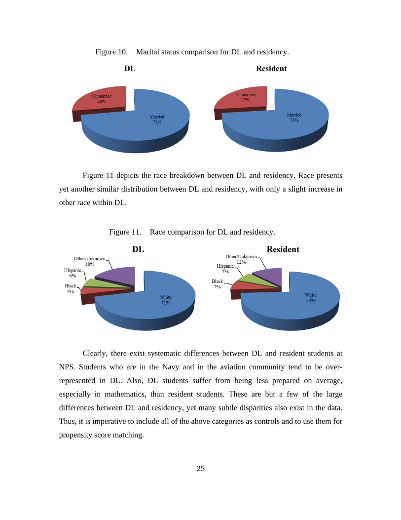
Figure 10. Marital status comparison for DL and residency. ......................................25

Figure 11. Race comparison for DL and residency. ....................................................25

Figure 12. Example propensity score matching overlay .............................................27

Figure 13. Propensity score matching overlay ............................................................32

x


xi

LIST OF TABLES

Table 1. Service and community breakdown ...........................................................15

Table 2. IPEDS sector breakdown ...........................................................................17

Table 3. Sample summary ........................................................................................19

Table 4. Independent variables ................................................................................27

Table 5. Average treatment effect summary ............................................................33

Table 6. Treatment heterogeneity by service ...........................................................36

Table 7. Treatment heterogeneity by community ....................................................37

Table 8. Treatment heterogeneity by rank ...............................................................37

Table 9. Treatment heterogeneity by APC ...............................................................38

Table 10. Treatment heterogeneity by sector .............................................................39

Table 11. Treatment heterogeneity by school ............................................................39

xii


xiii

LIST OF ACRONYMS AND ABBREVIATIONS

APC Academic Profile Code

DL distance learning

DMDC Defense Manpower Data Center

GSBPP Graduate School of Business and Public Policy

GSEAS Graduate School of Engineering and Applied Sciences

GSOIS Graduate School of Operational and Information Sciences

IPEDS Integrated Postsecondary Education Data System

LPM linear probability model

NCES National Center for Education Statistics

NPS Naval Postgraduate School

OLS Original Least Squares

SIGS School of International Graduate Studies

TUCE Test of Understanding College Economics

xiv


xv

ACKNOWLEDGMENTS

I would like to thank my wife, Amy. She has been nothing but patient,

understanding, and supportive throughout this entire process. Without the calm and

loving environment, or the occasional redirection—“You’d better get off that couch and

get back to writing”—she provided, it’s likely I’d never have finished.

I would also like to thank my two advisors, Dr. Marigee Bacolod and Dr. Latika

Hartmann. I cannot even imagine how much worse this process and resulting thesis

would have been without their guidance, help, and patience.

xvi


1

I. INTRODUCTION

The last decade has seen a growing interest in determining the impact of distance

or online forms of education on grades and subsequent job performance. Given the lower

cost of delivering such degrees, the motivation to move to online based programs has

increased substantially in recent years. While these cost savings are certainly relevant in

the civilian context, the military recognizes the potential for additional cost savings by

not having to relocate personnel for the sole purpose of higher education.

This popularity and cost savings have led to much academic research on the

subject. Overall, the findings on the impact of distance or online educational class

formats on academic performance show little to no significant difference between online

and traditional programs. Although, existing studies do indicate that synchronous

distance education formats are inferior to asynchronous formats and that effects tend to

be heterogeneous with weaker students performing proportionally worse in distance

formats. However, the current research focuses heavily on civilian institutions. This

prompts the question: Is the impact of distance education on academic and job

performance outcomes similar at military institutions, such as the Naval Postgraduate

School (NPS)?

NPS offers several online degree programs that come under the broad umbrella of

distance learning (DL) programs. The Graduate School of Operational and Information

Sciences (GSOIS) offers six DL master’s programs in computer science related

curriculums. The Graduate School of Engineering and Applied Sciences (GSEAS) offers

eleven DL master’s programs in engineering related curriculums. The Graduate School of

Business and Public Policy (GSBPP) offers four DL master’s programs in business and

contract management related curriculums (Naval Postgraduate School, 2016).

In this thesis, I estimate the impact of DL on student performance and subsequent

labor market outcomes for NPS military students. To achieve this end, I merge data from

three sources—the Institutional Research, Reporting, and Analysis Office at NPS, the

Defense Manpower Data Center (DMDC), and the Integrated Postsecondary Education

2

Data System (IPEDS)—to create a large sample of students with extensive information

on their demographics, undergraduate institution, and military career progression. Using

propensity score matching, I estimate the impact of DL on four performance outcomes:

grade point average, graduation, promotion, and separation. I further subdivide the

sample into various subgroups based on military service branch, warfare community,

academic preparation, and school within NPS to determine the heterogeneous effects of

DL within each subsample.

My findings indicate that DL students at NPS on average have lower grades, are

less likely to graduate, are less likely to promote in their subsequent military career, and

are more likely to separate from active service. Similar to the literature from the civilian

sector, I also find heterogeneous effects of DL. However, at NPS lower-ability DL

students do not perform worse compared to higher-ability DL students.

A. SCOPE OF THIS THESIS

This thesis analyzes NPS students in both DL and resident programs with

academic year start dates between 2006 and 2013. Data for the years in question and

provided by the Institutional Research, Reporting, and Analysis Office at NPS is merged

with data from the Defense Manpower Data Center (DMDC) and the Integrated

Postsecondary Education Data System (IPEDS) to supplement the range of students with

additional demographic, undergraduate institution, and promotion information. The

analysis addresses whether or not there is a difference between DL and resident student

performance and career progression.

This research is quantitative in nature. I conduct a review and evaluation of

relevant literature with a focus on distance education and online programs and their

perceived impact on university systems. I also use other literature to provide information

relevant to my research topic.

B. RESEARCH QUESTIONS

1. What is the causal impact of distance learning on military officer students’ academic and job performance?

3

2. What student characteristics best predict success in distance learning vs. resident learning?

3. Are there systematic differences between distance learning and resident military officer demographic characteristics, MOS, ability, and/or academic preparation?

C. ORGANIZATION OF THIS THESIS

This thesis consists of five chapters. Chapter I provides a brief introduction to the

subject matter and methodology. Chapter II presents a review of relevant literature with a

focus on the impact of distance education on performance outcomes. Chapter III

delineates the data utilized for analysis, demonstrates difference between DL and resident

student bodies, and provides an in depth insight into the methodology behind this thesis.

Chapter IV presents and explains the findings of this thesis. Finally, Chapter V provides

concluding remarks and preliminary recommendations.

4


5

II. LITERATURE REVIEW

Given the recent growth in distance education degree programs within the U.S.

military and beyond, there is an increasing need to better understand the impact of

distance education on student learning outcomes. Hence, the large literature on the topic

continues to grow more extensive with each passing year. The current literature falls into

three categories: meta-analyses, observational studies, and randomized experiments. I

summarize the main findings from these categories in order below.

A. META-ANALYSES

Meta-analyses are a quantitative summary of existing studies and present a

general picture of the state of research in a particular subject area. I focus on three key

and recent studies here that focus on how online and distance education modes of

delivery impact outcomes. A U.S. Department of Education meta-analysis conducted by

Means, Toyama, Murphy, Bakia, and Jones (2010) looks explicitly at online education

versus traditional face-to-face instruction focusing on post-secondary education. Lack

(2013) expounds upon Means et al. (2010) and provides additional insight for future

studies in this area. Unlike these studies, Bernard et al. (2004) focus explicitly on

distance education, separate from online education, and discuss at length the issue of

synchronous versus asynchronous delivery methods. Additionally, there are a variety of

outcomes used throughout the many smaller studies included in these meta-analyses,

including individual course grades, overall grade point average, instructor evaluation

surveys, and student evaluation surveys. However, the best and most common outcome

chosen is individual student course grade because it allows for a degree of control

between different classes and instructors and bypasses the more qualitative nature of

surveys.

Means et al. (2010) initially set out to provide information for K-12 students.

However, the vast majority of existing studies revolve around secondary and post-

secondary education, excluding any significant measures of effect for the intended

student body (2010, p. 31). Also, they drop a large number of studies that simply

6

compare online and traditional students, as they are likely to be biased by a student’s

selection into a particular type of course. By screening and eliminating all but 45 from a

pool of 1,132 existing studies, Means et al. do provide several significant results relevant

to continued education (2010, p. 14). After combining studies and weighting results

based on respective sample sizes, they find that the online delivery method is just as

effective as face-to-face instruction but not any better (Means et al., 2010, p. 18). Also,

the evidence suggests that supplementing classroom instruction with online resources,

often known as hybrid delivery, has a positive and significant impact on student

performance as measured by grades (p. 19). Further, the types of delivery media among

online courses demonstrate no significant effect on average learning outcomes (Means et

al., 2010, p. 40). Means et al. (2010) also highlight the wide variation in methods,

findings, and effect sizes across studies. The wide variation in methodologies likely

contributes to the wide variation in findings. Also, although they eliminated studies based

on the level of qualitative analysis and chosen outcome variables and then weighted

based on sample size, many studies were severely biased and lacking in good quality

control variables (Means et al., 2010, p. 13).

Lack (2013) conducts a meta-analysis similar to that of Means et al. (2010) but

with several key differences with regard to her focus. Lack (2013) identifies 30 studies

that compare some combination of face-to-face, online, and/or hybrid learning. She also

only includes studies with learning outcomes, such a course grades, as dependent

variables and precludes studies with student authors (p. 8). Instead of attempting to

calculate overall effects, Lack (2013) asserts that the existing literature is inadequate to

determine whether or not online or hybrid learning modalities are more or less effective

than traditional face-to-face modalities (p. 10). The discussion, in turn, revolves around

the shortage of quality studies, small sample sizes, and need for random assignment

(Lack, 2013, p. 8). In particular, this study highlights four general problems with the

current state of research. First, those studies that achieve random assignment to distance

education have very small sample sizes. Second, those studies with large samples often

lack sound experimental design and display widely conflicting results. Third, existing

observational studies generally fail to account for self-selection bias despite controlling

7

for background information. And finally, the remaining studies comprise those that

neglect relevant controls (Lack, 2013, p. 11–12).

Bernard et al. (2004) conduct yet another meta-analysis, although older than the

previous two. This study focuses exclusively on distance education, which can be

separate from online education that does not involve geographic separation. Findings

include a small yet significant positive effect of distance education on learning outcomes

(Bernard et al., 2004, p. 404). However, the standard errors are large, and thus the overall

result tends to be more in accordance with Means et al. (2010) of no significant

differences in student outcomes across delivery modes. What causes this study to stand

out is the emphasis on the effects of synchronous and asynchronous methods of distance

education. Synchronous distance education results in a significant negative effect on

learning outcomes, while asynchronous distance education results in a significant positive

effect on learning outcomes (Bernard et al., 2004, p. 404). Further, all three outcomes

measured—achievement, attitude, and retention—yield conflicting results between

synchronous and asynchronous formats. With respect to all three outcomes, synchronous

formats favor the classroom environment, whereas asynchronous formats favor distance

education (Bernard et al., 2004, p. 408).

These large meta-analyses draw on a vast body of observational studies and a

smaller body of randomized studies. I discuss each of these in turn next. Randomized

experiments account for selection bias, but are often limited in other areas due to

difficulty in designing and implementing proper experiments within university systems.

Observational studies face difficulty correcting for selection bias or simply do not even

attempt to account for it.

B. OBSERVATIONAL STUDIES

Koch (2006) conducted an interesting observational study at Old Dominion

University. He utilized data from 1994 to 2001 on all courses with both a distance

learning and resident component (p. 24). He utilizes the resulting sample of 20,428

observations to perform OLS regressions of student characteristics on individual course

grades (Koch, 2006, p. 25). Koch’s (2006) findings indicate that distance learning has a

8

very small impact, if any, but demographic characteristics do significantly impact student

grades (p.26–28). The incredibly large sample size and diverse set of control variables

represent this study’s greatest strengths. However, these strengths may not be enough to

balance the potential biases on account of students who selected into the residence and

distance learning courses. That said, the study highlights the need to include key

demographic variables when analyzing the impact of distance education.

Brown and Liedholm (2002) perform another observational study, but take a more

focused approach than Koch (2006). They attempt to compare face-to-face classroom,

hybrid, and virtual—their term for completely online class—versions of a Principles of

Microeconomics class. All three versions of the class were designed to be very similar

and utilize similar resources. The virtual version also gained access to recorded lectures

from the face-to-face class with an additional synchronous text based component (Brown

& Liedholm, 2002, p. 444). Brown and Liedholm (2002) find that students in the virtual

version of class consistently score approximately half a letter grade below students in the

face-to-face and hybrid classes (p. 447). Interestingly enough, they designed the study

and acquired demographic data as a control, but they made no attempt to correct for

selection bias or control for subtle, yet controllable, difference between class versions.

For example, different instructors taught the face-to-face and hybrid classes (Brown &

Liedholm, 2002, p. 444). Another issue exists in the small and disproportionate sample

size. With only 363 face-to-face, 258 hybrid, and 89 virtual student observations, the

study lacks substantial power (Brown & Liedholm, 2002, p. 445).

Gratton-Lavoie and Stanley (2009) conduct a study with a slightly different

methodology. They observe eight sections of an introductory economics class over four

semesters to compare online and hybrid delivery methods (p. 7). Using summary

statistics of final exam scores, Gratton-Lavoie and Stanley (2009) conclude that online

education has a positive effect on learning outcomes (p. 12). However, this method is

problematic because it neglects to consider potential impacts other than delivery mode on

exam score. They next use a probit model to estimate the likelihood of selecting online

over hybrid. From these likelihood values, they further assert that self-selection bias

shifts the positive effect found earlier to an insignificant or negative one, which they do

9

not quantify (Gratton-Lavoie & Stanley, 2009, p. 20). Despite their attempt to control for

selection, their small sample of 149 students lacks sufficient power to estimate the effects

of online and hybrid delivery (p. 12). Also, as mentioned above, utilizing summary

statistics to compare average final exam scores between online and hybrid courses

presents serious limitations as a basis for determining the overall effect of online

education on learning outcomes. They should utilize regression analysis when

determining effect size to control for additional factors that may impact learning

outcomes, such as previous academic performance or demographic information.

Coates, Humphreys, Kane, and Vachris (2004) perform another observational

study but with a heavy focus on correcting for any self-selection. They obtain data from

three separate universities for introductory microeconomics and macroeconomics courses

(Coates et al., 2004, p. 535). Coates et al. (2004) utilize three separate models—OLS,

2SLS, and an endogenous switching equation—in an attempt to ascertain the influence of

selection bias on Test of Understanding College Economics (TUCE) scores between

online and face-to-face students. They find that selection bias presents a substantial effect

and that the direction of the bias points toward zero (Coates et al., 2004, p. 545). The

presence of effect estimates biased toward zero when ignoring selection sheds additional

light on the multitude of observational studies with findings of “no significant difference”

between online and face-to-face modalities (Coates et al. 2004, p. 545). Also of note,

Coates et al. (2004) present one of the few studies to address systematic differences

between students self-selecting online courses rather than face-to-face offerings. They

find that students selecting online or distance options are overwhelmingly employed full

or part time in addition to school, have 300 point lower SAT scores on average, and tend

to perform better at online courses compared to students selecting face-to-face courses

(Coates et al., 2004, p. 545). Despite the lack of any real tangible effect, this study fills a

crucial gap in the literature by addressing the importance of handling selection bias when

comparing student performance between online and face-to-face courses. However, as

with many studies on the topic, Coates et al. (2004) have only a very small sample.

Samples for the various models used range from only 59 to 126 observations (p. 537–

544).

10

Olitsky and Cosgrove (2012) perform a unique observational study attempting to

account for self-selection bias. They compare multiple sections of Principles of

Microeconomics and Principles of Macroeconomics courses, designing courses with a

great deal of control between blended and face-to-face versions (Olitsky & Cosgrove,

2012, p. 19). Utilizing exam scores as outcome variables, they also find no significant

difference in effects between blended and face-to-face versions (Olitsky & Cosgrove,

2012, p. 30). This study stands out for its method of correcting for self-selection bias.

Olitsky and Cosgrove (2012) determine the average treatment effect of blended learning

by utilizing propensity score matching to create a matched sample, mitigating the

potential for selection bias (p. 27). It is this same method that we employ in our study to

correct for selection bias. As such, Olitsky and Cosgrove (2012) provide a clear

precedent for the use of propensity score matching to correct for self-selection bias when

unable to randomly assign students between treatment and control groups.

However, despite such methods of correction for selection bias among

observational experiments, random assignment of students provides the only true means

of completely eliminating such bias. Consequently, the following randomized

experiments represent some of the best attempts to determine the effect of distance

education within the current field of study.

C. RANDOMIZED STUDIES

Harmon, Alpert, and Lambrinos (2014) design an experiment to emulate random

assignment of students. They randomly divide a Principles of Economics class into

various portions of online or face-to-face delivery based on chapters. They then compute

the likelihood of answering midterm and final exam questions correctly based on whether

the associated questions correspond to online or face-to-face portions of the course using

a logit model (Harmon et al., 2014, p. 116–118). Harmon et al. (2014) reiterate the “no

significant difference” (p. 118) findings of several other studies, yet their approach

remains unique. However, this uniqueness coupled with a very small sample of 36

students leads to several issues. The article lacks clarity on many details and leaves the

reader unsure as to the validity of the approach. For example, Harmon et al. (2014) make

11

no mention of the number of sections, and based on sample size a single section is likely.

This implies that particular exam questions were only either observed as online or face-

to-face when computing estimates. The resulting lack of control among outcome

variables suggests the potential for serious bias. Harmon et al. (2014) may eliminate self-

selection bias from their sample, but shortcomings elsewhere leave much to be desired.

Bowen, Chingos, Lack, and Nygren (2014) design a randomized experiment

spanning six different universities. They compare traditional and hybrid formats for a

statistics course and conclude that hybrid formats offer a “no-harm-done” alternative that

also results in less time—both for instruction and completion of deliverables—for

students (Bowen et al., 2014, p. 107). This otherwise well designed experiment does

suffer from a lack of control among instructors, which is openly presented to the reader

(Bowen et al., 2014, p. 101). Also, this study uses the largest sample among randomized

experiments with 605 participants (Bowen et al., 2014, p. 98).

Perhaps the most widely cited study within the field, Figlio, Rush, and Yin (2010)

conduct a randomized experiment comparing exam scores between online and live

versions of a Principles of Microeconomics course (p. 766). Figlio et al. (2010) offer

students extra credit points in exchange for participating in an experiment. They then

randomly assign the 327 students agreeing to participate to either live or online versions

of the class (Figlio et al., 2010, p. 767). Figlio et al. (2010) find no statistical difference in

outcomes between online and live versions of the class (p. 779). Also of note, the nature

of the experiment makes comparison to distance learning difficult. For example, students

in the online section still had access to instructor office hours and could schedule

individual face-to-face meetings with the instructor (Figlio et al., 2010, p. 766).

Joyce, Crockett, Jaeger, Altindag, and O’Connell (2014) conduct another

randomized experiment comparing traditional and hybrid formats. They also offer extra

credit points in exchange for participation. They observe the 656 participants spread

through eight sections of a Principles of Microeconomics course, and outcome variables

include midterm and final exams, Applia coursework, course final grades, and

withdrawals (Joyce et al., 2014, p. 6–9). Joyce et al. (2014) find that “traditional does

moderately better” (p. 27), and on average students in traditional versions perform

12

2.5 percentage points higher on exams than those in hybrid formats (p. 28). Despite the

seemingly common small sample size, this study performs exceptionally well. Joyce et al.

(2014) manage to control for a multitude of factors such as minimizing differences

between classes and resources and including a large set of demographic and academic

performance variables.

Alpert, Couch, and Harmon (2015) perform one of the best randomized studies so

far. They randomly assign participants, who again were offered extra credit for

participation, into either face-to-face, online, or hybrid sections of a microeconomics

principles class between Fall of 2012 and Spring of 2014 (Alpert et al., 2015, p. 3–4).

Alpert et al. (2015) utilize three stages of OLS regressions—each stage increasing the

number of controls—to determine the effects of the three class formats on cumulative

final exams scores (p. 4). They find that blended format never yields a significant effect,

but online classes result in a significant and consistent decrease of approximately half a

letter grade (Alpert et al., 2015, p. 27). The only concern with this study again comes in

the form of a relatively small sample size, but this seems to be a pervasive issue among

randomized experiments.

The existing literature presents several relevant methodologies as well as many

concerns. No studies exist addressing the issue of online or distance education compared

to resident education for military officer students. In designing my study I attempt to

apply the lessons presented above to a sample of military officer students at NPS.

Unfortunately, I am unable to achieve the gold standard of conducting a randomized

experiment. However, I instead focus on a methodology derived from both Koch (2006)

and Olitsky and Cosgrove (2012). Because Koch (2006) found a large impact of

demographics on performance outcomes, I focus on a large sample with robust

demographic controls. Also, I utilize propensity score matching, similar to Olitsky and

Cosgrove (2012), to mitigate biases resulting from students self-selecting into either

distance or resident delivery modes.

13

III. DATA/METHODOLOGY

Utilizing several of the strengths spread across studies within the existing

literature, I design an observational study to estimate the impact of DL on learning and

military performance outcomes. I merge data from three separate sources—the Naval

Postgraduate School (NPS), the Defense Manpower Data Center (DMDC), and the

Integrated Postsecondary Education Data System (IPEDS)—to create a sample

containing the necessary demographic controls. I then use propensity score matching to

correct for bias resulting from selection into either DL or residency programs. Finally, I

conduct regression analysis to determine the impact of DL on various academic and

military performance related dependent variables. This section addresses each of these

data sources and methodologies in turn.

A. NPS DATA

1. Sample

The primary data come from a Python extract provided by the Institutional

Research, Reporting, and Analysis Office at NPS. These data were used in a master’s

thesis by Kyle Alcock at NPS in March 2015, but that study focused only on a sample of

Naval officers. The subjects in my study initially consist of the population of 10,882 NPS

students—U.S. military officers, civilians, and international students—who began

academic programs between the 2006 and 2013 academic years. Civilian and

international students are excluded from the analysis sample, as I cannot match DMDC

information to them. After dropping all civilian and international students the sample size

decreases to 6,754 observations.

2. Independent Variables

a. Treatment Indicator

The NPS data provide the binary variable for DL, where DL equals one for

students enrolled in NPS DL degree programs. DL is the indicator of treatment for this

study.

14

b. NPS Institutional Controls

I generate cohort control variables from academic start year and quarter

information. Also, school indicators allow control for the four different schools at NPS:

the Graduate Schools of Business and Public Policy (GSBPP), the Graduate School of

Engineering and Applied Sciences (GSEAS), the Graduate School of Operational and

Information Sciences (GSOIS), and the School of International Graduate Studies (SIGS).

c. Academic Preparation

NPS utilizes academic profile codes (APC) as the primary means for determining

academic eligibility and student academic preparation prior to admission at NPS. A

student’s APC consists of three discrete digits, each representing a different aspect of his

or her academic background. The first digit represents undergraduate academic

performance based on GPA, the second digit represents mathematics background and/or

elapsed time since college level math course completion, and the third digit represents

engineering, science, or technical background (Naval Postgraduate School, 2016). To

control for student preparation I generate dummy variables for each digit of APC

indicating whether each student has met the requisite APC for his or her particular

curriculum.

Also, the NPS data include information on both undergraduate school name and

time elapsed from completion of an undergraduate degree prior to beginning studies at

NPS. Undergraduate school name allows for the merger with IPEDS data from the

National Center of Education Statistics (NCES) that indicate the sector—private vs.

public and for-profit vs. not-for-profit—of the college of university the military officer

graduated from. In addition, I use undergraduate school name to generate an indicator of

whether the student attended a service academy. With a completely military sample,

attending a service academy also represents a level of academic preparation. Finally,

because there is variation in elapsed time between undergraduate and graduate educations

among NPS DL and resident students, the inclusion of the continuous variables for years

since undergraduate education seems relevant as yet another measure of academic

preparation.

15

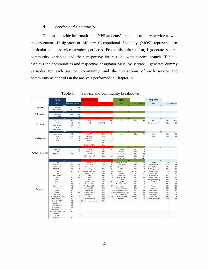
d. Service and Community

The data provide information on NPS students’ branch of military service as well

as designator. Designator or Military Occupational Specialty (MOS) represents the

particular job a service member performs. From this information, I generate several

community variables and their respective interactions with service branch. Table 1

displays the communities and respective designator/MOS by service. I generate dummy

variables for each service, community, and the interactions of each service and

community as controls in the analysis performed in Chapter IV.

Table 1. Service and community breakdown

Job Designator Approx. n Job MOS Approx. n Job MOS Approx. n Job MOS Approx. n

Surface 1110 786

Surf. Undes. 1160 28

Submarine 1120 302

Sub. Undes. 1170 45

General 1300 10 Pilot 75xx 146 Aviation 15xx 47 Pilot 11xx 126

Pilot 1310 729 NFO 7525/7528 33 Combat Sys. Off. 12xx 36

Pilot Undes. 1390 21

NFO 1320 279

NFO Undes. 1370 3

Oceanography 1800 93 MAGTF 02xx 29 Intel 35xx 71 Intel 14xx 72

IWO 1810 83 Ground 02xx 7 Cyber 17xx 16

IPO 1820 66 CI/HUMINT 02xx 4

Intel 1830 75 SI/EWO 02xx 12

Air 02xx 14

CI/HUMINT OPS 02xx 3

Spec. War 1130 46 Infantry 03xx 51 Infantry 11xx 100

EOD 1140 29 Tank Off. 18xx 4 Armor 19xx 2

EOD Undes. 1190 1 AAV Off. 18xx 2 Field Artillery 13xx 87

Field Artillery Off. 08xx 38 A/D Artillery 14xx 17

Special Forces 18xx 247

EDO 1440 11 Adjutant 01xx 39 Imm. & Personnel 00xx 29 Weather 15xx 71

EDO Undes. 1460 281 Logistics Off. 04xx 81 Corps. of Eng. 12xx 68 Ops. Support 16xx 42

AEDO Aero 1510 44 Comms. Off. 06xx 111 Signal Corps. 25xx 52 Security Forces 31xx 19

AEDO Maint 1520 78 Combat Eng. Off. 13xx 25 MP 31xx 7 Civil Engineering 32xx 16

PAO 1600 174 Ground Supp. Off. 30xx 66 Psy. Ops. 37/39xx 5 Public Affairs 35xx 10

FAO 1710 13 Finance Off. 34xx 32 Civil Affairs 38xx 27 Personnel 38xx 12

FAO Undes. 1720 42 PAO 43xx 3 Space Ops. 40xx 1 Biomedical Sp 43xx 2

HR 1200 189 JAG 44zz 6 Adjutant Gen. 42xx 10 Scientific Research 61xx 11

Medical 2100 10 MP 58xx 5 Finance 44x 7 Developmental Eng. 62xx 44

Dental 2200 3 A/C Maint. Off. 60xx 22 Foreign Affairs 48xx 8 Acquisitions 63xx 61

Medical Service 2300 65 Avioincs Off. 63xx 1 Acquisitions Off. 51xx 8 Contracting 64xx 79

Flight Surgeon 2302 1 Avn. Supply Off. 66xx 27 Medical 60xx 1 Finance 65xx 24

JAG 2500 7 Air C&C Off. 72xx 9 Medical Service 67xx 9 Special Inv. 71xx 53

Nurse 2900 12 Low Alt. A/D 72xx 9 Transportation/Logistics 88xx 14 A/C Maint. 21xx 17

Supply 3100 332 Air Supp. Control 72xx 11 Ammunition/Maint/Ord. 91xx 20 Missile Maint. 21xx 2

Chaplain 4100 2 A/D Control 72xx 8 Quartermaster 92xx 16 Readiness 21xx 24

Civil Engineering Corps 5100 20 ATC 72xx 10 O.R./Sys Analysis 49/57xx 4 Spec. Duty 88xx 2

Spec. War LDO 6152 1 Avn. Acquisitions 80xx 1 Chemical 74xx 8 Students/candidates 92xx 13

Elec. Surf. LDO 6180 1 Defense Systems Analyst 88xx 1

Eng. Sub LDO 6232 1

Elec. Sub LDO 6280 1

Comm. Sub LDO 6290 1

Avn. Maint. LDO 6330 6

Air Traffic Control LDO 6390 1

Admin LDO 6410 5

IS LDO 6420 2

Met/Ocean LDO 6460 1

467 294 502

Ground Combat

Support

1304

453

317 69 71 88

076 95

Surface

Submarine

Aviation

1042 179

0

0 0 0

Intelligence

47 162

347

814 0 0

Navy Marine Corps. Army Air Force

16

3. Dependent Variables

The NPS data provide three of the five dependent variables that I analyze. Total

quality point rating (TQPR) is essentially a GPA calculated for all courses taken at NPS

(Naval Postgraduate School, 2015). I use TQPR as the primary and only continuous

outcome variable. It would be advantageous to utilize individual course grades instead of

overall TQPR, but this information is currently unavailable for the existing sample. I also

include binary outcome of whether a student graduates.

B. DMDC DATA

1. Sample

As Koch (2006) makes clear, sound demographic control variables are necessary

when ascertaining the impact of DL. DMDC data provide these important demographic

controls for the sample, as well as subsequent career progression of these students upon

leaving NPS. Demographic data were requested for the entire sample as of six months

prior to beginning their studies at NPS, while work performance data was requested

covering the period after leaving NPS. Thus, the sample size remains the same, and forty-

seven additional observables are added.

2. Independent Variables

Of the additional observable characteristics added, I focus on key demographic

variables including: gender, race, marital status, age, number of dependents, and rank.

Race consists of variables for white, black, Hispanic, and other race. Marital status

includes two dummy variables, one indicating whether an observation was married

during his or her time at NPS and the other indicates if the observations had ever

experienced a divorce. Rank indicates the military paygrade of an observation upon

beginning enrollment at NPS. The fourteen resulting variables cover the range of

demographics typically controlled for.

3. Dependent Variables

DMDC data provide the remaining two outcome variables in this study, which are

promotion and separation status. The dependent variable “promoted” indicates students

17

who received a promotion after departure from NPS, whether or not they had actually

received a degree. Separated indicates those officers that separated from military service

for any reason after leaving NPS.

C. IPEDS DATA

1. Sample

IPEDS is a branch of the National Center for Education Statistics (NCES) and

provides downloadable and publically available data for accredited schools offering

postsecondary education within the United States (National Center for Education

Statistics, 2016a). I merge the 2012 IPEDS database, which is the most applicable, to the

existing sample based on undergraduate degree institution listed in the NPS data.

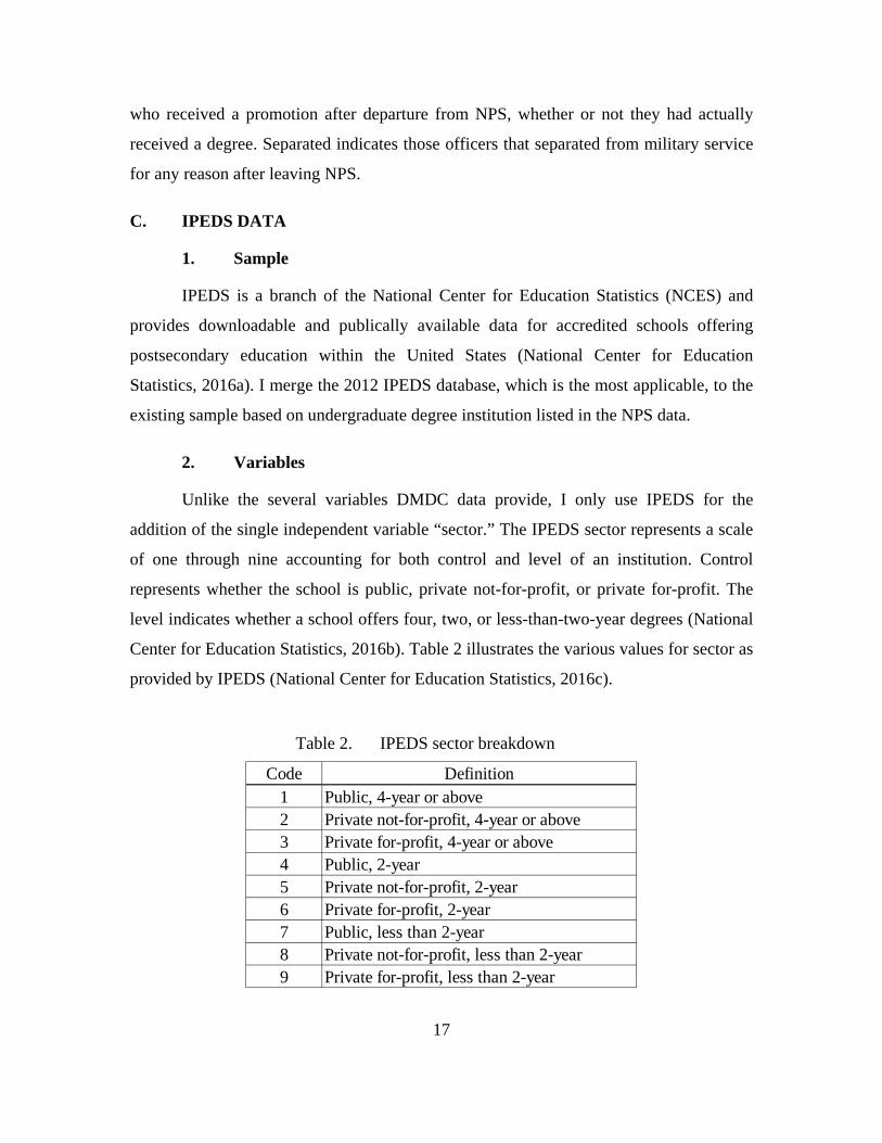
2. Variables

Unlike the several variables DMDC data provide, I only use IPEDS for the

addition of the single independent variable “sector.” The IPEDS sector represents a scale

of one through nine accounting for both control and level of an institution. Control

represents whether the school is public, private not-for-profit, or private for-profit. The

level indicates whether a school offers four, two, or less-than-two-year degrees (National

Center for Education Statistics, 2016b). Table 2 illustrates the various values for sector as

provided by IPEDS (National Center for Education Statistics, 2016c).

Table 2. IPEDS sector breakdown

Code Definition1 Public, 4-year or above2 Private not-for-profit, 4-year or above3 Private for-profit, 4-year or above4 Public, 2-year5 Private not-for-profit, 2-year6 Private for-profit, 2-year7 Public, less than 2-year8 Private not-for-profit, less than 2-year9 Private for-profit, less than 2-year

18

However, I focus solely on the control classification because commissioned

officers overwhelmingly possess four year degrees. As such, I generate three control

variables for the entire sample: public, private not-for-profit, and private for-profit.

Additionally, I define these three variables so that they are exclusive of Service Academy

graduates. Service Academies fall under public category according to IPEDS, however

based on selectivity and average student performance prior to postsecondary education

they are more akin to private not-for-profit institutions. For this reason, and because a

large proportion of NPS students are Service Academy graduates, I utilize the variable

“Service Academy” from the NPS data to represent a fourth component of sector.

D. DATA SUMMARY

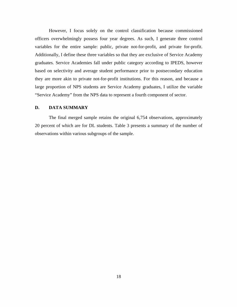
The final merged sample retains the original 6,754 observations, approximately

20 percent of which are for DL students. Table 3 presents a summary of the number of

observations within various subgroups of the sample.

19

Table 3. Sample summary

DL Resident All1,331 5,423 6,754

Navy 1,182 2,773 3,955Marine 54 767 821Army 16 910 926Air Force 69 887 956Surface 104 710 814Submarine 122 225 347Aviation 697 764 1,461Intelligence 24 690 714Ground Combat 33 776 809Support 337 2,449 2,786O1 29 122 151O2 46 473 519O3 706 2,883 3,589O4 272 1,726 1,998O5 130 50 180O6 14 4 18Public 457 2,461 2,918Private not-for-profit 223 1,108 1,331Private for-profit 5 41 50Service Academy 412 1,230 1,642GSBPP 772 1,150 1,922GSEAS 361 1,055 1,416GSOIS 190 1,697 1,887SIGS 8 1,384 1,392Met APC 1 1,019 4,863 5,882Met APC 2 845 4,166 5,011Met APC 3 1,084 4,887 5,971Female 70 523 593White 949 4,021 4,970Black 64 356 420Hispanic 82 375 457Other Race 236 671 907Married 961 3,963 4,924Divorced 4 102 106

APC

Dem

ogra

phic

sSe

rvic

eC

omm

unity

Ran

kSe

ctor

Scho

ol

Full SampleBy Variable:

20

There are several systematic differences between DL and resident students.

Figures 1 through 11 illustrate the differences between DL and resident students based on

the independent variable categories of service, community, rank, school, APC,

undergraduate degree institution sector, gender, marital status, and race.

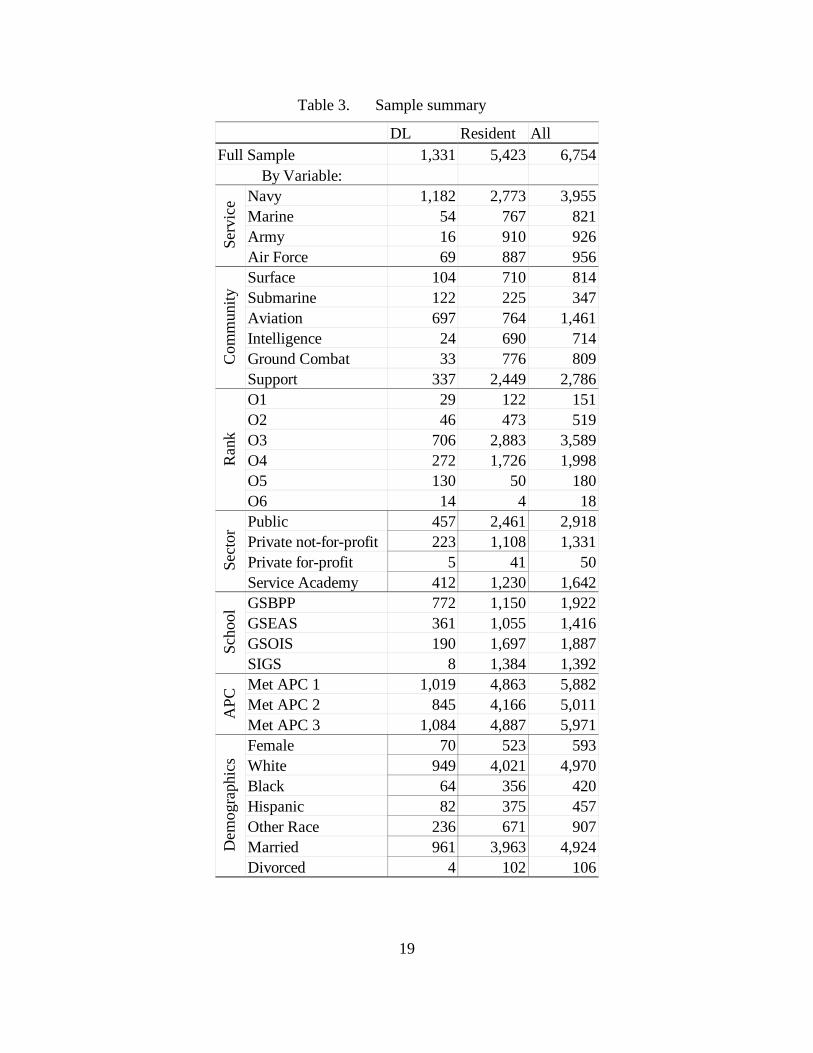
A comparison of services between DL and residency are depicted in Figure 1.

Unsurprisingly, Navy students comprise the majority among residents. However, for DL

this majority nearly doubles. Marine Corps, Army, and Air Force students comprise only

about 10 percent of all DL students at NPS between 2006 and 2013.

Figure 1. Military service branch comparison for DL and residency

Warfare communities are depicted in Figure 2. The makeup of DL and resident

students is quite different. In particular, aviators tend to favor and/or get assigned to DL

programs more than other communities. While aviators only make up approximately 12

percent of all resident students between 2006 and 2013, they comprise more than half of

the DL students for the same period. The disparities presented only reinforce the need to

control for both service and community in assessing student outcomes, and also in order

to make an apples-to-apples comparison.

21

Figure 2. Warfare community comparison for DL and residency

Figure 3 illustrates rank breakdowns between DL and residency. The only

substantial differences seem to be a decrease in O-2’s, a decrease in O-4’s, and an

increase in O-5’s within DL. Figure 4 shows the increased representation of GSBPP

within DL compared to residency, while also displaying a decreasing representation by

GSOIS and SIGS.

Figure 3. Military rank comparison for DL and residency

22

Figure 4. NPS school comparison for DL and residency

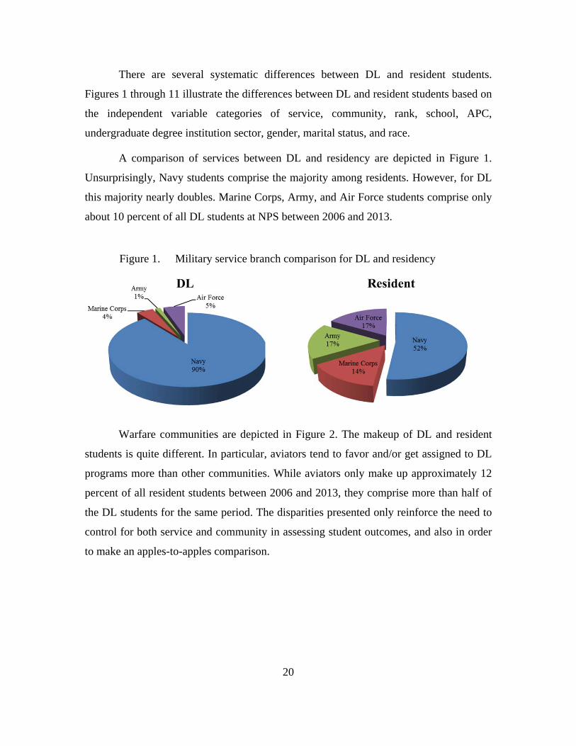
Figures 5 through 7 depict whether or not students met the required APCs for

their respective curriculums. Interestingly enough, comparing APC results show that DL

students tend to be far less prepared with regard to all APC’s than resident students. The

greatest gap is in APC 2 (mathematics background).

Figure 5. APC 1 undergraduate GPA comparison for DL and residency

23

Figure 6. APC 2 undergraduate mathematics background comparison for DL and residency

Figure 7. APC 3 undergraduate science and technical background comparison for DL and residency

Figure 8 depicts the IPEDS sector breakdown. Sector distribution in DL is

comparable with the distribution in residency programs, with no difference in overall

percentage of private not-for-profit and private for-profit institutions. However, students

with undergraduate degrees from public institutions decrease by 10 percentage points

within DL compared to residency, while an increase in Service Academy graduates

makes up the difference. Gender, shown in Figure 9, also shows only a small difference

between DL and residency. There are 4 percentage points fewer females in DL than in

residency.

24

Figure 8. Undergraduate institution sector comparison for DL and residency

Figure 9. Gender comparison for DL and residency

DL and resident military students tend to be similarly distributed with regard to

marital status as well. Figure 10 shows that DL students represent only 1 percentage point

more unmarried students than their resident counterparts.

25

Figure 10. Marital status comparison for DL and residency.

Figure 11 depicts the race breakdown between DL and residency. Race presents

yet another similar distribution between DL and residency, with only a slight increase in

other race within DL.

Figure 11. Race comparison for DL and residency.

Clearly, there exist systematic differences between DL and resident students at

NPS. Students who are in the Navy and in the aviation community tend to be over-

represented in DL. Also, DL students suffer from being less prepared on average,

especially in mathematics, than resident students. These are but a few of the large

differences between DL and residency, yet many subtle disparities also exist in the data.

Thus, it is imperative to include all of the above categories as controls and to use them for

propensity score matching.

26

E. METHODOLOGY

The method of propensity score matching conceptually involves creating

counterfactual outcomes of what would have happened to DL students had they gone

through a resident program, and what would have happened to resident students had they

been through a DL program.

The matching methodology is broken down into two distinct stages. Stage One

involves creating a matched subsample from the existing sample. Stage Two of my

analysis then uses the matched sample to conduct regression analysis and determine the

impact of DL on performance outcomes. I further discuss the methodology behind these

two stages in the next two sections.

1. Stage One

Propensity score matching is a statistical technique that allows for the creation of

a matched sample where observations are similar enough between treatment and control

groups to efficiently and unbiasedly determine the average effect of the treatment. Also,

on can determine the treatment effect on the treated using this method. Matching relies on

the key assumption that subjects that are similar based upon observable characteristics are

likely also similar on unobservable characteristics (Gertler, 2011). In this study, the

variable DL represents treatment. Consequently, within a matched sample, those

observations enrolled in DL are similar with respect to observable characteristics, and

thus also unobservable characteristics, to those enrolled as resident students. In a sense,

this process is simulating a nonexistent control group as a counterfactual for the purposes

of examining the effect of DL on learning and job performance outcomes. Thus, the

counterfactual match to a DL student is identified by finding a control resident with the

same propensity to be in DL and vice versa.

To create this matched sample, I start by determining the probability that each

observation is enrolled in DL. Considering DL is a binary variable, a Logit model suits

this purpose well. Equation 1 specifies this logit model, where the associated independent

variables are defined in Table 4.

27

0 1 2 3 4

0 1 2 3 4(DL 1)

1

i i i i

i i i i

b b DEMO b ACAD b MIL b CHRT

i b b DEMO b ACAD b MIL b CHRT

eprob

e

(1)

Table 4. Independent variables

Upon estimating this regression, predicted values of DL are calculated for all

observations. I then utilized a kernel density function to plot probability density overlays

for both DL=1 and DL=0. This overlay allows for visual inspection of the region of

common support, or the region where observations are similar in their propensity for

treatment (Gertler, 2011). Ideally the probability distributions do not overlap perfectly, as

the goal is to eliminate dissimilar observations at the far left and right ends of the overlay.

Figure 12 presents an example overlay plot.

Figure 12. Example propensity score matching overlay

Source: Gertler, 2011, p. 110

Demographic Controls (DEMO) Academic Controls (ACAD) Military Controls (MIL) Cohort Controls (CHRT)Female Years since Undergraduate Degree (Continuous) Service (Navy Reference) School (GSBPP Referece)Race (White Reference) Sector (Public Reference) Community (Support Reference) Cohort Year (2006 Reference)Married Met APC 1, 2, 3 Service Community Interactions Cohort Quarter (Q1 Reference)Divorced Rank (O-3 Reference)Age (Continuous)Number of Dependents (Continuous)

28

To achieve a sound probability overlay requires some trial and error. I modified

the model in Equation 1 several times to acquire a desirable overlay and satisfy the

necessary assumption of common support. I eventually acquire a suitable region of

common support by attempting various combinations of independent variables. I then

create the final matched sample by eliminating observations that fall outside the region of

common support.

2. Stage Two

Stage Two is simply conducting a normal regression analysis using the matched

sample. To form unbiased and efficient estimates, I use the inverse of propensity scores

generated from the first stage as weights in the second stage regressions. Four outcome

variables are evaluated to ascertain the impact of DL. TQPR is the only continuous

outcome, while Graduated, Promoted, and Separated are all binary dependent variables.

An original least squares (OLS) regression is an obvious choice for TQPR, however the

binary dependent variables require some thought.

I initially specify the three binary outcomes as logit models. Upon closer

examination, I realize that a Linear Probability Model (LPM) is the superior choice. The

logit model derivatives, or marginal effects, for all binary outcomes are nearly identical

to the coefficients of a similarly specified LPM. Further, the LPM’s key weakness lies it

its ability to produce predicted values less than zero or greater than one, which are not

feasible probability values (Woolridge, 2013). I generate predicted values for a LPM

regression of each binary outcome and summarize the results. For each outcome, the

predicted values fall within the acceptable range between the 5th and 95th percentiles.

Also similar to its OLS counterpart, the LPM is the best linear unbiased estimator. Thus,

the LPM is both qualitatively and quantitatively the superior choice of model. Equations

2 and 3 depict the specifications for continuous and binary outcomes, respectively.

0 1 2 3 4 5i i i i i iy b b DL b DEMO b ACAD b MIL b CHRT (2)

0 1 2 3 4 5( 1)i i i i i iprob y b b DL b DEMO b ACAD b MIL b CHRT (3)

29

Due to the matching process, b1 represents the treatment effect of DL in both

Equations 2 and 3. Under propensity score matching assumptions, this treatment effect is

also free of self-selection bias.

The final step involves running several regressions to determine the heterogeneity

of DL’s effect within different subgroups of the matched sample. I run a series of 112

separate regressions where each service, community, rank, APC, sector, and school are

isolated. Equations 4 and 5 depict the specifications for continuous and binary outcomes,

respectively, where CONTROLj indicates the subgroup being examined in isolation.

0 1 ,s. t .CONTROL 1i i jy b b DEMO (4)

0 1( 1) ,s. t .CONTROL 1i iprob y b b DEMO j (5)

These final models allow comparison of DL’s effect between different services,

communities, ranks, schools, and among those students that did or did not meet the

requisite APC for their curriculum.

30


31

IV. RESULTS

In this chapter, I present the results in three sections. First, I show the first stage

results of the matching exercise. Second, I present the second stage results estimating the

impact of DL on the four outcome variables, namely TQPR, Graduate, Promoted, and

Separated. Finally, I test for heterogeneous effects of DL within subgroups of the

matched sample.

A. STAGE ONE

As mentioned in Chapter III, to create a matched sample I first regress observable

characteristics of students on an indicator for DL participation using logistic regressions.

The key observable factors included in the logit model are demographic characteristics,

military service branch, warfare community and its associated interactions with service

branch, and military rank. The full results of this regression appear in Appendix A. It is

important to note that gender, marital status, time elapsed since undergraduate education,

undergraduate university sector, service branch, the support community, and support

community and service interactions are all significant predictors of enrolling in DL. Also,

the ranks of O-2 and O-3 are significant predictors of selection of DL programs as well.

From the logistic regression, I calculate predicted values for the likelihood of DL

enrollment and then plot probability density overlays for different combinations of

observable characteristics. Figure 13 shows the probability density functions separately

for resident and distance learning students.

32

Figure 13. Propensity score matching overlay

The x-axis of the plot in Figure 13 represents the propensity score. These values

represent the predicted values resulting from the logistic regression. The region of

common support exists between approximately 0.1 and 0.3. Observed students falling

outside of this range are eliminated from the sample as they are significantly dissimilar to

those within the region of common support. Doing so results in a matched sample of

5,289 observations. This reduction of only 1,465 students from the initial sample results

in a matched sample that is sufficiently large and robust to provide statistical power to

my analysis.

B. STAGE TWO

Table 5 displays the average treatment effect (ATE) of DL for each performance

outcome. These results are representative of the entire matched sample. Also, full

regression results appear in Appendices B through E.

01

23

45

De

nsity

0 .2 .4 .6 .8 1Pr(dl)

Residence Learning Distance Learning

33

Table 5. Average treatment effect summary

The first row of Table 5 focuses on the results for TQPR (average GPA). All else

equal, the TQPR of students in DL programs is 0.3998 points below resident students.

This result is statistically significant at the 1 percent level. This negative impact translates

into almost half a letter grade reduction in a DL student’s TQPR compared to an

equivalent resident student.

It is also important to note that DL is not the only factor that affects TQPR.

Appendix B displays complete regression results for this outcome. Married students on

average have higher TQPRs than unmarried students. Marine Corps students have

approximately a half a letter grade higher TQPR than Navy students. Surface warfare

officers and submariners both have lower TQPRs than support officers, while Naval

Aviators have higher TQPRs. Students in GSEAS, GSOIS, and SIGS all have lower

TQPRs than students in GSBPP. Finally, service academy graduates have significantly

higher TQPRs than students that graduated from public institutions for their

undergraduate degree. Interestingly, meeting APC 3 results in a 0.2127 point reduction in

TQPR on average.

Based on the existing literature, it appears that NPS students enrolled in DL

programs are significantly worse off than their civilian equivalents. These results are

somewhat inconsistent with the common overall findings of little to no significant

difference between traditional and online class formats. However, they are consistent

with the findings of Bernard et al. (2004) in that synchronous distance programs perform

0.0562*** [0.0203]

ATE of DLOutcome

Robust standard errors in brackets*** p<0.01, ** p<0.05, * p<0.1

TQPR

Graduate

Promoted

Separated

-0.3998*** [0.0735]

[0.0272]-0.2232***

-0.1253*** [0.0276]

34

worse than asynchronous equivalents. The NPS DL programs being synchronous support

the general finding of lower performance in the synchronous format compared to

asynchronous.

The second row of Table 5 shows the results for graduation. All else being equal,

I find that DL results in a decrease in the probability of graduating by 22.32 percentage

points on average. This negative impact is significant at the 1 percent level. This result

implies that even if resident programs achieved a 100 percent graduation rate, that DL

equivalents would suffer more than one-fifth of their students failing to complete

programs of study. Again, synchronous DL at NPS seems more detrimental than existing

literature would suggest.

Similar to TQPR, other factors significantly affect the chances of graduating from

NPS. For example, Appendix C shows that on average black students are 11 percentage

points less likely to graduate than white students. Also like TQPR, being a surface

warfare officer or a submariner results in a negative impact on the probability of

graduation. Marine Corps support officers and Air Force support officers are also less

likely to graduate. Further, O-5s are less likely to graduate than O-3s and students in

SIGS are not significantly less likely to graduate than GSBPP students. Again, meeting

APC 3 has a negative impact on the probability of graduation. However, APC 2 shows a

7 percentage point increase in the probability of graduating.

The third row of Table 5 suggests DL students are less likely to promote after

NPS. The coefficient on DL indicates they are less likely to promote by 12.53 percentage

points on average. This negative impact is significant at the 1 percent level. Considering

that many military officers view graduate education as a means of increasing their chance

of promotion, this particular effect of DL is noteworthy.

Unlike TQPR and graduation, the impact of DL on promotion is smaller than

several other effects. Appendix D shows that NPS Marine Corps officers are

20 percentage points more likely to promote than Navy officers at NPS. Surface warfare

officers and Aviators are significantly less likely to promote than support officers. Also,

O-4s, O-5s, and O-6s are all significantly less likely to promote after NPS than O-3s.

35

The fourth row of Table 5 shows the impact of DL on separation. All else equal, I

find that DL results in an increase in the probability of separating from the military by

5.62 percentage points on average. This result is significant at the 1 percent level.

Although a positive value, separation represents a negative outcome, thus DL provides

yet another negative impact on performance at NPS. Although the percentage is small,

this negative impact of DL suggests that the military would have a more difficult time

obtaining a return on investment for DL graduates.

Appendix E shows the other factors affecting the probability of separating from

active service. Similar to promotion results, DL is one of the smaller significant effects

on separation. Being Hispanic results in a 6 percentage point decrease in the probability

of separating after NPS, while being married results in an 11 percentage point decrease in

the probability of separation after NPS. Marine Corps officers are also 11 percentage

points less likely to separate than Navy officers. Students graduating from Private for-

profit institutions for their undergraduate degrees are also 12 percentage points less likely

to separate. Although DL is small in magnitude, it is one of the only characteristics that

increase the likelihood of separation after NPS.

C. HETEROGENEITY

An important finding across several studies in the literature is the presence of

heterogeneous effects of distance or online instruction on student characteristics. In

section B, I estimate an average treatment effect for all types of students. In this section, I

split the sample into various subgroups to test for treatment heterogeneity. Specifically I

split the sample by service branch, warfare community, rank, APC, sector, and school in

the following sections. Each of the following sections represents groupings of these

mutually exclusive subgroups. For example, individual services are mutually exclusive,

as a student cannot be in both the Navy and Army simultaneously. A student is either in

the Navy, the Army, The Marine Corps, or the Air Force.

Appendices F through I show full regression results for the outcomes TQPR,

Graduate, Promoted, and Separated, respectively. Within these appended tables each row

represents an individual regression for the sample subgroup listed in the first column.

36

Tables 6 through 11 compile the coefficients for DL within each of the four appended

tables of full results. Also, all tables within this section highlight sample subgroups in red

to represent small sample sizes of less than 100 students enrolled in DL. These

highlighted subgroups indicate results that are considered insignificant as they lack

sufficient statistical power to determine the effect of DL.

1. Service

Table 6 represents the treatment effect of DL within each of the four services

present within the matched sample. Within the Marine Corps and Army no significant

difference exists between DL and resident students with respect to TQPR. However,

Marine DL students tend to have lower probabilities of graduating than Marine residents.

Army DL students tend to have lower graduation rates, lower promotion rates, and higher

separation rates than residents.

Table 6. Treatment heterogeneity by service

Navy DL students have significantly decreased TQPRs, a lower probability of

graduation, and a higher probability of promotion after NPS than resident Navy students.

DL has no significant effect on separation within the Navy as a whole. Marine Corps,

Army, and Air Force students have no significant effect due to insufficient sample size.

2. Community

Table 7 represents the treatment effect of DL within different warfare

communities. Due to sample size limitations, only the aviation and support communities

are considered significant. Aviators, a numerically important group, show smaller

negative effects of DL on TQPR with no significant impact of DL on the probability of

TQPR Graduate=1 Promoted Separated n DL=1Navy -0.1647*** -0.0778*** 0.0477** -0.0020 3,055 776MarineCorps -0.2616 -0.2122** -0.0792 0.0410 684 41Army -0.8085 -0.2611 -0.3940*** 0.2113*** 755 7AirForce -0.1833*** -0.1644*** -0.3997*** 0.2012*** 754 55

ATE of DL

37

promotion or separation. DL students within the support community show similar effects

of DL to the overall sample. The exception is for separation, as students in the support

community show no significant impact of DL on separation from active service.

Table 7. Treatment heterogeneity by community

3. Rank

The varying treatment effects of DL with respect to individual ranks are shown in

Table 8. O-3s and O-5s are the only ranks with a significant negative impact of DL on

TQPR, with O-5’s showing slightly more negative results. With respect to graduation, O-

5s again see the largest decrease in probability for DL. O-4s are the only rank to see a

significant impact on promotion between DL and residency, which negative and almost

twice as much so as the full sample average. Finally, DL O-3s are significantly more

likely to separate than their resident counterparts.

Table 8. Treatment heterogeneity by rank

TQPR Graduate=1 Promoted Separated n DL=1Surface -0.5322*** -0.2837*** -0.2226*** -0.0430 695 68Submarine -1.2189*** -0.5338*** -0.2869*** -0.0749*** 230 51Aviation -0.0646*** -0.0014 -0.0361 0.0315 1,164 512Intelligence -0.4580 -0.1277 -0.1902*** 0.3359* 590 13GroundComba -0.4520** -0.2332** -0.2917*** 0.3681*** 684 18Support -0.3375** -0.1997*** -0.2024*** 0.0452 2,131 207

ATE of DL

TQPR Graduate=1 Promoted Separated n DL=1O1 -1.0511 -0.2817 -0.2514 -0.0078 123 13O2 -0.1901* -0.0873 0.0038 0.1515** 438 29O3 -0.1430*** -0.1014*** -0.0469 0.0605** 2,950 530O4 -0.3173* -0.1545*** -0.2406*** 0.0570 1,604 198O5 -0.2104** -0.3534*** 0.0207 -0.1503* 139 100O6 -0.1747 -0.4017 -0.0920 0.0000 11 9

ATE of DL

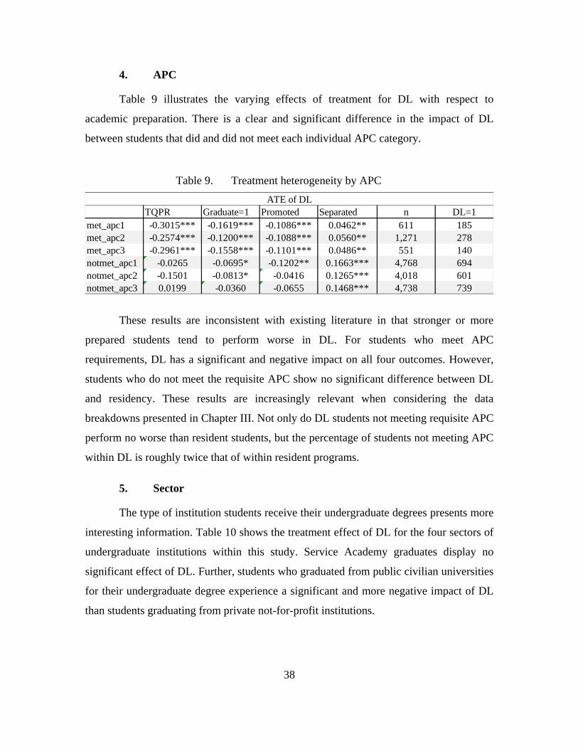
38

4. APC

Table 9 illustrates the varying effects of treatment for DL with respect to

academic preparation. There is a clear and significant difference in the impact of DL

between students that did and did not meet each individual APC category.

Table 9. Treatment heterogeneity by APC

These results are inconsistent with existing literature in that stronger or more

prepared students tend to perform worse in DL. For students who meet APC

requirements, DL has a significant and negative impact on all four outcomes. However,

students who do not meet the requisite APC show no significant difference between DL

and residency. These results are increasingly relevant when considering the data

breakdowns presented in Chapter III. Not only do DL students not meeting requisite APC

perform no worse than resident students, but the percentage of students not meeting APC

within DL is roughly twice that of within resident programs.

5. Sector

The type of institution students receive their undergraduate degrees presents more

interesting information. Table 10 shows the treatment effect of DL for the four sectors of

undergraduate institutions within this study. Service Academy graduates display no

significant effect of DL. Further, students who graduated from public civilian universities

for their undergraduate degree experience a significant and more negative impact of DL

than students graduating from private not-for-profit institutions.

TQPR Graduate=1 Promoted Separated n DL=1met_apc1 -0.3015*** -0.1619*** -0.1086*** 0.0462** 611 185met_apc2 -0.2574*** -0.1200*** -0.1088*** 0.0560** 1,271 278met_apc3 -0.2961*** -0.1558*** -0.1101*** 0.0486** 551 140notmet_apc1 -0.0265 -0.0695* -0.1202** 0.1663*** 4,768 694notmet_apc2 -0.1501 -0.0813* -0.0416 0.1265*** 4,018 601notmet_apc3 0.0199 -0.0360 -0.0655 0.1468*** 4,738 739

ATE of DL

39

Table 10. Treatment heterogeneity by sector

It is also interesting to see that Service Academy graduates experience the greatest

decrease in probability of promotion and the largest increase in probability of separation

as a result of DL. Students from public civilian institutions have a similar impact of DL

on promotion and separation; however, the magnitude is roughly half that of Service

Academy graduates.

6. School

Schools within NPS also present some interesting heterogeneity. Table 11 shows

treatment effects of DL for the four schools. GSEAS and GSOIS show similarly negative

impacts for DL with respect to both TQPR and probability of graduation. They differ

with respect to late graduation, however. DL actually has a significant and slightly

positive effect on the probability of graduating on time within GSOIS. More relevant,

however, is that students within GSBPP show no significant difference between DL and

residency on all outcomes except the probability of graduation.

Table 11. Treatment heterogeneity by school

TQPR Graduate=1 Promoted Separated n DL=1Public -0.3541*** -0.1565*** -0.0880** 0.0695** 2,679 363PrivateNFP -0.1921*** -0.1524*** -0.0666 0.0418 1,123 186PrivateFP 0.1093 -0.1509 -0.1796 -0.0101 43 4Service Academ -0.0727* -0.0591* -0.1456*** 0.1432*** 1,435 324

ATE of DL

TQPR Graduate=1 Promoted Separated n DL=1GSBPP -0.0982 -0.1114*** -0.0424 0.0264 1,477 555GSEAS -0.2147*** -0.1107*** -0.0508 0.0760* 1,099 203GSOIS -0.7181*** -0.2646*** -0.1691*** 0.0437 1,509 119SIGS 0.0981** 0.2404*** -0.4227*** 0.7918*** 1,086 2

ATE of DL

40


41

V. SUMMARY AND CONCLUSIONS

A. SUMMARY

I merge data from three separate sources to create a robust sample of NPS military

officer students. These data contain sound and diverse demographic and undergraduate

institution information. Using these diverse controls and employing propensity score

matching, I mitigate the pervasive issues present within the existing literature addressing

observational studies, small sample sizes, and demographic controls.

Utilizing the matched sample I find that DL has a significant and negative impact

on both student academic performance and subsequent job performance. Based on the

findings of existing literature, NPS students seem to be worse off than civilian

equivalents. Further, results are heterogeneous within different military services, warfare

communities, and levels of academic preparation.

B. RECOMMENDATIONS

When looking at the results, several potential means of improving the impact of

DL come to mind. First, focusing on programs or students who are more likely to

perform well in DL could help mitigate the existing negative impact on performance. For

example, students within GSBPP show no significant difference in performance between

DL and residency. With regard to warfare communities, Aviators suffer no significant

impact of DL as well. However, it is worth noting that several of these student

characteristics that tend to favor DL are already heavily represented within the existing

DL population. More than half of the students within the sample are already enrolled in

programs within GSBPP. Also, more than half of all DL students between 2006 and 2013

are Aviators. Thus, due to the existing makeup of DL, this solution may not be entirely

feasible.

Another area of potential improvement revolves around APC requirements. I

recommend creating less stringent requirements for admission to DL, or simply

continuing to waive existing requirements. Chapter III clearly demonstrated the large

number of students within DL who do not meet requisite APC values for their

42

curriculums. This observation is even more relevant when coupled with the

heterogeneous findings that students who do meet requisite APC suffer a significantly

negative impact of DL while those that do not meet requisite APC show no significant

effect of DL. Waiving APC requirements within DL does not seem to be manifesting any

significantly negative effect on students’ grades.

Next, I recommend shifting DL at NPS to a more asynchronous format. Although

there are asynchronous aspects of classes within NPS DL programs, they are primarily

synchronous in their delivery. The existing literature clearly addresses the superiority of

asynchronous formats over synchronous formats with regard to DL. Further, as most of

the studies that find no significant difference between distance and traditional formats are

based on asynchronous online programs, this difference in format could help explain the

uncharacteristically negative impact of DL at NPS.

Finally, I recommend conducting additional research on the impact of DL at NPS.

Particularly, the ability to control for individual course grades seems a logical next step.

The majority of existing literature focusses on individual courses and their associated

course grades when determining the impact of DL. As such, utilizing similar performance

outcomes could provide a better comparison to civilian equivalents.

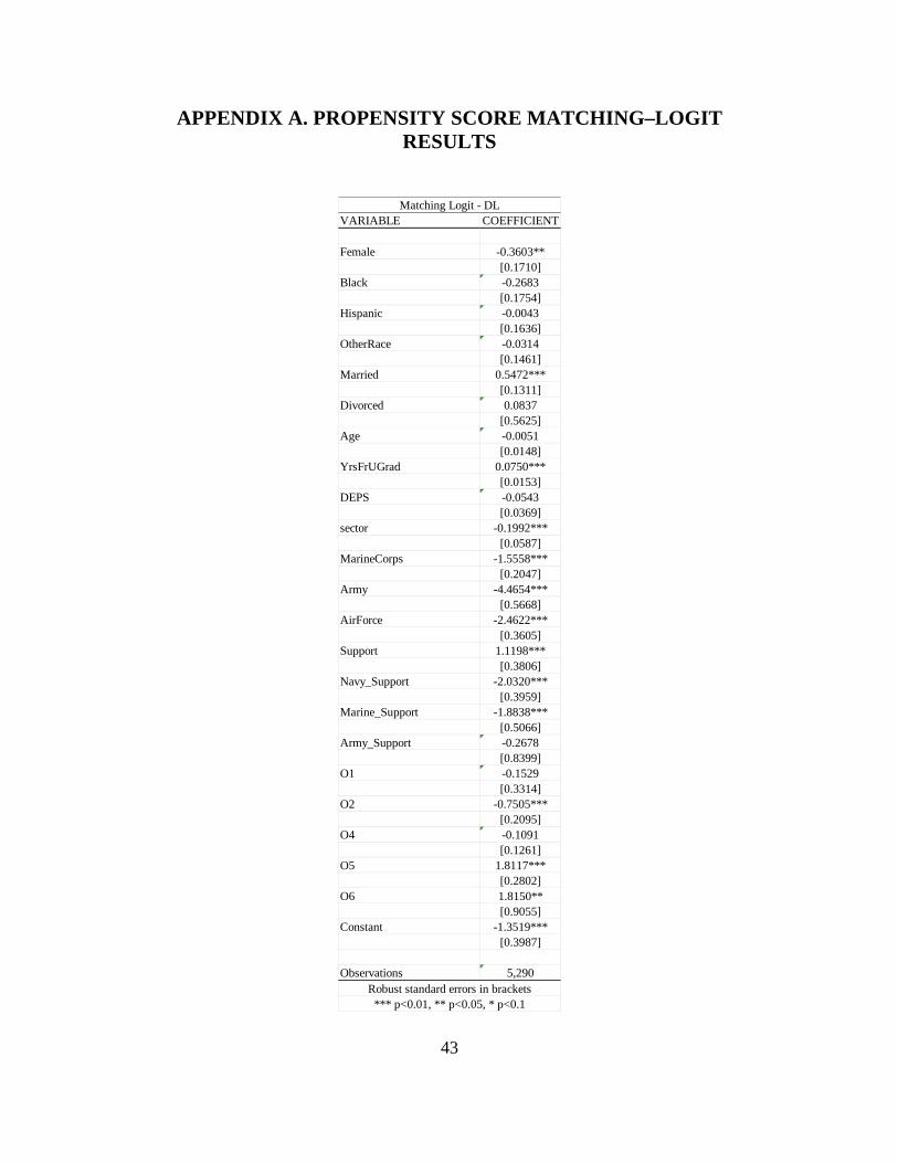
43

APPENDIX A. PROPENSITY SCORE MATCHING–LOGIT RESULTS

VARIABLE COEFFICIENT

Female -0.3603**[0.1710]

Black -0.2683[0.1754]

Hispanic -0.0043[0.1636]

OtherRace -0.0314[0.1461]

Married 0.5472***[0.1311]

Divorced 0.0837[0.5625]

Age -0.0051[0.0148]

YrsFrUGrad 0.0750***[0.0153]

DEPS -0.0543[0.0369]

sector -0.1992***[0.0587]

MarineCorps -1.5558***[0.2047]

Army -4.4654***[0.5668]

AirForce -2.4622***[0.3605]

Support 1.1198***[0.3806]

Navy_Support -2.0320***[0.3959]

Marine_Support -1.8838***[0.5066]

Army_Support -0.2678[0.8399]

O1 -0.1529[0.3314]

O2 -0.7505***[0.2095]

O4 -0.1091[0.1261]

O5 1.8117***[0.2802]

O6 1.8150**[0.9055]

Constant -1.3519***[0.3987]

Observations 5,290Robust standard errors in brackets*** p<0.01, ** p<0.05, * p<0.1

Matching Logit - DL

44


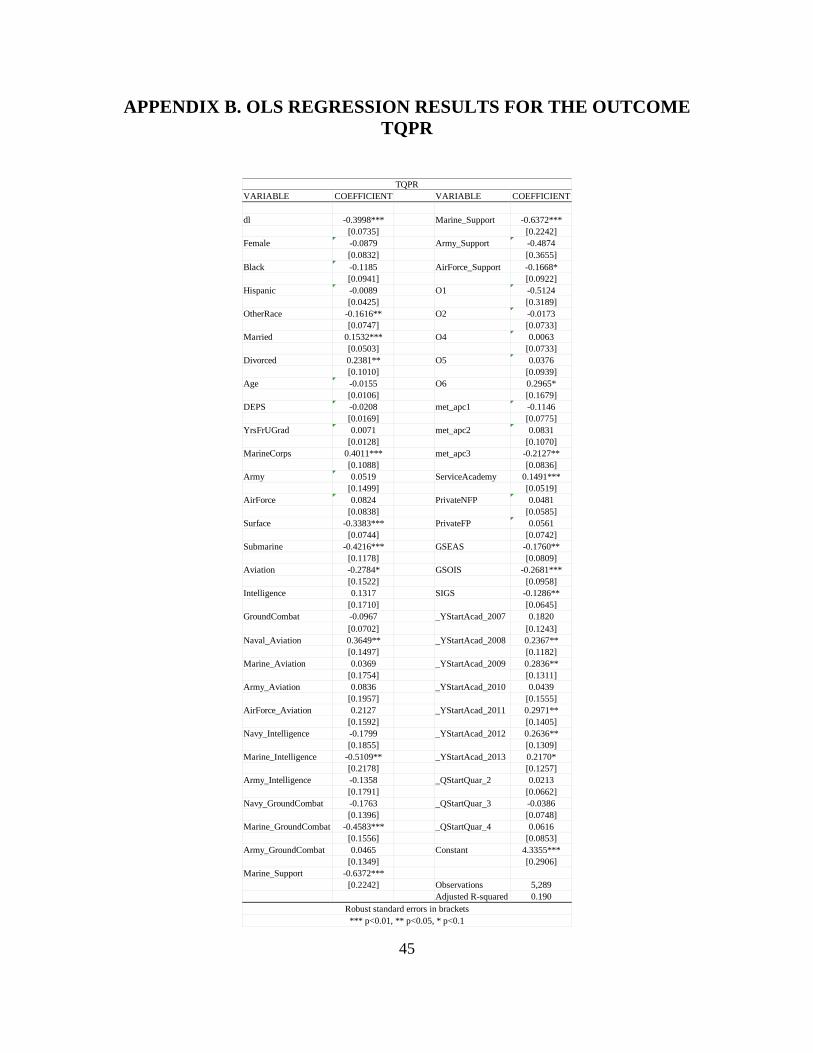
45

APPENDIX B. OLS REGRESSION RESULTS FOR THE OUTCOME TQPR

VARIABLE COEFFICIENT VARIABLE COEFFICIENT

dl -0.3998*** Marine_Support -0.6372***[0.0735] [0.2242]

Female -0.0879 Army_Support -0.4874[0.0832] [0.3655]

Black -0.1185 AirForce_Support -0.1668*[0.0941] [0.0922]

Hispanic -0.0089 O1 -0.5124[0.0425] [0.3189]

OtherRace -0.1616** O2 -0.0173[0.0747] [0.0733]

Married 0.1532*** O4 0.0063[0.0503] [0.0733]

Divorced 0.2381** O5 0.0376[0.1010] [0.0939]

Age -0.0155 O6 0.2965*[0.0106] [0.1679]

DEPS -0.0208 met_apc1 -0.1146[0.0169] [0.0775]

YrsFrUGrad 0.0071 met_apc2 0.0831[0.0128] [0.1070]

MarineCorps 0.4011*** met_apc3 -0.2127**[0.1088] [0.0836]

Army 0.0519 ServiceAcademy 0.1491***[0.1499] [0.0519]

AirForce 0.0824 PrivateNFP 0.0481[0.0838] [0.0585]

Surface -0.3383*** PrivateFP 0.0561[0.0744] [0.0742]

Submarine -0.4216*** GSEAS -0.1760**[0.1178] [0.0809]

Aviation -0.2784* GSOIS -0.2681***[0.1522] [0.0958]

Intelligence 0.1317 SIGS -0.1286**[0.1710] [0.0645]

GroundCombat -0.0967 _YStartAcad_2007 0.1820[0.0702] [0.1243]

Naval_Aviation 0.3649** _YStartAcad_2008 0.2367**[0.1497] [0.1182]

Marine_Aviation 0.0369 _YStartAcad_2009 0.2836**[0.1754] [0.1311]

Army_Aviation 0.0836 _YStartAcad_2010 0.0439[0.1957] [0.1555]

AirForce_Aviation 0.2127 _YStartAcad_2011 0.2971**[0.1592] [0.1405]

Navy_Intelligence -0.1799 _YStartAcad_2012 0.2636**[0.1855] [0.1309]

Marine_Intelligence -0.5109** _YStartAcad_2013 0.2170*[0.2178] [0.1257]

Army_Intelligence -0.1358 _QStartQuar_2 0.0213[0.1791] [0.0662]

Navy_GroundCombat -0.1763 _QStartQuar_3 -0.0386[0.1396] [0.0748]

Marine_GroundCombat -0.4583*** _QStartQuar_4 0.0616[0.1556] [0.0853]

Army_GroundCombat 0.0465 Constant 4.3355***[0.1349] [0.2906]

Marine_Support -0.6372***[0.2242] Observations 5,289

Adjusted R-squared 0.190Robust standard errors in brackets

TQPR

*** p<0.01, ** p<0.05, * p<0.1

46


47

APPENDIX C. LPM REGRESSION RESULTS FOR THE OUTCOME GRADUATE


dl -0.2232*** Marine_Support -0.2033**[0.0272] [0.1034]

Female -0.0402 Army_Support 0.0775[0.0395] [0.1547]

Black -0.1105** AirForce_Support -0.2313***[0.0508] [0.0553]

Hispanic -0.0877 O1 0.0037[0.0570] [0.0949]

OtherRace -0.0490 O2 0.0617[0.0327] [0.0421]

Married 0.0461 O4 -0.0071[0.0310] [0.0276]

Divorced 0.0540 O5 -0.1396***[0.0494] [0.0534]

Age -0.0039 O6 0.1984[0.0035] [0.1250]

DEPS -0.0116 met_apc1 -0.0613*[0.0086] [0.0336]

YrsFrUGrad 0.0005 met_apc2 0.0688**[0.0038] [0.0345]

MarineCorps 0.0630 met_apc3 -0.0861**[0.0884] [0.0373]

Army -0.1442 ServiceAcademy 0.0331[0.1253] [0.0204]

AirForce 0.0850* PrivateNFP -0.0052[0.0465] [0.0261]

Surface -0.1457*** PrivateFP -0.0906[0.0296] [0.1429]

Submarine -0.2015*** GSEAS -0.1128***[0.0370] [0.0296]

Aviation 0.0487 GSOIS -0.0981***[0.0803] [0.0298]

Intelligence -0.0344 SIGS -0.0446[0.0722] [0.0277]

GroundCombat -0.0621 _YStartAcad_2007 -0.0039[0.0473] [0.0369]

Naval_Aviation -0.0465 _YStartAcad_2008 0.0199[0.0826] [0.0353]

Marine_Aviation -0.0563 _YStartAcad_2009 0.0301[0.1189] [0.0414]

Army_Aviation -0.0966 _YStartAcad_2010 -0.0384[0.1303] [0.0432]

AirForce_Aviation -0.1370* _YStartAcad_2011 -0.0026[0.0804] [0.0414]

Navy_Intelligence -0.0081 _YStartAcad_2012 -0.0903**[0.0793] [0.0403]

Marine_Intelligence -0.0172 _YStartAcad_2013 -0.6134***[0.1304] [0.0383]

Army_Intelligence 0.0831 _QStartQuar_2 -0.0254[0.0908] [0.0268]

Navy_GroundCombat -0.0194 _QStartQuar_3 -0.0831***[0.0612] [0.0311]

Marine_GroundCombat -0.1658 _QStartQuar_4 -0.1225***[0.1376] [0.0298]

Army_GroundCombat 0.2331** Constant 1.3504***[0.1181] [0.1157]

Observations 5,289Adjusted R-squared 0.364

Robust standard errors in brackets*** p<0.01, ** p<0.05, * p<0.1

GRADUATE

48


49

APPENDIX D. LPM REGRESSION RESULTS FOR THE OUTCOME PROMOTED


dl -0.1253*** Marine_Support -0.3884***[0.0276] [0.0769]

Female -0.0157 Army_Support -0.0272[0.0484] [0.0788]

Black -0.0408 AirForce_Support -0.2065[0.0374] [0.1262]

Hispanic -0.0138 O1 0.2753***[0.0379] [0.0958]

OtherRace -0.0435 O2 -0.1268***[0.0292] [0.0390]

Married 0.0846*** O4 -0.0873***[0.0307] [0.0287]

Divorced 0.0514 O5 -0.4005***[0.0698] [0.0460]

Age -0.0101*** O6 -0.2171**[0.0036] [0.0964]

DEPS -0.0104 met_apc1 0.0058[0.0085] [0.0407]

YrsFrUGrad 0.0018 met_apc2 0.0233[0.0041] [0.0255]

MarineCorps 0.2038*** met_apc3 -0.0111[0.0647] [0.0396]

Army -0.1308* ServiceAcademy 0.0022[0.0683] [0.0223]

AirForce 0.0739 PrivateNFP 0.0016[0.1270] [0.0263]

Surface -0.2172*** PrivateFP 0.0727[0.0302] [0.0660]

Submarine -0.0764* GSEAS -0.0628**[0.0404] [0.0296]

Aviation -0.9628*** GSOIS -0.0736***[0.2008] [0.0245]

Intelligence -0.1469 SIGS 0.0349[0.1739] [0.0236]

GroundCombat 0.1565 _YStartAcad_2007 -0.0345[0.1832] [0.0450]

Naval_Aviation 0.8828*** _YStartAcad_2008 -0.0930**[0.2001] [0.0416]

Marine_Aviation 0.6711*** _YStartAcad_2009 -0.2989***[0.2160] [0.0425]

Army_Aviation 0.9687*** _YStartAcad_2010 -0.3362***[0.2136] [0.0431]

AirForce_Aviation 1.1520*** _YStartAcad_2011 -0.4546***[0.2398] [0.0365]

Navy_Intelligence -0.0653 _YStartAcad_2012 -0.5902***[0.1778] [0.0340]


Army_Intelligence 0.1968 _QStartQuar_2 -0.0675***[0.1782] [0.0255]

Navy_GroundCombat -0.1288 _QStartQuar_3 -0.0176[0.1880] [0.0277]

Marine_GroundCombat -0.5448*** _QStartQuar_4 -0.1001***[0.1983] [0.0256]

Army_GroundCombat -0.1518 Constant 1.2456***[0.1930] [0.1198]


*** p<0.01, ** p<0.05, * p<0.1Robust standard errors in brackets

PROMOTED

50


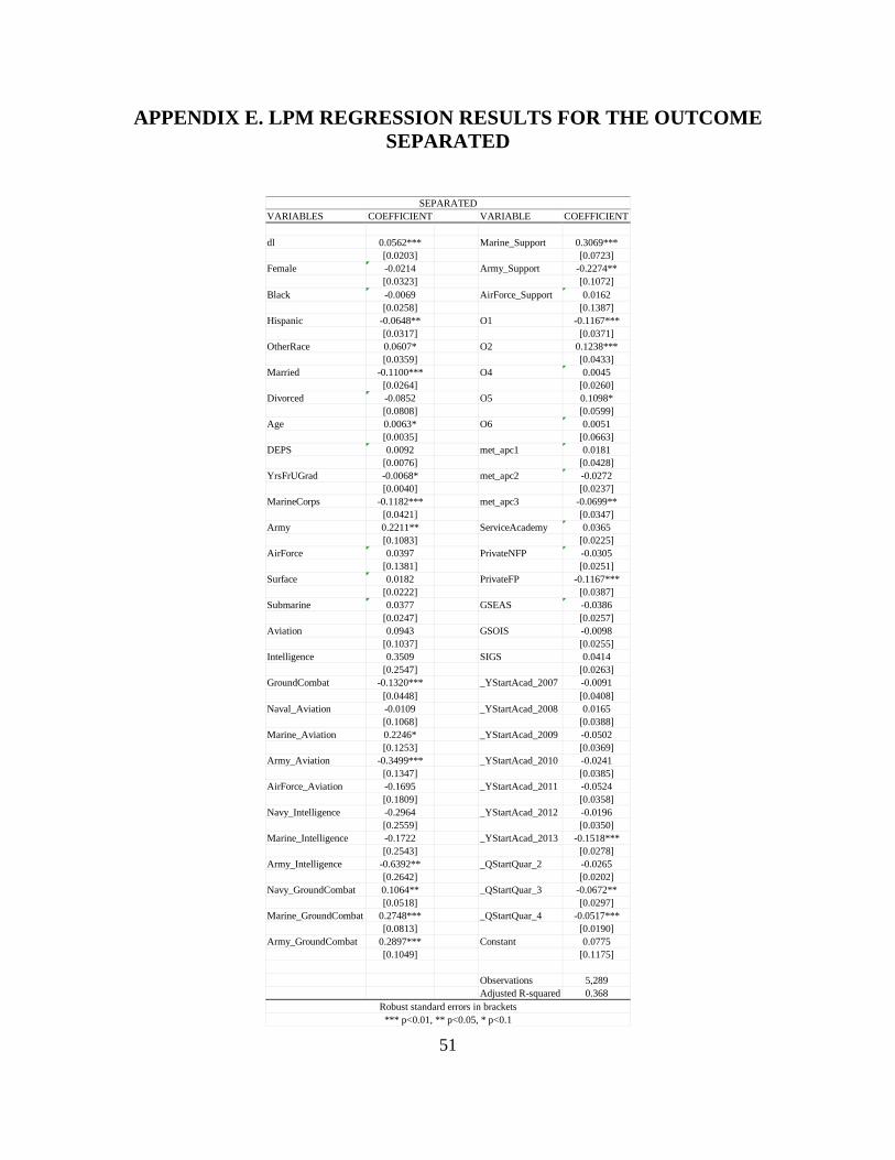
51

APPENDIX E. LPM REGRESSION RESULTS FOR THE OUTCOME SEPARATED

VARIABLES COEFFICIENT VARIABLE COEFFICIENT

dl 0.0562*** Marine_Support 0.3069***[0.0203] [0.0723]

Female -0.0214 Army_Support -0.2274**[0.0323] [0.1072]

Black -0.0069 AirForce_Support 0.0162[0.0258] [0.1387]

Hispanic -0.0648** O1 -0.1167***[0.0317] [0.0371]

OtherRace 0.0607* O2 0.1238***[0.0359] [0.0433]

Married -0.1100*** O4 0.0045[0.0264] [0.0260]

Divorced -0.0852 O5 0.1098*[0.0808] [0.0599]

Age 0.0063* O6 0.0051[0.0035] [0.0663]

DEPS 0.0092 met_apc1 0.0181[0.0076] [0.0428]

YrsFrUGrad -0.0068* met_apc2 -0.0272[0.0040] [0.0237]

MarineCorps -0.1182*** met_apc3 -0.0699**[0.0421] [0.0347]

Army 0.2211** ServiceAcademy 0.0365[0.1083] [0.0225]

AirForce 0.0397 PrivateNFP -0.0305[0.1381] [0.0251]

Surface 0.0182 PrivateFP -0.1167***[0.0222] [0.0387]

Submarine 0.0377 GSEAS -0.0386[0.0247] [0.0257]

Aviation 0.0943 GSOIS -0.0098[0.1037] [0.0255]

Intelligence 0.3509 SIGS 0.0414[0.2547] [0.0263]

GroundCombat -0.1320*** _YStartAcad_2007 -0.0091[0.0448] [0.0408]

Naval_Aviation -0.0109 _YStartAcad_2008 0.0165[0.1068] [0.0388]

Marine_Aviation 0.2246* _YStartAcad_2009 -0.0502[0.1253] [0.0369]

Army_Aviation -0.3499*** _YStartAcad_2010 -0.0241[0.1347] [0.0385]

AirForce_Aviation -0.1695 _YStartAcad_2011 -0.0524[0.1809] [0.0358]

Navy_Intelligence -0.2964 _YStartAcad_2012 -0.0196[0.2559] [0.0350]


Army_Intelligence -0.6392** _QStartQuar_2 -0.0265[0.2642] [0.0202]

Navy_GroundCombat 0.1064** _QStartQuar_3 -0.0672**[0.0518] [0.0297]

Marine_GroundCombat 0.2748*** _QStartQuar_4 -0.0517***[0.0813] [0.0190]

Army_GroundCombat 0.2897*** Constant 0.0775[0.1049] [0.1175]


*** p<0.01, ** p<0.05, * p<0.1Robust standard errors in brackets

SEPARATED

52


53

APPENDIX F. OLS REGRESSION RESULTS FOR THE OUTCOME TQPR—HETEROGENEITY

AT

ESE

Coe

f.S

EC

oef.

SE

Coe

f.SE

Coe

f.S

EC

oef.

SE

Coe

f.SE

Coe

f.S

EC

oef.

SEC

oef.

SE

Nav

y-0

.164

7***

[0.0

366]

-0.1

289

[0.1

087]

-0.2

051*

**[0

.072

4]-0

.053

9[0

.044

2]-0

.188

3*[0

.104

1]0.

2269

***

[0.0

583]

-0.0

099

[0.0

066]

-0.0

339*

[0.0

178]

0.01

99**

*[0

.006

6]30

5577

6M

arin

eCor

ps-0

.261

6[0

.163

0]0.

1632

[0.1

690]

-0.1

708

[0.1

480]

0.05

13[0

.147

0]-0

.303

7[0

.416

9]-0

.021

1[0

.241

4]0.

2666

[0.2

420]

-0.0

744

[0.0

678]

0.06

95[0

.069

8]0.

0861

[0.0

570]

684

41A

rmy

-0.8

085

[0.7

273]

-0.3

110

[0.2

373]

0.54

84[0

.557

4]0.

1948

[0.3

336]

0.30

12[0

.376

0]-0

.017

1[0

.204

7]-0

.129

1[0

.273

2]-0

.048

7*[0

.026

3]-0

.066

1[0

.054

4]0.

0173

*[0

.009

8]75

57

Air

For

ce-0

.183

3***

[0.0

610]

-0.1

033

[0.1

496]

-0.2

638

[0.2

357]

0.03

56[0

.203

1]-0

.058

1[0

.132

4]0.

0920

[0.1

934]

0.00

41[0

.181

9]0.

0160

[0.0

103]

-0.0

461

[0.0

366]

0.00

49[0

.010

6]75

455

Surf

ace

-0.5

322*

**[0

.175

1]-0

.480

7**

[0.2

337]

-0.2

883*

*[0

.138

8]0.

1364

[0.1

224]

-0.3

712

[0.2

537]

0.18

29**

[0.0

901]

0.00

08[0

.013

0]-0

.099

4*[0

.051

1]0.

0128

[0.0

224]

695

68S

ubm

arin

e-1

.218

9***

[0.2

965]

0.75

99**

[0.3

230]

-0.8

993*

*[0

.416

9]-0

.180

3[0

.361

2]0.

0567

[0.3

558]

0.79

38**

[0.3

397]

0.02

24[0

.034

3]-0

.037

4[0

.088

9]-0

.024

8[0

.036

9]23

051

Avi

atio

n-0

.064

6***

[0.0

237]

0.04

97[0

.048

6]-0

.052

8[0

.064

4]0.

0136

[0.0

311]

-0.0

742

[0.0

928]

0.03

57[0

.048

2]0.

1584

**[0

.064

6]-0

.010

4***

[0.0

035]

0.01

70*

[0.0

100]

0.00

46[0

.003

7]11

6451

2In

telli

genc

e-0

.458

0[0

.413

3]-0

.492

2[0

.334

0]-0

.229

7***

[0.0

771]

0.04

44[0

.149

9]-0

.511

1[0

.322

6]0.

0254

[0.1

401]

0.15

63[0

.180

4]-0

.001

4[0

.007

9]-0

.020

1[0

.027

8]0.

0133

**[0

.005

3]59

013

Gro

undC

omba

t-0

.452

0**

[0.2

221]

-1.0

034

[0.7

323]

-0.0

373

[0.1

505]

0.24

71[0

.169

1]0.

1910

[0.1

920]

0.04

91[0

.112

2]-0

.026

6[0

.136

7]-0

.019

1**

[0.0

082]

-0.0

243

[0.0

232]

0.00

93[0

.007

3]68

418

Supp

ort

-0.3

375*

*[0

.132

0]0.

0818

[0.0

958]

-0.0

020

[0.1

441]

0.02

98[0

.103

7]-0

.041

7[0

.146

9]0.

1614

[0.1

156]

0.26

01**

[0.1

315]

-0.0

224

[0.0

236]

-0.0

317

[0.0

327]

0.01

82[0

.027

2]21

3120

7O

1-1

.051

1[0

.646

9]-0

.016

6[0

.123

9]-0

.211

5[0

.351

1]0.

2368

[0.1

820]

0.30

16[0

.480

7]1.

5130

*[0

.793

8]-0

.103

2[0

.169

3]-0

.380

1[0

.373

0]-0

.031

7[0

.146

6]12

313

O2

-0.1

901*

[0.1

050]

-0.7

921*

*[0

.381

7]-0

.500

5**

[0.2

108]

-0.0

225

[0.1

039]

-0.1

585

[0.1

578]

0.25

15*

[0.1

323]

-0.0

890

[0.1

635]

-0.0

091

[0.0

168]

-0.2

148*

**[0

.082

2]0.

0045

[0.0

246]

438

29O

3-0

.143

0***

[0.0

443]

-0.0

605

[0.0

905]

-0.2

207*

*[0

.088

4]-0

.080

5[0

.061

2]-0

.132

8[0

.128

0]0.

1319

*[0

.072

3]0.

2875

***

[0.0

750]

-0.0

115

[0.0

086]

-0.0

085

[0.0

174]

0.01

37[0

.009

0]29

5053

0O

4-0

.317

3*[0

.185

0]0.

1302

[0.0

915]

0.05

14[0

.177

6]0.

0727

[0.1

305]

0.07

66[0

.142

8]0.

0017

[0.0

638]

-0.2

475*

[0.1

290]

-0.0

494

[0.0

310]

-0.0

161

[0.0

188]

0.02

94[0

.031

4]16

0419

8O

5-0

.210

4**

[0.1

050]

-0.5

805

[0.5

339]

-0.6

366

[0.5

643]

0.06

80[0

.099

7]-0

.241

3[0

.355

2]0.

1007

[0.1

345]

-0.0

181

[0.0

196]

-0.0

168

[0.0

336]

-0.0

074

[0.0

111]

139

100

O6

-0.1

747

[0.0

933]

0.13

28[0

.063

3]0.

0149

[0.0

625]

0.09

05[0

.093

4]-0

.121

0[0

.058

7]-0

.006

8[0

.006

2]0.

0368

[0.0

232]

0.01

37[0

.006

8]11

9m

et_a

pc1

-0.3

015*

**[0

.083

8]-0

.062

7[0

.094

7]-0

.144

6*[0

.075

1]0.

0138

[0.0

583]

-0.1

757

[0.1

188]

0.19

45**

*[0

.075

2]0.

2573

**[0

.113

5]-0

.017

9[0

.017

7]-0

.034

0*[0

.018

8]0.

0253

[0.0

181]

611

185

met

_apc

2-0

.257

4***

[0.0

706]

-0.1

463

[0.1

150]

-0.1

142*

[0.0

658]

-0.0

419

[0.0

560]

-0.2

526*

[0.1

343]

0.17

15**

[0.0

763]

0.27

43**

*[0

.099

9]-0

.026

1[0

.024

1]-0

.012

0[0

.017

2]0.

0413

*[0

.022

4]12

7127

8m

et_a

pc3

-0.2

961*

**[0

.080

5]-0

.044

3[0

.094

5]-0

.121

0[0

.077

1]0.

0087

[0.0

576]

-0.1

633

[0.1

169]

0.20

54**

*[0

.076

4]0.

2807

**[0

.110

9]-0

.021

9[0

.017

4]-0

.026

3[0

.017

8]0.

0294

*[0

.017

7]55

114

0no

tmet

_apc

1-0

.026

5[0

.043

4]-0

.230

9[0

.171

7]-0

.252

9[0

.171

1]-0

.088

5[0

.141

0]0.

0304

[0.0

863]

0.16

92**

[0.0

786]

0.35

29**

*[0

.131

9]-0

.013

5[0

.010

0]-0

.026

8[0

.029

4]0.

0170

**[0

.008

5]47

6869

4no

tmet

_apc

2-0

.150

1[0

.109

8]0.

0245

[0.1

129]

-0.1

925

[0.1

827]

0.06

33[0

.109

6]0.

1385

[0.0

898]

0.21

93**

[0.0

943]

0.10

84[0

.178

5]-0

.005

6[0

.010

2]-0

.060

5*[0

.031

9]-0

.008

5[0

.019

3]40

1860

1no

tmet

_apc

30.

0199

[0.0

431]

-0.2

583

[0.1

633]

-0.2

421

[0.1

908]

-0.0

590

[0.1

384]

0.00

20[0

.066

2]0.

1100

[0.0

779]

0.28

44*

[0.1

475]

0.00

17[0

.006

6]-0

.049

0[0

.030

6]0.

0054

[0.0

070]

4738

739

Publ

ic-0

.354

1***

[0.1

301]

-0.2

175

[0.1

804]

0.01

17[0

.119

8]0.

0281

[0.1

001]

-0.2

513

[0.1

793]

0.14

72[0

.101

7]0.

2369

[0.1

521]

-0.0

327

[0.0

253]

-0.0

226

[0.0

263]

0.02

96[0

.025

3]26

7936

3P

riva

teN

FP

-0.1

921*

**[0

.059

3]-0

.048

6[0

.129

1]-0

.245

0*[0

.140

3]0.

0739

[0.1

491]

-0.0

097

[0.0

994]

0.33

25**

*[0

.116

9]0.

3687

***

[0.1

037]

0.01

02[0

.007

5]-0

.067

4**

[0.0

280]

0.01

11[0

.007

2]11

2318

6P

riva

teF

P0.

1093

[0.0

758]

0.06

77[0

.110

5]-0

.337

9***

[0.1

127]

-0.3

066*

**[0

.111

1]-0

.178

1[0

.128

6]-0

.196

2[0

.130

7]-0

.010

4[0

.009

8]-0

.011

8[0

.040

8]0.

0065

[0.0

101]

434

Ser

vice

Aca

dem

y-0

.072

7*[0

.041

3]0.

0419

[0.0

429]

-0.3

930*

*[0

.190

2]-0

.038

7[0

.036

0]-0

.033

4[0

.061

2]-0

.041

8[0

.065

8]-0

.045

8[0

.066

4]-0

.003

9[0

.007

3]0.

0165

[0.0

153]

0.01

03[0

.007

4]14

3532

4G

SBPP

-0.0

982

[0.0

887]

0.04

93[0

.043

7]-0

.107

2[0

.078

9]0.

0288

[0.0

992]

0.01

18[0

.079

0]0.

1140

[0.0

729]

0.14

18[0

.153

5]-0

.025

8***

[0.0

072]

-0.0

278

[0.0

182]

0.01

01[0

.015

5]14

7755

5G

SEA

S-0

.214

7***

[0.0

685]

-0.2

322

[0.1

904]

-0.1

565

[0.1

436]

0.01

23[0

.163

5]-0

.065

4[0

.145

6]0.

2750

**[0

.124

6]0.

5923

***

[0.1

384]

0.01

29[0

.009

7]-0

.084

4**

[0.0

401]

0.00

77[0

.012

9]10

9920

3G

SO

IS-0

.718

1***

[0.1

782]

-0.4

034

[0.2

639]

-0.3

046*

*[0

.137

7]0.

1005

[0.0

940]

-0.6

231*

*[0

.250

7]-0

.045

8[0

.152

3]0.

1711

[0.1

630]

-0.0

575

[0.0

364]

0.02

86[0

.033

4]0.

0545

*[0

.032

9]15

0911

9SI

GS

0.09

81**

[0.0

473]

0.04

39*

[0.0

234]

-0.1

584*

**[0

.040

9]-0

.168

4***

[0.0

511]

-0.0

925*

*[0

.036

3]0.

0552

*[0

.032

4]0.

0115

[0.0

394]

-0.0

036

[0.0

030]

0.00

43[0

.008

8]0.

0086

**[0

.003

4]10

862

Dem

ogra

phic

Con

trol

sFe

mal

eB

lack

His

pani

cO

ther

Rac

eM

arri

edD

ivor

ced

Age

Tre

atm

ent H

eter

ogen

eity

- T

QP

R

VA

RIA

BL

E =

1D

EP

SY

rsFr

UG

rad

Tre

atm

ent

dln

DL

=1

Rob

ust s

tand

ard

erro

rs in

bra

cket

s**

* p<

0.01

, **

p<0.

05, *

p<

0.1

54


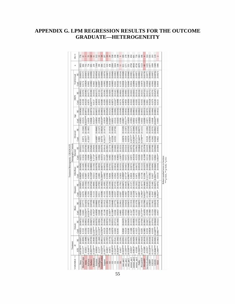
55

APPENDIX G. LPM REGRESSION RESULTS FOR THE OUTCOME GRADUATE—HETEROGENEITY

AT

ESE

Coe

f.SE

Coe

f.SE

Coe

f.SE

Coe

f.SE

Coe

f.SE

Coe

f.SE

Coe

f.SE

Coe

f.SE

Coe

f.SE

Nav

y-0

.077

8***

[0.0

207]

-0.0

553

[0.0

472]

-0.0

440

[0.0

431]

-0.0

257

[0.0

397]

-0.0

829*

[0.0

430]

0.02

72[0

.031

1]-0

.005

1[0

.003

6]-0

.011

0[0

.009

1]0.

0022

[0.0

037]

3055

776

Mar

ineC

orps

-0.2

122*

*[0

.089

9]0.

1510

[0.1

002]

0.04

83[0

.077

7]0.

0278

[0.0

969]

-0.0

955

[0.1

428]

0.16

34[0

.122

9]0.

0073

[0.2

360]

-0.0

125

[0.0

164]

-0.0

108

[0.0

370]

0.01

74[0

.013

7]68

441

Arm

y-0

.261

1[0

.169

8]-0

.150

2[0

.095

1]0.

3102

**[0

.142

5]-0

.098

3[0

.115

6]0.

1607

[0.1

069]

0.02

28[0

.073

0]-0

.017

7[0

.120

9]-0

.022

3***

[0.0

071]

-0.0

123

[0.0

190]

-0.0

029

[0.0

047]

755

7A

irFo

rce

-0.1

644*

**[0

.048

7]-0

.021

8[0

.090

4]-0

.625

8***

[0.0

875]

-0.2

301

[0.2

158]

-0.0

416

[0.1

093]

0.00

68[0

.096

8]-0

.320

2*[0

.186

3]0.

0039

[0.0

060]

0.00

76[0

.017

7]0.

0002

[0.0

062]

754

55Su

rfac

e-0

.283

7***

[0.0

729]

-0.0

363

[0.0

667]

-0.0

552

[0.0

729]

-0.0

630

[0.0

754]

-0.1

558*

[0.0

800]

0.09

05*

[0.0

546]

0.00

48[0

.007

3]-0

.047

7**

[0.0

198]

-0.0

082

[0.0

090]

695

68Su

bmar

ine

-0.5

338*

**[0

.084

8]0.

2258

***

[0.0

823]

-0.1

832*

[0.1

089]

-0.1

131

[0.0

808]

-0.0

213

[0.1

356]

0.17

14*

[0.0

929]

-0.0

215*

[0.0

112]

0.01

37[0

.033

4]0.

0065

[0.0

122]

230

51A

viat

ion

-0.0

014

[0.0

259]

0.13

27**

[0.0

570]

-0.0

058

[0.0

860]

0.03

18[0

.062

0]0.

0138

[0.0

579]

0.06

73[0

.043

9]0.

1600

*[0

.084

0]-0

.005

4[0

.005

7]-0

.001

9[0

.011

7]0.

0087

[0.0

054]

1164

512

Inte

llige

nce

-0.1

277

[0.1

468]

-0.2

130*

*[0

.089

4]0.

0448

[0.0

789]

0.05

11[0

.078

9]-0

.088

1[0

.085

0]0.

0084

[0.0

668]

0.08

83[0

.116

7]-0

.004

6[0

.006

1]-0

.003

3[0

.015

0]0.

0089

*[0

.005

2]59

013

Gro

undC

omba

t-0

.233

2**

[0.0

911]

-0.3

783*

*[0

.172

4]0.

0796

[0.1

002]

-0.0

386

[0.1

063]

0.23

84**

*[0

.067

7]-0

.037

2[0

.057

9]0.

0776

[0.0

824]

-0.0

154*

*[0

.006

3]0.

0188

[0.0

173]

0.00

49[0

.006

6]68

418

Supp

ort

-0.1

997*

**[0

.045

5]-0

.012

9[0

.058

4]-0

.114

0[0

.101

2]-0

.116

1[0

.109

9]-0

.068

2[0

.065

5]0.

0137

[0.0

614]

-0.3

613*

*[0

.147

1]-0

.003

9[0

.006

7]-0

.028

5[0

.019

6]-0

.000

2[0

.007

4]21

3120

7O

1-0

.281

7[0

.170

7]-0

.012

4[0

.057

2]0.

0336

[0.1

285]

-0.1

233

[0.2

753]

0.11

94[0

.165

6]0.

1429

[0.2

591]

-0.0

968*

[0.0

520]

0.03

93[0

.153

9]0.

0588

[0.0

467]

123

13O

2-0

.087

3[0

.077

8]-0

.139

4[0

.132

0]-0

.369

7*[0

.215

4]-0

.269

9[0

.233

8]0.

0646

[0.0

742]

0.00

83[0

.127

4]0.

2256

**[0

.101

4]-0

.026

8**

[0.0

121]

-0.0

033

[0.0

429]

0.00

18[0

.016

1]43

829

O3

-0.1

014*

**[0

.027

7]-0

.037

0[0

.055

1]-0

.118

6*[0

.064

8]-0

.038

9[0

.045

6]-0

.065

0[0

.055

7]0.

0342

[0.0

386]

-0.2

236

[0.1

836]

0.00

31[0

.004

8]-0

.007

1[0

.013

8]-0

.000

5[0

.004

9]29

5053

0O

4-0

.154

5***

[0.0

541]

-0.0

402

[0.0

713]

0.03

68[0

.077

5]-0

.035

7[0

.071

9]-0

.094

1[0

.083

4]0.

0491

[0.0

468]

-0.0

593

[0.0

768]

-0.0

141

[0.0

086]

-0.0

242*

[0.0

142]

0.00

41[0

.008

2]16

0419

8O

5-0

.353

4***

[0.1

094]

0.01

91[0

.195

0]-0

.053

3[0

.180

7]-0

.055

6[0

.167

8]-0

.254

5[0

.305

6]-0

.066

1[0

.192

2]-0

.024

1[0

.015

6]-0

.009

8[0

.038

9]0.

0126

[0.0

090]

139

100

O6

-0.4

017

[0.2

295]

0.48

65[0

.206

1]0.

0207

[0.1

781]

-0.5

831

[0.3

153]

-1.0

287*

[0.3

223]

0.05

08[0

.054

9]0.

0174

[0.0

826]

0.11

03[0

.052

4]11

9m

et_a

pc1

-0.1

619*

**[0

.029

1]0.

0040

[0.0

419]

-0.0

916

[0.0

592]

-0.0

099

[0.0

407]

-0.0

890*

[0.0

455]

0.04

16[0

.035

4]-0

.067

6[0

.152

9]-0

.006

7[0

.004

8]-0

.007

6[0

.010

6]0.

0038

[0.0

048]

611

185

met

_apc

2-0

.120

0***

[0.0

261]

-0.0

229

[0.0

447]

-0.0

542

[0.0

424]

-0.0

467

[0.0

418]

-0.0

774*

[0.0

441]

0.03

72[0

.032

4]-0

.091

9[0

.158

7]-0

.011

7**

[0.0

056]

0.00

58[0

.009

0]0.

0102

*[0

.005

3]12

7127

8m

et_a

pc3

-0.1

558*

**[0

.027

9]0.

0100

[0.0

419]

-0.0

881

[0.0

567]

-0.0

158

[0.0

407]

-0.0

807*

[0.0

448]

0.04

75[0

.035

2]-0

.057

4[0

.151

0]-0

.005

9[0

.004

6]-0

.005

6[0

.010

3]0.

0049

[0.0

046]

551

140

notm

et_a

pc1

-0.0

695*

[0.0

395]

-0.1

488

[0.1

213]

-0.1

627

[0.1

353]

-0.3

443

[0.2

137]

0.08

18[0

.067

2]0.

0072

[0.0

879]

-0.4

575*

*[0

.211

7]-0

.000

4[0

.006

8]-0

.024

3[0

.026

3]0.

0024

[0.0

081]

4768

694

notm

et_a

pc2

-0.0

813*

[0.0

429]

-0.0

576

[0.0

838]

-0.1

230

[0.1

316]

-0.1

358

[0.1

533]

0.10

30[0

.076

6]-0

.015

4[0

.077

8]-0

.416

6**

[0.2

049]

0.00

32[0

.006

1]-0

.036

5[0

.026

3]-0

.009

6[0

.007

7]40

1860

1no

tmet

_apc

3-0

.036

0[0

.046

9]-0

.162

5[0

.119

5]-0

.116

2[0

.167

8]-0

.347

7[0

.236

3]0.

0471

[0.0

637]

-0.0

333

[0.0

962]

-0.5

751*

**[0

.169

9]-0

.003

1[0

.008

1]-0

.028

2[0

.031

4]0.

0013

[0.0

097]

4738

739

Publ

ic-0

.156

5***

[0.0

401]

-0.1

121*

[0.0

574]

0.03

21[0

.060

7]0.

0497

[0.0

514]

-0.0

666

[0.0

519]

0.03

26[0

.046

4]0.

1441

**[0

.067

7]-0

.008

8[0

.006

2]-0

.011

3[0

.013

4]0.

0089

[0.0

061]

2679

363

Priv

ateN

FP-0

.152

4***

[0.0

424]

0.02

95[0

.076

0]-0

.277

9**

[0.1

155]

-0.2

984*

[0.1

677]

-0.1

736

[0.1

122]

0.01

64[0

.075

6]-0

.579

8***

[0.1

251]

0.00

32[0

.005

5]-0

.010

2[0

.021

5]-0

.007

6[0

.005

2]11

2318

6Pr

ivat

eFP

-0.1

509

[0.2

019]

0.24

83[0

.206

1]-0

.247

8[0

.278

0]0.

4321

*[0

.246

4]0.

1394

[0.2

337]

-0.1

549

[0.2

374]

0.02

99[0

.021

3]0.

0385

[0.0

712]

0.01

07[0

.017

6]43

4Se

rvic

eAca

dem

y-0

.059

1*[0

.030

2]0.

0250

[0.0

467]

-0.0

586

[0.0

821]

-0.1

108*

[0.0

640]

0.12

11**

*[0

.046

8]0.

0114

[0.0

419]

0.01

28[0

.108

4]-0

.007

1[0

.007

0]0.

0061

[0.0

161]

-0.0

040

[0.0

077]

1435

324

GSB

PP-0

.111

4***

[0.0

334]

-0.0

628

[0.0

677]

-0.1

060

[0.0

672]

-0.0

832

[0.0

723]

-0.1

302

[0.0

792]

0.03

49[0

.049

9]-0

.378

4[0

.251

9]-0

.005

9[0

.005

5]-0

.012

4[0

.017

1]0.

0052

[0.0

065]

1477

555

GSE

AS

-0.1

107*

**[0

.041

4]-0

.010

5[0

.079

3]-0

.153

4[0

.158

2]-0

.204

7[0

.154

8]0.

0457

[0.0

696]

0.01

53[0

.074

8]-0

.266

2[0

.357

0]0.

0048

[0.0

084]

-0.0

379

[0.0

276]

-0.0

042

[0.0

097]

1099

203

GSO

IS-0

.264

6***

[0.0

585]

-0.1

407*

*[0

.066

4]-0

.045

8[0

.061

9]0.

0885

[0.0

637]

-0.2

061*

**[0

.066

0]0.

0061

[0.0

592]

0.01

60[0

.096

3]-0

.016

3**

[0.0

081]

0.01

28[0

.014

7]0.

0060

[0.0

076]

1509

119

SIG

S0.

2404

***

[0.0

463]

0.08

81**

*[0

.032

2]-0

.005

7[0

.052

4]-0

.095

3**

[0.0

476]

-0.0

110

[0.0

354]

0.08

10**

[0.0

384]

0.08

22[0

.059

3]0.

0003

[0.0

032]

0.01

33[0

.009

2]0.

0010

[0.0

027]

1086

2

VA

RIA

BL

E =

1T

reat

men

tD

emog

raph

ic C

ontr

ols

dlA

geD

EPS

Yrs

FrU

Gra

dFe

mal

eB

lack

His

pani

cO

ther

Rac

eM

arri

edD

ivor

ced

nD

L=

1

Tre

atm

ent H

eter

ogen

eity

- G

RA

DU

AT

E

Rob

ust s

tand

ard

erro

rs in

bra

cket

s**

* p<

0.01

, **

p<0.

05, *

p<

0.1

56


57

APPENDIX H. LPM REGRESSION RESULTS FOR THE OUTCOME PROMOTED—HETEROGENEITY

AT

ES

EC

oef.

SEC

oef.

SEC

oef.

SE

Coe

f.S

EC

oef.

SEC

oef.

SE

Coe

f.S

EC

oef.

SEC

oef.

SE

Nav

y0.

0477

**[0

.024

1]-0

.045

5[0

.053

9]-0

.012

1[0

.051

3]-0

.002

5[0

.042

3]-0

.054

3[0

.046

1]0.

0067

[0.0

373]

-0.0

115*

*[0

.004

7]-0

.001

8[0

.010

8]-0

.016

2***

[0.0

044]

3055

776

Mar

ineC

orps

-0.0

792

[0.0

691]

0.16

82[0

.146

1]-0

.032

4[0

.090

1]-0

.223

5***

[0.0

564]

-0.1

618*

**[0

.061

2]0.

1643

[0.1

207]

-0.0

948

[0.1

424]

-0.0

136*

[0.0

073]

-0.0

648*

**[0

.019

9]0.

0177

***

[0.0

059]

684

41A

rmy

-0.3

940*

**[0

.024

7]0.

0592

[0.0

930]

-0.0

081

[0.0

415]

0.02

59[0

.066

1]-0

.029

7[0

.049

2]0.

1218

**[0

.055

1]-0

.062

2[0

.104

9]-0

.010

7**

[0.0

053]

-0.0

171

[0.0

128]

0.00

08[0

.005

4]75

57

Air

For

ce-0

.399

7***

[0.0

753]

-0.1

485*

**[0

.048

1]-0

.232

6***

[0.0

638]

0.19

66[0

.205

2]-0

.020

6[0

.137

9]0.

0040

[0.1

010]

-0.0

102

[0.0

935]

-0.0

039

[0.0

095]

0.04

14[0

.032

2]0.

0203

**[0

.009

1]75

455

Sur

face

-0.2

226*

**[0

.046

3]0.

0542

[0.0

599]

-0.0

652

[0.0

549]

-0.0

149

[0.0

696]

-0.0

865

[0.0

542]

0.02

81[0

.052

9]0.

0002

[0.0

063]

-0.0

222

[0.0

199]

-0.0

073

[0.0

072]

695

68Su

bmar

ine

-0.2

869*

**[0

.095

2]0.

2879

***

[0.0

854]

-0.0

962

[0.1

245]

-0.0

583

[0.0

984]

0.06

41[0

.132

0]0.

0218

[0.1

091]

-0.0

295*

*[0

.013

0]0.

0603

[0.0

373]

-0.0

085

[0.0

129]

230

51A

viat

ion

-0.0

361

[0.0

297]

0.15

45[0

.098

4]-0

.019

2[0

.097

5]-0

.019

4[0

.065

6]-0

.089

5[0

.058

3]0.

1284

**[0

.053

2]-0

.105

4[0

.089

3]-0

.015

4**

[0.0

064]

-0.0

188

[0.0

150]

-0.0

178*

**[0

.005

6]11

6451

2In

telli

genc

e-0

.190

2***

[0.0

541]

0.01

11[0

.056

5]0.

1348

[0.1

056]

-0.0

382

[0.0

675]

-0.0

064

[0.0

559]

0.09

39*

[0.0

559]

0.31

54**

[0.1

407]

0.00

37[0

.005

4]-0

.015

7[0

.017

4]0.

0033

[0.0

060]

590

13G

roun

dCom

bat

-0.2

917*

**[0

.064

3]-0

.074

1[0

.064

8]0.

0833

[0.1

632]

0.06

39[0

.090

5]-0

.042

7[0

.058

6]0.

0962

*[0

.057

8]-0

.089

4[0

.136

1]-0

.000

1[0

.006

0]-0

.016

6[0

.016

3]-0

.000

4[0

.006

2]68

418

Sup

port

-0.2

024*

**[0

.036

7]-0

.035

6[0

.072

7]-0

.069

5[0

.069

9]-0

.007

7[0

.103

2]-0

.084

4[0

.061

1]-0

.024

0[0

.069

1]-0

.138

4[0

.090

8]-0

.004

2[0

.006

3]-0

.014

3[0

.016

7]-0

.008

6[0

.005

3]21

3120

7O

1-0

.251

4[0

.174

6]0.

0275

[0.0

621]

-0.4

533*

[0.2

649]

-0.1

294

[0.2

803]

0.12

52[0

.161

8]0.

0845

[0.2

635]

-0.0

925*

[0.0

525]

0.06

06[0

.148

9]0.

0519

[0.0

464]

123

13O

20.

0038

[0.0

727]

0.02

72[0

.159

0]0.

0428

[0.1

724]

0.07

64[0

.239

3]-0

.301

5**

[0.1

173]

-0.0

879

[0.1

293]

1.02

46**

*[0

.160

1]-0

.052

0***

[0.0

114]

0.14

55**

*[0

.040

1]-0

.003

4[0

.018

9]43

829

O3

-0.0

469

[0.0

306]

-0.0

674

[0.0

538]

-0.1

074*

*[0

.047

7]-0

.002

3[0

.056

7]-0

.062

4[0

.061

6]0.

0840

*[0

.046

6]-0

.156

6*[0

.094

3]0.

0007

[0.0

056]

-0.0

252

[0.0

160]

0.00

56[0

.006

3]29

5053

0O

4-0

.240

6***

[0.0

464]

0.12

45*

[0.0

739]

-0.0

020

[0.0

912]

-0.1

126*

*[0

.052

0]-0

.134

2***

[0.0

403]

0.07

27[0

.056

5]-0

.083

0[0

.086

0]-0

.006

3[0

.007

4]0.

0048

[0.0

170]

-0.0

068

[0.0

050]

1604

198

O5

0.02

07[0

.038

9]0.

4354

*[0

.225

5]-0

.039

1[0

.031

7]-0

.019

0[0

.034

6]0.

0339

[0.0

798]

0.00

16[0

.059

2]-0

.005

4[0

.005

9]0.

0002

[0.0

102]

-0.0

063

[0.0

092]

139

100

O6

-0.0

920

[0.4

317]

-0.0

727

[0.3

708]

0.02

29[0

.250

9]0.

3458

[0.6

164]

-0.0

873

[0.5

826]

-0.0

200

[0.0

933]

0.13

47[0

.174

1]0.

0331

[0.0

905]

119

met

_apc

1-0

.108

6***

[0.0

256]

0.01

93[0

.055

3]-0

.036

1[0

.052

3]0.

0069

[0.0

517]

-0.0

895*

**[0

.032

7]0.

0669

*[0

.040

6]-0

.021

6[0

.071

9]-0

.012

3***

[0.0

037]

-0.0

112

[0.0

100]

-0.0

026

[0.0

031]

611

185

met

_apc

2-0

.108

8***

[0.0

283]

-0.0

514

[0.0

595]

-0.0

298

[0.0

503]

0.00

52[0

.054

0]-0

.060

4[0

.038

0]0.

0665

[0.0

415]

-0.0

357

[0.0

767]

-0.0

143*

**[0

.003

9]-0

.009

0[0

.010

1]-0

.003

7[0

.003

5]12

7127

8m

et_a

pc3

-0.1

101*

**[0

.025

1]0.

0251

[0.0

554]

-0.0

148

[0.0

515]

0.01

04[0

.052

3]-0

.076

6**

[0.0

338]

0.07

40*

[0.0

404]

-0.0

088

[0.0

754]

-0.0

090*

*[0

.003

8]-0

.014

7[0

.009

8]-0

.003

6[0

.003

2]55

114

0no

tmet

_apc

1-0

.120

2**

[0.0

513]

-0.1

033

[0.0

808]

-0.2

475*

**[0

.080

7]-0

.091

9[0

.196

0]-0

.332

6***

[0.1

075]

0.03

52[0

.103

6]-0

.104

6[0

.153

2]0.

0040

[0.0

091]

0.02

77[0

.031

5]-0

.021

8**

[0.0

095]

4768

694

notm

et_a

pc2

-0.0

416

[0.0

403]

0.07

63[0

.081

4]-0

.147

2**

[0.0

687]

-0.0

381

[0.1

231]

-0.2

742*

**[0

.077

9]0.

0194

[0.0

764]

-0.1

375

[0.1

721]

-0.0

018

[0.0

073]

0.01

26[0

.025

8]-0

.011

9*[0

.007

0]40

1860

1no

tmet

_apc

3-0

.065

5[0

.056

0]-0

.148

4*[0

.078

2]-0

.307

6***

[0.0

761]

-0.1

577

[0.2

152]

-0.4

085*

**[0

.108

7]-0

.039

4[0

.115

7]-0

.164

1[0

.122

8]-0

.011

1[0

.011

8]0.

0498

[0.0

360]

-0.0

112

[0.0

123]

4738

739

Publ

ic-0

.088

0**

[0.0

366]

0.01

12[0

.055

8]-0

.020

4[0

.066

7]0.

0813

[0.0

737]

-0.0

386

[0.0

445]

0.03

96[0

.053

4]0.

0038

[0.0

863]

-0.0

081

[0.0

051]

0.00

13[0

.016

4]-0

.007

6*[0

.004

5]26

7936

3P

riva

teN

FP-0

.066

6[0

.047

4]-0

.062

1[0

.100

4]-0

.183

7**

[0.0

830]

-0.1

550

[0.1

423]

-0.1

341

[0.1

067]

-0.0

171

[0.0

897]

-0.1

913

[0.1

180]

-0.0

114

[0.0

079]

0.00

28[0

.021

6]-0

.005

4[0

.007

2]11

2318

6Pr

ivat

eFP

-0.1

796

[0.1

876]

0.06

20[0

.333

5]-0

.243

9[0

.323

9]0.

4870

[0.3

030]

0.09

17[0

.284

2]-0

.439

4[0

.522

0]-0

.017

4[0

.021

7]0.

0748

[0.1

076]

-0.0

003

[0.0

242]

434

Serv

iceA

cade

my

-0.1

456*

**[0

.040

1]0.

0140

[0.0

853]

-0.0

454

[0.0

836]

-0.1

338*

*[0

.052

8]-0

.266

5***

[0.0

680]

0.13

47**

[0.0

591]

0.05

40[0

.154

1]-0

.003

5[0

.007

7]-0

.011

1[0

.025

8]-0

.009

7[0

.008

2]14

3532

4G

SB

PP-0

.042

4[0

.030

6]-0

.035

7[0

.072

4]-0

.035

2[0

.071

0]-0

.057

0[0

.059

8]-0

.066

0[0

.058

9]0.

0998

*[0

.053

9]-0

.125

1[0

.139

4]-0

.004

8[0

.006

8]-0

.041

5***

[0.0

158]

-0.0

150*

*[0

.006

6]14

7755

5G

SEA

S-0

.050

8[0

.050

3]-0

.054

1[0

.112

8]-0

.180

1*[0

.097

6]-0

.163

5[0

.133

6]-0

.035

3[0

.116

7]-0

.024

3[0

.091

8]-0

.269

9***

[0.0

994]

-0.0

286*

**[0

.007

7]0.

0474

[0.0

295]

0.00

45[0

.007

6]10

9920

3G

SO

IS-0

.169

1***

[0.0

490]

-0.0

428

[0.0

602]

0.00

74[0

.056

1]0.

1845

*[0

.105

2]-0

.175

6***

[0.0

396]

0.00

42[0

.067

5]0.

0650

[0.1

068]

-0.0

153*

**[0

.004

5]-0

.010

5[0

.015

8]0.

0003

[0.0

041]

1509

119

SIG

S-0

.422

7***

[0.0

513]

0.02

00[0

.046

4]-0

.021

4[0

.084

0]-0

.054

9[0

.058

4]-0

.042

1[0

.046

3]0.

0846

*[0

.048

5]0.

0570

[0.0

891]

0.00

96**

[0.0

043]

0.00

81[0

.014

5]-0

.019

1***

[0.0

045]

1086

2

VA

RIA

BL

E =

1T

reat

men

tD

emog

raph

ic C

ontr

ols

dlA

geD

EP

SY

rsFr

UG

rad

Fem

ale

Bla

ckH

ispa

nic

Oth

erR

ace

Mar

ried

Div

orce

dn

DL

=1

Tre

atm

ent H

eter

ogen

eity

- P

RO

MO

TE

D

Rob

ust s

tand

ard

erro

rs in

bra

cket

s**

* p<

0.01

, **

p<0.

05, *

p<

0.1

58


59

APPENDIX I. LPM REGRESSION RESULTS FOR THE OUTCOME SEPARATED—HETEROGENEITY

AT

ESE

Coe

f.S

EC

oef.

SEC

oef.

SE

Coe

f.S

EC

oef.

SE

Coe

f.S

EC

oef.

SE

Coe

f.S

EC

oef.

SE

Nav

y-0

.002

0[0

.013

5]0.

0092

[0.0

294]

0.02

35[0

.031

1]-0

.002

9[0

.023

8]-0

.003

3[0

.022

1]-0

.046

2**

[0.0

197]

0.00

34*

[0.0

021]

0.00

05[0

.006

6]0.

0054

**[0

.002

5]30

5577

6M

arin

eCor

ps0.

0410

[0.0

704]

-0.0

108

[0.0

487]

0.03

56[0

.073

6]-0

.008

0[0

.054

1]0.

1202

[0.1

349]

-0.0

225

[0.0

678]

0.10

42[0

.155

2]0.

0081

[0.0

133]

0.05

34[0

.032

5]-0

.012

3[0

.012

8]68

441

Arm

y0.

2113

***

[0.0

619]

-0.0

831

[0.0

803]

-0.0

549

[0.0

476]

0.03

64[0

.044

0]0.

3146

***

[0.0

532]

-0.2

996*

**[0

.041

1]-0

.245

1***

[0.0

641]

-0.0

080*

*[0

.003

4]-0

.001

6[0

.009

3]-0

.013

1***

[0.0

028]

755

7A

irFo

rce

0.20

12**

*[0

.074

4]-0

.047

4[0

.087

8]-0

.186

5***

[0.0

591]

-0.3

162*

**[0

.095

6]-0

.238

9***

[0.0

914]

-0.2

107*

*[0

.101

9]-0

.278

4**

[0.1

106]

0.01

47[0

.013

8]0.

0013

[0.0

238]

-0.0

137

[0.0

108]

754

55S

urfa

ce-0

.043

0[0

.031

0]0.

0393

[0.0

347]

0.09

28*

[0.0

499]

0.01

33[0

.037

1]0.

0117

[0.0

334]

-0.0

364

[0.0

285]

0.01

01*

[0.0

053]

-0.0

023

[0.0

102]

-0.0

051

[0.0

062]

695

68S

ubm

arin

e-0

.074

9***

[0.0

223]

-0.0

034

[0.0

391]

-0.0

722*

**[0

.027

2]-0

.062

5***

[0.0

221]

-0.0

214

[0.0

418]

-0.0

081

[0.0

391]

0.00

38[0

.004

0]-0

.011

0[0

.012

5]0.

0084

[0.0

069]

230

51A

viat

ion

0.03

15[0

.023

5]-0

.003

9[0

.061

4]0.

0109

[0.0

803]

-0.0

142

[0.0

449]

0.12

42*

[0.0

681]

-0.0

801*

*[0

.040

5]0.

2475

[0.2

540]

0.01

80**

*[0

.005

6]0.

0084

[0.0

118]

-0.0

040

[0.0

054]

1164

512

Inte

llig

ence

0.33

59*

[0.1

836]

-0.1

520*

*[0

.074

6]-0

.043

1[0

.057

7]-0

.074

0[0

.084

3]-0

.114

4[0

.080

1]-0

.210

1***

[0.0

713]

-0.0

977

[0.0

876]

0.00

03[0

.003

7]0.

0013

[0.0

103]

-0.0

023

[0.0

035]

590

13G

roun

dCom

bat

0.36

81**

*[0

.068

6]-0

.312

7*[0

.181

5]-0

.095

0[0

.057

9]-0

.032

2[0

.068

0]0.

2868

***

[0.0

599]

-0.1

674*

**[0

.040

6]-0

.106

3**

[0.0

490]

-0.0

113*

**[0

.004

0]0.

0052

[0.0

101]

-0.0

049

[0.0

045]

684

18S

uppo

rt0.

0452

[0.0

316]

-0.0

001

[0.0

493]

-0.0

597*

[0.0

326]

-0.0

634

[0.0

445]

-0.0

247

[0.0

508]

-0.0

685

[0.0

483]

-0.1

137*

*[0

.051

4]0.

0005

[0.0

038]

0.01

62[0

.012

3]-0

.004

9[0

.003

6]21

3120

7O

1-0

.007

8[0

.005

9]-0

.027

1[0

.025

4]0.

5040

*[0

.255

3]0.

0085

[0.0

119]

0.00

33[0

.003

7]0.

0224

[0.0

154]

0.00

18[0

.004

8]-0

.012

3[0

.011

1]-0

.001

3[0

.002

8]12

313

O2

0.15

15**

[0.0

649]

-0.3

203*

**[0

.097

9]-0

.128

7*[0

.071

0]-0

.322

0***

[0.1

087]

0.39

93**

*[0

.149

7]-0

.276

1***

[0.0

824]

-0.3

899*

**[0

.109

6]0.

0039

[0.0

118]

-0.0

295

[0.0

220]

0.01

35[0

.015

9]43

829

O3

0.06

05**

[0.0

243]

0.04

56[0

.048

0]0.

0055

[0.0

397]

-0.0

288

[0.0

240]

-0.0

268

[0.0

341]

-0.0

740*

*[0

.035

9]0.

0077

[0.1

271]

0.00

16[0

.003

5]0.

0191

*[0

.010

1]-0

.008

1*[0

.004

5]29

5053

0O

40.

0570

[0.0

393]

-0.0

934*

**[0

.034

3]-0

.082

2**

[0.0

326]

0.02

39[0

.051

5]0.

0957

[0.0

798]

-0.0

531

[0.0

355]

-0.0

082

[0.0

535]

0.01

64**

[0.0

076]

0.01

24[0

.013

2]-0

.004

9[0

.008

1]16

0419

8O

5-0

.150

3*[0

.087

1]-0

.170

0[0

.171

3]-0

.234

2***

[0.0

754]

-0.1

805

[0.1

342]

-0.1

728

[0.1

130]

0.02

05[0

.172

1]0.

0192

[0.0

156]

-0.0

365

[0.0

332]

0.00

28[0

.009

4]13

910

0O

60.

0000

[0.0

000]

-0.0

000

[0.0

000]

1.00

00**

*[0

.000

0]-0

.000

0[0

.000

0]0.

0000

[0.0

000]

-0.0

000

[0.0

000]

-0.0

000

[0.0

000]

-0.0

000

[0.0

000]

119

met

_apc

10.

0462

**[0

.023

3]-0

.027

3[0

.027

8]-0

.016

0[0

.027

4]-0

.038

7*[0

.022

1]-0

.001

7[0

.034

3]-0

.082

2***

[0.0

301]

-0.0

156

[0.1

106]

0.01

03**

[0.0

046]

0.00

73[0

.007

2]-0

.006

4[0

.004

4]61

118

5m

et_a

pc2

0.05

60**

[0.0

252]

-0.0

291

[0.0

225]

0.00

49[0

.033

3]-0

.036

8[0

.023

7]0.

0055

[0.0

356]

-0.0

839*

**[0

.029

2]-0

.027

2[0

.112

6]0.

0091

**[0

.003

9]0.

0125

[0.0

085]

-0.0

036

[0.0

038]

1271

278

met

_apc

30.

0486

**[0

.021

7]-0

.027

7[0

.028

0]-0

.006

7[0

.028

0]-0

.032

3[0

.021

6]0.

0089

[0.0

337]

-0.0

831*

**[0

.030

1]-0

.018

8[0

.106

8]0.

0057

*[0

.002

9]0.

0103

[0.0

075]

-0.0

030

[0.0

030]

551

140

notm

et_a

pc1

0.16

63**

*[0

.042

3]-0

.081

9[0

.127

8]-0

.042

0[0

.056

0]-0

.105

9[0

.117

9]0.

4595

***

[0.1

471]

-0.2

010*

*[0

.082

9]-0

.203

5*[0

.114

9]-0

.012

9**

[0.0

057]

0.01

87[0

.022

3]0.

0059

[0.0

063]

4768

694

notm

et_a

pc2

0.12

65**

*[0

.036

3]-0

.089

6[0

.080

0]-0

.053

5[0

.041

1]-0

.085

8[0

.076

4]0.

3935

***

[0.1

391]

-0.2

035*

**[0

.069

7]-0

.180

6**

[0.0

865]

-0.0

042

[0.0

082]

0.00

74[0

.015

0]-0

.004

4[0

.008

6]40

1860

1no

tmet

_apc

30.

1468

***

[0.0

538]

-0.0

463

[0.1

455]

-0.0

850*

[0.0

508]

-0.1

097

[0.1

109]

0.50

00**

*[0

.155

4]-0

.191

7**

[0.0

972]

-0.2

139

[0.1

443]

0.00

39[0

.014

9]0.

0121

[0.0

242]

-0.0

066

[0.0

158]

4738

739

Pub

lic0.

0695

**[0

.033

6]-0

.053

6[0

.035

6]-0

.013

6[0

.041

0]-0

.016

0[0

.037

8]0.

0206

[0.0

375]

-0.0

980*

*[0

.049

5]0.

0689

[0.1

464]

0.00

31[0

.003

4]0.

0119

[0.0

103]

-0.0

001

[0.0

037]

2679

363

Pri

vate

NF

P0.

0418

[0.0

381]

-0.0

174

[0.0

513]

-0.0

454

[0.0

500]

-0.1

016*

[0.0

546]

-0.1

171*

**[0

.040

1]-0

.066

0[0

.051

4]-0

.153

3***

[0.0

565]

0.00

93[0

.008

1]0.

0191

[0.0

127]

-0.0

077

[0.0

081]

1123

186

Pri

vate

FP

-0.0

101

[0.0

176]

0.04

19[0

.046

6]-0

.056

3[0

.060

8]-0

.017

1[0

.027

3]-0

.034

3[0

.040

3]-0

.079

8[0

.084

2]-0

.000

2[0

.002

1]0.

0496

[0.0

507]

-0.0

072

[0.0

076]

434

Ser

vice

Aca

dem

y0.

1432

***

[0.0

350]

0.00

67[0

.070

7]-0

.068

9**

[0.0

301]

-0.0

370

[0.0

318]

0.45

54**

*[0

.110

7]-0

.228

5***

[0.0

543]

-0.1

309

[0.0

964]

-0.0

001

[0.0

119]

0.01

19[0

.016

0]-0

.009

7[0

.011

6]14

3532

4G

SB

PP

0.02

64[0

.024

4]-0

.007

0[0

.052

9]-0

.000

7[0

.052

3]-0

.022

8[0

.036

8]0.

0091

[0.0

473]

-0.0

652*

[0.0

363]

-0.1

335*

**[0

.040

9]0.

0020

[0.0

038]

0.01

94[0

.012

4]0.

0012

[0.0

052]

1477

555

GS

EA

S0.

0760

*[0

.039

8]-0

.031

3[0

.072

4]-0

.126

2***

[0.0

412]

-0.0

717

[0.0

616]

-0.0

522

[0.0

784]

-0.1

355*

*[0

.065

4]0.

1148

[0.2

941]

0.03

11**

*[0

.011

9]-0

.011

6[0

.016

3]-0

.021

8**

[0.0

111]

1099

203

GS

OIS

0.04

37[0

.056

4]-0

.004

1[0

.047

4]0.

0098

[0.0

397]

-0.0

524

[0.0

491]

-0.0

689*

[0.0

365]

-0.0

759

[0.0

524]

-0.1

071*

*[0

.051

5]0.

0008

[0.0

048]

0.01

94[0

.013

2]0.

0002

[0.0

041]

1509

119

SIG

S0.

7918

***

[0.0

948]

-0.0

347

[0.0

639]

0.05

48[0

.053

9]-0

.011

6[0

.025

3]0.

0949

*[0

.053

5]-0

.060

8[0

.045

7]-0

.021

5[0

.051

0]-0

.001

7[0

.002

8]0.

0028

[0.0

114]

0.00

10[0

.002

7]10

862

VA

RIA

BL

E =

1T

reat

men

tD

emog

raph

ic C

ontr

ols

dlA

geD

EP

SY

rsF

rUG

rad

Fem

ale

Bla

ckH

ispa

nic

Oth

erR

ace

Mar

ried

Div

orce

dn

DL

=1

Tre

atm

ent H

eter

ogen

eity

- S

EP

AR

AT

ED

Rob

ust s

tand

ard

erro

rs in

bra

cket

s**

* p<

0.01

, **

p<0.

05, *

p<

0.1

60


61

LIST OF REFERENCES

Alpert, W. T., Couch, K. A., & Harmon, O. R. (2015). A randomized assessment of online learning. Storrs, CT: University of Connecticut.

Bernard, R. M., Abrami, P. C., Lou, Y., Borokhovski, E., Wade, A., Wozney, L., Wallet, P. A., Fiset, M., & Huang, B. (2004). How does distance education compare with classroom instruction? A meta-analysis of the empirical literature. Review of Educational Research,74(3), 379–439.

Brown, B. W. & Liedholm, C. E. (2002). Teaching microeconomic principles: Can web courses replace the classroom in Principles or Microeconomics? American Economic Review, 92(2), 444–448.

Bowen, W. G., Chingos, M. M., Lack, K. A., & Nygren, T. I. (2014). Interactive learning online at public universities: Evidence from a six-campus randomized trial. Journal of Policy Analysis and Management, 33(1), 94–111.

Coates, D., Humphreys, B. R., Kane, J., & Vachris, M. A. (2004). “No significant distance” between face-to-face and online instruction: evidence from principles of economics. Economics of Education Review, 23, 533–546.

Figlio, D. N., Rush, M., & Yin, L. (2010). Is it live or is it Internet? experimental estimates of the effects of online instruction on student learning. Journal of Labor Economics, 31(4), 763–784.

Gertler, P. J., Martinez, S., Premand, P., Rawlings, L. B., & Vermeersch, C. M. J. (2011). Impact evaluation in practice. Washington, DC: The World Bank:

Gratton-Lavoie, C. & Stanley, D. (2009). Teaching and learning principles of microeconomics online: an empirical assessment. Journal of Economic Education, 40(1), 3–25.

Harmon, O. R., Alpert, W. T., & Lambrinos, J. (2014). Testing the effect of hybrid lecture delivery on learning outcomes. Journal of Online Learning and Teaching, 10(1), 112–121.

Joyce, T. J., Crockett, S., Jaeger, D. A., Altindag, O., & O’Connell, S. D. (2014). Does classroom time matter? A randomized field experiment of hybrid and traditional lecture formats in economics. National Bureau of Economic Research, Inc, NBER Working Papers: 20006. Retrieved from http://search.proquest.com/docview/1531427134?accountid=12702

Koch, J. V. (2006). Public investment in university distance learning programs: some performance-based evidence. Atlantic Economic Journal, 34, 23–32.

62

Lack, K. A. (2013). Current status of research on online learning in postsecondary education. New York, NY: Ithaka S+R.

Means, B., Toyama, Y., Murphy, R., Bakia, M., & Jones, K. (2010). Evaluations of evidence-based practices in online learning: a meta-analysis and review of online learning studies. Washington, DC: U.S. Department of Education.

National Center for Education Statistics. (2016a, Feb). About us. In National Center for Education Statistics. Retrieved from https://nces.ed.gov/about/

National Center for Education Statistics. (2016b, Feb). Report and suggestions from IPEDS technical review panel #13 sector reclassification. In Integrated Postsecondary Education Data System. Retrieved from http://nces.ed.gov/IPEDS/news_room/trp_Technical_Review_12142005_19.asp

National Center for Education Statistics. (2016c, Feb). 2010–11 Integrated postsecondary education data system. In ED Data Inventory Beta. Retrieved from http://datainventory.ed.gov/Search?txtMenuSearchTerm=&txtSearchTerm=sector&searchTerm=&advanced_search=SEARCH&rdSearchType=And&seriesID=189&studyID=427&studyType=study&seriesVar=&seriesVarTerm=&seriesVarType=And&studyVar=true&studyVarTerm=sector&studyVarType=And&currentSearch=sector

Naval Postgraduate School. (2015, September 16). Academic policy manual. Retrieved from http://www.nps.edu/Academics/PolicyManual/AcademicPolicyManual.pdf

Naval Postgraduate School. (2016, February 17). Naval postgraduate school academic catalog. Retrieved from http://my.nps.edu/documents/104111578/106291206/Academic+Catalog+17+Feb+16/5b502f1c-92c7–415a-9d40–517f83e80838

Olitsky, N. H., & Cosgrove, S. B. (2014). The effect of blended courses on student learning: evidence from introductory economic courses. International Review of Economics Education, 15, 17–31.

Woolridge, J. M. (2013). Introductory economics: a modern approach, fifth edition. Mason, OH: Cengage Learning.

63

INITIAL DISTRIBUTION LIST

1. Defense Technical Information Center Ft. Belvoir, Virginia 2. Dudley Knox Library Naval Postgraduate School Monterey, California

naval postgraduate school · james n. fodor lieutenant, united states navy b.s., united states...

Documents