nature of the galactic centre nir-excess sources. dso… · nature of the galactic centre...

Astronomy & Astrophysics manuscript no. zajacek_part1_final c©ESO 2018March 12, 2018

Nature of the Galactic centre NIR-excess sources.I. What can we learn from the continuum observations of the

DSO/G2 source?Michal Zajacek1, 2, Silke Britzen2, Andreas Eckart1, 2, Banafsheh Shahzamanian1, Gerold Busch1, Vladimír Karas3,

Marzieh Parsa1, 2, Florian Peissker1, Michal Dovciak3, Matthias Subroweit1, František Dinnbier1, 3, and Anton Zensus2

1 I. Physikalisches Institut der Universität zu Köln, Zülpicher Strasse 77, D-50937 Köln, Germany2 Max-Planck-Institut für Radioastronomie (MPIfR), Auf dem Hügel 69, D-53121 Bonn, Germany3 Astronomical Institute, Academy of Sciences, Bocní II 1401, CZ-14131 Prague, Czech Republic

Received 31 January 2017; Accepted 11 April 2017

ABSTRACT

Context. The Dusty S-cluster Object (DSO/G2) orbiting the supermassive black hole (Sgr A*) in the Galactic centre has been mon-itored in both near-infrared continuum and line emission. There has been a dispute about the character and the compactness of theobject: interpreting it as either a gas cloud or a dust-enshrouded star. A recent analysis of polarimetry data in Ks-band (2.2 µm) allowsus to put further constraints on the geometry of the DSO.Aims. The purpose of this paper is to constrain the nature and the geometry of the DSO.Methods. We compare 3D radiative transfer models of the DSO with the NIR continuum data including polarimetry. In the analysis,we use basic dust continuum radiative transfer theory implemented in the 3D Monte Carlo code Hyperion. Moreover, we implementanalytical results of the two-body problem mechanics and the theory of non-thermal processes.Results. We present a composite model of the DSO – a dust-enshrouded star that consists of a stellar source, dusty, optically thickenvelope, bipolar cavities, and a bow shock. This scheme can match the NIR total as well as polarized properties of the observedspectral energy distribution (SED). The SED may be also explained in theory by a young pulsar wind nebula that typically exhibits alarge linear polarization degree due to magnetospheric synchrotron emission.Conclusions. The analysis of NIR polarimetry data combined with the radiative transfer modelling shows that the DSO is a peculiarsource of compact nature in the S cluster (r . 0.04 pc). It is most probably a young stellar object embedded in a non-spherical dustyenvelope, whose components include optically thick dusty envelope, bipolar cavities, and a bow shock. Alternatively, the continuumemission could be of a non-thermal origin due to the presence of a young neutron star and its wind nebula. Although there has beenso far no detection of X-ray and radio counterparts of the DSO, the analysis of the neutron star model shows that young, energeticneutron stars similar to the Crab pulsar could in principle be detected in the S cluster with current NIR facilities and they appearas apparent reddened, near-infrared-excess sources. The searches for pulsars in the NIR bands can thus complement standard radiosearches, which can put further constraints on the unexplored pulsar population in the Galactic centre. Both thermal and non-thermalmodels are in accordance with the observed compactness, total as well polarized continuum emission of the DSO.

Key words. black hole physics – Galaxy: centre – radiative transfer – polarization – stars: pre-main-sequence – stars:neutron

1. Introduction

Since its discovery in 2012 (Gillessen et al. 2012) the near-infrared excess and recombination-line emitting source DustyS-cluster Object also known as G2 (DSO/G2)1 has caught a lotof attention because of its highly eccentric orbit around the su-permassive black hole associated with the compact radio sourceSgr A* at the Galactic centre. It has been intensively monitored,especially close to its pericentre passage in the spring of 2014(Valencia-S. et al. 2015; Pfuhl et al. 2015), when it passed theblack hole at the distance of about 160 AU. No enhanced activ-ity of Sgr A* has been detected so far in the mm (Borkar et al.2016), radio (Bower et al. 2015), and X-ray domains (Mossoux

1 The name G2 first appeared in Burkert et al. (2012) to distinguish thesource from the first object of a similar type – G1 (Clénet et al. 2004).The acronym DSO (Dusty S-cluster Object) was introduced by Eckartet al. (2013) to stress the dust emission of the source and the overallNIR excess.

et al. 2016); see however Ponti et al. (2015) for the discussion ofa possible increase in the bright X-ray flaring rate.

Despite many monitoring programs and analysis, there hasbeen a dispute about the significance of the detection of tidalstretching of the DSO, which has naturally led to a variety of in-terpretations. A careful treatment of the background emission byValencia-S. et al. (2015) revealed the DSO as a compact, single-peak emission-line source at each epoch, both shortly before andafter the pericentre passage (see however Pfuhl et al., 2015).Moreover, the DSO was detected as a compact continuum sourcein NIR L-band by Witzel et al. (2014), and as a fainter, stable Ks-band source (Eckart et al. 2013; Shahzamanian et al. 2016).

Most of the scenarios that have been proposed so far to ex-plain the DSO and related phenomena may be grouped into thethree following categories:

(i) core-less cloud/streamer (Gillessen et al. 2012; Burkert et al.2012; Schartmann et al. 2012; Pfuhl et al. 2015; Schartmannet al. 2015)

Article number, page 1 of 21

arX

iv:1

704.

0369

9v1

[as

tro-

ph.G

A]

12

Apr

201

7

A&A proofs: manuscript no. zajacek_part1_final

(ii) a dust-enshrouded star (Murray-Clay & Loeb 2012; Eckartet al. 2013; Scoville & Burkert 2013; Ballone et al. 2013;Zajacek et al. 2014; De Colle et al. 2014; Valencia-S. et al.2015; Ballone et al. 2016)

(iii) binary/binary dynamics (Zajacek et al. 2014; Prodan et al.2015; Witzel et al. 2014)

The scenarios (i), (ii), (iii), and a few more are summarizedin Table 1 with corresponding references.

The apparent variety of studies may be explained by a lackof information about the intrinsic geometry of the DSO, whichmakes the problem of determining the DSO nature degenerate,i.e. more interpretations of the source SED and line emissionare possible. Also, several observational studies denied the de-tection of K-band (2.2 µm) counterpart of the object (Gillessenet al. 2012; Witzel et al. 2014), which led to very few con-straints on the SED, making both scenarios – core-less cloudand dust-enshrouded star – theoretically possible (Eckart et al.2013). On the other hand, Eckart et al. (2013) and Eckart et al.(2014) show the K-band detection of the DSO in both VLT andKeck data, which together with the overall compactness of thesource in both line (Valencia-S. et al. 2015) and continuum emis-sion (Witzel et al. 2014) strengthened the hypothesis of a dust-enshrouded star/binary.

New constraints on the intrinsic geometry of the source hasrecently been obtained by Shahzamanian et al. (2016) thanks tothe detection of polarized continuum emission in NIR Ks bandin the polarimetry mode of the NACO imager at the ESO VLT.In Shahzamanian et al. (2016) we also obtained an improved Ks-band identification of the source in median polarimetry images atdifferent epochs 2008-2012 (before the pericentre passage). Themain result is that the DSO is an intrinsically polarized sourcewith a significant polarization degree of ∼ 30%, i.e. larger thanthe typical foreground polarization in the Galactic centre region(∼ 6%), with an alternating polarization angle as the source ap-proaches the position of Sgr A*.

-1.5

-1

-0.5

0

0.5

1

1.5

-1.5-1-0.5 0 0.5 1 1.5

∆ D

EC

[arc

sec]

∆ RA [arcsec]

D7

-3

-2

-1

0

1

2

3

4

5

Ks-L

’

D2/S43

D6/S79

S90

F1

D3

D5

D4/S50/X7

D1/G1

DSO

Fig. 1. Positions of S stars and infrared excess sources in the innermost(3.0′′ × 3.0′′) of the Galactic centre according to Eckart et al. (2013).The colours denote the colour (Ks − L′) according to the colour scaleto the right. A colour (Ks − L′) for ordinary, B-type S stars (e.g. S2as a prototype) is expected to be ∼ 0.4 (with line-of-sight extinction).The position of the DSO and S stars was calculated for 2012.0 epoch ac-cording to the orbital solutions in Valencia-S. et al. (2015) and Gillessenet al. (2009), respectively.

Apart from the DSO, Eckart et al. (2013) and Meyer et al.(2014) showed that the central arcsecond contains several (. 10)

NIR-excess sources, some of which exhibit Brγ emission linein their spectra. We show their approximate positions with re-spect to B-type S stars in Fig. 1. It is not yet clear whether thesesources are related to each other, i.e. whether they have a com-mon origin. However, they are definitely peculiar sources withrespect to the prevailing population of main-sequence B-type Sstars (Eckart & Genzel 1996, 1997; Ghez et al. 1998; Gillessenet al. 2009, 2016).

In this paper, we further elaborate on a model of the DSO(see previous models presented in Zajacek et al. 2014, 2016) tak-ing into account the new Ks-band measurements and analysis aspresented by Shahzamanian et al. (2016). By comparing theoret-ical and numerical calculations with the NIR data, we can ex-plain the peculiar characteristics of the DSO by using the modelof a young embedded and accreting star surrounded by a non-spherical dusty envelope. This model can be also used for otherNIR excess sources, although with a certain caution, since theymay be of a different nature (comparison of different formationscenarios is studied in paper II.).

In this study, we focus on the total as well as linearly polar-ized NIR continuum characteristics of the DSO. We do not in-clude line radiative transfer in the modelling. We refer the readerto Valencia-S. et al. (2015) and Zajacek et al. (2015, 2016),where we studied the basics of the line emission mechanismspotentially responsible for generating broad Brγ line. For a pre-main-sequence star, the large line width of the Brγ emission linecan be explained by the magnetospheric accretion mechanism,where the gas is channelled along the magnetic field lines fromthe inner parts of a circumstellar accretion disc, reaching nearlyfree-fall velocities of several 100 km s−1, vinfall .

√2GM?/R?.

The line emission can thus be formed within a very compact re-gion of a few stellar radii and the line luminosity is scaled by theaccretion luminosity (Alcalá et al. 2014).

Furthermore, we also investigate whether the SED of theDSO and that of other excess sources could be of a non-thermalrather than a thermal origin by using the model of a young pul-sar wind nebula (PWN). Although the PWN model has a smallernumber of parameters and thus a certain elegance in comparisonwith the model of an embedded star, observationally we miss aclear X-ray or radio counterpart of the DSO, which would beexpected for a young neutron star of a few 103 years. On theother hand, our analysis shows that young PWNs resulting fromSNII explosions, if present in the nuclear star cluster, could bedetected by standard NIR imaging and would indeed manifestthemselves as apparent NIR-excess, polarized sources.

The paper is structured as follows. In Section 2 we list im-portant observational characteristics of the DSO. Subsequently,in Section 3, we briefly analyse the observational as well as the-oretical evidence for the compactness of this peculiar source.The results of the modelling and the comparison with obser-vations are presented in Section 4, where the main focus is onthe pre-main-sequence star embedded in a non-spherical dustyenvelope (Subsection 4.1). Moreover, we analyse the possibil-ity that the SED could be of a non-thermal origin, which wouldopen the way for interpreting the DSO as a young pulsar windnebula (Subsection 4.2). In Section 5, we discuss several othercharacteristics of the DSO, mainly its association with a largerstreamer and other dusty sources as well as further aspects ofsynchrotron, bremsstrahlung, and Brγ luminosity as predicted bya dust-enshrouded star model. Finally, we summarize the mainresults of the paper I in Section 6.


M. Zajacek et al.: Galactic centre NIR-excess sources. Continuum of the DSO/G2

Table 1. Overview of proposed scenarios concerning the nature and the formation of the DSO/G2 and a few corresponding papers.

Scenario PapersMurray-Clay & Loeb (2012); Eckart et al. (2013); Scoville & Burkert (2013); Ballone et al. (2013)star with dusty envelope/disc and outflow Zajacek et al. (2014); De Colle et al. (2014); Valencia-S. et al. (2015); Ballone et al. (2016); Shahzamanian et al. (2016)

binary/binary dynamics Zajacek et al. (2014); Prodan et al. (2015); Witzel et al. (2014); Stephan et al. (2016)Gillessen et al. (2012); Burkert et al. (2012); Schartmann et al. (2012); Shcherbakov (2014)core-less cloud/streamer Pfuhl et al. (2015); Schartmann et al. (2015); McCourt et al. (2015); McCourt & Madigan (2016); Madigan et al. (2017)

tidal disruption Miralda-Escudé (2012); Guillochon et al. (2014)nova outburst Meyer & Meyer-Hofmeister (2012)

planet/protoplanet Mapelli & Ripamonti (2015); Trani et al. (2016)

2. Summary of Observational constraints

There are several important constraints that every model of theDSO must explain:

(a) near-infrared excess or reddening of Ks − L′ > 3,(b) broad emission lines, especially Brγ, with the FWHM of the

order of 100 km s−1,(c) a stable L′-band as well as Ks-band continuum emission,(d) a polarized Ks-band continuum emission of PL ' 30%.

Besides (a)–(d) characteristics, one should also consider theoverall compactness or the diffuseness of the source (i.e. whetherthe object can be resolved given the PSF of the instrument used),and the overall orbital evolution (i.e. if one can detect significantdrag/inspiral along the orbit as would be expected for a core-lesscloud).

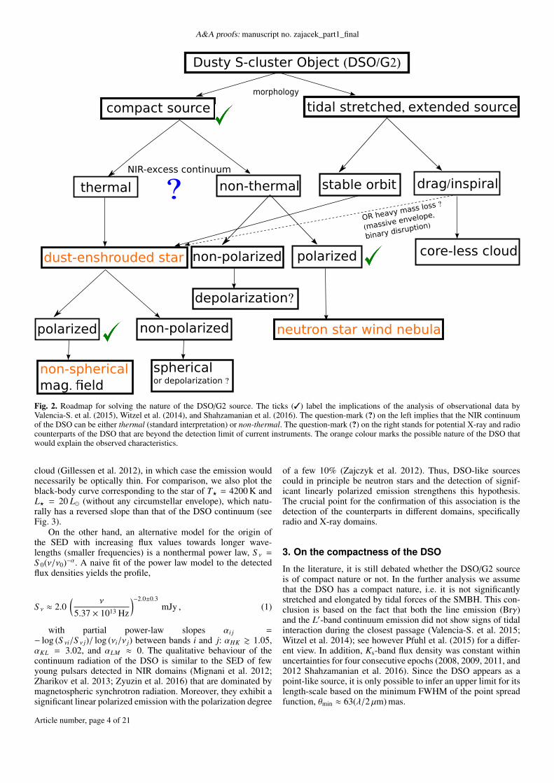
Since different aspects are involved, we set up the roadmaptowards solving the DSO nature, which is illustrated in Fig. 2.

In the further analysis, we consider the results of Valencia-S. et al. (2015) that show that the DSO exhibits a single-peakBrγ emission line at each epoch, i.e. they detect no significantstretching along the orbit as would be expected for a core-lesscloud. A consistent result is presented by Witzel et al. (2014),who detect a compact L-band emission of the DSO/G2 duringthe peribothron2 passage in 2014.

Therefore, we are not going to consider the tidal stretching,which according to the roadmap in Fig. 2 would either indicatean extended circumstellar envelope that does not feel the grav-itational field of the star, or a core-less cloud. These two sce-narios will be further tested by the orbital evolution in the post-peribothron phase.

Concerning the spectral energy distribution of the DSO, weadopt the results of Gillessen et al. (2012), Eckart et al. (2013),and Shahzamanian et al. (2016); see also Shcherbakov (2014)for the first SED analysis of the DSO assuming a core-less cloudscenario. As analysed by Eckart et al. (2013) and confirmed byShahzamanian et al. (2016), the source shows prominent redden-ing between NIR Ks and L′ bands, Ks−L′ > 3. Further measure-ments in M band were performed by Gillessen et al. (2012). TheH-band flux density is an upper limit since there was no detec-tion (Gillessen et al. 2012; Eckart et al. 2013).

In the NIR H band, Eckart et al. (2013) derive the mini-mum apparent magnitude of mH > 21.2 based on the backgroundlevel of the neighbouring stars. Using the extinction correction ofAH = 4.21, the upper limit on the flux density is FH . 0.17 mJy.

For the flux density in NIR Ks-band, we take a weighed meanof the measurements by Shahzamanian et al. (2016) (see our Ta-ble 3 for the summary of measurements). We obtain the meanflux density value of F2.2 = (0.23 ± 0.02) mJy, both with and2 We use pericentre and peribothron interchangeably; peribothron isderived from Greek bothros, which means a hole dug in the ground,also a pit used for drink offerings for subterranean gods in the Greekmythology.

without considering the epoch 2011, when the ratio S/N waslow.

For the L′-band magnitude, we consider the value of mL′ =14.4 ± 0.3 (Eckart et al. 2013). Using AL′ = 1.09, we obtain theflux density of F3.8 = (1.2 ± 0.3) mJy.

The absolute dereddened M-band magnitude obtained byGillessen et al. (2012) is MM = −1.8 ± 0.3, which yieldsF4.7 = (1.2 ± 0.4) mJy.

Table 2. Summary of NIR flux densities of the DSO. References:1) Eckart et al. (2013); 2) Eckart et al. (2013); Shahzamanian et al.(2016); 3) Gillessen et al. (2012); Eckart et al. (2013); Witzel et al.(2014); 4) Gillessen et al. (2012).

Band Wavelength [µm] Frequency [Hz] Flux density [mJy] Refs.H 1.65 1.82 × 1014 . 0.17 1)Ks 2.2 1.36 × 1014 0.23 ± 0.02 2)L′ 3.8 7.89 × 1013 1.2 ± 0.3 3)M 4.7 6.38 × 1013 1.2 ± 0.4 4)

The overall flux densities are summarized in Table 2. Basedon the flux density measurements, the upper limit on the overallluminosity was set to be LDSO < 30 L (Eckart et al. 2013; Witzelet al. 2014).

Another important constraint is the detection of polarizedemission in NIR Ks band by Shahzamanian et al. (2016) withthe polarization degree of ∼ 30% and a variable polarization an-gle for four consecutive epochs (2008, 2009, 2011, and 2012).The summary of all observational constraints is in Table 3.

Table 3. Summary of observational constraints for the DSO nature.

Constraint NoteSED "red" source; Ks − L′ > 3

broad emission lines FWHMBrγ ∼ 100 km s−1

source of polarized Ks band emission polarization degree ∼ 30%stability and compactness no significant tidal elongation

The dereddened, continuum flux densities in the NIR domainwere attributed to the warm dust emission in the temperature in-terval Tdust = 400 K–600 K (Gillessen et al. 2012; Eckart et al.2013), which can reproduce the flux densities between Ks andM bands. In Fig. 3, we repeat the fit of the dereddened fluxdensities with a single-temperature black-body flux density pro-file S ν(T,R) = (R/d)2πBν(T ), where Bν(T ) is a black-body spe-cific intensity at temperature T , R is the characteristic radius ofthe object, and d is the distance to the Galactic centre, whichwe set to d = 8 kpc (Eckart et al. 2005; Genzel et al. 2010;Eckart et al. 2017). The black-body fits gives the temperatureof T = (874 ± 54) K, which corresponds to the warm dust com-ponent, and the characteristic radius of R = (0.31± 0.07) AU foran optically thick black body. This corresponds to a rather com-pact source in comparison with the originally proposed meanlength-scale of Rc ≈ 15 mas ≈ 120 AU for a core-less gas



Dusty S-cluster Object (DSO/G2)

compact source tidal stretched, extended source

thermal non-thermal

NIR-excess continuum

morphology

dust-enshrouded star

polarized non-polarized

non-spherical

mag. eld

sphericalor depolarization ?

stable orbit drag/inspiral

core-less cloudnon-polarized polarized

neutron star wind nebula

depolarization?

OR heavy mass loss ?

(massive envelope,

binary disruption)

?

Fig. 2. Roadmap for solving the nature of the DSO/G2 source. The ticks (3) label the implications of the analysis of observational data byValencia-S. et al. (2015), Witzel et al. (2014), and Shahzamanian et al. (2016). The question-mark (?) on the left implies that the NIR continuumof the DSO can be either thermal (standard interpretation) or non-thermal. The question-mark (?) on the right stands for potential X-ray and radiocounterparts of the DSO that are beyond the detection limit of current instruments. The orange colour marks the possible nature of the DSO thatwould explain the observed characteristics.

cloud (Gillessen et al. 2012), in which case the emission wouldnecessarily be optically thin. For comparison, we also plot theblack-body curve corresponding to the star of T? = 4200 K andL? = 20 L (without any circumstellar envelope), which natu-rally has a reversed slope than that of the DSO continuum (seeFig. 3).

On the other hand, an alternative model for the origin ofthe SED with increasing flux values towards longer wave-lengths (smaller frequencies) is a nonthermal power law, S ν =S 0(ν/ν0)−α. A naive fit of the power law model to the detectedflux densities yields the profile,

S ν ≈ 2.0(

ν

5.37 × 1013 Hz

)−2.0±0.3mJy , (1)

with partial power-law slopes αi j =− log (S νi/S ν j)/ log (νi/ν j) between bands i and j: αHK & 1.05,αKL = 3.02, and αLM ≈ 0. The qualitative behaviour of thecontinuum radiation of the DSO is similar to the SED of fewyoung pulsars detected in NIR domains (Mignani et al. 2012;Zharikov et al. 2013; Zyuzin et al. 2016) that are dominated bymagnetospheric synchrotron radiation. Moreover, they exhibit asignificant linear polarized emission with the polarization degree

of a few 10% (Zajczyk et al. 2012). Thus, DSO-like sourcescould in principle be neutron stars and the detection of signif-icant linearly polarized emission strengthens this hypothesis.The crucial point for the confirmation of this association is thedetection of the counterparts in different domains, specificallyradio and X-ray domains.

3. On the compactness of the DSO

In the literature, it is still debated whether the DSO/G2 sourceis of compact nature or not. In the further analysis we assumethat the DSO has a compact nature, i.e. it is not significantlystretched and elongated by tidal forces of the SMBH. This con-clusion is based on the fact that both the line emission (Brγ)and the L′-band continuum emission did not show signs of tidalinteraction during the closest passage (Valencia-S. et al. 2015;Witzel et al. 2014); see however Pfuhl et al. (2015) for a differ-ent view. In addition, Ks-band flux density was constant withinuncertainties for four consecutive epochs (2008, 2009, 2011, and2012 Shahzamanian et al. 2016). Since the DSO appears as apoint-like source, it is only possible to infer an upper limit for itslength-scale based on the minimum FWHM of the point spreadfunction, θmin ≈ 63(λ/2 µm) mas.



100 101

λ [µm]

10-5

10-4

10-3

10-2

10-1

100

101

102

103

104

105

Fλ [m

Jy]

HKs

L′ M

star: T=4200K, L=20Lsun

blackbody fit: R=(0.31±0.07)AU, T=(874±54)K

nonthermal power-law fit: α=2.0±0.3

Fig. 3. Detected, dereddened flux densities of the DSO (black points)and the fitted continuum: thermal black-body fit curve corresponding towarm dust (orange solid and dashed lines) and nonthermal power-lawemission fit S ν ∝ ν

−α with the index α = 2.0± 0.3 (red solid and dashedlines). For comparison, we also plot the black-body curve correspond-ing to the star of T? = 4200 K and L? = 20 L (pre-main-sequence starwithout a dusty envelope; gray solid line).

A simple test of the compactness of the DSO is provided bythe comparison of the observed evolution with that of a core-lessgaseous stream approaching the black hole of M• = 4 × 106 M.When the parts of the cloud move independently in the potentialof the black hole, the cloud with initial radius Rinit is stretchedalong the orbit and compressed in the perpendicular direction.

According to Shcherbakov (2014), we can express the rela-tive prolongation as function of distance r from the SMBH interms of the half-length L,

Λ =L

Rinit=

( rinit

r

)1/2(

rA + rP − rrA + rP − rinit

)1/2

, (2)

where rinit is the initial distance at which the cloud was formed,having a spherical shape with the radius Rinit, and rP and rAare pericentre and apocentre distances of the DSO, respectively.We set rinit to the distance that corresponds to 10 years beforethe peribothron passage (earlier date of formation would lead tolarger prolongation). Similarly, the relative compression ρ in thedirection perpendicular to the orbit may be expressed as,

ρ = H/Rinit =r

rinit. (3)

where H is the actual perpendicular cross-section of the cloud.For the orbital parameters of the DSO (Valencia-S. et al. 2015),both the relative prolongation Λ(t) and compression ρ(t) are plot-ted in Fig. 4 (right panel) as functions of time before the peri-bothron passage. For the observed dimensions of the object, theforeshortening due to the orbital inclination is important. Theforeshortening factor as function of time is plotted in Fig. 4 (leftpanel). At the peribothron, the source should be viewed at fullsize and the relative prolongation is ∼ 6 times that of the ini-tial size (∼ 10 times when foreshortening is taken into account).The compression in the perpendicular direction should lead tothe general spaghettification of the cloud. The tidal elongation

of this order was, however, not detected (Witzel et al. 2014;Valencia-S. et al. 2015).

Specifically, between the epoch 2011.39 (3 years before theperibothron) and the peribothron passage, the prolongation fac-tor is Λ ' 3.45. If the DSO was a core-less cloud, it should havea pericentre length-scale Lper = ΛRinit. Gillessen et al. (2013b)infer the FWHM length-scale RFWHM = (42 ± 10) mas from theGaussian fit for epochs 2008.0, 2010.0, 2011.0, 2012.0, 2013.0.The pericentre size, with respect to 2011 epoch, should then beLper ≈ 145 mas > θmin, which is more than a factor of two largerthan PSF FWHM. Such a large size is inconsistent with a rathercompact line emission detected by Valencia-S. et al. (2015) dur-ing the pericentre passage. In fact, the analysis of the L-bandcontinuum emission of the DSO during the pericentre passageby Witzel et al. (2014) yields the diameter of 32 mas, i.e. fullyconsistent with a point source.

On the other hand, since the DSO was detected as a pointsource at the pericentre, the upper limit on its length-scale isgiven by the diffraction limit Lper ≤ θmin ≈ 63 mas. A core-lesscloud or an extended envelope of a star that reached the sizeof Lper by tidal stretching must have been smaller by a factorof Λ(−10 yr) ≈ 6, i.e. 10 years before the peribothron passage,yielding the characteristic size of L(−10 yr) . 10 mas ≈ 80 AU.Based on this estimate, we set the characteristic radius of thepotentially tidally perturbed part of the DSO to Rc . 5 mas.

Using the observationally inferred Brγ luminosity of LBrγ ≈

2 × 10−3 L (Gillessen et al. 2012; Valencia-S. et al. 2015), wecan estimate the electron density in the envelope assuming caseB recombination (Gillessen et al. 2012),

ne = 1.35 × 106 f −1/2V

( Rc

5 mas

)−3/2 (Tg

104 K

)0.54

cm−3 , (4)

where Tg is the expected gas temperature of the DSO and fV isthe volume filling factor, which we set to fV ≤ 1. For the massof the DSO, in case it would be a gas cloud, we get

MDSO,cloud ' 2.2 × 1027 f 1/2V

( Rc

5 mas

)3/2 (Tg

104 K

)0.54

g (5)

which is about MDSO,cloud = 0.4 f 1/2V MEarth. A smaller mass and

a required higher density than originally estimated (Gillessenet al. 2012) shorten typical hydrodynamical time-scales that de-termine the lifetime of the cloud, specifically the cloud evapora-tion time-scale is (Burkert et al. 2012)

τevap = 43( r5.4 × 1016

)1/6(

MDSO,cloud

2.2 × 1027 g

)1/3

yr , (6)

where r is the distance from Sgr A* in units of 5.4 × 1016 cm,which corresponds approx. to the epoch of 2004. Such a shortevaporation time-scale for a small, cold clump in the hot ambi-ent plasma would necessarily lead to observable changes in thecloud line and continuum luminosities. However, the observa-tions imply that the DSO is a rather compact, stable source inboth line and continuum emission (Witzel et al. 2014; Valencia-S. et al. 2015; Shahzamanian et al. 2016).

Although a magnetically arrested cloud was suggested to ex-plain the apparent stability (Shcherbakov 2014), it would stillnot prevent the cloud from the progressive evaporation and dis-ruption (McCourt et al. 2015) as well as the loss of angular mo-mentum when interacting with the ambient medium, leading tothe inspiral and deviation from the original ellipse (Pfuhl et al.2015; McCourt et al. 2015).



Therefore, given the reasons above, a stellar nature of theDSO is more consistent with its observed line and continuumcharacteristics.

The basic estimate of the distance rt where an object with acharacteristic radius RDSO and mass MDSO is tidally disruptedis given by rt = RDSO(3M•/MDSO)1/3. For a stellar source,we get an estimate rt ' 1.07(RDSO/1R)(MDSO/1M)−1/3 AU.Since the peribothron distance of the DSO is rP = a(1 − e) =0.033 pc × (1 − 0.976) ≈ 163 AU (Valencia-S. et al. 2015) andno visible tidal interaction was observed, the upper limit on thelength-scale of the stellar system that stays stable is RDSO ≈

0.7 (MDSO/1 M)1/3 AU. On the other hand, for the cloud ofRDSO = 15 mas ≈ 2.7 × 104 R and the mass of three Earthmass, MDSO ≈ 10−5 M (Gillessen et al. 2012), the tidal radius isrt ≈ 1.3×106 AU. Hence, the cloud should be strongly perturbednot only at the pericentre, but during the whole phase of infall,since the apocentre distance is rA = a(1 + e) ≈ 1.3 × 104 AU.In summary, to explain the compact behaviour of the object, theemitting material (gas+dust) should be located in the inner as-tronomical unit from the star.

On the other hand, since the NIR-continuum is dominatedby thermal dust emission (for a dust-enshrouded star), one canestimate the lower distance limit where the dust is located fromthe dust sublimation radius rsub (Monnier & Millan-Gabet 2002),

rsub = 1.1√

QR

(LDSO

1000 L

)1/2 ( Tsub

1500 K

)−2

AU , (7)

where QR is the ratio of absorption efficiencies, which we con-sider to be of the order of unity, and Tsub is the dust sublimationtemperature, for which we take 1500 K. The inferred luminosityof the DSO is of the order of LDSO ≈ 10 L (Eckart et al. 2013;Witzel et al. 2014), and so the expected sublimation radius isrsub ≈ 0.1 AU. Hence, since the continuum emission seems to becompact and no clear evidence of tidal interaction was detectedduring the peribothron passage (Witzel et al. 2014), the distancerange, where the dust emitting the NIR-continuum is located andstays gravitationally unperturbed, is quite narrow, rsub . r . rt,i.e. 0.1 AU . r . 1 AU.

4. Modelling the total and polarized continuumemission of the DSO

In this section, we focus on the modelling of the total as well aspolarized flux density in corresponding NIR bands.

The main aim is the continuum radiative transfer in the densedusty envelope surrounding a star with the emphasis on the lin-early polarized emission (Section 4.1). The continuum profileis shaped by reprocessing the stellar emission by the surround-ing dusty envelope. Linear polarization may arise due to (i)photon scattering on spherical dust grains (Mie scattering), (ii)dichroic extinction caused by selective absorption of photons inthe medium where non-spherical grains are aligned due to radia-tion or magnetic field. The overall linear polarization degree foryoung stars may vary from the fraction of a percent up to a few10%, depending on the geometry as well as the extinction of thedusty envelope (see Kolokolova et al. 2015, for a review).

In case of a hypothetical non-thermal origin of the DSO con-tinuum (Section 4.2, one expects a slope of the flux densityS ν ∝ ν−n, where n > 0. Typically, young neutron stars exhibita multiwavelength non-thermal continuum, which arises due tothe synchrotron process in the magnetosphere of young neutron

stars. Another contribution is the thermal emission of the cool-ing surface. However, for young (. 10 kyr) and middle-aged(& 100 kyr) neutron stars, the non-thermal component dominatesin NIR bands. Since neutron stars typically possess a highly-ordered strong magnetic field, the non-thermal component isexpected to be partially linearly polarized. Using the homoge-neous magnetic field approximation, the linear polarization de-gree for the synchrotron emission can be determined as (Rybicki& Lightman 1979),

PL .n + 1

n + 5/3, (8)

where for n ≈ 0.7 one gets PL . 0.72, whereas the measuredvalue in Ks band (VLT/ISAAC) is Pavg

L ' 0.47 (Zajczyk et al.2012) for the surrounding pulsar wind nebula.

4.1. Thermal origin of the SED: DSO as a dust-enshroudedstar

To find the model of a dust-enshrouded star that reproduces theobserved characteristics (SED, broad emission lines, linear po-larization, and overall stability and compactness; see also Table 3for the summary) we perform a set of 3D dust continuum ra-diative transfer simulations with different components and mor-phologies of dusty envelopes.

For solving the radiative transfer equation, we choose aMonte Carlo technique suitable for arbitrary three-dimensionaldusty envelopes (Whitney 2011). For all our simulations of adust-enshrouded star, we used an open-source parallelized codeHyperion (Robitaille 2011), which enables to create SEDs aswell as images for a required wavelength range as well as dif-ferent inclinations of the source. Since in the random walk ofphotons the scattering process is also included, we obtain a fullStokes vector (I,Q,U,V), which enables us to calculate the lin-ear polarization degree as well as the angle according to standarddefinitions,

PL =

√Q2 + U2

I,

φ =12

arctan(

UQ

). (9)

Since the extinction is expected to be high in the innermostparts of the envelope, we make use of a modified random walk(MRW) implemented in the code in the thickest regions.

An important part of the modelling is the generation of thedust distribution, for which we use the code bhmie by C.F.Bohren and D. Huffman (improved by B. Draine; Bohren et al.,1998), which provides solutions to the Mie scattering and ab-sorption of light by spherical dust particles. We generate dustgrains with a power-law distribution n(a) ∝ a−3.5 with the small-est and the largest grain size of (amin, amax) = (0.01, 10.0) µm.The gas-to-dust mass ratio in the dusty circumstellar envelopefor all geometries is assumed to be 100. The distance to theGalactic centre is set to 8 kpc for flux density calculations.

For most of the simulations, we set up a 3D spherical gridthat contains 400 × 200 × 10 grid points, and add a density gridof gaseous-dusty mixture with the dust properties as explainedabove.

For all synthetic SEDs and images, the total flux density wasdetermined via the integration over the whole source and thencompared to observationally determined values in Table 2.



0.3

0.4

0.5

0.6

0.7

0.8

0.9

1

-10 -5 0 5 10

fore

short

enin

g facto

r

(t-t0) [yr]

0.01

0.1

1

10

100

-10 -8 -6 -4 -2 0

rela

tive p

rolo

ngation a

nd c

om

pre

ssio

n (

gaseous s

tream

)

(t-t0) [yr]

relative prolongation along the orbitprojected relative prolongation

relative compression along the orbitprojected relative compression

Fig. 4. Left: Foreshortening factor for the size of any structure calculated for the DSO orbit with inclination i = 113. Right: Relative tidalstretching and compression as function of time (in years with respect to the peribothron passage) in the orbital plane (solid lines) and with respectto the inclined orbit to the DSO.

4.1.1. Different morphologies: source components

At first, we performed radiative transfer calculations for differentgeometries of circumstellar envelopes to assess whether they canreproduce the detected high polarization degree in Ks-band andthe NIR-excess. First, we started with the simplest models with astar at the centre and flattened envelope and/or bow shock. For allthese cases, the polarization degree remains below 10%. Break-ing the spherical symmetry by introducing the cavities, havinghalf-opening angle of 45, increases the polarization degree to∼ 10% (without a bow shock layer). Adding a dense bow shocklayer, the linear polarization fraction typically reaches > 20%,depending on the density of the envelope and the inclination.Qualitatively, the dependence of the linear polarization degreeon the envelope geometry is sketched in Figure 9.

The density grid in the radiative transfer models has differ-ent morphological and density components, whose characteris-tics are explained below:

– star: Based on the upper luminosity limit of LDSO . 30 L(Eckart et al. 2013; Witzel et al. 2014), the central star of theDSO should belong to the category of pre-main-sequencestars with the mass constraint M? . 3M (Zajacek et al.2015). Given the NIR-excess, i.e. the rising SED longwardof 2 microns, it should belong to the category of class Iobjects – protostars (Lada 1987)3 with an age of 105 yr upto 106 yr. The comparison of stellar evolutionary tracks fordifferent masses is in Fig. 5 for the metallicity fraction ofZ = 0.02, which was constructed based on the computedtables by Siess et al. (2000). In the set of Monte Carlo sim-ulations, we vary the luminosity and the temperature of starsto fit the observed flux density values and we get reasonablematch for M? = 1.3 M, L? = 19.6 L and Teff = 4220 K– labelled as the red cross in Fig. 5. These stellar parame-ters were used in all the simulations presented in this paper,unless indicated otherwise.

– flattened envelope: To the first approximation, the dust-enshrouded star may be modelled as a star surrounded bya rotationally flattened, infalling dusty envelope that forms a

3 The Lada-Wilking morphological classification of young stel-lar objects based on the spectral slope of their SEDs, α =d log (λFλ)/d log (λ): class I sources (0 < α . 3), class II sources(−2 . α ≤ 0), and class III sources (−3 < α . −2).

-1.5

-1

-0.5

0

0.5

1

1.5

2

2.5

3

3.5

3.5 3.6 3.7 3.8 3.9 4 4.1

log(L/L

Sun)

log[Teff]K

DSO/G2

R/Rsun=1

R/Rsun=10

105 yr

106 yr

107 yr

0.5 Msun1.0 Msun1.3 Msun1.5 Msun2.0 Msun2.5 Msun3.0 Msun3.5 Msun

Fig. 5. A set of the evolutionary tracks of pre-main-sequence stars basedon Siess et al. (2000). The red line marks the upper limit for the bolo-metric luminosity of the DSO, LDSO . 30 L. The orange solid linedepicts the mass of 1.3 M, which we used for choosing the input pa-rameters for radiative transfer calculations (red point).

disc at the corotation radius rc. The density profile is givenby (Ulrich 1976),

ρ(r, θ) =Macc

4π(GMDSOr3c )1/2

(rrc

)−3/2 (1 +

µ

µ0

)−1/2

×

µµ0

+2µ2

0rc

r

−1

, (10)

where Macc is the infall rate. The quantities µ and µ0 are re-lated by an equation of the streamline, µ3

0 + µ0(r/rc − 1) −µ(r/rc) = 0.The model of Ulrich envelope can match the SED of theDSO for stellar parameters M? = 1.3 M, L? = 4.3 L,Teff = 4400 K, R? = 3.3 R (age ∼ 760 000 yr). The suit-able parameters of the envelope are Macc = 5×10−7 M yr−1,rmin = 10 R?, and rc = 20 R?, where rmin is the mini-mal distance of the envelope from the star. We vary themaximum distance of the envelope rmax from 0.5 AU up to



1 2 3 4 5 6 7 8 9 10λ [µm]

10-1

100

101

Fλ [m

Jy]

H Ks L′ M

rmax=0.5AU

0 30 60 90

1 2 3 4 5 6 7 8 9 10λ [µm]

10-1

100

101

Fλ [m

Jy]

H Ks L′ M

rmax=5AU

0 30 60 90

1 2 3 4 5 6 7 8 9 10λ [µm]

10-1

100

101

Fλ [m

Jy]

H Ks L′ M

rmax=50AU

0 30 60 90

Fig. 6. Model SEDs of a star surrounded by rotationally flattened envelope for different inclinations in the range (0, 90) with an increment of30, see the key for different linestyles representing different inclinations. The points with error bars correspond to observationally inferred values,see Table 2. Left panel: The maximum radius of the envelope is set to rmax = 0.5 AU. Middle panel: rmax = 5 AU. Right panel: rmax = 50 AU.

1 2 3 4 5 6 7 8 9 10λ [µm]

10-1

100

101

Fλ [m

Jy]

H Ks L′ M

Macc=5×10−6Msunyr−1

0 30 60 90

1 2 3 4 5 6 7 8 9 10λ [µm]

10-1

100

101

Fλ [m

Jy]

H Ks L′ M


0 30 60 90

1 2 3 4 5 6 7 8 9 10λ [µm]

10-1

100

101

Fλ [m

Jy]

H Ks L′ M


0 30 60 90

Fig. 7. Model SEDs of a star surrounded by rotationally flattened envelope with the fixed maximum radius of rmax = 5 AU for different inclinationsin the range (0, 90) with an increment of 30, see the key for different linestyles representing different inclinations. The points with error barscorrespond to observationally inferred values, see Table 2. Left panel: The accretion rate is set to Macc = 5 × 10−6 Myr−1. Middle panel:Macc = 5 × 10−7 Myr−1. Right panel: Macc = 5 × 10−8 Myr−1.

50 AU, which affects the SED due to a different dust tem-perature distribution. For the SEDs of the flattened envelopeat different inclinations (0, 30, 60, 90) and three differ-ent maximum radii rmax = [0.5, 5, 50] AU, see Fig. 6. Be-cause of observational uncertainties, more suitable config-urations are possible, e.g. rmax = 5 AU and the inclinationof 90 or rmax = 50 AU and the inclination in the range ofi = (60, 90). The lower value of rmax = 0.5 AU is not suit-able because of the large flux in Ks band, which can be ex-plained by a lower extinction and a more prominent stellaremission. In the range rmax = (5, 50) AU, the SED does notdepend much on this parameter because of the decreasing gasand dust density according to Eq. (10). On the other hand, theSED depends strongly on the accretion rate Macc. We varythe accretion rate between Macc = (5×10−6, 5×10−8) M yr−1

for the fixed maximum radius of rmax = 5 AU, see Fig. 7.Clearly, the best match of SED values is for an intermediatevalue of Macc = 5 × 10−7 M yr−1 (Middle panel), increas-ing or decreasing the accretion rate by an order of magnitudesignificantly changes calculated fluxes, which is caused bylarge changes in the dust density, ρ ∝ Macc, see Eq. (10). Al-though a star surrounded by a flattened envelope can satisfac-torily explain the SED of the DSO, the calculated polarizedemission in Ks band from radiative transfer models yieldsthe maximum total polarization degree of pK,L = 2.7% fori = 90, i.e. well below the detected value of ∼ 30% (Shahza-manian et al. 2016). This implies that the simple geometry ofthe flattened envelope cannot alone explain the properties ofthe DSO.

– spherically concentrated dusty envelope/flared disc: Formore complex models, we set up a stratified spherical dustyenvelope that was intersected by bipolar cavities in somemodels with smaller number densities (see below). In the fi-nal set of models, the spectral slope could be reproduced bythe following mean mass densities of the gas+dust mixture:1×10−13 g cm−3 for r = 0.1 AU–1.0 AU, 1×10−14 g cm−3 forr = 1.0 AU–2.0 AU, and 1 × 10−15 g cm−3 for r = 2.0 AU–3.0 AU.

– bipolar cavity: The bipolar cavities were introduced in themodel to increase the non-spherical nature of the DSO,which is naturally needed to obtain a non-zero total polariza-tion degree in the model, see Fig. 9. Furthermore, the wallsof cavities also provide effective space for single scatteringevents of stellar and dust photons that escape from the starand the envelope, respectively. The density inside cavities isset to be uniform and smaller than in the envelope by severalorders of magnitude: 1 × 10−20 g cm−3, which is a typical or-der of magnitude (see e.g. Sanchez-Bermudez et al. 2016).The half-opening angle of the cavity is initially varied to in-vestigate the impact of the parameter space on the SED andthe polarization, then set to θ0 = 45.

– bow shock: The DSO and other objects in the S-clusterare expected to move supersonically through the ambientmedium, especially close to the pericentre of their orbits (seeFig. 1 in Zajacek et al. 2016), see also De Colle et al. (2014);Ballone et al. (2013, 2016); Christie et al. (2016). The ex-pected Mach number of the DSO is M = vrel/cs . 10 (Za-jacek et al. 2016), where vrel is the relative velocity of theDSO with respect to the medium and cs is the local sound



102

103

104

105

106

107

108

109

1010

-10 -8 -6 -4 -2 0

bow

-shock n

um

ber

density [cm

-3]

(t-t0) [yrs]

2008

2009

2011

2012

10 km s-1

100 km s-1

1000 km s-1

1

1.5

2

2.5

3

3.5

4

4.5

5

-6 -5.5 -5 -4.5 -4 -3.5 -3 -2.5

bow

-shock d

ensity c

hange (

2008-2

012)

(t-t0) [yrs]

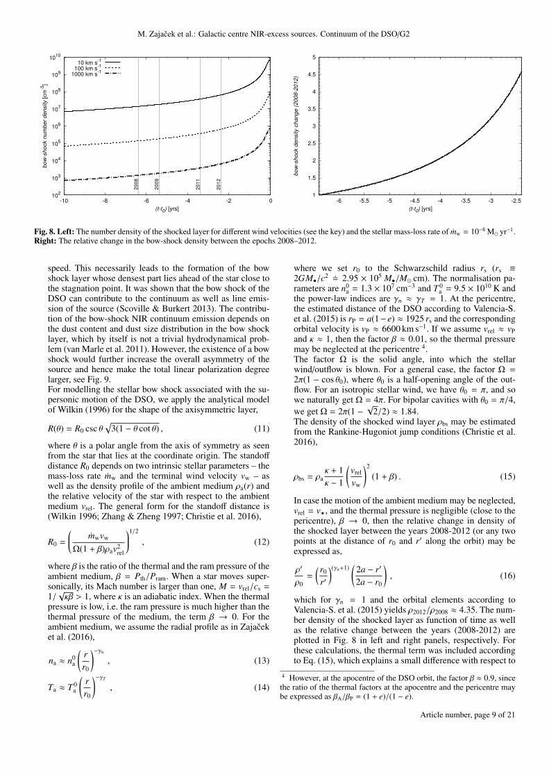
Fig. 8. Left: The number density of the shocked layer for different wind velocities (see the key) and the stellar mass-loss rate of mw = 10−8 M yr−1.Right: The relative change in the bow-shock density between the epochs 2008–2012.

speed. This necessarily leads to the formation of the bowshock layer whose densest part lies ahead of the star close tothe stagnation point. It was shown that the bow shock of theDSO can contribute to the continuum as well as line emis-sion of the source (Scoville & Burkert 2013). The contribu-tion of the bow-shock NIR continuum emission depends onthe dust content and dust size distribution in the bow shocklayer, which by itself is not a trivial hydrodynamical prob-lem (van Marle et al. 2011). However, the existence of a bowshock would further increase the overall asymmetry of thesource and hence make the total linear polarization degreelarger, see Fig. 9.For modelling the stellar bow shock associated with the su-personic motion of the DSO, we apply the analytical modelof Wilkin (1996) for the shape of the axisymmetric layer,

R(θ) = R0 csc θ√

3(1 − θ cot θ) , (11)

where θ is a polar angle from the axis of symmetry as seenfrom the star that lies at the coordinate origin. The standoffdistance R0 depends on two intrinsic stellar parameters – themass-loss rate mw and the terminal wind velocity vw – aswell as the density profile of the ambient medium ρa(r) andthe relative velocity of the star with respect to the ambientmedium vrel. The general form for the standoff distance is(Wilkin 1996; Zhang & Zheng 1997; Christie et al. 2016),

R0 =

mwvw

Ω(1 + β)ρav2rel

1/2

, (12)

where β is the ratio of the thermal and the ram pressure of theambient medium, β = Pth/Pram. When a star moves super-sonically, its Mach number is larger than one, M = vrel/cs =1/√κβ > 1, where κ is an adiabatic index. When the thermal

pressure is low, i.e. the ram pressure is much higher than thethermal pressure of the medium, the term β → 0. For theambient medium, we assume the radial profile as in Zajaceket al. (2016),

na ≈ n0a

(rr0

)−γn

, (13)

Ta ≈ T 0a

(rr0

)−γT

, (14)

where we set r0 to the Schwarzschild radius rs (rs ≡

2GM•/c2 2.95 × 105 M•/M cm). The normalisation pa-rameters are n0

a = 1.3 × 107 cm−3 and T 0a = 9.5 × 1010 K and

the power-law indices are γn ≈ γT = 1. At the pericentre,the estimated distance of the DSO according to Valencia-S.et al. (2015) is rP = a(1− e) ≈ 1925 rs and the correspondingorbital velocity is vP ≈ 6600 km s−1. If we assume vrel ≈ vPand κ ≈ 1, then the factor β ≈ 0.01, so the thermal pressuremay be neglected at the pericentre 4.The factor Ω is the solid angle, into which the stellarwind/outflow is blown. For a general case, the factor Ω =2π(1 − cos θ0), where θ0 is a half-opening angle of the out-flow. For an isotropic stellar wind, we have θ0 = π, and sowe naturally get Ω = 4π. For bipolar cavities with θ0 = π/4,we get Ω = 2π(1 −

√2/2) ≈ 1.84.

The density of the shocked wind layer ρbs may be estimatedfrom the Rankine-Hugoniot jump conditions (Christie et al.2016),

ρbs = ρaκ + 1κ − 1

(vrel

vw

)2

(1 + β) . (15)

In case the motion of the ambient medium may be neglected,vrel = v?, and the thermal pressure is negligible (close to thepericentre), β → 0, then the relative change in density ofthe shocked layer between the years 2008-2012 (or any twopoints at the distance of r0 and r′ along the orbit) may beexpressed as,

ρ′

ρ0=

( r0

r′

)(γn+1)(

2a − r′

2a − r0

), (16)

which for γn = 1 and the orbital elements according toValencia-S. et al. (2015) yields ρ2012/ρ2008 ≈ 4.35. The num-ber density of the shocked layer as function of time as wellas the relative change between the years (2008-2012) areplotted in Fig. 8 in left and right panels, respectively. Forthese calculations, the thermal term was included accordingto Eq. (15), which explains a small difference with respect to

4 However, at the apocentre of the DSO orbit, the factor β ≈ 0.9, sincethe ratio of the thermal factors at the apocentre and the pericentre maybe expressed as βA/βP = (1 + e)/(1 − e).



the estimate of the relative density increase above. The stellarparameters were adopted from the previous analysis of Scov-ille & Burkert (2013) and Zajacek et al. (2016): the mass-lossrate mw = 10−8 M yr−1 and variable wind velocities in therange 10 km s−1–1000 km s−1. For the radiative transfer sim-ulations, we tried different values of the bow-shock densityand the best match to the observed SED and the polarizedemission was reached for vw = 10 km s−1, i.e. slow outflow.

The summary of the polarization degree and the sourcecolour (Ks−L′) (with and without line-of-sight extinction) for allthe circumstellar geometries, which were tested, is summarizedin Table 4.

4.1.2. Final model: supersonic, dust-enshrouded star withnon-spherical envelope

Star

+

spherical dusty envelope

Star

+

dusty envelope

+

bipolar cavities

Star

+

dusty envelope

+

bipolar cavities

+

bow shock

breaking the spherical symmetry

increasing the total linear polarization degree

Plinear(2.2 m): ~0% ~1-10% ~20-30%

Fig. 9. Sketch of how the geometry of circumstellar envelope affects thetotal linear polarization degree in Ks band.

From the set of radiative transfer simulations with differentcircumstellar geometries (see Table 4), the model that can meetall constraints listed in Table 3 consists of the following compo-nents:

– a pre-main-sequence star,– spherically concentrated dusty envelope/geometrically thick

disc,– bipolar cavity with a half-opening angle θ0 = 45,– bow shock,

The detailed discussion of the adopted parameters and densitiesof the gas/dust envelope is in the previous subsection. The il-lustration of the model is in Fig. 10 (left panel). An importantparameter in terms of the intrinsic geometry is the angle δ thatdetermines the orientation of the bipolar outflow with respect tothe axis of symmetry of the bow shock. Unless otherwise indi-cated, we set δ = 0, i.e. the bipolar cavities are aligned with thesymmetry axis of the bow shock.

An exemplary model SED is in Fig. 10 (right panel) calcu-lated for the viewing angle of 90. Here we use the same conven-tion for the viewing angle as Mužic et al., 2010, see their Fig.3 – 0 corresponds to the front view of the bow shock (circu-lar shape in projection), 90 corresponds to the side view (bow-shock shape), and 180 corresponds to the view from the tailpart (also circular shape in projection). The thick black solidline represents the total continuum flux density and thinner, graylines stand for individual components: stellar emission, scattered

stellar emission, dust emission, and scattered dust emission. It isclearly visible that L′-band flux density is dominated by the ther-mal dust emission (direct photons), whereas Ks-band emissionis dominated by scattered emission, mainly scattered dust pho-tons and to a smaller extent, scattered stellar photons. The stellarphotospheric emission is negligible across the whole NIR- andMIR-spectrum.

We also check the dependence of the SED on the viewing an-gle, see Fig. 11 (left panel). Quantitatively, the best match is forviewing angles larger than 50 and less than 130. The depen-dence of the SED on the viewing angle implies a possible sourceof continuum variability as the DSO source orbits Sgr A*. For Ksand L′ bands, the variability is a few 0.1 mJy within an expectedviewing angle ∼ 80–150, see Appendix A for estimates, whichdepend mainly on the relative velocity of the star with respectto the medium, which is in general uncertain. However, close tothe pericentre, the relative velocity should approach the orbitalvelocity.

The linear polarization degree as function of wavelength isdepicted in Fig. 11 (right panel). The largest total polarizationdegree, PL & 20%, is for the viewing angles close to 90 whenthe source is highly non-spherical. On the other hand, for theviewing angle either close to 0 or 180, the total linear polariza-tion degree is . 10%, since the source appears rather circular.

The dependence of the total linear polarization degree in Ksband on the inclination is in Fig 12 (right panel). For radiativetransfer calculations, we set the position angle of the bipolar cav-ities to δ = 0, i.e. aligned with the symmetry axis of the bowshock. The plot in Fig. 12 shows that a gradual increase in thebow-shock density (see also Fig. 8) over the interval 2008–2012leads to an increase in the total linear polarization degree overcertain inclination ranges. A potential increase in the polariza-tion degree is also discussed in Shahzamanian et al. (2016). It is,however, detected only for one epoch, 2012.0 (see their Fig. 4and Table 3), when the polarization degree reaches pL ' 37.6%,so a progressive increase cannot be considered significant at thispoint. In addition, Figure 12 implies that the polarization de-gree can change when the inclination of the source geometry(bow shock), i.e. the viewing angle with respect to the observer,changes for different epochs. Indeed, this is the case for the DSOdue to its fast motion along the elliptical orbit around Sgr A*,see also the calculation of the viewing angle variation close tothe pericentre passage presented in Appendix A. Furthermore,we perform the simulations for a bipolar outflow that is mis-aligned with the bow-shock symmetry axis. In Fig. 12, two ad-ditional dependencies for δ = 45 and δ = 90 are calculatedfor the largest density (epoch 2012.0). Given our model set-upand an expected range of viewing angles (see the shaded areain Fig. 12), the polarization degree of ∼ 30% is better repro-duced by the configuration, in which the position angle δ of thebipolar outflow is between 0–45, i.e. more aligned towards thebow-shock symmetry axis. When the orientation of the bipolaroutflow is perpendicular to the symmetry axis, δ = 90, the de-pendence of the polarization degree on the inclination is ratherflat and stays below or around 20%.

Qualitatively, all the polarization curves in Fig. 11 (rightpanel) have a peak that is close to 2.2 µm for the view-ing angles around 90, and the peak shifts towards shorterwavelengths for both smaller and larger viewing angles than90. The curves resemble the empirical Serkowski law, pL =pmax exp −K ln2 (λmax/λ) (Kolokolova et al. 2015), where λmaxis the wavelength at which the polarization curve reaches themaximum pL = pmax and the coefficient K determines the widthof the curve. However, the Serkowski law is used to fit the linear



Geometry Ks-band Total Linear Polarization Degree pK,L [%] (Ks − L′)int (intrinsic) (Ks − L′)ext = (Ks − L′)int + (AK − AL) (with extinction)Star 0 (∼ 6% foreground pol. at Gal. Ctr.) −0.9 0.4

Star+rotationally flattened envelope (90 inclination) 2.7 1.6 2.9Star+flared disc 3.2 0.3 1.6

Star+dense bow shock (inclined) 4.1 1.9 3.2Star+spherical dusty envelope+dense bow shock (inclined) 1.0 1.6 2.9

Star+flattened envelope+cavities (90% inclination) 10.1 1.2 2.4Star+flared disc+flattened envelope+cavities (90% inclination) 10.5 −1.3 −0.03

Star+envelope+cavities+dense bow shock 23.0 1.6 2.9Observations (Shahzamanian et al. 2016) ∼ 30 1.8 3.1

Table 4. Circumstellar geometries with a different set of components. Important parameters are the total linear polarization degree in Ks band(2.2 µm) and the colour index Ks − L′ (with and without line-of-sight extinction). The observed values for the polarization degree and thecolour index are also included. The observed values of the polarization degree and the colour index are matched best by the composite modelstar+disc+cavities+dense bow shock.

ow shock

DSO stellar model - components

Sgr A*rpambient plasma

Changes along the orbit- increase in bow shock density

- change of internal configuration

(disk precession - bipolar outflow)

- interaction with ambient medium

- change of the star-envelope

viewing angle

ou

disk wobbling/precession

1 2 3 4 5 6 7 8 9 10λ [µm]

10-5

10-4

10-3

10-2

10-1

100

101

102

103

104

Fλ [m

Jy]

HKs

L′ M

total flux densitystellar emissionscattered stellar emissiondust emissionscattered dust emission

Fig. 10. Left: Illustration of the components of the DSO model explained as a pre-main-sequence star. The right side explains possible sources ofthe changes in the continuum emission of the DSO/G2 (polarization degree and angle). Right: The calculated SED for the composite model of theDSO (star, dusty envelope, bipolar cavities, bow shock) for the viewing angle of 90. The thick solid line stands for the total continuum flux density,whereas gray lines represent individual source contributions (see the key). The points represent observationally inferred flux densities/limits forH, Ks, L′, and M bands.

polarization degree in the ISM that arises due to dichroic extinc-tion, whereas the simulations presented here are performed forspherical grains, and without the implementation of the magneticfield, whose configuration at the studied distances from Sgr A*is still highly uncertain and beyond the scope of this paper.

The variation of the position angle δ of the bipolar cavityleads to the change of the brightness distribution in the total aswell as the linearly polarized light, and hence the change of thepolarization angle Φ. In Shahzamanian et al. (2016) we fitted thedependency of the polarization angle on the position angle withthe relation that is approximately equal to Φ ≈ −(+)δ + (−)90(see Fig. 9 in Shahzamanian et al., 2016). This relation is alsoevident in the simulated images of the linear polarized light inFig. 13, where we change the position angle in 45 steps from0 up to 90 (from the top to the bottom panels in Fig. 13). Mostof the scattered, polarized light comes from the region where thebipolar cavities intersect the bow-shock shell. On the other hand,the minimum of the polarized emission is overlapping naturallywith the optically thick dusty envelope that also hides the star atthe centre.

Shahzamanian et al. (2016) measured a variable polarizationangle for four epochs, see their Fig. 4 (right panel). There are twopossible mechanisms that can be employed to explain a variablepolarization angle – see also the left panel of Fig. 10 for theillustration:

(i) intrinsic changes in the star-envelope orientation: thesechanges would be due to the torques induced by the massiveblack hole, which would lead to the precession of the circum-stellar disc/bipolar outflows in case the disc is misalignedwith respect to the orbital plane. The precession time-scale islonger than the orbital time-scale, Tprec > Torb. On the otherhand, the wobbling of the disc takes place on the time-scaleshorter than one orbital period, approx. Twobble ≈ 1/2Torb(Bate et al. 2000),

(ii) external interaction of the star with the nuclear out-flow/inflow: such an interaction could change the viewing an-gle on the star-bow shock-bipolar outflow system, especiallyfor the case when the outflow/inflow velocity is comparableto the orbital velocity of the star, which would significantlyaffect the relative velocity, vrel = vstar − va, and hence alsothe orientation of the bow shock with respect to the observer,see the modelling by Zajacek et al. (2016).

The simulated RGB image (Red colour - L′ band, Greencolour - M band, Blue colour - Ks band) of the source model ofthe DSO is in Fig. 14 with the labels of the components. For thesimulated image, we set the position angle δ to 90, i.e. perpen-dicular to the symmetry axis of the bow shock (compare with thesimulated image in Fig. 11 in Shahzamanian et al., 2016, whichwas computed for δ = 0.) The inset in Fig. 14 illustrates themagnetospheric accretion that was used to explain the origin of



1 2 3 4 5 6 7 8 9 10λ [µm]

10-2

10-1

100

101

102

Fλ [m

Jy]

H

Ks

L′M

02040

6080

100120

140160

1 2 3 4 5λ [µm]

0

10

20

30

40

linea

r polarization de

gree

[%]

02040

6080

100120

140160

Fig. 11. Left: The spectral energy distribution of the composite stellar model of the DSO as function of the viewing angle. The points representobservationally inferred values. Different viewing angles from 0 up to 180 are labelled by different colours according to the key. Right: Thelinear polarization degree as function of wavelength for different viewing angles (see the key). The vertical thick line marks the values along theKs band (2.2 µm), the horizontal line denotes the value of pL = 30%, which is close to observationally inferred values for four consecutive epochs(2008, 2009, 2011, 2012; Shahzamanian et al., 2016).

-120

-100

-80

-60

-40

-20

0

20

-100-50 0 50 100 150 200 250

∆DEC

[m

as]

∆RA [mas]

vw=100 km s-1

, va=0 km s-1

103

104

na [

cm

-3]

2008.0

2009.0

2011.0

2012.0Sgr A*

0

10

20

30

40

50

60

70

0 20 40 60 80 100 120 140 160 180

pL (

2.2

µm

) [d

egre

es]

inclination [degrees]

DSO viewing angle (2004.39-2014.39)

initial epoch (2008.0); δ=0o

epoch (2009.0): 1.3-times denser bow shock; δ=0o





Fig. 12. Left: Schematic plot of the bow-shock evolution of the DSO along the orbit. The mass-loss rate was taken to be mw = 10−8 M yr−1

and the terminal wind velocity is vw = 100 km s−1. The ambient density was colour-coded according the distribution expressed by Eq. 13. Right:Total linear polarization degree in Ks band for different inclinations (0–180 degrees) of the DSO composite model. According to the key, the solidlines represent different epochs, 2008–2012, with a gradually increasing bow-shock density (see also Fig. 8). The three orange lines associatedwith the largest bow-shock density represent the set-ups for three different position angles of the bipolar outflow, δ = 0, 45, and 90. Theshaded rectangular region represents different angles of the bow-shock axis with respect to the line of sight for the period of 10 years before thepericentre passage of the DSO, assuming a negligible motion of the ambient medium in comparison with the orbital velocity of the DSO. Thehorizontal dashed line marks the polarization degree value of pL = 30%, which is approximately the observationally inferred degree for the DSO(Shahzamanian et al. 2016).

the broad Brγ line of the DSO (Valencia-S. et al. 2015; Zajaceket al. 2015).

Independently of the previous analysis, where the Ks-bandflux density is linearly polarized mainly due to dust photons scat-tering off spherical dust grains, a correlation was found betweenthe linear polarization degree in Ks towards luminous stars em-bedded in molecular clouds and the optical depth τK, which canbe fitted by a power law (Kolokolova et al. 2015),

PL,K = 2.2τ0.75K (%) . (17)

Jones et al. (1992) explain this correlation by a 50/50 mixture ofthe constant, i.e. perfectly aligned, component to the magneticfield with random components.

When applied to the DSO with PDSO ' 30%, we get τDSO ≈

33 as an estimate for the optical depth to the object along the lineof sight, most of which can be attributed to the locally dense, op-tically thick envelope surrounding the stellar core. Similar valuesfor the polarization degree and the optical depth in Ks band werefound for the Becklin-Neugebauer object and OMC1-25 in theOrion star-forming region (Kolokolova et al. 2015), which areboth deeply embedded objects detected as prominent infraredexcess sources.



Fig. 13. Simulated images of the total flux density in Ks band (first panels from the left side), linearly polarized flux density (second panels fromthe left side), the distribution of the polarization degree (second panels from the right side), and the distribution of the polarization angle (firstpanels from the right side) for the different position angle of the bipolar outflow; δ = 0, 45, and 90 from the top to the bottom panels.

4.1.3. Effect of surrounding stars on the polarized emission

In the previous analysis, we assumed that the main source ofphotons that are absorbed and scattered off dust grains in the sur-rounding envelope is the star at the center. The question arises towhat extent other stars in the S cluster contribute to the detectedpolarized emission. There are about NS = 30 stars of mostlyspectral type B in the innermost arcsecond, rS ≈ 1′′ ' 0.04pc(Eckart et al. 2005). Under the assumption of an approximatelyuniform distribution of stars in the sphere of radius rS, this givesthe stellar number density in the S cluster nS = N(4/3πr3

S)−1 ≈

105 pc−3. The average distance of any star from the DSO then isDS = (nS)−1/3 ≈ 0.02 pc = 4.4 × 103 AU.

The ratio of total fluxes at the position where photons arescattered off grains is,

FDSO

FS=

(TDSO

TS

)4 (RDSO

RS

)2 (DS

DDSO

)2

, (18)

where TDSO and TS are effective temperatures of the DSO anda typical S star, respectively. For the DSO, assuming it is a pre-main-sequence star, we take the previous value TDSO ' 4200 K.

For a typical B0 star, the effective temperature is TS ' 25 000 K.In terms of stellar radii, both the pre-main-sequence star and theB0 star have similar stellar radii of the order of RDSO ≈ RS =10 R. Finally, distances of stellar sources from the scatteringmaterial are approximately DS ≈ DS ' 4.4 × 103 AU and forthe DSO star, DDSO ≈ 1 AU. Plugging these estimated valuesinto Eq. 18, we get FDSO/FS ≈ 1.5× 104, hence the contributionof other S stars is on average negligible in comparison with thecentral source.

An occasional close approach of an S star could contributemore. However, if these events were frequent, they should bereflected in a larger degree of variability of both the total and thepolarized continuum emission. So far the DSO has appeared tobe a rather stable source (Shahzamanian et al. 2016).

4.2. Possible non-thermal origin of the SED: NIR-“excess"sources as young neutron stars?

In this subsection, we discuss the possibility that young neutronstars can in principle be detected in the central arcsecond of theGalactic centre and, under certain conditions, their characteris-



bow shock

dusty

envelope

bipolar cavitiesy

[ste

llar

radiu

s]

x [stellar radius]

RT

Rco (>RT)

Rsub (4-10 R*)

Hot continuumBroad emission lines

gas and dust disc

IR emission

outflow disc windsstellar magnetosphere

-4

-3

-2

-1

0

1

2

3

4

0 2 4 6 8 10 12

protostellar envelopeaccretion disc

Fig. 14. A simulated three-colour image of the source model of theDusty S-cluster object (DSO/G2) for the position angle of the bipolaroutflow δ = 90. Blue colour stands for Ks band, green colour for L′band, and the red one for M band emission. See Shahzamanian et al.(2016) for an analogous composite image, but for the position angleδ = 0. The figure inset was adopted from Zajacek et al. (2015) andillustrates the magnetospheric accretion that takes place on the scale ofseveral stellar radii and is possibly responsible for broad emission linesof the DSO.

tics would be similar to the Dusty S-cluster Object and other in-frared excess sources, namely the positive spectral slope (largerflux density for longer wavelengths) and a significant polarizedemission in NIR wavebands.

As the first step, we check the energetics that would be re-quired to produce flux densities comparable to the DSO. Theflux density in Ks band is Fν = 0.23 ± 0.02 mJy (see Table 2).This leads to the overall Ks band luminosity of LK = νFν4πr2 =0.23 × 10−3 × 10−23 × 1.36 × 1014 × 4π (8000 pc)2 erg s−1 =2.4 × 1033 ergs−1. This luminosity is of the same order of mag-nitude as the one found for PSR B0540-69 in the Large Mag-ellanic Cloud (Mignani et al. 2012). Mignani et al. (2012) alsoshow that the Ks band luminosity and the spin-down energy Eare correlated, LK ∝ E1.72±0.03, which implies that NIR emissionis rotation-powered and associated with the magnetospheric ori-gin and/or the neutron star wind termination shock. Using thecorrelation, LK ≈ 6.1 × 10−33 E1.72, we can estimate a spin-down power of the pulsar potentially associated with the DSO,EDSO ≈ 1.4 × 1038 erg s−1, which is of the same order of magni-tude as the Crab pulsar, J0534+2200 (Manchester et al. 2005).

Hence, the neutron star associated with the DSO and otherNIR-excess sources would have to be a rather young, Crab-like pulsar wind nebula (PWN) with the characteristic age ofτ = P/2P ≈ 103 yr, where P is a pulsar period and P is the pe-riod derivative or spin-down rate. The origin would be young,massive OB stars having an age of a few millions observed inthe central parsec (Buchholz et al. 2009). The power-law slopeinferred for the DSO, see Eq. (1), is qualitatively consistent withthe observations of neutron stars in near-infrared bands (Mignaniet al. 2012; Zharikov et al. 2013; Zyuzin et al. 2016), however,

it appears to be steeper than for observed pulsars (Mignani et al.2012), which have the mean spectral index α ≈ 0.7.

The SED alone does not give any convincing argumentfor the neutron star hypothesis and the dust-enshrouded star isthought to be a more natural scenario. On the other hand, thedetection of linearly polarized emission in Ks band and a highpolarization degree of ∼ 30% (Shahzamanian et al. 2016) implythat the DSO may indeed be a peculiar source in the S cluster andthe neutron star model can naturally explain the polarized emis-sion via the synchrotron mechanism in the dipole magnetic field,see Eq. (8). For instance, the infrared imaging and polarimatricobservations of the pulsar wind nebula SNR G21.5-0.9 (Zajczyket al. 2012) indeed show a high degree of linear polarization inKs band, PL ' 0.47 and a comparably high polarization degreeis expected for other pulsar wind nebulae.

Young, rotation-powered neutron stars are expected to haveradio and X-ray counterparts whose luminosities are propor-tional to the Erad = −Espin−down = 4π2IP/P3, where I is themoment of inertia of the neutron star, I ≈ 1045 g cm2. In general,there seems to be a trend of increasing radiative efficiency ηf to-wards shorter wavelengths, ηf ≡ Lf/Erad, where f is the spectraldomain (Lorimer & Kramer 2012).

In the X-ray domain the scatter of efficiencies is relativelysmall, and approximately equal to ηX ≈ 10−4 (Kargaltsev &Pavlov 2007), which in case of the pulsar and its wind nebula as-sociated with the DSO gives LX = ηXEDSO ≈ 1034 erg s−1, whichis, given the uncertainties, comparable to the quiescent X-rayemission of Sgr A*, LX,Sgr A∗ ≈ 1033 erg s−1 (Yuan & Narayan2014), associated with the thermal bremsstrahlung process in thehot plasma surrounding Sgr A*.

Towards the radio domain, the radiative efficiency forrotation-powered pulsars becomes smaller and the scatter islarger, ηR = 10−8–10−5, which leads to the values for the pul-sar associated with the DSO, LR = ηREDSO ≈ 1030 erg s−1–1033 erg s−1, which is smaller or comparable to the luminosity ofSgr A* in this domain (Yuan & Narayan 2014). In some cases,pulsars are only detected at higher energies and appear to beradio-quiet (e.g. Geminga pulsar; Camilo, 2003) under the sen-sitivity constraints of radio surveys, which either implies that theradio beam is narrow and not directed at the Earth or that radia-tive efficiencies in the radio domain for some young pulsars aresmaller in comparison with X-ray and γ-ray domains.

So far no clear X-ray and radio counterparts of the DSO weredetected (Bower et al. 2015; Mossoux et al. 2016; Borkar et al.2016). However, given the rough estimates above, a high back-ground flux towards Sgr A*, and low angular resolution in the X-ray domain, even young pulsars of a Crab type can be beyond thesensitivity limits of current X-ray and radio instruments. There-fore, weak, infrared excess sources similar to the DSO could becandidates for pulsars and deserve follow-up monitoring withupcoming, high-sensitivity facilities (E-ELT, Square KilometerArray – SKA).

Given the large orbital velocities of stars and potential stellarremnants in the S cluster with respect to the ambient medium,pulsar wind nebulae are expected to be non-spherical and elon-gated in the direction of the motion. The length-scale of thetermination-shock of the pulsar wind is given by the pressurebalance as expressed by Eq. (12), where the wind pressure termpw = mwvw/(4πr2) is replaced by ppwn = Erad/(4πcr2), whichleads to the stand-off distance

RPWN =

Erad

4πcρav2rel

1/2

, (19)



1

10

100

-10 -8 -6 -4 -2 0

sta

nd

-off

dis

tan

ce

Rp

wn [

ma

s]

(t-t0) [yr]

stand-off radiusprojected stand-off radius

diffraction limit

Fig. 15. The evolution of the stand-off distance (in mas) of the pulsarwind nebula as a function of time (in years before the pericentre). Thetotal luminosity is set to Erad = 1.4 × 1038 erg s−1, the density of theambient medium is computed according to Eq. (13), and the orbital ve-locity is calculated using the orbital elements of the DSO as inferred byValencia-S. et al. (2015) using Brγ emission of the DSO.

where we neglected the thermal term. The relative velocity withrespect to the ambient medium may be approximated by the or-bital velocity close to the pericentre of the orbit, vrel ' v?. TakingErad = 1.4 × 1038 erg s−1 as estimated for the pulsar potentiallyassociated with the DSO, we calculate the evolution of the stand-off distance according to Eq. (19) during the period of 10 yearsbefore the pericentre passage, see Fig. 15. We see that even fora relatively young PWN with the spin-down energy of the sameorder as the Crab pulsar, the stand-off distance is comparable orsmaller than the diffraction limit of 63 mas, RPWN ≤ θmin, i.e. thePWN would effectively appear as a point source, mainly due toa large relative velocity close to Sgr A*.

A detailed analysis of the generation of Brγ line in the pul-sar wind nebula is beyond the scope of this paper. We just notethat the source of Brγ could be the collisional excitation of hy-drogen atoms prior to their ionization in the bow-shock layer,as was similarly suggested by Scoville & Burkert (2013) fora bow shock associated with a T Tauri star. Specifically, thereare several pulsar bow shocks that exhibit Hα emission (Cordes1996; Brownsberger & Romani 2014), and hence Brγ line couldbe produced by the same process. Quantitatively, for three pul-sars at kiloparsec distances – B0740-28, B1957+20, B2224+65(see Table 2 in Chatterjee & Cordes, 2002) – the correspond-ing Hα luminosities are in the range of LHα ' 6.5 × 1028–1.6 × 1030 erg s−1, i.e. LHα ' 2 × 10−5–4 × 10−4 L, which isat least an order of magnitude less than the Brγ luminosity ofthe DSO (Gillessen et al. 2012; Valencia-S. et al. 2015). In gen-eral, Chatterjee & Cordes (2002) derive a scaling relation for Hαluminosity of pulsars, LHα ∝ 4πXEradv?, where X is a fraction ofneutral hydrogen. Analogous dependencies are expected for Brγluminosity, under the assumption that the line is produced by thecollisional excitation in the pulsar bow shock.

In addition, natal kick velocities during supernova explo-sions in the clockwise stellar disk could, under certain config-uration, lead to the formation of highly-eccentric orbits similarto that of the DSO; see the analysis presented in Paper II.

In summary, given the properties of the DSO and that ofother NIR-excess sources, one cannot a priori exclude the PWNhypothesis as an explanation of the phenomenon.

5. Discussion

The focus of this paper was on the detailed analysis of the to-tal and polarized continuum emission of the DSO in the NIRdomain as explained by an enshrouded pre-main-sequence starmodel. A detailed analysis of other phenomena associated withthe DSO, i.e. a tentative association with a larger tail/streamer,emission in other domains, and the analysis of the line emissionare beyond the scope of this study. However, let us briefly com-ment on some of these aspects to put the continuum analysis in alarger context. These and other aspects of NIR-excess sources inthe Galactic centre will also be examined in detail in upcomingpapers of this series.

5.1. DSO/G2 and G1 as parts of a larger gaseous streamer?

It was claimed previously that DSO/G2 is accompanied by anelongated, low-surface-brightness tail that is clearly visible inthe position-velocity diagrams (Gillessen et al. 2012, 2013a,b;Pfuhl et al. 2015). A dynamical connection of the DSO/G2 to thetail would favour the “gas-stream-like” scheme: according to thisscenario, DSO would be a clump of a more extended filamentarystructure. However, this clump could still be compact and asso-ciated with a star; see also Ballone et al. (2016) for the hydrody-namical model of the “G2+G2t” complex. Indeed, the numericalmodels of the formation of young stars close to the supermassiveblack hole suggest that the star formation takes place in infallinggaseous clumps that undergo fragmentation and stretching (Jalaliet al. 2014). The occurence of denser clumps – protostars – em-bedded in a larger streamer is therefore expected in the earlieststages of the star formation in the strong gravity regime, wheretidal forces cannot be neglected.

However, apart from the arguments above, the connection ofthe DSO to a larger filamentary structure is still disputed ob-servationally, mainly because of a spatial and kinematical off-set from the DSO (Eckart et al. 2014; Meyer et al. 2014; Phiferet al. 2013); see also Peissker et al. (to be submitted). It is plau-sible that the tail is rather a back/foreground feature associatedwith the minispiral (Eckart et al. 2014). The denser filament inthe south-east direction could be a result of the interaction ofthe northern and the eastern minispiral arms whose dynamicsis consistent with two Keplerian bundles (see Fig. 21 in Zhaoet al., 2009, and Fig. 10 in Vollmer & Duschl, 2000). Meyer et al.(2014) also claim that while the DSO and the filament have sim-ilar radial velocities, there is a significant spatial offset, whichis not visible in position-velocity plots of Gillessen et al. (2012,2013a,b) and Pfuhl et al. (2015), who use an artificial curved slitof a finite width to extract radial velocities, which masks spa-tial offsets. This also means that the filament can be an artefactas the result of the masking process in the data reduction pro-cedure, i.e. smaller line-emitting sources that have an offset aregrouped together.

The association of the PWN to a larger filament is also plau-sible, since it could be a remnant of the material from the super-nova explosion, e.g. in the clockwise disc of massive OB stars.In this sense, the fast-moving pulsar can “catch up" with the ex-panding shell, as also seems to be the case of Sgr A East remnantand the “Cannonball" pulsar (Zhao et al. 2013).

Pfuhl et al. (2015) also propose a possible dynamical connec-tion between the DSO/G2 object and G1 clump, i.e. both featurescould be parts of the same streamer and dynamically related. Ifthis was the case, it could be used for constraining the propertiesof the accretion flow around Sgr A* (McCourt & Madigan 2016;Madigan et al. 2017), based on the amount of dragging, which is



only prominent for core-less clumps. However, the associationof these two, reddened sources is still under investigation andshould be confirmed/excluded based on continuing monitoring– even if the inclination of both orbits is comparable, the ori-entation of the orbits in space can be different. Also, G1 objectsurvived the pericentre passage, so it also seems less likely thatit is a pure gas cloud (Sitarski et al. 2015).

In summary, even if the DSO was associated with or movingthrough a larger gaseous structure, it would not rule out a young-star or PWN hypothesis presented in this study.

5.2. Core-less cloud models vs. stellar models of the DSO

Following the roadmap in Fig. 2, we will look at a few observ-ables that distinguish the core-less cloud and stellar interpreta-tion of the DSO.

A dynamical comparison of the evolution of a core-less cloudand a stellar model using a simplified test particle model wasdone in Zajacek et al. (2014). The basic result for an assumeddensity profile of the ambient medium was that a core-less cloudstarts progressively deviating from the Keplerian orbit soon af-ter the pericentre, where the velocity of the cloud as well as thedensity of the medium are the highest and therefore the non-gravitational acceleration due to a hydrodynamical drag is thelargest as well; see also McCourt & Madigan (2016) and Madi-gan et al. (2017). The star is naturally much less sensitive tothe ambient medium because of the smaller ratio of the cross-section to the mass, and follows the original trajectory. Up tonow, the DSO does not deviate within uncertainties from theinferred highly-eccentric orbit (Peissker et al., in prep.), whichmay indicate a stellar nature. However, it could also be arguedthat the hydrodynamical drag is smaller due to a smaller ambientdensity than usually assumed in the models of RIAFs.

A stronger argument in favour of a stellar model is the com-pactness of the source as discussed in detail in Section 3. InKs and L′ band continuum, the DSO is fully consistent with apoint source (Eckart et al. 2014; Witzel et al. 2014; Shahzama-nian et al. 2016). Concerning the analysis of Brγ line emission,there are contradictory observational results. While Valencia-S.et al. (2015) detect a single-peak Brγ emission at each epoch,both shortly before and after the peribothron passage (see theirFig. 8), which is consistent with a stellar model, Pfuhl et al.(2015), on the other hand, detect both a red-shifted peak anda blue-shifted peak for the same epoch (see their Fig. 15), whichindicates the effect of stretching of the gas along the orbit. De-spite this observational contradiction, it is difficult to reconcilean apparent compact continuum emission (tracing dust) and astretched Brγ emission (tracing gas) with the gas cloud model,since such a cloud would be expected to consist of a well-mixed gas-dust components. This was interpreted by Witzel et al.(2014) in terms of a binary merger model, which is accompaniedby an expanding dusty outflow forming an optically thick photo-sphere (Pejcha 2014). Since binary mergers contract on a Kelvin-Helmholtz time-scale and are surrounded by a dusty envelope,they share several characteristics with pre-main-sequence stars.Therefore, our dust-enshrouded star model is applicable to thisscheme.

In Schartmann et al. (2015), a compact cloud model is pre-sented, where the authors claim that the cloud follows the Ke-plerian orbit and stays rather compact. However, for the epochs2005–2015 the full width at half maximum of the normalizedBrγ emission in their model is clearly above the diffraction limitof 63 mas and reaches as much as 115 mas at the pericentre.Therefore, the cloud should have been clearly resolved at all

epochs of the monitoring. In their model, the cloud also under-goes tidal stretching and disruption, with an expected enhance-ment in accretion as early as 2014.6 (see their Fig. 1), which isnot consistent with the monitoring of Sgr A* (Borkar et al. 2016;Bower et al. 2015; Mossoux et al. 2016). This indicates a ratherunchanged luminosity of the quiescent state as well as the overallflare statistics.

5.3. Contribution of the DSO passage to the variability ofSgr A*?

Concerning the passage of the DSO close to the Galactic centre,there are two possibilities of how the source could have affectedthe radiative properties of Sgr A*:

(i) non-thermal emission associated with the shock front,(ii) increase in the flaring activity of Sgr A* due to the changing

accretion-flow properties close to Sgr A*.

There have been several multi-wavelength observationalcampaigns that aimed at capturing the signs of the DSO/Sgr A*interaction. The X-ray flux density of Sgr A* was monitoredby Chandra and no increase in the quiescent X-ray emissionwas detected during 2013-2014 campaign (Haggard et al. 2014),which collected ∼ 900 ks of data. Also, no change in the ra-dio quiescent emission was detected (Bower et al. 2015; Borkaret al. 2016). This implies that the shock associated with the su-personic motion of the DSO was far less strong and bright thanthe predicted values (Narayan et al. 2012) that exceeded the qui-escent level of Sgr A*. It means that either the actual source has asmaller cross-section than the one assumed for synchrotron cal-culations, σ . 2 × 1029 cm2 that corresponds to the diameter ofD . 34 AU (Bower et al. 2015), or that the ambient medium israther rarefied even in comparison with the original RIAF mod-els.

Concerning the flaring activity of Sgr A*, there is no sta-tistically significant enhancement detected in both X-ray andinfrared bands (Valencia-S. et al. 2015; Mossoux et al. 2016).Based on the analysis of ∼ 15 yr of XMM, Chandra, and Swiftdata, Ponti et al. (2015) discuss an increase in the rate of brightX-ray flares. However, an alternative and plausible explanationis an effect of the X-ray flare clustering (Haggard 2017) ratherthan the actual increase in the flaring rate, so the overall statisticsdoes not seem to be affected by the DSO passage (Mossoux et al.2016).

Nevertheless, it is of interest to estimate the non-thermal syn-chrotron or potential X-ray bremsstrahlung flux for the stellarmodel of the DSO. These estimates may also be scaled for dif-ferent stellar parameters when other stars will pass in the vicinityof Sgr A* and future facilities with the larger sensitivity may de-tect the corresponding emission.

5.3.1. Bow-shock synchrotron emission

The source of the non-thermal synchrotron emission of the DSOare the electrons accelerated in the bow shock. We apply the the-ory and the model of Crumley & Kumar (2013) and Sadowskiet al. (2013) (based on Rybicki & Lightman 1979) to calculatesynchrotron spectra and the light curve of the source. In the leftpanel of Fig. 16, the spectra are calculated for the epoch of thepericentre passage, when the flux density is the largest across allfrequencies. The right panel of Fig. 16 displays the light curvecomputed for the frequency of 1.4 GHz. For both the spectrumand the light curve, two limiting cases are taken into account:



10-9

10-8

10-7

10-6

10-5

10-4

10-3

10-2

10-1

100

10-2

10-1

100

101

102

103

Fν [

Jy]

ν [GHz]

ν5/2 ν

-(p-1)/2

expected PWN radio flux

star (5 x 10-9

, 10)star (10

-8, 100)

Sgr A* quiescent emission 10-8

10-7

10-6

10-5

10-4

10-3

-0.4 -0.2 0 0.2 0.4

Fν [

Jy]

(t-t0) [yr]

star (5 x 10-9

, 10)star (10

-8, 100)

Fig. 16. Left panel: Calculated synchrotron spectrum for electrons accelerated in the bow shock. Spectra were calculated for two sets of the mass-loss rate and the terminal wind velocity that are within the range of values expected from the stellar model: mw = 5× 10−9 Myr−1, vw = 10 km s−1

and mw = 10−8 Myr−1, vw = 100 km s−1. Solid lines correspond to the plowing synchrotron model and the dashed lines to the local model. Theenergy spectrum of accelerated electrons has a power-law index of p = 2.4 in accordance with particle-in-cell simulations of Sadowski et al. (2013).The red points are observationally determined values adopted from Davies et al. (1976), Falcke & Markoff (2000), Zhao et al. (2003), and Marroneet al. (2008). The shaded region represents an estimate of the radio flux density of the PWN. Right panel: A synthetic light curve calculated at1.4 GHz considering for both the plowing (solid lines) and the local model (dashed lines). Two sets of stellar parameters were considered as in theleft panel.

(i) “plowing" model that assumes that all electrons acceleratedin the bow shock radiate in the shock-enhanced magneticfield,

(ii) “local" model that assumes that the electrons accelerated inthe shock leave it and radiate in the local, ambient magneticfield.

Two sets of stellar parameters were considered: the mass-loss rate of mw = 5 × 10−9 M yr−1 and the wind velocity ofvw = 10 km s−1 and mw = 10−8 M yr−1, vw = 10 km s−1, whichare expected for a class 1 pre-main-sequence source (Edwardset al. 2006) with the empirical relation Mw ≈ 0.001 − 0.1 Maccbetween the accretion rate and the outflow rate. For both param-eter sets, the peak flux densities are at least two orders of magni-tude smaller than the quiescent radio flux density of Sgr A*, i.e.the stellar model can naturally explain the non-detection of anyenhancement in the flux density due to a small bow-shock sizeat the pericentre. In addition, the values are comparable to theradio flux density of the pulsar wind nebula, taking into accountthe radio efficiencies of ηR ≈ 10−8 − 10−5 and the spin-downluminosity of Erad = 1.4 × 1038 erg s−1.

In summary, both stellar models – a dust-enshrouded pre-main-sequence star and a PWN – are expected to have radio fluxdensities below the quiescent level of Sgr A*, implying only amarginal possibility of detection of any change in the radio fluxof Sgr A* and its close vicinity.

5.3.2. X-ray bremsstrahlung

Due to an expected supersonic motion of the DSO close to thepericentre (Zajacek et al. 2016), two layers of shocked stel-lar wind and ambient gas should form and subsequently mix.The shocked gas is expected to cool down by the thermalbremsstrahlung process (Christie et al. 2016). Here we use order-of-magnitude estimates to calculate the bremsstrahlung luminos-ity.

First, the ionized medium in the central parsec of the Galac-tic centre can in principle cause losses to the bremsstrahlung due

1024

1026

1028

1030

1032

1034

1036

1038

-10 -8 -6 -4 -2 0

bre

msstr

ahlu

ng lum

inosity [erg

s-1

]

(t-t0) [yr]

shocked stellar windshocked ambient medium

Estimated PWN X-ray signalL[2-10 keV] Sgr A*

Fig. 17. Temporal evolution of the X-ray bremsstrahlung signal fromtwo components: shocked wind (black solid line) and shocked ambientmedium (blue dashed line). Two vertical lines represent the quiescentemission of Sgr A*, L[2−10 keV] ∼ 2×1033 erg s−1 (Haggard 2017), andthe estimated PWN signal, assuming the conversion factor of ηX = 10−4

between the spin-down luminosity and the X-ray luminosity. The stellarparameters were set to mw = 10−8 Myr−1 and vw = 100 km s−1.

to the Thomson scattering. We can estimate the optical depth ofthe scattering using τT ∼ σTneL, where σT = 6.65 × 10−25 cm2

is the cross-section for the Thomson scattering, ne is the electronnumber density, and L is the length of the part of the line of sightthat crosses the hot gas. For an estimate, we take the number den-sity of electrons at the Bondi radius, RB ≈ 0.16(Ta/107 K)−1 pc,ne(RB) = 130 cm−3 (Baganoff et al. 2003) and the line-of-sightlength is set to the Bondi radius, L ' RB. Finally, the estimategives τT ∼ 4.3× 10−5 1 and therefore the Thomson scatteringlosses can be neglected.

We take the volume emission coefficient per unit frequencyband and integrate it over the frequency interval of the X-ray



band, (ν1, ν2) = (0.04, 0.8) × 1018 Hz. For the volume emissioncoefficient εν holds (Lang 1978; Rybicki & Lightman 1979),

ενdν ≈ 5.4 × 10−39Z2T−1/2sh nine g(ν,Tsh)×

× exp (−hν/kTsh)dν erg s−1 cm−3 Hz−1 , (20)

where Z is the proton number of participating ions, ni and neare number densities of ions and electrons, respectively, and Tshis the temperature of the shocked gas. The temperature of theshocked ambient medium for the supersonic motion of the DSOmay be estimates as Tsh = 1.38 × 105(v?/100 km s−1)2 K foran ionized medium (McKee & Hollenbach 1980), which yieldsTsh ∼ 108−109 K for relative velocities of v? ∼ 103 km s−1 closeto the pericentre. The shocked stellar wind is colder by aboutthree orders of magnitude (Scoville & Burkert 2013), but denser,so it is likely to contribute more to the overall bremsstrahlung.

The Gaunt factor g(ν,Tsh) may be approximated in the givenrange (Tsh = 105 − 108 K, ν = 1018 Hz) via (Lang 1978)

g(ν,Tsh) ∼√

3/π log (4.7 × 1010Tsh/ν) (21)

which varies only a little for the considered frequency range. Ac-cording to Eckart (1983), we set g(ν,Tsh) = 1.5. Using Eq. (20),the bremsstrahlung luminosity can be expressed as,

Lbrems ∼ 5.4 × 10−39 × 4π × 1.5VshZ2T−1/2sh nine×

×

∫ ν2

ν1

exp (−hν/kTsh)dν erg s−1 . (22)

The integral∫

exp (−hν/kTsh)dν yields ∼ 0.63 × 1010 Tsh(Eckart 1983). Furthermore, we express the temperature ofshocked gas in T8 ≡ (Tsh/108 K) and assume that the shockedgas consists fully of ionized hydrogen and helium, so one canreplace the term Z2nine = 1.55n2

e . We approximate the volumeof the shocked gas by a spherical half-shell with the volume ofVsh ∼ 2πR3

0 fHR, where fHR is the ratio of the bow-shock thick-ness to the stand-off radius, Eq. (12). Finally, the bremsstrahlungluminosity becomes

Lbrems ≈ 6.2 × 10−23R30(t) fHR(t)n2

eT 1/28 erg s−1 , (23)

where both the stand-off radius R0(t) and the ratio fHR(t) de-pend on the orbital phase (time) of the DSO (Zajacek et al. 2016;Christie et al. 2016).

We calculate the bremsstrahlung luminosity using Eq. (23)for both shocked layers, ambient and stellar wind layer. The den-sity of the shocked stellar wind is computed using Eq. (15) andwe take the temperature of Tsh ' 105 K. The shocked ambientmedium is denser than the ambient profile, Eq. (13), by abouta factor of four and its temperature reaches Tsh ' 108 K. Forboth cases, the stellar mass-loss rate is set to mw = 10−8 Myr−1

and the wind velocity to vw = 100 km s−1. In Fig. 17, we plotthe bremsstrahlung light curves for both layers. In case of theshocked wind, the luminosity increases because of the dominantdensity term – the density in the shocked layer increases towardsthe pericentre. For the shocked ambient medium, the overall lu-minosity decreases because of the dominant size term, i.e. thesize of the bow shock decreases. The bremsstrahlung signal fromthe shocked wind should dominate, but its luminosity is at leastthree orders of magnitude smaller than the quiescent luminosityof Sgr A*, L[2−10 keV] ∼ 2×1033 erg s−1 (Haggard 2017). The

X-ray flux from the hypothetical PWN is expected to be stronger,at least at the level of the quiescent emission of Sgr A*.

The low level of the X-ray bremsstrahlung emission for astellar bow shock is not surprising. During the passage of S2 starthrough the pericentre in 2002, there was no significant increasein the emission of Sgr A* detected (Yuan & Wang 2016). It isworth monitoring the flaring rate during the next passage in early2018, since some theoretical calculations predict the emission atthe level of the quiescent state (Christie et al. 2016).

5.4. Brγ emission model for a young star

One of the prominent features of the DSO are the recombina-tion emission lines, mainly Brγ line that is used for monitoring.So far and quite suprisingly, the luminosity of Brγ line has re-mained constant within uncertainties (Gillessen et al. 2013a,b;Valencia-S. et al. 2015). It is not straightforward to explain theplateau of the light curve within the stellar model. In the frame-work of a photoevaporating and tidally disrupted protoplanetarydisk, Murray-Clay & Loeb (2012) predict that the total Brγ lumi-nosity at the peribothron should be larger by a factor of five withrespect to 2011 epoch. In case Brγ recombination line originatesdue to the collisional ionization in the bow shock, the luminos-ity should also increase by a factor of a few (Scoville & Burkert2013; Zajacek et al. 2016).

One of the simplest solutions to the plateau of Brγ line isto look for processes that are independent of the distance fromSgr A* and of the velocity of the DSO. Circumstellar outflowsand inflows that originate within the tidal radius of the DSO rt(see Section 3) belong to such processes as was suggested byValencia-S. et al. (2015). A likely process contributing to Brγemission in class I objects is the accretion of gas from the in-ner rim of an accretion disc that is truncated by a dipole mag-netic field. The inferred large line width of Brγ line of the or-der of FWHMBrγ ≈ 100 km s−1 (Phifer et al. 2013; Valencia-S. et al. 2015) is consistent with the magnetospheric accretionmodel (Hartmann et al. 1994; Edwards et al. 1994; Muzerolleet al. 1998), where the disc gas is channeled along magnetic fieldlines from the truncation radius RT onto the stellar surface. Thepoloidal velocities are close to a free-fall velocity,

vpol = 618(

M?

1 M

)1/2 (R?

1 R

)−1/2

fT km s−1 , (24)

where fT =√

1 − R?/RT is the truncation factor, correctingthe free-fall velocity for the finite truncation radius. Pre-main-sequence stars exhibit a considerable magnetic field with an in-tensity of ∼ 1 kG, which truncates an accretion disc at severalstellar radii,

RT

R?≈ 6.5B4/7

3 R5/72 M−2/7

−8 M−1/71 , (25)

where the strength of the dipole magnetic field at the equator ofthe star B3 is in kG, the stellar radius R2 is in units of 2R, theaccretion rate M−8 is in 10−8 M yr−1, and the stellar mass M1 isexpressed in 1 M5. Using an estimate in Eq. (25), the truncationfactor in Eq. (24) is fT ≈ 0.9, which leads to vpol ≈ 560 km s−1.The line-of-sight velocity of the accreting gas that determines theDoppler broadening of an emerging line depends on the view-ing angle of the star-disc system, which is itself variable for any5 The relation for the truncation radius, Eq. (25), gives an upper limit,since the ram gas pressure is larger in the disc geometry than in a spher-ical approximation that was used for this derivation



structure bound to the star, e.g. a bow shock or a disc (see Ap-pendix A).

A stationary accretion can only proceed when the disc trun-cation radius is inside the corotation radius, which is defined asthe distance from the star where the Keplerian angular velocityequals to the rotational angular velocity of the star,

Rco ≈ 4.2 M1/31 P2/3

1 R , (26)

where P1 is the stellar rotational period in units of one day.

1028

1029

1030

1031

1032

-10 -8 -6 -4 -2 0

Br

γ lum

inosity [erg

s-1

]

(t-t0) [yr]

bow shock (-8.3, 1.0)accretion

total

DSO/G2 Brγ, Valencia+ (2015)

Fig. 18. A temporal, synthetic evolution of the luminosity of Brγ linefor the bow shock contribution, the accretion contribution, and the to-tal light curve. The wind parameters of the star were set to mw =5 × 10−9 M yr−1 and vw = 10 km s−1 (logarithms of these values arein the parentheses). The shaded region corresponds to the constant, ob-servationally inferred luminosity of Brγ line (Valencia-S. et al. 2015).

For pre-main-sequence stars, a correlation was found be-tween the accretion luminosity Lacc and the luminosity of Brγemission. The correlation does not have to necessarily imply thatBrγ is a tracer of accretion (Mendigutía et al. 2015) or that theemission originates within a few stellar radii from the star. Wecan, however, use the Lacc–LBrγ correlation to show that a real-istic accretion rate can reproduce the observed, approximatelyconstant Brγ luminosity of LBrγ ≈ (1− 4)× 10−3 L for the DSO(Gillessen et al. 2013a,b; Pfuhl et al. 2015; Valencia-S. et al.2015). Applying the correlation inferred from a recent fit to sev-eral low-mass stars (Alcalá et al. 2014),

log (Lacc/L) = 1.16(0.07) log (LBrγ/L) + 3.60(0.38) , (27)

we get the accretion luminosities Lacc ≈ 1.3− 6.6 L. Hence, theaccretion luminosity may be in principle a significant fraction ofthe continuum emission of the DSO.

Having calculated an order of magnitude of the accretion lu-minosity allows us to estimate the accretion rate Macc, assuminga certain value for the truncation radius RT ≈ 5R?,

Macc 'LaccR?

GM?

(1 −

R?

RT

)−1

≈ 4.1 × 10−8(

Lacc

L

) (R?

R

) (M?

M

)−1

M yr−1 . (28)

Given the constraints on the mass and the radius of the DSObased on the bolometric luminosity of 30 L (see Fig. 5),

MDSO . 3 M and RDSO . 10 R, respectively, the upper limit ofthe accretion rate is Macc ≤ 10−7 Myr−1. The gas accretion inyoung stellar systems seems to be linked to stellar and circum-stellar outflows with the rate of Mw ≈ 0.001−0.1 Macc (Edwardset al. 2006).

Hence, the simple model of the accretion described abovecomplements the previous components of the DSO model anal-ysed in Section 4, see also Fig. 14 for an illustration.

The accretion of gas onto the star and associated outflowscan in principle stabilise the light curve of Brγ emission of theDSO, see Fig. 18. While the emission associated with the bowshock is expected to increase towards the pericentre, the accre-tion luminosity may stay rather constant since accretion flowsare located well inside the circumstellar tidal radius. For a cer-tain set of parameters, the total luminosity can be constant withinuncertainties. In Fig. 18, the outflow rate of the star is set to5 × 10−9 Myr−1 and the terminal wind velocity is 10 km s−1.

6. Summary

The previous analysis of NIR observational data has shown thatthe NIR-excess source DSO/G2 is a peculiar object in the S-cluster, which was further supported by the detection of a highlinear polarization degree of 30% in the NIR Ks band. Takinginto account the compact behaviour during the closest passagearound the SMBH, we focused on possible compact, stellar mod-els of the fast-moving source. It appears that the SED character-istics of the DSO are reproduced best by either a young, embed-ded stellar object with a non-spherical dusty envelope (consist-ing of a dusty envelope, bipolar cavities, and a bow shock) or,on the other hand, a compact remnant, specifically a pulsar windnebula. In both cases, the objects are expected to move super-sonically close to Sgr A*.

Given the star-formation potential of the Galactic centre re-gion, we first investigated the scenario of a pre-main-sequencestar of class I that is still embedded in dense, optically thick dustyenvelope. We found a composite stellar model surrounded by anon-spherical envelope (a star–dusty envelope–bipolar cavities–bow shock) that could reproduce the main characteristics of thecontinuum emission, including the linear polarization. In theframework of this model, bipolar cavities and the bow shockserve as sites for scattering stellar and dust photons. Further-more, they increase the overall deviation of the source from thespherical symmetry. The Ks band continuum emission is dom-inated by scattered dust photons, which explains the signifi-cant polarized emission in this band. The polarization degree of∼ 30% is consistent with an optically thick dusty envelope andis comparable to other observed embedded young stellar objectsin molecular cloud regions.

Moreover, we also looked at the neutron star model thatcould explain the SED as well as a high linear polarization de-gree – more specifically, the DSO would exhibit similar char-acteristics as a young, Crab-like pulsar wind nebula. Althoughenergetically it would be possible to reproduce the NIR fluxdensities and the spectral slope, given the non-detection of X-ray or radio counterparts makes this model speculative. On theother hand, our estimates demonstrated that even current NIRfacilities could be used to search for candidates of young pul-sar wind nebulae in the innermost parsec of the Galactic centrein the NIR domain. Such sources would actually manifest them-selves as highly polarized, apparent NIR-excess sources, withflux densities comparable to the DSO. Some of the NIR-excesssources observed in the S cluster region could thus be suitable



candidates for pulsar wind nebulae. The imaging with the cur-rent and future NIR instruments can thus complement standardradio searches for young neutron stars in the Galactic centre re-gion, which will allow us to put more constraints on the neutronstar population in the innermost parsec.

Future monitoring of the DSO and other NIR-excess sources,mainly with the focus on the radiative properties (both contin-uum and line emission) and the dynamics, will further narrowdown the scenarios to explain these intriguing sources in the cen-tral arcsecond of the Galactic centre.Acknowledgements. We thank an anonymous referee for very useful suggestionsthat improved the paper. MZ is grateful for the hospitality of the AstronomicalInstitute of the Academy of Sciences of the Czech Republic where a part ofthis paper was written. MZ thanks all the participants of the Cologne-Prague-Kiel meeting 2016 (CPK16) for the discussion and the input. MZ and MP aremembers of the International Max Planck Research School for Astronomy andAstrophysics at the Universities of Bonn and Cologne. This project received thesupport of the Czech Science Foundation grant “Albert Einstein Center for Gravi-tation and Astrophysics" (No 14-37086G). A part of the project was supported bythe collaboration within SFB956–A2 (“Conditions for Star Formation in NearbyAGN and QSO Hosts") at the Universities of Cologne and Bonn.

ReferencesAlcalá, J. M., Natta, A., Manara, C. F., et al. 2014, A&A, 561, A2Baganoff, F. K., Maeda, Y., Morris, M., et al. 2003, ApJ, 591, 891Ballone, A., Schartmann, M., Burkert, A., et al. 2013, ApJ, 776, 13Ballone, A., Schartmann, M., Burkert, A., et al. 2016, ApJ, 819, L28Bate, M. R., Bonnell, I. A., Clarke, C. J., et al. 2000, MNRAS, 317, 773Bohren, C., Clothiaux, E., & Huffman, D. 1998, Absorption and Scattering of

Light by Small Particles (Wiley-VCH)Borkar, A., Eckart, A., Straubmeier, C., et al. 2016, MNRAS, 458, 2336Bower, G. C., Markoff, S., Dexter, J., et al. 2015, ApJ, 802, 69Brownsberger, S. & Romani, R. W. 2014, ApJ, 784, 154Buchholz, R. M., Schödel, R., & Eckart, A. 2009, A&A, 499, 483Burkert, A., Schartmann, M., Alig, C., et al. 2012, ApJ, 750, 58Camilo, F. 2003, in Astronomical Society of the Pacific Conference Series, Vol.

302, Radio Pulsars, ed. M. Bailes, D. J. Nice, & S. E. Thorsett, 145Chatterjee, S. & Cordes, J. M. 2002, ApJ, 575, 407Christie, I. M., Petropoulou, M., Mimica, P., & Giannios, D. 2016, MNRAS,

459, 2420Clénet, Y., Rouan, D., Gendron, E., et al. 2004, A&A, 417, L15Cordes, J. M. 1996, in Astronomical Society of the Pacific Conference Series,

Vol. 105, IAU Colloq. 160: Pulsars: Problems and Progress, ed. S. Johnston,M. A. Walker, & M. Bailes, 393

Crumley, P. & Kumar, P. 2013, MNRAS, 436, 1955Davies, R. D., Walsh, D., & Booth, R. S. 1976, MNRAS, 177, 319De Colle, F., Raga, A. C., Contreras-Torres, F. F., & Toledo-Roy, J. C. 2014, ApJ,

789, L33Eckart, A. 1983, PhD thesis, Westfälische Wilhelms Universität MünsterEckart, A. & Genzel, R. 1996, Nature, 383, 415Eckart, A. & Genzel, R. 1997, MNRAS, 284, 576Eckart, A., Horrobin, M., Britzen, S., et al. 2014, in IAU Symposium, Vol. 303,

IAU Symposium, ed. L. O. Sjouwerman, C. C. Lang, & J. Ott, 269–273Eckart, A., Hüttemann, A., Kiefer, C., et al. 2017, Foundations of Physics

(ArXiv: 1703.09118), 1Eckart, A., Mužic, K., Yazici, S., et al. 2013, A&A, 551, A18Eckart, A., Schödel, R., & Straubmeier, C. 2005, The black hole at the cen-

ter of the Milky Way, ed. Eckart, A., Schödel, R., & Straubmeier, C. (Lon-don:Imperial College Press ; Hackensack, NJ : Distributed by World ScientificPub. Co., c2005.)

Edwards, S., Fischer, W., Hillenbrand, L., & Kwan, J. 2006, ApJ, 646, 319Edwards, S., Hartigan, P., Ghandour, L., & Andrulis, C. 1994, AJ, 108Falcke, H. & Markoff, S. 2000, A&A, 362, 113Genzel, R., Eisenhauer, F., & Gillessen, S. 2010, Reviews of Modern Physics,

82, 3121Ghez, A. M., Klein, B. L., Morris, M., & Becklin, E. E. 1998, ApJ, 509, 678Gillessen, S., Eisenhauer, F., Trippe, S., et al. 2009, ApJ, 692, 1075Gillessen, S., Genzel, R., Fritz, T. K., et al. 2013a, ApJ, 763, 78Gillessen, S., Genzel, R., Fritz, T. K., et al. 2013b, ApJ, 774, 44Gillessen, S., Genzel, R., Fritz, T. K., et al. 2012, Nature, 481, 51Gillessen, S., Plewa, P., Eisenhauer, F., et al. 2016, ArXiv e-prints

[arXiv:1611.09144]Guillochon, J., Loeb, A., MacLeod, M., & Ramirez-Ruiz, E. 2014, ApJ, 786,

L12

Haggard, D. 2017, in IAU Symposium, Vol. 322, IAU Symposium, ed. R. M.Crocker, S. N. Longmore, & G. V. Bicknell, 1–10

Haggard, D., Baganoff, F. K., Rea, N., et al. 2014, The Astronomer’s Telegram,6242

Hartmann, L., Hewett, R., & Calvet, N. 1994, ApJ, 426, 669Jalali, B., Pelupessy, F. I., Eckart, A., et al. 2014, MNRAS, 444, 1205Jones, T. J., Klebe, D., & Dickey, J. M. 1992, ApJ, 389, 602Kargaltsev, O. & Pavlov, G. G. 2007, ApJ, 670, 655Kolokolova, L., Hough, J., & Levasseur-Regourd, A.-C. 2015, Polarimetry of

Stars and Planetary Systems (Cambridge University Press)Lada, C. J. 1987, in IAU Symposium, Vol. 115, Star Forming Regions, ed. M. Pe-

imbert & J. Jugaku, 1–17Lang, K. R. 1978, Astrophysical formulae. A compendium for the physicist and

astrophysicist (Berlin: Springer)Lorimer, D. R. & Kramer, M. 2012, Handbook of Pulsar Astronomy (Cambridge

University Press)Madigan, A.-M., McCourt, M., & O’Leary, R. M. 2017, MNRAS, 465, 2310Manchester, R. N., Hobbs, G. B., Teoh, A., & Hobbs, M. 2005, AJ, 129, 1993Mapelli, M. & Ripamonti, E. 2015, ApJ, 806, 197Marrone, D. P., Baganoff, F. K., Morris, M. R., et al. 2008, ApJ, 682, 373McCourt, M. & Madigan, A.-M. 2016, MNRAS, 455, 2187McCourt, M., O’Leary, R. M., Madigan, A.-M., & Quataert, E. 2015, MNRAS,

449, 2McKee, C. F. & Hollenbach, D. J. 1980, ARA&A, 18, 219Mendigutía, I., Oudmaijer, R. D., Rigliaco, E., et al. 2015, MNRAS, 452, 2837Meyer, F. & Meyer-Hofmeister, E. 2012, A&A, 546, L2Meyer, L., Ghez, A. M., Witzel, G., et al. 2014, in IAU Symposium, Vol. 303,

IAU Symposium, ed. L. O. Sjouwerman, C. C. Lang, & J. Ott, 264–268Mignani, R. P., De Luca, A., Hummel, W., et al. 2012, A&A, 544, A100Miralda-Escudé, J. 2012, ApJ, 756, 86Monnier, J. D. & Millan-Gabet, R. 2002, ApJ, 579, 694Mossoux, E., Grosso, N., Bushouse, H., et al. 2016, A&A, 589, A116Murray-Clay, R. A. & Loeb, A. 2012, Nature Communications, 3, 1049Mužic, K., Eckart, A., Schödel, R., et al. 2010, A&A, 521, A13Muzerolle, J., Calvet, N., & Hartmann, L. 1998, ApJ, 492, 743Narayan, R., Özel, F., & Sironi, L. 2012, ApJ, 757, L20Pejcha, O. 2014, ApJ, 788, 22Pfuhl, O., Gillessen, S., Eisenhauer, F., et al. 2015, ApJ, 798, 111Phifer, K., Do, T., Meyer, L., et al. 2013, ApJ, 773, L13Ponti, G., De Marco, B., Morris, M. R., et al. 2015, MNRAS, 454, 1525Prodan, S., Antonini, F., & Perets, H. B. 2015, ApJ, 799, 118Robitaille, T. P. 2011, A&A, 536, A79Rybicki, G. B. & Lightman, A. P. 1979, Radiative Processes in Astrophysics

(Wiley)Sanchez-Bermudez, J., Hummel, C. A., Tuthill, P., et al. 2016, A&A, 588, A117Sadowski, A., Sironi, L., Abarca, D., et al. 2013, MNRAS, 432, 478Schartmann, M., Ballone, A., Burkert, A., et al. 2015, ApJ, 811, 155Schartmann, M., Burkert, A., Alig, C., et al. 2012, ApJ, 755, 155Scoville, N. & Burkert, A. 2013, ApJ, 768, 108Shahzamanian, B., Eckart, A., Zajacek, M., et al. 2016, A&A, 593, A131Shcherbakov, R. V. 2014, ApJ, 783, 31Siess, L., Dufour, E., & Forestini, M. 2000, A&A, 358, 593Sitarski, B., Ghez, A. M., Morris, M., et al. 2015, in American Astronomical So-

ciety Meeting Abstracts, Vol. 225, American Astronomical Society MeetingAbstracts, 102.07

Stephan, A. P., Naoz, S., Ghez, A. M., et al. 2016, MNRAS, 460, 3494Trani, A. A., Mapelli, M., Spera, M., & Bressan, A. 2016, ApJ, 831, 61Ulrich, R. K. 1976, ApJ, 210, 377Valencia-S., M., Eckart, A., Zajacek, M., et al. 2015, ApJ, 800, 125van Marle, A. J., Meliani, Z., Keppens, R., & Decin, L. 2011, ApJ, 734, L26Vollmer, B. & Duschl, W. J. 2000, New A, 4, 581Whitney, B. A. 2011, Monte Carlo radiative transfer, ed. D. J. Saikia & V. Trim-

ble (World Scientific Publishing Co), 151–176Wilkin, F. P. 1996, ApJ, 459, L31Witzel, G., Ghez, A. M., Morris, M. R., et al. 2014, ApJ, 796, L8Yuan, F. & Narayan, R. 2014, ARA&A, 52, 529Yuan, Q. & Wang, Q. D. 2016, MNRAS, 456, 1438Zajacek, M., Eckart, A., Karas, V., et al. 2016, MNRAS, 455, 1257Zajacek, M., Eckart, A., Peissker, F., Karssen, G. D., & Karas, V. 2015, in Pro-

ceedings of the 24th Annual Conference of Doctoral Students - WDS 2015- Physics (eds. J. Safrankova and J. Pavlu), Prague, Matfyzpress, pp. 27-35,2015; ISBN 978-80-7378-311-2, 27–35

Zajacek, M., Karas, V., & Eckart, A. 2014, A&A, 565, A17Zajczyk, A., Gallant, Y. A., Slane, P., et al. 2012, A&A, 542, A12Zhang, Q. & Zheng, X. 1997, ApJ, 474, 719Zhao, J.-H., Morris, M. R., & Goss, W. M. 2013, ApJ, 777, 146Zhao, J.-H., Morris, M. R., Goss, W. M., & An, T. 2009, ApJ, 699, 186Zhao, J.-H., Young, K. H., Herrnstein, R. M., et al. 2003, ApJ, 586, L29Zharikov, S. V., Zyuzin, D. A., Shibanov, Y. A., & Mennickent, R. E. 2013,

A&A, 554, A120Zyuzin, D., Zharikov, S., Shibanov, Y., et al. 2016, MNRAS, 455, 1746



Appendix A: Viewing angle of the bow shock

We present the calculation of an expected angle between thesymmetry axis of the bow shock structure and the line of sight asa function of time (with respect to the peribothron). In the calcu-lation, we use the orbital elements as derived by Valencia-S. et al.(2015). We use the convention, in which 0 degrees correspondsto the front view of the bow shock, 180 degrees is the view fromthe tail portion, and 90 degrees corresponds to the side view. Weinclude three possible cases: a negligible motion of the medium,an outflow of 1000 km s−1, and an inflow of 1000 km s−1, seeFig. A.1.

0

20

40

60

80

100

120

140

160

180

-10 -5 0 5 10

vie

win

g a

ng

le [

de

gre

es]

(t-T0)[yr]

va = 0 km s-1

outflow: va = 1000 km s-1

inflow: va =-1000 km s-1

Fig. A.1. The viewing angle of the bow shock as a function of time fora negligible motion of the medium, an outflow of 1000 km s−1, and aninflow of 1000 km s−1 (see the key).


nature of the galactic centre nir-excess sources. dso… · nature of the galactic centre...

Documents