7 Particle Swarm Optimization

Particle swarm optimization (PSO) was developed by Kennedy and Eberhart in 1995based on swarm behavior in nature, such as fish and bird schooling. Since then, PSO hasgenerated much wider interests and forms an exciting, ever-expanding research subject,called swarm intelligence. PSO has been applied to almost every area in optimization,computational intelligence, and design applications. There are at least two dozen PSOvariants, and hybrid algorithms by combining PSO with other existing algorithms arealso investigated extensively.

7.1 Swarm Intelligence

Many algorithms such as ant colony algorithms and firefly algorithm use the behaviorof so-called swarm intelligence [7,3,14,15]. Particle swarm optimization, or PSO, wasdeveloped by Kennedy and Eberhart in 1995 [6] and has become one of the mostwidely used swarm-intelligence-based algorithms due to its simplicity and flexibility.Rather than use the mutation/crossover or pheromone, it uses real-number randomnessand global communication among the swarm particles. Therefore, it is also easier toimplement because there is no encoding or decoding of the parameters into binarystrings as with those in genetic algorithms where real-number strings can also be used.

Many new algorithms that are based on swarm intelligence may have drawn inspi-ration from different sources, but they have some similarity to some of the componentsthat are used in PSO. In this sense, PSO pioneered the basic ideas of swarm-intelligence-based computation.

7.2 PSO Algorithm

The PSO algorithm searches the space of an objective function by adjusting the trajec-tories of individual agents, called particles, as the piecewise paths formed by positionalvectors in a quasi-stochastic manner [6,7,3]. The movement of a swarming particle con-sists of two major components: a stochastic component and a deterministic component.Each particle is attracted toward the position of the current global best g∗ and its ownbest location x∗

i in history, while at the same time it has a tendency to move randomly.When a particle finds a location that is better than any previously found locations,

updates that location as the new current best for particle i . There is a current best for alln particles at any time t during iterations. The aim is to find the global best among all the

Nature-Inspired Optimization Algorithms. http://dx.doi.org/10.1016/B978-0-12-416743-8.00007-5© 2014 Elsevier Inc. All rights reserved.

100 Nature-Inspired Optimization Algorithms

g∗

x∗i

particle i

possibledirections

Figure 7.1 Schematic representation of the motion of a particle in PSO moving toward the globalbest g∗ and the current best x∗

i for each particle i .

Particle Swarm Optimization

Objective function f(x), x = (x1, ..., xd)T

Initialize locations xi and velocity vi of n particles.Find g∗ from min{f(x1), ..., f(xn)} (at t = 0)while ( criterion )

for loop over all n particles and all d dimensionsGenerate new velocity vt+1

i using equation (7.1)Calculate new locations xt+1

i = xti + vt+1

i

Evaluate objective functions at new locations xt+1i

Find the current best for each particle x∗i

end forFind the current global best g∗

Update t = t + 1 (pseudo time or iteration counter)end whileOutput the final results x∗

i and g∗

Figure 7.2 Pseudo code of particle swarm optimization.

current best solutions until the objective no longer improves or after a certain numberof iterations. The movement of particles is schematically represented in Figure 7.1,where x∗(t)

i is the current best for particle i , and g∗ ≈ min{ f (xi )} for (i = 1, 2, . . . , n)

is the current global best at t .The essential steps of the particle swarm optimization can be summarized as the

pseudo code shown in Figure 7.2.Let xi and vi be the position vector and velocity for particle i , respectively. The new

velocity vector is determined by the following formula:

vt+1i = vt

i + αε1[g∗ − xti ] + βε2

[x∗(t)

i − xti

], (7.1)

where ε1 and ε2 are two random vectors, and each entry takes the values between 0and 1. The parameters α and β are the learning parameters or acceleration constants,which can typically be taken as, say, α ≈ β ≈ 2.

The initial locations of all particles should distribute relatively uniformly so that theycan sample over most regions, which is especially important for multimodal problems.The initial velocity of a particle can be taken as zero, that is, vt=0

i = 0. The new position

Particle Swarm Optimization 101

can then be updated by

xt+1i = xt

i + vt+1i . (7.2)

Although vi can be any values, it is usually bounded in some range [0, vmax].There are many variants that extend the standard PSO algorithm, and the most

noticeable improvement is probably to use the inertia function θ(t) so that vti is replaced

by θ(t)vti

vt+1i = θvt

i + αε1[g∗ − xt

i

]+ βε2[x∗(k)

i − xti

], (7.3)

where θ takes the values between 0 and 1 in theory [1,7]. In the simplest case, theinertia function can be taken as a constant, typically θ ≈ 0.5 ∼ 0.9. This is equiva-lent to introducing a virtual mass to stabilize the motion of the particles, and thus thealgorithm is expected to converge more quickly.

7.3 Accelerated PSO

The standard particle swarm optimization uses both the current global best g∗ and the

individual best x∗(t)i . One of the reasons for using the individual best is probably to

increase the diversity in the quality solutions; however, this diversity can be simulatedusing some randomness. Subsequently, there is no compelling reason for using theindividual best unless the optimization problem of interest is highly nonlinear andmultimodal.

A simplified version that could accelerate the convergence of the algorithm is to useonly the global best. The so-called accelerated particle swarm optimization (APSO)was developed by Xin-She Yang in 2008 and then developed further in recent studies[13,4]. Thus, in APSO, the velocity vector is generated by a simpler formula

vt+1i = vt

i + α(ε − 1/2) + β(g∗ − xti ), (7.4)

where ε is a random variable with values from 0 to 1. Here the shift 1/2 is purely outof convenience. We can also use a standard normal distribution αεt , where εt is drawnfrom N (0, 1) to replace the second term. Now we have

vt+1i = vt

i + β(g∗ − xti ) + αεt , (7.5)

where εt can be drawn from a Gaussian distribution or any other suitable distributions.The update of the position is simply

xt+1i = xt

i + vt+1i . (7.6)

To simplify the formulation even further, we can also write the update of the locationin a single step:

xt+1i = (1 − β)xt

i + βg∗ + αεt . (7.7)

102 Nature-Inspired Optimization Algorithms

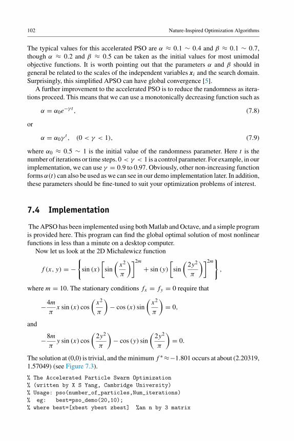
The typical values for this accelerated PSO are α ≈ 0.1 ∼ 0.4 and β ≈ 0.1 ∼ 0.7,though α ≈ 0.2 and β ≈ 0.5 can be taken as the initial values for most unimodalobjective functions. It is worth pointing out that the parameters α and β should ingeneral be related to the scales of the independent variables xi and the search domain.Surprisingly, this simplified APSO can have global convergence [5].

A further improvement to the accelerated PSO is to reduce the randomness as itera-tions proceed. This means that we can use a monotonically decreasing function such as

α = α0e−γ t , (7.8)

or

α = α0γt , (0 < γ < 1), (7.9)

where α0 ≈ 0.5 ∼ 1 is the initial value of the randomness parameter. Here t is thenumber of iterations or time steps. 0 < γ < 1 is a control parameter. For example, in ourimplementation, we can use γ = 0.9 to 0.97. Obviously, other non-increasing functionforms α(t) can also be used as we can see in our demo implementation later. In addition,these parameters should be fine-tuned to suit your optimization problems of interest.

7.4 Implementation

The APSO has been implemented using both Matlab and Octave, and a simple programis provided here. This program can find the global optimal solution of most nonlinearfunctions in less than a minute on a desktop computer.

Now let us look at the 2D Michalewicz function

f (x, y) = −{

sin (x)

[sin

(x2

π

)]2m

+ sin (y)

[sin

(2y2

π

)]2m}

,

where m = 10. The stationary conditions fx = fy = 0 require that

−4m

πx sin (x) cos

(x2

π

)− cos (x) sin

(x2

π

)= 0,

and

−8m

πy sin (x) cos

(2y2

π

)− cos (y) sin

(2y2

π

)= 0.

The solution at (0,0) is trivial, and the minimum f ∗ ≈−1.801 occurs at about (2.20319,1.57049) (see Figure 7.3).

Particle Swarm Optimization 103

104 Nature-Inspired Optimization Algorithms

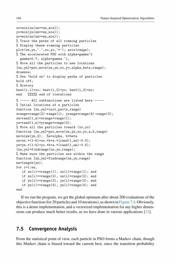
If we run the program, we get the global optimum after about 200 evaluations of theobjective function (for 20 particles and 10 iterations), as shown in Figure 7.4. Obviously,this is a demo implementation, and a vectorized implementation for any higher dimen-sions can produce much better results, as we have done in various applications [13].

7.5 Convergence Analysis

From the statistical point of view, each particle in PSO forms a Markov chain, thoughthis Markov chain is biased toward the current best, since the transition probability

Particle Swarm Optimization 105

0

1

2

3

4 01

23

4

−2

0

2

Figure 7.3 Michalewicz’s function with the global optimality at (2.20319, 1.57049).

0 1 2 3 40

1

2

3

4

0 1 2 3 40

1

2

3

4

Figure 7.4 Initial and final locations of 20 particles after 10 iterations.

often leads to the acceptance of the move toward the current global best. In addition,the multiple Markov chains are interacting in terms of partially deterministic attractionmovement. Therefore, any mathematical analysis concerning the rate of convergence ofPSO may be difficult. However, there are some good results using both the dynamicalsystem and Markov chain theories.

7.5.1 Dynamical System

The first convergence analysis in terms of dynamical system theories was carried outby Clerc and Kennedy in 2002 [2]. Mathematically, if we ignore the random factors,we can view the system formed by (7.1) and (7.2) as a dynamical system. If we focuson a single particle i and imagine there is only one particle in this system, then theglobal best g∗ is the same as its current best x∗

i . In this case, we have

vt+1i = vt

i + γ (g∗ − xti ), γ = α + β, (7.10)

106 Nature-Inspired Optimization Algorithms

and

xt+1i = xt

i + vt+1i . (7.11)

Following the analysis of a 1D dynamical system for particle swarm optimization byClerc and Kennedy [2], we can replace g∗ with a parameter constant p so that we cansee whether or not the particle of interest will converge toward p. Now we can writethis system as a simple dynamical system

v(t + 1) = v(t) + γ (p − x(t)), x(t + 1) = x(t) + v(t + 1). (7.12)

For simplicity, we focus on only a single particle. By setting ut = p − x(t + 1) andusing the notations for dynamical systems, we have

vt+1 = vt + γ ut , (7.13)

ut+1 = −vt + (1 − γ )ut , (7.14)

or

Yt+1 = AYt , (7.15)

where

A =(

1 γ

−1 1 − γ

), Yt =

(vt

ut

). (7.16)

The general solution of this dynamical system can be written as

Yt = Y0 exp[At]. (7.17)

The main behavior of this system can be characterized by the eigenvalues λ of A

λ1,2 = 1 − γ

2±√

γ 2 − 4γ

2. (7.18)

It can be seen clearly that γ = 4 leads to a bifurcation.Following a straightforward analysis of this dynamical system, we can have three

cases. For 0 < γ < 4, cyclic and/or quasi-cyclic trajectories exist. In this case, whenrandomness is gradually reduced, some convergence can be observed. For γ > 4,noncyclic behavior can be expected, and the distance from Yt to the center (0, 0) ismonotonically increasing with t . In a special case γ = 4, some convergence behaviorcan be observed. For detailed analysis, refer to [2]. Since p is linked with the globalbest, as the iterations continue it can be expected that all particles will aggregate towardthe global best.

However, this global best is the best solution found by the algorithm during iterations,which may be different from the true global optimality of the problem of interest. Thispoint will also become clearer in the framework of Markov chain theory.

Particle Swarm Optimization 107

7.5.2 Markov Chain Approach

Various studies on the convergence properties of the PSO algorithm have diverse results[2,9–12]. However, care should be taken in interpreting these results in practice, espe-cially for the discussion of the implications from a practical perspective.

Many studies can prove the convergence of the PSO under appropriate conditions,but the converged states are often linked to the current global best solution g∗ found sofar. There is no guarantee that this g∗ is the true global solution gtrue to the problem. Infact, many simulations and empirical observations by many researchers suggest that inmany cases, this g∗ is often stuck in a local optimum, which is often referred to as thepremature convergence. All these theories do not guarantee

g∗ ≈ gtrue. (7.19)

In fact, many statistically significant test cases suggest that

g∗ �= gtrue. (7.20)

According to a recent study by Pan et al. [9], the standard PSO does not guarantee thatthe global optimum is reachable, and the global optimality is searchable with a certainprobability p(ζ

(t)m ), where k is the kth iteration and m is the swarm size. Here ζ is the

state sequences of the particles.For a given swarm size m and iteration k, a Markov chain

{ξ

(k)i , k ≥ 1

}formed

by the i th particle at time k can be defined, and then the swarm state sequence ζ (k) =(ξ

(k)i , . . . , ξ

(k)m)

also forms a Markov chain for all k ≥ 1. For the standard PSO withan inertia parameter θ shown in Eq. (7.3), the probability that ζ (k+1) is in the optimalset ∗ can be estimated by

p(ζ (k+1 ∈ ∗∣∣k, m)

= 1 − p(ζ (1)) ·k∏

j=1

m∏i=1

(1 − Rk

θ ||xki − xk−1

i || · Rk

c||x∗(k)i − xk

i ||· Rk

c||g∗ − xki ||

),

(7.21)

where Rk > 0 is a local radius and c is defined by ε1, ε2 ∼ U (0, c). Pan et al. showedthat

0 ≤ p(ζ (k+1)

∣∣k, m)

≤ 1, (7.22)

which means that the standard PSO will not guarantee to get to the global optimalitynor guarantee to miss it. The equality p = 1 only holds for m → ∞ and k → ∞. Sincethe size is finite and the iteration is also finite, this probability is typically 0 < p < 1.

However, that the standard PSO does not guarantee convergence does not mean thatother variants cannot have global convergence. In fact, a recent study used the frame-work of Markov chain theory and proved that APSO can have global convergence [5].

108 Nature-Inspired Optimization Algorithms

7.6 Binary PSO

In the standard PSO, the positions and velocities take continuous values. However,many problems are combinatorial and their variables take only discrete values. In somecases, the variables can only be 0 and 1, and such binary problems require modificationsof the PSO algorithm. Kennedy and Eberhart in 1997 presented a stochastic approach todiscretize the standard PSO, and they interpreted the velocity in a stochastic sense [8].

First, the continuous velocity vi = (vi1, vi2, . . . , vik, . . . , vid) is transformed usinga sigmoid transformation

S(vik) = 1

1 + exp (−vik), k = 1, 2, . . . , d, (7.23)

which applies to each component of the velocity vector vi of particle i . Obviously, whenvik → ∞, we have S(vik) → 1, while Sik → 0 when vik → −∞. However, becausethe variations at the two extremes are very slow, a stochastic approach is introduced.

Second, a uniformly distributed random number r ∈ (0, 1) is drawn, then the veloc-ity is converted to a binary variable by the following stochastic rule:

xik ={

1 if r < S(vik),

0 otherwise.(7.24)

In this case, the value of each velocity component vik is interpreted as a probabilityfor xik taking the value 1. Even for a fixed value of vik , the actual value of xik is notcertain before a random number r is drawn. In this sense, the binary PSO (BPSO)differs significantly from the standard continuous PSO.

In fact, since each component of each variable takes only 0 and 1, this BPSO can workfor both discrete and continuous problems if the latter is coded in the binary system.Because the probability of each bit/component taking one is S(vik) and the probabilityof taking zero is 1 − S(vik), the joint probability p of a bit change can be computed by

p = S(vik)[1 − S(vik)]. (7.25)

Based on the runtime analysis of the BPSO by Sudholt and Witt [10], there are someinteresting results on the convergence of BPSO. If the objective function has a uniqueglobal optimum in a d-dimensional space and the BPSO has a population size n withα + β = O(1), the expected number N of internations/generations of BPSO is

N = O

(d

log d

), (7.26)

and the expected freezing time is O(d) for single bits and O(d log d) for nd bits.One of the advantages of this binary coding and discritization is to enable binary

representations of even continuous problems. For example, Kennedy and Eberhartprovided an example of solving the second De Jong function and found that110111101110110111101001 in a 24-bit string corresponds to the optimal solution3905.929932 from this representation. However, a disadvantage is that the Hamming

Particle Swarm Optimization 109

distance from other local optima is large; therefore, it is unlikely that the search willjump from one local optimum to another. This means that binary PSO can get stuckin a local optimum with premature convergence. New remedies are still under activeresearch.

Various studies show that PSO algorithms can outperform genetic algorithms andother conventional algorithms for solving many optimization problems. This is par-tially due to that fact that the broadcasting ability of the current best estimates givesa better and quicker convergence toward the optimality. However, PSO algorithms dohave some disadvantages, such as premature convergence. Further developments andimprovements are still under active research.

Furthermore, as we can see from other chapters in this book, other methods such asthe cuckoo search (CS) and firefly algorithms (FA) can perform even better than PSOin many applications. In many cases, DE, PSO, and SA can be considered special casesof CS and FA. Therefore, CS and FA have become an even more active area for furtherresearch.

References

[1] Chatterjee A, Siarry P. Nonlinear inertia variation for dynamic adaptation in particle swarmoptimization. Comp Oper Res 2006;33(3):859–71.

[2] Clerc M, Kennedy J. The particle swarm. Explosion, stability, and convergence in a mul-tidimensional complex space. IEEE Trans Evol Comput 2002;6(1):58–73.

[3] Engelbrecht AP. Fundamentals of computational Swarm intelligence. Hoboken, NJ, USA:Wiley; 2005.

[4] Gandomi AH, Yun GJ, Yang XS, Talatahari S. Chaos-enhanced accelerated particle swarmoptimization. Commun Nonlinear Sci Numer Simul 2013;18(2):327–40.

[5] He XS, Xu L, Yang XS. Global convergence analysis of accelerated particle swarm opti-mization. Appl Math Comput [submitted, Sept 2013].

[6] Kennedy J, Eberhart RC. Particle swarm optimization. In: Proceedings of the IEEE inter-national conference on neural networks, Piscataway, NJ, USA; 1995. p. 1942–48.

[7] Kennedy J, Eberhart RC, Shi Y. Swarm intelligence. London, UK: Academic Press; 2001.[8] Kennedy J, Eberhart RC. A discrete binary version of the particle swarm algorithm. Inter-

national conference on systems, man, and cybernetics, October 12–15, 1997, Orlando,FL, vol. 5. Piscataway, NJ, USA: IEEE Publications; 1997. p. 4104–9.

[9] Pan F, Li XT, Zhou Q, Li WX, Gao Q. Analysis of standard particle swarm optimizationalgorithm based on Markov chain. Acta Automatica Sinica 2013;39(4):381–9.

[10] Sudholt D, Witt C. Runtime analysis of a binary particle swarm optimizer. Theor ComputSci 2010;411(21):2084–100.

[11] Trelea IC. The particle swarm optimization algorithm: convergence analysis and parameterselection. Inf Process Lett 2003;85(6):317–25.

[12] van den Bergh F, Engelbrecht AP. A study of particle swarm optimization particle trajec-tories. Inf Sci 2006;176(8):937–71.

[13] Yang XS, Deb S, Fong S. Accelerated particle swarm optimization and support vec-tor machine for business optimization and applications. In: Networked digital technolo-gies. Communications in computer and information science, vol. 136. Berlin, Germany:Springer; 2011. p. 53–66.

110 Nature-Inspired Optimization Algorithms

[14] Yang XS, Gandomi AH, Talatahari S, Alavi AH. Metaheuristics in water. In: Geotech TransEng. Waltham, MA, USA: Elsevier; 2013.

[15] Yang XS, Cui ZH, Xiao RB, Gandomi AH, Karamanoglu M. Swarm intelligence andbio-inspired computation: theory and applications. London, UK: Elsevier; 2013.