nature and nurture effects on children's · pdf filenature and nurture effects on...
TRANSCRIPT

1
NATURE AND NURTURE EFFECTS ON CHILDREN'S OUTCOMES: WHAT HAVE WE LEARNED FROM STUDIES OF TWINS AND ADOPTEES?*
Bruce Sacerdote
Dartmouth College and NBER
This Version: February 27, 2008
* I thank Christopher Jencks, Anders Björkland, and seminar participants at NYU for their comments on this literature summary. I thank Holt International Children's Services and particularly Laura Hofer and Karla Miller for their help in gathering data and information on international adoptions. The National Science Foundation provided generous funding. I thank Celia Kujala, Anne Ladenburger, Abigail Ridgeway, and Ariel Stern for tireless research assistance and valuable suggestions.

2
I. Introduction and Overview
A fundamental question in social science has long been the degree to which
children's outcomes are influenced by genes environment, and the interaction of the two.
One sensible way to attempt to separate out the effects of genes and environment is to
examine data on twins or adoptees since we may be able to make plausible assumptions
about the genetic relationships between identical versus fraternal twins or between
parents and their adoptive and non-adoptive children.
I begin this chapter by reviewing the methods used by psychologists and
behavioral geneticists to identify the effects of nature and nurture and I summarize some
of the key results from this large literature. I discuss the assumptions underlying the
behavioral genetics model and explain some of the challenges to interpreting the results.
I use these issues of interpretation to motivate why economists and sociologists have used
a different approach to measuring the impact of environment on children's outcomes.
And I discuss the results from the recent literature in economics on environmental versus
genetic determinants of children's education, income and health. Finally I try to bring the
results from both literatures together to address the issues of what we do know, what we
don't know and whether any of this work has implications for social policy or other
research on children's outcomes.
Behavioral geneticists have estimated the "heritability" of everything from IQ to
"shrewdness" to alcoholism. Their most frequently cited result is that genetic factors
explain about 50 to 60 percent of the variation in adult IQ while family environment
explains little of the variation in adult IQ1. This finding is incredibly robust (see Devlin
at al [1997]). But researchers' interpretation of the finding is all over the map. Harris
[1998] uses the finding of almost no effect from family environment as a key piece of
1 Studies of young adoptee's IQ find significant effects of family environment, though still only 1/3 as large as the genetic effects. See Cardon and Cherny [1994]. These effects of adoptive family environment appear to be attenuated in adulthood and get even smaller in old age. Plomin et al [2001].
3
evidence for her thesis that parents do not have a direct effect on their children's
outcomes. And both Hernnstein and Murray [1994] and Jensen [1972] interpreted the
lack of measured effect from family environment to mean that policies aimed at
improving the home and school environment of children are likely to have small impacts
on outcomes.
Jencks et al [1972], Jencks [1980] and Goldberger [1977] provide a series of
reasons why such strong interpretations may be unwarranted. First of all, understanding
the determinants of IQ is different than understanding the determinants of educational
attainment, income and health. Second, the assumptions of the behavioral genetics model
are likely tilted towards overstating the importance of genes in explaining variation in
outcomes. Positive correlation between family environment and genes raises the
heritability estimate. Third, family environment is likely endogenous and may depend
heavily on genes (Jencks [1980], Scarr and McCartney [1983], Dickens and Flynn
[2001]). This endogeneity makes any simple nature nurture breakdown difficult to
interpret. Fourth, noting that variation in a given outcome for some population has a
large genetic component is very different from saying that the outcome is predetermined
or cannot be changed by interventions. Genetic effects can be muted just as
environmental effects can be. To take Goldberger's example, a finding that most of the
variation in eyesight is due to genes does not imply that we should stop prescribing
eyeglasses for people. The use of eyeglasses may add enormous utility for people (and
offer an excellent return on investment), regardless of what fraction of eyesight is
measured as being environmental.
In other words, knowing what fraction of the existing variance is environmental
does not tell us whether a given environmental intervention is doomed to failure or
success. Imagine a state with uniformly mediocre schools. Perhaps in that population,
school quality doesn't explain any of the variation in student outcomes. But there may be
great benefits from introducing a new school with motivated peers, high financial
resources and high teacher quality. It is critical to bear in mind that the variance
breakdown only deals with variation in the sample. Mechanically, expanding a sample to
4
encompass a broader range of environment (eg considering children in both Africa and
the US as opposed to the US alone) will increase the variation in inputs and outcomes and
likely the proportion of the variation in outcomes that is due to environment.
The precision and specificity with which one must properly interpret behavioral
geneticists' estimates lead Jencks [1972] to write that "indeed our main conclusion after
some years of work on this problem is that mathematical estimates of heritability tell us
nothing about anything important." In his analysis Goldberger [1978] summed up by
noting that "such conclusions [of high genetic influence on schooling] are unwarranted
and indeed the entire effort is misguided." Feldman and Otto [1997] note that obtaining a
plausible decomposition has proven notoriously elusive and that we do not know the
correct model to use for any given trait.
These warnings from these highly esteemed authors from three separate
disciplines (sociology, economics and biology) should be enough to make other social
scientists realize that we cannot simply take the estimates from behavioral genetics and
plug them into a causal model of children's outcomes or to predict the effect of some
policy intervention. In fact, economists are probably right to ignore the importance of
genetic factors when studying any particular policy or law change since a policy can have
meaningful or tiny effects (or could represent a great or terrible return on investment)
regardless of the measured heritability of the outcome.
What then do we learn from behavioral geneticists' estimates of the relative
contribution of genes, family environment and non-shared environment? We are getting
a breakdown of the variance of the outcome in the current population, assuming a
particular structural model. In the case of adoption studies, heritability is a measure of
how much more biological siblings resemble each other relative to adoptive siblings.
Similarly in the case of twin studies, heritability is a measure of how much more
outcomes for identical twins are correlated relative to outcomes for fraternal twins or
other siblings. See the next section for the algebra. If heritability estimates were labeled
as the additional correlation in outcomes that is associated with being identical rather

5
than fraternal twins, there might be less misinterpretation and less obsession with these
numbers.
Such a variance breakdown may be worth something to social scientists to the
extent that they want a best estimate as to whether genetic variation is particularly
important in determining an outcome. Even if the functional form of the behavioral
genetics model is terribly simplified or wrong, the model might still deliver useful
relative rankings of how much variation in genes contributes to variation of different
outcomes (e.g. height versus age at first marriage.) The breakdown of outcome variance
into variance contributed by genes, family environment and non-shared environment is an
ambitious goal, but one that comes with many caveats and questions of interpretation.
Economists and sociologists have suggested several ways to reframe the question
so as to use adoption data to estimate some of the causal impacts from family
environment without having to know the true model by which outcomes are determined
and without having to deliver a complete nature, nurture breakdown. This line of
research consists of regressing child outcomes on parental characteristics, i.e. using the
more standard approach within economics. For example Plug and Vijverberg [2003] and
Sacerdote [2007] regress adoptee's years of schooling on mother's years of schooling,
family income and family size. The advantage of using regression is that it tells us which
specific parental inputs are most correlated with child outcomes and slope of the
relationships.
Certainly one cannot necessarily take these regressions coefficients as causal due
to measurement error, endogenous relationships among the right hand variables, and
unobservables. But these regressions provide a starting point for understanding which
parental inputs matter and how they matter much even in the absence of a genetic
connection between parents and children. We can then compare the observed
coefficients on parental inputs that we find for adoptees to those that use other sources of
variation in family characteristics. For example, Sacerdote [2007] finds little evidence
for a direct effect of parental income on adoptees' income and education and this is

6
generally consistent with the work of Mayer [1997] and Blau [1999].2 And one can
compare the effects of family size found in adoption studies to those found by Black
Devereux and Salvanes [2005b] and Angrist, Lavy and Schlosser [2005] who use the
birth of identical twins and sex preferences as an exogenous shock to family size.
One can also generate separate transmission coefficients for adoptees and non-
adoptees by regressing the child's outcome on that of the parent. See Björklund Lindahl
and Plug [2006] and Björklund Jäntti and Solon [2007] for transmission coefficients of
income (education) from parents to adoptees and nonadoptees. This enables one to see
how transmission varies when there is and is not a genetic link to the parents. This work
also carries the advantage of providing comparability between existing estimates of
transmission coefficients from parents to children such as those in Solon[1999],
Zimmerman [1992] and Mazumder[2005].
Several bottom lines emerge from my summary of the nature and nurture
literature. First, economists who are not already familiar with the literature are generally
surprised by how much genes seem to matter, or more precisely stated, how much less
adoptees resemble their adoptive parents and siblings than do nonadoptees.3 Second, the
estimated effects of family environment on adoptee outcomes are still large in some
studies and leave tremendous scope for children's outcomes to be affected by changes in
family, neighborhood or school environment. And the importance of family environment
can rise significantly when the model is made more flexible.
Third, the precise breakdowns of variance provided by behavioral genetics are
subject to a number of important issues of interpretation. Findings of little variance
contribution from family environment to variance in children's IQ or educational
attainment might be partially generated by the model's assumptions and in any case do
not necessarily imply that interventions in environment will not affect child outcomes or
that parents actions do not have a direct impact on child outcomes. Finally, the
2 Mayer [1997] does find evidence for an effect of parental income on college attendance. 3 In the twins literature, one might say that economists are often surprised by how much more similar are outcomes for identical twins relative to fraternal twins.

7
importance of adoptive family characteristics for adoptee outcomes varies significantly
depending on which outcomes are considered. For example, college selectivity and
drinking habits seem to be significantly more influenced by adoptive family
characteristics than are test scores.
Ultimately the evidence is quite consistent with the simplistic and widely held
view that both nature and nurture matter a great deal in determining children's outcomes.
Parental characteristics matter a great deal even in the absence of any genetic connection
to their children. A more deeply informed view will also recognize that certain
measured parental effects or transmission coefficients from parents to children drop
significantly when one considers adoptees rather than children raised by their biological
parents. However, that fact does not negate any of the findings of researchers who
measure directly the causal effects of changing school, neighborhood and family
environment on outcomes.
II. The Behavioral Genetics Model4
In the simplest version of the model, child outcomes (Y) are produced by a linear
and additive combination of genetic inputs (G), shared (common) family environment (F)
and unexplained factors, which the BG literature often calls non-shared or separate
environment, (S). This implies that child's educational attainment can be expressed as
follows
(1) Child's years of education (Y)= G + F + S
The key assumptions here are that nature (G) and shared family environment (F)
enter linearly and additively. Separate environment (S) is by definition the residual term
4 Large portions of the text here are copied from Sacerdote [2007].

8
and is uncorrelated with G and F. In the simple version of the model one further assumes
that G and F are not correlated for a given child. On the surface, this seems like a strange
assumption and one that could perhaps be defended for some subsets of adoptees but not
for children being raised by their biological parents. At a deeper level, behavioral
geneticists often take F to represent that portion of family environment which is not
correlated with genes and they assume that G represents both the effects of gene and
gene-environment correlation. The correlation between G and F can be modeled
explicitly. If F itself is endogenous, modeling becomes very difficult. With these caveats
in mind, one can already see that the BG breakdown into genes versus family
environment is not necessarily an easily interpreted decomposition.
With the assumptions of no correlation between G,F, and S, taking the variance of
both sides of equation one yields:
(2) σ2Y = σ2
G + σ2F + σ2
S
Dividing both sides by the variance in the outcome (σ2y ) and defining h2 =σ2
g
/σ2y, c2 =σ2
F /σ2y , and e2 = σ2
S /σ2Y yields the standard BG relationship:
(3) 1 = h2 + c2+ e2
The variance of child outcomes is the sum of the variance from the genetic inputs
(h2 or heritability), the variance from family environment (c2) and the variance from non-
9
shared environment (e2), i.e. the residual. From this starting point, a variety of variances
and covariances of outcomes can be expressed as functions of h, c, and e. The sample
moments can then be used to identify these underlying parameters. Consider first the
relationship for two adoptees. If one standardizes Y,F,G,S to be mean zero variance one,
the correlation in outcomes between two adoptive siblings equals
(4) Corr (Y1, Y2) = Cov(Y1,Y2)=Cov(F1,F1)=Var(F1)=c2.
The correlation in outcomes between two nonadoptive siblings equals
(5) Corr (Y1, Y2) = Cov (G1+F1+S1, G2+F2+S2) = Cov (G1+F1, 1/2G1+F1) = ½ h2 + c2.
This assumes that non-adoptive siblings share half of the same genetic endowment and
the same common environment (See Plomin et. al [2001] for a discussion). Thus one
can recover the full variance breakdown (h2,c2,e2) from just the correlation among
adoptive and biological siblings. By comparing (4) and (5) we see that h2= twice the
difference in correlations in the outcome between the adoptive and biological siblings.
This is the "double the difference" methodology frequently referred to in text books or
discussions of the BG model (See Duncan et al [2001]).
Now consider the correlation in outcomes between two identical twins versus the
correlation for two fraternal twins. Identical twins are assumed to share all of the same
genes and the same family environment and hence their correlation in outcomes is
(6) Corr (Y1, Y2) = Cov (G1+F1+S1, G2+F2+S2) = Cov (G1+F1, G1+F1) = h2 + c2.
The algebra for the fraternal twins is the same as the algebra for any two biological
(nonadoptive) siblings and hence the same ½ h2 + c2 we had in the preceding paragraph.
By subtracting (5) from (6) and multiplying by 2, we see that h2 is twice the difference in
10
correlations between identical and fraternal twins. Thus the twins literature has its own
"double the difference" methodology.
Of course one need not stop at finding the analytical solutions for the correlations
for just twins, adoptive siblings and full siblings. One can also write down the equations
for correlations in outcomes between children and parents, grandchildren and
grandparents, between first cousins etc. This general model is known as Fisher's
Polygenetic Model. Behrman and Taubman [1989] provides a great illustration in that
the authors present formulae for the phenotypic (outcome) correlations among 16
different possible pairings of relatives.
Note that as we add more pairings of different relatives, we can incorporate
additional parameters and potentially make the model more realistic. (We can add
flexibility and identify additional structural parameters.) Goldberger [1977] provides
examples of models which allow for gene-environment correlation and use correlations
among twins reared together, twins reared apart, adoptive siblings, and the parent-child
correlations for twins and adoptees. Frequently the structural models employed are
overidentified (because there are more pairings of relatives than parameters) in which
case the estimation chooses parameters which minimize the sum of squared errors
between the sample moments and the fitted values of the sample moments.
In the case of Behrman and Taubman's [1989] model, they allow both for the
possibilities of assortative mating and for the effects of dominance versus additive genes.
Assortative mating is the notion that couples may positively select on phenotypes
(outcomes), ie. mating is non-random which means that siblings may have more than
50% of the same genes. Dominant gene effects are identified separately from additive
effects by comparing correlations in outcomes across types of relatives that would have
the same genetic connection under an additive system but need not if dominant effects are
present. For example, suppose we had data for full siblings, half siblings and identical
twins and we assume that all sibling pairs receive the same common environment. Think
of the difference in correlation between full siblings and half siblings as identifying the

11
effects of genetic connection. Under an additive system, genetic effects will cause
exactly twice as much resemblance in identical twins as is caused among full siblings. If
identical twins resemble each other MORE than twice as much as implied by the other
sibling types, one could attribute this "additional" component to the dominance effects of
genes.5 Behavioral geneticists may also want to allow for the interactive effects of
different genes which is known as epistasis. By modeling the correlation among even
more pairings of relatives (beyond the three types of sibling pairs mentioned above), one
can have additive genetics effects, dominance effects and epistasis in the same model.
Note that there are at least three other ways in which the structural modeling can
be further extended. First one might assume that the same underlying process gives rise
to several different outcomes. For example, one might have two verbal test scores on the
same set of individuals. One could treat these as yielding two sets of sample moments
which can be used to identify the same underlying parameters. Alternatively, one might
have a panel of test score outcomes for the same group of relatives over time and one
could posit that the relationship between siblings' outcomes is changing over time in a
specific way. See Cardon and Cheny [1994]. Finally one can also allow for different
levels of gene-environment correlation among different relatives (e.g. fraternal and
identical twin pairs need not be modeled as having correlation of 1.0 in their family
environments.)
An important assumption in this modeling is that the various samples used to
estimate the relevant covariances have the same underlying variance in genes and family
environment. If for example, adoptive families have a restricted range of family
environments (Stoolmiller [1999]), then it may not make sense to combine covariances
from adoptive siblings, non-adoptive siblings and twins all in the same estimation.
Furthermore, the variance breakdown obtained using adoptees may not apply to the
general population.
5 Goldberger [1977] page 331 offers the following intuition: "If the individual genes have non-additive effects, then it is only the additive part of the effect that makes for parent-child resemblance. The non-additive part of the effect does contribute to the resemblance of siblings, who may happen to receive the same gene combination."

12
In practice, the results are sensitive to which relative pairs are modeled in the
analysis. As noted above, a great deal of weight is often placed on the difference in
correlations of outcomes for adoptive siblings versus full siblings or for fraternal versus
identical twins. However, if we instead compare parent-child (i.e. intergenerational)
correlations to sibling correlations, we get a different answer for h2 , c2, e2 than if we
compare across sibling types. Solon [1999] notes that the sibling correlation equals the
sum of the intergenerational correlation squared plus other shared factors, all of which are
nurture based. Björklund and Jäntti [2008] points out that sibling correlations in many
outcomes are typically much higher than intergenerational correlations. And they show
that this fact combined with the BG model implies a large nurture based component to
outcomes.
III. Canonical Results from the Behavioral Genetics Literature
As noted earlier, the most voluminous and heavily cited part of the BG literature
measures the contributions of genes and family environment to IQ. There are numerous
summaries of this IQ literature including Goldberger [1977], Bouchard and McGue
[1981], Devlin [1997], Jencks et al [1972], and Taylor [1980]. Table I shows the mean of
the estimated correlations in each of these meta-studies along with the number of
individual studies incorporated.
Devlin, Daniels and Roeder reviewed 212 different studies of the IQ of twins.
The mean correlation in IQ for studies of pairs of identical was .85. The correlations for
fraternal twins were similar to correlations for other siblings and averaged .44. One can
see immediately that in a simple model this will generate a high estimated heritability; if
one assumes that identical twins are twice as genetically related as other full siblings and
have twice the correlation in outcomes, equations (5) and (6) would lead one to conclude
that all the explained variance is genetic. Goldberger (1977) and Jencks et al [1972] each
reviewed a number of twins studies of IQ. The studies they review yielded similar

13
results. In the case of Jencks [1972], the correlation in IQ for identical twins is .86 versus
.54 for other siblings.
Bouchard and McGue [1981] examined a large number of twin studies and
adoption studies. The adoption studies find significant correlation in IQ between
adoptive siblings. The median correlation in IQ for adoptive siblings is .29 while the
correlation for biological siblings raised together is .45. However, many of these studies
are for adoptees less than age 18. Studies of older adoptive and biological siblings have
found that the correlation in IQ among adoptees tends to fall significantly in adulthood
while the correlation for biological siblings grows. Plomin et al [1997, 2001].
Table II translates these sibling correlations into the behavioral genetics
decomposition of variance in IQ into portions attributable to variance in genes, family
(common) environment and separate environment. The twins designs find that a high
proportion of explained variance in IQ is due to genes and very little is due to family
environment. Averaging over more than 200 studies, Devlin et al show the average
finding is that 49 percent of the variance is genetic and 5 percent is attributable to family
(common) environment. The Bouchard and McGue summary of correlations for twins
finds similar results, namely that 54 percent of variation is genetic and 4 percent is due to
family environment. Non-shared environment (what economists would call the residual
or unexplained variance) accounts for a substantial 40-50% of the variation in IQ.
The adoption studies find a larger proportion of variance in IQ attributable to
family environment. Cardon and Cherny's [1994] examination of nine year olds in the
Colorado Adoption Project found that 16 percent of the variation in IQ is attributable to
family environment and 60 percent is due to genes. The Bouchard and McGue summary
of IQ correlations for adoptees implies that 29 percent of the variation is due family
environment and 32 percent is due to genes. Averaging over the studies in Goldberger's
[1977] literature summary which includes both twin and adoption correlations, I find that
22 percent of the variation in IQ is due to family environment and 58 percent is due to
genetic effects.

14
There is a disconnect between the twin and adoption literatures with regard to the
importance of family environment. One way to partially resolve this contradiction is to
appeal to the findings that family environment effects on adoptees are greatly attenuated
in adulthood and that heritability rises with age (Pedersen et al [1992] and McClearn et
al [1997]). However, another reasonable explanation is that applying the simple version
of the behavioral genetics model to pairs of identical and fraternal twins will overstate
heritability if identical twins face environments more similar than that faced for other
siblings (Feldman and Otto [1997].)6 Or identical twins might affect each other's
environment more than do fraternal twins. Recall from section II that any factors which
make outcomes for identical twins more similar than outcomes for fraternal twins are
assigned to genetic effects. The assumption of the structural model is that sibling pairs
raised in the same household have the same correlation in family or common
environment. One could imagine that parents and teachers would be even more likely to
expect or demand similar performance from siblings who are identical twins. Parents
may be more likely to provide similar environmental experiences for identical twins. In
decomposing sources of earnings variation, Björkland Yäntii and Solon [2005] find that
allowing different types of sibling pairs to have different amounts of correlation in family
environment greatly lowers the estimated heritability and raises the estimated impacts
from family environment.
In Table III, I summarize the existing behavioral genetics studies of variance in
years of education. There are far fewer BG studies of education and earnings than of IQ,
and the most widely known studies are those done by economists and sociologists.
Behrman and Taubman [1989] uses data on twins and their relatives from the National
Academy of Science / National Research Council sample. They compute years of
schooling correlations for 16 different pairs of relatives and fit the parameters of their
model to match the predicted correlations with the sample correlations. Consistent with
twins studies of IQ that find high heritability, Behrman and Taubman find that genetic
6 Scarr and Carter-Saltzman [1979] provide some evidence that identical and fraternal twins do have similar correlations in family environment.

15
effects explain 88 percent of the variation in schooling.7 Family environment explains
little or none of the variance in schooling. Scarr and Weinberg [1994] examine adoptees
and find that family environment explains 13 percent of the variation. However, this
study is based on only 59 adoptive sibling pairs. Teasdale and Owen [1984] have 163
pairs of adoptees and find that variance family environment explains 5 percent of the
variation in schooling.
Overall, to the extent that behavioral geneticists have performed nature-nurture
decompositions using years of schooling as the outcome, the findings have mirrored the
findings of the much larger IQ literature. Genetic effects play a large role while there is
only a small role for family environment. That statement is tempered a bit by the
Behrman, Taubman and Wales study and Scarr and Weinberg study, though that study
had only 59 pairs of adoptive siblings. A different but equally valid interpretation of the
results in Table III would be to say genetic effects clearly matter a great in determining
schooling, but that the portion attributable to family environment changes significantly
depending on how one specifies the structural model.
In Table IV I switch the outcome of interest to earnings and I report results from
two different studies. Björkland, Jäntti and Solon [2005] used a large sample of siblings,
twins and adoptees from the Statistics Sweden and Swedish Twin Registry. They derive
formulae for the predicted correlations among nine different sibling types. They use
weighted least squares to choose parameters to best fit the sample correlations to the
predicted correlations from the models. One of the key results from this study is that it
matters a great deal whether or not one constrains all sibling types reared together to have
the same degree of correlation in family (common) environment. With such a constraint
(Model 1), genes explain 28 percent of the variance in earnings and family environment
explains 4 percent.8 By adding three additional parameters to allow for differing
correlations in family environment among sibling pairs (Model 4), the importance of 7 The earlier Behrman Taubman and Wales [1975] study used the same data set of twins, but found lower heritability of schooling. This may be precisely because of the different way the two studies modeled correlation in family environment. 8 These are the numbers for brothers. For sisters, the comparable numbers are 24.5 percent genetic and 1 percent common environment.

16
family (common) environment rises to 16.4 percent and the genetic effects fall to 19.9
percent.
Table V shows the results from Loehlin's [2005] summary of the behavioral
genetics literature on the determinants of personality traits. Like the IQ research, this is a
rich literature and Loehlin considers hundreds of studies. He reports average correlations
between parents and children for the most commonly measured aspects of personality,
namely extraversion, agreeableness, conscientiousness, neuroticism, and openness. With
regard to the determinants of personality traits, the literature has reached even more of a
consensus than with regard to IQ. The first column is for the correlations between
parents and children when children are raised by their biological parents. Correlations
range from .11 to .17. When we consider adoptees and adoptive parents in column 2, the
correlations almost disappear, falling to an average of .036. Column 3 reports
correlations in traits for adoptees and their biological parents. Here the correlations rise
almost to the levels seen in column (1), ie for the children raised by their biological
parents. This evidence (which again is a summary of hundreds of studies) is striking and
certainly points strongly in the direction of genes being an important determinant of
personality traits.
As a final outcome of interest, I graph in Figure I some of the data from the Grilo
and Pogue-Geile [1981] meta study of correlations in weight, height and body mass index
among full siblings raised together, adoptive siblings, and twins. Adoptive siblings have
almost no correlation in body mass index. Full siblings raised together have a correlation
of about .32. Interestingly fraternal twins show similar levels of correlation to other
sibling pairs. The correlation in BMI jumps to .72 for identical twins.9
IV. Critiques and Challenges to Interpretation of the Behavioral Genetics Results on
IQ and Schooling
9 I report the body mass index correlations which combine data for both same and mixed gender pairs of siblings. It would look only moderately different if I controlled for gender.

17
BG results with respect to IQ appear to be quite robust in finding that the genetic
effects account for 50 to 60 percent of the variance in adult IQ. In the twins studies and
the studies of adult adoptees, family environment accounts for almost none of the
variance.10 Behrman and Taubman [1989] and Teasdale and Owen [1989] find no role
for family environment in explaining years of schooling. What is one to make of these
findings? One approach is to accept this finding as not only an accurate estimation of the
BG model, but also as having important causal meaning and predictive power for
interventions which might affect child test scores, educational attainment or income.
This is the approach of Jensen [1973] and Murray [2004] who are pessimistic about the
ability of social policy to affect inequality of income and schooling.
This view is unsatisfying not only because it makes one unpopular at dinner
parties, but more importantly because such conclusions about the real weakness of family
influences and other forms of environment like school quality seem to contradict
everyday experience. And it is hard to reconcile a view of minimal effects of shared
environment with the extensive investments that many parents and school systems make
in their children.11 For example, there is a widespread belief that certain charter schools
and certain Catholic schools have large treatment effects on test scores and high school
graduation rates. These beliefs have been subsequently confirmed by very careful
empirical work on the treatment effects from these schools. See Hoxby and
Murarka[2007], Evans and Schwab [1995], and Neal[1997].
One way to handle the apparent contradiction is to note that some BG estimations
(particularly those using adoption data for younger adoptees) find a significant role for
shared environment in determining income, IQ and education. Perhaps many of the well
measured treatment effects of interventions are working through the 15-20% role
10 Some of the studies of younger adoptees find that up to 16% of the variation in child IQ is attributed to family environment (Cardon and Cherny [1994]). This clearly leaves the question of family environment effects on test scores open to interpretation. Nonetheless both Harris [1998] and Plomin et al [2001] p. 176 sum up the literature by stating that effects of family environment on IQ are modest and get smaller or disappear with age. 11 I am assuming here that a large part of school quality is shared between siblings, which strikes me as a reasonable assumption. Parents may of course invest in children for reasons besides producing higher income and levels of education.

18
assigned to shared environment. In the large Devlin et al meta study for twins data, the
consensus number for the variance explained by family environment is 5%. But the older
literature summary by Goldberger [1977] implies an average percent explained by family
environment of 22%.
A different approach to reconcile the observed environmental effects on test
scores and schooling with the BG decomposition is to note that behavioral geneticists
may be working only within a restricted range of environments that are actually observed
in the United States or in some other society. Stoolmiller [1999] emphasizes this point
and presents corrections for this "restriction of range" problem.
This is certainly a correct and incredibly important point. A variance
decomposition only deals with the variance observed in the data. In Sacerdote [2007], I
study Korean American adoptees who were places as infants with US families. Clearly if
I extended the sample to included adoptees who remained in Korea, then the variance of
educational attainment would rise substantially as would (in all likelihood) the portion
attributable to environmental factors such as home country. A less extreme example
might be to say that while Catholic schools may represent shared environment and may
have large effects, Catholic schools are not an important source of variation in the BG
studies being considered.
A third and popular reaction to the key BG findings is that one needs to somehow
fix the BG structural model so that it not only delivers more plausible estimates of the
effects of shared environment, but can also explain other facts such as the Flynn effect.
Flynn [1999] notes that IQ scores tend to rise over time. Dickens and Flynn [2001]
present an elegant model in which environment responds endogenously to genetic
endowments. This can explain a number of facts including the Flynn effect and possibly
why the effect of adoptive parents on adoptee's IQ diminishes in adulthood. The
Björklund, Jäntti Solon [2005] decomposition for earnings finds that heritability falls
significantly once they allow for different shared environment correlations among
identical twins relative to fraternal twins. Following this logic, one could either conclude
19
A) that the whole enterprise is not robust to modest changes in how we write down the
structural model or B) once we make the model a bit more flexible we arrive at a fairly
accurate and useful structural model.12
More generally there is a sizable literature that points out that gene environment
interactions or the endogeneity of environment will cause the BG model to understate the
importance of shared environment and overstate the importance of genetic factors. See
Ridley [2003] or Turkheimer [1997]. Turkheimer et al. [2003] makes the point that
nonlinearities in the relationship between genetic factors and outcomes can cause the BG
model to overstate heritability. In particular they find that measured heritability is lower
for children in less advantaged families. Lizzeri and Siniscalchi [2007] point out that if
parents are behaving optimally, the learning process for adoptees and nonadoptees will
likely differ and that this can lead behavioral genetics' estimates to greatly overstate
heritability.
I suggest another approach to understanding the BG results on IQ, schooling and
income. This approach follows that of Jencks et al [1972], Goldberger [1977] and
Duncan et al [2001]. Rather than further trying to "fix" the BG model, let's just accept
that this is a simple structural model with strong assumptions and that the model may not
be able to deliver causal, out of sample predictions about the effects of the type of
environmental interventions of interest to social scientists The facts from the BG work
are that nonadoptive siblings (identical twins) resemble each other much more on certain
outcomes than do adoptive siblings (fraternal twins). Clearly that suggests that genes
matter a lot. We need not proceed from this fact to a full decomposition of outcome
variances into the effects of genes which we do not observe and a single index of shared
environment which we do not observe. And if we do implement such a decomposition,
one needs to keep in mind that we are decomposing variance within the sample that we
have; the causal effects for interventions outside of this range may be bigger or smaller
than effects implied by the decomposition. And finally if even if we had the ultimate
12 To the extent that all we have done is add parameters to the model until we get a decomposition that fits our priors, the approach would not be useful for making predictions or explaining other puzzles.
20
decomposition, it is unclear that it could be used to make out of sample predictions about
the effects of policy changes or the degree to which a shock to an individual will affect
her children.
V. Enter the Economists and Sociologists: Treatment Effects and Regression
Coefficients
Economists tend to be much more interested in the associations and causal
relationships among variables that we do observe, such as parental income and children's
schooling. And we tend to study children's health, income, education, marital status and
happiness as the outcomes of interest rather than IQ scores and personality traits.
Rubin's causal model [1974] provides an excellent framework for understanding
and clarifying what is meant by a "causal effect" or a "treatment effect." According to
Rubin (and many empirical economists), in order to measure a causal effect there needs
to be an identifiable intervention that could implemented or not implemented. The causal
effect of the treatment on outcome Y for unit i is the difference in potential outcomes that
will occur with versus without the treatment being applied. Thus one wouldn't measure
the causal effect from being black or female since that it is not a treatment one could
apply or withhold. Similarly, one cannot interpret the BG variance decomposition in a
strict causal sense since one cannot literally alter the subjects' genes. Nor can one
actually move the family environment of a twin or an adoptee by a standard deviation of
the BG index of shared (family) environment since this index is a theoretical concept and
not observed.
I take this point very literally in Sacerdote [2007] in which I reduce the problem
to estimating the causal effect from an adoptee being assigned to one type of family
versus another. For example, I calculate the effects on adoptee's educational attainment
from being assigned to a family in which both parents have college degrees and there are
three or fewer children in the family. More formally I estimate:

21
(7) Ei= α + β1*T1i + β2*T2i + Malei + Ai + Ci + εi
Where Ei is educational attainment for child i, T1i is a dummy for being assigned
to a family with three or fewer children and high parental education, T2 is a dummy for
being assigned to a family that either has three of fewer children OR has one or more
college educated parents, Ai is full set of single year of age dummies, and Ci are a full set
of cohort (year of adoption) dummies. The omitted category are children assigned to
large families in which neither parent has a college education.
This has the clear disadvantage of only identifying the effect of a discrete jump in
family characteristics like parental education that have more variation than simply
"college degree or not." However, the advantage is that the result is very easy to explain
and interpret. β1 is the causal effect on outcomes from being assigned to a particular
family type. The family type includes size, parental education and all the observables
and unobservables correlated with those two characteristics.13 In such an analysis, there
is no attempt to make broader statements about the effects of genes or an overarching
index of family environment.
Random assignment of adoptees to families plays a critical role in this analysis. It
is the lack of correlation between adoptee pre-treatment characteristics and adoptive
family characteristics that allows one to give β1 a causal interpretation.
More broadly, economists and sociologists have used regression to estimate the
effects of child and adoptive family characteristics on adoptee outcomes. Examples of
this include Plug and Vijverberg [2003], Scarr and Weinberg [1978] and Sacerdote
[2002]. A typical equation estimated is of the form:
13 For example, the adoptive families that are large and in which neither parent has a college education may have very different unobserved characteristics that the other families. The quality of the school system might be different or the amount of time spend reading to children might be different, β1 and β2 will incorporate effects from such unobserved characteristics.

22
(8) Ei= α + β1*MomsEdi + β2*DadsEdi + β4*Log(Family Income)i + β5*Birth Orderi+
β6*Malei + εi
Here Ei represents adoptee i's years of education while MomsEdi and DadsEdi represent
adoptive mother and adoptive father's years of education. If one had similar measures for
the biological mother and father, those could clearly be added to the equation as well.
This approach loses the bare simplicity of the treatment effects approach in
equation (7) but gains a great deal in allowing the reader to think about which adoptive
family (or biological family) characteristics are most correlated with adoptee outcomes
and how steep the slopes are. Social scientists have long used regression to attempt to
separate out the effects of different right hand side variables. Clearly selection,
measurement error, collinearity and unobservables can potentially bias β1-β4 away from
the true treatment effects. But these caveats are well understood and presenting the
results in the form of regression coefficients is transparent.
Furthermore, the use of regression coefficients in studying the effects of adoptive
family characteristics allows a direct comparison of the results to other studies that
attempt to hone in on particular and exogenous shock to family environment. For
instance Blau [1999] and Meyer[1997] present evidence that shocks to income itself have
only small effects on child education and income. The results from adoption studies
appear to confirm this finding (see the following section).
The final and most common approach used by economists is to calculate
transmission coefficients of various outcomes from adoptive and biological parents to
adoptees. A transmission coefficient takes the form:
(4) Ei= α + δ1*EMi + γ*Xi + εi

23
where Ei and EMi are adoptive child's and adoptive (or biological) mother's education
respectively and Xi could be a vector of controls for child gender or age. δ1 captures the
degree to which additional years of education for the mother are transmitted to the child.
Again, the great advantage of this approach is that economists already know a great deal
about these transmission coefficients. And there is a large literature on transmission
coefficients for education and income in general populations. See Solon [1999] and
Mazumder [2005].
Calculating transmission coefficients from adoptive parents to adoptees allows us
to understand how these transmission coefficients change (are lessened?) when we
remove the genetic connection between children and the parents raising them. One can
see again why some assumption of random assignment of children to families becomes
important. If selection of children into families creates significant positive or negative
correlation between the genetic endowments of children and parents, then knowing the
transmission coeffient for the adoptees becomes less useful because genetic effects are
driving part of δ1.
Similarly calculating δ1 between adoptees and their biological parents is
potentially very interesting. This allows us to understand how much of the transmission
process remains even when the parents are not involved in raising the child.
VI. Results from Economics on Adoptees
I start by presenting the results on transmissions coefficients since these are the
most commonly used tool of economists studying nature and nurture effects. Arguably
the best paper on transmission of education and income to adoptees is Björklund Lindahl,
Plug [2006] which uses a very large sample of Swedish adoptees who were placed with
families. This paper literally uses the census of all Swedish adoptees who were born
during 1962-1966 (roughly 5,000 adoptees) and a 20% sample of nonadoptees born
during the same time period.

24
Key results from the Björklund Lindahl Plug study are reproduced in Table VI.
This table contains transmission coefficients from adoptive and biological parents to
adoptees and nonadoptees. The outcomes considered are years of schooling, a dummy
for completing four years of university, annual earnings, and annual income. The first
two rows are for nonadoptees, i.e. children raised by their biological parents. For the
nonadoptees, we see transmission coefficients of earnings in the range of .24 which are
similar to those for single years of income found in the existing income transmission
literature. See Solon [1999], Haider and Solon [2006], and Mazumder [2005]. The
transmission coefficients for education of .24 also are similar to those found in the OLS
specifications in other studies including Black et al [2005]. Note that whether one uses
the father's education or the mother's education on the right hand side of the regression,
the coefficients are nearly identical.
There are several remarkable facts about the results for adoptees. First, there is
strong transmission of years of schooling (or university status) from both the adoptive
parents and the biological parents. Furthermore when one considers the effects of the
adoptive and biological fathers, the coefficients are roughly equal in magnitude.
Transmission of years of schooling from biological fathers to adoptees has a coefficient
of .113 and transmission from adoptive fathers to adoptees is .114. And the two
transmission coefficients for adoptees add up to .227 which is roughly equal to the .240
transmission coefficient of schooling for the nonadoptees.
This apparent additivity of the transmission from biological parents and nurturing
parents is extremely interesting and can be seen in roughly five of the six columns in
Table VI. For example, transmission of income from an adoptee' biological father is .06
and .17 from adoptive father's and this adds up to .23. The transmission coefficient for
nonadoptees is .24. Björklund, Jäntti, and Solon [2007] explore more deeply this additive
property. They find that a simple additive model explains the data quite well. Note that
for adoptee earnings, BLP find that adoptive fathers are a more important source of
transmission of earnings. For schooling, adoptive and biological fathers seem to matter
about equally.

25
BLP also ask whether there are statistically significant effects from interacting
biological and adoptive parent characteristics. They do not find strong evidence of
interaction effects. This finding is not surprising given that we already noted above that
within their data, the entire transmission coefficient for nonadoptees can be explained by
the main effects of adoptive and biological parent characteristics.
So the bottom line from the BLP study appears to be that transmission of earnings
and education works strongly through both biological channels and through
environmental channels. To say a bit more about the relative importance of the two
channels, I now turn to transmission coefficients found in other adoption studies.
One caveat to the BLP study might be potential selective placement of adoptees
into Swedish families and that this might affect their findings on the sources of
transmission. For example positive selection of healthier adoptees into high income
families might cause BLP to overstate how much transmission comes from the nurturing
parents. In Sacerdote [2007] I am able to provide transmission coefficients for a set of
Korean American adoptees whose assignment to US families was effectively random.
Holt used a queueing system to assign children to families and I provide evidence that
this yields quasi-random assignment of children to families.
Table VII provides estimated transmission coefficients from 4 different adoption
samples including the BLP study, the Holt study, the National Longitudinal Survey of
Youth 1979, and the Wisconsin Longitudinal Study analyzed in Plug [2004]. I report
figures for both the transmission of years of education and transmission of a dummy
variable for having completed four or more years of college. The upper panel is for the
nonadoptees and the lower panel is for the adoptees. These are coefficients for
transmission from mothers to children.14
14 Switching to fathers would not affect the Holt numbers, but it would raise the transmission coefficients for adoptees in the BLP data.
26
For the nonadoptees, the Holt, BLP, NLSY samples deliver transmission
coefficients that are roughly in the .25-.40 range. The NLSY numbers tend to be at the
higher end of this range. It is possible that this stems from nonlinearities in transmission
combined with the greater range of parental education in the NLSY data. The Wisconsin
data deliver a large transmission coefficient of .54 for years of education, but the
transmission coefficient for "college graduate" status in the WLS sample is .385. This
latter number is in line with the results found in the other three samples.
The transmission coefficients from adoptive mothers to adoptees show a different
pattern. Both the Holt and the BLP samples of adoptees have coefficients that are within
one standard error of each other. Transmission of years of education is about .08 and
transmission of college status is about .12. The other two samples yield significantly
larger transmission from adoptive mothers to children. One natural explanation for this
finding is that the two smaller samples (NLSY and WLS) have strong positive selection
of adoptees into families in which the healthiest or most naturally able infants were more
likely to be adopted by the higher education mothers. One the whole, comparing the
transmission coefficients for the adoptees to those for nonadoptees gives the impression
that adoptees receive from their adoptive mothers about 1/4 to maybe 1/2 of the
transmission effects that nonadoptees receive. The transmission coefficients from
adoptive mothers to adoptees are lower than the BLP results using adoptive fathers.
Nonetheless both the biological parents and the nurturing parents matter a great deal. I
cannot reject the hypothesis that the two sources of transmission influences are equal in
size, though the point estimates of Table VII indicate that transmission to adoptees via
nurture is less than half of total transmission to nonadoptees.
In Table VIII, I report the results on income transmission for the Holt and BLP
samples and the Panel Study of Income Dynamics as analyzed by Liu and Zeng [2007].
In the case of BLP this is transmission of income from fathers to children and averages
over multiple years of income for both. In the Holt sample, this is a single survey report
in which respondents choose from among ten categories of income. Since I also had
administrative data on income at the time of adoption, I instrumented for the survey

27
measure of family income with the administrative measure. In both samples,
transmission for nonadoptees is about .24 and transmission for adoptees is about .18.
This would indicate that the income transmission process is substantial even without a
biological connection between parent and child. Since the measurement of income in the
Holt sample is less than ideal, I do not want to lean too heavily on the Holt result in
reaching this conclusion. Liu and Zeng [2007] find a larger transmission coefficient for
the nonadoptees than do the other two studies and they attribute this fact partially to the
fact that they are using earnings for older offspring.15
A related and interesting question is how the transmission process from parents to
adoptees and nonadoptees differs when one looks across different outcomes. Figure I
graphs transmission coefficients for nine different outcomes for adoptees and
nonadoptees in the Holt sample. The vertical axis is for the transmission coefficient for
nonadoptees and the horizontal axis is used for the transmission coefficient for the
adoptees. Outcomes close the 45 degree line such as drinking and smoking are
transmitted equally strongly from parents to adoptive and nonadoptive children. Not
surprisingly height is very heavily transmitted to nonadoptees and not at all to adoptees.
The pattern one notices in Figure I is that physical outcomes like obesity and height show
very little transmission to adoptees while social outcomes like moderate drinking require
no genetic connection for transmission.16 Education is somewhere in between.
As discussed in the preceding section, one of the advantages of using multiple
regression in this context is that it allows one to regress adoptee outcomes on a host of
factors and to potentially make inferences about which factors have the largest and most
statistically significant influences on adoptees. I did this in Sacerdote [2007] for
adoptee's years of education and a very clear pattern emerged. The two adoptive family
characteristics that are statistically significant predictors of adoptee educational
attainment are family size and mother's education. Each additional year of mother's
education is associated with an extra .09 years of education for the adoptee. Each
15 Haider and Solon [2007] and Böhlmark and Lindquist [2006] address how the ages at which earnings are measured effects the measured transmission coefficients. 16 In contrast a large part of the transmission of alcoholism may be genetic (Cloninger at al [1981]).

28
additional child in the family is associated with a statistically significant decrease of .12
years. These facts remain true regardless of what additional controls are added.
The strong finding with regard to family size indicates that either family size is
correlated with some important unobservables about the family (as suggested by the
findings of Black Devereux and Salvanes [2005b] ) or there are indeed direct effects from
family size. In fact in later work, Black Devereux and Salvanes [2007] find that
unexpected increases in family size do have significant negative affects on achievement.
Family size in the adoption data covaries with other important family characteristics, and
thus one cannot be certain that the effects I find are strictly causal effects from family
size itself. However, the adoption results are certainly suggestive and push social
scientists towards better understanding the mechanisms by which family environment
affects outcomes.
Consistent with Blau [1999] and Mayer [1997], controlling for other family
characteristics there is no direct impact from family income. This remains true regardless
of how I employ the four measures of parental income in the data set. For the
nonadoptees in the sample, the income measures generate transmission coefficients that
resemble those in other data sets so this unlikely to be purely a story of measurement
error.
In order to make some broad causal statements about the effects of family
environment on adoptee outcomes, I then asked about the treatment effects on an adoptee
from being assigned to a small, high education family. Here small means three or fewer
children and high education means that both parents have college degrees. The measured
treatment effects of family environment shifts on adoptee outcomes are quite large. For
example, assignment to a small high education family leads to a 16 percentage point
increase in the likelihood of graduating from college, relative to assignment to a large
family where neither parent has a college degree. That effect is on a mean of about 58
percent of adoptees graduating from college.
29
VII. Putting It All Together: What Does It Mean?
A review of the behavioral genetics literature and the recent economics literature
on nature and nurture effects yields several conclusions. First the BG estimates of the
heritability of certain outcomes including IQ are incredibly robust. The canonical result
is that adult IQ is about 50 percent heritable and that for adults, little of the remaining
variation is attributable to family environment. The numbers are somewhat similar for
decompositions of the variance of educational attainment. Behrman and Taubman [1989]
and Teasdale and Owen [1984] find no role for family environment in determining years
of education although Behrman Taubman and Wales [1977] found substantial effects
from family environment on schooling. The finding of no role or only a small role for
family environment in determining educational attainment and income also appears to be
relatively robust within the BG framework. However as Björklund, Jäntti and Solon
[2005], Jencks et al [1972], and Goldberger [1977] and others have noted, that fact need
not have major implications for social scientists' investigations of the merits or treatment
effects from changes in environment. For example, the variance decomposition may not
incorporate the environmental shifts being contemplated.
Furthermore, a tremendous amount of work has recently been done to make the
structural BG model more sophisticated. Dickens and Flynn [2001] model the potential
endogeneity between genes and environment. Turkheimer et al [2003] deal with the
nonlinear nature in which genes and environment translate into outcomes.
Implementing such decompositions and then applying the results out of sample is
so challenging that economists have recently bypassed the problem of fully identifying
nature and nurture effects. Instead we have calculated transmission coefficients from
parents to children for adoptees and nonadoptees. This delivers an estimate of how much
of the transmission of education, income or some other outcome takes place even in the
absence of a genetic connection between parents and children. The resulting picture is
one which appears to be quite plausible and to match what we know about the potency of
environment from experimental interventions in school characteristics or neighborhood

30
characteristics (See Katz, Kling and Liebman [2001]). For example, Björklund Lindahl
and Plug find that about half of transmission of education to adoptees works through
biological parents and about half works through adoptive parents.
In some sense, the more we learn about the effects of environment on children's
outcomes, the more we see a picture which fits the existing data and parents' intuition.
Surely it would be difficult to deny that genetic effects matter. Just look at how much
more biological siblings resemble each other on education and income than do adoptive
siblings. At the same time, there are potent environmental effects observed from
assigning an adoptee to one type of family versus another. Many social scientists have
the intuition that differences in school quality and home environment can explain a lot of
inequality of average outcomes that is observed. This intuition may be right. For
example, the black white gap in college completion rates in the US is roughly 15.4
percentage points. Even within the family environment variation observed in the Holt
sample, I observe similarly large gaps in Korean-American adoptee outcomes from the
assignment to one family environment versus another. Overall, it appears that
economists' work with adoptees will help create a consistent picture of what aspects of
family environment matter and how much they matter.

31
References Altonji, Joseph G., Todd E. Elder and Christopher R. Taber, “Selection of Observed and
Unobserved Variables: Assessing the Effectiveness of Catholic Schools,” National Bureau of Economic Research Working Paper No. 7831, 2000.
Angrist, Joshua D. and Kevin Lang, "Does School Integration Generate Peer Effects?
Evidence from Boston's Metco Program," American Economic Review, XCIV (2004), 1613-34.
Angrist, Joshua D. Victor Lavy, Analia Schlosser, "New Evidence on the Causal Link
Between the Quantity and Quality of Children," NBER Working Paper No. 11835, December 2005.
Auld, M Christopher, "Smoking, Drinking, and Income," Journal of Human Resources,
XC (2005), 505-18. Behrman, Jere R. and Paul Taubman, “Is Schooling 'Mostly in the Genes'? Nature
Nurture Decomposition Using Data on Relatives,” Journal of Political Economy, XCVII (1989), 1425-1446.
Behrman, Jere R., Mark R. Rosenzweig and Paul Taubman, “Endowments and the
Allocation of Schooling in the Family and in the Marriage Market,” Journal of Political Economy, CII (1994), 1131-1174.
Behrman, Jere R., Paul Taubman, and T. Wales "Controlling for And Measuring The
Effects of Genetics and Family Environment in Equations For Schooling And Labor Market Success," in Kinometrics : Determinants Of Socioeconomic Success Within And Between Families / editor, Paul Taubman, Amsterdam ; New York : North-Holland Pub. Co. Elsevier North-Holland, 1977.
Björklund, Anders and Markus Jäntti, "Intergenerational Income Mobility And The Role
Of Family Background," forthcoming in Wiemer Salverda, Brian Nolan and Tim Smeeding, eds., Handbook of Economic Inequality, Oxford: Oxford University Press 2008.
Björklund, Anders, Mikael Lindahl, Erik Plug, "Intergenerational Effects in Sweden:
What Can We Learn from Adoption Data?" The Quarterly Journal of Economics, forthcoming (August 2006).
Björklund, Anders, Markus Jäntti and Gary Solon, “Influences of Nature and Nurture on
Earnings Variation: A Report on a Study of Various Sibling Types in Sweden,” in Samuel Bowles, Herbert Gintis, and Melissa Osborne Groves (eds.), Unequal

32
Chances: Family Background and Economic Success, pp. 145-164, Princeton: Princeton University Press, 2005
Björklund, Anders, Markus Jäntti and Gary Solon “Nature and Nurture in the
Intergenerational Transmission of Socioeconomic Status: Evidence from Swedish Children and Their Biological and Rearing Parents,” NBER Working Paper 12985, March 2007.
Black, Sandra, Paul J. Devereux and Kjell G. Salvanes, "Why the Apple Doesn't Fall
Far: Understanding Intergenerational Transmission of Human Capital," The American Economic Review, XCV (2005), 437-449.
Black, Sandra, Paul J. Devereux and Kjell G. Salvanes, "The More the Merrier? The
Effect of Family Size and Birth Order on Children’s Education," The Quarterly Journal of Economics, CXX (2005b), 669-700.
Black, Sandra, Paul J. Devereux and Kjell G. Salvanes, "Small Family Smart Family?
Family Size and the IQ Scores of Young Men," National Bureau of Economics Working Paper Number 13336, (2007).
Blau, David M., "The Effect Of Income On Child Development," The Review of
Economics and Statistics, vol. LXXXI (1999), 261-276. Böhlmark, Anders and Matthew J. Lindquist, "Life-Cycle Variations in the Association
between Current and Lifetime Income: Replication and Extension for Sweden," Journal of Labor Economics. Volume 24, Issue 4, Page 879–896, Oct 2006.
Bowles, Samuel, Herbert Gintis, Melissa Osborne Groves, eds., Unequal Chances:
Family Background And Economic Success, (Princeton and Oxford: Princeton University Press, 2005).
Bouchard, T.J., and M. McGue, "Familial Studies of Intelligence: A Review," Science,
CCXII, 1055-1059. Cardon, Lon R., "Height, Weight and Obesity," in DeFries, John C., Robert Plomin, and
David W. Fulker, Nature and Nurture During Middle Childhood, (Oxford, UK: Blackwell Press, 1994).
Cherny, Stacy and Lon R. Cardon, "General Cognitive Ability," in DeFries, John C.,
Robert Plomin, and David W. Fulker, Nature and Nurture During Middle Childhood, (Oxford, UK: Blackwell Press, 1994).
Cloninger C.R., M. Bohman , and S. Sigvardson , "Inheritance Of Alcohol-Abuse -
Cross-Fostering Analysis Of Adopted Men," Archives Of General Psychiatry XXXVIII (1981), 861-868.
33
Cullen, Julie Berry, Brian Jacob, and Steven Levitt, “The Impact of School Choice on Student Outcomes: An Analysis of the Chicago Public Schools.” Journal of Public Economics, LXXXIX (2005), 729-760.
Currie, Janet and Enrico Moretti, "Mother's Education and the Intergenerational
Transmission of Human Capital: Evidence from College Openings," Quarterly Journal of Economics, CXVIII (2003), 1495 – 1532.
Darwin, Charles, On the Origin of Species by Means of Natural Selection, (New York:
Appleton, 1859). Das, Mitali and Tanja Sjogren, "The Intergenerational Link in Income Mobility:
Evidence From Adoptions," Economics Letters, LXXV, 55-60. DeFries, John C., Robert Plomin, and David W. Fulker, Nature and Nurture During
Middle Childhood, (Oxford, UK: Blackwell Press, 1994). Dickens, William and James R. Flynn, "Heritability Estimates versus Large
Environmental Effects The IQ Paradox Resolved, " Psychological Review, CVIII (2001), 346-369.
Duncan, Greg J, Johanne Boisjoly, Kathleen Mullan Harris, "Sibling, Peer, Neighbor, and
Schoolmate Correlations as Indicators of the Importance of Context for Adolescent Development," Demography, XXXVIII (2001),437-447.
Dynarksi, Susan, "Building the Stock of College Educated Labor," National Bureau of
Economic Research Working Paper No. 11604, 2005. Evans, William N. and Robert M Schwab, “Finishing High School and Starting College:
Do Catholic Schools Make a Difference?” The Quarterly Journal of Economics, 1995, 941-974.
Feldman, Marcus W, and SP Otto, "Twin studies, heritability, and intelligence"
SCIENCE 278 (5342): 1383-1384 NOV 21 1997. Flynn, James R. Searching for Justice: The discovery of IQ gains over time. American
Psychologist, v. 54, (1999) p. 5-20. Flynn, James in Meritocracy and Eccnomic Inequality. Kenneth Arrow, Samuel Bowles, and Steven Durlaf, editors. Princeton: Princeton U. Press, 1999. Goldberger, Arthur S, "Heritability," Economica, Vol. 46, No. 184, (Nov.1979), pp. 327-
347.

34
Goldberger, Arthur S, "The Genetic Determination of Income: Comment," American Economic Review, CXVIII (1978), 960-69.
Grilo, Carlos M. and Michael F. Pogue-Geile, "The Nature Of Environmental Influences
On Weight And Obesity: A Behavior Genetic Analysis," Psychological Bulletin, CX (1991), 520-537.
Haider, Steven J. and Gary Solon. 2006. "Life-Cycle Variation in the Association
between Current and Lifetime Earnings." American Economic Review, 96(4):1308-1320.
Harris, Judith Rich, The Nurture Assumption: Why Children Turn out the Way They Do,
(New York: The Free Press, 1998). Herrnstein, Richard J. and Charles Murray, The Bell Curve: Intelligence and Class
Structure in American Life, (New York: The Free Press, 1994). Holmlund, Helena , Mikael Lindahl and Erik Plug, "Estimating Intergenerational Effects
of Education:A Comparison of Methods," Mimeo, University of Stockholm, 2005.
Hoxby, Caroline M., "The Effects of Class Size on Student Achievement: New Evidence
from Population Variation," Quarterly Journal of Economics, CXV (2000), 1239-1285.
Hoxby, Caroline M. and Sonali Murarka. “New York City's Charter Schools Overall
Report”, Cambridge, MA: New York City Charter Schools Evaluation Project, June 2007.
Jacob, Brian A, "Public Housing, Housing Vouchers, and Student Achievement:
Evidence from Public Housing Demolitions in Chicago," American Economic Review, XCIV(2004), 233-58.
Jencks, Cristopher, "Heredity, Environment, and Public Policy Reconsidered," American
Sociological Review, Vol. 45, No. 5. (Oct. 1980), pp. 773-736. Jencks, Cristopher, M. Smith, H. Ackland, M.J. Bane, D. Cohen, Herbert Gintis, and B.
Heyns, Inequality: A Reassessment of the Effects of Family and Schooling in America, (New York: Basic Books, 1972.)
Jencks, Cristopher. and Marsha Brown, “Genes and Social Stratification;” in P. Taubman
(ed.), Kinometrics: The Determinants of Economic Success Within and Between Families, (New York: North Holland Elsevier, 1979).
Jensen, Arthur R., Genetics and Education, New York: Harper and Row, 1972.
35
Katz, Lawrence F., Jeffrey R. Kling, and Jeffrey B. Liebman, "Moving to Opportunity in
Boston: Early Results of a Randomized Mobility Experiment," Quarterly Journal of Economics, CXVI (2001), 607-654.
Kling, Jeffrey R, Jens Ludwig and Lawrence F. Katz, "Neighborhhod Effects on Crime
for Female and Male Youth: Evidence from a Randomized Housing Voucher Experiment," The Quarterly Journal of Economics, CXX (2005), 87-130.
Lichtenstein, Paul, Nancy L. Pedersen, and G.E. McClearn, "The Origins Of Individual-Differences In Occupational-Status And Educational-Level - A Study Of Twins Reared Apart And Together," Acta Sociologica XXXV (Mar 1992),13-31. Lizzeri, Alessandro and Marciano Siniscalchi, "Parental Guidance and Supervised Learning," Mimeo New York University [2007]. Liu, Haoming and Jinli Zeng, "Genetic Ability and Intergenerational Earnings Mobility", mimeo, The National University of Singapore and Journal of Population
Economics (forthcoming) 2007. Loehlin, John C., “Partitioning Environmental and Genetic Contributions to Behavioral
Development,” American Psychologist, XCIV (1989), 1285-1292. Loehlin, John C., "Resemblance In Personality and Attitudes Between Parents and Their
Children," in Bowles, Samuel, Herbert Gintis, Melissa Osborne Groves, eds., Unequal Chances: Family Background And Economic Success, (Princeton and Oxford: Princeton University Press, 2005.)
Loehlin, John C., Joseph M. Horn, and Lee Willerman, “Differential Inheritance of
Mental Abilities in the Texas Adoption Project,” Intelligence, XIX (1994), 325-336.
Loehlin, John C., Joseph M. Horn, and Lee Willerman, “Personality Resemblances
Between Unwed Mothers and Their Adopted-Away Offspring,” Journal of Personality and Social Psychology, XLII (1982), 1089-1099.
Loehlin, John C., Lee Willerman, and Joseph M. Horn, “Personality Resemblance in
Adoptive Families: A 10-Year Followup,” Journal of Personality and Social Psychology, LIII (1987), 961-969.
Ludwig, Jens, Greg J. Duncan, and Paul Hirschfield, "Urban Poverty and Juvenile Crime:
Evidence from a Randomized Housing Mobility Experiment," Quarterly Journal of Economics, CXVI (2001), 655-680.

36
Maughan, Barbara, Stephen Collishaw, and Andrew Pickles, “School Achievement and Adult Qualification Among Adoptees: A Longitudinal Study,” Journal of Child Psychology and Psychiatry, XXXIX (1998), 669-685.
Mazumder, Bhashkar, "The Apple Falls Even Closer to the Tree than We Thought," in
Bowles, Samuel, Herbert Gintis, Melissa Osborne Groves, eds., Unequal Chances: Family Background And Economic Success, (Princeton and Oxford: Princeton University Press, 2005.)
Mayer, Susan E, "What Money Can't Buy: Family Income And Children's Life Chances,"
(Cambridge and London: Harvard University Press, 1997). McClearn GE, Boo Johansson; Stig Berg; Nancy L. Pedersen; Frank Ahern; Stephen A. Petrill; Robert Plomin Substantial genetic influence on cognitive abilities in twins 80 or
more years old Science 276 (5318): 1560-1563 JUN 6 1997 Neal, Derek, “The Effects of Catholic Secondary Schooling on Educational Attainment,”
Journal of Labor Economics, XV (1997), 98-123. Nechyba, Thomas and Jacob Vigdor, "Peer Effects in North Carolina Public Schools,"
Mimeo, Duke University, 2003. Neisser, U., Boodoo, G., Bouchard, T. J., Jr., Boykin, A. W., Brody, N., Ceci, S. J., Halpern, D. F., Loehlin, J. C., Perloff, R., Steinberg, R. J., & Urbina, S. (1996). Intelligence: Knowns and unknowns. American Psychologist, 51, 77-101. Oreopoulos, Philip, Marianne Page, and Ann Stevens, “The Intergenerational Effects of
Compulsory Schooling”, Journal of Labor Economics, Vol. 24, No. 4, October 2006, pp. 729-760.
Pedersen, N. L., R. Plomin, J. R. Nesselroade, G. E. McClearn, "A Quantitative Genetic Analysis of Cognitive Abilities During the Second Half of the Life Span," Psychological Science. 3, 346 (1992). Plomin, Robert, John C. DeFries, David W. Fulker, Nature And Nurture During Infancy
And Early Childhood, (Cambridge, England; New York: Cambridge University Press, 1988).
Plomin, Robert, David W. Fulker, R. Corley, John C. DeFries, Nature, Nurture and
Cognitive Development From 1-16 Years: A Parent Offspring Adoption Study, Psychological Science, 8, 442-447.
Plomin, Robert, John C. DeFries, Gerald E. McClearn, Peter McGuffin, Behavioral
Genetics 4th Edition, (New York: Worth Publishers, 2001).
37
Plug, Erik, "Estimating the Effect of Mother's Schooling on Children's Schooling Using a
Sample of Adoptees," American Economic Review, XCIV (2004), 358-368. Plug, Erik and Wim Vijverberg, "Schooling, Family Background and Adoption: Is It
Nature or Is It Nurture?," Journal of Political Economy, CXI (2003), 611-641. Ridley, Matt, Nature Via Nurture, New York: Harper Collins, 2003. Rouse, Cecilia E., "Private School Vouchers and Student Achievement: An Evaluation
of the Milwaukee Parental Choice Program," Quarterly Journal of Economics, CXIII (1998), 553-602.
Sacerdote, Bruce, "The Nature and Nurture of Economic Outcomes," American
Economic Review, XCII (2002), 344-48. Sacerdote, Bruce I., "Peer Effects With Random Assignment, " Quarterly Journal of
Economics, CXVI (2001), 681-704. Sacerdote, Bruce I., "How Large Are The Effects From Changes In Family
Environment? A Study of Korean American Adoptees," The Quarterly Journal of Economics, Vol. 121, No. 1: 119-158 Feb 2007.
Scarr, Sandra and Louise Carter-Saltzman, "Twin method: Defense of a critical
assumption," Behavior Genetics, Volume 9, Number 6 November, 1979. Scarr, Sandra and Kathleen McCartney, "How People Make Their Own Environments: A
Theory of Genotype → Environment Effects, Child Development, Vol. 54, No. 2. (Apr., 1983), pp. 424-435.
Scarr, Sandra and Richard Weinberg “The Influence of Family Background on
Intellectual Attainment,” American Sociological Review, XVIII (1978), 674-692. Scarr, Sandra, and Richard A. Weinberg, "Educational And Occupational Achievements Of Brothers And Sisters In Adoptive And Biologically Related Families," Behavior Genetics XXIV (July 1994), 301-325. Solon, Gary, “Intergenerational Mobility in the Labor Market,” in Orley Ashenfelter and
David Card eds., Handbook of Labor Economics, Vol 3. Elsevier Science B.V., 1999.
Stoolmiller, Michael, "Implications of the Restricted Range of Family Environments for
Estimates of Heritability and Nonshared Environment in Behavior-Genetic Adoption Studies," Psychological Bulletin, CXV (1999), 392-409.

38
Taubman, Paul “Role of Parental Income in Educational Attainment,” American Economic Review, LXXIX (1989), 57-61.
Taylor, Howard F., The IQ Game, New Brunswick: Rutgers University Press, 1980. Teasdale T.W and David R. Owen, "Heredity And Familial Environment In Intelligence And Educational Level—A Sibling Study," Nature CCCIX (June 1984), 620-622. Teasdale T.W and David R. Owen, "The Influence Of Paternal Social-Class On Intelligence And Educational-Level In Male Adoptees And Non-Adoptees," British Journal Of Educational Psychology CVI (Feb 1986) 3-12. Turkheimer, E., & Gottesman, I. I. (1996). Simulating the dynamics of genes and environment in development. Development and Psychopathology, 8, 667-677. Turkheimer, Eric, Andreana Haley, Mary Waldron, Brian D'Onofrio, and Irving I.
Gottesman "Socioeconomic status modifies heritability of IQ in young children," Psychological Science, XIV (November 2003), 623-628.
Vogler, G. P., T. I. A. Sorensen, A. J. Stunkard, M. R. Srinivasan, and D. C. Rao,
“Influences of Genes and Shared Family Environment on Adult Body Mass Index Assessed in an Adoption Study by a Comprehensive Path Model,” International Journal of Obesity XIX(1995),40–45.
Zimmerman, David J. "Regression toward Mediocrity in Economic Stature,"
American Economic Review, vol. 82, no. 3, June 1992, pp. 409-29

39
Table I Correlations in IQ Between Siblings, Adoptive Siblings, and Identical Twins
The table reports results from four surveys of the IQ literature and incorporate hundreds of individual studies of twin and adoptee samples.
Meta Study Authors Number of
Studies Considered
Correlation for Siblings
Raised Together
(Nonadoptive, non identical
twins)
Correlation for
Adoptive Sibs
Correlation for Identical
Twins
Correlation for Fraternal
Twins
Devlin, Daniels and Roeder (1997)
212 0.44 0.85
Bouchard and McGue (1981) 69 0.45 0.29 0.85Golberger (1977) 7 0.51 0.31 0.91Jencks at al (1972) 18 0.54 0.42 0.86 0.58
Data for Jencks at al are as summarized by Taylor[1980] p, 46.
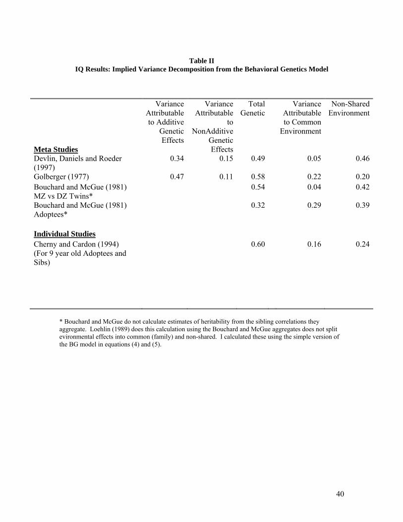
40
Table II
IQ Results: Implied Variance Decomposition from the Behavioral Genetics Model
Meta Studies
Variance Attributable to Additive
Genetic Effects
Variance Attributable
to NonAdditive
Genetic Effects
Total Genetic
Variance Attributable to Common
Environment
Non-Shared Environment
Devlin, Daniels and Roeder (1997)
0.34 0.15 0.49 0.05 0.46
Golberger (1977) 0.47 0.11 0.58 0.22 0.20Bouchard and McGue (1981) MZ vs DZ Twins*
0.54 0.04 0.42
Bouchard and McGue (1981) Adoptees*
0.32 0.29 0.39
Individual Studies Cherny and Cardon (1994) (For 9 year old Adoptees and Sibs)
0.60 0.16 0.24
* Bouchard and McGue do not calculate estimates of heritability from the sibling correlations they aggregate. Loehlin (1989) does this calculation using the Bouchard and McGue aggregates does not split evironmental effects into common (family) and non-shared. I calculated these using the simple version of the BG model in equations (4) and (5).

41
Table III
Years of Education: Implied Variance Decomposition from the Behavioral Genetics Model
Authors and Sample Variance Attributable to Additive
Genetic Effects
Variance Attributable
to NonAdditive
Genetic Effects
Total Genetic
Variance Attributable to Common
Environment
Non-Shared Environment
Behrman and Taubman (1989) 2,000 twins pairs and their relatives NAS-NRC sample
0.88(.002)
-0.01(.047)
0.88
Scarr and Weinberg (1994) 59 adoptive sibling pairs and 105 nonadoptive sibling pairs
0.38 0.13 0.49
Teasdale and Owen (1984) 163 pairs of adoptees from Danish National Register
0.678 0.678 0.052 0.270
Behrman, Taubman, and Wales (1975) 2,478 MZ and DZ Twins in the NAS-NRC sample
0.36 0.41 0.23
Scarr and Weinberg (1994) report adoptive and biological sibling correlations. I used equations (4) and (5) to translate this into the decomposition implied by the simplest form of the BG model. Teasdale and Owen report their results in variance of years of education explained by additive genes, common environment and separate environment. I calculated the fractions explained by each factor. The NAS-NRC sample is a National Academy of Science - National Research Council survey of twins performed in 1974.

42
Table IV Earnings: Implied Variance Decomposition from the Behavioral Genetics Model
Authors and Sample Variance
Attributable Genetic Effects
Variance Attributable to Common
Environment
Variance Attributable
toNon-Shared
Environment
Björklund, Jäntti and Solon (2005) Model 1 Swedish Brothers Including Raised Apart, Together, Twins, Adoptees, Half Sibs
.281(.080)
0.038(0.037)
0.681
Björklund, Jäntti and Solon (2005) Model 1 Swedish Sisters Including Raised Apart, Together, Twins, Adoptees, Half Sibs
.245(.080)
0.009(0.037)
0.746
Björklund, Jäntti and Solon (2005) Model 4 Swedish Brothers Including Raised Apart, Together, Twins, Adoptees, Half Sibs
0.199(0.157)
0.164(0.158)
0.637
Behrman, Taubman, and Wales (1975)
0.45 0.13 -0.42
Björklund, Jäntti and Solon estimates the BG parameters to fit the nine sibling correlations in the data from nine sibling types (MZ raised together, MZ apart, DZ together, DZ apart, Full sibs together, full sibs apart, half sibs together, half sibs apart, adoptive sibs). The difference between models 1 and 4 is that model 4 adds parameters to allow for different degrees of environmental correlation among different types of sibling pairs.

43
Table V Behavioral Genetics Results on Personality Traits
Meta Study of Correlations Between Parents and Children
Parent Child Relationship Biological Social, not Biological, and social biological not social Dimension Extraversion 0.14 0.03 0.16 (117, .010) (40, .011) (15, .019) Agreeableness 0.11 0.01 0.14 (65, .013) (16, .021) (3, .067) Conscientiousness 0.09 0.02 0.11 (64, .013) (26, .012) (2, .110) Neuroticism 0.13 0.05 0.11 (131, .010) (40, .011) (21, .022) Openness 0.17 0.07 0.14 (24, .028) (12, .031) (1 - )
This is a summary of the literature on personality traits and is reprinted exactly from Loehlin (2005) Table 6.3. Number of correlations that were averaged and the implied standard errors are in parentheses.
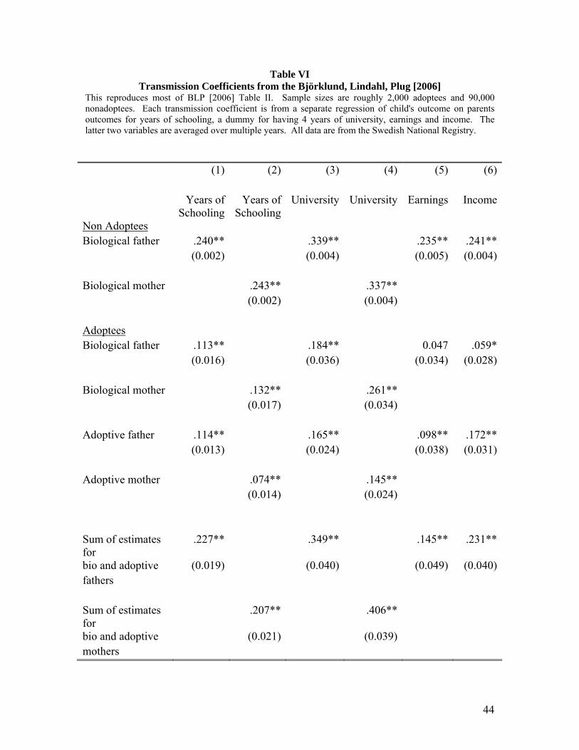
44
Table VI Transmission Coefficients from the Björklund, Lindahl, Plug [2006]
This reproduces most of BLP [2006] Table II. Sample sizes are roughly 2,000 adoptees and 90,000 nonadoptees. Each transmission coefficient is from a separate regression of child's outcome on parents outcomes for years of schooling, a dummy for having 4 years of university, earnings and income. The latter two variables are averaged over multiple years. All data are from the Swedish National Registry. (1) (2) (3) (4) (5) (6)
Years of Schooling
Years of Schooling
University University Earnings Income
Non Adoptees Biological father .240** .339** .235** .241** (0.002) (0.004) (0.005) (0.004) Biological mother .243** .337** (0.002) (0.004) Adoptees Biological father .113** .184** 0.047 .059* (0.016) (0.036) (0.034) (0.028) Biological mother .132** .261** (0.017) (0.034) Adoptive father .114** .165** .098** .172** (0.013) (0.024) (0.038) (0.031) Adoptive mother .074** .145** (0.014) (0.024) Sum of estimates for
.227** .349** .145** .231**
bio and adoptive (0.019) (0.040) (0.049) (0.040)fathers Sum of estimates for
.207** .406**
bio and adoptive (0.021) (0.039) mothers
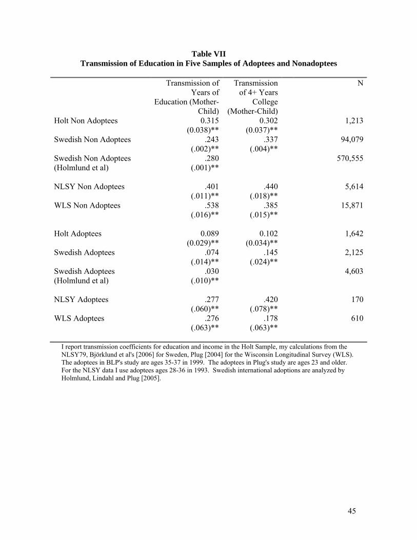
45
Table VII Transmission of Education in Five Samples of Adoptees and Nonadoptees
Transmission of
Years of Education (Mother-
Child)
Transmission of 4+ Years
College (Mother-Child)
N
Holt Non Adoptees 0.315 0.302 1,213 (0.038)** (0.037)**Swedish Non Adoptees .243 .337 94,079 (.002)** (.004)**Swedish Non Adoptees .280 570,555(Holmlund et al)
(.001)**
NLSY Non Adoptees .401 .440 5,614 (.011)** (.018)**WLS Non Adoptees .538 .385 15,871 (.016)** (.015)** Holt Adoptees 0.089 0.102 1,642 (0.029)** (0.034)**Swedish Adoptees .074 .145 2,125 (.014)** (.024)**Swedish Adoptees .030 4,603(Holmlund et al)
(.010)**
NLSY Adoptees .277 .420 170 (.060)** (.078)**WLS Adoptees .276 .178 610 (.063)** (.063)**
I report transmission coefficients for education and income in the Holt Sample, my calculations from the NLSY79, Björklund et al's [2006] for Sweden, Plug [2004] for the Wisconsin Longitudinal Survey (WLS). The adoptees in BLP's study are ages 35-37 in 1999. The adoptees in Plug's study are ages 23 and older. For the NLSY data I use adoptees ages 28-36 in 1993. Swedish international adoptions are analyzed by Holmlund, Lindahl and Plug [2005].
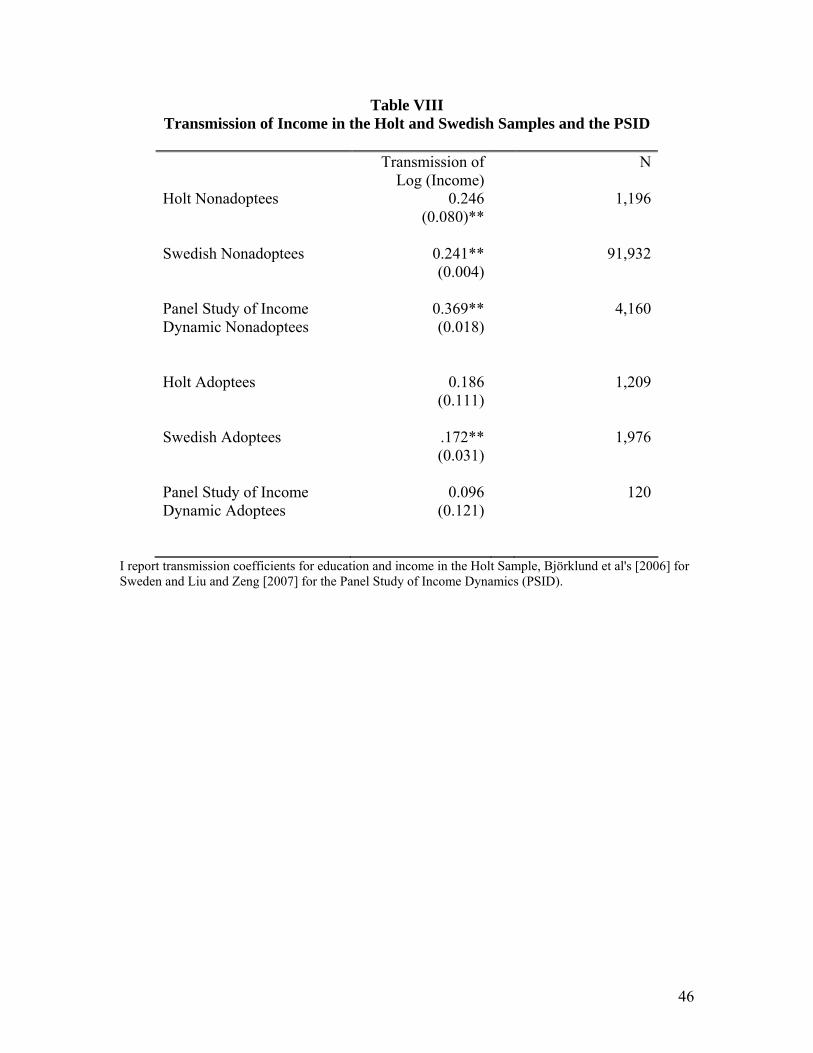
46
Table VIII Transmission of Income in the Holt and Swedish Samples and the PSID
Transmission of
Log (Income)N
Holt Nonadoptees 0.246 1,196
(0.080)**
Swedish Nonadoptees 0.241** 91,932
(0.004)
Panel Study of Income 0.369** 4,160 Dynamic Nonadoptees
(0.018)
Holt Adoptees 0.186 1,209
(0.111)
Swedish Adoptees .172** 1,976
(0.031)
Panel Study of Income 0.096 120 Dynamic Adoptees
(0.121)
I report transmission coefficients for education and income in the Holt Sample, Björklund et al's [2006] for Sweden and Liu and Zeng [2007] for the Panel Study of Income Dynamics (PSID).
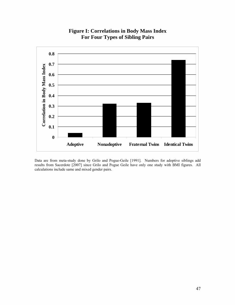
47
Figure I: Correlations in Body Mass Index For Four Types of Sibling Pairs
0
0.1
0.2
0.3
0.4
0.5
0.6
0.7
0.8
Adoptive Nonadoptive Fraternal Twins Identical Twins
Cor
rela
tion
in B
ody
Mas
s Ind
ex
Data are from meta-study done by Grilo and Pogue-Geile [1991]. Numbers for adoptive siblings add results from Sacerdote [2007] since Grilo and Pogue Geile have only one study with BMI figures. All calculations include same and mixed gender pairs.

48
Figure I: Comparison of Coefficient of Transmission from Parent to Child
Reproduced from Sacerdote [2007]. Graph shows coefficient from a regression of child's outcome on mother's outcome for adoptees and nonadoptees in the sample.
Years of EducationHas 4+ Years College
Log Household Income
Height Inches
Is Obese
Is Overweight
BMI
Smokes (0-1)
Drinks (0-1)
0.1
.2.3
.4.5
Non
adop
tees
Tra
nsm
issi
on C
oeff
icie
nt
0 .1 .2 .3 .4 .5Adoptees Transmission Coefficient