natural language processing (almost) from scratch - arxiv · pdf filenatural language...

arXiv

arXiv

Natural Language Processing (almost) from Scratch

Ronan Collobert [email protected]

NEC Labs America, Princeton NJ.

Jason Weston [email protected]

Google, New York, NY.

Leon Bottou [email protected]

Michael Karlen [email protected]

Koray Kavukcuoglu† [email protected]

Pavel Kuksa‡ [email protected]

NEC Labs America, Princeton NJ.

Abstract

We propose a unified neural network architecture and learning algorithm that can be appliedto various natural language processing tasks including: part-of-speech tagging, chunking,named entity recognition, and semantic role labeling. This versatility is achieved by tryingto avoid task-specific engineering and therefore disregarding a lot of prior knowledge.Instead of exploiting man-made input features carefully optimized for each task, our systemlearns internal representations on the basis of vast amounts of mostly unlabeled trainingdata. This work is then used as a basis for building a freely available tagging system withgood performance and minimal computational requirements.

Keywords: Natural Language Processing, Neural Networks

1. Introduction

Will a computer program ever be able to convert a piece of English text into a data structurethat unambiguously and completely describes the meaning of the natural language text?Among numerous problems, no consensus has emerged about the form of such a datastructure. Until such fundamental Artificial Intelligence problems are resolved, computerscientists must settle for reduced objectives: extracting simpler representations describingrestricted aspects of the textual information.

These simpler representations are often motivated by specific applications, for instance,bag-of-words variants for information retrieval. These representations can also be motivatedby our belief that they capture something more general about natural language. Theycan describe syntactic information (e.g. part-of-speech tagging, chunking, and parsing) orsemantic information (e.g. word-sense disambiguation, semantic role labeling, named entityextraction, and anaphora resolution). Text corpora have been manually annotated with suchdata structures in order to compare the performance of various systems. The availability ofstandard benchmarks has stimulated research in Natural Language Processing (NLP) and

†. Koray Kavukcuoglu is also with New York University, New York, NY.‡. Pavel Kuksa is also with Rutgers University, New Brunswick, NJ.

c©2009 Ronan Collobert, Jason Weston, Leon Bottou, Michael Karlen, Koray Kavukcuoglu and Pavel Kuksa.

arX

iv:1

103.

0398

v1 [

cs.L

G]

2 M

ar 2

011

arXiv

Collobert, Weston, Bottou, Karlen, Kavukcuoglu and Kuksa

effective systems have been designed for all these tasks. Such systems are often viewed assoftware components for constructing real-world NLP solutions.

The overwhelming majority of these state-of-the-art systems address a benchmarktask by applying linear statistical models to ad-hoc features. In other words, theresearchers themselves discover intermediate representations by engineering task-specificfeatures. These features are often derived from the output of preexisting systems, leadingto complex runtime dependencies. This approach is effective because researchers leveragea large body of linguistic knowledge. On the other hand, there is a great temptation tooptimize the performance of a system for a specific benchmark. Although such performanceimprovements can be very useful in practice, they teach us little about the means to progresstoward the broader goals of natural language understanding and the elusive goals of ArtificialIntelligence.

In this contribution, we try to excel on multiple benchmarks while avoiding task-specificenginering. Instead we use a single learning system able to discover adequate internalrepresentations. In fact we view the benchmarks as indirect measurements of the relevanceof the internal representations discovered by the learning procedure, and we posit that theseintermediate representations are more general than any of the benchmarks. Our desire toavoid task-specific engineered features led us to ignore a large body of linguistic knowledge.Instead we reach good performance levels in most of the tasks by transferring intermediaterepresentations discovered on large unlabeled datasets. We call this approach “almost fromscratch” to emphasize the reduced (but still important) reliance on a priori NLP knowledge.

The paper is organized as follows. Section 2 describes the benchmark tasks ofinterest. Section 3 describes the unified model and reports benchmark results obtained withsupervised training. Section 4 leverages large unlabeled datasets (∼ 852 million words)to train the model on a language modeling task. Performance improvements are thendemonstrated by transferring the unsupervised internal representations into the supervisedbenchmark models. Section 5 investigates multitask supervised training. Section 6 thenevaluates how much further improvement can be achieved by incorporating standard NLPtask-specific engineering into our systems. Drifting away from our initial goals gives us theopportunity to construct an all-purpose tagger that is simultaneously accurate, practical,and fast. We then conclude with a short discussion section.

2. The Benchmark Tasks

In this section, we briefly introduce four standard NLP tasks on which we will benchmarkour architectures within this paper: Part-Of-Speech tagging (POS), chunking (CHUNK),Named Entity Recognition (NER) and Semantic Role Labeling (SRL). For each of them,we consider a standard experimental setup and give an overview of state-of-the-art systemson this setup. The experimental setups are summarized in Table 1, while state-of-the-artsystems are reported in Table 2.

2.1 Part-Of-Speech Tagging

POS aims at labeling each word with a unique tag that indicates its syntactic role, e.g.plural noun, adverb, . . . A standard benchmark setup is described in detail by Toutanova

2

arXiv


Task Benchmark Dataset Training set Test set(#tokens) (#tokens) (#tags)

POS Toutanova et al. (2003) WSJ sections 0–18 sections 22–24 ( 45 )( 912,344 ) ( 129,654 )

Chunking CoNLL 2000 WSJ sections 15–18 section 20 ( 42 )( 211,727 ) ( 47,377 ) (IOBES)

NER CoNLL 2003 Reuters “eng.train” “eng.testb” ( 17 )( 203,621 ) ( 46,435 ) (IOBES)

SRL CoNLL 2005 WSJ sections 2–21 section 23 ( 186 )( 950,028 ) + 3 Brown sections (IOBES)

( 63,843 )

Table 1: Experimental setup: for each task, we report the standard benchmark we used,the dataset it relates to, as well as training and test information.

System Accuracy

Shen et al. (2007) 97.33%Toutanova et al. (2003) 97.24%Gimenez and Marquez (2004) 97.16%

(a) POS

System F1

Shen and Sarkar (2005) 95.23%Sha and Pereira (2003) 94.29%Kudo and Matsumoto (2001) 93.91%

(b) CHUNK

System F1

Ando and Zhang (2005) 89.31%Florian et al. (2003) 88.76%Kudo and Matsumoto (2001) 88.31%

(c) NER

System F1

Koomen et al. (2005) 77.92%Pradhan et al. (2005) 77.30%Haghighi et al. (2005) 77.04%

(d) SRL

Table 2: State-of-the-art systems on four NLP tasks. Performance is reported in per-wordaccuracy for POS, and F1 score for CHUNK, NER and SRL. Systems in bold will be referredas benchmark systems in the rest of the paper (see text).

et al. (2003). Sections 0–18 of Wall Street Journal (WSJ) data are used for training, whilesections 19–21 are for validation and sections 22–24 for testing.

The best POS classifiers are based on classifiers trained on windows of text, which arethen fed to a bidirectional decoding algorithm during inference. Features include precedingand following tag context as well as multiple words (bigrams, trigrams. . . ) context, andhandcrafted features to deal with unknown words. Toutanova et al. (2003), who usemaximum entropy classifiers, and a bidirectional dependency network (Heckerman et al.,2001) at inference, reach 97.24% per-word accuracy. Gimenez and Marquez (2004) proposeda SVM approach also trained on text windows, with bidirectional inference achieved withtwo Viterbi decoders (left-to-right and right-to-left). They obtained 97.16% per-wordaccuracy. More recently, Shen et al. (2007) pushed the state-of-the-art up to 97.33%,with a new learning algorithm they call guided learning, also for bidirectional sequenceclassification.

3

arXiv


2.2 Chunking

Also called shallow parsing, chunking aims at labeling segments of a sentence with syntacticconstituents such as noun or verb phrases (NP or VP). Each word is assigned only one uniquetag, often encoded as a begin-chunk (e.g. B-NP) or inside-chunk tag (e.g. I-NP). Chunkingis often evaluated using the CoNLL 2000 shared task1. Sections 15–18 of WSJ data areused for training and section 20 for testing. Validation is achieved by splitting the trainingset.

Kudoh and Matsumoto (2000) won the CoNLL 2000 challenge on chunking with a F1-score of 93.48%. Their system was based on Support Vector Machines (SVMs). EachSVM was trained in a pairwise classification manner, and fed with a window around theword of interest containing POS and words as features, as well as surrounding tags. Theyperform dynamic programming at test time. Later, they improved their results up to93.91% (Kudo and Matsumoto, 2001) using an ensemble of classifiers trained with differenttagging conventions (see Section 3.2.3).

Since then, a certain number of systems based on second-order random fields werereported (Sha and Pereira, 2003; McDonald et al., 2005; Sun et al., 2008), all reportingaround 94.3% F1 score. These systems use features composed of words, POS tags, andtags.

More recently, Shen and Sarkar (2005) obtained 95.23% using a voting classifier scheme,where each classifier is trained on different tag representations2 (IOB, IOE, . . . ). They usePOS features coming from an external tagger, as well carefully hand-crafted specializationfeatures which again change the data representation by concatenating some (carefullychosen) chunk tags or some words with their POS representation. They then build trigramsover these features, which are finally passed through a Viterbi decoder a test time.

2.3 Named Entity Recognition

NER labels atomic elements in the sentence into categories such as “PERSON” or“LOCATION”. As in the chunking task, each word is assigned a tag prefixed by an indicatorof the beginning or the inside of an entity. The CoNLL 2003 setup3 is a NER benchmarkdataset based on Reuters data. The contest provides training, validation and testing sets.

Florian et al. (2003) presented the best system at the NER CoNLL 2003 challenge, with88.76% F1 score. They used a combination of various machine-learning classifiers. Featuresthey picked included words, POS tags, CHUNK tags, prefixes and suffixes, a large gazetteer(not provided by the challenge), as well as the output of two other NER classifiers trainedon richer datasets. Chieu (2003), the second best performer of CoNLL 2003 (88.31% F1),also used an external gazetteer (their performance goes down to 86.84% with no gazetteer)and several hand-chosen features.

Later, Ando and Zhang (2005) reached 89.31% F1 with a semi-supervised approach.They trained jointly a linear model on NER with a linear model on two auxiliaryunsupervised tasks. They also performed Viterbi decoding at test time. The unlabeled

1. See http://www.cnts.ua.ac.be/conll2000/chunking.2. See Table 3 for tagging scheme details.3. See http://www.cnts.ua.ac.be/conll2003/ner.

4

http://www.cnts.ua.ac.be/conll2000/chunking

http://www.cnts.ua.ac.be/conll2003/ner

arXiv


corpus was 27M words taken from Reuters. Features included words, POS tags, suffixesand prefixes or CHUNK tags, but overall were less specialized than CoNLL 2003 challengers.

2.4 Semantic Role Labeling

SRL aims at giving a semantic role to a syntactic constituent of a sentence. In thePropBank (Palmer et al., 2005) formalism one assigns roles ARG0-5 to words that arearguments of a verb (or more technically, a predicate) in the sentence, e.g. the followingsentence might be tagged “[John]ARG0 [ate]REL [the apple]ARG1 ”, where “ate” is thepredicate. The precise arguments depend on a verb’s frame and if there are multiple verbsin a sentence some words might have multiple tags. In addition to the ARG0-5 tags,there there are several modifier tags such as ARGM-LOC (locational) and ARGM-TMP(temporal) that operate in a similar way for all verbs. We picked CoNLL 20054 as our SRLbenchmark. It takes sections 2–21 of WSJ data as training set, and section 24 as validationset. A test set composed of section 23 of WSJ concatenated with 3 sections from the Browncorpus is also provided by the challenge.

State-of-the-art SRL systems consist of several stages: producing a parse tree, identifyingwhich parse tree nodes represent the arguments of a given verb, and finally classifying thesenodes to compute the corresponding SRL tags. This entails extracting numerous basefeatures from the parse tree and feeding them into statistical models. Feature categoriescommonly used by these system include (Gildea and Jurafsky, 2002; Pradhan et al., 2004):

• the parts of speech and syntactic labels of words and nodes in the tree;

• the node’s position (left or right) in relation to the verb;

• the syntactic path to the verb in the parse tree;

• whether a node in the parse tree is part of a noun or verb phrase;

• the voice of the sentence: active or passive;

• the node’s head word; and

• the verb sub-categorization.

Pradhan et al. (2004) take these base features and define additional features, notablythe part-of-speech tag of the head word, the predicted named entity class of the argument,features providing word sense disambiguation for the verb (they add 25 variants of 12 newfeature types overall). This system is close to the state-of-the-art in performance. Pradhanet al. (2005) obtain 77.30% F1 with a system based on SVM classifiers and simultaneouslyusing the two parse trees provided for the SRL task. In the same spirit, Haghighi et al.(2005) use log-linear models on each tree node, re-ranked globally with a dynamic algorithm.Their system reaches 77.04% using the five top Charniak parse trees.

Koomen et al. (2005) hold the state-of-the-art with Winnow-like (Littlestone, 1988)classifiers, followed by a decoding stage based on an integer program that enforces specificconstraints on SRL tags. They reach 77.92% F1 on CoNLL 2005, thanks to the five topparse trees produced by the Charniak (2000) parser (only the first one was provided by thecontest) as well as the Collins (1999) parse tree.

4. See http://www.lsi.upc.edu/~srlconll.

5

http://www.lsi.upc.edu/~srlconll

arXiv


2.5 Evaluation

In our experiments, we strictly followed the standard evaluation procedure of each CoNLLchallenges for NER, CHUNK and SRL. All these three tasks are evaluated by computing theF1 scores over chunks produced by our models. The POS task is evaluated by computingthe per-word accuracy, as it is the case for the standard benchmark we refer to (Toutanovaet al., 2003). We picked the conlleval script5 for evaluating POS6, NER and CHUNK.For SRL, we used the srl-eval.pl script included in the srlconll package7.

2.6 Discussion

When participating in an (open) challenge, it is legitimate to increase generalization by allmeans. It is thus not surprising to see many top CoNLL systems using external labeled data,like additional NER classifiers for the NER architecture of Florian et al. (2003) or additionalparse trees for SRL systems (Koomen et al., 2005). Combining multiple systems or tweakingcarefully features is also a common approach, like in the chunking top system (Shen andSarkar, 2005).

However, when comparing systems, we do not learn anything of the quality of eachsystem if they were trained with different labeled data. For that reason, we will refer tobenchmark systems, that is, top existing systems which avoid usage of external data andhave been well-established in the NLP field: (Toutanova et al., 2003) for POS and (Sha andPereira, 2003) for chunking. For NER we consider (Ando and Zhang, 2005) as they wereusing additional unlabeled data only. We picked (Koomen et al., 2005) for SRL, keeping inmind they use 4 additional parse trees not provided by the challenge. These benchmarksystems will serve as baseline references in our experiments. We marked them in boldin Table 2.

We note that for the four tasks we are considering in this work, it can be seen that for themore complex tasks (with corresponding lower accuracies), the best systems proposed havemore engineered features relative to the best systems on the simpler tasks. That is, the POStask is one of the simplest of our four tasks, and only has relatively few engineered features,whereas SRL is the most complex, and many kinds of features have been designed for it.This clearly has implications for as yet unsolved NLP tasks requiring more sophisticatedsemantic understanding than the ones considered here.

3. The Networks

All the NLP tasks above can be seen as tasks assigning labels to words. The traditional NLPapproach is: extract from the sentence a rich set of hand-designed features which are thenfed to a standard classification algorithm, e.g. a Support Vector Machine (SVM), often witha linear kernel. The choice of features is a completely empirical process, mainly based firston linguistic intuition, and then trial and error, and the feature selection is task dependent,implying additional research for each new NLP task. Complex tasks like SRL then requirea large number of possibly complex features (e.g., extracted from a parse tree) which can

5. Available at http://www.cnts.ua.ac.be/conll2000/chunking/conlleval.txt.6. We used the “-r” option of the conlleval script to get the per-word accuracy, for POS only.7. Available at http://www.lsi.upc.es/~srlconll/srlconll-1.1.tgz.

6

http://www.cnts.ua.ac.be/conll2000/chunking/conlleval.txt

http://www.lsi.upc.es/~srlconll/srlconll-1.1.tgz

arXiv


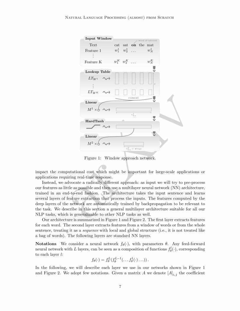
Input Window

Lookup Table

Linear

HardTanh

Linear

Text cat sat on the mat

Feature 1 w11 w1

2 . . . w1N

...

Feature K wK1 wK

2 . . . wKN

LTW 1

...

LTWK

M1 × ·

M2 × ·

word of interest

d

concat

n1hu

n2hu = #tags

Figure 1: Window approach network.

impact the computational cost which might be important for large-scale applications orapplications requiring real-time response.

Instead, we advocate a radically different approach: as input we will try to pre-processour features as little as possible and then use a multilayer neural network (NN) architecture,trained in an end-to-end fashion. The architecture takes the input sentence and learnsseveral layers of feature extraction that process the inputs. The features computed by thedeep layers of the network are automatically trained by backpropagation to be relevant tothe task. We describe in this section a general multilayer architecture suitable for all ourNLP tasks, which is generalizable to other NLP tasks as well.

Our architecture is summarized in Figure 1 and Figure 2. The first layer extracts featuresfor each word. The second layer extracts features from a window of words or from the wholesentence, treating it as a sequence with local and global structure (i.e., it is not treated likea bag of words). The following layers are standard NN layers.

Notations We consider a neural network fθ(·), with parameters θ. Any feed-forwardneural network with L layers, can be seen as a composition of functions f lθ(·), correspondingto each layer l:

fθ(·) = fLθ (fL−1θ (. . . f1

θ (·) . . .)) .In the following, we will describe each layer we use in our networks shown in Figure 1and Figure 2. We adopt few notations. Given a matrix A we denote [A]i, j the coefficient

7

arXiv


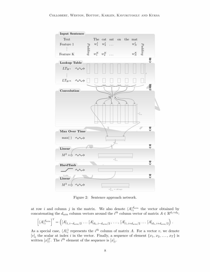
Input Sentence

Lookup Table

Convolution

Max Over Time

Linear

HardTanh

Linear

Text The cat sat on the mat

Feature 1 w11 w1

2 . . . w1N

...

Feature K wK1 wK

2 . . . wKN

LTW 1

...

LTWK

max(·)

M2 × ·

M3 × ·

d

Padding

Padding

n1hu

M1 × ·

n1hu

n2hu

n3hu = #tags

Figure 2: Sentence approach network.

at row i and column j in the matrix. We also denote 〈A〉dwini the vector obtained byconcatenating the dwin column vectors around the ith column vector of matrix A ∈ Rd1×d2 :[

〈A〉dwini

]T=(

[A]1, i−dwin/2 . . . [A]d1, i−dwin/2 , . . . , [A]1, i+dwin/2 . . . [A]d1, i+dwin/2

).

As a special case, 〈A〉1i represents the ith column of matrix A. For a vector v, we denote[v]i the scalar at index i in the vector. Finally, a sequence of element {x1, x2, . . . , xT } iswritten [x]T1 . The ith element of the sequence is [x]i.

8

arXiv


3.1 Transforming Words into Feature Vectors

One of the essential key points of our architecture is its ability to perform well with theuse of (almost8) raw words. The ability for our method to learn good word representationsis thus crucial to our approach. For efficiency, words are fed to our architecture as indicestaken from a finite dictionary D. Obviously, a simple index does not carry much usefulinformation about the word. However, the first layer of our network maps each of theseword indices into a feature vector, by a lookup table operation. Given a task of interest, arelevant representation of each word is then given by the corresponding lookup table featurevector, which is trained by backpropagation.

More formally, for each word w ∈ D, an internal dwrd-dimensional feature vectorrepresentation is given by the lookup table layer LTW (·):

LTW (w) = 〈W 〉1w ,

where W ∈ Rdwrd×|D| is a matrix of parameters to be learnt, 〈W 〉1w ∈ Rdwrd is the wth

column of W and dwrd is the word vector size (a hyper-parameter to be chosen by the user).Given a sentence or any sequence of T words [w]T1 in D, the lookup table layer applies thesame operation for each word in the sequence, producing the following output matrix:

LTW ([w]T1 ) =(〈W 〉1[w]1

〈W 〉1[w]2. . . 〈W 〉1[w]T

). (1)

This matrix can then be fed to further neural network layers, as we will see below.

3.1.1 Extending to Any Discrete Features

One might want to provide features other than words if one suspects that these features arehelpful for the task of interest. For example, for the NER task, one could provide a featurewhich says if a word is in a gazetteer or not. Another common practice is to introduce somebasic pre-processing, such as word-stemming or dealing with upper and lower case. In thislatter option, the word would be then represented by three discrete features: its lower casestemmed root, its lower case ending, and a capitalization feature.

Generally speaking, we can consider a word as represented by K discrete features w ∈D1×· · ·×DK , where Dk is the dictionary for the kth feature. We associate to each feature alookup table LTWk(·), with parameters W k ∈ Rdkwrd×|Dk| where dkwrd ∈ N is a user-specifiedvector size. Given a word w, a feature vector of dimension dwrd =

∑k d

kwrd is then obtained

by concatenating all lookup table outputs:

LTW 1,...,WK (w) =

LTW 1(w1)...

LTWK (wK)

=

〈W 1〉1w1...

〈WK〉1wK

.

8. We did some pre-processing, namely lowercasing and encoding capitalization as another feature. Withenough (unlabeled) training data, presumably we could learn a model without this processing. Ideally,an even more raw input would be to learn from letter sequences rather than words, however we felt thatthis was beyond the scope of this work.

9

arXiv


The matrix output of the lookup table layer for a sequence of words [w]T1 is then similarto (1), but where extra rows have been added for each discrete feature:

LTW 1,...,WK ([w]T1 ) =

〈W 1〉1[w1]1

. . . 〈W 1〉1[w1]T...

...〈WK〉1[wK ]1

. . . 〈WK〉1[wK ]T

. (2)

These vector features in the lookup table effectively learn features for words in the dictionary.Now, we want to use these trainable features as input to further layers of trainable featureextractors, that can represent groups of words and then finally sentences.

3.2 Extracting Higher Level Features from Word Feature Vectors

Feature vectors produced by the lookup table layer need to be combined in subsequent layersof the neural network to produce a tag decision for each word in the sentence. Producingtags for each element in variable length sequences (here, a sentence is a sequence of words)is a standard problem in machine-learning. We consider two common approaches which tagone word at the time: a window approach, and a (convolutional) sentence approach.

3.2.1 Window Approach

A window approach assumes the tag of a word depends mainly on its neighboring words.Given a word to tag, we consider a fixed size ksz (a hyper-parameter) window of wordsaround this word. Each word in the window is first passed through the lookup table layer (1)or (2), producing a matrix of word features of fixed size dwrd × ksz. This matrix can beviewed as a dwrd ksz-dimensional vector by concatenating each column vector, which can befed to further neural network layers. More formally, the word feature window given by thefirst network layer can be written as:

f1θ = 〈LTW ([w]T1 )〉dwint =

〈W 〉1[w]t−dwin/2...

〈W 〉1[w]t...

〈W 〉1[w]t+dwin/2

. (3)

Linear Layer The fixed size vector f1θ can be fed to one or several standard neural

network layers which perform affine transformations over their inputs:

f lθ = W l f l−1θ + bl , (4)

where W l ∈ Rnlhu×nl−1hu and bl ∈ Rnlhu are the parameters to be trained. The hyper-parameter

nlhu is usually called the number of hidden units of the lth layer.

HardTanh Layer Several linear layers are often stacked, interleaved with a non-linearityfunction, to extract highly non-linear features. If no non-linearity is introduced, our network

10

arXiv


would be a simple linear model. We chose a “hard” version of the hyperbolic tangent as non-linearity. It has the advantage of being slightly cheaper to compute (compared to the exacthyperbolic tangent), while leaving the generalization performance unchanged (Collobert,2004). The corresponding layer l applies a HardTanh over its input vector:[

f lθ

]i

= HardTanh([f l−1θ

]i) ,

where

HardTanh(x) =

−1 if x < −1x if − 1 <= x <= 11 if x > 1

. (5)

Scoring Finally, the output size of the last layer L of our network is equal to the numberof possible tags for the task of interest. Each output can be then interpreted as a score ofthe corresponding tag (given the input of the network), thanks to a carefully chosen costfunction that we will describe later in this section.

Remark 1 (Border Effects) The feature window (3) is not well defined for words nearthe beginning or the end of a sentence. To circumvent this problem, we augment the sentencewith a special “PADDING” word replicated dwin/2 times at the beginning and the end. Thisis akin to the use of “start” and “stop” symbols in sequence models.

3.2.2 Sentence Approach

We will see in the experimental section that a window approach performs well for mostnatural language processing tasks we are interested in. However this approach fails withSRL, where the tag of a word depends on a verb (or, more correctly, predicate) chosenbeforehand in the sentence. If the verb falls outside the window, one cannot expect this wordto be tagged correctly. In this particular case, tagging a word requires the consideration ofthe whole sentence. When using neural networks, the natural choice to tackle this problembecomes a convolutional approach, first introduced by Waibel et al. (1989) and also calledTime Delay Neural Networks (TDNNs) in the literature.

We describe in detail our convolutional network below. It successively takes the completesentence, passes it through the lookup table layer (1), produces local features around eachword of the sentence thanks to convolutional layers, combines these feature into a globalfeature vector which can then be fed to standard affine layers (4). In the semantic rolelabeling case, this operation is performed for each word in the sentence, and for each verbin the sentence. It is thus necessary to encode in the network architecture which verb weare considering in the sentence, and which word we want to tag. For that purpose, eachword at position i in the sentence is augmented with two features in the way describedin Section 3.1.1. These features encode the relative distances i − posv and i − posw withrespect to the chosen verb at position posv, and the word to tag at position posw respectively.

Convolutional Layer A convolutional layer can be seen as a generalization of a windowapproach: given a sequence represented by columns in a matrix f l−1

θ (in our lookup tablematrix (1)), a matrix-vector operation as in (4) is applied to each window of successive

11

arXiv


0

10

20

30

40

50

60

70

Theproposed

changes

alsowould

allowexecutives

to report

exercises

of options

laterand

lessoften

. 0

10

20

30

40

50

60

70

Theproposed

changes

alsowould

allowexecutives

to report

exercises

of options

laterand

lessoften

.

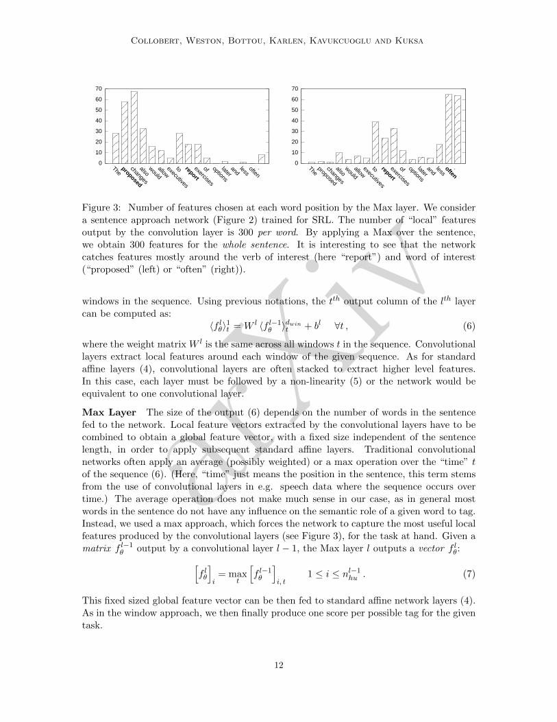
Figure 3: Number of features chosen at each word position by the Max layer. We considera sentence approach network (Figure 2) trained for SRL. The number of “local” featuresoutput by the convolution layer is 300 per word. By applying a Max over the sentence,we obtain 300 features for the whole sentence. It is interesting to see that the networkcatches features mostly around the verb of interest (here “report”) and word of interest(“proposed” (left) or “often” (right)).

windows in the sequence. Using previous notations, the tth output column of the lth layercan be computed as:

〈f lθ〉1t = W l 〈f l−1θ 〉dwint + bl ∀t , (6)

where the weight matrix W l is the same across all windows t in the sequence. Convolutionallayers extract local features around each window of the given sequence. As for standardaffine layers (4), convolutional layers are often stacked to extract higher level features.In this case, each layer must be followed by a non-linearity (5) or the network would beequivalent to one convolutional layer.

Max Layer The size of the output (6) depends on the number of words in the sentencefed to the network. Local feature vectors extracted by the convolutional layers have to becombined to obtain a global feature vector, with a fixed size independent of the sentencelength, in order to apply subsequent standard affine layers. Traditional convolutionalnetworks often apply an average (possibly weighted) or a max operation over the “time” tof the sequence (6). (Here, “time” just means the position in the sentence, this term stemsfrom the use of convolutional layers in e.g. speech data where the sequence occurs overtime.) The average operation does not make much sense in our case, as in general mostwords in the sentence do not have any influence on the semantic role of a given word to tag.Instead, we used a max approach, which forces the network to capture the most useful localfeatures produced by the convolutional layers (see Figure 3), for the task at hand. Given amatrix f l−1

θ output by a convolutional layer l − 1, the Max layer l outputs a vector f lθ:[f lθ

]i

= maxt

[f l−1θ

]i, t

1 ≤ i ≤ nl−1hu . (7)

This fixed sized global feature vector can be then fed to standard affine network layers (4).As in the window approach, we then finally produce one score per possible tag for the giventask.

12

arXiv


Scheme Begin Inside End Single OtherIOB B-X I-X I-X B-X OIOE I-X I-X E-X E-X OIOBES B-X I-X E-X S-X O

Table 3: Various tagging schemes. Each word in a segment labeled “X” is tagged with aprefixed label, depending of the word position in the segment (begin, inside, end). Singleword segment labeling is also output. Words not in a labeled segment are labeled “O”.Variants of the IOB (and IOE) scheme exist, where the prefix B (or E) is replaced by I forall segments not contiguous with another segment having the same label “X”.

Remark 2 The same border effects arise in the convolution operation (6) as in the windowapproach (3). We again work around this problem by padding the sentences with a specialword.

3.2.3 Tagging Schemes

As explained earlier, the network output layers compute scores for all the possible tags forthe task of interest. In the window approach, these tags apply to the word located in thecenter of the window. In the (convolutional) sentence approach, these tags apply to theword designated by additional markers in the network input.

The POS task indeed consists of marking the syntactic role of each word. However, theremaining three tasks associate labels with segments of a sentence. This is usually achievedby using special tagging schemes to identify the segment boundaries, as shown in Table 3.Several such schemes have been defined (IOB, IOE, IOBES, . . . ) without clear conclusionas to which scheme is better in general. State-of-the-art performance is sometimes obtainedby combining classifiers trained with different tagging schemes (e.g. Kudo and Matsumoto,2001).

The ground truth for the NER, CHUNK, and SRL tasks is provided using two differenttagging schemes. In order to eliminate this additional source of variations, we have decidedto use the most expressive IOBES tagging scheme for all tasks. For instance, in the CHUNKtask, we describe noun phrases using four different tags. Tag “S-NP” is used to mark a nounphrase containing a single word. Otherwise tags “B-NP”, “I-NP”, and “E-NP” are usedto mark the first, intermediate and last words of the noun phrase. An additional tag “O”marks words that are not members of a chunk. During testing, these tags are then convertedto the original IOB tagging scheme and fed to the standard performance evaluation scriptsmentioned in Section 2.5.

3.3 Training

All our neural networks are trained by maximizing a likelihood over the training data, usingstochastic gradient ascent. If we denote θ to be all the trainable parameters of the network,which are trained using a training set T we want to maximize the following log-likelihood

13

arXiv


with respect to θ:

θ 7→∑

(x, y)∈T

log p(y |x, θ) , (8)

where x corresponds to either a training word window or a sentence and its associatedfeatures, and y represents the corresponding tag. The probability p(·) is computed from theoutputs of the neural network. We will see in this section two ways of interpreting neuralnetwork outputs as probabilities.

3.3.1 Word-Level Log-Likelihood

In this approach, each word in a sentence is considered independently. Given an inputexample x, the network with parameters θ outputs a score [fθ(x)]i, for the ith tag withrespect to the task of interest. To simplify the notation, we drop x from now, and we writeinstead [fθ]i. This score can be interpreted as a conditional tag probability p(i |x, θ) byapplying a softmax (Bridle, 1990) operation over all the tags:

p(i |x, θ) =e[fθ]i∑j e

[fθ]j. (9)

Defining the log-add operation as

logaddi

zi = log(∑i

ezi) , (10)

we can express the log-likelihood for one training example (x, y) as follows:

log p(y |x, θ) = [fθ]y − logaddj

[fθ]j . (11)

While this training criterion, often referred as cross-entropy is widely used for classificationproblems, it might not be ideal in our case, where there is often a correlation between thetag of a word in a sentence and its neighboring tags. We now describe another commonapproach for neural networks which enforces dependencies between the predicted tags in asentence.

3.3.2 Sentence-Level Log-Likelihood

In tasks like chunking, NER or SRL we know that there are dependencies between wordtags in a sentence: not only are tags organized in chunks, but some tags cannot followother tags. Training using a word-level approach discards this kind of labeling information.We consider a training scheme which takes into account the sentence structure: given thepredictions of all tags by our network for all words in a sentence, and given a score for goingfrom one tag to another tag, we want to encourage valid paths of tags during training, whilediscouraging all other paths.

We consider the matrix of scores fθ([x]T1 ) output by the network. As before, we drop theinput [x]T1 for notation simplification. The element [fθ]i, t of the matrix is the score output

by the network with parameters θ, for the sentence [x]T1 and for the ith tag, at the tth word.

14

arXiv


We introduce a transition score [A]i, j for jumping from i to j tags in successive words, and

an initial score [A]i, 0 for starting from the ith tag. As the transition scores are going to be

trained (as are all network parameters θ), we define θ = θ ∪ {[A]i, j ∀i, j}. The score of

a sentence [x]T1 along a path of tags [i]T1 is then given by the sum of transition scores andnetwork scores:

s([x]T1 , [i]T1 , θ) =T∑t=1

([A][i]t−1, [i]t

+ [fθ][i]t, t

). (12)

Exactly as for the word-level likelihood (11), where we were normalizing with respect to alltags using a softmax (9), we normalize this score over all possible tag paths [j]T1 using asoftmax, and we interpret the resulting ratio as a conditional tag path probability. Takingthe log, the conditional probability of the true path [y]T1 is therefore given by:

log p([y]T1 | [x]T1 , θ) = s([x]T1 , [y]T1 , θ)− logadd∀[j]T1

s([x]T1 , [j]T1 , θ) . (13)

While the number of terms in the logadd operation (11) was equal to the number of tags, itgrows exponentially with the length of the sentence in (13). Fortunately, one can computeit in linear time with the following standard recursion over t, taking advantage of theassociativity and distributivity on the semi-ring9 (R ∪ {−∞}, logadd, +):

δt(k)∆= logadd{[j]t1 ∩ [j]t=k}

s([x]t1, [j]t1, θ)

= logaddi

logadd{[j]t1 ∩ [j]t−1=i∩ [j]t=k}

s([x]t1, [j]t−11 , θ) + [A][j]t−1, k

+ [fθ]k, t

= logaddi

δt−1(i) + [A]i, k + [fθ]k, t

= [fθ]k, t + logaddi

(δt−1(i) + [A]i, k

)∀k ,

(14)

followed by the termination

logadd∀[j]T1

s([x]T1 , [j]T1 , θ) = logaddi

δT (i) . (15)

We can now maximize in (8) the log-likelihood (13) over all the training pairs ([x]T1 , [y]T1 ).At inference time, given a sentence [x]T1 to tag, we have to find the best tag path which

minimizes the sentence score (12). In other words, we must find

argmax[j]T1

s([x]T1 , [j]T1 , θ) . (16)

The Viterbi algorithm is the natural choice for this inference. It corresponds to performingthe recursion (14) and (15), but where the logadd is replaced by a max, and then trackingback the optimal path through each max.

9. In other words, read logadd as ⊕ and + as ⊗.

15

arXiv


Remark 3 (Graph Transformer Networks) Our approach is a particular case of thediscriminative forward training for graph transformer networks (GTNs) (Bottou et al., 1997;Le Cun et al., 1998). The log-likelihood (13) can be viewed as the difference between theforward score constrained over the valid paths (in our case there is only the labeled path)and the unconstrained forward score (15).

Remark 4 (Conditional Random Fields) An important feature of equation (12) is the

absence of normalization. Summing the exponentials e[fθ]i, t over all possible tags does

not necessarily yield the unity. If this was the case, the scores could be viewed as thelogarithms of conditional transition probabilities, and our model would be subject to thelabel-bias problem that motivates Conditional Random Fields (CRFs) (Lafferty et al., 2001).The denormalized scores should instead be likened to the potential functions of a CRF.In fact, a CRF maximizes the same likelihood (13) using a linear model instead of anonlinear neural network. CRFs have been widely used in the NLP world, such as for POStagging (Lafferty et al., 2001), chunking (Sha and Pereira, 2003), NER (McCallum and Li,2003) or SRL (Cohn and Blunsom, 2005). Compared to such CRFs, we take advantage ofthe nonlinear network to learn appropriate features for each task of interest.

3.3.3 Stochastic Gradient

Maximizing (8) with stochastic gradient (Bottou, 1991) is achieved by iteratively selectinga random example (x, y) and making a gradient step:

θ ←− θ + λ∂ log p(y |x, θ)

∂θ, (17)

where λ is a chosen learning rate. Our neural networks described in Figure 1 and Figure 2are a succession of layers that correspond to successive composition of functions. The neuralnetwork is finally composed with the word-level log-likelihood (11), or successively composedin the recursion (14) if using the sentence-level log-likelihood (13). Thus, an analyticalformulation of the derivative (17) can be computed, by applying the differentiation chainrule through the network, and through the word-level log-likelihood (11) or through therecurrence (14).

Remark 5 (Differentiability) Our cost functions are differentiable almost everywhere.Non-differentiable points arise because we use a “hard” transfer function (5) and becausewe use a “max” layer (7) in the sentence approach network. Fortunately, stochasticgradient still converges to a meaningful local minimum despite such minor differentiabilityproblems (Bottou, 1991, 1998). Stochastic gradient iterations that hit a non-differentiabilityare simply skipped.

Remark 6 (Modular Approach) The well known “back-propagation” algorithm (LeCun,1985; Rumelhart et al., 1986) computes gradients using the chain rule. The chain rule canalso be used in a modular implementation.10 Our modules correspond to the boxes in Figure 1and Figure 2. Given derivatives with respect to its outputs, each module can independently

10. See http://torch5.sf.net.

16

http://torch5.sf.net

arXiv


Approach POS Chunking NER SRL(PWA) (F1) (F1) (F1)

Benchmark Systems 97.24 94.29 89.31 77.92

NN+WLL 96.31 89.13 79.53 55.40NN+SLL 96.37 90.33 81.47 70.99

Table 4: Comparison in generalization performance of benchmark NLP systems with avanilla neural network (NN) approach, on POS, chunking, NER and SRL tasks. We reportresults with both the word-level log-likelihood (WLL) and the sentence-level log-likelihood(SLL). Generalization performance is reported in per-word accuracy rate (PWA) for POSand F1 score for other tasks. The NN results are behind the benchmark results, in Section 4we show how to improve these models using unlabeled data.

Task Window/Conv. size Word dim. Caps dim. Hidden units Learning rate

POS dwin = 5 d0 = 50 d1 = 5 n1hu = 300 λ = 0.01

CHUNK ” ” ” ” ”

NER ” ” ” ” ”

SRL ” ” ”n1hu = 300

n2hu = 500

”

Table 5: Hyper-parameters of our networks. We report for each task the window size(or convolution size), word feature dimension, capital feature dimension, number of hiddenunits and learning rate.

compute derivatives with respect to its inputs and with respect to its trainable parameters,as proposed by Bottou and Gallinari (1991). This allows us to easily build variants of ournetworks. For details about gradient computations, see Appendix A.

Remark 7 (Tricks) Many tricks have been reported for training neural networks (LeCunet al., 1998). Which ones to choose is often confusing. We employed only two of them: theinitialization and update of the parameters of each network layer were done according tothe “fan-in” of the layer, that is the number of inputs used to compute each output of thislayer (Plaut and Hinton, 1987). The fan-in for the lookup table (1), the lth linear layer (4)and the convolution layer (6) are respectively 1, nl−1

hu and dwin×nl−1hu . The initial parameters

of the network were drawn from a centered uniform distribution, with a variance equal tothe inverse of the square-root of the fan-in. The learning rate in (17) was divided by thefan-in, but stays fixed during the training.

3.4 Supervised Benchmark Results

For POS, chunking and NER tasks, we report results with the window architecture describedin Section 3.2.1. The SRL task was trained using the sentence approach (Section 3.2.2).Results are reported in Table 4, in per-word accuracy (PWA) for POS, and F1 score for all

17

arXiv


france jesus xbox reddish scratched megabits454 1973 6909 11724 29869 87025

persuade thickets decadent widescreen odd ppafaw savary divo antica anchieta uddin

blackstock sympathetic verus shabby emigration biologicallygiorgi jfk oxide awe marking kayakshaheed khwarazm urbina thud heuer mclarensrumelia stationery epos occupant sambhaji gladwinplanum ilias eglinton revised worshippers centrallygoa’uld gsNUMBER edging leavened ritsuko indonesia

collation operator frg pandionidae lifeless moneobacha w.j. namsos shirt mahan nilgiris

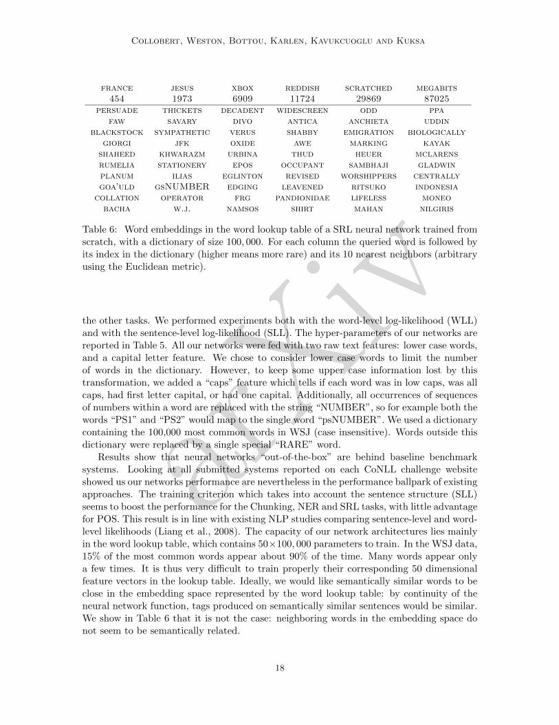
Table 6: Word embeddings in the word lookup table of a SRL neural network trained fromscratch, with a dictionary of size 100, 000. For each column the queried word is followed byits index in the dictionary (higher means more rare) and its 10 nearest neighbors (arbitraryusing the Euclidean metric).

the other tasks. We performed experiments both with the word-level log-likelihood (WLL)and with the sentence-level log-likelihood (SLL). The hyper-parameters of our networks arereported in Table 5. All our networks were fed with two raw text features: lower case words,and a capital letter feature. We chose to consider lower case words to limit the numberof words in the dictionary. However, to keep some upper case information lost by thistransformation, we added a “caps” feature which tells if each word was in low caps, was allcaps, had first letter capital, or had one capital. Additionally, all occurrences of sequencesof numbers within a word are replaced with the string “NUMBER”, so for example both thewords “PS1” and “PS2” would map to the single word “psNUMBER”. We used a dictionarycontaining the 100,000 most common words in WSJ (case insensitive). Words outside thisdictionary were replaced by a single special “RARE” word.

Results show that neural networks “out-of-the-box” are behind baseline benchmarksystems. Looking at all submitted systems reported on each CoNLL challenge websiteshowed us our networks performance are nevertheless in the performance ballpark of existingapproaches. The training criterion which takes into account the sentence structure (SLL)seems to boost the performance for the Chunking, NER and SRL tasks, with little advantagefor POS. This result is in line with existing NLP studies comparing sentence-level and word-level likelihoods (Liang et al., 2008). The capacity of our network architectures lies mainlyin the word lookup table, which contains 50×100, 000 parameters to train. In the WSJ data,15% of the most common words appear about 90% of the time. Many words appear onlya few times. It is thus very difficult to train properly their corresponding 50 dimensionalfeature vectors in the lookup table. Ideally, we would like semantically similar words to beclose in the embedding space represented by the word lookup table: by continuity of theneural network function, tags produced on semantically similar sentences would be similar.We show in Table 6 that it is not the case: neighboring words in the embedding space donot seem to be semantically related.

18

arXiv


95.5

96

96.5

100 300 500 700 900

(a) POS

90

90.5

91

91.5

100 300 500 700 900

(b) CHUNK

85

85.5

86

86.5

100 300 500 700 900

(c) NER

67

67.5

68

68.5

69

100 300 500 700 900

(d) SRL

Figure 4: F1 score on the validation set (y-axis) versus number of hidden units (x-axis)for different tasks trained with the sentence-level likelihood (SLL), as in Table 4. For SRL,we vary in this graph only the number of hidden units in the second layer. The scale isadapted for each task. We show the standard deviation (obtained over 5 runs with differentrandom initialization), for the architecture we picked (300 hidden units for POS, CHUNKand NER, 500 for SRL).

We will focus in the next section on improving these word embeddings by leveragingunlabeled data. We will see our approach results in a performance boost for all tasks.

Remark 8 (Architectures) In all our experiments in this paper, we tuned the hyper-parameters by trying only a few different architectures by validation. In practice, the choiceof hyperparameters such as the number of hidden units, provided they are large enough, hasa limited impact on the generalization performance. In Figure 4, we report the F1 scorefor each task on the validation set, with respect to the number of hidden units. Consideringthe variance related to the network initialization, we chose the smallest network achieving“reasonable” performance, rather than picking the network achieving the top performanceobtained on a single run.

Remark 9 (Training Time) Training our network is quite computationally expensive.Chunking and NER take about one hour to train, POS takes few hours, and SRL takesabout three days. Training could be faster with a larger learning rate, but we prefered tostick to a small one which works, rather than finding the optimal one for speed. Secondorder methods (LeCun et al., 1998) could be another speedup technique.

4. Lots of Unlabeled Data

We would like to obtain word embeddings carrying more syntactic and semantic informationthan shown in Table 6. Since most of the trainable parameters of our system are associatedwith the word embeddings, these poor results suggest that we should use considerablymore training data. Following our NLP from scratch philosophy, we now describe howto dramatically improve these embeddings using large unlabeled datasets. We then usethese improved embeddings to initialize the word lookup tables of the networks describedin Section 3.4.

19

arXiv


4.1 Datasets

Our first English corpus is the entire English Wikipedia.11 We have removed all paragraphscontaining non-roman characters and all MediaWiki markups. The resulting text wastokenized using the Penn Treebank tokenizer script.12 The resulting dataset contains about631 million words. As in our previous experiments, we use a dictionary containing the100,000 most common words in WSJ, with the same processing of capitals and numbers.Again, words outside the dictionary were replaced by the special “RARE” word.

Our second English corpus is composed by adding an extra 221 million words extractedfrom the Reuters RCV1 (Lewis et al., 2004) dataset.13 We also extended the dictionary to130, 000 words by adding the 30, 000 most common words in Reuters. This is useful in orderto determine whether improvements can be achieved by further increasing the unlabeleddataset size.

4.2 Ranking Criterion versus Entropy Criterion

We used these unlabeled datasets to train language models that compute scores describingthe acceptability of a piece of text. These language models are again large neural networksusing the window approach described in Section 3.2.1 and in Figure 1. As in the previoussection, most of the trainable parameters are located in the lookup tables.

Similar language models were already proposed by Bengio and Ducharme (2001) andSchwenk and Gauvain (2002). Their goal was to estimate the probability of a word giventhe previous words in a sentence. Estimating conditional probabilities suggests a cross-entropy criterion similar to those described in Section 3.3.1. Because the dictionary size islarge, computing the normalization term can be extremely demanding, and sophisticatedapproximations are required. More importantly for us, neither work leads to significantword embeddings being reported.

Shannon (1951) has estimated the entropy of the English language between 0.6 and 1.3bits per character by asking human subjects to guess upcoming characters. Cover and King(1978) give a lower bound of 1.25 bits per character using a subtle gambling approach.Meanwhile, using a simple word trigram model, Brown et al. (1992b) reach 1.75 bits percharacter. Teahan and Cleary (1996) obtain entropies as low as 1.46 bits per characterusing variable length character n-grams. The human subjects rely of course on all theirknowledge of the language and of the world. Can we learn the grammatical structure of theEnglish language and the nature of the world by leveraging the 0.2 bits per character thatseparate human subjects from simple n-gram models? Since such tasks certainly requirehigh capacity models, obtaining sufficiently small confidence intervals on the test set entropymay require prohibitively large training sets.14 The entropy criterion lacks dynamical rangebecause its numerical value is largely determined by the most frequent phrases. In order tolearn syntax, rare but legal phrases are no less significant than common phrases.

11. Available at http://download.wikimedia.org. We took the November 2007 version.12. Available at http://www.cis.upenn.edu/~treebank/tokenization.html.13. Now available at http://trec.nist.gov/data/reuters/reuters.html.14. However, Klein and Manning (2002) describe a rare example of realistic unsupervised grammar induction

using a cross-entropy approach on binary-branching parsing trees, that is, by forcing the system togenerate a hierarchical representation.

20

http://download.wikimedia.org

http://www.cis.upenn.edu/~treebank/tokenization.html

http://trec.nist.gov/data/reuters/reuters.html

arXiv


It is therefore desirable to define alternative training criteria. We propose here to use apairwise ranking approach (Cohen et al., 1998). We seek a network that computes a higherscore when given a legal phrase than when given an incorrect phrase. Because the rankingliterature often deals with information retrieval applications, many authors define complexranking criteria that give more weight to the ordering of the best ranking instances (seeBurges et al., 2007; Clemencon and Vayatis, 2007). However, in our case, we do not wantto emphasize the most common phrase over the rare but legal phrases. Therefore we use asimple pairwise criterion.

We consider a window approach network, as described in Section 3.2.1 and Figure 1,with parameters θ which outputs a score fθ(x) given a window of text x = [w]dwin1 . Weminimize the ranking criterion with respect to θ:

θ 7→∑x∈X

∑w∈D

max{

0 , 1− fθ(x) + fθ(x(w))

}, (18)

where X is the set of all possible text windows with dwin words coming from our trainingcorpus, D is the dictionary of words, and x(w) denotes the text window obtained by replacingthe central word of text window [w]dwin1 by the word w.

Okanohara and Tsujii (2007) use a related approach to avoiding the entropy criteriausing a binary classification approach (correct/incorrect phrase). Their work focuses onusing a kernel classifier, and not on learning word embeddings as we do here. Smith andEisner (2005) also propose a contrastive criterion which estimates the likelihood of the dataconditioned to a “negative” neighborhood. They consider various data neighborhoods,including sentences of length dwin drawn from Ddwin . Their goal was however to performwell on some tagging task on fully unsupervised data, rather than obtaining generic wordembeddings useful for other tasks.

4.3 Training Language Models

The language model network was trained by stochastic gradient minimization of the rankingcriterion (18), sampling a sentence-word pair (s, w) at each iteration.

Since training times for such large scale systems are counted in weeks, it is not feasibleto try many combinations of hyperparameters. It also makes sense to speed up the trainingtime by initializing new networks with the embeddings computed by earlier networks. Inparticular, we found it expedient to train a succession of networks using increasingly largedictionaries, each network being initialized with the embeddings of the previous network.Successive dictionary sizes and switching times are chosen arbitrarily. (Bengio et al., 2009)provides a more detailed discussion of this, the (as yet, poorly understood) “curriculum”process.

For the purposes of model selection we use the process of “breeding”. The idea ofbreeding is instead of trying a full grid search of possible values (which we did not haveenough computing power for) to search for the parameters in anology to breeding biologicalcell lines. Within each line, child networks are initialized with the embeddings of theirparents and trained on increasingly rich datasets with sometimes different parameters. Thatis, suppose we have k processors, which is much less than the possible set of parametersone would like to try. One chooses k initial parameter choices from the large set, and trains

21

arXiv


these on the k processors. In our case, possible parameters to adjust are: the learning rateλ, the word embedding dimensions d, number of hidden units n1

hu and input window sizedwin. One then trains each of these models in an online fashion for a certain amount oftime (i.e. a few days), and then selects the best ones using the validation set error rate.That is, breeding decisions were made on the basis of the value of the ranking criterion (18)estimated on a validation set composed of one million words held out from the Wikipediacorpus. In the next breeding iteration, one then chooses another set of k parameters fromthe possible grid of values that permute slightly the most successful candidates from theprevious round. As many of these parameter choices can share weights, we can effectivelycontinue online training retaining some of the learning from the previous iterations.

Very long training times make such strategies necessary for the foreseeable future: if wehad been given computers ten times faster, we probably would have found uses for datasetsten times bigger. However, we should say we believe that although we ended up with aparticular choice of parameters, many other choices are almost equally as good, althoughperhaps there are others that are better as we could not do a full grid search.

In the following subsections, we report results obtained with two trained languagemodels. The results achieved by these two models are representative of those achievedby networks trained on the full corpuses.

• Language model LM1 has a window size dwin = 11 and a hidden layer with n1hu = 100

units. The embedding layers were dimensioned like those of the supervised networks(Table 5). Model LM1 was trained on our first English corpus (Wikipedia) usingsuccessive dictionaries composed of the 5000, 10, 000, 30, 000, 50, 000 and finally100, 000 most common WSJ words. The total training time was about four weeks.

• Language model LM2 has the same dimensions. It was initialized with the embeddingsof LM1, and trained for an additional three weeks on our second English corpus(Wikipedia+Reuters) using a dictionary size of 130,000 words.

4.4 Embeddings

Both networks produce much more appealing word embeddings than in Section 3.4. Table 7shows the ten nearest neighbors of a few randomly chosen query words for the LM1 model.The syntactic and semantic properties of the neighbors are clearly related to those of thequery word. These results are far more satisfactory than those reported in Table 7 forembeddings obtained using purely supervised training of the benchmark NLP tasks.

4.5 Semi-supervised Benchmark Results

Semi-supervised learning has been the object of much attention during the last few years (seeChapelle et al., 2006). Previous semi-supervised approaches for NLP can be roughlycategorized as follows:

• Ad-hoc approaches such as (Rosenfeld and Feldman, 2007) for relation extraction.

• Self-training approaches, such as (Ueffing et al., 2007) for machine translation,and (McClosky et al., 2006) for parsing. These methods augment the labeled training

22

arXiv


france jesus xbox reddish scratched megabits454 1973 6909 11724 29869 87025

austria god amiga greenish nailed octetsbelgium sati playstation bluish smashed mb/sgermany christ msx pinkish punched bit/sitaly satan ipod purplish popped baud

greece kali sega brownish crimped caratssweden indra psNUMBER greyish scraped kbit/snorway vishnu hd grayish screwed megahertzeurope ananda dreamcast whitish sectioned megapixelshungary parvati geforce silvery slashed gbit/s

switzerland grace capcom yellowish ripped amperes

Table 7: Word embeddings in the word lookup table of the language model neural networkLM1 trained with a dictionary of size 100, 000. For each column the queried word is followedby its index in the dictionary (higher means more rare) and its 10 nearest neighbors (usingthe Euclidean metric, which was chosen arbitrarily).

set with examples from the unlabeled dataset using the labels predicted by the modelitself. Transductive approaches, such as (Joachims, 1999) for text classification canbe viewed as a refined form of self-training.

• Parameter sharing approaches such as (Ando and Zhang, 2005; Suzuki and Isozaki,2008). Ando and Zhang propose a multi-task approach where they jointly trainmodels sharing certain parameters. They train POS and NER models together with alanguage model (trained on 15 million words) consisting of predicting words given thesurrounding tokens. Suzuki and Isozaki embed a generative model (Hidden MarkovModel) inside a CRF for POS, Chunking and NER. The generative model is trainedon one billion words. These approaches should be seen as a linear counterpart of ourwork. Using multilayer models vastly expands the parameter sharing opportunities(see Section 5).

Our approach simply consists of initializing the word lookup tables of the supervisednetworks with the embeddings computed by the language models. Supervised training isthen performed as in Section 3.4. In particular the supervised training stage is free tomodify the lookup tables. This sequential approach is computationally convenient becauseit separates the lengthy training of the language models from the relatively fast training ofthe supervised networks. Once the language models are trained, we can perform multipleexperiments on the supervised networks in a relatively short time. Note that our procedureis clearly linked to the (semi-supervised) deep learning procedures of (Hinton et al., 2006;Bengio et al., 2007; Weston et al., 2008).

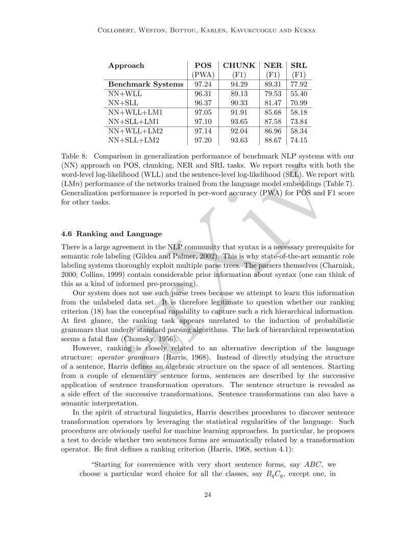
Table 8 clearly shows that this simple initialization significantly boosts the generalizationperformance of the supervised networks for each task. It is worth mentioning the largerlanguage model led to even better performance. This suggests that we could still takeadvantage of even bigger unlabeled datasets.

23

arXiv


Approach POS CHUNK NER SRL(PWA) (F1) (F1) (F1)


NN+WLL 96.31 89.13 79.53 55.40NN+SLL 96.37 90.33 81.47 70.99

NN+WLL+LM1 97.05 91.91 85.68 58.18NN+SLL+LM1 97.10 93.65 87.58 73.84

NN+WLL+LM2 97.14 92.04 86.96 58.34NN+SLL+LM2 97.20 93.63 88.67 74.15

Table 8: Comparison in generalization performance of benchmark NLP systems with our(NN) approach on POS, chunking, NER and SRL tasks. We report results with both theword-level log-likelihood (WLL) and the sentence-level log-likelihood (SLL). We report with(LMn) performance of the networks trained from the language model embeddings (Table 7).Generalization performance is reported in per-word accuracy (PWA) for POS and F1 scorefor other tasks.

4.6 Ranking and Language

There is a large agreement in the NLP community that syntax is a necessary prerequisite forsemantic role labeling (Gildea and Palmer, 2002). This is why state-of-the-art semantic rolelabeling systems thoroughly exploit multiple parse trees. The parsers themselves (Charniak,2000; Collins, 1999) contain considerable prior information about syntax (one can think ofthis as a kind of informed pre-processing).

Our system does not use such parse trees because we attempt to learn this informationfrom the unlabeled data set. It is therefore legitimate to question whether our rankingcriterion (18) has the conceptual capability to capture such a rich hierarchical information.At first glance, the ranking task appears unrelated to the induction of probabilisticgrammars that underly standard parsing algorithms. The lack of hierarchical representationseems a fatal flaw (Chomsky, 1956).

However, ranking is closely related to an alternative description of the languagestructure: operator grammars (Harris, 1968). Instead of directly studying the structureof a sentence, Harris defines an algebraic structure on the space of all sentences. Startingfrom a couple of elementary sentence forms, sentences are described by the successiveapplication of sentence transformation operators. The sentence structure is revealed asa side effect of the successive transformations. Sentence transformations can also have asemantic interpretation.

In the spirit of structural linguistics, Harris describes procedures to discover sentencetransformation operators by leveraging the statistical regularities of the language. Suchprocedures are obviously useful for machine learning approaches. In particular, he proposesa test to decide whether two sentences forms are semantically related by a transformationoperator. He first defines a ranking criterion (Harris, 1968, section 4.1):

“Starting for convenience with very short sentence forms, say ABC, wechoose a particular word choice for all the classes, say BqCq, except one, in

24

arXiv


this case A; for every pair of members Ai, Aj of that word class we ask howthe sentence formed with one of the members, i.e. AiBqCq compares as toacceptability with the sentence formed with the other member, i.e. AjBqCq.”

These gradings are then used to compare sentence forms:

“It now turns out that, given the graded n-tuples of words for a particularsentence form, we can find other sentences forms of the same word classes inwhich the same n-tuples of words produce the same grading of sentences.”

This is an indication that these two sentence forms exploit common words with the samesyntactic function and possibly the same meaning. This observation forms the empiricalbasis for the construction of operator grammars that describe real-world natural languagessuch as English.

Therefore there are solid reasons to believe that the ranking criterion (18) has theconceptual potential to capture strong syntactic and semantic information. On the otherhand, the structure of our language models is probably too restrictive for such goals, andour current approach only exploits the word embeddings discovered during training.

5. Multi-Task Learning

It is generally accepted that features trained for one task can be useful for related tasks. Thisidea was already exploited in the previous section when certain language model features,namely the word embeddings, were used to initialize the supervised networks.

Multi-task learning (MTL) leverages this idea in a more systematic way. Models forall tasks of interests are jointly trained with an additional linkage between their trainableparameters in the hope of improving the generalization error. This linkage can take the formof a regularization term in the joint cost function that biases the models towards commonrepresentations. A much simpler approach consists in having the models share certainparameters defined a priori. Multi-task learning has a long history in machine learning andneural networks. Caruana (1997) gives a good overview of these past efforts.

5.1 Joint Decoding versus Joint Training

Multitask approaches do not necessarily involve joint training. For instance, modern speechrecognition systems use Bayes rule to combine the outputs of an acoustic model trained onspeech data and a language model trained on phonetic or textual corpora (Jelinek, 1976).This joint decoding approach has been successfully applied to structurally more complexNLP tasks. Sutton and McCallum (2005b) obtains improved results by combining thepredictions of independently trained CRF models using a joint decoding process at testtime that requires more sophisticated probabilistic inference techniques. On the otherhand, Sutton and McCallum (2005a) obtain results somewhat below the state-of-the-artusing joint decoding for SRL and syntactic parsing. Musillo and Merlo (2006) also describea negative result at the same joint task.

Joint decoding invariably works by considering additional probabilistic dependencypaths between the models. Therefore it defines an implicit supermodel that describesall the tasks in the same probabilistic framework. Separately training a submodel only

25

arXiv



Benchmark Systems 97.24 94.29 89.31 –

Window ApproachNN+SLL+LM2 97.20 93.63 88.67 –NN+SLL+LM2+MTL 97.22 94.10 88.62 –

Sentence ApproachNN+SLL+LM2 97.12 93.37 88.78 74.15NN+SLL+LM2+MTL 97.22 93.75 88.27 74.29

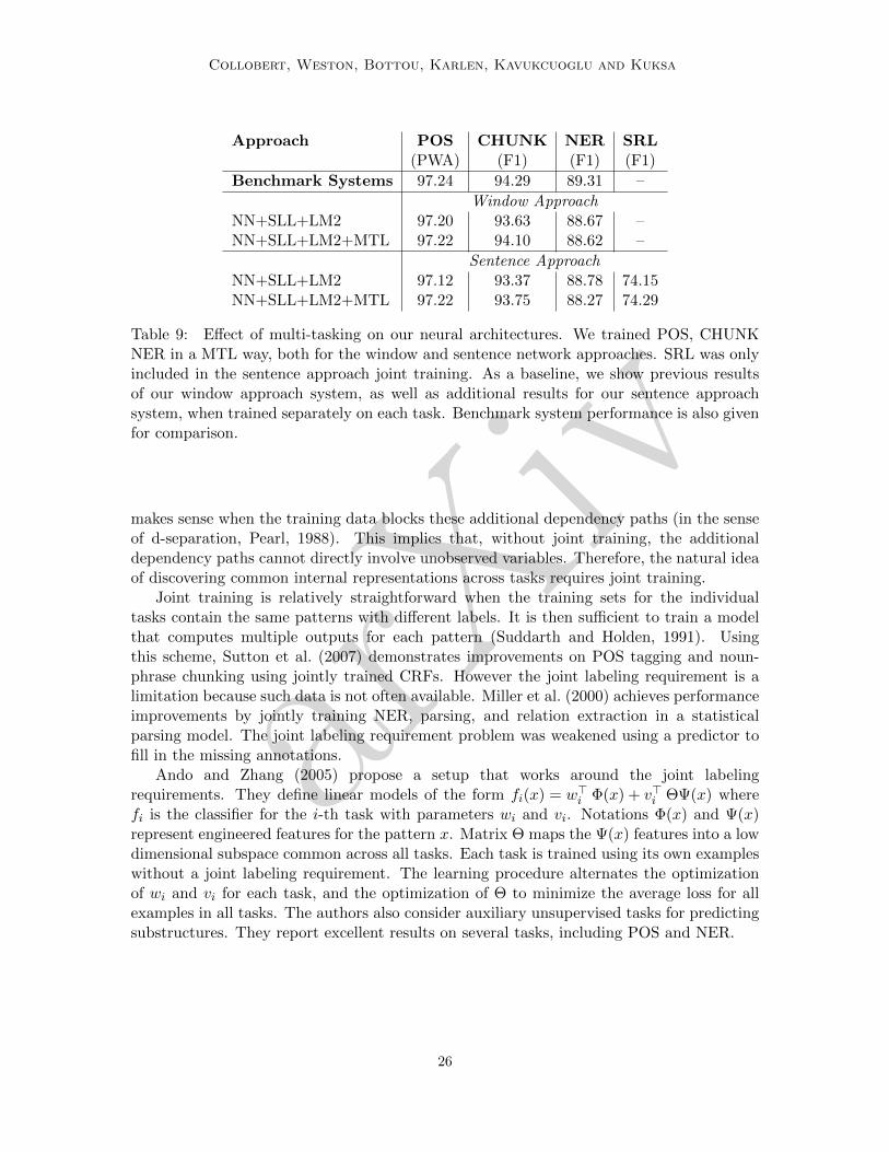
Table 9: Effect of multi-tasking on our neural architectures. We trained POS, CHUNKNER in a MTL way, both for the window and sentence network approaches. SRL was onlyincluded in the sentence approach joint training. As a baseline, we show previous resultsof our window approach system, as well as additional results for our sentence approachsystem, when trained separately on each task. Benchmark system performance is also givenfor comparison.

makes sense when the training data blocks these additional dependency paths (in the senseof d-separation, Pearl, 1988). This implies that, without joint training, the additionaldependency paths cannot directly involve unobserved variables. Therefore, the natural ideaof discovering common internal representations across tasks requires joint training.

Joint training is relatively straightforward when the training sets for the individualtasks contain the same patterns with different labels. It is then sufficient to train a modelthat computes multiple outputs for each pattern (Suddarth and Holden, 1991). Usingthis scheme, Sutton et al. (2007) demonstrates improvements on POS tagging and noun-phrase chunking using jointly trained CRFs. However the joint labeling requirement is alimitation because such data is not often available. Miller et al. (2000) achieves performanceimprovements by jointly training NER, parsing, and relation extraction in a statisticalparsing model. The joint labeling requirement problem was weakened using a predictor tofill in the missing annotations.

Ando and Zhang (2005) propose a setup that works around the joint labelingrequirements. They define linear models of the form fi(x) = w>i Φ(x) + v>i ΘΨ(x) wherefi is the classifier for the i-th task with parameters wi and vi. Notations Φ(x) and Ψ(x)represent engineered features for the pattern x. Matrix Θ maps the Ψ(x) features into a lowdimensional subspace common across all tasks. Each task is trained using its own exampleswithout a joint labeling requirement. The learning procedure alternates the optimizationof wi and vi for each task, and the optimization of Θ to minimize the average loss for allexamples in all tasks. The authors also consider auxiliary unsupervised tasks for predictingsubstructures. They report excellent results on several tasks, including POS and NER.

26

arXiv


Lookup Table

Linear

Lookup Table

Linear

HardTanh HardTanh

Linear

Task 1

Linear

Task 2

M2(t1) × · M2

(t2) × ·

LTW 1

...

LTWK

M1 × ·n1hu n1

hu

n2hu,(t1)

= #tags n2hu,(t2)

= #tags

Figure 5: Example of multitasking with NN. Task 1 and Task 2 are two tasks trained withthe window approach architecture presented in Figure 1. Lookup tables as well as the firsthidden layer are shared. The last layer is task specific. The principle is the same with morethan two tasks.

5.2 Multi-Task Benchmark Results

Table 9 reports results obtained by jointly trained models for the POS, CHUNK, NER andSRL tasks using the same setup as Section 4.5. We trained jointly POS, CHUNK and NERusing the window approach network. As we mentioned earlier, SRL can be trained onlywith the sentence approach network, due to long-range dependencies related to the verbpredicate. We thus also trained all four tasks using the sentence approach network. Inboth cases, all models share the lookup table parameters (2). The parameters of the firstlinear layers (4) were shared in the window approach case (see Figure 5), and the first theconvolution layer parameters (6) were shared in the sentence approach networks.

For the window approach, best results were obtained by enlarging the first hidden layersize to n1

hu = 500 (chosen by validation) in order to account for its shared responsibilities.We used the same architecture than SRL for the sentence approach network. The wordembedding dimension was kept constant d0 = 50 in order to reuse the language modelsof Section 4.5.

Training was achieved by minimizing the loss averaged across all tasks. This is easilyachieved with stochastic gradient by alternatively picking examples for each task andapplying (17) to all the parameters of the corresponding model, including the sharedparameters. Note that this gives each task equal weight. Since each task uses the trainingsets described in Table 1, it is worth noticing that examples can come from quite different

27

arXiv


Approach POS CHUNK NER SRL(PWA) (F1) (F1)


NN+SLL+LM2 97.20 93.63 88.67 74.15

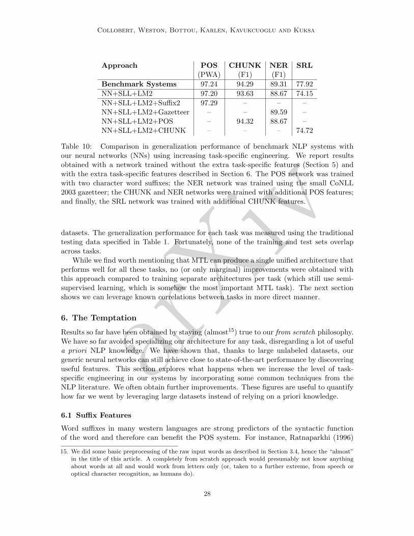
NN+SLL+LM2+Suffix2 97.29 – – –NN+SLL+LM2+Gazetteer – – 89.59 –NN+SLL+LM2+POS – 94.32 88.67 –NN+SLL+LM2+CHUNK – – – 74.72

Table 10: Comparison in generalization performance of benchmark NLP systems withour neural networks (NNs) using increasing task-specific engineering. We report resultsobtained with a network trained without the extra task-specific features (Section 5) andwith the extra task-specific features described in Section 6. The POS network was trainedwith two character word suffixes; the NER network was trained using the small CoNLL2003 gazetteer; the CHUNK and NER networks were trained with additional POS features;and finally, the SRL network was trained with additional CHUNK features.

datasets. The generalization performance for each task was measured using the traditionaltesting data specified in Table 1. Fortunately, none of the training and test sets overlapacross tasks.

While we find worth mentioning that MTL can produce a single unified architecture thatperforms well for all these tasks, no (or only marginal) improvements were obtained withthis approach compared to training separate architectures per task (which still use semi-supervised learning, which is somehow the most important MTL task). The next sectionshows we can leverage known correlations between tasks in more direct manner.

6. The Temptation

Results so far have been obtained by staying (almost15) true to our from scratch philosophy.We have so far avoided specializing our architecture for any task, disregarding a lot of usefula priori NLP knowledge. We have shown that, thanks to large unlabeled datasets, ourgeneric neural networks can still achieve close to state-of-the-art performance by discoveringuseful features. This section explores what happens when we increase the level of task-specific engineering in our systems by incorporating some common techniques from theNLP literature. We often obtain further improvements. These figures are useful to quantifyhow far we went by leveraging large datasets instead of relying on a priori knowledge.

6.1 Suffix Features

Word suffixes in many western languages are strong predictors of the syntactic functionof the word and therefore can benefit the POS system. For instance, Ratnaparkhi (1996)

15. We did some basic preprocessing of the raw input words as described in Section 3.4, hence the “almost”in the title of this article. A completely from scratch approach would presumably not know anythingabout words at all and would work from letters only (or, taken to a further extreme, from speech oroptical character recognition, as humans do).

28

arXiv


uses inputs representing word suffixes and prefixes up to four characters. We achieve thisin the POS task by adding discrete word features (Section 3.1.1) representing the last twocharacters of every word. The size of the suffix dictionary was 455. This led to a smallimprovement of the POS performance (Table 10, row NN+SLL+LM2+Suffix2). We also triedsuffixes obtained with the Porter (1980) stemmer and obtained the same performance aswhen using two character suffixes.

6.2 Gazetteers

State-of-the-art NER systems often use a large dictionary containing well known namedentities (e.g. Florian et al., 2003). We restricted ourselves to the gazetteer providedby the CoNLL challenge, containing 8, 000 locations, person names, organizations, andmiscellaneous entities. We trained a NER network with 4 additional word features indicating(feature “on” or “off”) whether the word is found in the gazetteer under one of these fourcategories. The gazetteer includes not only words, but also chunks of words. If a sentencechunk is found in the gazetteer, then all words in the chunk have their correspondinggazetteer feature turned to “on”. The resulting system displays a clear performanceimprovement (Table 10, row NN+SLL+LM2+Gazetteer), slightly outperforming the baseline.A plausible explanation of this large boost over the network using only the language modelis that gazeetters include word chunks, while we use only the word representation of ourlanguage model. For example, “united” and “bicycle” seen separately are likely to be non-entities, while “united bicycle” might be an entity, but catching it would require higherlevel representations of our language model.

6.3 Cascading

When one considers related tasks, it is reasonable to assume that tags obtained for one taskcan be useful for taking decisions in the other tasks. Conventional NLP systems often usefeatures obtained from the output of other preexisting NLP systems. For instance, Shenand Sarkar (2005) describe a chunking system that uses POS tags as input; Florian et al.(2003) describes a NER system whose inputs include POS and CHUNK tags, as well asthe output of two other NER classifiers. State-of-the-art SRL systems exploit parse trees(Gildea and Palmer, 2002; Punyakanok et al., 2005), related to CHUNK tags, and builtusing POS tags (Charniak, 2000; Collins, 1999).

Table 10 reports results obtained for the CHUNK and NER tasks by adding discreteword features (Section 3.1.1) representing the POS tags. In order to facilitate comparisons,instead of using the more accurate tags from our POS network, we use for each task thePOS tags provided by the corresponding CoNLL challenge. We also report results obtainedfor the SRL task by adding word features representing the CHUNK tags (also provided bythe CoNLL challenge). We consistently obtain moderate improvements.

6.4 Ensembles

Constructing ensembles of classifiers is a proven way to trade computational efficiency forgeneralization performance (Bell et al., 2007). Therefore it is not surprising that manyNLP systems achieve state-of-the-art performance by combining the outputs of multiple

29

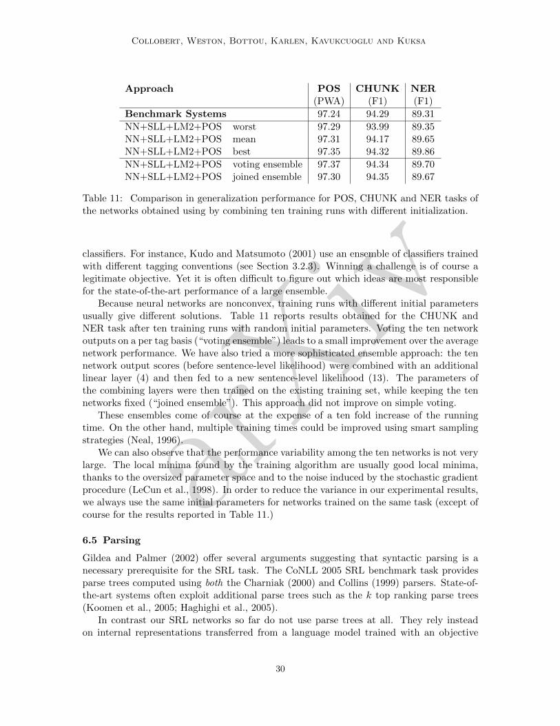
arXiv


Approach POS CHUNK NER(PWA) (F1) (F1)

Benchmark Systems 97.24 94.29 89.31

NN+SLL+LM2+POS worst 97.29 93.99 89.35NN+SLL+LM2+POS mean 97.31 94.17 89.65NN+SLL+LM2+POS best 97.35 94.32 89.86

NN+SLL+LM2+POS voting ensemble 97.37 94.34 89.70NN+SLL+LM2+POS joined ensemble 97.30 94.35 89.67

Table 11: Comparison in generalization performance for POS, CHUNK and NER tasks ofthe networks obtained using by combining ten training runs with different initialization.

classifiers. For instance, Kudo and Matsumoto (2001) use an ensemble of classifiers trainedwith different tagging conventions (see Section 3.2.3). Winning a challenge is of course alegitimate objective. Yet it is often difficult to figure out which ideas are most responsiblefor the state-of-the-art performance of a large ensemble.

Because neural networks are nonconvex, training runs with different initial parametersusually give different solutions. Table 11 reports results obtained for the CHUNK andNER task after ten training runs with random initial parameters. Voting the ten networkoutputs on a per tag basis (“voting ensemble”) leads to a small improvement over the averagenetwork performance. We have also tried a more sophisticated ensemble approach: the tennetwork output scores (before sentence-level likelihood) were combined with an additionallinear layer (4) and then fed to a new sentence-level likelihood (13). The parameters ofthe combining layers were then trained on the existing training set, while keeping the tennetworks fixed (“joined ensemble”). This approach did not improve on simple voting.

These ensembles come of course at the expense of a ten fold increase of the runningtime. On the other hand, multiple training times could be improved using smart samplingstrategies (Neal, 1996).

We can also observe that the performance variability among the ten networks is not verylarge. The local minima found by the training algorithm are usually good local minima,thanks to the oversized parameter space and to the noise induced by the stochastic gradientprocedure (LeCun et al., 1998). In order to reduce the variance in our experimental results,we always use the same initial parameters for networks trained on the same task (except ofcourse for the results reported in Table 11.)

6.5 Parsing

Gildea and Palmer (2002) offer several arguments suggesting that syntactic parsing is anecessary prerequisite for the SRL task. The CoNLL 2005 SRL benchmark task providesparse trees computed using both the Charniak (2000) and Collins (1999) parsers. State-of-the-art systems often exploit additional parse trees such as the k top ranking parse trees(Koomen et al., 2005; Haghighi et al., 2005).

In contrast our SRL networks so far do not use parse trees at all. They rely insteadon internal representations transferred from a language model trained with an objective

30

arXiv


level 0

S

NP

The luxury auto makerb-np i-np i-np e-np

NP

last yearb-np e-np

VP

solds-vp

NP

1,214 carsb-np e-np

PP

ins-pp

NP

the U.S.b-np e-np

level 1

S

The luxury auto maker last yearo o o o o o

VP

sold 1,214 carsb-vp i-vp e-vp

PP

in the U.S.b-pp i-pp e-pp

level 2

S

The luxury auto maker last yearo o o o o o

VP

sold 1,214 cars in the U.S.b-vp i-vp i-vp i-vp i-vp e-vp

Figure 6: Charniak parse tree for the sentence “The luxury auto maker last year sold 1,214cars in the U.S.”. Level 0 is the original tree. Levels 1 to 4 are obtained by successivelycollapsing terminal tree branches. For each level, words receive tags describing the segmentassociated with the corresponding leaf. All words receive tag “O” at level 3 in this example.

function that captures a lot of syntactic information (see Section 4.6). It is thereforelegitimate to question whether this approach is an acceptable lightweight replacement forparse trees.

We answer this question by providing parse tree information as additional input featuresto our system. We have limited ourselves to the Charniak parse tree provided with theCoNLL 2005 data. Considering that a node in a syntactic parse tree assigns a labelto a segment of the parsed sentence, we propose a way to feed (partially) this labeledsegmentation to our network, through additional lookup tables. Each of these lookuptables encode labeled segments of each parse tree level (up to a certain depth). The labeledsegments are fed to the network following a IOBES tagging scheme (see Sections 3.2.3and 3.1.1). As there are 40 different phrase labels in WSJ, each additional tree-relatedlookup tables has 161 entries (40× 4 + 1) corresponding to the IBES segment tags, plus theextra O tag.

We call level 0 the information associated with the leaves of the original Charniak parsetree. The lookup table for level 0 encodes the corresponding IOBES phrase tags for eachwords. We obtain levels 1 to 4 by repeatedly trimming the leaves as shown in Figure 6. Welabeled “O” words belonging to the root node “S”, or all words of the sentence if the rootitself has been trimmed.

Experiments were performed using the LM2 language model using the same networkarchitectures (see Table 5) and using additional lookup tables of dimension 5 for each

31

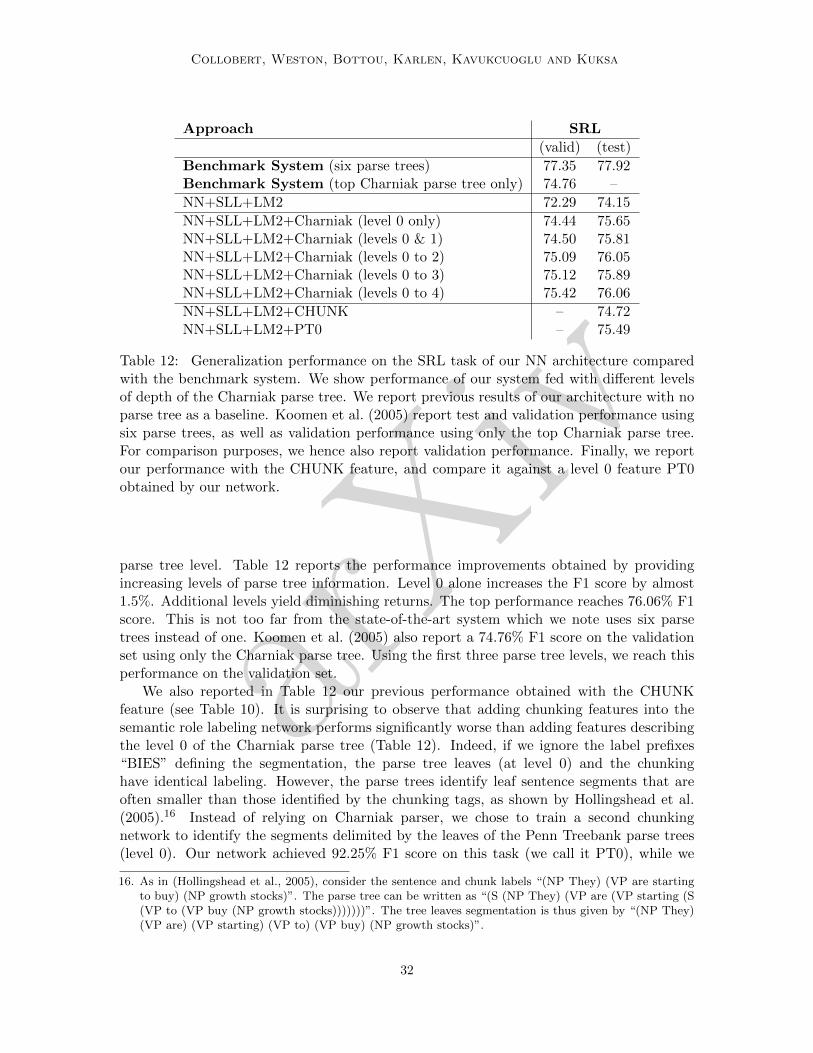
arXiv


Approach SRL

(valid) (test)

Benchmark System (six parse trees) 77.35 77.92Benchmark System (top Charniak parse tree only) 74.76 –

NN+SLL+LM2 72.29 74.15

NN+SLL+LM2+Charniak (level 0 only) 74.44 75.65NN+SLL+LM2+Charniak (levels 0 & 1) 74.50 75.81NN+SLL+LM2+Charniak (levels 0 to 2) 75.09 76.05NN+SLL+LM2+Charniak (levels 0 to 3) 75.12 75.89NN+SLL+LM2+Charniak (levels 0 to 4) 75.42 76.06

NN+SLL+LM2+CHUNK – 74.72NN+SLL+LM2+PT0 – 75.49

Table 12: Generalization performance on the SRL task of our NN architecture comparedwith the benchmark system. We show performance of our system fed with different levelsof depth of the Charniak parse tree. We report previous results of our architecture with noparse tree as a baseline. Koomen et al. (2005) report test and validation performance usingsix parse trees, as well as validation performance using only the top Charniak parse tree.For comparison purposes, we hence also report validation performance. Finally, we reportour performance with the CHUNK feature, and compare it against a level 0 feature PT0obtained by our network.

parse tree level. Table 12 reports the performance improvements obtained by providingincreasing levels of parse tree information. Level 0 alone increases the F1 score by almost1.5%. Additional levels yield diminishing returns. The top performance reaches 76.06% F1score. This is not too far from the state-of-the-art system which we note uses six parsetrees instead of one. Koomen et al. (2005) also report a 74.76% F1 score on the validationset using only the Charniak parse tree. Using the first three parse tree levels, we reach thisperformance on the validation set.

We also reported in Table 12 our previous performance obtained with the CHUNKfeature (see Table 10). It is surprising to observe that adding chunking features into thesemantic role labeling network performs significantly worse than adding features describingthe level 0 of the Charniak parse tree (Table 12). Indeed, if we ignore the label prefixes“BIES” defining the segmentation, the parse tree leaves (at level 0) and the chunkinghave identical labeling. However, the parse trees identify leaf sentence segments that areoften smaller than those identified by the chunking tags, as shown by Hollingshead et al.(2005).16 Instead of relying on Charniak parser, we chose to train a second chunkingnetwork to identify the segments delimited by the leaves of the Penn Treebank parse trees(level 0). Our network achieved 92.25% F1 score on this task (we call it PT0), while we

16. As in (Hollingshead et al., 2005), consider the sentence and chunk labels “(NP They) (VP are startingto buy) (NP growth stocks)”. The parse tree can be written as “(S (NP They) (VP are (VP starting (S(VP to (VP buy (NP growth stocks)))))))”. The tree leaves segmentation is thus given by “(NP They)(VP are) (VP starting) (VP to) (VP buy) (NP growth stocks)”.

32

arXiv


evaluated Charniak performance as 91.94% on the same task. As shown in Table 12, feedingour own PT0 prediction into the SRL system gives similar performance to using Charniakpredictions, and is consistently better than the CHUNK feature.

6.6 Word Representations

In Section 4, we adapted our neural network architecture for training a language model task.By leveraging a large amount of unlabeled text data, we induced word embeddings whichwere shown to boost generalization performance on all tasks. While we chose to stick withone single architecture, other ways to induce word representations exist. Mnih and Hinton(2007) proposed a related language model approach inspired from Restricted BoltzmannMachines. However, word representations are perhaps more commonly infered from n-gramlanguage modelling rather than smoothed language models. One popular approach is theBrown clustering algorithm (Brown et al., 1992a), which builds hierachical word clustersby maximizing the bigram’s mutual information. The induced word representation hasbeen used with success in a wide variety of NLP tasks, including POS (Schutze, 1995),NER (Miller et al., 2004; Ratinov and Roth, 2009), or parsing (Koo et al., 2008). Otherrelated approaches exist, like phrase clustering (Lin and Wu, 2009) which has been shownto work well for NER. Finally, Huang and Yates (2009) have recently proposed a smoothedlanguage modelling approach based on a Hidden Markov Model, with success on POS andChunking tasks.

While a comparison of all these word representations is beyond the scope of this paper,it is rather fair to question the quality of our word embeddings compared to a popular NLPapproach. In this section, we report a comparison of our word embeddings against Brownclusters, when used as features into our neural network architecture. We report as baselineprevious results where our word embeddings are fine-tuned for each task. We also reportperformance when our embeddings are kept fixed during task-specific training. Since convexmachine learning algorithms are common practice in NLP, we finally report performancesfor the convex version of our architecture.

For the convex experiments, we considered the linear version of our neural networks(instead of having several linear layers interleaved with a non-linearity). While we alwayspicked the sentence approach for SRL, we had to consider the window approach in thisparticular convex setup, as the sentence approach network (see Figure 2) includes a Maxlayer. Having only one linear layer in our neural network is not enough to make ourarchitecture convex: all lookup-tables (for each discrete feature) must also be fixed. Theword-lookup table is simply fixed to the embeddings obtained from our language modelLM2. All other discrete feature lookup-tables (caps, POS, Brown Clusters...) are fixed to astandard sparse representation. Using the notation introduced in Section 3.1.1, if LTWk is

the lookup-table of the kth discrete feature, we have W k ∈ R|Dk|×|Dk| and the representationof the discrete input w is obtained with:

LTWk(w) = 〈W k〉1w =

(0, · · · 0, 1

at index w, 0, · · · 0

)T

. (19)

Training our architecture in this convex setup with the sentence-level likelihood (13)corresponds to training a CRF. In that respect, these convex experiments show theperformance of our word embeddings in a classical NLP framework.

33

arXiv



Non-convex ApproachLM2 (non-linear NN) 97.29 94.32 89.59 76.06LM2 (non-linear NN, fixed embeddings) 97.10 94.45 88.79 72.24Brown Clusters (non-linear NN, 130K words) 96.92 94.35 87.15 72.09Brown Clusters (non-linear NN, all words) 96.81 94.21 86.68 71.44

Convex ApproachLM2 (linear NN, fixed embeddings) 96.69 93.51 86.64 59.11Brown Clusters (linear NN, 130K words) 96.56 94.20 86.46 51.54Brown Clusters (linear NN, all words) 96.28 94.22 86.63 56.42

Table 13: Generalization performance of our neural network architecture trained withour language model (LM2) word embeddings, and with the word representations derivedfrom the Brown Clusters. As before, all networks are fed with a capitalization feature.Additionally, POS is using a word suffix of size 2 feature, CHUNK is fed with POS, NERuses the CoNLL 2003 gazetteer, and SRL is fed with levels 1–5 of the Charniak parse tree,as well as a verb position feature. We report performance with both convex and non-convexarchitectures (300 hidden units for all tasks, with an additional 500 hidden units layer forSRL). We also provide results for Brown Clusters induced with a 130K word dictionary, aswell as Brown Clusters induced with all words of the given tasks.

Following the Ratinov and Roth (2009) and Koo et al. (2008) setups, we generated 1, 000Brown clusters using the implementation17 from Liang (2005). To make the comparisonfair, the clusters were first induced on the concatenation of Wikipedia and Reuters datasets,as we did in Section 4 for training our largest language model LM2, using a 130K worddictionary. This dictionary covers about 99% of the words in the training set of each task.To cover the last 1%, we augmented the dictionary with the missing words (reaching about140K words) and induced Brown Clusters using the concatenation of WSJ, Wikipedia, andReuters.

The Brown clustering approach is hierarchical and generates a binary tree of clusters.Each word in the vocabulary is assigned to a node in the tree. Features are extracted fromthis tree by considering the path from the root to the node containing the word of interest.Following Ratinov & Roth, we picked as features the path prefixes of size 4, 6, 10 and 20. Inthe non-convex experiments, we fed these four Brown Cluster features to our architectureusing four different lookup tables, replacing our word lookup table. The size of the lookuptables was chosen to be 12 by validation. In the convex case, we used the classical sparserepresentation (19), as for any other discrete feature.

We first report in Table 13 generalization performance of our best non-convex networkstrained with our LM2 language model and with Brown Cluster features. Our embeddingsperform at least as well as Brown Clusters. Results are more mitigated in a convex setup.For most task, going non-convex is better for both word representation types. In general,

17. Available at http://www.eecs.berkeley.edu/~pliang/software.

34

http://www.eecs.berkeley.edu/~pliang/software

arXiv


Task Features

POS Suffix of size 2CHUNK POSNER CoNLL 2003 gazetteerPT0 POSSRL PT0, verb position

Table 14: Features used by SENNA implementation, for each task. In addition, all tasksuse “low caps word” and “caps” features.

“fine-tuning” our embeddings for each task also gives an extra boost. Finally, using a betterword coverage with Brown Clusters (“all words” instead of “130K words” in Table 13) didnot help.

More complex features could be possibly combined instead of using a non-linearmodel. For instance, Turian et al. (2010) performed a comparison of Brown Clusters andembeddings trained in the same spirit as ours18, with additional features combining labelsand tokens. We believe this type of comparison should be taken with care, as combininga given feature with different word representations might not have the same effect on eachword representation.

6.7 Engineering a Sweet Spot

We implemented a standalone version of our architecture, written in the C language.We gave the name “SENNA” (Semantic/syntactic Extraction using a Neural NetworkArchitecture) to the resulting system. The parameters of each architecture are the onesdescribed in Table 5. All the networks were trained separately on each task using thesentence-level likelihood (SLL). The word embeddings were initialized to LM2 embeddings,and then fine-tuned for each task. We summarize features used by our implementationin Table 14, and we report performance achieved on each task in Table 15. The runtimeversion19 contains about 2500 lines of C code, runs in less than 150MB of memory, and needsless than a millisecond per word to compute all the tags. Table 16 compares the taggingspeeds for our system and for the few available state-of-the-art systems: the Toutanova et al.(2003) POS tagger20, the Shen et al. (2007) POS tagger21 and the Koomen et al. (2005) SRLsystem.22 All programs were run on a single 3GHz Intel core. The POS taggers were runwith Sun Java 1.6 with a large enough memory allocation to reach their top tagging speed.

18. However they did not reach our embedding performance. There are several differences in how theytrained their models that might explain this. Firstly, they may have experienced difficulties becausethey train 50-dimensional embeddings for 269K distinct words using a comparatively small training set(RCV1, 37M words), unlikely to contain enough instances of the rare words. Secondly, they predict thecorrectness of the final word of each window instead of the center word (Turian et al., 2010), effectivelyrestricting the model to unidirectional prediction. Finally, they do not fine tune their embeddings afterunsupervised training.

19. Available at http://ml.nec-labs.com/senna.20. Available at http://nlp.stanford.edu/software/tagger.shtml. We picked the 3.0 version (May 2010).21. Available at http://www.cis.upenn.edu/~xtag/spinal.22. Available at http://l2r.cs.uiuc.edu/~cogcomp/asoftware.php?skey=SRL.

35

http://ml.nec-labs.com/senna

http://nlp.stanford.edu/software/tagger.shtml

http://www.cis.upenn.edu/~xtag/spinal

http://l2r.cs.uiuc.edu/~cogcomp/asoftware.php?skey=SRL

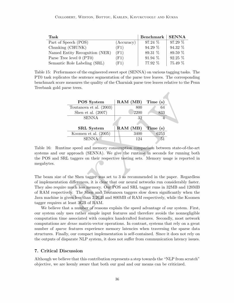
arXiv


Task Benchmark SENNA

Part of Speech (POS) (Accuracy) 97.24 % 97.29 %Chunking (CHUNK) (F1) 94.29 % 94.32 %Named Entity Recognition (NER) (F1) 89.31 % 89.59 %Parse Tree level 0 (PT0) (F1) 91.94 % 92.25 %Semantic Role Labeling (SRL) (F1) 77.92 % 75.49 %

Table 15: Performance of the engineered sweet spot (SENNA) on various tagging tasks. ThePT0 task replicates the sentence segmentation of the parse tree leaves. The correspondingbenchmark score measures the quality of the Charniak parse tree leaves relative to the PennTreebank gold parse trees.

POS System RAM (MB) Time (s)

Toutanova et al. (2003) 800 64Shen et al. (2007) 2200 833

SENNA 32 4

SRL System RAM (MB) Time (s)

Koomen et al. (2005) 3400 6253

SENNA 124 51

Table 16: Runtime speed and memory consumption comparison between state-of-the-artsystems and our approach (SENNA). We give the runtime in seconds for running boththe POS and SRL taggers on their respective testing sets. Memory usage is reported inmegabytes.

The beam size of the Shen tagger was set to 3 as recommended in the paper. Regardlessof implementation differences, it is clear that our neural networks run considerably faster.They also require much less memory. Our POS and SRL tagger runs in 32MB and 120MBof RAM respectively. The Shen and Toutanova taggers slow down significantly when theJava machine is given less than 2.2GB and 800MB of RAM respectively, while the Koomentagger requires at least 3GB of RAM.

We believe that a number of reasons explain the speed advantage of our system. First,our system only uses rather simple input features and therefore avoids the nonnegligiblecomputation time associated with complex handcrafted features. Secondly, most networkcomputations are dense matrix-vector operations. In contrast, systems that rely on a greatnumber of sparse features experience memory latencies when traversing the sparse datastructures. Finally, our compact implementation is self-contained. Since it does not rely onthe outputs of disparate NLP system, it does not suffer from communication latency issues.

7. Critical Discussion

Although we believe that this contribution represents a step towards the “NLP from scratch”objective, we are keenly aware that both our goal and our means can be criticized.

36

arXiv


The main criticism of our goal can be summarized as follows. Over the years, the NLPcommunity has developed a considerable expertise in engineering effective NLP features.Why should they forget this painfully acquired expertise and instead painfully acquirethe skills required to train large neural networks? As mentioned in our introduction, weobserve that no single NLP task really covers the goals of NLP. Therefore we believe thattask-specific engineering (i.e. that does not generalize to other tasks) is not desirable. Butwe also recognize how much our neural networks owe to previous NLP task-specific research.

The main criticism of our means is easier to address. Why did we choose to rely on atwenty year old technology, namely multilayer neural networks? We were simply attractedby their ability to discover hidden representations using a stochastic learning algorithmthat scales linearly with the number of examples. Most of the neural network technologynecessary for our work has been described ten years ago (e.g. Le Cun et al., 1998). However,if we had decided ten years ago to train the language model network LM2 using a vintagecomputer, training would only be nearing completion today. Training algorithms that scalelinearly are most able to benefit from such tremendous progress in computer hardware.

8. Conclusion

We have presented a multilayer neural network architecture that can handle a number ofNLP tasks with both speed and accuracy. The design of this system was determined byour desire to avoid task-specific engineering as much as possible. Instead we rely on largeunlabeled datasets and let the training algorithm discover internal representations thatprove useful for all the tasks of interest. Using this strong basis, we have engineered a fastand efficient “all purpose” NLP tagger that we hope will prove useful to the community.

Acknowledgments

We acknowledge the persistent support of NEC for this research effort. We thank YoshuaBengio, Samy Bengio, Eric Cosatto, Vincent Etter, Hans-Peter Graf, Ralph Grishman, andVladimir Vapnik for their useful feedback and comments.

37

arXiv


Appendix A. Neural Network Gradients

We consider a neural network fθ(·), with parameters θ. We maximize the likelihood (8), orminimize ranking criterion (18), with respect to the parameters θ, using stochastic gradient.By negating the likelihood, we now assume it all corresponds to minimize a cost C(fθ(·)),with respect to θ.

Following the classical “back-propagation” derivations (LeCun, 1985; Rumelhart et al.,1986) and the modular approach shown in (Bottou, 1991), any feed-forward neural networkwith L layers, like the ones shown in Figure 1 and Figure 2, can be seen as a compositionof functions f lθ(·), corresponding to each layer l:

fθ(·) = fLθ (fL−1θ (. . . f1

θ (·) . . .))

Partionning the parameters of the network with respect to each layers 1 ≤ l ≤ L, we write:

θ = (θ1, . . . , θl, . . . , θL) .

We are now interested in computing the gradients of the cost with respect to each θl.Applying the chain rule (generalized to vectors) we obtain the classical backpropagationrecursion:

∂C

∂θl=

∂f lθ∂θl

∂C

∂f lθ(20)

∂C

∂f l−1θ

=∂f lθ∂f l−1

θ

∂C

∂f lθ. (21)

In other words, we first initialize the recursion by computing the gradient of the cost withrespect to the last layer output ∂C/∂fLθ . Then each layer l computes the gradient respectto its own parameters with (20), given the gradient coming from its output ∂C/∂f lθ. Toperform the backpropagation, it also computes the gradient with respect to its own inputs,as shown in (21). We now derive the gradients for each layer we used in this paper.

Lookup Table Layer Given a matrix of parameters θ1 = W 1 and word (or discretefeature) indices [w]T1 , the layer outputs the matrix:

f lθ([w]Tl ) =(〈W 〉1[w]1

〈W 〉1[w]2. . . 〈W 〉1[w]T

).

The gradients of the weights 〈W 〉1i are given by:

∂C

∂〈W 〉1i=

∑{1≤t≤T / [w]t=i}

〈 ∂C∂f lθ〉1i

This sum equals zero if the index i in the lookup table does not corresponds to a word inthe sequence. In this case, the ith column of W does not need to be updated. As a LookupTable Layer is always the first layer, we do not need to compute its gradients with respectto the inputs.

38

arXiv


Linear Layer Given parameters θl = (W l, bl), and an input vector f l−1θ the output is

given by:f lθ = W lf l−1

θ + bl . (22)

The gradients with respect to the parameters are then obtained with:

∂C

∂W l=

[∂C

∂f lθ

] [f l−1θ

]Tand

∂C

∂bl=∂C

∂f lθ, (23)

and the gradients with respect to the inputs are computed with:

∂C

∂f l−1θ

=[W l]T ∂C∂f lθ

. (24)

Convolution Layer Given a input matrix f l−1θ , a Convolution Layer f lθ(·) applies a

Linear Layer operation (22) successively on each window 〈f l−1θ 〉dwint (1 ≤ t ≤ T ) of size

dwin. Using (23), the gradients of the parameters are thus given by summing over allwindows:

∂C

∂W l=

T∑t=1

[〈 ∂C∂f lθ〉1t] [〈f l−1θ 〉dwint

]Tand

∂C

∂bl=

T∑t=1

〈 ∂C∂f lθ〉1t .

After initializing the input gradients ∂C/∂f l−1θ to zero, we iterate (24) over all windows for

1 ≤ t ≤ T , leading the accumulation23:

〈 ∂C∂f l−1

θ

〉dwint +=[W l]T〈 ∂C∂f lθ〉1t .

Max Layer Given a matrix f l−1θ , the Max Layer computes[

f lθ

]i

= maxt

[〈f l−1θ 〉1t

]i

and ai = argmaxt

[〈f l−1θ 〉1t

]i∀i ,

where ai stores the index of the largest value. We only need to compute the gradient withrespect to the inputs, as this layer has no parameters. The gradient is given by[

〈 ∂C∂f l−1

θ

〉1t

]i

=

{ [〈 ∂C∂f lθ〉1t]i

if t = ai

0 otherwise.

HardTanh Layer Given a vector f l−1θ , and the definition of the HardTanh (5) we get

[∂C

∂f l−1θ

]i

=

0 if

[f l−1θ

]i< −1[

∂C∂f lθ

]i

if − 1 <=[f l−1θ

]i<= 1

0 if[f l−1θ

]i> 1

,

if we ignore non-differentiability points.

23. We denote “+=” any accumulation operation.

39

arXiv


Word-Level Log-Likelihood The network outputs a score [fθ]i for each tag indexed byi. Following (11), if y is the true tag for a given example, the stochastic score to minimizecan be written as

C(fθ) = logaddj

[fθ]j − [fθ]y

Considering the definition of the logadd (10), the gradient with respect to fθ is given by

∂C

∂ [fθ]i=

e[fθ]i∑k e

[fθ]k− 1i=y ∀i.

Sentence-Level Log-Likelihood The network outputs a matrix where each element[fθ]i, t gives a score for tag i at word t. Given a tag sequence [y]T1 and a input sequence [x]T1 ,

we maximize the likelihood (13), which corresponds to minimizing the score

C(fθ, A) = logadd∀[j]T1

s([x]T1 , [j]T1 , θ)︸︷︷︸Clogadd

−s([x]T1 , [y]T1 , θ) ,

with

s([x]T1 , [y]T1 , θ) =T∑t=1

([A][y]t−1, [y]t

+ [fθ][y]t, t

).

We first initialize all gradients to zero

∂C

∂[fθ]i, t

= 0 ∀i, t and∂C

∂ [A]i, j= 0 ∀i, j .

We then accumulate gradients over the second part of the cost −s([x]T1 , [y]T1 , θ), whichgives:

∂C

∂[fθ][y]t, t

+= 1

∂C

∂ [A][y]t−1, [y]t

+= 1

∀t .

We now need to accumulate the gradients over the first part of the cost, that is Clogadd.We differentiate Clogadd by applying the chain rule through the recursion (14). First weinitialize our recursion with

∂Clogadd∂δT (i)

=eδT (i)∑k e

δT (k)∀i .

We then compute iteratively:

∂Clogadd∂δt−1(i)

=∑j

∂Clogadd∂δt(j)

eδt−1(i)+[A]i, j∑k e

δt−1(k)+[A]k, j, (25)

40

arXiv


where at each step t of the recursion we accumulate of the gradients with respect to theinputs fθ, and the transition scores [A]i, j :

∂C

∂[fθ]i, t

+=∂Clogadd∂δt(i)

∂δt(i)

∂[fθ]i, t

=∂Clogadd∂δt(i)

∂C

∂ [A]i, j+=

∂Clogadd∂δt(j)

∂δt(j)

∂ [A]i, j=∂Clogadd∂δt(j)

eδt−1(i)+[A]i, j∑k e

δt−1(k)+[A]k, j.

Ranking Criterion We use the ranking criterion (18) for training our language model.In this case, given a “positive” example x and a “negative” example x(w), we want tominimize:

C(fθ(x), fθ(xw)) = max

{0 , 1− fθ(x) + fθ(x

(w))}. (26)

Ignoring the non-differentiability of max(0, ·) in zero, the gradient is simply given by:

( ∂C∂fθ(x)

∂C∂fθ(xw)

)=

(−1

1

)if 1− fθ(x) + fθ(x

(w)) > 0(0

0

)otherwise

.

References

R. K. Ando and T. Zhang. A framework for learning predictive structures from multipletasks and unlabeled data. JMLR, 6:1817–1953, 11 2005.

R. M. Bell, Y. Koren, and C. Volinsky. The BellKor solution to the Netflix Prize. Technicalreport, AT&T Labs, 2007. http://www.research.att.com/~volinsky/netflix.

Y. Bengio and R. Ducharme. A neural probabilistic language model. In NIPS 13, 2001.

Y. Bengio, P. Lamblin, D. Popovici, and H. Larochelle. Greedy layer-wise training of deepnetworks. In Advances in Neural Information Processing Systems, NIPS 19, 2007.

Y. Bengio, J. Louradour, R. Collobert, and J. Weston. Curriculum learning. In InternationalConference on Machine Learning, ICML, 2009.

L. Bottou. Stochastic gradient learning in neural networks. In Proceedings of Neuro-Nımes91, Nimes, France, 1991. EC2.

L. Bottou. Online algorithms and stochastic approximations. In David Saad, editor, OnlineLearning and Neural Networks. Cambridge University Press, Cambridge, UK, 1998.

L. Bottou and P. Gallinari. A framework for the cooperation of learning algorithms. InD. Touretzky and R. Lippmann, editors, Advances in Neural Information ProcessingSystems, volume 3. Morgan Kaufmann, Denver, 1991.

L. Bottou, Y. LeCun, and Yoshua Bengio. Global training of document processing systemsusing graph transformer networks. In Proc. of Computer Vision and Pattern Recognition,pages 489–493, Puerto-Rico, 1997. IEEE.

41

http://www.research.att.com/~volinsky/netflix

arXiv


J. S. Bridle. Probabilistic interpretation of feedforward classification network outputs, withrelationships to statistical pattern recognition. In F. Fogelman Soulie and J. Herault,editors, Neurocomputing: Algorithms, Architectures and Applications, pages 227–236.NATO ASI Series, 1990.

P. F. Brown, P. V. deSouza, R. L. Mercer, V. J. D. Pietra, and J C. Lai. Class-based n-grammodels of natural language. Computational Linguistics, 18(4):467–479, 1992a.

P. F. Brown, V. J. Della Pietra, R. L. Mercer, S. A. Della Pietra, and J. C. Lai. An estimateof an upper bound for the entropy of english. Computational Linguistics, 18(1):31–41,1992b.

C. J. C. Burges, R. Ragno, and Quoc Viet Le. Learning to rank with nonsmooth costfunctions. In B. Scholkopf, J. Platt, and T. Hoffman, editors, Advances in NeuralInformation Processing Systems 19, pages 193–200. MIT Press, Cambridge, MA, 2007.

R. Caruana. Multitask Learning. Machine Learning, 28(1):41–75, 1997.

O. Chapelle, B. Schlkopf, and A. Zien. Semi-Supervised Learning. Adaptive computationand machine learning. MIT Press, Cambridge, Mass., USA, 09 2006.

E. Charniak. A maximum-entropy-inspired parser. Proceedings of the first conference onNorth American chapter of the Association for Computational Linguistics, pages 132–139,2000.

H. L. Chieu. Named entity recognition with a maximum entropy approach. In In Proceedingsof the Seventh Conference on Natural Language Learning (CoNLL-2003, pages 160–163,2003.

N. Chomsky. Three models for the description of language. IRE Transactions onInformation Theory, 2(3):113–124, September 1956.

S. Clemencon and N. Vayatis. Ranking the best instances. Journal of Machine LearningResearch, 8:2671–2699, December 2007.

W. W. Cohen, R. E. Schapire, and Y. Singer. Learning to order things. Journal of ArtificialIntelligence Research, 10:243–270, 1998.

T. Cohn and P. Blunsom. Semantic role labelling with tree conditional random fields. InNinth Conference on Computational Natural Language (CoNLL), 2005.

M. Collins. Head-Driven Statistical Models for Natural Language Parsing. PhD thesis,University of Pennsylvania, 1999.

R. Collobert. Large Scale Machine Learning. PhD thesis, Universite Paris VI, 2004.

T. Cover and R. King. A convergent gambling estimate of the entropy of english. IEEETransactions on Information Theory, 24(4):413–421, July 1978.

42

arXiv


R. Florian, A. Ittycheriah, H. Jing, and T. Zhang. Named entity recognition throughclassifier combination. In Proceedings of the seventh conference on Natural languagelearning at HLT-NAACL 2003, pages 168–171. Association for Computational Linguistics,2003.

D. Gildea and D. Jurafsky. Automatic labeling of semantic roles. Computational Linguistics,28(3):245–288, 2002.

D. Gildea and M. Palmer. The necessity of parsing for predicate argument recognition.Proceedings of the 40th Annual Meeting of the ACL, pages 239–246, 2002.

J. Gimenez and L. Marquez. SVMTool: A general POS tagger generator based onsupport vector machines. In Proceedings of the 4th International Conference on LanguageResources and Evaluation (LREC’04), 2004.

A. Haghighi, K. Toutanova, and C. D. Manning. A joint model for semantic role labeling.In Proceedings of the Ninth Conference on Computational Natural Language Learning(CoNLL-2005). Association for Computational Linguistics, June 2005.

Z. S. Harris. Mathematical Structures of Language. John Wiley & Sons Inc., 1968.

D. Heckerman, D. M. Chickering, C. Meek, R. Rounthwaite, and C. Kadie. Dependencynetworks for inference, collaborative filtering, and data visualization. Journal of MachineLearning Research, 1:49–75, 2001. ISSN 1532-4435.

G. E. Hinton, S. Osindero, and Y.-W. Teh. A fast learning algorithm for deep belief nets.Neural Comp., 18(7):1527–1554, July 2006.

K. Hollingshead, S. Fisher, and B. Roark. Comparing and combining finite-state andcontext-free parsers. In HLT ’05: Proceedings of the conference on Human LanguageTechnology and Empirical Methods in Natural Language Processing, pages 787–794.Association for Computational Linguistics, 2005.

F. Huang and A. Yates. Distributional representations for handling sparsity in supervisedsequence-labeling. In Proceedings of the Association for Computational Linguistics(ACL), pages 495–503. Association for Computational Linguistics, 2009.

F. Jelinek. Continuous speech recognition by statistical methods. Proceedings of the IEEE,64(4):532–556, 1976.

T. Joachims. Transductive inference for text classification using support vector machines.In ICML, 1999.

D. Klein and C. D. Manning. Natural language grammar induction using a constituent-context model. In Thomas G. Dietterich, Suzanna Becker, and Zoubin Ghahramani,editors, Advances in Neural Information Processing Systems 14, pages 35–42. MIT Press,Cambridge, MA, 2002.

T. Koo, X. Carreras, and M. Collins. Simple semi-supervised dependency parsing. InProceedings of the Association for Computational Linguistics (ACL), pages 595–603, 2008.

43

arXiv


P. Koomen, V. Punyakanok, D. Roth, and W. Yih. Generalized inference with multiplesemantic role labeling systems (shared task paper). In Ido Dagan and Dan Gildea, editors,Proc. of the Annual Conference on Computational Natural Language Learning (CoNLL),pages 181–184, 2005.

T. Kudo and Y. Matsumoto. Chunking with support vector machines. In In Proceedingsof the 2nd Meeting of the North American Association for Computational Linguistics:NAACL 2001, pages 1–8. Association for Computational Linguistics, 2001.

T. Kudoh and Y. Matsumoto. Use of support vector learning for chunk identification. InProceedings of CoNLL-2000 and LLL-2000, pages 142–144, 2000.

J. Lafferty, A. McCallum, and F. Pereira. Conditional random fields: Probabilistic modelsfor segmenting and labeling sequence data. In Eighteenth International Conference onMachine Learning, ICML, 2001.

Y. Le Cun, L. Bottou, Y. Bengio, and P. Haffner. Gradient based learning applied todocument recognition. Proceedings of IEEE, 86(11):2278–2324, 1998.

Y. LeCun. A learning scheme for asymmetric threshold networks. In Proceedings ofCognitiva 85, pages 599–604, Paris, France, 1985.

Y. LeCun, L. Bottou, G. B. Orr, and K.-R. Muller. Efficient backprop. In G.B. Orr andK.-R. Muller, editors, Neural Networks: Tricks of the Trade, pages 9–50. Springer, 1998.

D. D. Lewis, Y. Yang, T. G. Rose, and F. Li. Rcv1: A new benchmark collection for textcategorization research. Journal of Machine Learning Research, 5:361–397, 2004.

P. Liang. Semi-supervised learning for natural language. Master’s thesis, MassachusettsInstitute of Technology, 2005.

P. Liang, H. Daume, III, and D. Klein. Structure compilation: trading structure for features.In International conference on Machine learning (ICML), pages 592–599. ACM, 2008.

D. Lin and X. Wu. Phrase clustering for discriminative learning. In Proceedings ofthe Association for Computational Linguistics (ACL), pages 1030–1038. Association forComputational Linguistics, 2009.

N. Littlestone. Learning quickly when irrelevant attributes abound: A new linear-thresholdalgorithm. In Machine Learning, pages 285–318, 1988.

A. McCallum and Wei Li. Early results for named entity recognition with conditionalrandom fields, feature induction and web-enhanced lexicons. In Proceedings of theseventh conference on Natural language learning at HLT-NAACL 2003, pages 188–191.Association for Computational Linguistics, 2003.

D. McClosky, E. Charniak, and M. Johnson. Effective self-training for parsing. Proceedingsof HLT-NAACL 2006, 2006.

44

arXiv


R. McDonald, K. Crammer, and F. Pereira. Flexible text segmentation with structuredmultilabel classification. In HLT ’05: Proceedings of the conference on Human LanguageTechnology and Empirical Methods in Natural Language Processing, pages 987–994.Association for Computational Linguistics, 2005.

S. Miller, H. Fox, L. Ramshaw, and R. Weischedel. A novel use of statistical parsing toextract information from text. 6th Applied Natural Language Processing Conference,2000.

S. Miller, J. Guinness, and A. Zamanian. Name tagging with word clusters anddiscriminative training. In Proceedings of HLT-NAACL, pages 337–342, 2004.

A Mnih and G. E. Hinton. Three new graphical models for statistical language modelling.In International Conference on Machine Learning, ICML, pages 641–648, 2007.

G. Musillo and P. Merlo. Robust Parsing of the Proposition Bank. ROMAND 2006: RobustMethods in Analysis of Natural language Data, 2006.

R. M. Neal. Bayesian Learning for Neural Networks. Number 118 in Lecture Notes inStatistics. Springer-Verlag, New York, 1996.

D. Okanohara and J. Tsujii. A discriminative language model with pseudo-negative samples.Proceedings of the 45th Annual Meeting of the ACL, pages 73–80, 2007.

M. Palmer, D. Gildea, and P. Kingsbury. The proposition bank: An annotated corpus ofsemantic roles. Comput. Linguist., 31(1):71–106, 2005. ISSN 0891-2017.

J. Pearl. Probabilistic Reasoning in Intelligent Systems. Morgan Kaufman, San Mateo,1988.

D. C. Plaut and G. E. Hinton. Learning sets of filters using back-propagation. ComputerSpeech and Language, 2:35–61, 1987.

M. F. Porter. An algorithm for suffix stripping. Program, 14(3):130–137, 1980.

S. Pradhan, W. Ward, K. Hacioglu, J. Martin, and D. Jurafsky. Shallow semantic parsingusing support vector machines. Proceedings of HLT/NAACL-2004, 2004.

S. Pradhan, K. Hacioglu, W. Ward, J. H. Martin, and D. Jurafsky. Semantic role chunkingcombining complementary syntactic views. In Proceedings of the Ninth Conference onComputational Natural Language Learning (CoNLL-2005), pages 217–220. Associationfor Computational Linguistics, June 2005.

V. Punyakanok, D. Roth, and W. Yih. The necessity of syntactic parsing for semantic rolelabeling. In IJCAI, pages 1117–1123, 2005.

L. Ratinov and D. Roth. Design challenges and misconceptions in named entity recognition.In Proceedings of the Thirteenth Conference on Computational Natural Language Learning(CoNLL), pages 147–155. Association for Computational Linguistics, 2009.

45

arXiv


A. Ratnaparkhi. A maximum entropy model for part-of-speech tagging. In Eric Brill andKenneth Church, editors, Proceedings of the Conference on Empirical Methods in NaturalLanguage Processing, pages 133–142. Association for Computational Linguistics, 1996.

B. Rosenfeld and R. Feldman. Using Corpus Statistics on Entities to Improve Semi-supervised Relation Extraction from the Web. Proceedings of the 45th Annual Meetingof the ACL, pages 600–607, 2007.

D. E. Rumelhart, G. E. Hinton, and R. J. Williams. Learning internal representationsby back-propagating errors. In D.E. Rumelhart and J. L. McClelland, editors, ParallelDistributed Processing: Explorations in the Microstructure of Cognition, volume 1, pages318–362. MIT Press, 1986.

H. Schutze. Distributional part-of-speech tagging. In Proceedings of the Association forComputational Linguistics (ACL), pages 141–148. Morgan Kaufmann Publishers Inc.,1995.

H. Schwenk and J. L. Gauvain. Connectionist language modeling for large vocabularycontinuous speech recognition. In IEEE International Conference on Acoustics, Speech,and Signal Processing, pages 765–768, 2002.

F. Sha and F. Pereira. Shallow parsing with conditional random fields. In NAACL ’03:Proceedings of the 2003 Conference of the North American Chapter of the Association forComputational Linguistics on Human Language Technology, pages 134–141. Associationfor Computational Linguistics, 2003.

C. E. Shannon. Prediction and entropy of printed english. Bell Systems Technical Journal,30:50–64, 1951.

H. Shen and A. Sarkar. Voting between multiple data representations for text chunking.Advances in Artificial Intelligence, pages 389–400, 2005.

L. Shen, G. Satta, and A. K. Joshi. Guided learning for bidirectional sequence classification.In Proceedings of the 45th Annual Meeting of the Association for ComputationalLinguistics (ACL), 2007.

N. A. Smith and J. Eisner. Contrastive estimation: Training log-linear models on unlabeleddata. In Proceedings of the 43rd Annual Meeting of the Association for ComputationalLinguistics (ACL), pages 354–362. Association for Computational Linguistics, 2005.

S. C. Suddarth and A. D. C. Holden. Symbolic-neural systems and the use of hints fordeveloping complex systems. International Journal of Man-Machine Studies, 35(3):291–311, 1991.

X. Sun, L.-P. Morency, D. Okanohara, and J. Tsujii. Modeling latent-dynamic in shallowparsing: a latent conditional model with improved inference. In COLING ’08: Proceedingsof the 22nd International Conference on Computational Linguistics, pages 841–848.Association for Computational Linguistics, 2008.

46

arXiv


C. Sutton and A. McCallum. Joint parsing and semantic role labeling. In Proceedings ofCoNLL-2005, pages 225–228, 2005a.

C. Sutton and A. McCallum. Composition of conditional random fields for transfer learning.Proceedings of the conference on Human Language Technology and Empirical Methods inNatural Language Processing, pages 748–754, 2005b.

C. Sutton, A. McCallum, and K. Rohanimanesh. Dynamic Conditional Random Fields:Factorized Probabilistic Models for Labeling and Segmenting Sequence Data. JMLR, 8:693–723, 2007.

J. Suzuki and H. Isozaki. Semi-supervised sequential labeling and segmentation using giga-word scale unlabeled data. In Proceedings of ACL-08: HLT, pages 665–673, Columbus,Ohio, June 2008. Association for Computational Linguistics.

W. J. Teahan and J. G. Cleary. The entropy of english using ppm-based models. In In DataCompression Conference (DCC’96), pages 53–62. IEEE Computer Society Press, 1996.

K. Toutanova, D. Klein, C. D. Manning, and Y. Singer. Feature-rich part-of-speech taggingwith a cyclic dependency network. In HLT-NAACL, 2003.

J. Turian, L. Ratinov, and Y. Bengio. Word representations: A simple and generalmethod for semi-supervised learning. In Proceedings of the Association for ComputationalLinguistics (ACL), pages 384–392. Association for Computational Linguistics, 2010.

N. Ueffing, G. Haffari, and A. Sarkar. Transductive learning for statistical machinetranslation. Proceedings of the 45th Annual Meeting of the ACL, pages 25–32, 2007.

A. Waibel, T. Hanazawa, G. Hinton, K. Shikano, and K.J. Lang. Phoneme recognitionusing time-delay neural networks. IEEE Transactions on Acoustics, Speech, and SignalProcessing, 37(3):328–339, 1989.

J. Weston, F. Ratle, and R. Collobert. Deep learning via semi-supervised embedding. InProceedings of the 25th international conference on Machine learning, pages 1168–1175.ACM, 2008.

47

natural language processing (almost) from scratch - arxiv · pdf filenatural language...

Documents