natural language inference a dissertation - the stanford nlp
TRANSCRIPT

NATURAL LANGUAGE INFERENCE
A DISSERTATION
SUBMITTED TO THE DEPARTMENT OF COMPUTER SCIENCE
AND THE COMMITTEE ON GRADUATE STUDIES
OF STANFORD UNIVERSITY
IN PARTIAL FULFILLMENT OF THE REQUIREMENTS
FOR THE DEGREE OF
DOCTOR OF PHILOSOPHY
Bill MacCartneyJune 2009

c© Copyright by Bill MacCartney 2009
All Rights Reserved
ii

I certify that I have read this dissertation and that, in my opinion, itis fully adequate in scope and quality as a dissertation for the degreeof Doctor of Philosophy.
(Christopher D. Manning) Principal Adviser
I certify that I have read this dissertation and that, in my opinion, itis fully adequate in scope and quality as a dissertation for the degreeof Doctor of Philosophy.
(Dan Jurafsky)
I certify that I have read this dissertation and that, in my opinion, itis fully adequate in scope and quality as a dissertation for the degreeof Doctor of Philosophy.
(Stanley Peters)
Approved for the University Committee on Graduate Studies.
iii

Abstract
Inference has been a central topic in artificial intelligence from the start, but whileautomatic methods for formal deduction have advanced tremendously, comparativelylittle progress has been made on the problem of natural language inference (NLI),that is, determining whether a natural language hypothesis h can justifiably be in-ferred from a natural language premise p. The challenges of NLI are quite differentfrom those encountered in formal deduction: the emphasis is on informal reasoning,lexical semantic knowledge, and variability of linguistic expression. This dissertationexplores a range of approaches to NLI, beginning with methods which are robust butapproximate, and proceeding to progressively more precise approaches.
We first develop a baseline system based on overlap between bags of words. Despiteits extreme simplicity, this model achieves surprisingly good results on a standard NLIevaluation, the PASCAL RTE Challenge. However, its effectiveness is limited by itsfailure to represent semantic structure.
To remedy this lack, we next introduce the Stanford RTE system, which uses typeddependency trees as a proxy for semantic structure, and seeks a low-cost alignmentbetween trees for p and h, using a cost model which incorporates both lexical andstructural matching costs. This system is typical of a category of approaches to NLIbased on approximate graph matching. We argue, however, that such methods workbest when the entailment decision is based, not merely on the degree of alignment,but also on global features of the aligned 〈p, h〉 pair motivated by semantic theory.
Seeking still greater precision, we devote the largest part of the dissertation todeveloping an approach to NLI based on natural logic. We present a new model of
iv

natural logic which extends the monotonicity calculus of van Benthem and Sánchez-Valencia to incorporate semantic exclusion and implicativity. We define an expressiveset of entailment relations—including representations of both semantic containmentand semantic exclusion—and described the algebra of their joins. We then describea model of compositional entailment capable of determining the entailment relationbetween two sentences connected by a sequence of edits. We introduce the conceptof projectivity signatures, which generalizes the concept of monotonicity classes tocover the exclusion relations. And, we show how our framework can be used to explaininferences involving implicatives and non-factives.
Next, we describe the NatLog system, a computational implementation of ourmodel of natural logic. NatLog is the first robust, general-purpose system for naturallogic inference over real English sentences. The NatLog system decomposes an infer-ence problem into a sequence of atomic edits which transforms p into h; predicts alexical entailment relation for each edit using a statistical classifier; propagates theserelations upward through a syntax tree according to semantic properties of interme-diate nodes; and joins the resulting entailment relations across the edit sequence. Wedemonstrate the practical value of the NatLog system in evaluations on the FraCaSand RTE test suites.
Finally, we address the problem of alignment for NLI, by developing a model ofphrase-based alignment inspired by analogous work in machine translation, includingan alignment scoring function, inference algorithms for finding good alignments, andtraining algorithms for choosing feature weights.
v

Acknowledgments
To write a dissertation is a mighty undertaking, and I could not have reached thefinish line without the influence, advice, and support of many colleagues, friends, andfamily. My thanks are due first and foremost to my advisor, Chris Manning, for beingwilling to take me on as a student, and for being unfailingly generous with his timeand his support throughout my graduate career. Chris provided consistently goodadvice, helped me to situate my work in a broader context, and gave me tremendousfreedom in pursuing my ideas, while always ensuring that I was making progresstoward some fruitful outcome. I will be forever grateful for his help.
I am deeply obliged to the other members of my dissertation committee for theiradvice and encouragement. From Dan Jurafsky, I received a steady stream of positivefeedback that helped to keep my motivation strong. Stanley Peters was of great helpin working out various theoretical issues, and in making connections to the literatureof formal semantics. I am indebted to Johan van Benthem not only for his pioneeringwork on the role of monotonicity in natural language inference—which was the directinspiration for my model of natural logic—but also for pushing me to consider thetheoretical implications of my work. Perceptive questions from Mike Genesereth alsohelped greatly to sharpen my ideas.
I owe special thanks to David Beaver, who first brought my attention to the topicof natural logic and the concept of monotonicity, and thereby set me on a path whichculminated in this dissertation.
The faculty, students, and visitors involved with the Stanford NLP Group haveprovided a congenial and stimulating environment in which to pursue my studies.I am particularly indebted to my frequent collaborators—including Marie-Catherine
vi

de Marneffe, Michel Galley, Teg Grenager, and many others—who shared my strug-gles and helped to shape my thoughts. I am also grateful to past officemates IddoLev, Roger Levy, Kristina Toutanova, Jeff Michels, and Dan Ramage for their warmcompanionship and for countless fascinating conversations.
Finally, I offer my deepest thanks to my siblings—Leslie, Jim, and Doug—whoselove and support has sustained me; to my parents, Louis and Sharon, who instilledin me the love of learning that has fueled all my efforts; and to Destiny, who believedin me most when I believed in myself least.
vii
Contents
Abstract iv
Acknowledgments vi
1 The problem of natural language inference 1
1.1 What is natural language inference? . . . . . . . . . . . . . . . . . . . 11.2 Applications of NLI . . . . . . . . . . . . . . . . . . . . . . . . . . . . 31.3 NLI task formulations and problem sets . . . . . . . . . . . . . . . . . 5
1.3.1 The FraCaS test suite . . . . . . . . . . . . . . . . . . . . . . 61.3.2 Recognizing Textual Entailment (RTE) . . . . . . . . . . . . . 8
1.4 Previous approaches to NLI . . . . . . . . . . . . . . . . . . . . . . . 101.4.1 Shallow approaches . . . . . . . . . . . . . . . . . . . . . . . . 101.4.2 Deep approaches . . . . . . . . . . . . . . . . . . . . . . . . . 11
1.5 The natural logic approach to NLI . . . . . . . . . . . . . . . . . . . 131.6 Overview of the dissertation . . . . . . . . . . . . . . . . . . . . . . . 14
2 The bag-of-words approach 16
2.1 A simple bag-of-words entailment model . . . . . . . . . . . . . . . . 172.1.1 Approach . . . . . . . . . . . . . . . . . . . . . . . . . . . . . 172.1.2 The lexical scoring function . . . . . . . . . . . . . . . . . . . 182.1.3 Per-word alignment costs . . . . . . . . . . . . . . . . . . . . . 202.1.4 Total alignment costs . . . . . . . . . . . . . . . . . . . . . . . 212.1.5 Predicting entailment . . . . . . . . . . . . . . . . . . . . . . . 22
2.2 Experimental results . . . . . . . . . . . . . . . . . . . . . . . . . . . 24
viii

3 Alignment for natural language inference 28
3.1 NLI alignment vs. MT alignment . . . . . . . . . . . . . . . . . . . . 293.2 The MSR alignment data . . . . . . . . . . . . . . . . . . . . . . . . . 303.3 The MANLI aligner . . . . . . . . . . . . . . . . . . . . . . . . . . . . 32
3.3.1 A phrase-based alignment representation . . . . . . . . . . . . 323.3.2 A feature-based scoring function . . . . . . . . . . . . . . . . . 343.3.3 Decoding using simulated annealing . . . . . . . . . . . . . . . 353.3.4 Perceptron learning . . . . . . . . . . . . . . . . . . . . . . . . 37
3.4 Evaluating aligners on MSR data . . . . . . . . . . . . . . . . . . . . 383.4.1 A robust baseline: the bag-of-words aligner . . . . . . . . . . . 393.4.2 MT aligners: GIZA++ and Cross-EM . . . . . . . . . . . . . 393.4.3 The Stanford RTE aligner . . . . . . . . . . . . . . . . . . . . 413.4.4 The MANLI aligner . . . . . . . . . . . . . . . . . . . . . . . . 42
3.5 Using alignment to predict RTE answers . . . . . . . . . . . . . . . . 443.6 Conclusion . . . . . . . . . . . . . . . . . . . . . . . . . . . . . . . . . 45
4 The Stanford RTE system 46
4.1 Approaching a robust semantics . . . . . . . . . . . . . . . . . . . . . 474.2 System . . . . . . . . . . . . . . . . . . . . . . . . . . . . . . . . . . . 51
4.2.1 Linguistic analysis . . . . . . . . . . . . . . . . . . . . . . . . 514.2.2 Alignment . . . . . . . . . . . . . . . . . . . . . . . . . . . . . 534.2.3 Entailment determination . . . . . . . . . . . . . . . . . . . . 54
4.3 Feature representation . . . . . . . . . . . . . . . . . . . . . . . . . . 554.4 Evaluation . . . . . . . . . . . . . . . . . . . . . . . . . . . . . . . . . 584.5 Conclusion . . . . . . . . . . . . . . . . . . . . . . . . . . . . . . . . . 60
5 Entailment relations 63
5.1 Introduction . . . . . . . . . . . . . . . . . . . . . . . . . . . . . . . . 635.2 Representations of entailment . . . . . . . . . . . . . . . . . . . . . . 64
5.2.1 Entailment as two-way classification . . . . . . . . . . . . . . . 645.2.2 Entailment as three-way classification . . . . . . . . . . . . . . 655.2.3 Entailment as a containment relation . . . . . . . . . . . . . . 66
ix

5.2.4 The best of both worlds . . . . . . . . . . . . . . . . . . . . . 685.3 The 16 elementary set relations . . . . . . . . . . . . . . . . . . . . . 70
5.3.1 Properties of the elementary set relations . . . . . . . . . . . . 725.3.2 Cardinalities of the elementary set relations . . . . . . . . . . 75
5.4 From set relations to entailment relations . . . . . . . . . . . . . . . . 765.5 The seven basic entailment relations . . . . . . . . . . . . . . . . . . . 77
5.5.1 The assumption of non-vacuity . . . . . . . . . . . . . . . . . 785.5.2 Defining the relations in B . . . . . . . . . . . . . . . . . . . . 78
5.6 Joining entailment relations . . . . . . . . . . . . . . . . . . . . . . . 805.6.1 “Nondeterministic” joins . . . . . . . . . . . . . . . . . . . . . 815.6.2 Computing joins . . . . . . . . . . . . . . . . . . . . . . . . . 825.6.3 Unions of the basic entailment relations . . . . . . . . . . . . . 84
6 Compositional entailment 86
6.1 Lexical entailment relations . . . . . . . . . . . . . . . . . . . . . . . 886.1.1 Substitutions of open-class terms . . . . . . . . . . . . . . . . 886.1.2 Substitutions of closed-class terms . . . . . . . . . . . . . . . . 906.1.3 Generic deletions and insertions . . . . . . . . . . . . . . . . . 916.1.4 Special deletions and insertions . . . . . . . . . . . . . . . . . 92
6.2 Entailments and semantic composition . . . . . . . . . . . . . . . . . 926.2.1 Semantic composition in the monotonicity calculus . . . . . . 936.2.2 Projectivity signatures . . . . . . . . . . . . . . . . . . . . . . 936.2.3 Projectivity of logical connectives . . . . . . . . . . . . . . . . 946.2.4 Projectivity of quantifiers . . . . . . . . . . . . . . . . . . . . 986.2.5 Projectivity of verbs . . . . . . . . . . . . . . . . . . . . . . . 99
6.3 Implicatives and factives . . . . . . . . . . . . . . . . . . . . . . . . . 1006.3.1 Implication signatures . . . . . . . . . . . . . . . . . . . . . . 1006.3.2 Deletions and insertions of implicatives . . . . . . . . . . . . . 1016.3.3 Deletions and insertions of factives . . . . . . . . . . . . . . . 1026.3.4 Projectivity signatures of implicatives . . . . . . . . . . . . . . 104
6.4 Putting it all together . . . . . . . . . . . . . . . . . . . . . . . . . . 105
x

6.5 Examples . . . . . . . . . . . . . . . . . . . . . . . . . . . . . . . . . 1076.5.1 An example involving exclusion . . . . . . . . . . . . . . . . . 1076.5.2 Examples involving implicatives . . . . . . . . . . . . . . . . . 1086.5.3 Different edit orders . . . . . . . . . . . . . . . . . . . . . . . 1116.5.4 Inability to handle de Morgan’s laws for quantifiers . . . . . . 1116.5.5 A more complex example . . . . . . . . . . . . . . . . . . . . . 113
6.6 Is the inference method sound? . . . . . . . . . . . . . . . . . . . . . 117
7 The NatLog system 120
7.1 System architecture . . . . . . . . . . . . . . . . . . . . . . . . . . . . 1207.2 Linguistic analysis . . . . . . . . . . . . . . . . . . . . . . . . . . . . 1227.3 Alignment . . . . . . . . . . . . . . . . . . . . . . . . . . . . . . . . . 1227.4 Predicting lexical entailment relations . . . . . . . . . . . . . . . . . . 124
7.4.1 Feature representation . . . . . . . . . . . . . . . . . . . . . . 1257.4.2 Classifier training . . . . . . . . . . . . . . . . . . . . . . . . . 131
7.5 Entailment projection . . . . . . . . . . . . . . . . . . . . . . . . . . . 1337.5.1 Monotonicity marking . . . . . . . . . . . . . . . . . . . . . . 1347.5.2 Predicting projections . . . . . . . . . . . . . . . . . . . . . . 135
7.6 Joining entailment relations . . . . . . . . . . . . . . . . . . . . . . . 1367.7 An example of NatLog in action . . . . . . . . . . . . . . . . . . . . . 1377.8 Evaluation on the FraCaS test suite . . . . . . . . . . . . . . . . . . . 140
7.8.1 Characteristics of the FraCaS test suite . . . . . . . . . . . . . 1417.8.2 Experiments and results . . . . . . . . . . . . . . . . . . . . . 1427.8.3 Discussion . . . . . . . . . . . . . . . . . . . . . . . . . . . . . 145
7.9 Evaluation on the RTE test suite . . . . . . . . . . . . . . . . . . . . 1487.9.1 Characteristics of the RTE test suite . . . . . . . . . . . . . . 1487.9.2 Experiments and results . . . . . . . . . . . . . . . . . . . . . 1497.9.3 Discussion . . . . . . . . . . . . . . . . . . . . . . . . . . . . . 151
8 Conclusions 152
8.1 Contributions of the dissertation . . . . . . . . . . . . . . . . . . . . . 1528.2 The future of natural language inference . . . . . . . . . . . . . . . . 155
xi

List of Tables
1.1 High-level characteristics of the RTE problem sets. . . . . . . . . . . 9
2.1 Performance of the bag-of-words model . . . . . . . . . . . . . . . . . 252.2 Comparable results from the first three RTE competitions . . . . . . 25
3.1 Performance of various aligners on the MSR RTE2 alignment data . . 403.2 Performance of various systems in predicting RTE2 answers . . . . . 45
4.1 Performance of various systems on the RTE1 test suite . . . . . . . . 594.2 Learned weights for selected features . . . . . . . . . . . . . . . . . . 61
5.1 The 16 elementary set relations, in terms of set-theoretic constraints . 725.2 An example of computing the join of two relations in R . . . . . . . . 845.3 The join table for the seven basic entailment relations in B . . . . . . 85
6.1 Projectivity signatures for logical connectives . . . . . . . . . . . . . . 946.2 Projectivity signatures for various binary generalized quantifiers . . . 986.3 The nine implication signatures of Nairn et al. . . . . . . . . . . . . . 1016.4 Lexical entailment relations generated by edits involving implicatives 1026.5 Monotonicity and projectivity properties of implicatives and factives . 1046.6 Analysis of an inference involving semantic exclusion . . . . . . . . . 1086.7 Analysis of an inference involving an implicative . . . . . . . . . . . . 1096.8 Analysis of another inference involving an implicative . . . . . . . . . 1096.9 Six analyses of the same inference, using different edit orders . . . . . 1106.10 Analysis of an example of de Morgan’s laws for quantifiers, first try . 112
xii

6.11 Analysis of an example of de Morgan’s laws for quantifiers, second try 1136.12 Analysis of a more complex inference, first try . . . . . . . . . . . . . 1146.13 Analysis of a more complex inference, second try . . . . . . . . . . . . 1156.14 Analysis of a more complex inference, third try . . . . . . . . . . . . 116
7.1 Examples of training problems for the lexical entailment model . . . . 1327.2 An example of the operation of the NatLog model . . . . . . . . . . . 1387.3 Performance of various systems on the FraCaS test suite . . . . . . . 1437.4 Performance of NatLog on the FraCaS test suite, by section . . . . . 1447.5 Confusion matrix for NatLog on the FraCaS test suite . . . . . . . . . 1457.6 Performance of various systems on the RTE3 test suite . . . . . . . . 150
xiii

List of Figures
1.1 Some single-premise inference problems from the FraCaS test suite . . 71.2 Some multiple-premise inference problems from the FraCaS test suite 8
2.1 Possible features for the bag-of-words model . . . . . . . . . . . . . . 24
3.1 The MSR gold standard alignment for RTE2 problem 116 . . . . . . 313.2 The MSR gold alignment for RTE2 problem 116, as phrase edits . . . 333.3 The manli-align algorithm . . . . . . . . . . . . . . . . . . . . . . . 363.4 The manli-learn algorithm . . . . . . . . . . . . . . . . . . . . . . 37
4.1 Illustrative examples from the RTE1 development set . . . . . . . . . 484.2 A typed dependency graph for problem 971 of figure 4.1 . . . . . . . 524.3 A sample alignment for problem 971 of figure 4.1 . . . . . . . . . . . 53
5.1 A comparison of three representations of entailment relations . . . . . 685.2 The 16 elementary set relations, represented by Johnston diagrams . 71
7.1 Some monotonicity operator type definitions . . . . . . . . . . . . . . 1347.2 Syntactic parses for the sentences in the James Dean example . . . . 1387.3 Examples of errors made by NatLog on the FraCaS test suite. . . . . 1467.4 Illustrative examples from the RTE3 development set . . . . . . . . . 149
xiv
Chapter 1
The problem of natural language
inference
1.1 What is natural language inference?
Natural language inference (NLI) is the problem of determining whether a naturallanguage hypothesis h can reasonably be inferred from a natural language premise p.Of course, inference has been a central topic in artificial intelligence (AI) from thestart, and over the last five decades, researchers have made tremendous progress indeveloping automatic methods for formal deduction. But the challenges of NLI arequite different from those encountered in formal deduction: the emphasis is on in-formal reasoning, lexical semantic knowledge, and variability of linguistic expression,rather than on long chains of formal reasoning. The following example may help toillustrate the difference:
(1) p Several airlines polled saw costs grow more than expected,even after adjusting for inflation.
h Some of the companies in the poll reported cost increases.
In the NLI problem setting, (1) is considered a valid inference, for the simplereason that an ordinary person, upon hearing p, would likely accept that h follows.Note, however, that h is not a strict logical consequence of p: for one thing, seeing
1

CHAPTER 1. THE PROBLEM OF NATURAL LANGUAGE INFERENCE 2
cost increases does not necessarily entail reporting cost increases—it is conceivablethat every company in the poll kept mum about increasing costs, perhaps for reasonsof business strategy. That the inference is nevertheless considered valid in the NLIsetting is a reflection of the informality of the task definition.
Although NLI involves recognizing an asymmetric relation of inferability between pand h, an important special case of NLI is the task of recognizing a symmetric relationof approximate semantic equivalence (that is, paraphrase) between p and h. (It is aspecial case because, if we have a system capable of determining whether h can beinferred from p, then we can detect semantic equivalence simply by running the systemboth “forwards” and “backwards”.) Recognizing approximate semantic equivalencebetween words is comparatively straightforward, using manually constructed thesaurisuch as WordNet (Fellbaum et al. 1998) or automatically constructed thesauri such asthat of Lin (1998). But the ability to recognize when two sentences are saying moreor less the same thing is far more challenging, and if possible, could be of enormousbenefit to many language processing tasks. We describe a few potential applicationsin the next section.
An intrinsic property of the NLI task definition is that the problem inputs areexpressed in natural language. Research on methods for automated deduction, bycontrast, typically assumes that the problem inputs are already expressed in someformal meaning representation, such as the language of first-order logic. This factalone reveals how different the problem of NLI is from earlier work on logical infer-ence, and places NLI squarely within the field of natural language processing (NLP):in developing approaches to NLI, we will be concerned with issues such as syntacticparsing, morphological analysis, word sense disambiguation, lexical semantic related-ness, and even linguistic pragmatics—topics which are the bread and butter of NLP,but are quite foreign to logical AI.
Over the last few years, there has been a surge of interest in the problem of NLI,centered around the PASCAL Recognizing Textual Entailment (RTE) Challenge (Da-gan et al. 2005) and within the U.S. Government AQUAINT program. Researchersworking on NLI can build on the successes achieved during the last decade in areassuch as syntactic parsing and computational lexical semantics, and begin to tackle

CHAPTER 1. THE PROBLEM OF NATURAL LANGUAGE INFERENCE 3
the more challenging problems of sentence-level semantics.
1.2 Applications of NLI
The NLI task can serve as a stringent test of a system’s language processing abilities.Any system which can reliably identify implications of natural language sentencesmust have a good understanding of how language works: it must be able to deal withall manner of linguistic phenomena and broad variability of semantic expression.Indeed, a capacity for reliable, robust, open-domain natural language inference isarguably a necessary condition for full natural language understanding (NLU), whichfor decades has been seen by many as the holy grail of NLP research. After all,a system which cannot identify the implications of a sentence cannot be said tounderstand the sentence. Some might make the stronger claim that a capacity forNLI is in fact a sufficient condition for NLU—that a system’s ability to recognizethe consequences of a sentence is all the evidence we need that it has understoodthe sentence. This claim, however, is difficult to embrace: one might argue that trueunderstanding requires not merely recognizing consequences, but generating them,and moreover that full understanding of speaker meaning (as opposed to sentencemeaning) depends on sophisticated models of discourse, pragmatics, human cognition,and world knowledge.
While full NLU remains a distant goal, a robust, reliable facility for NLI couldenable a broad range of immediate applications. In this section we outline a few suchapplications.
Question answering. In open-domain question answering (QA), the challenge isto return a textual expression, extracted from a large collection of documents, whichprovides a good answer to a question posed in natural language, such as Who wasLincoln’s Secretary of State? As Harabagiu and Hickl (2006) showed, an effectiveNLI system can serve as a key component of a QA system: it can be used to evaluatewhether the target question (or some transformation of the question into a declarativeform) can be inferred from candidate answers extracted from the source document.

CHAPTER 1. THE PROBLEM OF NATURAL LANGUAGE INFERENCE 4
For example, an NLI system should be able to recognize that was Lincoln’s Sec-retary of State can be inferred from the candidate answer William H. Seward servedas Secretary of State under President Abraham Lincoln. A capacity for NLI is evenmore directly applicable to the CLEF Answer Validation Exercise,1 in which eachproblem consists of a question, a proposed answer, and a supporting text, and thegoal is simply to return a boolean value indicating whether the answer is correct forthe question, given the text.
Semantic search. The goal of semantic search is to provide the ability to retrievedocuments from a very large collection (such as the World Wide Web) based on thesemantic content (rather than simply the surface words) of the documents and thesearch query. If a user searches for people demonstrating against free trade, mostexisting keyword-based search engines will return only documents containing theterms demonstrating, free, and trade. However, a document containing the sentenceProtestors chanted slogans opposing the agreement to drop trade barriers might verywell be responsive to the user’s query, even though it fails to contain most of thesearch terms. If an NLI system were used to identify approximate semantic equiva-lence between search queries and sentences in source documents, then one could offer aform of semantic retrieval not available in current keyword-based search. (Of course,applying NLI to every document on the Web at query time is infeasible, so usingNLI to enable semantic search will require clever approaches to “semantic indexing”and/or pre-filtering of candidate documents.)
Automatic summarization. A key challenge in automatic summarization is theelimination of redundancy. This is especially so in multi-document summarization,where the summary is constructed from multiple source documents, such as a collec-tion of news stories describing the same event. Here, the ability of an effective NLIsystem to recognize sentence-level semantic equivalence can therefore be enormouslyhelpful: NLI can be used to ensure that the summary does not contain any sentences
1http://nlp.uned.es/clef-qa/ave/

CHAPTER 1. THE PROBLEM OF NATURAL LANGUAGE INFERENCE 5
that can be inferred from the rest of the summary. An even more basic goal of sum-marization is correctness, i.e., the summary must accurately reflect the content of thesource document(s). In extractive summarization (Das and Martins 2007), where thesummary is constructed from snippets extracted from the source document(s), thisis rarely an issue. But whether or not the extractive strategy is used, NLI can beuseful in ensuring correctness, by checking that the the summary is implied by thesource document(s). The application of NLI to summarization has been explored byLacatusu et al. (2006).
Evaluation of machine translation systems. A relatively new application forNLI is the automatic evaluation of the output of machine translation (MT) systems,explored by Padó et al. (2009). Rapid iterative development of MT systems dependscritically upon automatic evaluation measures. In the past, MT researchers haverelied upon evaluations such as BLEU, which measures n-gram overlap between acandidate translation and human-generated reference translations for the same sen-tence. However, researchers have long bemoaned the limitations of BLEU and itscousins: because such scoring metrics operate over surface forms, they are unable toaccommodate syntactic and semantic reformulations (Callison-Burch et al. 2006). Aneffective NLI system can mitigate this problem, by assessing approximate semanticequivalence between a candidate translation and a reference translation: if the candi-date entails (and is entailed by) the reference, then it is probably a good translation,even if its surface form is quite different from the reference.
1.3 NLI task formulations and problem sets
Although we have presented NLI as a single well-defined task, in fact the problemof NLI has been formulated in a number of different ways over time, by differentresearchers with different aims. Correspondingly, a number of different NLI problemsets have been constructed, with varying characteristics. While the construction ofsuch problem sets has generally been guided by a preconceived notion of the taskto be solved, to some extent each of available problem sets provides an implicit task

CHAPTER 1. THE PROBLEM OF NATURAL LANGUAGE INFERENCE 6
definition: for a particular problem set, the objective is simply to answer as manyproblems correctly as possible.
In this section we survey various formulations of the NLI task, and introduce NLIproblem sets to which we will return in later chapters.
1.3.1 The FraCaS test suite
The FraCaS test suite of NLI problems (Cooper et al. 1996) was one product of theFraCaS Consortium, a large collaboration in the mid-1990s aimed at developing arange of resources related to computational semantics. It contains 346 NLI problems,each consisting of one or more premise sentences, (usually) followed by a questionsentence and an answer. While the FraCaS test suite expresses the “goal” of eachproblem as a question, the standard formulation of the NLI task involves determiningthe entailment relation between a premise and a declarative hypothesis. Thus, for thepurpose of this work, we converted each FraCaS question into a declarative hypothesis,using a process described in greater detail in section 7.8.1.
The FraCaS problems contain comparatively simple sentences, and the premiseand question/hypothesis sentences are usually quite similar. Despite this simplicity,the problems are designed to cover a broad range of semantic and inferential phe-nomena, including quantifiers, plurals, anaphora, ellipsis, adjectives, comparatives,temporal reference, verbs, and propositional attitudes. Figure 1.1 shows a represen-tative selection of FraCaS problems.
Most FraCaS problems are labeled with one of three answers: yes means thatthe hypothesis can be inferred from the premise(s), no means that the hypothesiscontradicts the premise(s), and unk means that the hypothesis is compatible with(but not inferable from) the premise(s). The distribution of answers is not balanced:about 59% of the problems have answer yes, while 28% have answer unk, and 10%have answer no.2
About 45% of the FraCaS problems contain multiple premises. Most of these havejust two premises, but some have more, and one problem has five. Figure 1.2 shows
2The remaining 3% of problems cannot be straightforwardly assigned to one of these three labels.See section 7.8.1 for details.

CHAPTER 1. THE PROBLEM OF NATURAL LANGUAGE INFERENCE 7
§1: Quantifiers
38 p No delegate finished the report.h Some delegate finished the report on time. no
48 p At most ten commissioners spend time at home.h At most ten commissioners spend a lot of time at home. yes
§2: Plurals
83 p Either Smith, Jones or Anderson signed the contract.h Jones signed the contract. unk
§3: Anaphora
141 p John said Bill had hurt himself.h Someone said John had been hurt. unk
§4: Ellipsis
178 p John wrote a report, and Bill said Peter did too.h Bill said Peter wrote a report. yes
§5: Adjectives
205 p Dumbo is a large animal.h Dumbo is a small animal. no
§6: Comparatives
233 p ITEL won more orders than APCOM.h ITEL won some orders. yes
§7: Temporal reference
258 p In March 1993 APCOM founded ITEL.h ITEL existed in 1992. no
§9: Attitudes
335 p Smith believed that ITEL had won the contract in 1992.h ITEL won the contract in 1992. unk
Figure 1.1: Some single-premise inference problems from the FraCaS test suite.

CHAPTER 1. THE PROBLEM OF NATURAL LANGUAGE INFERENCE 8
§6: Comparatives
238 p ITEL won twice as many orders than APCOM.APCOM won ten orders.
h ITEL won twenty orders. yes
§7: Temporal reference
284 p Smith wrote a report in two hours.Smith started writing the report at 8 am.
h Smith had finished writing the report by 11 am. yes
Figure 1.2: Some multiple-premise inference problems from the FraCaS test suite.
some examples of FraCaS problems with multiple premises.The FraCaS test suite will be described in greater detail in section 7.8.1.
1.3.2 Recognizing Textual Entailment (RTE)
A more recent, and better-known, formulation of the NLI task is the Recognizing Tex-tual Entailment (RTE) Challenge, which has been organized every year for the pastfour years (Dagan et al. 2005, Bar-Haim et al. 2006, Giampiccolo et al. 2007; 2008).3
The RTE Challenge was initiated under the auspices of the European Commission’sPASCAL project, but in 2008 found a new home as part of the NIST Text AnalysisConference. In each year of the RTE Challenge, organizers have produced a test setcontaining several hundred NLI problems; in most years they have also released alarge development set. (See table 1.1 for details.)
Each RTE problem consists of a premise p, a hypothesis h, and an answer label.The premises were collected “in the wild” from a variety of sources, commonly fromnewswire text. They tend to be fairly long (averaging 25 words in RTE1, 28 wordsin RTE2, 30 words in RTE3, and 39 words in RTE4), and sometimes contain morethan one sentence (a trend which has also increased over time). The hypotheses, bycontrast, are single sentences, manually constructed for each premise, and are quite
3There will be a fifth round of the RTE Challenge in 2009.

CHAPTER 1. THE PROBLEM OF NATURAL LANGUAGE INFERENCE 9
name year sponsor development set test setRTE1 2005 PASCAL 576 problems 800 problemsRTE2 2006 PASCAL 800 problems 800 problemsRTE3 2007 PASCAL 800 problems 800 problemsRTE4 2008 NIST — 1000 problems
Table 1.1: High-level characteristics of the RTE problem sets.
short (averaging 11 words in RTE1, 8 words in RTE2, and 7 words in RTE3 andRTE4). Examples of RTE problems are shown in figures 4.1 and 7.4.
In the first three years, the RTE Challenge was presented as a binary classificationtask: the goal was simply to determine whether p entailed h (answer yes) or not(answer no). Problem sets were designed to be balanced, containing equal numbersof yes and no answers. Beginning with RTE4, participants were encouraged (butwere not obliged) to make three-way predictions, distinguishing cases in which h
contradicts p from those in which h is compatible with, but not entailed by, p (as inthe FraCaS evaluation).
Several characteristics of the RTE problems should be emphasized. Examples arederived from a broad variety of sources, including newswire; therefore systems mustbe domain-independent. The inferences required are, from a human perspective, fairlysuperficial: no long chains of reasoning are involved. However, there are “trick” ques-tions expressly designed to foil simplistic techniques. (Problem 2081 of figure 4.1 is agood example.) The definition of entailment is informal and approximate: whether acompetent speaker with basic knowledge of the world would typically infer h from p.Entailments will certainly depend on linguistic knowledge, and may also depend onworld knowledge; however, the scope of required world knowledge is left unspecified.
Despite the informality of the problem definition, human judges exhibit very goodagreement on the RTE task, with agreement rate of 91–96% (Dagan et al. 2005). Inprinciple, then, the upper bound for machine performance is quite high. In practice,however, the RTE task is exceedingly difficult for computers. Participants in thefirst PASCAL RTE workshop reported accuracy from 50% to 59% (Dagan et al.

CHAPTER 1. THE PROBLEM OF NATURAL LANGUAGE INFERENCE 10
2005). In later RTE competitions, higher accuracies were achieved, but this is partlyattributable to the RTE test sets having become intrinsically easier—see section 2.2for discussion.
1.4 Previous approaches to NLI
Past work on the problem of NLI has explored a wide spectrum of approaches, rang-ing from robust-but-shallow approaches based on approximate measures of semanticsimilarity, to deep-but-brittle approaches based on full semantic interpretation. Inthis section we characterize these contrasting approaches, and point the way towarda middle ground.
1.4.1 Shallow approaches
To date, the most successful NLI systems have relied on simple surface representationsand approximate measures of lexical and syntactic similarity to ascertain whether themeaning of h is subsumed by the meaning of p. This category of shallow approachesincludes systems based on lexical or semantic overlap (Glickman et al. 2005), pattern-based relation extraction (Romano et al. 2006), or approximate matching of predicate-argument structure (MacCartney et al. 2006, Hickl et al. 2006).
As example (1) in section 1.1 demonstrates, full semantic interpretation is oftennot necessary to determining inferential validity. For example, a bag-of-words modellike that of Glickman et al. (2005) would approach example (1) by matching eachword in h to the word in p with which it is most similar, matching Some to Several,companies to airlines, poll to polled, reported to saw, cost to costs, and increases togrow. Since most words in h can be matched quite well to a word in p (the mostdubious match is that of reported to saw), a bag-of-words model would likely (andrightly) predict that the inference in (1) is valid. (The bag-of-words approach isexplored in greater depth in chapter 2.)
The bag-of-words approach is robust and broadly effective—but it’s terribly impre-cise, and is therefore easily led astray. Consider problem 2081 in figure 4.1. Clearly,

CHAPTER 1. THE PROBLEM OF NATURAL LANGUAGE INFERENCE 11
the inference is invalid, but the vanilla bag-of-words model cannot recognize this. Notonly does every word in h also appear in p, but in fact the whole of h is an exactsubstring of p. A related problem with the bag-of-words model is that, because itignores predicate-argument structure, it can’t distinguish between Booth shot Lincolnand Lincoln shot Booth.
Both of these shortcomings can be mitigated by including syntactic informationin the matching algorithm, an approach exemplified by the Stanford RTE system,which we’ll describe more fully in chapter 4. Nevertheless, all shallow approacheswill struggle with such commonplace phenomena as antonymy, negation, non-factivecontexts, and verb-frame alternation. And, crucially, they all depend on an assump-tion of upward monotonicity.4 To see how this can go wrong, consider changing thequantifiers in our example from Several and Some to Every and All (or to Most, orto No and None). The lexical similarity of h to p will scarcely be affected, but theinference will no longer be valid, because the poll may have included automakers whodid not report cost increases. And constructions which are not upward monotone aresurprisingly widespread—they include not only negation (not) and many quantifiers(e.g., less than three), but also conditionals (in the antecedent), superlatives (e.g.,tallest), and countless other prepositions (e.g., without), verbs (e.g., avoid), nouns(e.g., denial), adjectives (e.g., unable), and adverbs (e.g., rarely). In order properlyto handle inferences involving these phenomena, an approach with greater precisionis required.
1.4.2 Deep approaches
For a semanticist, the most obvious approach to NLI relies on full semantic inter-pretation: first, translate p and h into some formal meaning representation, such asfirst-order logic (FOL), and then apply automated reasoning tools to determine infer-ential validity. This kind of approach has the power and precision we need to handle
4If a linguistic expression occurs in an upward monotone context (the default), then replacing itwith a more general expression preserves truth; if it occurs in an downward monotone context (suchas under negation), then replacing it with a more specific expression preserves truth. For a fullerexplanation, see section 6.2.1.

CHAPTER 1. THE PROBLEM OF NATURAL LANGUAGE INFERENCE 12
negation, quantifiers, conditionals, and so on, and it can succeed in restricted do-mains, but it fails badly on open-domain NLI evaluations such as RTE. The difficultyis plain: truly natural language is fiendishly complex, and the full and accurate trans-lation of natural language into formal representations of meaning presents countlessthorny problems, including idioms, ellipsis, anaphora, paraphrase, ambiguity, vague-ness, aspect, lexical semantics, the impact of pragmatics, and so on.
Consider for a moment the difficulty of fully and accurately translating the premiseof example (1) into first-order logic. We might choose to use a neo-Davidsonian eventrepresentation (though this choice is by no means essential to our argument). Clearly,there was a polling event, and some airlines were involved. But what is the precisemeaning of several? Would three airlines be considered several? Would one thousand?Let’s agree to leave these comparatively minor issues aside. We also have some costs,and a growing event of which the costs are the subject (a single growing event, or onefor each airline?). And the growth has some quantity, or magnitude, which exceedssome expectation (one expectation, or many?), held by some agent (the airlines?),which was itself relative to some notion (held by whom?) of inflation (of what, andto what degree?). This is beginning to seem like a quagmire—yet this is absolutelythe norm when interpreting real English sentences, as opposed to toy examples.
The formal approach faces other problems as well. Many proofs can’t be completedwithout axioms encoding background knowledge, but it’s not clear where to get these.And let’s not forget that many inferences considered valid in the NLI setting (such as(1)) are not actually strict logical consequences. Bos and Markert (2005b) provideda useful reality check when they tried to apply a state-of-the-art semantic interpreterto the RTE1 test set—they were able to find a formal proof for fewer than 4% of theproblems (and one-quarter of those proofs were incorrect). Thus, for the problem ofopen-domain NLI, the formal approach is a nonstarter. To handle inferences requiringgreater precision than the shallow methods described in section 1.4.1, we’ll need anew approach.

CHAPTER 1. THE PROBLEM OF NATURAL LANGUAGE INFERENCE 13
1.5 The natural logic approach to NLI
In the second half of this dissertation, we’ll explore a middle way, by developing amodel of what Lakoff (1970) called natural logic,5 which he defined as a logic whosevehicle of inference is natural language. Natural logic thus characterizes valid patternsof inference in terms of syntactic forms which are as close as possible to surfaceforms. For example, the natural logic approach might sanction the inference in FraCaSproblem 48 (figure 1.1) by observing that: in downward monotone contexts, insertingan intersective modifier preserves truth; a lot of is an intersective modifier; and Atmost ten is a downward monotone quantifier. Natural logic thus achieves the semanticprecision needed to handle inferences like FraCaS problem 48, while sidestepping thedifficulties of full semantic interpretation.
The natural logic approach has a very long history,6 originating in the syllogisms ofAristotle and continuing through the medieval scholastics and the work of Leibniz. Itwas revived in recent times by van Benthem (1988; 1991) and Sánchez Valencia (1991),whose monotonicity calculus explains inferences involving semantic containment andinversions of monotonicity, even when nested, as in Nobody can enter without a validpassport |= Nobody can enter without a passport. However, because the monotonicitycalculus lacks any representation of semantic exclusion, it fails to explain many simpleinferences, such as Stimpy is a cat |= Stimpy is not a poodle, or FraCaS problem 205(figure 1.1).
Another model which arguably belongs to the natural logic tradition (thoughnot presented as such) was developed by Nairn et al. (2006) to explain inferencesinvolving implicatives and factives, even when negated or nested, as in Ed did notforget to force Dave to leave |= Dave left. While the model bears some resemblance tothe monotonicity calculus, it does not incorporate semantic containment or explaininteractions between implicatives and monotonicity, and thus fails to license inferencessuch as John refused to dance |= John didn’t tango.
5Natural logic is not to be confused with natural deduction, a proof system for first-order logic.6For a useful overview of the history of natural logic, see van Benthem (2008). For recent work
on theoretical aspects of natural logic, see (Fyodorov et al. 2000, Sukkarieh 2001, van Eijck 2005).

CHAPTER 1. THE PROBLEM OF NATURAL LANGUAGE INFERENCE 14
In chapter 6, we’ll present a new theory of natural logic which extends the mono-tonicity calculus to account for negation and exclusion, and also incorporates elementsof Nairn’s model of implicatives.
1.6 Overview of the dissertation
In this dissertation, we explore a range of approaches to NLI, beginning with meth-ods which are robust but approximate, and proceeding to progressively more preciseapproaches.
We begin in chapter 2 by developing a baseline system based on overlap betweenbags of words, an approach introduced in section 1.4.1. Despite its extreme simplicity,this model achieves surprisingly good results on an evaluation using the RTE datasets (introduced in section 1.3.2). However, its effectiveness is limited by its failureto represent semantic structure.
Next, we consider the problem of alignment for NLI (chapter 3). We examinethe relation between NLI alignment and the similar problem of alignment in machinetranslation (MT). We develop a new phrase-based model of alignment for NLI—theMANLI system—which is inspired by analogous work in MT alignment, and includesan alignment scoring function, inference algorithms for finding good alignments, andtraining algorithms for choosing feature weights. We also undertake the first compar-ative evaluation of various MT and NLI aligners on an NLI alignment task, and showthat the MANLI system significantly outperforms its rivals.
To remedy the shortcomings of the bag-of-words model, we next introduce theStanford RTE system (chapter 4), which uses typed dependency trees as a proxy forsemantic structure, and seeks a low-cost alignment between trees for p and h, usinga cost model which incorporates both lexical and structural matching costs. Thissystem is typical of a category of approaches to NLI based on approximate graphmatching. We argue, however, that such methods work best when the entailmentdecision is based, not merely on the degree of alignment, but also on global featuresof the aligned 〈p, h〉 pair motivated by semantic theory.

CHAPTER 1. THE PROBLEM OF NATURAL LANGUAGE INFERENCE 15
Seeking still greater precision, we devote the largest part of the dissertation to de-veloping an approach to NLI based on natural logic. In chapters 5 and 6, we present anew model of natural logic which extends the monotonicity calculus of van Benthemand Sánchez-Valencia to incorporate semantic exclusion and implicativity. In chap-ter 5, we define an expressive set of entailment relations—including representationsof both semantic containment and semantic exclusion—and described the algebra oftheir joins. Then, in chapter 6, we describe a model of compositional entailmentcapable of determining the entailment relation between two sentences connected bya sequence of edits. We introduce the concept of projectivity signatures, which gen-eralizes the concept of monotonicity classes to cover the exclusion relations. And, weshow how our framework can be used to explain inferences involving implicatives andnon-factives.
In chapter 7, we describe the NatLog system, a computational implementation ofour model of natural logic. NatLog is the first robust, general-purpose system for nat-ural logic inference over real English sentences. The NatLog system decomposes aninference problem into a sequence of atomic edits which transforms p into h; predictsa lexical entailment relation for each edit using a statistical classifier; propagates theserelations upward through a syntax tree according to semantic properties of interme-diate nodes; and joins the resulting entailment relations across the edit sequence. Wedemonstrate the practical value of the NatLog system in evaluations on the FraCaSand RTE test suites.
Finally, in chapter 8, we summarize the contributions of the dissertation, and offersome thoughts on the future of natural language inference.

Chapter 2
The bag-of-words approach
How can we begin to approach the task of building a working model of natural lan-guage inference? For logicians and semanticists, the most obvious approach relieson full semantic interpretation: translate the premise p and hypothesis h of an NLIproblem into a formal meaning representation, such as first-order logic, and thenapply automated reasoning tools. However, the recent surge in interest in the prob-lem of NLI was initiated by researchers coming from the information retrieval (IR)community, which has exploited very lightweight representations, such as the the bag-of-words representation, with great success. If we approach the NLI task from thisdirection, then a reasonable starting point is to represent p and h simply by (sparse)vectors encoding the counts of the words they contain, and then to predict inferentialvalidity using some measure of vector similarity. Although the bag-of-words repre-sentation might seem unduly impoverished, bag-of-words models have been shown tobe surprisingly effective in addressing a broad range of NLP tasks, including wordsense disambiguation, text categorization, and sentiment analysis.
We first alluded to the bag-of-words approach in section 1.4, where we described itas one end of a spectrum of approaches to the NLI problem. Indeed, the bag-of-wordsapproach exemplifies what is perhaps the most popular and well-explored categoryof approaches to NLI: those which operate solely by measuring approximate lexicalsimilarity, without regard to syntactic or semantic structure. Our goal in this chapteris not to propose any particularly novel concepts or techniques; rather, we aim merely
16

CHAPTER 2. THE BAG-OF-WORDS APPROACH 17
to flesh out the details of a specific way of implementing the bag-of-words approach,to evaluate its effectiveness on standard NLI test suites, and thereby to establish abaseline against which to compare later results, both for alignment (chapter 3) andfor entailment prediction (chapters 4 and 7).
2.1 A simple bag-of-words entailment model
In this section, we describe a very simple probabilistic model of natural languageinference which relies on the bag-of-words representation. It thus ignores altogetherthe syntax—and even the word order—of the input sentences, and makes no attemptat semantic interpretation. The model depends only on some measure of lexical sim-ilarity between individual words. The precise similarity function used is not essentialto the model; the choice of similarity function can be viewed as a model parameter.Despite its simplicity, this model achieves respectable results on standard evaluationsof natural language inference, even when using a very crude lexical similarity function.
2.1.1 Approach
Our approach is directly inspired by the probabilistic entailment model described inGlickman et al. (2005). Let P (h|p) denote the probability that premise p supports aninference to (roughly, entails) hypothesis h. We assume that h is supported by p onlyto the degree that each individual word hj in h is supported by p. We also assumethat the probability that a given word in h is supported is independent of whetherany other word in h is supported. We can thus factor the probability of entailmentas follows:
P (h|p) =∏j
P (hj|p)
In addition, we assume that each word in h derives its support chiefly from a singleword in p. Consequently, the probability that a given word in h is supported by pcan be identified with the max over the probability of its support by the individual
CHAPTER 2. THE BAG-OF-WORDS APPROACH 18
words of p:P (hj|p) = max
iP (hj|pi)
By this decomposition, we have expressed the overall probability that p supports h interms of a function of the probabilities of support between pairs of individual wordspi and hj:
P (h|p) =∏j
maxiP (hj|pi)
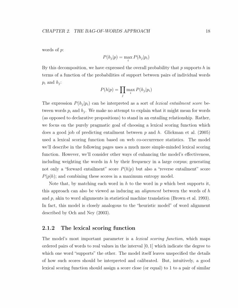
The expression P (hj|pi) can be interpreted as a sort of lexical entailment score be-tween words pi and hj. We make no attempt to explain what it might mean for words(as opposed to declarative propositions) to stand in an entailing relationship. Rather,we focus on the purely pragmatic goal of choosing a lexical scoring function whichdoes a good job of predicting entailment between p and h. Glickman et al. (2005)used a lexical scoring function based on web co-occurrence statistics. The modelwe’ll describe in the following pages uses a much more simple-minded lexical scoringfunction. However, we’ll consider other ways of enhancing the model’s effectiveness,including weighting the words in h by their frequency in a large corpus; generatingnot only a “forward entailment” score P (h|p) but also a “reverse entailment” scoreP (p|h); and combining these scores in a maximum entropy model.
Note that, by matching each word in h to the word in p which best supports it,this approach can also be viewed as inducing an alignment between the words of hand p, akin to word alignments in statistical machine translation (Brown et al. 1993).In fact, this model is closely analogous to the “heuristic model” of word alignmentdescribed by Och and Ney (2003).
2.1.2 The lexical scoring function
The model’s most important parameter is a lexical scoring function, which mapsordered pairs of words to real values in the interval [0, 1] which indicate the degree towhich one word “supports” the other. The model itself leaves unspecified the detailsof how such scores should be interpreted and calibrated. But, intuitively, a goodlexical scoring function should assign a score close (or equal) to 1 to a pair of similar

CHAPTER 2. THE BAG-OF-WORDS APPROACH 19
(or identical) words, and will assign a score close to 0 to a pair of dissimilar words.The best candidates for lexical scoring functions will therefore be measures of
lexical similarity, or perhaps the somewhat weaker notion of lexical relatedness. Can-didate scoring functions might include:
• measures of string similarity• similarity functions based on vector-space models, such as latent semantic anal-
ysis (LSA) (Landauer and Dumais 1997)• measures of distributional similarity, like that proposed by Lin (1998)• taxonomy-based scoring functions, such as one based on the WordNet-based
semantic distance measure of Jiang and Conrath (1997)
Alternatively, a lexical scoring function might be designed as a hybrid, whichcombines information from several component scoring functions. One advantage ofa hybrid scoring function is that it can incorporate information from low-coverage,high-precision scoring functions (for example, lexical resources providing informationabout acronyms) which would be inappropriate for use by themselves. However, thedesign of a hybrid scoring function presents several problems. How should the com-ponent scores be combined: via the max function, or perhaps as a weighted average?Another difficulty is that the component functions may produce very different dis-tributions of scores, particularly if some are designed as low-recall, high-precisionmeasures (e.g., acronym resources), while others are designed as high-recall, low-precision measures (e.g., distributional similarity). How do we define and implementa suitable calibration of scores between such component functions, so that scores fromdifferent component functions can meaningfully be compared?
Note that while many lexical scoring functions will be symmetric, this is notstrictly required. For example, if we have access to a lexical resource contain-ing hyponymy relations (such as WordNet (Fellbaum et al. 1998)), we may wishto define a scoring function which assigns a high score to hyponym pairs (such as〈mammal, horse〉) but not to hypernym pairs (such as 〈horse,mammal〉).
While the selection (or design) of a lexical scoring function presents many difficultchoices, in this chapter we’ll sidestep this complexity. Instead, we’ll develop a model

CHAPTER 2. THE BAG-OF-WORDS APPROACH 20
based on an extremely simple-minded lexical scoring function. Our lemma stringsimilarity function computes a lexical similarity score based on the Levenshtein stringedit distance (Levenshtein 1966) between the lemmas (base forms) of the input words.In order to achieve the appropriate normalization, we divide the edit distance by themaximum of the length of the two lemmas, and subtract the result from 1:
sim(w1, w2) = 1− dist(lemma(w1), lemma(w2))
max(|lemma(w1)|, |lemma(w2)|)
(Here lemma(w) denotes the lemma of word w; dist() denotes Levenshtein string editdistance; and | · | denotes string length.)
2.1.3 Per-word alignment costs
In the following discussion, it will be convenient to work in terms of costs, rather thanscores. Given our lexical scoring function sim, we can define a lexical cost function,which expresses the cost of aligning hypothesis word hj with premise word pi as thenegative logarithm of their similarity score:
cost(hj, pi) = − log sim(hj, pi)
The cost function has range [0,∞]: aligning equal words will have cost 0; aligningvery different words will have very high cost. And, of course, if sim is symmetric,then cost will be symmetric as well.
Following the approach described in section 2.1.1, the cost of aligning a givenhypothesis word hj to the premise p will be the minimum of the costs of aligning hjto each possible premise word pi:
cost(hj|p) = minicost(hj, pi)
(Note that cost(hj|p) is asymmetric, even if cost(hj, pi) is symmetric—this is thereason for the conditioning bar.)
We can improve robustness by putting an arbitrary upper bound, maxcost, on

CHAPTER 2. THE BAG-OF-WORDS APPROACH 21
word alignment costs; otherwise, a single hard-to-align hypothesis word can com-pletely block inference.
cost(hj|p) = min(maxcost,minicost(hj, pi))
Lower values formaxcostmake the model “looser”: since every word can be alignedmore cheaply, we’re more likely to predict equivalence between the premise and thehypothesis. Conversely, higher values for maxcost make the model “stricter”. Oneinterpretation of maxcost is that it represents the cost of inserting a word into h
which doesn’t correspond to anything in p.
2.1.4 Total alignment costs
The overall cost of aligning h to p can now be computed as the sum of the costs ofaligning the individual words in h.
cost(h|p) =∑j
cost(hj|p) =∑j
min(maxcost,minicost(hj, pi))
However, intuition suggests that we would like to be able to treat some wordsin h as more important than others. It is of no great consequence if we are unablecheaply to align small function words (such as the, for, or as) in h; it matters muchmore whether we can find a suitable alignment for big, rare words (such as Ahmadine-jad). To capture this intuition, we can define a weight function which represents theimportance of each word in alignment as a non-negative real value. We then definethe total cost of aligning h to p to be the weighted sum of the costs of aligning theindividual words in h:
cost(h|p) =∑j
weight(hj) · cost(hj|p)
Just as there were many possible choices for the lexical scoring function, we havemany possible choices for this lexical weight function weight(hj). Clearly, we wantcommon words to receive less weight, and rare words to receive higher weight. A

CHAPTER 2. THE BAG-OF-WORDS APPROACH 22
plausible weight function might also take account of the part of speech of each word.However, to keep things simple, we’ll use a weight function based on the inversedocument frequency (IDF) of each word in a large corpus. If N is the number ofdocuments in our corpus and Nw is the number of documents containing word w,then we define:
idf(w) = − log(Nw/N)
Since the value of this function will be infinite for words which do not appear in thecorpus, we’ll define our weight function to place an upper bound on weights. We’llscale IDF scores into the range [0, 1] by dividing each score by the highest scoreobserved in the corpus (typically, this is the score of words observed exactly once),and we’ll assign weight 1 to words not observed in the corpus. If W is the set ofwords observed in the corpus, then we define the weight function by:
weight(hj) = min
[1,
idf(hj)
maxw∈W idf(w)
]For example, when based on a typical corpus (the English Gigaword corpus), thisfunction assigns weight 0.0004 to the, 0.1943 to once, 0.6027 to transparent, and1.000 to Ahmadinejad.
2.1.5 Predicting entailment
Let’s return to our top-level concern: how do we predict whether an inference fromp to h is valid? Now that we have defined the function cost(h|p) expressing thecost of aligning h to p, we have two possible avenues. The first is to use cost(h|p)directly, following the approach described in section 2.1.1, to assign a probability tothe entailment from p to h:
P (h|p) = exp(−cost(h|p))
However, this method is rather inflexible: it utilizes only one measure of the overlapbetween p and h, and provides no automatic way to tune the threshold above which

CHAPTER 2. THE BAG-OF-WORDS APPROACH 23
to predict entailment.The second is to use features based on our cost function as input to a machine
learning classifier. Rather than using cost(h|p) directly to predict entailment, weconstruct a feature representation of the entailment problem using quantities derivedfrom the cost function, and train a statistical classifier to predict entailment usingthese feature representations as input. For this purpose, we used a simple maximumentropy (logistic regression) classifier with Gaussian regularization (and regularizationparameter σ = 1).
One advantage of this approach is that it enables us automatically to determine theappropriate threshold beyond which to predict entailment. Another is that it allowsus to combine different kinds of information about the similarity between p and h. Forexample, our feature representation can include not only the cost of aligning h to p,but also the reverse, that is, the cost of aligning p to h. (If p and h are nearly identical,then both cost(h|p) and cost(p|h) should be low; whereas if p subsumes h but alsoincludes extraneous content—a common situation in NLI problems—then cost(h|p)should be low, but cost(p|h) should be high.) We experimented with a number ofdifferent features based on the cost function, shown in figure 2.1. Intuitively, feqScoreis intended to represent the likelihood that p entails h; reqScore, that h entails p;eqvScore, that p and h are mutually entailing (i.e., equivalent); fwdScore, that pentails h and not vice-versa; revScore, that h entails p and not vice-versa; andindScore, that neither p and h entails the other (i.e., they are independent). However,these interpretations are merely suggestive—one of the virtues of the machine learningapproach is that a (suitably regularized) classifier can learn to exploit whicheverfeatures carry signal, and ignore the rest, whether or not the features well capturethe intended interpretations.
Clearly, there is considerable redundancy between these features, but becausemaximum entropy classifiers (unlike, say, Naïve Bayes classifiers) handle correlatedfeatures gracefully, this is not a source of concern. However, in experiments, we foundlittle benefit to including all of these features; using just the feqScore and reqScore
features gave results roughly as good as including any additional features.

CHAPTER 2. THE BAG-OF-WORDS APPROACH 24
hCost = cost(h|p)pCost = cost(p|h)
feqScore = exp(−hCost)
reqScore = exp(−pCost)
eqvScore = feqScore · reqScorefwdScore = feqScore · (1− reqScore)
revScore = (1− feqScore) · reqScoreindScore = (1− feqScore) · (1− reqScore)
Figure 2.1: Possible features for a maximum-entropy model entailment based on thebag-of-words model.
2.2 Experimental results
Despite its simplicity, the bag-of-words model described in section 2.1 yields re-spectable performance when applied to real NLI problems such as those in the RTEtest suites. In order to establish a baseline against which to compare results in laterchapters, we performed experiments designed to quantify the effectiveness of the bag-of-words approach. In particular, we used the simple lemma string similarity functiondescribed in section 2.1.2 as our lexical scoring function; we placed an upper bound of10 on per-word alignment costs, as described in section 2.1.3; we combined per-wordalignment costs using IDF weighting, as described in section 2.1.4; and we made en-tailment predictions using a maximum-entropy classifier with Gaussian regularization,using only the features feqScore and reqScore, as described in section 2.1.5.
Table 2.1 shows the results of evaluating this model on various combinations oftraining and testing data from the RTE test suites. For comparison, table 2.2 showsresults from teams participating in the first three RTE competitions. The figures leadus to a number of surprising observations.
First, the bag-of-words model performs unexpectedly well, especially in light ofthe fact that it is based on a simple-minded measure of string similarity. While itis not competitive with the best RTE systems, it achieves an accuracy comparable

CHAPTER 2. THE BAG-OF-WORDS APPROACH 25
Training data Test data % yes P % R % Acc %
RTE1 dev RTE1 dev 49.7 53.9 53.7 54.0RTE1 test 50.1 53.6 53.8 53.6
RTE2 dev RTE2 dev 52.2 56.7 59.2 57.0RTE2 test 52.4 57.3 60.0 57.6
RTE3 dev RTE3 dev 50.6 70.1 68.9 68.9RTE3 test 57.5 62.4 70.0 63.0
RTE3 test RTE3 dev 46.9 71.2 64.8 68.4RTE3 test 53.8 63.0 66.1 62.8
Table 2.1: Performance of the bag-of-words entailment model described in section 2.1on various combinations of RTE training and test data (two-way classification). Thecolumns show the training data used, the test data used, the proportion of yespredictions, precision and recall for the yes class, and accuracy.
Evaluation System Acc %
RTE1 test Best: Glickman et al. 05 58.6Average (13 teams) 54.8Median (13 teams) 55.9
RTE2 test Best: Hickl et al. 06 75.4Average (23 teams) 59.8Median (23 teams) 59.0
RTE3 test Best: Hickl et al. 07 80.0Average (26 teams) 62.4Median (26 teams) 62.6
Table 2.2: Results from teams participating in the first three RTE competitions. Foreach RTE competition, we show the accuracy achieved by the best-performing team,along with average and median accuracies over all participating teams. Each RTEcompetition allowed teams to submit two runs; for those teams which did so, we usedthe run with higher accuracy in computing all statistics.

CHAPTER 2. THE BAG-OF-WORDS APPROACH 26
to the average and median accuracies achieved by all RTE participants in each ofthe RTE competitions. Indeed, when evaluated on the RTE3 test set (after trainingon the RTE3 development set), the bag-of-words model achieved an accuracy (63%)higher than that of more than half of the RTE3 participants. Many of those teamshad pursued approaches which were apparently far more sophisticated than the bag-of-words model, yet our results show that they could have done better with a morenaïve approach.
Note that, while the system of Glickman et al. (2005) was essentially a pure bag-of-words model, few or none of the systems submitted to RTE2 or RTE3 could bedescribed as such. Most of those which came closest to measuring pure lexical overlap(e.g., Adams (2006), Malakasiotis and Androutsopoulos (2007)) exploited additionalinformation as well, such as the occurrence of negation in p or h. For comparison,Zanzotto et al. (2006) describe experiments using a simple statistical lexical system,similar to the one described in this chapter. They were able to achieve accuracy closeto 60% on both RTE1 and RTE2, and found that simple lexical models outperformedmore sophisticated lexical models, thus confirming our findings.
The second surprise in table 2.1 is the degree of variance in the results acrossdata sets. A long-standing criticism of the RTE test suites has been that, becausethe task is loosely defined and the problems are not drawn from any “natural” datadistribution, there is no way to ensure consistency in the nature and difficulty of theNLI problems from one RTE data set to the next. Many in the RTE community havethe subjective perception that the character of the problems has changed significantlyfrom one RTE test suite to the next; the results in table 2.1 show that there aresubstantial objective differences as well. Using our simple bag-of-words model as ayardstick, the RTE1 test suite is the hardest, while the RTE2 test suite is roughly 4%easier, and the RTE3 test suite is roughly 9% easier. Moreover, in RTE3 there is amarked disparity between the difficulty of the development and test sets. Whicheverdata set we train on, the RTE3 development set appears to be roughly 6% easier thanthe RTE3 test set—certainly, an undesirable state of affairs.
A final observation about the results in table 2.1 is that the model does notappear to be especially prone to overfitting. Half of the rows in table 2.1 show

CHAPTER 2. THE BAG-OF-WORDS APPROACH 27
results for experiments where the test data is the same as the training data, yet theseresults are not appreciably better than the results for experiments where the testdata is different from the training data. However, this result is not too surprising—because the maximum entropy classifier uses just two features, it has only three freeparameters, and thus is unlikely to overfit the training data.

Chapter 3
Alignment for natural language
inference
In order to recognize that Kennedy was killed can be inferred from JFK was assassi-nated, one must first recognize the correspondence between Kennedy and JFK, andbetween killed and assassinated. Consequently, most current approaches to NLI rely,implicitly or explicitly, on a facility for alignment—that is, establishing links betweencorresponding entities and predicates in the premise p and the hypothesis h.
Recent entries in the annual Recognizing Textual Entailment (RTE) competition(Dagan et al. 2005) have addressed the alignment problem in a variety of ways, thoughoften without distinguishing it as a separate subproblem. Glickman et al. (2005)and Jijkoun and de Rijke (2005), among others, have explored approaches like thatpresented in chapter 2, based on measuring the degree of lexical overlap between bagsof words. While ignoring structure, such methods depend on matching each word in hto the word in p with which it is most similar—in effect, an alignment. At the otherextreme, Tatu and Moldovan (2007) and Bar-Haim et al. (2007) have formulatedthe inference problem as analogous to proof search, using inferential rules whichencode (among other things) knowledge of lexical relatedness. In such approaches,the correspondence between the words of p and h is implicit in the steps of the proof.
Increasingly, however, the most successful RTE systems have made the align-ment problem explicit. Marsi and Krahmer (2005) and MacCartney et al. (2006)
28

CHAPTER 3. ALIGNMENT FOR NATURAL LANGUAGE INFERENCE 29
first advocated pipelined system architectures containing a distinct alignment com-ponent, a strategy crucial to the top-performing systems of Hickl et al. (2006) andHickl and Bensley (2007). However, each of these systems has pursued alignmentin idiosyncratic and poorly-documented ways, often using proprietary data, makingcomparisons and further development difficult.
In this chapter we undertake the first systematic study of alignment for NLI.1 Wepropose a new NLI alignment system (the MANLI system) which uses a phrase-basedrepresentation of alignment, exploits external resources for knowledge of semanticrelatedness, and capitalizes on the recent appearance of new supervised training datafor NLI alignment. In addition, we examine the relation between alignment for NLIand alignment for machine translation (MT), and investigate whether existing MTaligners can usefully be applied in the NLI setting.
3.1 NLI alignment vs. MT alignment
The alignment problem is familiar in MT, where recognizing that she came is a goodtranslation for elle est venue requires establishing a correspondence between she andelle, and between came and est venue. The MT community has developed not onlyan extensive literature on alignment (Brown et al. 1993, Vogel et al. 1996, Marcuand Wong 2002, DeNero et al. 2006), but also standard, proven alignment tools suchas GIZA++ (Och and Ney 2003). Can off-the-shelf MT aligners be applied to NLI?There is reason to be doubtful. Alignment for NLI differs from alignment for MT inseveral important respects, including:
• Most obviously, it is monolingual rather than cross-lingual, opening the doorto utilizing abundant (monolingual) sources of information on semantic relat-edness, such as WordNet.
• It is intrinsically asymmetric: p is often much longer than h, and commonlycontains phrases or clauses which have no counterpart in h.
1The material in this chapter is derived in large part from (MacCartney et al. 2008).

CHAPTER 3. ALIGNMENT FOR NATURAL LANGUAGE INFERENCE 30
• Indeed, one cannot assume even approximate semantic equivalence—usually agiven in MT. Because NLI problems include both valid and invalid inferences,the semantic content of h may diverge substantially from p. An NLI alignermust be designed to accommodate frequent unaligned words and phrases.
• Little training data is available. MT alignment models are typically trainedin unsupervised fashion, inducing lexical correspondences from massive quan-tities of sentence-aligned bitexts. While NLI aligners could in principle do thesame, large volumes of suitable data are lacking. NLI aligners must thereforedepend on smaller quantities of supervised training data, supplemented by ex-ternal lexical resources. Conversely, while existing MT aligners can make use ofdictionaries, they are not designed to harness other sources of information ondegrees of semantic relatedness.
Consequently, the tools and techniques of MT alignment may not transfer readily toNLI alignment. We investigate the matter empirically in section 3.4.2.
3.2 The MSR alignment data
Until recently, research on alignment for NLI has been hampered by a paucity ofhigh-quality, publicly available data from which to learn. Happily, that has begunto change, with the release by Microsoft Research (MSR) of gold-standard alignmentannotations (Brockett 2007) for inference problems from the second Recognizing Tex-tual Entailment (RTE2) challenge (Bar-Haim et al. 2006). To our knowledge, we arethe first to exploit this data for training and evaluation of NLI alignment models.
The RTE2 data consists of a development set and a test set, each containing800 inference problems. Each problem consists of a premise p and a hypothesis h.The premises contain 29 words on average; the hypotheses, 11 words. Each problemis marked as a valid or invalid inference (50% each); however, these annotationsare ignored during alignment, since they would not be available during testing of acomplete NLI system.

CHAPTER 3. ALIGNMENT FOR NATURAL LANGUAGE INFERENCE 31
In
most
Pacific
countries
there
are
very
few
women
in
parliament
.
Women
arepoorly
represented
in parliament
.
Figure 3.1: The MSR gold standard alignment for problem 116 from the RTE2 de-velopment set.
The MSR annotations use an alignment representation which is token-based, butmany-to-many, and thus allows implicit alignment of multi-word phrases. Figure 3.1shows an example in which very few has been aligned with poorly represented.
In the MSR data, every alignment link is marked as sure or possible. In makingthis distinction, the annotators have followed a convention common in MT, whichpermits alignment precision to be measured against both sure and possible links,while recall is measured against only sure links. In this work, however, we havechosen to ignore possible links, embracing the argument made by Fraser and Marcu(2007) that their use has impeded progress in MT alignment models, and that sure-only annotation is to be preferred.
Each RTE2 problem was independently annotated by three people, following care-fully designed annotation guidelines. Inter-annotator agreement was high: Brockett(2007) reports Fleiss’ kappa2 scores of about 0.73 (“substantial agreement”) for map-pings from h tokens to p tokens; and all three annotators agreed on ∼70% of proposed
2Fleiss’ kappa generalizes Cohen’s kappa to the case where there are more than two raters.

CHAPTER 3. ALIGNMENT FOR NATURAL LANGUAGE INFERENCE 32
links, while at least two of three agreed on more than 99.7% of proposed links,3 at-testing to the high quality of the annotation data. For this work, we merged the threeindependent annotations, according to majority rule,4 to obtain a gold-standard an-notation containing an average of 7.3 links per RTE problem.
3.3 The MANLI aligner
In this section, we describe the MANLI aligner, a new alignment system designedexpressly for NLI alignment. The MANLI system consists of four elements:
• a phrase-based representation of alignment,
• a feature-based linear scoring function for alignments,
• a decoder which uses simulated annealing to find high-scoring alignments, and
• perceptron learning to optimize feature weights.
In the following pages, we’ll describe each of these elements in turn.
3.3.1 A phrase-based alignment representation
MANLI uses an alignment representation which is intrinsically phrase-based. (Fol-lowing the usage common in MT, we use “phrase” to mean any contiguous span oftokens, not necessarily corresponding to a syntactic phrase.) We represent an align-ment E between a premise p and a hypothesis h as a set of phrase edits {e1, e2, . . .},each belonging to one of four types:
• an eq edit connects a phrase in p with an equal (by word lemmas) phrase in h
• a sub edit connects a phrase in p with an unequal phrase in h
• a del edit covers an unaligned phrase in p
• an ins edit covers an unaligned phrase in h

CHAPTER 3. ALIGNMENT FOR NATURAL LANGUAGE INFERENCE 33
del(In1)del(most2)del(Pacific3)del(countries4)del(there5)eq(are6, are2)sub(very7 few8, poorly3 represented4)eq(women9, Women1)eq(in10, in5)eq(parliament11, parliament6)eq(.12, .7)
Figure 3.2: The MSR gold standard alignment for RTE2 problem 116 (the sameproblem as in figure 3.1), represented as a set of phrase edits. Note that del and insedits of size > 1 are possible in principle, but are not used in our training data.
As an example, figure 3.2 shows the same alignment as in figure 3.1, but representedas a set of phrase edits.
Alignments are constrained to be one-to-one at the phrase level: every token in pand h belongs to exactly one phrase, which participates in exactly one edit (possiblydel or ins). However, the phrase representation permits alignments which are many-to-many at the token level. In fact, this is the chief motivation for the phrase-basedrepresentation: we can align very few and poorly represented as units, without beingforced to make an arbitrary choice as to which word goes with which word. Moreover,our scoring function can make use of lexical resources which have information aboutsemantic relatedness of multi-word phrases, not merely individual words.
About 23% of the MSR gold-standard alignments are not one-to-one (at the tokenlevel), and are therefore technically unreachable for MANLI, which is constrained togenerate one-to-one alignments. However, by merging contiguous token links intophrase edits of size > 1, most MSR alignments (about 92%) can be straightforwardlyconverted into MANLI-reachable alignments. For the purpose of model training (butnot for the evaluation described in section 3.4.4), we generated a version of the MSR
3The sure/possible distinction is taken as significant in computing all these figures.4The handful of three-way disagreements were treated as possible links, and thus were not used.

CHAPTER 3. ALIGNMENT FOR NATURAL LANGUAGE INFERENCE 34
data in which all alignments were converted to MANLI-reachable form.5
3.3.2 A feature-based scoring function
To score alignments, we use a simple feature-based linear scoring function, in whichthe score of an alignment is the sum of the scores of the edits it contains (includingnot only sub and eq edits, but also del and ins edits), and the score of an edit isthe dot product of a vector encoding its features and a vector of weights. If E is a setof edits constituting an alignment, and Φ is a vector of feature functions, the score sis given by:
s(E) =∑e∈E
s(e) =∑e∈E
w ·Φ(e)
We’ll explain how the feature weights w are set in section 3.3.4. The features usedto characterize each edit are as follows:
Edit type features. We begin with boolean features encoding the type of eachedit. We expect eqs to score higher than subs, and (since p is commonly longer thanh) dels to score higher than inss.
Phrase features. Next, we have features which encode the sizes of the phrasesinvolved in the edit, and whether these phrases are non-constituents (in syntacticparses of the sentences involved).
Semantic relatedness feature. For sub edits, a very important feature representsthe degree of semantic relatedness of the substituends, as a real value in [0, 1]. Thisrelatedness score is computed as a max over a number of component scoring functions,some based on external lexical resources, including:
• various string similarity functions, of which most are applied to word lemmas5About 8% of the MSR alignments contain non-contiguous links, most commonly because p
contains two references to an entity (e.g., Christian Democrats and CDU ) which are both linkedto a reference to the same entity in h (e.g., Christian Democratic Union). In such cases, one ormore links must be eliminated to achieve a MANLI-reachable alignment. We used a string-similarityheuristic to break such conflicts, but were obliged to make an arbitrary choice in about 2% of cases.

CHAPTER 3. ALIGNMENT FOR NATURAL LANGUAGE INFERENCE 35
• measures of synonymy, hypernymy, antonymy, and semantic relatedness, includ-ing a widely-used measure due to Jiang and Conrath (1997), based on manuallyconstructed lexical resources such as WordNet and NomBank
• a function based on the well-known distributional similarity metric of Lin (1998),which automatically infers similarity of words and phrases from their distribu-tions in a very large corpus of English text
The ability to leverage external lexical resources—both manually constructed andautomatically induced—is critical to the success of MANLI.
Contextual features. Even when the lexical similarity for a sub edit is high,it may not be a good match. If p or h contains multiple occurrences of the sameword—which happens frequently with function words, and occasionally with contentwords—lexical similarity alone may not suffice to determine which is the right match.To remedy this, we introduce contextual features for sub and eq edits. A real-valued distortion feature measures the difference between the relative positions ofthe substituends within their respective sentences, while boolean matching neighborsfeatures indicate whether the tokens before and after the substituends are equal orsimilar.
3.3.3 Decoding using simulated annealing
The problem of decoding—that is, finding a high-scoring alignment for a par-ticular inference problem—is made more complex by our choice of a phrase-basedalignment representation. For a model which uses a token-based representation (say,one which simply maps h tokens to p tokens), decoding is trivial, since each tokencan be aligned independently of its neighbors. (This is the case for the bag-of-wordsmodel described in chapter 2.) But with a phrase-based representation, things aremore complicated. The segmentation into phrases is not given in advance, and everyphrase pair considered for alignment must be consistent with its neighbors with re-spect to segmentation. Consequently, the decoding problem cannot be factored intoa number of independent decisions.
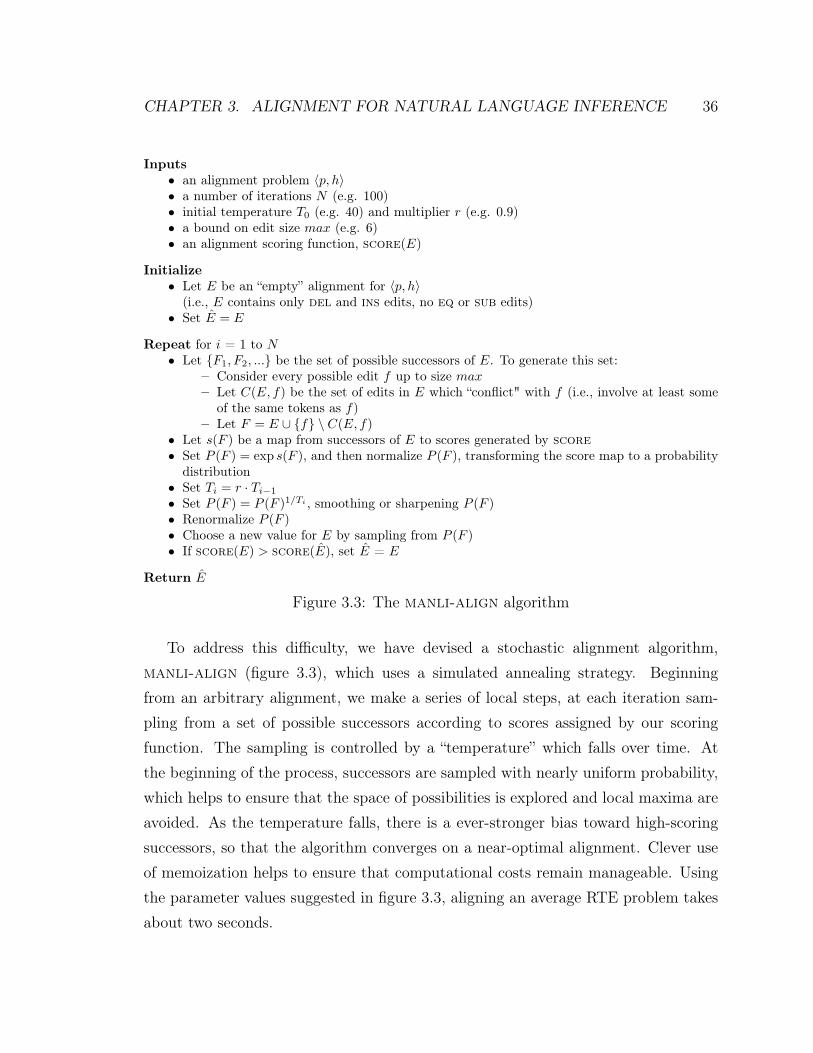
CHAPTER 3. ALIGNMENT FOR NATURAL LANGUAGE INFERENCE 36
Inputs• an alignment problem 〈p, h〉• a number of iterations N (e.g. 100)• initial temperature T0 (e.g. 40) and multiplier r (e.g. 0.9)• a bound on edit size max (e.g. 6)• an alignment scoring function, score(E)
Initialize• Let E be an “empty” alignment for 〈p, h〉
(i.e., E contains only del and ins edits, no eq or sub edits)• Set E = E
Repeat for i = 1 to N• Let {F1, F2, ...} be the set of possible successors of E. To generate this set:
– Consider every possible edit f up to size max– Let C(E, f) be the set of edits in E which “conflict" with f (i.e., involve at least some
of the same tokens as f)– Let F = E ∪ {f} \ C(E, f)
• Let s(F ) be a map from successors of E to scores generated by score• Set P (F ) = exp s(F ), and then normalize P (F ), transforming the score map to a probability
distribution• Set Ti = r · Ti−1
• Set P (F ) = P (F )1/Ti , smoothing or sharpening P (F )• Renormalize P (F )• Choose a new value for E by sampling from P (F )• If score(E) > score(E), set E = E
Return E
Figure 3.3: The manli-align algorithm
To address this difficulty, we have devised a stochastic alignment algorithm,manli-align (figure 3.3), which uses a simulated annealing strategy. Beginningfrom an arbitrary alignment, we make a series of local steps, at each iteration sam-pling from a set of possible successors according to scores assigned by our scoringfunction. The sampling is controlled by a “temperature” which falls over time. Atthe beginning of the process, successors are sampled with nearly uniform probability,which helps to ensure that the space of possibilities is explored and local maxima areavoided. As the temperature falls, there is a ever-stronger bias toward high-scoringsuccessors, so that the algorithm converges on a near-optimal alignment. Clever useof memoization helps to ensure that computational costs remain manageable. Usingthe parameter values suggested in figure 3.3, aligning an average RTE problem takesabout two seconds.

CHAPTER 3. ALIGNMENT FOR NATURAL LANGUAGE INFERENCE 37
Inputs• training problems 〈pj , hj〉, j = 1..n• corresponding gold-standard alignments Ej
• a number of learning epochs N (e.g. 50)• a “burn-in” period N0 < N (e.g. 10)• initial learning rate R0 (e.g. 1) and multiplier r (e.g. 0.8)• a vector of feature functions Φ(E)• an alignment algorithm align(p, h;w) which finds a good alignment for 〈p, h〉 using weight
vector w
Initialize• Set w = 0
Repeat for i = 1 to N• Set Ri = r ·Ri−1, reducing the learning rate• Randomly shuffle the training problems• For j = 1 to n:
– Set Ej = align(pj , hj ; w)– Set w = w + Ri · (Φ(Ej)−Φ(Ej))
• Set w = w/‖w‖2 (L2 normalization)• Set w[i] = w, storing the weight vector for this epoch
Return an averaged weight vector:• wavg = 1/(N −N0)
∑Ni=N0+1 w[i]
Figure 3.4: The manli-learn algorithm
While manli-align is not guaranteed to produce optimal alignments, there isreason to believe that it usually comes very close. After training, the alignmentfound by MANLI scored at least as high as the gold alignment for 99.6% of RTEproblems.6
3.3.4 Perceptron learning
To tune the parameters w of the model, we use an adaptation of the averagedperceptron algorithm (Collins 2002), which has proven successful on a range of NLPtasks. The algorithm is shown in figure 3.4. After initializing w to 0, we perform N
training epochs. (Our experiments used N = 50.) In each epoch, we iterate throughthe training data, updating the weight vector at each training example according to
6This figure is based on the MANLI-reachable version of the gold-standard data described insection 3.3.1. For the raw gold-standard data, the figure is 88.1%. The difference is almost entirelyattributable to unreachable gold alignments, which tend to score higher simply because they containmore edits (and because the learned weights are mostly positive).

CHAPTER 3. ALIGNMENT FOR NATURAL LANGUAGE INFERENCE 38
the difference between the features of the target alignment7 and the features of thealignment produced by the decoder using the current weight vector. The size of theupdate is controlled by a learning rate which decreases over time. At the end of eachepoch, the weight vector is normalized and stored. The final result is the averageof the stored weight vectors, omitting vectors from a fixed number of epochs at thebeginning of the run (which tend to be of poor quality). Using the parameter valuessuggested in figure 3.4, training runs on the RTE2 development set required about20 hours.
3.4 Evaluating aligners on MSR data
In this section, we describe experiments designed to evaluate the performance ofvarious alignment systems on the MSR gold-standard data described in section 3.2.For each system, we report precision, recall, and F-measure (F1). These statisticsare assessed per problem by counting aligned token pairs.8 In a particular alignmentproblem, if A is the set of token pairs which are aligned in the guessed alignment,and S is the set of token pairs which are aligned in the gold alignment, then precisionP = |A ∩ S|/|A|, while recall R = |A ∩ S|/|S|. F-measure is defined as usual byF1 = 2PR/(P +R).9 P , R, and F1 are then averaged over all problems in a problemset.10 We also report the exact match rate: that is, the proportion of problems inwhich the guessed alignment exactly matches the gold alignment. The results aresummarized in table 3.1.
7For training (but not for testing), we produced a version of the gold-standard data in whichcontiguous many-to-many token links (as in figure 3.1) were merged into sub edits of size > 1 (anda few non-contiguous links were eliminated).
8For phrase-based alignments like those generated by MANLI, two tokens are considered to bealigned iff they are contained within phrases which are aligned.
9MT researchers conventionally report results in terms of alignment error rate (AER). Since weuse only sure links in the gold standard data (see section 3.2), AER is equivalent to 1− F1.
10Note that this is a form of macro-averaging. MT evaluations conventionally use micro-averaging,which gives greater weight to problems containing more aligned pairs. This makes sense in MT,where the purpose of alignment is to induce phrase tables. But in NLI, where the ultimate goal is tomaximize the number of inference problems answered correctly, it is more fitting to give all problemsequal weight, and so we macro-average. We have also generated all results using micro-averaging,and found that the relative comparisons are not greatly affected.

CHAPTER 3. ALIGNMENT FOR NATURAL LANGUAGE INFERENCE 39
3.4.1 A robust baseline: the bag-of-words aligner
As a baseline, we use a simple alignment algorithm which is essential the same asthe bag-of-words model presented in chapter 2. Each hypothesis token hj is alignedto the premise token pi to which it is most similar, according to a lexical similarityfunction based on string edit distance between word lemmas. To generate alignmentscores (which will be of interest in section 3.5), we simply normalize the cost functiondefined in section 2.1.4 by the length of h:
score(h|p) =1
|h|cost(h|p)
Despite the simplicity of this alignment model, its performance is fairly robust, withgood recall. Its precision, however, its mediocre—chiefly because, by design, it alignsevery hypothesis token with some premise token. The model could surely be improvedby allowing it to leave some h tokens unaligned, but this was not pursued.
3.4.2 MT aligners: GIZA++ and Cross-EM
Given the importance of alignment for NLI, and the availability of standard, proventools for MT alignment, an obvious question presents itself: why not use an off-the-shelf MT aligner for NLI? Although we have argued (section 3.1) that this is unlikelyto succeed, to our knowledge, we are the first to investigate the matter empirically.11
The best-known and most-used MT aligner is undoubtedly GIZA++ (Och andNey 2003), which contains implementations of various IBM models (Brown et al.1993), as well as the HMM model of Vogel et al. (1996). Most practitioners useGIZA++ as a black box, via the Moses MT toolkit (Koehn et al. 2007). We fol-lowed this practice, running with Moses’ default parameters on the RTE2 data toobtain asymmetric word alignments in both directions (p-to-h and h-to-p). We thenperformed symmetrization using the well-known intersection heuristic.
Unsurprisingly, the out-of-the-box performance was quite poor, with most wordsaligned apparently at random. Precision was fair (72%) but recall was very poor
11However, Dolan et al. (2004) explore a closely-related topic: using an MT aligner to identifyparaphrases.

CHAPTER 3. ALIGNMENT FOR NATURAL LANGUAGE INFERENCE 40
System Data P % R % F1 % E %
Bag-of-words dev 57.8 81.2 67.5 3.5(baseline) test 62.1 82.6 70.9 5.3GIZA++ dev 83.0 66.4 72.1 —(using lexicon, ∩ heuristic) test 85.1 69.1 74.8 —Cross-EM dev 67.6 80.1 72.1 —(using lexicon, ∩ heuristic) test 70.3 81.0 74.1 —Stanford RTE dev 81.1 61.2 69.7 0.5
test 82.7 61.2 70.3 0.3Stanford RTE dev 81.1 75.8 78.4 —(punctuation correction) test 82.7 75.8 79.1 —MANLI dev 83.4 85.5 84.4 21.7
test 85.4 85.3 85.3 21.3
Table 3.1: Performance of various aligners on the MSR RTE2 alignment data. Thecolumns show the data set used (800 problems each); average precision, recall, andF-measure; and the exact match rate (see text).
(46%). Even equal words were usually not aligned—because GIZA++ is designedfor cross-linguistic use, it does not consider word equality between source and tar-get sentences. To remedy this, we supplied GIZA++ with a lexicon, using a trickcommon in the MT community: we supplemented the training data with syntheticdata consisting of matched pairs of equal words. This gives GIZA++ a better chanceof learning that, e.g., man should align with man. The result was a big boost inrecall (+23%), and a smaller gain in precision. The results for GIZA++ shown intable 3.1 are based on using the lexicon and intersection. With these settings,GIZA++ properly aligned most pairs of equal words, but continued to align otherwords apparently at random.
Next, we compared the performance of intersection with other symmetriza-tion heuristics defined in Moses—including union, grow, grow-diag, grow-diag-
final (the default), and grow-diag-final-and—and with asymmetric alignments

CHAPTER 3. ALIGNMENT FOR NATURAL LANGUAGE INFERENCE 41
in both directions. While all these alternatives achieved better recall than inter-
section, all showed substantially worse precision and F1. On the RTE2 test set, theasymmetric alignment from h to p scored 68% in F1; grow scored 58%; and all otheralternatives scored below 52%.
As an additional experiment, we tested the Cross-EM aligner (Liang et al. 2006)from the BerkeleyAligner package on the MSR data. While this aligner is in manyways simpler than GIZA++ (it lacks any model of fertility, for example), its methodof jointly training two simple asymmetric HMM models has outperformed GIZA++on standard evaluations of MT alignment. As with GIZA++, we experimented witha variety of symmetrization heuristics, and ran trials with and without a supplemen-tal lexicon. The results were broadly similar: intersection greatly outperformedalternative heuristics, and using a lexicon provided a big boost (up to 12% in F1).Under optimal settings, the Cross-EM aligner showed better recall and worse preci-sion than GIZA++, with F1 just slightly lower. Like GIZA++, it did well at aligningequal words, but aligned most other words at random.
The mediocre performance of MT aligners on NLI alignment comes as no surprise,for reasons discussed in section 3.1. Above all, the quantity of training data is simplytoo small for unsupervised learning to succeed. A successful NLI aligner will needto exploit supervised training data, and will need access to additional sources ofknowledge about lexical relatedness.
3.4.3 The Stanford RTE aligner
A better comparison is thus to an alignment system expressly designed for NLI. Forthis purpose, we used the alignment component of the Stanford RTE system, whichwill be described in chapter 4.12 The Stanford aligner performs decoding and learningin a similar fashion to MANLI, but uses a simpler, token-based alignment representa-tion, along with a richer set of features for alignment scoring. It represents alignmentsas an injective map from h tokens to p tokens. Phrase alignments are not directlyrepresentable, although the effect can be approximated by a pre-processing step which
12However, the experiments described here used a more recent version of the Stanford RTE system(best described in (Chambers et al. 2007)) than that which forms the basis of chapter 4.

CHAPTER 3. ALIGNMENT FOR NATURAL LANGUAGE INFERENCE 42
collapses multi-token named entities and certain collocations into single tokens. Thefeatures used for alignment scoring include not only measures of lexical similarity, butalso syntactic features encoding the similarity of paths through dependency parsesbetween pairs of aligned tokens, which are intended to promote the alignment ofsimilar predicate-argument structures.
Despite this sophistication, the out-of-the-box performance of the Stanford aligneris mediocre, as shown in table 3.1. The low recall figures are particularly notewor-thy. However, a partial explanation is readily available: by design, the Stanfordsystem ignores punctuation.13 Because punctuation tokens constitute about 15% ofthe aligned pairs in the MSR data, this sharply reduces measured recall. However,since punctuation matters little in inference, such recall errors arguably should beforgiven. Thus, table 3.1 also shows adjusted statistics for the Stanford system inwhich all punctuation alignments are (generously) counted as correct.
Even after this adjustment, the recall figures are unimpressive. Error analysisreveals that the Stanford aligner does a poor job of aligning function words. About13% of the aligned pairs in the MSR data are matching prepositions or articles; theStanford aligner misses about 67% of such pairs. (By contrast, MANLI misses only10% of such pairs.) While function words matter less in inference than nouns andverbs, they are not irrelevant, and because sentences often contain multiple instancesof a particular function word, matching them properly is by no means trivial. Ifmatching prepositions and articles were ignored (in addition to punctuation), the gapin F1 between the MANLI and Stanford systems would narrow to about 2.8%.
Finally, the Stanford aligner is handicapped by its token-based alignment repre-sentation, often failing (partly or completely) to align multi-word phrases such aspeace activists with protesters, or hackers with non-authorized personnel.
3.4.4 The MANLI aligner
As table 3.1 indicates, the MANLI aligner was found to outperform all other alignersevaluated on every measure of performance, achieving an F1 score 10.5% higher than
13In fact, it operates on a dependency-graph representation from which punctuation is omitted.

CHAPTER 3. ALIGNMENT FOR NATURAL LANGUAGE INFERENCE 43
GIZA++ and 6.2% higher than the Stanford aligner (even with the punctuationcorrection).14 MANLI achieved a good balance between precision and recall, andmatched more than 20% of the gold-standard alignments exactly.
Three factors seem to have contributed most to MANLI’s success. First, MANLIis able to outperform the MT aligners principally because it is able to leverage lexicalresources to identify the similarity between pairs of words such as jail and prison,prevent and stop, or injured and wounded. Second, MANLI’s contextual features en-able it to do better than the Stanford aligner at matching function words, a weaknessof the Stanford aligner discussed in section 3.4.3. Third, MANLI gains a marginaladvantage because its phrase-based representation of alignment permits it to properlyalign phrase pairs such as death penalty and capital punishment.
However, the phrase-based representation contributed far less than we had hoped.Setting MANLI’s maximum phrase size to 1 (effectively, restricting it to token-basedalignments) caused F1 to fall by just 0.2%. We do not interpret this to mean thatphrase alignments are not useful—indeed, about 2.6% of the links in the gold-standarddata involve phrases of size > 1. Rather, we think it shows that we have failed tofully exploit the advantages of the phrase-based representation, chiefly because welack lexical resources providing good information on similarity of multi-word phrases.Even if we had such resources, however, the consequent gains might be modest.Recent work by de Marneffe et al. (2009) suggests that the role played by multi-word expressions in RTE is smaller than one might expect, and is largely restrictedto lexico-syntactic variations which can be captured by other means.
Error analysis suggests that there is ample room for improvement. A large pro-portion of recall errors (perhaps 40%) occur because the lexical similarity functionassigns too low a value to pairs of words or phrases which are clearly similar, such asconservation and protecting, server and computer networks, organization and agen-cies, or bone fragility and osteoporosis. Better exploitation of lexical resources couldhelp to reduce such errors. Another important category of recall errors (about 12%)result from the failure to identify one- and multi-word versions of the name of someentity, such as Lennon and John Lennon, or Nike Inc. and Nike. A special-purpose
14Reported results for MANLI are averages over 10 runs.

CHAPTER 3. ALIGNMENT FOR NATURAL LANGUAGE INFERENCE 44
similarity function could help here. Note, however, that about 10% of the recall errorsare unavoidable, given our choice of alignment representation, since they involve caseswhere the gold standard aligns one or more tokens on one side to a non-contiguousset of tokens on the other side.
Precision errors may be harder to reduce. These errors are dominated by caseswhere we mistakenly align two equal function words (49% of precision errors), twoforms of the verb to be (21%), two equal punctuation marks (7%), or two words orphrases of other types having equal lemmas (18%). Because such errors often occurbecause the aligner is forced to choose between nearly equivalent alternatives, theymay be difficult to eliminate. The remaining 5% of precision errors result mostly fromaligning words or phrases rightly judged to be highly similar, such as expanding andincreasing, labor and birth, figures and number, or 223,000 and 220,000.
3.5 Using alignment to predict RTE answers
In section 3.4, we evaluated the ability of aligners to recover gold-standard alignments.But since alignment is just one component of the NLI problem, we might also examinethe impact of different aligners on the ability to recognize valid inferences. If a high-scoring alignment indicates a close correspondence between h and p, does this alsoindicate a valid inference? As we will argue in chapter 4, there is more to inferentialvalidity than close lexical or structural correspondence: negations, antonymy, modals,non-factive and implicative verbs, and other linguistic constructs can affect validityin ways hard to capture in alignment. Nevertheless, alignment score can be a strongpredictor of inferential validity, and some NLI systems (e.g., that of Glickman et al.(2005)) rely entirely on some measure of alignment quality to predict validity.
If an aligner generates real-valued alignment scores, we can use the RTE data totest its ability to predict inferential validity with the following simple method. For agiven RTE problem, we predict yes (valid) if its alignment score15 exceeds a threshold
15For good results, it may be necessary to normalize the alignment score. Scores from MANLIwere normalized by the number of tokens in the problem. The Stanford aligner performs a similarnormalization internally.

CHAPTER 3. ALIGNMENT FOR NATURAL LANGUAGE INFERENCE 45
System data acc % avgP %
Bag-of-words aligner dev 61.3 61.5test 57.9 58.9
Stanford RTE aligner dev 63.1 64.9test 60.9 59.2
MANLI aligner dev 59.3 69.0(this work) test 60.3 61.0LCC (Hickl et al. 2006) test 75.4 80.8RTE2 entries (average) test 58.5 59.1
Table 3.2: Performance of various aligners and complete RTE systems in predictingRTE2 answers. The columns show the data set used, accuracy, and average precision(the recommended metric for RTE2).
τ , and no otherwise. We tune τ to maximize accuracy on the RTE2 developmentset, and then measure accuracy on the RTE2 test set using the same τ .
Table 3.2 shows results for several NLI aligners, along with some results for com-plete RTE systems, including the LCC system (the top performer at RTE2) and anaverage of all systems participating in RTE2. While none of the aligners rivals theperformance of the LCC system, all achieve respectable results, and the Stanfordand MANLI aligners outperform the average RTE2 entry. Thus, even if alignmentquality does not determine inferential validity, many NLI systems could be improvedby harnessing a well-designed NLI aligner.
3.6 Conclusion
While MT aligners succeed by unsupervised learning of word correspondences frommassive amounts of bitext, NLI aligners are forced to rely on smaller quantities ofsupervised training data. With the MANLI system, we have demonstrated how toovercome this lack of data by utilizing external lexical resources, and how to gainadditional power from a phrase-based representation of alignment.

Chapter 4
The Stanford RTE system
In this chapter, we describe the Stanford RTE system1 for natural language infer-ence, which represents an initial attempt to find a middle ground between, on theone hand, approaches to NLI based on lexical similarity, which are robust, but im-precise; and on the other, approaches based on full semantic interpretation, whichare precise, but brittle. Because full, accurate, open-domain natural language under-standing lies far beyond current capabilities, most early efforts in natural languageinference sought to extract the maximum mileage from quite limited semantic rep-resentations. Some (like the bag-of-words model described in chapter 2) used simplemeasures of semantic overlap, but over time, the more interesting work largely con-verged on a graph-alignment approach, operating on semantic graphs derived fromsyntactic dependency parses, and using a locally-decomposable alignment score as aproxy for strength of entailment. (Below, we argue that even approaches relying onweighted abduction may be seen in this light.) In this chapter, we highlight the fun-damental semantic limitations of this type of approach, and advocate a multi-stagearchitecture that addresses these limitations. The three key limitations are an as-sumption of monotonicity, an assumption of locality, and a confounding of alignment
1The Stanford RTE system has been developed over several years by a large team, including (inaddition to this author) Rajat Raina, Trond Grenager, Marie-Catherine de Marneffe, Anna Rafferty,Christopher D. Manning, and many others. The material in this chapter is derived in large partfrom (MacCartney et al. 2006), and therefore reflects an earlier stage of development of the StanfordRTE system. The more recent evolution of the system is described in (Chambers et al. 2007, Padóet al. 2008).
46

CHAPTER 4. THE STANFORD RTE SYSTEM 47
and evaluation of entailment.The system described in this chapter was developed around, and evaluated on, nat-
ural language inference problems from the PASCAL RTE1 data (Dagan et al. 2005),which includes a development set of 567 problems and a test set of 800 problems.Some example problems are shown in figure 4.1.
4.1 Approaching a robust semantics
In this section we try to give a unifying overview to recent work on robust nat-ural language inference, to present fundamental limitations of prominent methods,and then to outline our approach to resolving them. Until 2006, all robust naturallanguage inference systems of which we are aware employed a single-stage match-ing/proof process, differing mainly in the sophistication of the matching stage. Thesimplest approach is to base the entailment prediction on the degree of semantic over-lap between the premise p and hypothesis h using models based on bags-of-words,bags-of-n-grams, TF-IDF scores, or something similar (Jijkoun and de Rijke 2005).(The model presented in chapter 2 typifies this approach.) Such models are too im-poverished to be of much use, however. Semantic overlap is typically a symmetricrelation, whereas entailment is clearly not. Moreover, because overlap models do notaccount for syntactic or semantic structure, they are easily fooled by examples likeproblem 2081 in figure 4.1.
A more sophisticated approach is to formulate the entailment prediction as agraph matching problem (Haghighi et al. 2005, de Salvo Braz et al. 2005). In thisformulation, the input sentences p and h are represented as normalized syntacticdependency graphs (like the one shown in figure 4.2) and entailment is approximatedwith an alignment between the h graph and a portion of the corresponding p graph.Each possible alignment of the graphs has an associated score, and the score of thebest alignment is used as an approximation to the strength of the entailment: abetter-aligned hypothesis is assumed to be more likely to be entailed. To enableincremental search, alignment scores are usually factored as a combination of localterms, corresponding to the nodes and edges of the two graphs. Unfortunately, even

CHAPTER 4. THE STANFORD RTE SYSTEM 48
59 p Two Turkish engineers and an Afghan translator kidnapped in Decemberwere freed Friday.
h translator kidnapped in Iraq no
98 p Sharon warns Arafat could be targeted for assassination.h prime minister targeted for assassination no
152 p Twenty-five of the dead were members of the law enforcement agencies andthe rest of the 67 were civilians.
h 25 of the dead were civilians. no
231 p The memorandum noted the United Nations estimated that 2.5 million to3.5 million people died of AIDS last year.
h Over 2 million people died of AIDS last year. yes
971 p Mitsubishi Motors Corp.’s new vehicle sales in the US fell 46 percent in June.h Mitsubishi sales rose 46 percent. no
1806 p Vanunu, 49, was abducted by Israeli agents and convicted of treason in 1986after discussing his work as a mid-level Dimona technician with Britain’sSunday Times newspaper.
h Vanunu’s disclosures in 1968 led experts to conclude that Israel has a stock-pile of nuclear warheads. no
2081 p The main race track in Qatar is located in Shahaniya, on the Dukhan Road.h Qatar is located in Shahaniya. no
Figure 4.1: Illustrative examples from the RTE1 development set. For each problem,we show the ID number, the premise p and hypothesis h, and the correct answer.Though most of the problems shown have answer no, the RTE data sets are actuallybalanced between yes and no.

CHAPTER 4. THE STANFORD RTE SYSTEM 49
with factored scores, the problem of finding the best alignment of two graphs is NP-complete, so exact computation is intractable. Authors have proposed a variety ofapproximate search techniques. Haghighi et al. (2005) divide the search into twosteps: in the first step they consider node scores only, which relaxes the problem to aweighted bipartite graph matching that can be solved in polynomial time, and in thesecond step they add the edge scores and hillclimb the alignment via an approximatelocal search.
A third approach, exemplified by Moldovan et al. (2003) and Raina et al. (2005),is to turn the syntactic representation into a neo-Davidsonian-style quasi-logical form,and to perform weighted abductive theorem proving in the tradition of Hobbs et al.(1988). We argue, however, that this style of weighted resolution theorem proving isactually isomorphic to the graph matching approach. For example, a neo-Davidsonianrepresentation of the graph in figure 4.2 might correspond to the quasi-LF
rose(e1) ∧ nsubj (e1, x1) ∧ sales(x1) ∧ nn(x1, x2) ∧ Mitsubishi(x2) ∧dobj (e1, x3) ∧ percent(x3) ∧ num(x3, x4) ∧ 46 (x4)
There is a term corresponding to each node and arc, and the unit resolution steps atthe core of resolution theorem proving consider matching an individual node or arcof the hypothesis with something from the premise, just as in the graph-matchingapproach.2
Finally, a few efforts (Akhmatova 2005, Fowler et al. 2005, Bos and Markert2005a) have tried to translate sentences into formulas of first-order logic, in order totest logical entailment with a theorem prover. While in principle this approach doesnot suffer from the limitations we describe below, in practice it has not borne muchfruit. Because few problem sentences can be accurately translated to logical form,and because logical entailment is a strict standard, recall tends to be poor.
The simple graph matching formulation of the problem belies three important is-sues. First, the above systems assume monotonicity: if a good match is found with apart of the premise, other material in the premise is assumed not to affect the validity
2A possible difference is that with a good supply of additional linguistic and world knowledgeaxioms—as is present in Moldovan et al. (2003) but not Raina et al. (2005)—the theorem provermay generate intermediate forms in the proof, but, nevertheless, individual terms are resolved locallywithout reference to global context.

CHAPTER 4. THE STANFORD RTE SYSTEM 50
of the match. But many entailment decisions are non-monotonic in the node and edgescores. Consider variants on problem 98 in figure 4.1. Suppose the hypothesis wereArafat targeted for assassination. This would allow a perfect graph match or zero-cost weighted abductive proof, because the hypothesis is a subgraph of the premise.However, this would be incorrect, because it ignores the modal operator could. Infor-mation that changes the validity of a proof can also exist outside a matching clause.Consider the alternate premise Sharon denies Arafat is targeted for assassination.3
The second issue is the assumption of locality. Locality is needed to allow practicalsearch, but many entailment decisions rely on global features of the alignment, andthus do not naturally factor by nodes and edges. To take just one example, droppinga restrictive modifier preserves entailment in a positive context, but not in a negativeone. For example, Dogs barked loudly entails Dogs barked, but No dogs barked loudlydoes not entail No dogs barked. These more global phenomena cannot be modeledwith a factored alignment score.
The last issue arising in the graph matching approaches is the inherent difficultyin confounding alignment and entailment determination. The way to show that onegraph element does not follow from another is to make the cost of aligning them high.However, since we are embedded in a search for the lowest cost alignment, this willjust cause the system to choose an alternate alignment rather than recognizing a non-entailment. In problem 152 of figure 4.1, we would like the hypothesis to align withthe first part of the premise, to be able to prove that civilians are not members oflaw enforcement agencies and conclude that the hypothesis does not follow from thepremise. But a graph-matching system will to try to get non-entailment by makingthe matching cost between civilians and members of law enforcement agencies bevery high. However, the likely result of that is that the final part of the hypothesiswill align with were civilians at the end of the premise, assuming that we allow thealignment to “break” arcs.4 Under this candidate alignment, the lexical alignments areperfect, and the only imperfect alignment is the subject arc of were is mismatched in
3This is the same problem labeled and addressed as context in (Tatu and Moldovan 2005).4Robust systems need to allow matches with imperfect arc correspondence. For instance, given
Bill went to Lyons to study French farming practices, we would like to be able to conclude that Billstudied French farming despite the small structural mismatch.

CHAPTER 4. THE STANFORD RTE SYSTEM 51
the two. A robust inference guesser will still likely conclude that there is entailment.We propose that all three problems can be resolved in a multi-stage architecture,
where the alignment phase is followed by a separate phase of entailment determi-nation. Finding aligned content is naturally useful, and can be done by any searchprocedure. Compared to previous work, our approach to alignment emphasizes struc-tural correspondence, and downplays issues like polarity and quantity, which can beleft to a subsequent entailment decision. For example, our alignment scoring functionis designed to encourage antonym matches, and ignore the negation of verb pred-icates. The ideas clearly generalize to evaluating several alignments, but we havefound working with the one-best alignment to be adequate for the PASCAL RTEdata. Given a good alignment, the determination of entailment reduces to a simpleclassification decision. The classifier can use hand-tuned weights, or it can be trainedto minimize a relevant loss function using standard techniques from machine learning.The classifier is built over features designed to identify patterns of valid and invalidinference. For example, they can detect that it is okay to add a restrictive modifierif the passage has a universal quantifier (All the students got on the bus |= All themale students got on the bus), whereas this form of inference is not supported in or-dinary (upward-monotone) contexts. Because we already have a complete alignment,the classifier’s decision can be conditioned on arbitrary global features of the alignedgraphs, and it can detect inversions of monotonicity.
4.2 System
Our system has three stages: linguistic analysis, alignment, and entailment determi-nation. In the following pages, we describe each of these stages in turn.
4.2.1 Linguistic analysis
In the first stage of processing, our goal is to compute linguistic representations of thepremise and hypothesis that contain as much information as possible about their se-mantic content. We use typed dependency graphs, which contain a node for each word,

CHAPTER 4. THE STANFORD RTE SYSTEM 52
rose
sales
Mitsubishi
percent
46
nsubj dobj
nn num
Figure 4.2: A typed dependency graph for problem 971 of figure 4.1.
and labeled edges representing the grammatical relations between words. An exampleof a typed dependency graph for problem 971 of figure 4.1 is given in figure 4.2. Theadvantage of this representation is that it contains much of the information aboutthe entities and relations between them described by the sentence, while being easyto compute deterministically from a syntactic parse. The disadvantage is that it failsproperly to represent many semantic phenomena; particularly egregious is its inabilityto represent quantification and modality.
Our general approach is first to parse the input sentences, and then to converteach of the resulting phrase structure trees to a typed dependency graph. We use theStanford parser (Klein and Manning 2003), a statistical syntactic parser trained on thePenn TreeBank. To ensure correct parsing, we preprocess the sentences to collapsenamed entities and collocations into single tokens (by joining separate words withunderscores). Named entities are identified by the Stanford Named Entity Recognizer(Finkel et al. 2005), a CRF-based NER system similar to that described by McCallumand Li (2003), and collocations are derived from consecutive words pairs in WordNet(Fellbaum et al. 1998).
We convert the phrase structure trees to typed dependency graphs using a set ofdeterministic hand-coded rules, as described by de Marneffe et al. (2006). Heads ofthe constituents are first identified using the Collins rules (Collins 2003), modified toretrieve semantic heads. For each grammatical relation, we define patterns over thephrase structure tree using a language similar to the tgrep utility. Each pattern is

CHAPTER 4. THE STANFORD RTE SYSTEM 53
rose → fellsales → sales
Mitsubishi → Mitsubishi_Motors_Corp.percent → percent
46 → 46
score: −0.8962
Figure 4.3: A sample alignment for problem 971 of figure 4.1.
matched against each dependency in the tree, adding the most specific relation foundas the typed dependency. The nodes in the final graph are then annotated with theirassociated word, part-of-speech (given by the parser), lemma (given by a finite-statetransducer described by Minnen et al. (2001)) and named-entity tag (given by theNER tagger).
4.2.2 Alignment
The purpose of the second phase of processing is to find a good partial alignmentbetween the typed dependency graphs representing the premise p and the hypothesish. An alignment consists of a mapping from each node (word) in the h graph toa single node in the p graph, or to null.5 Not all words in the premise graph aremapped to, since typically the premise contains much more information than neededto support the hypothesis. Furthermore, we do not require that the alignment con-tains a mapping for all words in the hypothesis. Figure 4.3 shows an example of analignment for problem 971 of figure 4.1.
The space of alignments is large: there are O((m+1)n) possible alignments for a pgraph with m nodes and an h graph with n nodes. We define a measure of alignmentquality, and a procedure for identifying high scoring alignments. We choose a locallydecomposable scoring function, such that the score of an alignment is the sum of thelocal node and edge alignment scores. Unfortunately, there is no polynomial time
5The limitations of using one-to-one alignments are mitigated by the fact that many multiwordexpressions (e.g., named entities, noun compounds, multiword prepositions) have been collapsed intosingle nodes during linguistic analysis.

CHAPTER 4. THE STANFORD RTE SYSTEM 54
algorithm for finding the exact best alignment. Instead we use an incremental beamsearch, combined with a node ordering heuristic, to do approximate global searchin the space of possible alignments. We have experimented with several alternativesearch techniques, and found that the solution quality is not very sensitive to thespecific search procedure used.
Our scoring measure is designed to favor alignments which align semanticallysimilar subgraphs, irrespective of polarity. For this reason, nodes receive high align-ment scores when the words they represent are semantically similar. Synonyms andantonyms receive the highest score, and unrelated words receive the lowest. Ourhand-crafted scoring metric takes into account the word, the lemma, and the part ofspeech, and searches for word relatedness using a range of external resources, includ-ing WordNet, precomputed latent semantic analysis matrices, and special-purposegazettes. Alignment scores also incorporate local edge scores, which are based on theshape of the paths between nodes in the premise graph which correspond to adjacentnodes in the hypothesis graph. Preserved edges receive the highest score, and longerpaths receive lower scores.
4.2.3 Entailment determination
In the final stage of processing, we make a decision about whether or not h is entailedby p, conditioned on the typed dependency graphs of p and h, as well as the bestalignment between them. Because we have a data set of examples that are labeledfor entailment, we can use techniques from supervised machine learning to learn aclassifier. We adopt the standard approach of defining a feature representation of theproblem and then learning a linear decision boundary in the feature space. We focushere on the learning methodology; the next section covers the definition of the set offeatures.
Defined in this way, one can apply any statistical learning algorithm to this classi-fication task, such as support vector machines, logistic regression, or naive Bayes. Weused a logistic regression (or maximum entropy) classifier with a Gaussian prior pa-rameter for regularization. We also compare our learning results with those achieved
CHAPTER 4. THE STANFORD RTE SYSTEM 55
by hand-setting the weight parameters for the classifier, effectively incorporatingstrong prior (human) knowledge into the choice of weights.
An advantage to the use of statistical classifiers is that they can be configuredto output a probability distribution over possible answers rather than just the mostlikely answer. This allows us to get reliable confidence estimates for computing aconfidence weighted score (see section 4.4). A major concern in applying machinelearning techniques to this classification problem is the relatively small size of thetraining set, which can lead to overfitting problems. We address this by keeping thefeature dimensionality small, and using high regularization penalties in training.
4.3 Feature representation
In the entailment determination phase, the entailment problem is reduced to a rep-resentation as a vector of 28 features, over which the statistical classifier describedabove operates. The alignment score is included among the features, but in order tooutperform an alignment-only model, the remaining features must somehow capturewhatever factors distinguish good (or bad) entailments from merely good (or bad)alignments. The features represent global characteristics of the p and h graphs andthe alignment between them. The feature functions are complex, encoding substantialhuman knowledge. They are designed to capture salient patterns of entailment andnon-entailment, with particular attention to contexts which reverse or block mono-tonicity, such as negations and quantifiers. This section describes several of the mostimportant groups of features.
Polarity features. These features capture the presence (or absence) of linguisticmarkers of negative polarity contexts in both p and h, such as simple negation (not),downward-monotone quantifiers (no, few), restricting prepositions (without, except)and superlatives (tallest).

CHAPTER 4. THE STANFORD RTE SYSTEM 56
Adjunct features. These indicate the dropping or adding of syntactic adjunctswhen moving from p to h.6 For the common case of restrictive adjuncts, dropping anadjunct preserves truth (Dogs barked loudly |= Dogs barked), while adding an adjunctdoes not (Dogs barked 6|= Dogs barked today). However, in negative-polarity contexts(such as No dogs barked), this heuristic is reversed: adjuncts can safely be added, butnot dropped. For example, in problem 59 of figure 4.1, h aligns well with p, but theaddition of in Iraq indicates non-entailment.
We identify the “root nodes” of the problem: the root node of the h graph and thecorresponding aligned node in the p graph. Using dependency information, we iden-tify whether adjuncts have been added or dropped. We then determine the polarity(negative context, positive context or restrictor of a universal quantifier) of the tworoot nodes to generate features accordingly.
Antonymy features. Entailment problems might involve antonymy, as in problem971 of figure 4.1. We check whether any aligned pairs of 〈p, h〉 words appear to beantonymous by consulting a pre-computed list of about 40,000 antonymous and othercontrasting pairs derived from WordNet. For each antonymous pair, we generateone of three boolean features, indicating whether (i) the words appear in contexts ofmatching polarity, (ii) only the p word appears in a negative-polarity context, or (iii)only the h word does.
The antonymy features highlight the difference between the Stanford RTE systemand alignment-only systems. An alignment-only model must put a high cost onaligning antonyms; otherwise it may predict that Sales fell entails Sales rose. Butif antonyms are costly to align, it is not possible to correctly predict that Sales fell,while profits rose entails Sales did not rise. In contrast, our system is happy to alignantonyms at low cost, and relies on the antonymy features to distinguish the caseswhere the antonymy aids or hinders the entailment.
6We employ the conventional syntactic distinction between the arguments of a verb (such assubject and object), which are presumed to be semantically essential, and the adjuncts (such astemporal modifiers), which are not.

CHAPTER 4. THE STANFORD RTE SYSTEM 57
Modality features. Modality features capture simple patterns of modal reasoning,as in problem 98 of figure 4.1, which illustrates the heuristic that possibility does notentail actuality. According to the occurrence (or not) of predefined modality markers,such as must or maybe, we map each of p and h to one of six modalities: possible,not possible, actual, not actual, necessary, and not necessary. The〈p, h〉 modality pair is then mapped into one of the following entailment judgments:yes, weak yes, don’t know, weak no, or no. For example:
(not possible |= not actual)? ⇒ yes
(possible |= necessary)? ⇒ weak no
Factivity features. The context in which a verb phrase is embedded may carrysemantic presuppositions giving rise to (non-)entailments such as The gangster triedto escape 6|= The gangster escaped. This pattern of entailment, like others, can bereversed by negative polarity markers (The gangster managed to escape |= The gang-ster escaped while The gangster didn’t manage to escape 6|= The gangster escaped). Tocapture these phenomena, we compiled small lists of “factive” and non-factive verbs,clustered according to the kinds of entailments they create. We then determine towhich factivity class the parent of the p node aligned with the root of h belongs.If the parent is not in the list, we only check whether the embedding context is anaffirmative context or a negative one.
Quantifier features. These features are designed to capture entailment relationsamong simple sentences involving quantification, such as Every company must report|= A company must report (or The company, or IBM ). No attempt is made to handlemultiple quantifiers or scope ambiguities. Each quantifier found in an aligned pair of〈p, h〉 words is mapped into one of five quantifier categories: no, some, many, most,and all. The no category is set apart, while an ordering over the other four categoriesis defined. The some category also includes definite and indefinite determiners andsmall cardinal numbers. A crude attempt is made to handle negation by interchangingno and all in the presence of negation.
Features are generated given the categories of both p and h. One of four boolean

CHAPTER 4. THE STANFORD RTE SYSTEM 58
features is generated: both ‘no’ if both p and h quantifiers are no; one ‘no’ if justone is; expand if the h quantifier is “larger” (less restrictive) than the p quantifier;and contract if the reverse. Intuitively, both ‘no’ and expand should favorentailments; one ‘no’ and contract should disfavor. Unfortunately, these featuresare rarely useful on RTE data. Overwhelming, they are activated only for exactmatches between definite or indefinite determiners. Very few quantifiers per se areidentified.
Number, date, and time features. These are designed to recognize (mis-)matchesbetween numbers, dates, and times, as in problems 1806 and 231 of figure 4.1. Wedo some normalization (e.g., of date representations) and have a limited ability todo fuzzy matching. In problem 1806, the mismatched years are correctly identified.Unfortunately, in problem 231, the significance of over is not grasped and a mismatchis reported.7
Alignment features. Our feature representation includes three real-valued fea-tures intended to represent the quality of the alignment: score is the raw score re-turned from the alignment phase, while good score and bad score try to capturewhether the alignment score is “good” or “bad” by computing the sigmoid function ofthe distance between the alignment score and hard-coded “good” and “bad” referencevalues.
4.4 Evaluation
We present results based on the PASCAL RTE1 Challenge, which was introducedin section 1.3.2. The RTE1 Challenge recommended two evaluation metrics: rawaccuracy and confidence weighted score (CWS).8 The CWS is computed as follows:for each positive integer k up to the size of the test set, we compute accuracy overthe k most confident predictions. The CWS is then the average, over k, of these
7Later versions of the Stanford RTE system handle over correctly.8In subsequent RTE competitions, the use of CWS was abandoned in favor of average precision.

CHAPTER 4. THE STANFORD RTE SYSTEM 59
Algorithm RTE1 Dev Set RTE1 Test SetAcc % CWS % Acc % CWS %
Random 50.0 50.0 50.0 50.0Jijkoun et al. 05 61.0 64.9 55.3 55.9Raina et al. 05 57.8 66.1 55.5 63.8Haghighi et al. 05 — — 56.8 61.4Bos & Markert 05 — — 57.7 63.2Stanford RTE, alignment only 58.7 59.1 54.5 59.7Stanford RTE, hand-tuned 60.3 65.3 59.1 65.0Stanford RTE, learning 61.2 74.4 59.1 63.9
Table 4.1: Performance of various systems on the RTE1 development and test sets.The columns show accuracy and confidence weighted score (see text).
partial accuracies. Like raw accuracy, it lies in the interval [0, 1], but it will exceedraw accuracy to the degree that predictions are well-calibrated.
Table 4.1 shows results for a range of systems and testing conditions. We reportaccuracy and CWS on each RTE1 data set. The baseline for all experiments is randomguessing, which always attains 50% accuracy. Table 4.1 also displays comparableresults from RTE1 submissions based on lexical similarity (Jijkoun and de Rijke 2005),graph alignment (Haghighi et al. 2005), weighted abduction (Raina et al. 2005), andtheorem proving (Bos and Markert 2005a).
We then show results for the Stanford RTE system under several different trainingregimes. The row labeled “alignment only” describes experiments in which all fea-tures except the alignment score are turned off. We predict entailment just in case thealignment score exceeds a threshold which is optimized on development data. “Hand-tuning” describes experiments in which all features are on, but no training occurs;rather, weights are set by hand, according to human intuition. Finally, “learning”describes experiments in which all features are on, and feature weights are trainedon the development data. The figures reported for development data performancetherefore reflect overfitting; while such results are not a fair measure of overall perfor-mance, they can help us assess the adequacy of our feature set: if our features have

CHAPTER 4. THE STANFORD RTE SYSTEM 60
failed to capture relevant aspects of the problem, we should expect poor performanceeven when overfitting. It is therefore encouraging to see CWS above 70%. Finally,the figures reported for test data performance are the fairest basis for comparison.These are significantly better than our results for alignment only (Fisher’s exact test,p < 0.05), indicating that we gain real value from our features. However, the gainover comparable results from other teams is not significant at the p < 0.05 level.
A curious observation is that the results for hand-tuned weights are as good orbetter than results for learned weights. A possible explanation runs as follows. Mostof the features represent high-level patterns which arise only occasionally. Because thetraining data contains only a few hundred examples, many features are active in just ahandful of instances; their learned weights are therefore quite noisy. Indeed, a featurewhich is expected to favor entailment may even wind up with a negative weight: themodal feature weak yes is an example. As shown in table 4.2, the learned weight forthis feature was strongly negative—but this resulted from a single training examplein which the feature was active but the hypothesis was not entailed. In such cases,we shouldn’t expect good generalization to test data, and human intuition about the“value” of specific features may be more reliable.
Table 4.2 shows the values learned for selected feature weights. As expected, thefeatures added adjunct in ‘all’ context, modal yes, and p is factive wereall found to be strong indicators of entailment, while date insert, date modifier
insert, widening from p to h all indicate lack of entailment. Interestingly, p has
neg marker and p & h diff polarity were also found to disfavor entailment;while this outcome is sensible, it was not anticipated or designed.
The real-valued alignment features good score and bad score proved to behighly informative. However, the more basic score feature from which these arederived got a weight near 0, suggesting that it carries little additional information.
4.5 Conclusion
Many researchers have explored approaches to the problem of natural language infer-ence which work by aligning semantic graphs, using a locally-decomposable alignment

CHAPTER 4. THE STANFORD RTE SYSTEM 61
Category Feature WeightAdjunct added adjunct in ‘all’ context +1.40Date date mismatch +1.30Alignment good score +1.10Modal yes +0.70Modal no +0.51Factive p is factive +0.46. . . . . . . . .Polarity p & h same polarity −0.45
Modal don’t know −0.59
Quantifier widening from p to h −0.66
Polarity p has neg marker −0.66
Polarity p & h diff polarity −0.72
Alignment bad score −1.53
Date date modifier insert −1.57
Modal weak yes −1.92
Date date insert −2.63
Table 4.2: Learned weights for selected features. Positive weights favor entailment.Weights near 0 are omitted. Based on training on the PASCAL RTE1 developmentset, with a Gaussian smoothing parameter of 20.

CHAPTER 4. THE STANFORD RTE SYSTEM 62
score as a proxy for strength of entailment. We have argued that such models suf-fer from three crucial limitations: an assumption of monotonicity, an assumption oflocality, and a confounding of alignment and entailment determination.
We have described the Stanford RTE system, which extends alignment-based sys-tems while attempting to address these limitations. After finding the best alignmentbetween premise and hypothesis, the Stanford RTE system extracts high-level se-mantic features of the entailment problem, and inputs these features to a statisticalclassifier to make an entailment decision. Using this multi-stage architecture, we re-port results on the PASCAL RTE1 data which surpass previously-reported results foralignment-based systems.

Chapter 5
Entailment relations
5.1 Introduction
This chapter marks a shift in direction.1 Whereas the bag-of-words model (chapter 2)and the Stanford RTE system (chapter 4) (and, indeed, most existing RTE systems)approach the NLI task via approximate measures of the lexical and syntactic similarityof hypothesis h to premise p, in this chapter we take our first steps toward developinga more precise model of natural language entailment2 based on natural logic. We beginby considering the fundamental representations to be used. What kind of answer dowe want a model of entailment to give us? For that matter, what kinds of questionsshould we be able to ask of it? More precisely: if we view our entailment model as afunction, what should be the types of its inputs and output?
The simplest kind of entailment model represents entailment as a binary relation1The material in this chapter is derived in large part from (MacCartney and Manning 2009).2The attentive reader may note a slight shift in terminology, from natural language inference
to natural language entailment. In formal semantics, entailment is conventionally defined morenarrowly than inferability: we say that p entails h just in case p cannot be true unless h is true.While the term “textual entailment” has frequently been used to describe the problem of naturallanguage inference (NLI), we believe that “inference” is a more appropriate term for the generalproblem, since NLI problems can hinge on presuppositions and implicatures, as well as entailments.However, the model we develop in this chapter and the next focuses principally on entailments,and has little to say about other forms of inference; therefore it will be convenient to use the term“entailment”.
63

CHAPTER 5. ENTAILMENT RELATIONS 64
between declarative expressions (sentences or short paragraphs). Viewed as a func-tion, such a model accepts as input an ordered pair 〈p, h〉 of declarative expressionsand returns as output a Boolean value indicating whether p entails h. Indeed, thisproblem representation is implicit in the most common definitions of NLI task, suchas RTE. However, various elaborations are possible. Some work in NLI (Cooper et al.1996) assumes a three-valued output space of entailment relations, while other work(Sánchez Valencia 1995) considers entailments between words and phrases as well assentences.
In this chapter, we describe the problem representations used in previous ap-proaches to NLI, and argue that none of them is fully adequate for our purposes.Instead, we introduce a problem representation in which the input is an ordered pairof linguistic expressions of any semantic type (words, phrases, or sentences) and theoutput is one of seven mutually exclusive basic entailment relations. We explain howto define these entailment relations for expressions of every semantic type, and weoutline a relation algebra which enables us to join entailment relations across chainsof expressions.
5.2 Representations of entailment
5.2.1 Entailment as two-way classification
The simplest formulation of the NLI task is as a binary decision problem: the relationbetween a premise p and a hypothesis h is to be classified as either entailment (hfollows from p) or non-entailment (h does not follow from p). This formulationis used, for example, in the well-known RTE Challenge, in which h is typically asingle sentence, and p may consist of one or (occasionally) several sentences. In thissimple formulation, we make no distinction between unidirectional entailment andbidirectional entailment (or equivalence). Nor do we distinguish contradiction (if p istrue, then h cannot be true) from simple non-entailment (if p is true, then h may ormay not be true).
Though such a simple conception of entailment hardly needs to be formalized, we’ll

CHAPTER 5. ENTAILMENT RELATIONS 65
do so, in order to facilitate comparison with the more complex representations of en-tailment to follow. Formally, the output labels entailment and non-entailment
may be interpreted as denoting relations between (that is, sets of ordered pairs of)declarative expressions. If DomT denotes the domain of declarative expressions (se-mantic type T ), and Dom2
T denotes the Cartesian product of DomT with itself, thenwe can define these relations as:
entailment def= {〈p, h〉 ∈ Dom2
T : p |= h}
non-entailment def= {〈p, h〉 ∈ Dom2
T : p 6|= h}
Obviously, non-entailment is the set complement of entailment, and thus every〈p, h〉 ∈ Dom2
T can be assigned to exactly one of these two relations.
5.2.2 Entailment as three-way classification
The three-way formulation of the NLI task refines the binary formulation by dividingnon-entailment into contradiction and compatibility. For example, in the FraCaS dataset (Cooper et al. 1996), problems are annotated with one of three labels:3
• yes denotes entailment: h can be inferred from p.
• no denotes contradiction: the negation of h can be inferred from p.
• unk denotes compatibility: neither h nor its negation can be inferred from p.
Condoravdi et al. (2003) argued for the importance of entailment and contradictiondetection (ECD) as a necessary condition for natural language understanding, andexplored theoretical approaches to the task, but do not report empirical results.
To our knowledge, Harabagiu et al. (2006) provide the first empirical results forcontradiction detection, but they evaluate their system on constructed corpora con-taining two specific kinds of contradiction: those featuring negation and those formedby paraphrases. A more general treatment is given by de Marneffe et al. (2008), who
3A few FraCaS problems do not fit neatly into any of these three categories. See section 7.8.1.

CHAPTER 5. ENTAILMENT RELATIONS 66
develop a typology of contradictions and report results on both contradictions foundin the RTE data and “in the wild”.
Over time, the three-way formulation has gained considerable traction in the NLIcommunity. It was employed in the AQUAINT KBEval data sets (Crouch et al.2005), and was introduced as a pilot task in the RTE3 competition (Giampiccoloet al. 2007, Voorhees 2008). In the RTE4 competition (Dang and Giampiccolo 2008),the three-way classification task became the standard (though two-way classificationwas retained as an optional task).
Formally, the output labels of the three-way formulation may be interpreted asdenoting entailment relations defined as follows:
entailment def= {〈p, h〉 ∈ Dom2
T : p |= h}
contradiction def= {〈p, h〉 ∈ Dom2
T : p |= ¬h}
compatibility def= {〈p, h〉 ∈ Dom2
T : p 6|= h ∧ p 6|= ¬h}
As in the binary formulation, the output labels form a partition of the input space,so that every 〈p, h〉 ∈ Dom2
T can be assigned to exactly one of the three relations.
5.2.3 Entailment as a containment relation
The monotonicity calculus of Sánchez Valencia (1991) carves things up differently.It interprets entailment as a semantic containment relation v analogous to the setcontainment relation ⊆, and seeks to explain inversions of the containment relationresulting from downward-monotone operators, such as negation. It thus emphasizesthe distinction between forward entailment (p v h) and reverse entailment (p w h).Unlike the three-way formulation, however, it lacks any way to represent contradiction(semantic exclusion).
A model of entailment based on the monotonicity calculus would thus have adifferent output space than either of the simpler formulations above. While the vand w relations overlap, they can be factored into three mutually-exclusive rela-tions, which we might label ≡, @, and A. For completeness, we should also define

CHAPTER 5. ENTAILMENT RELATIONS 67
a no-containment relation which holds exactly when none of the other relationshold. The output space for the monotonicity calculus then consists of four relations:
≡ def= {〈p, h〉 ∈ Dom2
T : p |= h ∧ h |= p}
@def= {〈p, h〉 ∈ Dom2
T : p |= h ∧ h 6|= p}
Adef= {〈p, h〉 ∈ Dom2
T : p 6|= h ∧ h |= p}
no-containment def= {〈p, h〉 ∈ Dom2
T : p 6|= h ∧ h 6|= p}
However, these definitions are incomplete. The monotonicity calculus differs fromthe simpler formulations above not only with respect to the output space, but alsowith respect to the input space: it defines the semantic containment relation v forexpressions of every semantic type, including individual words and phrases as wellas complete sentences. It achieves this using a recursive definition, beginning fromatomic types and building up to functional types:
1. If x, y ∈ DomT , then x v y iff x = false or y = true.
(For truth values, entailment is equivalent to material implication: x v y iffx→ y. Thus false v true.)
2. If x, y ∈ DomE, then x v y iff x = y.
(Expressions denoting entities are mutually entailing just in case they denotethe same entity; otherwise they are unrelated.)
3. If x, y ∈ DomA�B, then x v y iff for all a ∈ DomA, x(a) v y(a).
(One function entails another if each of its outputs entails the correspondingoutput of the other function.)
4. Otherwise, x 6v y and y 6v x.
(Expressions having different semantic types are unrelated.)
Defining semantic containment for expressions of every semantic type is necessaryto the goal of the monotonicity calculus, which aims to explain the impact of inver-sions of monotonicity (even when nested) in a compositional manner. For example,

CHAPTER 5. ENTAILMENT RELATIONS 68
ENTAILMENT
NON-ENTAILMENT
ENTAILMENT
COMPATIBILITY
CONTRADICTION
NO-CONTAINMENT
p ≡ h
p ⊏ h
p ⊐ h
2-way 3-way containment
p. X is a couchh. X is a sofa
p. X is a crowh. X is a bird
p. X is a fishh. X is a carp
p. X is a hippoh. X is hungry
p. X is a cath. X is a dog
Figure 5.1: A comparison of three representations of entailment relations used in pastwork. The rows show five examples of simple inference problems; the columns showthe entailment relation assigned to each problem by the three formulations presentedin sections 5.2.1, 5.2.2, and 5.2.3.
the monotonicity calculus lets us conclude from dancing w waltzing that isn’t danc-ing v isn’t waltzing and thus Matilda isn’t dancing v Matilda isn’t waltzing. (Seesection 6.2.1 for a fuller exposition.)
5.2.4 The best of both worlds
Clearly, the representation of entailment used in the monotonicity calculus—withfour mutually-exclusive entailment relations defined over expressions of all seman-tic types—is far more expressive than the two-way or three-way formulations. Onthe other hand, the three-way formulation makes a useful distinction between con-tradiction and mere non-entailment which is absent from the monotonicity calculus.(Figure 5.1 shows a comparison of these different representations.)
The inability to express semantic exclusion severely limits the deductive power ofthe monotonicity calculus. Consider the following sequence of propositions:
(1) a. Garfield is a cat.

CHAPTER 5. ENTAILMENT RELATIONS 69
b. Garfield is a mammal.
c. Garfield is not a fish.
d. Garfield is not a carp.
Clearly, the first proposition (1a) entails the last (1d). However, the monotonicitycalculus lacks the machinery to recognize this. It can make the inference from (1a) to(1b) (using the semantic containment cat @ mammal), and from (1c) to (1d) (usingthe semantic containment fish A carp). But it cannot make the simple inference from(1b) to (1c), which hinges on the semantic exclusion between mammal and fish.
Of course, the first-order predicate calculus renders such inferences trivial, butusing formal logic requires full semantic interpretation, which is contrary to the nat-ural logic approach. We’d like to preserve the spirit of the monotonicity calculus,while enhancing its power. Ideally, then, we’d like to have the best of both worlds, bydefining an inventory of entailment relations which satisfies the following desiderata:
• It should preserve the semantic containment relations of the monotonicity cal-culus;
• It should augment these with relations expressing semantic exclusion;
• It should be complete, so that every pair of expressions can be assigned to somerelation; and
• Indeed, it should partition the space of ordered pairs of expressions, that is, therelations it contains should be not only exhaustive but also mutually exclusive,so that we can define a function which maps any ordered pair of expressions toa single entailment relation.
We’ll approach these goals somewhat indirectly. Taking inspiration from SánchezValencia, we’ll focus first on set relations. We’ll define an inventory of set relationswhich satisfy our desiderata, and then return to entailment relations in section 5.4.

CHAPTER 5. ENTAILMENT RELATIONS 70
5.3 The 16 elementary set relations
How can we define an inventory of set relations satisfying the desiderata outlined insection 5.2.4? Of course, relations between sets include familiar relations such as the(strict) subset relation (x ⊂ y) and the equivalence relation (x = y). We can alsodefine an exclusion relation, which holds between non-overlapping sets (x ∩ y = ∅).And we could define more arcane relations, such as the relation between two setswhose intersection is a singleton (|x ∩ y| = 1). In fact, the space of possible setrelations is very large. Recall that a relation is a set of ordered pairs. A universeU contains 2|U | sets, 4|U | ordered pairs of sets, and thus 24|U| possible set relations.Assuming |U | � 1, then, the number of possible set relations is huge. However, onlya small fraction of these will be of any particular interest. From the space of allpossible set relations, we’d like to identify a subset which (a) include familiar anduseful relations expressing equivalence, containment, and exclusion, and (b) form apartition of the space of ordered pairs of sets, so that every ordered pair of sets canbe assigned to exactly one relation. One way to do this is as follows.
Each ordered pair 〈x, y〉 of subsets of U divides U into (up to) four partitions:x∩y, x∩y, x∩y, and x∩y, each of which may be empty or non-empty.4 Let us labeleach of these partitions by a two-bit string encoding whether it is inside or outsideeach of the two sets:
label definition meaning
00 x ∩ y in neither x nor y01 x ∩ y in y but not x10 x ∩ y in x but not y11 x ∩ y in both x and y
Every ordered pair of sets 〈x, y〉 can now be assigned to one of 16 equivalenceclasses, according to whether each of these four partitions is empty or not. Let us labeleach equivalence class with R subscripted by a 4-bit string, following the conventionthat the nth bit of the subscript (starting from 0) denotes the non-emptiness of thepartition whose label is the bit string with binary value n. (Thus R1101 denotes the
4x denotes the set complement of set x, defined by the constraints x ∩ x = ∅ and x ∪ x = U .

CHAPTER 5. ENTAILMENT RELATIONS 71
R0000 R0001 R0010 R0011
R0100 R0101 R0111
R1000 R1010 R1011
R1100 R1101 R1110 R1111
R0110
R1001
Figure 5.2: The 16 elementary set relations, represented by Johnston diagrams. Eachbox represents the universe U , and the two circles within the box represent the setsx and y. A region is white if it is empty, and shaded if it is non-empty. Thus in thediagram labeled R1101, only the region x∩ y is empty, indicating that ∅ ⊂ x ⊂ y ⊂ U .
equivalence class in which only partition 10 is empty.) These equivalence classes aredepicted graphically in figure 5.2.
In fact, each of these equivalence classes is a set relation, that is, a set of orderedpairs of sets. We will refer to these 16 set relations as the elementary set relations,and we will denote this set of 16 relations by R. By construction, the relations in R
are both mutually exhaustive (every ordered pair of sets belongs to some relation inR) and mutually exclusive (no ordered pair of sets belongs to two different relationsin R). Thus, every ordered pair of sets can be assigned to exactly one relation in R.

CHAPTER 5. ENTAILMENT RELATIONS 72
relation constraint on x constraint on y constraint on 〈x, y〉R0000 ∅ = x = U ∅ = y = U x = y
R0001 ∅ ⊂ x = U ∅ ⊂ y = U x = y
R0010 ∅ ⊂ x = U ∅ = y ⊂ U x ⊃ y
R0011 ∅ ⊂ x = U ∅ ⊂ y ⊂ U x ⊃ y
R0100 ∅ = x ⊂ U ∅ ⊂ y = U x ⊂ y
R0101 ∅ ⊂ x ⊂ U ∅ ⊂ y = U x ⊂ y
R0110 ∅ ⊂ x ⊂ U ∅ ⊂ y ⊂ U x ∩ y = ∅ ∧ x ∪ y = U
R0111 ∅ ⊂ x ⊂ U ∅ ⊂ y ⊂ U x ∩ y 6= ∅ ∧ x ∪ y = U
R1000 ∅ = x ⊂ U ∅ = y ⊂ U x = y
R1001 ∅ ⊂ x ⊂ U ∅ ⊂ y ⊂ U x = y
R1010 ∅ ⊂ x ⊂ U ∅ = y ⊂ U x ⊃ y
R1011 ∅ ⊂ x ⊂ U ∅ ⊂ y ⊂ U x ⊃ y
R1100 ∅ = x ⊂ U ∅ ⊂ y ⊂ U x ⊂ y
R1101 ∅ ⊂ x ⊂ U ∅ ⊂ y ⊂ U x ⊂ y
R1110 ∅ ⊂ x ⊂ U ∅ ⊂ y ⊂ U x ∩ y = ∅ ∧ x ∪ y 6= U
R1111 ∅ ⊂ x ⊂ U ∅ ⊂ y ⊂ U x ∩ y 6= ∅ ∧ x ∪ y 6= U
. . . ∧ x 6⊆ y ∧ x 6⊇ y
Table 5.1: The 16 elementary set relations between sets x and y in universe U ,described in terms of set-theoretic constraints. Constraints which appear in gray areless salient, but still active.
Moreover, provided that |U | ≥ 4, the relations in R are distinct.5
Table 5.1 describes the properties of the 16 elementary set relations in terms ofset-theoretic constraints.
5.3.1 Properties of the elementary set relations
We can make a number of observations about the relations in R:5If |U | < 4, some of the relations in R will be extensionally equivalent. For example, if |U | = 1,
then all relations except R0001, R0010, R0100, and R1000 will have extension ∅.
CHAPTER 5. ENTAILMENT RELATIONS 73
The empty relation. Relation R0000 is an extremely degenerate case: it is therelation between two sets which are both empty (= ∅) and universal (= U). If theuniverse is non-empty (the usual case), no pairs of sets satisfy these constraints, andthe relation is empty. In the unusual case of an empty universe, this relation containsexactly one pair of sets (namely 〈∅, ∅〉), and all other relations are empty.
Singleton relations. Relations R0001, R0010, R0100, and R1000 cover the cases wherethe universe is non-empty and both x and y are either empty or universal. Each ofthese relations therefore contains exactly one pair of sets.
Other edge cases. Relations R0011, R0101, R1010, and R1100 cover the cases wherethe universe is non-empty and one (but not both) of x and y is either empty oruniversal. Each of these relations therefore has cardinality 2|U | − 2.
Degenerate relations. The nine relations in R mentioned so far (namely, R0000,R0001, R0010, R0011, R0100, R0101, R1000, R1010, and R1100) are boundary cases in whicheither x or y is either empty or universal. We therefore describe them as degeneraterelations. Note that a set which is empty or universal corresponds to a predicatewhich is semantically vacuous (such as round square cupola or exists); consequently,we will later focus our attention on the remaining seven relations. (See section 5.5for further discussion.)
Relations expressing equivalence. In four of the relations in R (namely, R0000,R0001, R1000, and R1001), x and y are equivalent (that is, x = y).
Relations expressing containment. In four of the relations in R (namely, R0010,R0011, R1010, and R1011), x strictly contains y (that is, x ⊃ y). In another fourrelations (namely, R0100, R0101, R1100, and R1101), x is strictly contained by y (thatis, x ⊂ y).
Relations expressing exclusion. In eight of the relations in R (namely, those inthe first and third columns of figure 5.2), x and y are mutually exclusive: that is,

CHAPTER 5. ENTAILMENT RELATIONS 74
x ∩ y = ∅.
Relations expressing exhaustion. In eight of the relations in R (namely, thosein the first two rows of figure 5.2), x and y are mutually exhaustive: that is, x∪y = U .
The independence relation. Relation R1111 is unique in that it expresses non-equivalence, non-containment, non-exclusion, and non-exhaustion. We call this the“independence” relation because if sets x and y belong to this relation, then informa-tion about whether or not a given element is contained in x conveys no informationabout whether or not it is contained in y, and vice-versa. Intuitively, independenceis the least informative relation, in a sense we’ll make precise in section 5.3.2.
Converses and symmetric relations. We describe relations R and S as conversesiff ∀x, y : 〈x, y〉 ∈ R ⇔ 〈y, x〉 ∈ S. A relation which is its own converse is describedas symmetric. If R is a relation in R, then the bit-string label of the converse of R isobtained from the bit-string label of R by swapping the two middle bits. It followsthat a relation in R is symmetric just in case the two middle bits of its bit-string labelare identical. Thus, eight relations in R are symmetric: namely, R0000, R0001, R0110,R0111, R1000, R1001, R1110, and R1111. Among the remaining eight relations, R0010 andR0100 are converses, R0011 and R0101 are converses, R1010 and R1100 are converses, andR1011 and R1101 are converses.
Duals under negation. We describe set relations R and S as duals under negationiff ∀x, y : 〈x, y〉 ∈ R ⇔ 〈x, y〉 ∈ S. Two relations in R are duals under negation ifand only if their bit-string labels are reverses. Thus R1011 and R1101 are duals, whileR1001 is self-dual. The significance of this duality will become apparent later.
We have defined the relations in R as relations between sets, but we can easilyrecast them as relations between set-denoting linguistic expressions, (e.g., simplepredicates). In this form, we refer to the elements of R as the elementary entailmentrelations. (We consider in section 5.4 how to define entailment relations for expressionsof all semantic types.)

CHAPTER 5. ENTAILMENT RELATIONS 75
5.3.2 Cardinalities of the elementary set relations
Intuitively, R1111 is the least informative set relation. If two sets are selected atrandom from a large universe, it’s very likely that they belong to R1111. In this sense,we might call R1111 the “default” set relation—it’s the set relation you assume to holdwhen you don’t have any information to the contrary.
We can provide some justification for this claim by a combinatoric argument. Ina universe of n objects, there are 2n possible sets, and 4n possible ordered pairs ofsets. Every such pair can be assigned to exactly one of the 16 relations in R, and wecan use combinatorics to count how many pairs belong to each relation. Of the 4n
possible ordered pairs of sets:
• One relation in R (namely R1111) contains 4n− (4 ·3n)+(6 ·2n)−4 pairs of sets.Note that as n approaches infinity, the proportion of pairs of sets belonging tothis relation approaches 1.
• Then, four relations in R (namely R0111, R1011, R1101, and R1110) contain 3n −(3 · 2n) + 3 pairs each. These are the non-degenerate relations expressing non-exclusive exhaustion, non-exhaustive exclusion, and containment. Note thateach has a label containing one 0 and three 1s.
• Next, six relations in R (namely R0011, R0101, R0110, R1001, R1010, and R1100)contain 2n−2 pairs each. Two of these are the non-degenerate relations express-ing equivalence and negation; the remainder are degenerate relations. Note thateach has a label containing two 0s and two 1s.
• Then, four relations in R (namely R0001, R0010, R0100, and R1000) contain just1 pair each. These are the degenerate singleton relations. Note that each has alabel containing three 0s and one 1.
• Finally, unless the universe is empty, the relation R0000 contains 0 pairs.

CHAPTER 5. ENTAILMENT RELATIONS 76
5.4 From set relations to entailment relations
In section 5.3, we defined a collection R of relations between sets. Our true aim,however, is to define an inventory of entailment relations, which are relations betweenlinguistic expressions. And, following Sánchez Valencia, we would like to define ourentailment relations for expressions of every semantic type—not merely expressionswhich denote sets (e.g., predicates), but also expressions which denote truth values(e.g., propositions), entities (e.g., names), and more complex types.
A conventional account of semantic types can be briefly summarized as follows.Every linguistic expression has a semantic type, which is either an atomic type or afunctional type. There are two atomic types: expressions which denote truth valueshave atomic type T , while expressions which denote entities have atomic type E.6
An expression which has functional type φ�ψ combines with an argument of type φ(the input type) to produce a compound expression of type ψ (the output type). Forexample, a predicate such as is rich has semantic type E�T , and will combine withan expression denoting an entity (such as Buffett) to produce a compound expressionwhich denotes a truth value (Buffett is rich). The input and output types of afunctional type may themselves be functional types. For example, (E�T )� (E�T )
is the type of an adverb (such as partly) which can modify an adjective of type E�T
(such as red) to produce a compound expression of type E�T (partly red).Let us define entailment relation to mean any set of ordered pairs of linguistic
expressions, subject to the constraint that in every pair, both elements belong to thesame semantic type.7 Our goal here is to extend the definitions of the relations in R
from set relations to entailment relations. For semantic types which can be interpretedas denoting characteristic functions of sets, this is completely straightforward: theset-theoretic definitions shown in table 5.1 can be applied directly. This includes allfunctional types whose final output is type T (a truth value), and includes most of the
6Some authors define additional atomic types, such as numbers, but we’ll keep things simple.7Clearly, we’re abusing terminology somewhat, since many relations which fit this definition will
contain pairs of expressions in which neither element entails the other. However, in most of theentailment relations with which we will be concerned, it is at least the case that one element ofevery pair in the relation conveys some information, positive or negative, about the other. And, forvarious reasons, every alternative term for this concept seems unsatisfactory.

CHAPTER 5. ENTAILMENT RELATIONS 77
functional types encountered in semantic analysis: E�T (common nouns, adjectives,and intransitive verbs), E �E � T (transitive verbs), (E � T ) � (E � T ) (adverbs),(E�T )�(E�T )�T (binary generalized quantifiers), and so on. Note that it makesno difference whether T “stands alone” at the end of the type signature: for example,expressions of type (E�T )� (E�T ) can be interpreted as denoting a subset of theCartesian product of type E�T and type E.
The definitions can then be extended to other types by interpreting each typeas if it were a type of set. For example, propositions (semantic type T ) can beunderstood in model-theoretic terms as sets of models (or possible worlds). So if xand y are contingent propositions,8 then x and y belong to relation R1001 iff they holdin exactly the same set of models; to relation R1101 iff y holds in every model wherex holds (but not vice-versa); to relation R1110 iff there is no model where both x andy hold (but there is some model where neither holds); and so on. Likewise, entities(semantic type E) can be identified with singleton sets, with the result that twoentity-denoting expressions belong to relation R1001 if they denote the same entity, orto relation R1110 otherwise.
5.5 The seven basic entailment relations
When interpreted as a collection of entailment relations, R satisfies our desiderata foran inventory of entailment relations: first, it contains representations of both semanticcontainment and semantic exclusion; second, the relations in R are (by design) bothmutually exclusive and mutually exhaustive, so that every ordered pair of expressionscan be assigned to exactly one relation in R. However, as an inventory of entailmentrelations, R is somewhat unwieldy. 16 relations is rather a lot, and the symbols we’veused to denote these relations (e.g. R1101) are unfriendly. Can we make things moremanageable?
8A proposition is contingent iff it is neither necessarily true (that is, true in all models) nornecessarily false (that is, true in no models).

CHAPTER 5. ENTAILMENT RELATIONS 78
5.5.1 The assumption of non-vacuity
Of the 16 relations in R, nine are in any case degenerate relations, in the sense definedin section 5.3.1. That is, they hold only between two expressions of which at least onehas a denotation which is either empty or universal. Since expressions having emptydenotations (e.g., round square cupola) or universal denotations (e.g., exists) fail todivide the world into meaningful categories, they can be regarded as semanticallyvacuous. Contradictions and tautologies may be common in logic textbooks, butthey are rare in everyday speech. Most of the predicates we actually use (such as redor heavy or French) are not vacuous—they make a meaningful distinction between anin-group and an out-group. Thus, in a practical model of informal natural languageinference, we will rarely go wrong by assuming the non-vacuity of the expressions weencounter.9
5.5.2 Defining the relations in B
Consequently, in the remainder of this chapter, and in chapters 6 and 7, we will focusour attention on the seven non-degenerate relations, which we designate as the setB of basic entailment relations. Note that B is a subset of R; it consists of thoserelations in R in which the denotations of the related expressions are neither emptynor universal. As an inventory of entailment relations, B preserves the key advantagesof R: it includes representations of both semantic containment and semantic exclusion,and the relations in B are both mutually exclusive and (given the assumption of non-vacuity) mutually exhaustive. But seven is a much more manageable size than 16,and we can now introduce names and symbols for the relations in B that are morecompact and intuitive than the symbols we have used for relations in R:
9The assumption of non-vacuity is closely related to the assumption of existential import, whichis standard in traditional logic. For a defense of existential import in natural language semantics,see (Böttner 1988).

CHAPTER 5. ENTAILMENT RELATIONS 79
symbol10 name example set theoretic definition11 in R
x ≡ y equivalence couch ≡ sofa x = y R1001
x @ y forward entailment crow @ bird x ⊂ y R1101
x A y reverse entailment Asian A Thai x ⊃ y R1011
x ∧ y negation able ∧ unable x ∩ y = ∅ ∧ x ∪ y = U R0110
x | y alternation cat | dog x ∩ y = ∅ ∧ x ∪ y 6= U R1110
x ` y cover animal ` non-ape x ∩ y 6= ∅ ∧ x ∪ y = U R0111
x # y independence hungry # hippo (all other cases) R1111
The relations in B can be characterized as follows. First, we preserve the semanticcontainment relations (v and w) of the monotonicity calculus, but factor them intothree mutually exclusive relations: equivalence (≡), (strict) forward entailment (@),and (strict) reverse entailment (A). Second, we include two relations expressingsemantic exclusion: negation (∧), or exhaustive exclusion, which is analogous to setcomplement; and alternation (|), or non-exhaustive exclusion. The next relation iscover (`), or non-exclusive exhaustion. Though its utility is not immediately obvious,it is the dual under negation (in the sense defined in section 5.3.1) of the alternationrelation. Finally, the independence relation (#) covers all other cases: it expressesnon-equivalence, non-containment, non-exclusion, and non-exhaustion. As noted insection 5.3.2, # is the least informative relation, in that it places the fewest constraintson its arguments.
10Selecting an appropriate symbol to represent each relation is a vexed problem. We soughtsymbols which (a) are easily approximated by a single ASCII character, (b) are graphically symmetriciff the relations they represent are symmetric, and (c) do not excessively abuse accepted conventions.The ∧ symbol was chosen to evoke the logically similar bitwise XOR operator of the C programminglanguage family; regrettably, it may also evoke the Boolean AND function. The | symbol was chosento evoke the Sheffer stroke commonly used to represent the logically similar Boolean NAND function;regrettably, it may also evoke the Boolean OR function. The @ and A symbols were obviously chosento resemble their set-theoretic analogs, but a potential confusion arises because some logicians usethe horseshoe ⊃ (with the opposite orientation) to represent material implication.
11Each relation in B obeys the additional constraints that ∅ ⊂ x ⊂ U and ∅ ⊂ y ⊂ U (i.e., x andy are non-vacuous).
CHAPTER 5. ENTAILMENT RELATIONS 80
It is important to point out that our adoption of the assumption of non-vacuity,and our decision to focus on the seven non-degenerate relations in B, rather thanthe more complete set of relations in R, is a question of convenience, not necessity.The model of natural logic we develop in chapter 6 can easily be revised to accommo-date vacuous expressions and relations between them, but then becomes somewhatunwieldy, both because more relations are required, and because the names and sym-bols used to describe them are less friendly.
5.6 Joining entailment relations
The model of natural language inference we wish to develop will require a generalability to combine entailment relations across a sequence of expressions. If we knowthat entailment relation R holds between x and y, and that entailment relation S
holds between y and z, then what is the entailment relation between x and z? Recallthat every entailment relation is a set of ordered pairs of expressions (of the samesemantic type). The join of relations R and S, which we denote R on S,12 can bedefined formally as:
R on Sdef= {〈x, z〉 : ∃y (〈x, y〉 ∈ R ∧ 〈y, z〉 ∈ S)} (5.1)
Some joins are quite intuitive. For example, it is immediately clear that:
@ on @ = @
A on A = A∧ on ∧ = ≡
∀R R on ≡ = R
∀R ≡ on R = R
12In Tarskian relation algebra, this operation is known as relation composition, and is often rep-resented by a semi-colon: R ; S. To avoid confusion with semantic composition (to be discussedin section 6.2), we prefer to use the term join for this operation, by analogy to the database JOINoperation (also commonly represented by on). (To be precise, this operation is a projected join—butwe prefer to keep the terminology simple.)

CHAPTER 5. ENTAILMENT RELATIONS 81
Other joins are less obvious, but still accessible to intuition. For example, the join of |and ∧ is @. This can be seen with the aid of Venn diagrams, or by considering simpleexamples: fish | human and human ∧ nonhuman, thus fish @ nonhuman. Other joinswhich can be apprehended in similar fashion include:
| on ∧ = @ ∧ on | = A∧ on ` = @ ` on ∧ = A
| on ` = @ ` on | = A∧ on # = # # on ∧ = #
(Note that the join operation is not always commutative: the order in which entail-ment relations are joined can make a difference to the result.)
5.6.1 “Nondeterministic” joins
Alas, we soon stumble upon an inconvenient truth: joining two relations in B doesnot always produce a unique relation in B. Consider the join of | and |. If x | yand y | z, we cannot say which relation in B holds between x and z. They could beequivalent, or one might contain the other. They might be independent or alternative.All we can say for sure is that they are not exhaustive (since both are disjoint fromy). The following examples illustrate the problem:
x | y y | z x ? z
gasoline | water water | petrol gasoline ≡ petrolpistol | knife knife | gun pistol @ gundog | cat cat | terrier dog A terrierrose | orchid orchid | daisy rose | daisy
woman | frog frog | Eskimo woman # Eskimo
The join of | and | is “nondeterministic”, in the sense that x | y and y | z does notdetermine a unique relation in B which holds between x and z. And there are manypairs of relations in B which share this property. In fact, we’ll show in section 5.6.2that, of the 49 possible joins of two relations in B, 17 are “nondeterministic” in thissense.

CHAPTER 5. ENTAILMENT RELATIONS 82
However, to call such joins “nondeterministic” is a bit of a misnomer. The result ofjoining | and | is fully determined, and it is an entailment relation (in the sense definedin section 5.4), only it is not one of the seven relations in B. Rather, it is a unionof such relations, specifically
⋃{≡,@,A, |,#}.13 In fact, we’ll soon demonstrate that
joining two relations in B always yields either another relation in B, or a union ofrelations in B.
5.6.2 Computing joins
So far, we have relied on intuition to determine the join of two entailment relations.How can we compute joins in a principled way? Equation 5.1 defines the join opera-tion, but does not explain how to compute its result for a particular pair of inputs.We can achieve this by generalizing the approach of section 5.3 from two sets to three.In a universe U , we consider all possible ordered triples 〈x, y, z〉 of subsets of U . Thesets x, y, and z divide the universe into (up to) eight partitions, each of which can belabeled by a three-bit string encoding whether it is inside or outside each of the threesets. (For example, the label 110 denotes x ∩ y ∩ z.) Each triple 〈x, y, z〉 can now beassigned to one of 256 equivalence classes, according to whether each of these eightpartitions is empty or not. Each equivalence class can be labeled with T subscriptedby an 8-bit string, following the convention that the nth bit of the subscript (startingfrom 0) denotes the non-emptiness of the partition whose label is the bit string withbinary value n. (Thus T11111101 denotes the equivalence class in which only partition110 is empty.) In fact, each of these equivalence classes is a ternary set relation, thatis, a set of ordered triples of sets. Following the convention of section 5.3, we willrefer to these 256 ternary set relations as the elementary ternary set relations, andwe will use T to denote this set of relations.
Each ternary set relation determines, via projection, three binary set relations:namely, the relation between x and y, the relation between y and z, and the relation
13We use this notation as shorthand for the union ≡ ∪ @ ∪ A ∪ | ∪ #. To be precise, the resultof joining | and | is not identical with this union, but is a subset of it, since the union contains somepairs of sets (e.g., 〈U \ a, U \ a〉, for any |a| = 1) which cannot participate in the | relation. However,the approximation makes little practical difference.

CHAPTER 5. ENTAILMENT RELATIONS 83
between x and z. We use πx,y(T ) to denote the projection of the ternary relation Tonto a binary relation between x and y. The three such projections may be definedas follows:
πx,y(T )def= {〈x, y〉 : ∃z (〈x, y, z〉 ∈ T )}
πy,z(T )def= {〈y, z〉 : ∃x (〈x, y, z〉 ∈ T )}
πx,z(T )def= {〈x, z〉 : ∃y (〈x, y, z〉 ∈ T )}
By construction, each of πx,y(T ), πy,z(T ), and πx,z(T ) must be one of the 16 elementary(binary) set relations in R introduced in section 5.3.
We can now determine the join of two relations R and S in R as follows:14
1. Find all ternary relations T in T having binary relation R between x and y andbinary relation S between y and z, that is, {T ∈ T : πx,y(T ) = R ∧ πy,z(T ) = S}.
2. For each such T , determine the binary relation between x and z, namely πx,z(T ).
3. Form the union of the resulting binary relations.
We can combine these steps in a single formula:
∀R, S ∈ R : R on S =⋃
T∈T : πx,y(T )=R ∧ πy,z(T )=S
πx,z(T )
Each of these three steps is easily implemented in code, and because |T| is only 256, acomplete join table for R can be computed very quickly. Table 5.2 shows an exampleof computing the join of R1110 (which is identical with |) with itself.
Since B (the set of seven basic entailment relations) is a subset of R (the set of 16elementary entailment relations), computing the joins of relations in B requires no
14To be precise, the method described produces a (relatively tight) upper bound on the true joinof R and S, not an exact result. As we observed in footnote 13, the relation which results from thismethod may include a few pairs 〈x, z〉 of expressions such that x cannot be an argument to R, orz to S. The exact join can be computed by exhaustively enumerating the extensions of R and S.However, the method described is far more efficient and intuitive, and the approximation involvedmakes little practical difference.

CHAPTER 5. ENTAILMENT RELATIONS 84
T πx,y(T ) πy,z(T ) πx,z(T )T01101000 R1110→ | R1110→ | R1110→ |T01101100 R1110→ | R1110→ | R1111→#T10100100 R1110→ | R1110→ | R1001→≡T10101100 R1110→ | R1110→ | R1011→ AT11100100 R1110→ | R1110→ | R1101→ @T11101000 R1110→ | R1110→ | R1110→ |T11101100 R1110→ | R1110→ | R1111→#
Table 5.2: An example of computing the join of two relations in R using elementaryternary set relations. The first column shows a selection of relations T in T. Theremaining columns show the projection of each T onto binary relations between xand y, y and z, and x and z. Arrows indicate the mapping from each relation in R tothe corresponding relation in B. The seven rows shown represent all and only thoserelations T in T having πx,y(T ) = πx,y(T ) = R1110. We can therefore conclude thatR1110 on R1110 =
⋃{R1001, R1011, R1101, R1110, R1111}. Since R1110 is identical with |,
we can further conclude that |on |=⋃{≡,@,A, |,#}.
additional work. The complete join table for the relations in B is shown in table 5.3.Note that joining two relations in B always yields either a relation in B or a unionthereof; the “degenerate” relations in R do not appear.
5.6.3 Unions of the basic entailment relations
Since entailment relations are just sets of ordered pairs of linguistic expressions havingthe same semantic type, the union of the relations in any subset of B is itself anentailment relation, even if it is not an element of B. We will refer to (non-trivial)unions of relations in B as union relations.15 Of the 49 possible joins of relations in B,32 yield a relation in B, while 17 yield a union relation not in B, with larger unionsconveying less information. Union relations can be further joined, and we can establishthat the smallest set of relations which contains B and is closed under joining contains
15Some union relations hold intrinsic interest. For example, in the three-way formulation of theNLI task described in section 5.2.2, the entailment relation can be identified with
⋃{≡,@}; the
contradiction relation with⋃{∧, |}; and the compatibility relation with
⋃{A,`,#}.

CHAPTER 5. ENTAILMENT RELATIONS 85
on ≡ @ A ∧ | ` #
≡ ≡ @ A ∧ | ` #
@ @ @ ≡@A|# | | @∧|`# @|#A A ≡@A`# A ` A∧|`# ` A`#∧ ∧ ` | ≡ A @ #
| | @∧|`# | @ ≡@A|# @ @|#` ` ` A∧|`# A A ≡@A`# A`#
# # @`# A|# # A|# @`# ≡@A∧|`#
Table 5.3: The join table for the seven basic entailment relations in B. For compact-ness, we omit the union notation; thus @|# stands for
⋃{@, |,#}.
just 16 relations.16 One of these is the total relation⋃{≡,@,A, ∧, |,`,#}, to which
all pairs of (non-vacuous) expressions belong. This relation, which we denote •, is theblack hole of entailment relations, in the sense that (a) it conveys zero informationabout pairs of expressions which belong to it, and (b) joining a chain of entailmentrelations will, if it contains any noise and is of sufficient length, lead inescapably to•.17 This tendency of joining to devolve toward less-informative entailment relationsplaces an important limitation on the power of the inference method described inchapter 6.
In an implemented model, the complexity introduced by union relations is easilytamed. As table 5.3 shows, every one of the union relations which results from joiningrelations in B contains #. In practice, any union relation which contains # can safelybe approximated by #. After all, # is already the least informative relation in B—loosely speaking, it indicates ignorance of the relation between two expressions—andfurther joining will never serve to strengthen it. Our implemented model thereforehas no need to represent union relations at all.
16That is, the relations in B plus 9 union relations. Note that this closure fails to include most ofthe 120 possible union relations. Perhaps surprisingly, the unions
⋃{≡,@} and
⋃{∧, |} mentioned
in footnote 15 do not appear.17In fact, computer experiments show that if relations are selected uniformly at random from B,
it requires on average just five joins to reach •.

Chapter 6
Compositional entailment
The inventory of basic entailment relations B developed in chapter 5 provides afoundation on which we can now build a theory of compositional entailment whichextends and generalizes past work in natural logic (introduced in section 1.5).1 Ourtheory is inspired by the monotonicity calculus of Sánchez Valencia, but augments itsignificantly. Whereas the monotonicity calculus focuses solely on semantic contain-ment relations, our theory adds the ability to explain inferences involving negation,antonymy, and other forms of semantic exclusion. Moreover, it incorporates elementsof a model developed by Nairn et al. (2006) to explain inferences involving implicativeand factive constructions. By describing all these phenomena (semantic containment,semantic exclusion, implicatives and factives) in a unified framework, the theory canalso explain interactions among them.
The cornerstone of our account is the principle of compositionality, also known asFrege’s Principle, after its best-known exponent. In its original form, this principlestates that the meaning of a compound expression is a function of the meanings of itsparts. In this chapter, we adopt an analogous principle which states that (some of) theentailments of a compound expression are a function of the entailments of its parts.2
Of course, the principle of compositionality has its critics (notably Chomsky (1975)),1The material in this chapter is derived in large part from (MacCartney and Manning 2009).2This relies on extending entailment relations to cover expressions of all semantic types, as de-
scribed in section 5.4, as opposed to the purely truth-functional conception of entailment standardin formal logic.
86

CHAPTER 6. COMPOSITIONAL ENTAILMENT 87
and it is not difficult to produce examples which seem to violate compositionality. It isnevertheless clear that the semantics of a vast range of everyday phrases (such as twonice men who helped me carry groceries yesterday) are best explained compositionally,and the principle of compositionality has provided the foundation for much of modernsemantic analysis, from Montague onwards. Above all, our approach is pragmatic,not dogmatic. We freely concede that our theory of compositional entailment willfail to explain many entailments, even from sentences whose meaning is (arguably)purely compositional. But we hope to demonstrate that such a theory can elegantlyexplain a rich variety of entailments, and indeed, can do so without resorting to fullsemantic interpretation.
The theory we develop in this chapter can be summarized as follows. If two linguis-tic expressions differ by a single atomic edit (the deletion, insertion, or substitutionof a subexpression), then the entailment relation between them depends on two fac-tors: first, the lexical entailment relation generated by the edit; and second, how thislexical entailment relation is affected by semantic composition with the remainderof the expression (the context). In section 6.1, we describe the lexical entailmentrelations produced by various common kinds of edits. (An important set of specialcases is covered in section 6.3.) Then, in section 6.2, we reach the core of the theory:an account of projectivity, which explains how entailment relations between simpleexpressions are projected, via semantic composition, to entailment relations betweencompound expressions. Together, these sections enable us to determine the atomicentailment relation between any two expressions connected by an atomic edit. Next,in section 6.4, we combine this power with the account of joining entailment relations(section 5.6) to describe a general method for establishing the entailment relationbetween arbitrary pairs of expressions. In section 6.5 we present a number of worked-out examples of the operation of this inference method, and in section 6.6 we considerwhether the method can be shown to be inferentially sound.

CHAPTER 6. COMPOSITIONAL ENTAILMENT 88
6.1 Lexical entailment relations
Suppose x is a compound linguistic expression, and let e(x) be the result of applyingan atomic edit e (the deletion, insertion, or substitution of a subexpression) to x.The entailment relation β(x, e(x)) which holds between x and e(x) will depend ontwo factors: (1) the lexical entailment relation generated by e, which we label β(e),and (2) other properties of the context x in which e is applied (to be discussed insection 6.2). For example, suppose x is red car. If e is sub(car, convertible), then β(e)
is A (because convertible is a hyponym of car). On the other hand, if e is del(red),then β(e) is @ (because red is an intersective modifier). Crucially, the value of β(e)
depends solely on the lexical items involved in e, independent of context.Our use of the term “lexical” should not be taken to indicate that the edits in
question must operate on individual words. On the contrary, it will often be conve-nient to consider edits involving short phrases, or even edits (especially deletions) ofrather long phrases or whole clauses. What matters, for current purposes, is that thearguments to the edit will be treated as lexical units: in determining their semanticsand their entailments, we will not consider their compositional structure (if any), butwill treat them as semantic atoms.
How are lexical entailment relations determined? Ultimately, this is the provinceof lexical semantics, which lies outside the scope of this work. However, the answersare fairly intuitive in most cases, and we can make a number of useful observations.
6.1.1 Substitutions of open-class terms
The lexical entailment relation generated by a substitution edit is simply the relationbetween the substituted terms: β(sub(a, b)) = β(a, b). These terms need not be singlewords (bachelor ≡ unmarried man), but they must belong to the same semantic type,or else β(a, b) will be undefined.
For open-class terms such as common nouns, adjectives, and verbs, we can oftendetermine the appropriate lexical entailment relation by consulting a lexical resourcesuch as WordNet. Synonyms belong to the ≡ relation (sofa ≡ couch, happy ≡ glad,forbid ≡ prohibit); hyponym-hypernym pairs belong to the @ relation (crow @ bird,

CHAPTER 6. COMPOSITIONAL ENTAILMENT 89
frigid @ cold, soar @ rise); and antonyms generally belong to the | relation (hot |cold, rise | fall, advocate | opponent). (Note that most antonym pairs do not belongto the ∧ relation, since they typically do not exclude the middle.) Two commonnouns which have neither a synonymy nor a hyponymy relation typically describeexclusive categories, and thus belong to the | relation, whether they are coordinateterms (cat | dog) or unrelated nouns (battle | chalk). By contrast, two unrelatedadjectives usually describe qualities which are not incompatible, and therefore belongto the # relation (weak # temporary). The appropriate entailment relation betweentwo arbitrary verbs may depend in part on their lexical aspects (Aktionsarten), andmay also depend on world knowledge not readily available to an automatic system.For example, plausibly skiing | sleeping (because someone who is skiing is surely notasleep), but skiing # talking (someone who is skiing may or may not be talking).
Proper nouns, which denote individual entities or events, will stand in the ≡relation if they denote the same entity (USA ≡ United States), or the | relationotherwise (JFK | FDR). A proper noun and a common noun should be assigned tothe @ relation if it can be established that the former is an instance of the latter(Socrates @ man). There is an interesting question concerning geographic meronym-holonym pairs: should they be assigned to the @ relation, as in Kyoto @ Japan?While this may seem intuitive, it leads to non-sensical conclusions such as Kyoto is abeautiful city @ Japan is a beautiful city ; thus it is better to assign such pairs to the| relation. On the other hand, locative phrases formed from meronym-holonym pairsdo belong to to the @ relation: thus in Kyoto @ in Japan.
In this work, we have adopted the (perhaps dubious) assumption that tense andaspect matter little in inference. Similarly, we neglect the distinction between singu-lar and plural. Consequently, we routinely assign all edits involving auxiliaries andinflection to the ≡ relation; thus we say that did sleep ≡ has slept and is sleeping≡ sleeps. While a purist might quibble with calling such phrase pairs semanticallyequivalent, we find that the flexibility afforded by this approximation yields a sub-stantial dividend in the performance of our implemented system, and we are bolsteredby the fact that the official definition of the RTE task explicitly specifies that tensebe ignored. Similarly, we treat punctuation as semantically vacuous, and thus assign

CHAPTER 6. COMPOSITIONAL ENTAILMENT 90
all edits involving punctuation marks to the ≡ relation.Very few naturally-occurring pairs of terms belong to the ` relation. When we
are obliged to produce such pairs for the purpose of an illustrative example, we oftenresort to using a general term and the negation of one of its hyponyms, such asmammal ` nonhuman or metallic ` nonferrous.
Pairs of terms which cannot reliably be assigned to another entailment relation,according to one of the principles described in this section, should most likely beassigned to the # relation (hungry # hippo).
Of course, there are many difficult cases, where the most appropriate lexical en-tailment relation between two terms will depend on subjective judgments about wordsense, topical context, and so on. Consider, for example, the pair system and ap-proach. In some contexts (e.g., computer science research), they may be used asnear-synonyms—but near enough to be assigned to the ≡ relation? In other contexts(e.g., air traffic control), they may have quite different meanings.
6.1.2 Substitutions of closed-class terms
Closed-class terms may require special handling. For example, substitutions involvingquantifiers generate a rich variety of lexical entailment relations:
all ≡ everyevery @ somesome ∧ no
no | everyfour or more @ two or moreexactly four | exactly twoat most four ` at least two
most # ten or more
Some of these results may be more intuitive when seen in context. For instance, fromsome ∧ no, we can establish that some birds talk ∧ no birds talk, and from exactlyfour | exactly two, we can establish that exactly four jurors smoke | exactly two jurorssmoke. Note also that some of these assertions assume the non-vacuity (section 5.5.1)

CHAPTER 6. COMPOSITIONAL ENTAILMENT 91
of the predicates to which the quantifiers are applied. In particular, every x y @
some x y assumes that x is a non-empty predicate; otherwise every x y could be truewhile some x y is false. Similarly, no x y | every x y assumes that x is non-empty;otherwise no x y and every x y might be simultaneously true. Finally, note that theinterpretation of bare numbers may depend on pragmatic issues: does four mean atleast four or exactly four? If it’s the former, then I have four children @ I have twochildren; if it’s the latter, then I have four children | I have two children. At stake isthe well-known distinction between entailment and conversational implicature (Grice1975); because these issues have been thoroughly explored elsewhere, we will notpursue them here.
Two pronouns, or a pronoun and a noun, should ideally be assigned to the ≡relation if it can be determined from context that they refer to the same entity,though this may be difficult for an automatic system to establish reliably.
Prepositions can be somewhat problematic. Because of their protean nature, theappropriate entailment relations among prepositions may depend strongly on context.Some pairs of prepositions are clearly best interpreted as antonyms, and thus assignedto the | relation (above | below). But many prepositions are used so flexibly in naturallanguage that the pragmatic choice is to assign them to the ≡ relation (on [a plane]≡ in [a plane] ≡ by [plane]). Then again, in contexts where they clearly refer tospatial relations, the same pairs of prepositions are better assigned to the | relation(on [the box ] | in [the box ] | by [the box ]). This context-dependence poses a significantchallenge to automatic prediction of lexical entailment relations.
6.1.3 Generic deletions and insertions
For deletion edits, the default behavior is to generate the @ relation (thus red car @
car). Insertion edits are symmetric: by default, they generate the A relation (singA sing off-key). This heuristic can safely be applied whenever the affected phrase isan intersective modifier, a conjunct, or an independent clause; and it can usefully beapplied to phrases much longer than a single word (car which has been parked outsidesince last week @ car). Indeed, this principle underlies most current approaches to the

CHAPTER 6. COMPOSITIONAL ENTAILMENT 92
RTE task, in which the premise p often contains much extraneous content not foundin the hypothesis h. Most RTE systems try to determine whether p subsumes h: theypenalize new content inserted into h, but do not penalize content deleted from p. Thesuccess of this strategy depends on the prevalence of upward-monotone contexts, andthus can easily be derailed by the presence of negation, certain quantifiers, restrictiveverbs and adverbs, and other downward-monotone operators.
6.1.4 Special deletions and insertions
While most deletions and insertions adhere to the simple heuristic described in sec-tion 6.1.3, some lexical items exhibit special behavior upon deletion or insertion. Themost obvious example is negation, which generates the ∧ relation (didn’t sleep ∧ didsleep). Implicatives and factives (such as refuse to and admit that) constitute anotherimportant class of exceptions, but we postpone discussion of them until section 6.3.Then there are non-intersective adjectives such as fake, former, and alleged. Thesehave various behavior: deleting fake or former seems to generate the | relation (fakediamond | diamond, former student | student), while deleting alleged seems to gen-erate the # relation (alleged spy # spy). We lack a complete typology of such cases,but consider this an interesting problem for lexical semantics.
6.2 Entailments and semantic composition
How are entailment relations affected by semantic composition? That is, how dothe entailment relations between compound expressions depend on the entailmentrelations between their parts? Suppose we have established the value of β(x, y), andlet f be an expression which can take x or y as an argument. What is the value ofβ(f(x), f(y)), and how does it depend on the properties of f? In other words, how isβ(x, y) projected through f?

CHAPTER 6. COMPOSITIONAL ENTAILMENT 93
6.2.1 Semantic composition in the monotonicity calculus
The monotonicity calculus of Sánchez Valencia provides a partial answer. It explainsthe impact of semantic composition on entailment relations ≡, @, A, and # byassigning semantic functions to one of three monotonicity classes: up, down, andnon. If f has monotonicity up (the default), then the entailment relation betweena and b is projected through f without change: β(f(x), f(y)) = β(x, y). Thus someparrots talk @ some birds talk, because parrot @ bird, and some has monotonicity up
in its first argument. If f has monotonicity down, then @ and A are swapped. Thusno carp talk A no fish talk, because carp @ fish, and no has monotonicity down inits first argument. Finally, if f has monotonicity non, then @ and A are projectedas #. Thus most humans talk # most animals talk, because while human @ animal,most has monotonicity non in its first argument.
The monotonicity calculus also provides an algorithm for computing the effect onentailment of multiple levels of semantic composition. Although Sánchez Valencia’spresentation of this algorithm uses a complex scheme for annotating nodes in a cat-egorial grammar parse, the central idea can be recast in simple terms: propagate alexical entailment relation upward through a semantic composition tree, from leaf toroot, while respecting the monotonicity properties of each node along the path. Con-sider the sentence Nobody can enter without pants. A plausible semantic compositiontree for this sentence could be rendered as (nobody (can ((without pants) enter))).Now consider replacing pants with clothes. We begin with the lexical entailment re-lation: pants @ clothes. The semantic function without has monotonicity down, sowithout pants A without clothes. Continuing up the semantic composition tree, canhas monotonicity up, but nobody has monotonicity down, so we get another reversal,and find that nobody can enter without pants @ nobody can enter without clothes.
6.2.2 Projectivity signatures
While the monotonicity calculus elegantly explains the impact of semantic compo-sition on the containment relations (chiefly, @ and A), it lacks any account of theexclusion relations (∧ and |, and, indirectly, `). To remedy this lack, we propose to

CHAPTER 6. COMPOSITIONAL ENTAILMENT 94
projectivityconnective ≡ @ A ∧ | ` #
negation (not) ≡ A @ ∧ ` | #
conjunction (and) / intersection ≡ @ A | | # #
disjunction (or) ≡ @ A ` # ` #
conditional (if ) (antecedent) ≡ A @ # # # #
conditional (if ) (consequent) ≡ @ A | | # #
biconditional (if and only if ) ≡ # # ∧ # # #
Table 6.1: Projectivity signatures for various constructions which correspond to log-ical connectives. Certain approximations have been made; see text for details.
generalize the concept of monotonicity to a concept of projectivity. We categorizesemantic functions into a number of projectivity signatures, which can be seen as gen-eralizations of both the three monotonicity classes of Sánchez Valencia and the nineimplication signatures of Nairn et al. (see section 6.3). Each projectivity signature isdefined by a map B 7→ B which specifies how each entailment relation is projected bythe function. (Binary functions can have different signatures for each argument.) Inprinciple, there are up to 77 possible signatures; in practice, probably no more thana handful are realized by natural language expressions. Though we lack a completeinventory of projectivity signatures, we can describe a few important cases.
6.2.3 Projectivity of logical connectives
We begin by considering natural language expressions and constructions which corre-spond to logical connectives, such as negations, conjunctions, and conditionals. Theprojectivity properties of such expressions can be computed algorithmically. Table 6.1shows the results, but note that certain approximations and simplifications have beenmade, which will be explained below.
Negation. Like most functions, negation (represented in English by not, n’t, ornever) projects ≡ and # without change. As a downward monotone function, itswaps @ and A. But we can also establish that it projects ∧ without change, and

CHAPTER 6. COMPOSITIONAL ENTAILMENT 95
swaps | and `. It thus projects every relation as its dual under negation (in the sensedefined formally in section 5.3.1). For example:
happy ≡ glad ⇒ not happy ≡ not gladkiss @ touch ⇒ didn’t kiss A didn’t touch
human ∧ nonhuman ⇒ not human ∧ not nonhumanFrench | German ⇒ not French ` not German
more than 4 ` less than 6 ⇒ not more than 4 | not less than 6swimming # hungry ⇒ isn’t swimming # isn’t hungry
Conjunction and intersective modification. Conjunction (expressed by and)is upward-monotone, but projects both ∧ and | as |, and projects ` as #. The closelyrelated phenomenon of intersective modification (achieved by adjectives, adverbs,relative clauses, and so on) has the same projectivity, for both modifier and modified.We therefore find:
dinghy @ boat ⇒ orange dinghy @ orange boathuman ∧ nonhuman ⇒ living human | living nonhumanFrench | Spanish ⇒ French wine | Spanish winemetallic ` nonferrous ⇒ metallic pipe # nonferrous pipe
Disjunction. Like conjunction, disjunction is upward-monotone; unlike conjunc-tion, it projects ∧ and ` as `, and projects | as #:
waltzed @ danced ⇒ waltzed or sang @ danced or sanghuman ∧ nonhuman ⇒ human or equine ` nonhuman or equine
red | blue ⇒ red or yellow # blue or yellow
Conditionals. The antecedent of a conditional is downward-monotone, whereasthe consequent is upward-monotone:
If he drinks tequila, he feels nauseous A If he drinks liquor, he feels nauseousIf he drinks tequila, he feels nauseous @ If he drinks tequila, he feels sick
The antecedent of a conditional projects both ∧ and | as #, whereas the consequentprojects both ∧ and | as |:

CHAPTER 6. COMPOSITIONAL ENTAILMENT 96
If it’s sunny, we surf # If it’s not sunny, we surfIf it’s sunny, we surf # If it’s rainy, we surfIf it’s sunny, we surf | If it’s sunny, we don’t surfIf it’s sunny, we surf | If it’s sunny, we ski
Note that these results do not match the projectivity signatures obtained algorithmi-cally for material implication (which include the partial signatures {∧ :`, | :`,`:#}for the antecedent, and {∧ :`, | :#,`:`} for the consequent). Clearly, material impli-cation is not a good model for the semantics of the conditional statement as typicallyused in natural language; for a thorough discussion, see Stalnaker (1968; 1992).
Biconditionals. Biconditionals are rarely used in natural language, but where theyare, they block projection of all entailment relations except ≡ and ∧.
Some caveats are in order. While the results shown in table 6.1 are broadlycorrect, certain approximations have been made (except in the case of negation, forwhich the projectivity signature shown is exact). The reason is that, for binaryfunctions, the projection of a given entailment relation can depend on the valueof the other argument to the function. That is, if we are given β(x, y), and weare trying to determine its projection β(f(x, z), f(y, z)), the answer can depend notonly on the properties of f , but also on the properties of z. In particular, if zhas some “special” relation to x or y (say, ≡, @, or ∧), a different projection mayresult. Therefore, the results shown in table 6.1 reflect the assumption that z isas “generic” as possible: specifically, that z stands in the (minimally informative)# relation to both x and y. Our motivation for this assumption is closely relatedto our motivation for ignoring vacuous expressions (those having empty or universaldenotations): in natural language one rarely combines two expressions which alreadyhave some “special” relation, since the result is typically either redundant (FrenchEuropean, sofa or couch) or nonsensical (human nonhuman, hot cold food). Thisassumption causes the results shown in table 6.1 to be imprecise in the followingways:

CHAPTER 6. COMPOSITIONAL ENTAILMENT 97
• Certain “special” values for z can cause conjunction, disjunction, and the con-ditional (in both the antecedent and the consequent) to project @ or A as ≡.As an example, consider the projection of @ by conjunction (and). Suppose xis French, y is European, and z is Parisian. Since the conjunctions French andParisian and European and Parisian are both equivalent to Parisian, the en-tailment relation between them is ≡. In table 6.1, we neglect such possibilities,following the argument that such redundant expressions rarely occur in naturallanguage.
• Certain “special” values for z can result in degenerate entailment relations (inthe sense defined in section 5.3.1) being projected. As an example, considerthe projection of | by conjunction (and). Suppose x is male, y is female, andz is asexual. Since the conjunctions male and asexual and female and asex-ual are both empty, the entailment relation between them is R1000 (defined insection 5.3.1). In table 6.1, we neglect such possibilities, in keeping with ourassumption that semantically vacuous expressions will rarely be encountered innatural language.
• Except in the case of negation, the projections shown as # are in fact larger, lessinformative union relations (defined in section 5.6.3): either
⋃{≡,@,A, |,#},⋃
{≡,@,A,`,#}, or⋃{@,A, |,`,#}. As in section 5.6.3, we argue that these
approximations make little practical difference, since the true projections con-tain #, and # is already the least informative entailment relation.
• Some of the relations shown as projections in table 6.1 are not strictly identicalwith the true projections, but rather are least upper bounds (in the space ofrelations in B and unions thereof) on the true projections. In other words, therelations shown may contain certain pairs of expressions which cannot occur asa result of projection. The discrepancies in question are small, and are of nopractical consequence. (Note that a similar issue was encountered in connectionwith computing the joins of relations in B in section 5.6.2.)

CHAPTER 6. COMPOSITIONAL ENTAILMENT 98
projectivity for 1st argument projectivity for 2nd argumentquantifier ≡ @ A ∧ | ` # ≡ @ A ∧ | ` #
some ≡ @ A `† # `† # ≡ @ A `† # `† #
no ≡ A @ | † # | † # ≡ A @ | † # | † #
every ≡ A @ | ‡ # | ‡ # ≡ @ A | † | † # #
not every ≡ @ A `‡ # `‡ # ≡ A @ `† `† # #
at least two ≡ @ A # # # # ≡ @ A # # # #
most ≡ # # # # # # ≡ @ A | | # #
exactly one ≡ # # # # # # ≡ # # # # # #
all but one ≡ # # # # # # ≡ # # # # # #
Table 6.2: Projectivity signatures for various binary generalized quantifiers for eachargument position. “1st argument” refers to the restrictor NP; “2nd argument” refersto the body VP. Results marked with † or ‡ depend on the assumption of non-vacuity;see text.
6.2.4 Projectivity of quantifiers
While semanticists are well acquainted with the monotonicity properties of commonquantifiers, which describe how they project the containment relations (≡, @, and A),how they project the exclusion relations (∧, |, and, indirectly, `) may be less familiar.Table 6.2 summarizes the projectivity signatures of a number of binary generalizedquantifiers for each argument position. This table has several noteworthy aspects.
First, all quantifiers (like most other semantic functions) project ≡ and # withoutchange. Second, the table confirms well-known monotonicity properties of quantifiers:no is downward-monotone in both arguments; every is downward-monotone in its firstargument; most is non-monotone in its first argument; and so on. Third, because nois the negation of some, its projectivity signature can be found by projecting thesignature of some through the signature of not. Likewise for not every and every.
Note that relation | is frequently “blocked” by quantifiers (i.e., projected as #).Of the quantifiers shown in table 6.2, this holds for all in the first argument position,and for most in the second argument position. Thus no fish talk # no birds talk andsomeone was early # someone was late. Two significant exceptions are the quantifiers
CHAPTER 6. COMPOSITIONAL ENTAILMENT 99
every and most in their second arguments, where | is projected without change: thuseveryone was early | everyone was late and most people were early | most people werelate. (Observe the similarity of the projectivity signatures of every and most in theirsecond arguments to that of intersective modification.)
Finally, a caveat: some of the results shown in table 6.2 depend on assuming thenon-vacuity of the other argument to the quantifier: those marked with † assume itto be non-empty, while those marked with ‡ assume it to be non-universal. Withoutthese assumptions, # is projected.
6.2.5 Projectivity of verbs
Verbs (and verb-like constructions) exhibit diverse behavior with respect to projec-tivity. Most verbs are upward-monotone (though not all—see section 6.3), and manyverbs project ∧, |, and ` as #. For example:
humans ∧ nonhumans ⇒ eats humans # eats nonhumanscats | dogs ⇒ eats cats # eats dogs
mammals ` nonhumans ⇒ eats mammals # eats nonhumans
However, exceptions abound. Consider, for example, verbs (and verb-like con-structions) which encode functional relations, such as is married to or is the capitalof.3 The hallmark of such expressions is that they impose a sort of exclusivity con-straint on their objects: a given subject can have the specified relation to at mostone object (though subject and object may be described in various ways, and withvarious degrees of specificity).4 These constructions seem to exhibit projectivity be-havior similar to that of intersective modifiers, projecting ∧ and | as |, and ` as #.So, for example, we find that:
is married to a German | is married to a non-Germanis married to a German | is married to an Italianis married to a European # is married to a non-German
3Ideal examples of this phenomenon are hard to find. Most candidates admit some exceptions:Solomon had 700 wives, and London is the capital of both England and the UK.
4The AuContraire system (Ritter et al. 2008) includes an intriguing approach to identifyingsuch functional phrases automatically.

CHAPTER 6. COMPOSITIONAL ENTAILMENT 100
Categorizing verbs according to their projectivity is an interesting problem for lexicalsemantics, which may involve codifying some amount of world knowledge.
6.3 Implicatives and factives
6.3.1 Implication signatures
Nairn et al. (2006) offer an elegant account of inferences involving implicatives andfactives5 such as manage to, refuse to, and admit that. Their model classifies suchoperators into nine implication signatures, according to their implications regardingtheir complements—positive (+), negative (–), or null (◦)—in both positive and neg-ative contexts. Thus manage to has implication signature +/–, because it carries apositive implication in a positive context (managed to escape implies escaped), anda negative implication in a negative context (didn’t manage to escape implies didn’tescape). In contrast, refuse to has implication signature –/◦, because it carries anegative implication in a positive context (refused to dance implies didn’t dance), andno implication in a negative context (didn’t refuse to dance implies neither dancednor didn’t dance). Table 6.3 shows canonical examples of each of the nine possibleimplication signatures.
An important difference between factive and implicative operators is that thefactives (but not the implicatives) carry the same implication in both positive andnegative contexts. This difference is related to the nature of the primary implicationcarried by the operator. A commonly held view (Karttunen 1971) is that factiveconstructions presuppose, rather than entail, the truth (or falsity, in the case of coun-terfactives) of their complements: thus, he admitted that he knew presupposes thathe knew. One of the hallmarks of presuppositions (as opposed to entailments) is thatthey are not affected by negation, which is why the factives carry the same impli-cation in negative contexts as in positive contexts. The implicatives, on the otherhand, are commonly thought to entail, rather than presuppose, the truth (or falsity)
5We use “factives” as an umbrella term embracing counterfactives (e.g., pretend that) and non-factives (e.g., believe that) along with factives proper (e.g., admit that).

CHAPTER 6. COMPOSITIONAL ENTAILMENT 101
signature exampleimplicatives +/– manage to
+/◦ force to◦/– permit to–/+ fail to–/◦ refuse to◦/+ hesitate to
factives +/+ admit that–/– pretend that◦/◦ believe that
Table 6.3: The nine implication signatures of Nairn et al.
of their complements: thus he managed to escape entails that he escaped. Of course,implicatives may carry presuppositions as well (he managed to escape might be ar-gued to presuppose that he tried to escape, or perhaps that it was hard to escape),but such implications are secondary to the relation between the implicative and itscomplement.
6.3.2 Deletions and insertions of implicatives
The model developed by Nairn et al. explains inferences involving implicatives bymeans of an implication projection algorithm, which bears some resemblance to themarking algorithm of Sánchez Valencia’s monotonicity calculus, in that it involvespropagating information about the effects of semantic functions on inferability througha semantic composition tree.
We can take a big step toward unifying the two accounts within our framework byspecifying, for each implication signature, the lexical entailment relation generatedwhen an operator of that signature is deleted from (or inserted into) a compound ex-pression. For example, deleting an operator with implication signature +/◦ generatesthe @ relation (he was forced to sell @ he sold), whereas deleting an operator withimplication signature –/◦ generates the | relation (he refused to fight | he fought).

CHAPTER 6. COMPOSITIONAL ENTAILMENT 102
signature β(del(·)) β(ins(·)) example+/– ≡ ≡ he managed to escape ≡ he escaped+/◦ @ A he was forced to sell @ he sold◦/– A @ he was permitted to live A he lived–/+ ∧ ∧ he failed to pay ∧ he paid–/◦ | | he refused to fight | he fought◦/+ ` ` he hesitated to ask ` he asked◦/◦ # # he believed he had won # he had won
Table 6.4: The lexical entailment relations generated by deletions and insertions ofimplicatives (and nonfactives), by implication signature.
Table 6.4 depicts the lexical entailment relations generated by deletions and in-sertions of implicative operators according to their implication signatures. This tableinvites several observations. First, as the examples make clear, there is room for vari-ation regarding passivization and morphology. An implemented model must toleratesuch diversity. Second, the entailment relations generated by deletion and insertionare converses of each other, as we’d expect. Third, we get the right predictionsconcerning the implications of implicatives occurring in negative polarity contexts.Indeed, some of the examples may seem more intuitive when one considers theirnegations. For example, deleting an operator with implication signature ◦/– gener-ates lexical entailment relation A, but as we saw in section 6.2, under negation A
is projected as @ (he wasn’t permitted to live @ he didn’t live). Likewise, deletingan operator with implication signature ◦/+ generates lexical entailment relation `;under negation, this is projected as | (he didn’t hesitate to ask | he didn’t ask).
6.3.3 Deletions and insertions of factives
Note that table 6.4 includes neither the factives proper (implication signature +/+)nor the counterfactives (implication signature –/–). It is tempting to try to handlethe factives as we did the implicatives. For example, deleting implication signature+/+ seems to generate the lexical entailment relation @, since he admitted that he

CHAPTER 6. COMPOSITIONAL ENTAILMENT 103
knew implies he knew, but not vice-versa. Likewise, deleting implication signature–/– seems to generate the lexical entailment relation |, since he pretended he was sickexcludes he was sick, but is not equivalent to its negation.
However, following this path does not lead to the right predictions in negativepolarity contexts. If deletions of signature +/+ yield @, then since negation projects@ as A, we would expect to find that he didn’t admit that he knew A he didn’t know.But this is clearly incorrect. In the first place, he didn’t know does not imply he didn’tadmit that he knew. Moreover, if x A y, then the truth of x must be compatible withthe truth of y, but one cannot consistently assert both he didn’t admit that he knewand he didn’t know, since the former presupposes the negation of the latter. Similarly,if deletions of signature –/– yield |, then since negation projects | as `, we wouldexpect to find that he didn’t pretend he was sick ` he wasn’t sick. But this too isincorrect. If x ` y, then the truth of x must be compatible with the falsity of y, butone cannot consistently assert both he didn’t pretend he was sick and he was sick,since the former presupposes the negation of the latter.
What has gone wrong? Recall from section 6.3.1 that the implication between afactive and its complement is not an entailment, but a presupposition. The problemarises principally because, as is well known, the projection behavior of presuppositionsdiffers from that of entailments (van der Sandt 1992). Consequently, the modelof compositional entailment developed in this chapter does not suffice to explaininferences involving presupposition.6 While the model could perhaps be elaboratedto handle presupposition, we have chosen not to pursue this path.
The problems described here do not affect the nonfactives (implication signature◦/◦), since the nonfactives do not carry any presupposition (or, indeed, any entail-ment) regarding their complements. Thus, we can accurately say that deleting anonfactive generates lexical entailment relation # (he believed he had won # he hadwon). And, since negation projects # as #, we obtain the correct predictions innegative contexts (he didn’t believe he had won # he hadn’t won).
6Nevertheless, the NatLog system described in chapter 7 does handle factives (proper) and coun-terfactives within this framework, assigning lexical entailment relations @ and | to deletions ofimplication signatures +/+ and –/– (respectively). Indeed, NatLog benefits from doing so, since inpractice, this leads to correct predictions more often than not.

CHAPTER 6. COMPOSITIONAL ENTAILMENT 104
projectivitysignature example monotonicity ≡ @ A ∧ | ` #
+/– manage to up ≡ @ A ∧ | ` #
+/◦ force to up ≡ @ A | | # #
◦/– permit to up ≡ @ A ` # ` #
–/+ fail to down ≡ A @ ∧ ` | #
–/◦ refuse to down ≡ A @ | # | #
◦/+ hesitate to down ≡ A @ ` ` # #
+/+ admit that up ≡ @ A ∧ ∧ # #
–/– pretend that up ≡ @ A ∧ # ∧ #
◦/◦ believe that non # # # # # # #
Table 6.5: The monotonicity and projectivity properties of implicatives and factives,by implication signature. Some results may depend on whether one assumes a dedicto or de re reading; see text.
6.3.4 Projectivity signatures of implicatives
We can further cement implicatives and factives within our model by specifying theprojectivity properties of each implication signature. For an implicative or factive op-erator i having implication signature I, the projection of entailment relation R can becomputed automatically, by exhaustively considering the four possible combinationsof truth or falsity for i(x) and i(y), where 〈x, y〉 ∈ R, given the implication relationsbetween i(x) and x, and between i(y) and y, as specified by I; and the constraintson combinations of truth or falsity for x and y, as specified by R. However, a moredetailed description of the algorithm would be more tedious than enlightening.
Table 6.5 summarizes the results. It may be helpful to illustrate some of thefindings with concrete examples. Implicatives having signature +/◦ are upward-monotone (forced to tango @ forced to dance); and project both ∧ and | as | (forced tostay | forced to go and forced to tango | forced to waltz ).7 By contrast, implicatives
7It might be objected that forced to tango does not exclude forced to waltz, since someone couldbe forced to perform both dances during the course of an evening. However, these expressions cannotdescribe the same event: a single forcing event cannot be simultaneously a forcing-to-tango eventand a forcing-to-waltz event.

CHAPTER 6. COMPOSITIONAL ENTAILMENT 105
having signature –/◦ are downward-monotone (refused to tango A refused to dance);they project ∧ as | (refused to stay | refused to go) but project | as # (refused to tango# refused to waltz ).
Note that some of the results in table 6.5 may depend on whether one assumes ade dicto or de re reading, and that the de dicto reading may be more or less available,depending on the specific implicative or factive operator (and perhaps on context).For the two-way implicatives (signatures +/– and –/+), a de dicto reading is arguablycompletely unavailable. For the remaining implicatives, the de dicto reading seems tobe quite marked. (One could perhaps accept, “When he refused to tango, he wasn’trefusing to dance—he thought the tango was a sex position.”) For certain factives(e.g., know) and counterfactives, the de dicto reading may be more plausible, and formany nonfactives (e.g., believe or want), the de dicto reading seems to dominate. Ingeneral, a de dicto reading has the effect of “blocking” projection, that is, projectingevery entailment relation as #. This is reflected in the last row of table 6.5, whichdescribes the monotonicity class for implication signature ◦/◦ as non, and assigns #
to all its projections.
6.4 Putting it all together
We now have the building blocks of a general method to establish the entailmentrelation between a premise p and a hypothesis h. The steps are as follows:
1. Find a sequence of atomic edits 〈e1, . . . , en〉 which transforms p into h: thush = (en ◦ . . . ◦ e1)(p). For convenience, let us define x0 = p, xn = h, andxi = ei(xi−1) for i ∈ [1, n].
2. For each atomic edit ei:(a) Determine the lexical entailment relation β(ei) generated by edit ei, as
described in section 6.1.(b) Project β(ei) upward through the semantic composition tree of expression
xi−1 to find the entailment relation β(xi−1, xi) which holds between ex-pressions xi−1 and xi, as described in section 6.2. We call this the atomic

CHAPTER 6. COMPOSITIONAL ENTAILMENT 106
entailment relation for edit ei, and sometimes refer to it using the alternatenotation β(xi−1, ei).
3. Join atomic entailment relations across the sequence of edits, as in section 5.6:β(p, h) = β(x0, xn) = β(x0, e1) on . . . on β(xi−1, ei) on . . . on β(xn−1, en)
While this inference method effectively explains many common patterns of infer-ence (see section 6.5 for examples), it faces several important limitations:
• First, it depends on finding an appropriate edit sequence connecting p andh. By itself, the theory presented in this chapter offers no insight as to howsuch a sequence should be established, or when one candidate edit sequenceshould be preferred to another. (This question has been addressed separatelyin chapter 3.) The method does assume that none of the edits span multiplemonotonicity/projectivity domains, and can break down if this assumption isnot met. Also, as the examples in section 6.5 will illustrate, the ordering of editscan (though usually does not) affect the outcome of this inference method.
• Second, the usefulness of the result is sometimes limited by the tendency ofthe join operation toward less informative entailment relations, as described insection 5.6. Joining atomic entailment relations across a sequence of edits mayyield a union of relations in B, rather than an individual relation in B; in theworst case, it may yield the total relation •, which is completely uninformative.(See section 6.5.5 for an example.)
• Third, the inference method provides no general mechanism for combining in-formation from multiple premises. It thus fails to capture many inference rulesof classical logic, including modus ponens, modus tollens, disjunction elimina-tion, and so on. (However, some inferences can be enabled by treating auxiliarypremises as encoding lexical entailment relations. For example, if we encode Allmen are mortal as the lexical entailment men @ mortal, then we can enable theclassic syllogism Socrates is a man @ Socrates is mortal.)
Because of these limitations, the inference method we describe here has less de-ductive power than first-order logic. Indeed, it fails to sanction some fairly simple

CHAPTER 6. COMPOSITIONAL ENTAILMENT 107
inferences, including de Morgan’s laws for quantifiers (see section 6.5.4 for details).Yet despite its limitations, this inference method neatly explains a broad range ofinferences, including not only those which involve semantic containment (which arealso explained by the monotonicity calculus) but also those which involve semanticexclusion and implicativity (which are not). The next section presents a variety ofexamples.
6.5 Examples
In the following pages, we illustrate the operation of the inference method described insection 6.4, and elucidate some related issues, by working through a series of concreteexamples of its application.
6.5.1 An example involving exclusion
While the monotonicity calculus notably fails to explain even the simplest inferencesinvolving semantic exclusion, such examples are easily accommodated in our frame-work. For instance:
p: Stimpy is a cat.h: Stimpy is not a poodle.
Clearly, this is a valid inference. To establish this using our inference method, wemust begin by selecting a sequence of atomic edits which transforms the premise pinto the hypothesis h. While there are several possibilities, one obvious choice is firstto replace cat with dog, then to insert not, and finally to replace dog with poodle. Ananalysis of this edit sequence is shown in table 6.6. In this representation (of whichwe will see several more examples in the following pages), we show three entailmentrelations associated with each edit ei, namely:
• β(ei), the lexical entailment relation generated by ei,
• β(xi−1, ei), the atomic entailment relation which holds across ei, and

CHAPTER 6. COMPOSITIONAL ENTAILMENT 108
i ei xi = ei(xi−1) β(ei) β(xi−1, ei) β(x0, xi)Stimpy is a cat
1 sub(cat, dog) | | |Stimpy is a dog
2 ins(not) ∧ ∧ @Stimpy is not a dog
3 sub(dog, poodle) A @ @Stimpy is not a poodle
Table 6.6: Analysis of an inference involving semantic exclusion.
• β(x0, xi), the cumulative join of all atomic entailment relations up through ei.This can be calculated in the table as β(x0, xi−1) on β(xi−1, ei).
We also show (in gray) the intermediate forms through which p progresses as it istransformed into h by the sequence of edits.
The analysis proceeds as follows. First, replacing cat with its coordinate term doggenerates the | relation. Next, inserting not generates the ∧ relation, and | joined with∧ yields @. Finally, replacing dog with its hyponym poodle generates the A relation.Because of the downward-monotone context created by not, this is projected as @,and @ joined with @ yields @. Therefore, p entails h.
6.5.2 Examples involving implicatives
The inference method described also explains many examples involving implicatives,including this one:
p: The doctor didn’t hesitate to recommend Prozac.h: The doctor recommended medication.
This is a valid inference. Premise p can be transformed into hypothesis h by asequence of three edits: the deletion of the implicative hesitate to, the deletion ofthe negation, and the substitution of Prozac with its hypernym medication. (Hereand in subsequent examples, we neglect edits involving auxiliaries and morphology,which simply yield the ≡ relation.) Table 6.7 shows one possible ordering for thesethree edits; in section 6.5.3 we use the same example to explore the impact of usingdifferent edit orderings.

CHAPTER 6. COMPOSITIONAL ENTAILMENT 109
i ei xi = ei(xi−1) β(ei) β(xi−1, ei) β(x0, xi)The doctor didn’t hesitate to recommend Prozac
1 del(hesitate to) ` | |The doctor didn’t recommend Prozac
2 del(didn’t) ∧ ∧ @The doctor recommended Prozac
3 sub(Prozac, medication) @ @ @The doctor recommended medication
Table 6.7: Analysis of an inference involving an implicative.
i ei xi = ei(xi−1) β(ei) β(xi−1, ei) β(x0, xi)We were not permitted to smoke
1 del(permitted to) A @ @We did not smoke
2 del(not) ∧ ∧ |We smoked
3 ins(Cuban cigars) A A |We smoked Cuban cigars
Table 6.8: Analysis of another inference involving an implicative.
We can analyze these three edits as follows. First, the deletion of the implica-tive hesitate to generates lexical entailment relation `, according to its implicationsignature (namely ◦/+); but because of the downward-monotone context created bydidn’t, this is projected as |. Next, the deletion of didn’t generates lexical entailmentrelation ∧, in an upward-monotone context, and | joined with ∧ yields @. Finally, thesubstitution of Prozac with its hypernym medication generates lexical entailment re-lation @, in an upward-monotone context, and @ joined with @ yields @. Therefore,p entails h.
As another example, consider:
p: We were not permitted to smoke.h: We smoked Cuban cigars.
This is not a valid inference: in fact, p and h are incompatible. But again, p canbe transformed into h by a sequence of three edits (neglecting auxiliaries and mor-phology, as before), which we analyze as follows. First, deleting the implicative

CHAPTER 6. COMPOSITIONAL ENTAILMENT 110
i ei β(ei) β(xi−1, ei) β(x0, xi)
1 del(hesitate to) ` | |2 del(didn’t) ∧ ∧ @3 sub(Prozac, medication) @ @ @
1 del(hesitate to) ` | |2 sub(Prozac, medication) @ A |3 del(didn’t) ∧ ∧ @
1 del(didn’t) ∧ ∧ ∧
2 del(hesitate to) ` ` @3 sub(Prozac, medication) @ @ @
1 del(didn’t) ∧ ∧ ∧
2 sub(Prozac, medication) @ A |3 del(hesitate to) ` ` @
1 sub(Prozac, medication) @ @ @2 del(hesitate to) ` | |3 del(didn’t) ∧ ∧ @
1 sub(Prozac, medication) @ @ @2 del(didn’t) ∧ ∧ |3 del(hesitate to) ` ` @
Table 6.9: Six analyses of the same inference, using different edit orders.
permitted to generates lexical entailment relation A, according to its implication sig-nature (namely ◦/–), but because of the downward-monotone context created by not,this is projected as @. Next, deleting not generates lexical entailment relation ∧, inan upward-monotone context, and @ joined with ∧ yields |. Finally, inserting Cubancigars restricts the meaning of smoked, generating lexical entailment relation A, inan upward-monotone context, and | joined with A yields |. Therefore, h contradictsp.

CHAPTER 6. COMPOSITIONAL ENTAILMENT 111
6.5.3 Different edit orders
Since the inference method described in section 6.4 requires selecting an orderedsequence of edits, but does not establish any criteria for preferring one edit order toanother, a critical question is: does edit order make any difference to the outcome,and if so, how? As we’ll see in section 6.5.5, different edit orders can indeed yielddifferent outcomes: some edit orders can lead to an entailment relation which isless informative than (though still compatible with) the desired result. However, wevery commonly find in real-world inference problems that the result obtained fromour inference method is insensitive to the order in which the edits are applied. Anillustration is shown in table 6.9. Here, we consider all six possible orderings of theedits involved in the Prozac example from section 6.5.2. In each case, the lexicalentailment relations generated by each edit are the same, but how they’re projectedinto atomic entailment relations can depend on the relative ordering of deletions ofdownward monotone operators. Likewise, the intermediate results of joining can vary,but in each case, the final result is the same.
Consider, for example, the second-to-last block in table 6.9. We begin by replacingProzac with its hypernym medication. This generates lexical entailment relation @,which is then projected through the downward-monotone implicative hesitate to asA, which is in turn projected through negation as @. Next, the deletion of hesitate togenerates lexical entailment relation `, which is projected through negation as |, and@ joined with | yields |. Finally, the deletion of negation generates lexical entailmentrelation ∧, in an upward-monotone context, and | joined with ∧ yields @: the sameresult as before.
6.5.4 Inability to handle de Morgan’s laws for quantifiers
As noted earlier (section 6.4), the inference method we describe has less deductivepower than first-order logic, and consequently fails to explain some fairly simpleinferences which are staples of introductory logic courses. Consider, for example, de
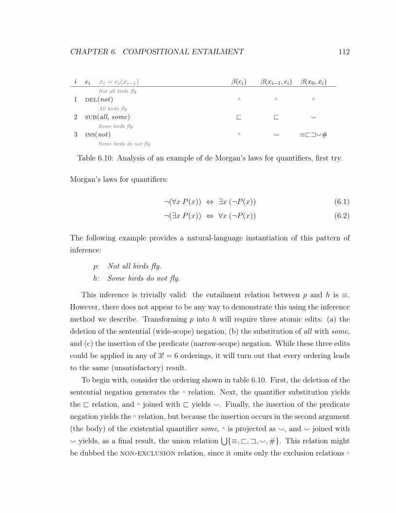
CHAPTER 6. COMPOSITIONAL ENTAILMENT 112
i ei xi = ei(xi−1) β(ei) β(xi−1, ei) β(x0, xi)Not all birds fly
1 del(not) ∧ ∧ ∧
All birds fly
2 sub(all, some) @ @ `Some birds fly
3 ins(not) ∧ ` ≡@A`#Some birds do not fly
Table 6.10: Analysis of an example of de Morgan’s laws for quantifiers, first try.
Morgan’s laws for quantifiers:
¬(∀x P (x)) ⇔ ∃x (¬P (x)) (6.1)
¬(∃x P (x)) ⇔ ∀x (¬P (x)) (6.2)
The following example provides a natural-language instantiation of this pattern ofinference:
p: Not all birds fly.h: Some birds do not fly.
This inference is trivially valid: the entailment relation between p and h is ≡.However, there does not appear to be any way to demonstrate this using the inferencemethod we describe. Transforming p into h will require three atomic edits: (a) thedeletion of the sentential (wide-scope) negation, (b) the substitution of all with some,and (c) the insertion of the predicate (narrow-scope) negation. While these three editscould be applied in any of 3! = 6 orderings, it will turn out that every ordering leadsto the same (unsatisfactory) result.
To begin with, consider the ordering shown in table 6.10. First, the deletion of thesentential negation generates the ∧ relation. Next, the quantifier substitution yieldsthe @ relation, and ∧ joined with @ yields `. Finally, the insertion of the predicatenegation yields the ∧ relation, but because the insertion occurs in the second argument(the body) of the existential quantifier some, ∧ is projected as `, and ` joined with` yields, as a final result, the union relation
⋃{≡,@,A,`,#}. This relation might
be dubbed the non-exclusion relation, since it omits only the exclusion relations ∧

CHAPTER 6. COMPOSITIONAL ENTAILMENT 113
i ei xi = ei(xi−1) β(ei) β(xi−1, ei) β(x0, xi)Not all birds fly
1 del(not) ∧ ∧ ∧
All birds fly
2 ins(not) ∧ | AAll birds do not fly
3 sub(all, some) @ @ ≡@A`#Some birds do not fly
Table 6.11: Analysis of an example of de Morgan’s laws for quantifiers, second try.
and |. Because this result contains the desired result (namely ≡), it is not incorrect,but it is far less informative than we would hope.
Different orderings of the three required edits lead to the same outcome. Forexample, if we insert the predicate negation before we perform the quantifier substi-tution, then we obtain the analysis shown in table 6.11. As before, the deletion of thesentential negation generates the ∧ relation. But this time, the insertion of the pred-icate negation occurs in the second argument (the body) of the universal quantifierall, so that the lexical entailment relation ∧ is projected as | (see section 6.2.4), and ∧
joined with | yields A. Finally, the quantifier substitution generates @, and A joinedwith @ again yields the non-exclusion relation: not incorrect, but under-specific.
While we won’t bother to work through the details here, it can be shown that eachof the six possible orderings of the three required edits leads to the same result, albeitvia different intermediate steps. The problem could perhaps be solved by allowingmore complex edit operations to count as atomic, and by specifying the appropriatelexical entailment relations generated by these richer edits. In our example, it wouldsuffice to treat the quantifier substitution and the insertion of predicate negation asa single atomic edit which generates the ∧ relation. However, such an ad-hoc solutionhas little to recommend it.
6.5.5 A more complex example
Let’s now look at a more complex example that demonstrates the interaction of anumber of aspects of the model we’ve presented. The inference is:

CHAPTER 6. COMPOSITIONAL ENTAILMENT 114
i ei xi = ei(xi−1) β(ei) β(xi−1, ei) β(x0, xi)Jimmy Dean refused to move without blue jeans
1 sub(Jimmy Dean, James Dean) ≡ ≡ ≡James Dean refused to move without blue jeans
2 del(refuse to) | | |James Dean moved without blue jeans
3 ins(did) ≡ ≡ |James Dean did move without blue jeans
4 ins(n’t) ∧ ∧ @James Dean didn’t move without blue jeans
5 sub(move, dance) A @ @James Dean didn’t dance without blue jeans
6 del(blue) @ @ @James Dean didn’t dance without jeans
7 sub(jeans, pants) @ @ @James Dean didn’t dance without pants
Table 6.12: Analysis of a more complex inference, first try.
p: Jimmy Dean refused to move without blue jeans.h: James Dean didn’t dance without pants.
Of course, the example is quite contrived, but it has the advantage that it compactlyexhibits several phenomena of interest: semantic containment (between move anddance, and between pants and jeans); semantic exclusion (in the form of negation);an implicative (namely, refuse to); and nested inversions of monotonicity (created byrefuse to and without).
In this example, the premise p can be transformed into the hypothesis h by asequence of seven edits, as shown in table 6.12. (This time we include even “light”edits, for completeness.) We analyze these edits as follows. The first edit simplysubstitutes one variant of a name for another; since both substituends denote thesame entity, the edit generates the ≡ relation. The second edit deletes an implicative(refuse to) with implication signature –/◦. As described in section 6.3.2, deletions ofthis signature generate the | relation, and ≡ joined with | yields |. The third editinserts an auxiliary verb (did); since auxiliaries are more or less semantically vacuous,this generates the ≡ relation, and | joined with ≡ yields | again. The fourth editinserts a negation, generating the ∧ relation. Here we encounter the first interesting

CHAPTER 6. COMPOSITIONAL ENTAILMENT 115
i ei xi = ei(xi−1) β(ei) β(xi−1, ei) β(x0, xi)Jimmy Dean refused to move without blue jeans
1 ins(did) ≡ ≡ ≡Jimmy Dean did refuse to move without blue jeans
2 ins(n’t) ∧ ∧ ∧
Jimmy Dean didn’t refuse to move without blue jeans
3 del(blue) @ A |Jimmy Dean didn’t refuse to move without jeans
4 sub(jeans, pants) @ A |Jimmy Dean didn’t refuse to move without pants
5 sub(move, dance) A A |Jimmy Dean didn’t refuse to dance without pants
6 del(refuse to) | ` @Jimmy Dean didn’t dance without pants
7 sub(Jimmy Dean, James Dean) ≡ ≡ @James Dean didn’t dance without pants
Table 6.13: Analysis of a more complex inference, second try.
join: as explained in section 5.6, | joined with ∧ yields @. The fifth edit substitutesmove with its hyponym dance, generating the A relation. However, because the editoccurs within the scope of the newly-introduced negation, A is projected as @, and@ joined with @ yields @. The sixth edit deletes a generic modifier (blue), whichgenerates the @ relation by default. This time the edit occurs within the scope of twodownward-monotone operators (without and negation), so we have two inversions ofmonotonocity, and @ is projected as @. Again, @ joined with @ yields @. Finally,the seventh edit substitutes jeans with its hypernym pants, generating the @ relation.Again, the edit occurs within the scope of two downward-monotone operators, so @
is projected as @, and @ joined with @ yields @. Thus p entails h.Of course, the edit sequence shown is not the only sequence which can transform p
into h. A different edit sequence might yield a different sequence of intermediate steps,but the same final result. Consider, for example, the edit sequence shown in table 6.13.Note that the lexical entailment relation β(ei) generated by each edit is the sameas before. But because the edits involving downward-monotone operators (namely,ins(n’t) and del(refused to)) now occur at different points in the edit sequence, manyof the atomic entailment relations β(xi−1, ei) have changed, and thus the sequence of

CHAPTER 6. COMPOSITIONAL ENTAILMENT 116
i ei xi = ei(xi−1) β(ei) β(xi−1, ei) β(x0, xi)Jimmy Dean refused to move without blue jeans
1 ins(did) ≡ ≡ ≡Jimmy Dean did refuse to move without blue jeans
2 ins(not) ∧ | |Jimmy Dean did refuse not to move without blue jeans
3 del(refuse to) | | ≡@A|#Jimmy Dean didn’t move without blue jeans
4 del(blue) @ @ •Jimmy Dean didn’t move without jeans
5 sub(jeans, pants) @ @ •Jimmy Dean didn’t move without pants
6 sub(move, dance) A A •Jimmy Dean didn’t dance without pants
7 sub(Jimmy Dean, James Dean) ≡ ≡ •James Dean didn’t dance without pants
Table 6.14: Analysis of a more complex inference, third try.
joins has changed as well. In particular, edits 3 and 4 occur within the scope of threedownward-monotone operators (negation, refuse, and without), with the consequencethat the @ relation generated by each of these lexical edits is projected as A. Likewise,edit 5 occurs within the scope of two downward-monotone operators (negation andrefuse), and edit 6 occurs within the scope of one downward-monotone operator(negation), so that | is projected as `. Nevertheless, the ultimate result is still @.
However, it turns out not to be the case that every edit sequence which trans-forms p into h will yield equally satisfactory results. Consider the sequence shown intable 6.14. The crucial difference in this edit sequence is that the insertion of not,which generates lexical entailment relation ∧, occurs within the scope of refuse, sothat ∧ is projected as atomic entailment relation | (see section 6.3.4). But the dele-tion of refuse to also produces atomic entailment relation | (see section 6.3.2), and |joined with | yields a relatively uninformative union relation, namely
⋃{≡,@,A, |,#}
(which could also be described as the non-exhaustion relation). The damage hasbeen done: further joining leads directly to the “black hole” relation •, from whichthere is no escape.
Note, however, that even for this infelicitous edit sequence, our inference method

CHAPTER 6. COMPOSITIONAL ENTAILMENT 117
has not produced an incorrect answer (because the • relation includes the @ relation),only an uninformative answer (because it includes all other relations in B as well). Infact, through all the examples we have considered, we have encountered no evidencethat our inference method is unsound, i.e., that it can lead to an incorrect (as opposedto merely uninformative) result. We’ll consider whether this is true in general in thefinal section of this chapter.
6.6 Is the inference method sound?
We have seen that the inference method described in section 6.4 is able to produce thedesired entailment relation (that is, one which is not only correct but as informativeas possible) on a broad variety of example problems, including inferences involv-ing semantic containment, semantic exclusion, implicativity, and nested inversions ofmonotonicity. We have also seen that the method fails to achieve inferential complete-ness : that is, there exist valid inferences (such as instantiations of de Morgan’s lawsfor quantifiers, section 6.5.4) for which the method is not able to produce the desiredentailment relation, but only a less informative (though compatible) relation. Whatabout the converse property of inferential soundness? When the inference methodproduces an informative result, can we be confident that the result is correct?
Unfortunately, we cannot provide a formal proof of soundness. Indeed, to seeksuch a proof would be to misconstrue the very purpose of natural logic, which is, at itsheart, a model of informal reasoning. It is true, of course, that in order to make themodel precise and to implement it in code, we have erected a certain amount of formalscaffolding: the definition of the set B of basic entailment relations and the algebra oftheir joins (chapter 5), and the notion of projectivity signatures (this chapter). Thisformal framework, if divorced from natural language and viewed purely as a calculusof set relations, would no doubt support a formal proof of soundness. But such acalculus would not be a model of natural logic, nor would it provide an account ofnatural language inference; thus, it is a topic for another dissertation.
In a model of natural language inference, the informality of natural languagenecessarily intrudes. The correctness of results produced by the inference method

CHAPTER 6. COMPOSITIONAL ENTAILMENT 118
described in section 6.4 depends on many factors which defy formalization. First, asnoted above, we must find a suitable sequence of edits which transforms p into h (andthe inference method per se offers no guidance on how to find such a sequence, orindeed, whether one exists). Second, we must predict the correct entailment relationfor each edit. Cases like sub(jeans, pants) are straightforward enough, but (as wenoted in section 6.1) other cases are not so clear-cut. Lexical ambiguity is one issue:whether bank @ building depends on which sense of bank is intended. Vagueness isanother: does three @ several? Does method ≡ strategy? Finally, we must correctlydetermine the projectivity properties of semantic functions in our sentences, andproperly identify the extent of their arguments. Classic scope ambiguities (as in Everyman loves some woman) may be one issue, but there are other potential sources ofdifficulty. For example, we noted in section 6.2.5 that while most verbs project | as#, those which encode functional relations project | as |. But whether a particularverb encodes a functional relation may not be entirely clear-cut.
Many of the difficulties just described involve properly identifying the seman-tic properties of lexical items involved in the inference. A further consideration—though it is purely theoretical—is that lexical items exhibiting certain combinationsof semantic properties could, in principle, render our inference method unequivocallyunsound.8 Suppose there were an English adverb X-ly having the following (admit-tedly bizarre) combination of properties: first, it is semantically vacuous (so thatβ(del(X-ly)) = ≡); and second, it is downward monotone (so that its projectivitysignature includes {@:A}). Now consider the following inference:
p: John runs X-ly.h: John moves.
Here, p is transformed into h by two edits, which can occur in either order:sub(runs, moves) and del(X-ly). Of course, β(sub(runs, moves)) = @. Now, theresult produced by the inference method will depend upon the order in which theedits are applied. If we first apply the del and then the sub, the result is @, becausethe del is semantically vacuous, and after it has occurred, X-ly is no longer present
8The following example is due to an anonymous reviewer for the Eighth International Conferenceon Computational Semantics, to whom we are indebted.

CHAPTER 6. COMPOSITIONAL ENTAILMENT 119
to affect the sub, which generates @. However, if we first apply the sub and thenthe del, then the result is A, because the presence of the downward-monotone X-lycauses the lexical entailment relation @ produced by the sub to be projected as A.Since it is not possible that p @ h and p A h, at least one of these two results mustbe incorrect. Therefore, if expressions like X-ly can occur in natural language, thenat least some edit orders can cause our inference method to produce incorrect results.
We are not aware of any actual natural language expression having the unusualcombination of properties exemplified by X-ly. Indeed, it is difficult to imagine thatsuch an expression could be coined—what, exactly, might it mean? It therefore seemsa plausible hypothesis that expressions like X-ly do not occur in natural languages,and consequently that, in practice if not in principle, such expressions pose no threatto the soundness of our inference method. This claim resembles the typological claimsthat have been made about certain monotonicity patterns of quantifiers existing innatural languages. But because we can offer no concrete evidence to support thisclaim, it remains a hypothesis only.
Whatever the theoretical limitations of our model of natural logic, it has beenshown in practice successfully to address a wide range of inference problems. Insection 6.5, we illustrated this using a variety of toy examples; in chapter 7, we willdescribe a computational implementation of this model and a large-scale evaluationof its effectiveness on real-world inference problems.

Chapter 7
The NatLog system
The model of natural logic developed in chapters 5 and 6 may be an elegant theory,and we have seen that it successfully explains a handful of contrived examples. Butis the model just a toy, or can it be effectively implemented and applied to real-world examples of natural language inference? This chapter aims to answer thosequestions.1
The NatLog system is a Java implementation of our model of natural logic. In thefollowing pages, we present the high-level architecture of the system (section 7.1) andprovide detailed descriptions of each of its five key components (sections 7.2 through7.6). Next, we illustrate the operation of the system (section 7.7) using a concreteexample first introduced in the previous chapter. We then discuss evaluations ofthe effectiveness of the system on two well-known collections of NLI problems: theFraCaS test suite (section 7.8) and the RTE3 test suite (section 7.9).
7.1 System architecture
The NatLog system uses a multi-stage pipelined architecture in which the task ofalignment (that is, identifying corresponding entities and predicates in p and h) isdistinguished from the task of entailment classification (determining whether p entailsh). While this division of labor may seem obvious, it is by no means a given: in many
1The material in this chapter is derived in large part from (MacCartney and Manning 2008).
120

CHAPTER 7. THE NATLOG SYSTEM 121
RTE systems, alignment is not explicitly formulated as a separate task, but is achievedimplicitly as part of entailment classification. In adopting a pipelined approach, wefollow a precedent established by Marsi and Krahmer (2005), and developed further inthe Stanford RTE system, as described in (MacCartney et al. 2006) and in chapter 4of this dissertation.
As we saw in chapter 4, the Stanford RTE system uses a pipeline of three stages,comprising linguistic analysis, alignment, and entailment classification. The NatLogpipeline has a similar structure, but places far great emphasis on entailment classi-fication, which it divides into three separate stages. Altogether, then, the NatLogpipeline includes five stages of processing:
1. Linguistic analysis (section 7.2) involves applying standard linguistic analysistools (tokenization, lemmatization, parsing, etc.) to the input sentences p and hin order to generate a variety of linguistic annotations which prepare the groundfor further processing.
2. Alignment (section 7.3) means establishing a sequence of atomic edits whichtransforms p into h. The NatLog system does not itself have the capacityto perform alignment, but relies instead on alignments derived from outsidesources (such as the MANLI system introduced in chapter 3, or the StanfordRTE aligner described in chapter 4).
3. Lexical entailment classification (section 7.4) is the core of the NatLogsystem: it uses machine learning and a variety of lexical resources to predict anentailment relation for each atomic edit, based solely on features of the lexicalitems involved, independent of context.
4. Entailment projection (section 7.5) aims to predict the entailment relationwhich holds across each atomic edit by considering the impact of the context inwhich the edit occurs on the lexical entailment relation produced in the previousstage.
5. Entailment joining (section 7.6) combines the atomic entailment relations

CHAPTER 7. THE NATLOG SYSTEM 122
predicted by the preceding stage across the chain of edits in order to producethe entailment relation which holds between p and h.
The following sections describe each of these stages in greater detail.
7.2 Linguistic analysis
The NatLog pipeline begins by applying a number of off-the-shelf linguistic analy-sis tools to the input sentences p and h, in order to generate linguistic annotationswhich will be useful later in processing. We rely on the Stanford parser (Klein andManning 2003), a Penn Treebank-trained statistical parser, for tokenization, part-of-speech tagging, and syntactic phrase-structure parsing. We also generate a lemmafor each word token using a Java port of the finite-state analyzer of Minnen et al.(2001). Lemmas and part-of-speech tags are used in lexical entailment classification(section 7.4), while the syntactic parses are used in entailment projection (section 7.5).However, relative to some other NLI systems, the linguistic pre-processing performedby NatLog is relatively light. In particular, we make no attempt to perform namedentity recognition, coreference resolution, dependency parsing, or semantic role label-ing. While all these kinds of information could potentially be useful in later stagesof processing, we have chosen to focus our development efforts on our core model ofnatural logic, rather than on incremental improvements to linguistic annotation.
This stage includes one other important type of linguistic analysis: monotonicitymarking of p and h, in which we compute the effective monotonicity for each tokenspan in each input sentence. While this computation is actually performed as partof the linguistic analysis stage, logically it forms part of the fourth processing stage(entailment projection); thus we postpone further discussion until section 7.5.
7.3 Alignment
In the second stage of processing, we establish an alignment between the premise pand hypothesis h, represented by a sequence of atomic edits, operating over phrases,

CHAPTER 7. THE NATLOG SYSTEM 123
which transforms p into h. (Following the usage common in the machine translationliterature, we use the term “phrase” to refer to a contiguous span of word tokens,whether or not the tokens constitute a syntactic phrase.) This alignment representa-tion is symmetric and many-to-many, and is general enough to include various otheralignment representations as special cases. We define four edit types:
• an eq edit connects a phrase in p with an equal (by word lemmas) phrase in h• a sub edit connects a phrase in p with an unequal phrase in h• a del edit covers an unaligned phrase in p• an ins edit covers an unaligned phrase in h
Each edit is parameterized by the token indices at which it operates, and edit indicesmay “cross”, permitting representation of movement. (This is the same representationof alignment used by the MANLI system, described in chapter 3.)
The NatLog system does not itself include any facility for finding good alignments;rather, its purview is the identification of entailment relations between aligned sen-tence pairs. NatLog therefore relies on alignments derived from other sources: eitherhuman annotators, or automatic alignment systems such as the MANLI system (chap-ter 3) or the Stanford RTE aligner (chapter 4).
Although NatLog does not itself generate alignments, but merely reads them infrom an outside source, it does perform one important bit of processing as part ofthe alignment stage: name, heuristic ordering of edits. The outside sources fromwhich NatLog obtains alignments typically do not specify any particular ordering inwhich the edits contained in an alignment should be applied. However, the inferencemethod implemented by NatLog requires that such an ordering be established (seesection 6.4), since this ordering defines a path from p to h through intermediate forms,and thereby decomposes the inference problem into a sequence of atomic inferenceproblems, one for each atomic edit. Since NatLog is free to choose whatever editorder it prefers, it uses heuristic rules to select an order which maximizes the benefitof the monotonicity marking performed in the first stage of processing (but describedin section 7.5).

CHAPTER 7. THE NATLOG SYSTEM 124
In particular, NatLog prefers to put del edits at the beginning of the edit se-quence, sub edits in the middle, and ins edits at the end. There is one complication:the relative ordering of edits involving downward-monotone (or non-monotone) op-erators (e.g., the deletion of not) may influence the effective monotonicity applicablefor other edits. Therefore, in choosing an edit order, NatLog places any edits involv-ing downward-monotone (or non-monotone) operators in a separate group, after allother del and sub edits, and before all other ins edits. This has the benefit thatwhen NatLog needs to compute the effective monotonicity for a particular edit (inthe fourth stage), it is able to use the monotonicity markings on p for all ordinarydel and sub edits, and the monotonicity markings on h for all ordinary ins edits.(By “ordinary”, we simply mean “not involving downward-monotone or non-monotoneoperators”.)
7.4 Predicting lexical entailment relations
Much of the heavy lifting in the NatLog system is done in the third stage of pro-cessing, by the lexical entailment model, which is a concrete implementation of theprinciples described in section 6.1. This model has the job of predicting a lexicalentailment relation for each atomic edit in the alignment determined in the previousstage. Its prediction is based solely on features of the lexical items involved in the edit,independent of the projective properties of the context in which the edit occurs. (Forexample, this model should assign the entailment relation A to the edit sub(weapon,rifle), regardless of whether the context at the locus of the edit is upward-monotone,downward-monotone, or something else.)
To makes its predictions, the lexical entailment model uses machine learning tech-niques, and exploits a plethora of external lexical resources containing informationabout relationships between word meanings. For each edit, the model generates a fea-ture representation (section 7.4.1) which encapsulates all available information aboutthe type of the edit and the words involved in the edit, and then applies a decision treeclassifier (section 7.4.2) which has been trained on a large set of manually-annotatedlexical entailment problems.

CHAPTER 7. THE NATLOG SYSTEM 125
7.4.1 Feature representation
The process of predicting a lexical entailment relation for a given atomic edit beginswith generating a feature representation of the edit, which is a real-valued vectorencoding a variety of information about the edit: its type, its size, characteristicsof the words involved the edit, and (in the case of sub edits) information aboutthe semantic relationship between the substituends. This feature representation thenserves as an input to the classifier described in section 7.4.2.
We begin by describing the features active for sub edits, in which we are particu-larly concerned with the semantic relationship between the substituends, that is, thephrases (often single words) from p and h involved in the edit.
WordNet-derived features. Perhaps the most important features for sub editsare those which exploit WordNet to measure the semantic relatedness of the sub-stituends, using various relation types, including synonymy, antonymy, and hyper-nymy. Each of these features takes values on the interval [0..1].
• The WNSyn feature indicates synonymy: it takes value 1 iff the substituends aresynonyms per WordNet (i.e., belong to the same synset), and 0 otherwise.
• The WNAnt feature indicates antonymy: it takes value 1 iff the substituends areantonyms per WordNet, and 0 otherwise.
• The WNHyper feature indicates hypernymy. If the h phrase is a (direct or in-direct) hypernym of the p phrase in WordNet, then WNHyper takes the value1 − n
8, where n if the number of links which must be traversed in the Word-
Net hypernym hierarchy to get from the p phrase to the h phrase. Other-wise, WNHyper takes value 0. For example, WNHyper(owl , bird) = 0.75, whileWNHyper(bird , owl) = 0.0.
• The WNHypo feature indicates hyponymy, and is simply the inverse of the WNHyperfeature. Thus WNHypo(owl , bird) = 0.0, while WNHypo(bird , owl) = 0.75.

CHAPTER 7. THE NATLOG SYSTEM 126
• The JiCo feature is a measure of semantic relatedness based on the well-knownJiang-Conrath WordNet distance metric (Jiang and Conrath 1997), which mea-sures the distance between two WordNet synsets s1 and s2 as
dJC(s1, s2)def= IC(s1) + IC(s2)− 2 · IC(lso(s1, s2))
where IC(s) is the information content of synset s (that is, the negative of thelogarithm of its frequency of occurrence in a large corpus), and lso(s1, s2) isthe least superordinate (most specific hypernym) of synsets s1 and s2. Possiblevalues for dJC range from a minimum of 0 (for synonyms) to a theoreticalmaximum of 2 · maxs(IC(s)). Thus, to convert dJC to a measure of semanticrelatedness on [0..1], we use
JiCo(s1, s2)def= 1− dJC(s1, s2)
2 ·maxs(IC(s))
This formula gives results that are intuitively pleasing, although it has theconsequence that comparatively few pairs of terms receive a score near 0.
Features based on other lexical resources. In addition to the WordNet-basedfeatures, we use a few other features based on external lexical resources which arein some ways complementary to WordNet. Like the WordNet-based features, thesefeatures have values on [0..1].
• The NomB feature uses information from the NomBank lexical resource (Mey-ers et al. 2004) to indicate derivationally related words having different partsof speech, particularly nominalizations. We extracted from the NOMLEX-PLUS.0.8 file about 4,000 related noun/verb pairs (such as accusation/accuse)and about 2,500 related adjective/adverb pairs (such as angry/angrily). TheNomB feature is set to 0.75 if the substituends are among these pairs, or to 0otherwise.
• The DLin feature is a measure of semantic relatedness based on a thesauruscompiled automatically by Dekang Lin (Lin 1998). This resource, which covers

CHAPTER 7. THE NATLOG SYSTEM 127
nouns, verbs, and adjectives, estimates the relatedness between a pair of wordsor phrases by measuring their distributional similarity, that is, the similarity be-tween the distributions, in a very large corpus, of the grammatical relationshipsin which they participate. It is thus a useful complement to the information ob-tained from manually-compiled resources like WordNet and NomBank. Becausethe scores obtained from the thesaurus are not normalized, we map them onto[0..1] by dividing every score by the maximum score observed in the thesaurus(separately for each part of speech).
String similarity features. Since no static lexical resource can possibly containevery pair of words which might be encountered, the robustness of the system canbe greatly enhanced by including features which measure only string similarity. Suchfeatures are particularly helpful for identifying the equivalence between different ver-sions of proper names, which are commonly missing from static lexical resources. Forexample, string similarity can help us to identify alternate or erroneous spellings of aname (Ahmadinejad, Ahmadi-Nejad, or Ahmadinejab), or shorter and longer versionsof the same name (Lincoln vs. Abraham Lincoln).
• The LemStrSim feature estimates the similarity between words w1 and w2 usinga function based on the string edit distance between the word lemmas:
LemStrSim(w1, w2) = max
[0, 1− dist(lemma(w1), lemma(w2))
max(|lemma(w1)|, |lemma(w2)|)− k
]Here lemma(w) denotes the lemma of word w, as generated by the finite statetransducer of Minnen et al. (2001); dist() denotes Levenshtein string edit dis-tance (Levenshtein 1966); and |·| denotes string length. k is a penalty parameterwhose purpose is to prevent assigning high similarity to very short pairs of un-related words with similar spelling, such as or and for, or she and the. Forexample, if k = 0, then LemStrSim(she, the) = 0.67, but if k = 2 (the valued weused in practice), then LemStrSim(she, the) = 0.0. The similarity assigned tolonger word pairs is less affected by the penalty parameter. For example, withk = 2, LemStrSim(Ahmadinejad ,Ahmadinejab) = 0.89.

CHAPTER 7. THE NATLOG SYSTEM 128
• The LemSubSeq feature is designed to identify the case where one of the sub-stituends is a multi-word phrase which contains the other as a sub-phrase, as insub(Lincoln, Abraham Lincoln) or sub(Dick and Jane, Jane). Unlike the otherfeatures presented so far, the LemSubSeq feature takes values which are entail-ment relations (and which are subsequently encoded by a bundle of booleanfeatures). In particular:
– LemSubSeq(p, h) = @ iff h is a subsequence of p– LemSubSeq(p, h) = A iff p is a subsequence of h– LemSubSeq(p, h) = ≡ iff p and h are equal– LemSubSeq(p, h) = # otherwise
As the name suggests, the LemSubSeq feature works by comparing word lemmas,not merely surface forms.
Lexical category features. We also include a number of features which describethe lexical categories to which the substituends belong.
• The Light feature is a boolean feature which is activated just in case bothsubstituends contain only semantically “light” words, that is, words which havea limited impact on the semantics of the sentences in which they appear. Theintent is that substitutions involving light words should be predicted to gener-ate lexical entailment relation ≡. We define light words to include punctuation,prepositions, possessive markers, articles, auxiliary verbs, and expletives. Ofcourse, we do not mean to make a strong claim that all such words are seman-tically vacuous—rather, this definition reflects a pragmatic choice which seemsto work well in practice.
• The Preps feature is a boolean feature which is activated just in case bothsubstituends are prepositions. The presence of this feature encourages NatLogto be somewhat liberal (i.e., biased toward predicting ≡) regarding substitutionsinvolving prepositions. As we argued in section 6.1.2, this is often—though notalways—an appropriate choice.

CHAPTER 7. THE NATLOG SYSTEM 129
• The Pronoun feature is a boolean feature which is activated just in case bothsubstituends are pronouns. The presence of this feature encourages NatLog tobe somewhat liberal regarding substitutions involving pronouns.
• The NNNN feature is a boolean feature which is activated just in case eitherboth substituends are common nouns, or both substituends are proper nouns.The motivation for this feature is to encode the background assumption thatmost such pairs of nouns should (in the absence of evidence to the contrary) bepredicted to stand in the | relation, as described in section section 6.1.1. Forexample, we want apple | banana and Atlanta | Boston. Of course, for specificpairs of nouns, the ≡, @, or A relation might be more appropriate, but we hopethat in such cases some other featurizer will provide the evidence we need tomake that prediction.
• The Quantifier feature is designed to enable predicting appropriate lexicalentailment relations for sub edits involving quantifier phrases, as outlined insection 6.1.2. Its output space is the set B of basic entailment relations, andits value is intended to serve as the predicted lexical entailment relation forthe given substitution. This feature function contains quite a bit of manuallyencoded knowledge. It defines a number of quantifier categories, such as:
– ALL: including all, every, each, both, everybody, etc.– SOME: including some, something, several, one or more, etc.– NONE: including no, nothing, nobody, no one, neither, etc.– NUM: specific cardinal numbers
In all, we define about a dozen quantifier categories, along with patterns usedto identify occurrences of each category. Finally, for many category pairs, wedefine relations in B which should be predicted to result from a substitution ofquantifiers in those categories. So, for example, we have:
sub(ALL, SOME) → @
sub(ALL, NONE) → |sub(ALL, NUM) → #

CHAPTER 7. THE NATLOG SYSTEM 130
and so on. These definitions are driven both by theory and by pragmatism. Ifeither substituend fails to be recognized as a quantifier phrase, or if we have notdefined a predicted entailment relation for the given pair of quantifier categories,then the feature takes value #.
Miscellaneous additional features for sub edits. Our feature representationincludes a couple of additional features which do not fit neatly into any of the pre-ceding feature categories.
• The NeqNum feature is a boolean feature designed to identify number mis-matches. It is activated just in case the substituends are both numbers andare not equal.
• The MiscSub feature is used to encode knowledge about specific pairs of expres-sions which do not fit neatly into any of the other features. Its output space isthe set B of basic entailment relations, and it includes hand-coded mappingsfrom specific pairs of expressions to lexical entailment relations which should bepredicted for sub edits involving those pairs. In particular, the MiscSub featureencodes the knowledge that:
– sub(and, or) should yield @.– sub edits involving different ways of expressing the genitive (e.g., ’s, of,
his, her, its) should yield ≡.– sub edits involving certain pairs of prepositions should yield | (e.g., after| before, inside | outside), rather than the default ≡.
What about del and ins edits? These are handled as one: in fact, when askedto predict a lexical entailment relation for an ins edit, NatLog first converts it toa del edit (by swapping the roles of p and h), then applies the lexical entailmentmodel (which is designed for del edits), and then returns the converse of the resultingprediction (for example, swapping @ and A).
The feature representation used for del edits is much smaller than the one usedfor sub edits. (As noted in section 6.1.3, most del edits just have @ as the target

CHAPTER 7. THE NATLOG SYSTEM 131
lexical entailment relation, so this is an easier prediction problem.) In fact, for del
edits, we use only the Light and Pronoun features, plus an additional feature whichapplies only to dels:
• The MiscDel feature is used to encode knowledge about specific expressionswhich do not fit neatly into any of the other features. Its output space is theset B of basic entailment relations, and it includes hand-coded mappings fromspecific expressions to lexical entailment relations which should be predicted fordel edits involving those pairs. In particular, the MiscDel feature encodes theknowledge that:
– del(not) and del(false) should yield ∧, while del(true) should yield ≡.– Certain non-intersective adjectives have non-default behavior. del(fake)
and del(former) should yield |, while del(alleged) should yield #.– Deletions of modal verbs often yield #. Thus del(could) and del(should)
should yield |.
Finally, the MiscDel feature is also where we encode knowledge about lexicalentailment relations generated by deletions of implicative and factive operators,as described in section 6.3.2 and section 6.3.3. To do this, we use a custom-builtresource which maps a few dozen common implicative and factive operators totheir implication signatures (see section 6.3.1), based on a list obtained fromresearchers at PARC. For example, this map tells us that force has implicationsignature +/◦, and thus del(force) should yield @; while fail has implicationsignature −/+, and thus del(fail) should yield ∧.
7.4.2 Classifier training
The feature representation described in section 7.4.1 serves as input to a classifierwhose job is to predict lexical entailment relations. For this purpose, we use a J48decision tree classifier from the Weka machine learning library (Witten and Frank2005). Our motivation for choosing a decision tree classifier—as opposed to a linearmodel such as a maximum entropy classifier or a support vector machine—is that weexpect the decision space to be richly structured, with most classification decisions

CHAPTER 7. THE NATLOG SYSTEM 132
problems involving sub edits (1,525 examples)reln count examples≡ 1,042 sub(blast, explosion), sub(had, has), sub(Alfred Nobel, Nobel)@ 95 sub(jet, plane), sub(Italy, nation), sub(deafening, loud)A 86 sub(robots, mini-robots), sub(acquired, bought), sub(some, one)∧ 8 sub(no, some), sub(confirmed, unconfirmed)| 191 sub(1972, 1975 ), sub(Rwanda, Uganda), sub(salt, vinegar)` 0# 103 sub(fetal, human), sub(gatherers, pygmies), sub(baby, girl)
problems involving del edits (924 examples)reln count examples≡ 191 del(has), del(manage to), del(genuine)@ 694 del(last week), del(predictably), del(single)A 3 del(tried to)∧ 6 del(not), del(forgot to), del(it is false that)| 7 del(former), del(refused to), del(prevented)` 2 del(hesitate to)# 21 del(may), del(needed to), del(concluded)
Table 7.1: Examples of training problems for the lexical entailment model.
hinging on just one or two features. While linear models excel at combining evidencefrom a large number of features, in our problem setting we anticipate comparativelylittle need to combine evidence.
In order to train the classifier, we constructed a training set containing 2,449 lexicalentailment problems, derived from alignments of NLI problems from various sources.Of these problems, 1,525 represented sub edits, and consisted of a pair of words orphrases. The other 924 represented del edits, and consisted of just a single word orphrase. Each problem was manually annotated with one of the seven relations in B,indicating the lexical entailment relation generated by the given edit. As table 7.1makes clear, the distribution of data was far from even. Because the problems were

CHAPTER 7. THE NATLOG SYSTEM 133
derived from actual alignments, most sub problems consisted of pairs of equal (ornearly equal) expressions, and thus were labeled with relation ≡. The second mostcommon label for sub problems was |; many of these problems contained pairs of un-equal proper nouns or mutually exclusive common nouns. Among the del problems,the overwhelming majority were labeled with relation @, reflecting the prevalence ofintersective modification, as described in section 6.1.3. The second most commonlabel for del problems was ≡; most such problems involved expressions treated assemantically vacuous, such as auxiliary verbs, though a few involved implicatives.
During training, the decision tree was minimally pruned, and the resulting treecontains about 180 leaves. When tested on the training data, the classifier achieves>99% accuracy, indicating that our feature representation successfully captures nearlyall relevant distinctions between examples.
7.5 Entailment projection
Whereas the third stage predicts a lexical entailment relation for each edit, it is thejob of the fourth stage of processing to determine the atomic entailment relationwhich holds across each edit: that is, the entailment relation which holds betweensuccessive intermediate forms in the path from p to h defined by the alignment. Aswe described in section 6.2, this atomic entailment relation will depend not onlyon the lexical entailment relation produced by the edit (which is independent ofcontext), but also on the projective properties of the context in which the edit occurs.Thus, predicting atomic entailment relations involves two tasks: first, establishingthe projective properties which apply in different regions of the sentences involvedin the problem; and second, determining how these properties affect the projectionof lexical entailment relations into atomic entailment relations for specific edits. Wedescribe the first of these tasks as monotonicity marking and the second as predictingprojections.

CHAPTER 7. THE NATLOG SYSTEM 134
unary operator: withoutpattern: IN < /^[Ww]ithout$/argument 1: monotonicity down on dominating PP
pattern: __ > PP=proj
binary operator: mostpattern: JJS < /^[Mm]ost$/ !> QPargument 1: monotonicity non on dominating NP
pattern: __ >+(NP) (NP=proj !> NP)argument 2: monotonicity up on dominating S
pattern: __ >> (S=proj !> S)
Figure 7.1: Some monotonicity operator type definitions.
7.5.1 Monotonicity marking
The goal of monotonicity marking is to identify within the sentences p and h anyoperators which have monotonicity down or non, and to predict the likely extent oftheir arguments.
(In an ideal world, we would identify not only operators having monotonicitydown or non, but operators having any projectivity signature other than the onewhich maps each entailment relation to itself. In that case, we would describe thetask as “projectivity marking”, as opposed to simply “monotonicity marking”. The factthat NatLog does only monotonicity marking, rather than full projectivity marking,is one of the limitations of the current system.)
For example, in the sentence Jimmy Dean refused to move without blue jeans, wewant to recognize that refused is a downward-monotone operator whose argument isthe embedded sentence to move without blue jeans, and that without is a downward-monotone operator whose argument is the noun phrase blue jeans. Similarly, in thesentence The best player doesn’t always win, we want to recognize that best is anon-monotone operator whose argument is the noun player, and that doesn’t is adownward-monotone operator whose argument is the entire sentence.
Our choice of a Treebank-trained parser (driven by the goal of broad coverage)somewhat complicates this effort, because the nesting of constituents in phrase-structure parses does not always correspond to the structure of idealized semantic

CHAPTER 7. THE NATLOG SYSTEM 135
composition trees. Our solution is imperfect, but largely effective. We define a list ofmonotonicity operator types (that is, categories of operators with monotonicity down
or non, such as implicatives like refuse, or prepositions like without), and for eachsuch operator type we specify its arity and a Tregex tree pattern (Levy and Andrew2006) which permits us to identify its occurrences in our Treebank parses. We alsospecify, for each argument position of each operator type, both the monotonicity class(down or non) and another Tregex pattern which helps us to determine the likelyextent of the argument in a phrase-structure tree. (Figure 7.1 shows some exampledefinitions.)
Although we have presented monotonicity marking as belonging (logically) tothe fourth stage of NatLog processing, in fact it happens during the first stage, aspart of linguistic analysis. After parsing, we match the tree patterns in each of themonotonicity operator type definitions against the phrase-structure parse trees for pand h, and add annotations to parse tree nodes to indicate constituents which areeither monotonicity operators or arguments thereto.
Note that we make no attempt to resolve scope ambiguities, such as that exhibitedby the sentence Every man loves some woman, but we find that in practice this rarelycauses problems: the default behavior usually leads to the right predictions. Thereare at least three reasons for this. First, inferences which hinge on scope ambiguitiesare rare. Second, the assumption that the first quantifier takes wide scope turns outto be a fairly reliable heuristic. Third, in many cases the effective monotonicity ateach point in the sentence will be same no matter how the scope ambiguity is resolved.This is the case with Every man loves some woman: whether some is interpreted ashaving wide or narrow scope, the effective monotonicity at man will be down, whilethe effective monotonicity in the rest of the sentence will be up.
7.5.2 Predicting projections
Having computed a lexical entailment relation for each edit in the third stage ofprocessing, NatLog uses the monotonicity markings on the parses of p and h to de-termine the projection of each lexical entailment relation into an atomic entailment

CHAPTER 7. THE NATLOG SYSTEM 136
relation. As we described in section 7.3, NatLog facilitates this process by choosingan edit ordering in which del and sub edits not involving monotonicity operatorsare applied first, and ins edits not involving monotonicity operators are applied last.Consequently, in computing the atomic entailment relation for a particular edit, weuse monotonicity markings from p for del and sub edits, and monotonicity markingsfrom h for ins edits. (This strategy can go wrong if there are multiple edits involvingmonotonicity operators, but this rarely occurs in practice. A more principled ap-proach would be separately to compute monotonicity markings on every intermediateform on the path from p to h defined by the alignment.)
Given a parsed sentence with monotonicity markings, how do we actually deter-mine the projection of a given entailment relation? Our first task is to establish theeffective monotonicity at the locus of the edit. First, we find the smallest parse con-stituent containing the tokens involved in the edit. Next, we trace a path upwardthrough the parse tree from this constituent to the root, collecting any monotonicitymarkings we find along the way. (We exclude any monotonicity markings which weregenerated by an operator which is itself an argument to the edit.) If any of thesemarkings is non, we conclude that the effective monotonicity is non. Otherwise,we count the number of markings which are down, and if this number is odd, weconclude that the effective monotonicity is down. Otherwise, we conclude that theeffective monotonicity is up.
If the effective monotonicity is non, then we assume that every lexical entailmentrelation is projected as atomic entailment relation #. If the effective monotonicityis down, then we assume that every lexical entailment relation is projected as itsdual under negation (in the sense of section 5.3.1): thus @ is projected as A, andvice-versa. Finally, if the effective monotonicity is up, then we assume that everylexical entailment relation is projected without change.
7.6 Joining entailment relations
In the final stage of processing, the atomic entailment relations predicted for each edit(which result from the projectivity computations in the previous stage) are combined,

CHAPTER 7. THE NATLOG SYSTEM 137
one by one, across the chain of atomic edits, to produce a final, overall predictionfor the inference problem. The combination is performed using the join operation ondefined in section 5.6. This is a deterministic operation, and is simple to compute. (Infact, the 7×7 join table for relations in B is precomputed, so this stage of processinginvolves only lookups.)
As we alluded to in section 5.6.3, the NatLog system has no need to representunions of relations in B which may result from joining two relations in B. Rather,those joins which would result in a union relation are approximated instead by #.Note that if a chain of joins ever reaches #, then it is “stuck” there: no further joiningcan lead to any other result. Consequently, prediction errors earlier in the processingpipeline are likely to cause the final prediction to be #, and this tendency becomesstronger as the number of atomic edits grows. Because # is the least informativerelation in B (permitting neither the truth nor falsity of one of its arguments to beinferred from the truth or falsity of the other), we might say that NatLog has aninnate tendency to be conservative in its predictions, in the sense that when it runsinto problems, it tends to predict neither entailment nor contradiction.
This chaining of entailments across edits can be compared to the method presentedin (Harmeling 2007); however, that approach assigns to each edit merely a probabilityof preserving truth, not an entailment relation.
7.7 An example of NatLog in action
Because our presentation of the five stages of the NatLog system in sections 7.2through 7.6 has perhaps been rather abstract, we now describe a concrete examplewhich illustrates the operation of the NatLog system. For this purpose, we use aninference problem first introduced in section 6.5.5, namely:
p: Jimmy Dean refused to move without blue jeans.h: James Dean didn’t dance without pants.
During the linguistic analysis stage, these sentences are parsed using the Stanfordparser; the results are shown in figure 7.2. The operation of the remaining four stagesis depicted in table 7.2.

CHAPTER 7. THE NATLOG SYSTEM 138
(S(NP (NNP Jimmy) (NNP Dean))(VP (VBD refused)
(S(VP (TO to)
(VP (VB move)(PP (IN without)
(NP (JJ blue) (NNS jeans)))))))(. .))
(S(NP (NNP James) (NNP Dean))(VP (VBD did) (RB n’t)
(VP (VB dance)(PP (IN without)
(NP (NNS pants)))))(. .))
parse for p parse for h
Figure 7.2: Syntactic parses for the p and h sentences of the James Dean example.
lexical atomic cum.edit features entrel mono entrel join
1 del(blue) @ up @ @
2 sub(Jimmy Dean, James Dean) strsim:0.67 ≡ up ≡ @
3 sub(move, dance) hyponym A down @ @
4 eq(without, without) ≡ down ≡ @
5 sub(jeans, pants) hypernym @ up @ @
6 del(refused to) implic:+/◦ | up | |7 ins(n’t) cat:neg ∧ up ∧ @
8 ins(did) cat:aux ≡ down ≡ @
Table 7.2: An example of the operation of the NatLog model.
The best alignment for this example is fairly easy to identify, and the edits itcontains appear as the first column table 7.2. Note, however, that these edits havebeen ordered according to the heuristics described in section 7.3: dels first, thensubs, then edits which involve operators with non-default projectivity, and inss last.
The second column of table 7.2 shows features generated by the lexical entailmentmodel for each edit. For compactness, we display at most one (especially salient) fea-ture per edit. Jimmy Dean and James Dean have comparatively high string similarity.We use WordNet to identify the other two sub edits as hyponym and hypernym sub-stitutions. The miscDeln feature identifies refuse to as an implicative with signature+/◦, and the final ins edits are distinguished by their lexical categories.

CHAPTER 7. THE NATLOG SYSTEM 139
The third column of table 7.2 shows the lexical entailment relation predicted foreach edit. A generic deletion (edit 1) generates the @ relation. A substitution withhigh string similarity (edit 2) leads to the ≡ relation, as do a match (edit 4), andthe insertion of a semantically vacuous auxiliary (edit 8). The hyponym (edit 3)and hypernym (edit 5) substitutions generate A and @, respectively. The implicativedeletion (edit 6) generates |, according to its implication signature, and the insertionof negation (edit 7) generates the ∧ relation.
The fourth column of table 7.2 shows the effective monotonicity at the locus ofeach edit. (We present monotonicity classes, rather than the more general projectivitysignatures, for simplicity and compactness.) The effective monotonicity for edits 1through 6 is computed from the syntactic parse for p, while the effective monotonicityfor edits 7 and 8 is computed from the syntactic parse for h. In p, refuse to is identifiedas a downward-monotone operator whose scope is its sentential complement, andwithout is identified as a downward-monotone operator whose scope is its argumentnoun phrase. Consequently, edits 1 and 5 occur in an upward-monotone context(since they fall within the scope of two downward-monotone operators), while edits3 and 4 occur in a downward-monotone context (since they fall within the scope ofjust one downward-monotone operator), and edit 2 occurs in an upward-monotonecontext (since it doesn’t fall within the scope of any downward-monotone operators).Meanwhile, in h, not is identified as a downward-monotone operator whose scopeis the sentence in which it appears. Consequently, edit 8 occurs in a downward-monotone context (since it falls within the scope of a downward-monotone operator),while edit 7 occurs in an upward-monotone context (since it doesn’t fall within thescope of any downward-monotone operators).
The fifth column of table 7.2 shows how the lexical entailment relations (fromthe third column) are projected into atomic entailment relations, according to theeffective monotonicity shown in the fourth column. The only noteworthy case is edit3, where the lexical entailment relation A is projected into atomic entailment relation@ by a downward-monotone context.
The sixth and final column of table 7.2 shows the cumulative join of the atomicentailment relations in the fifth column. Initially, these are unremarkable: @ joined

CHAPTER 7. THE NATLOG SYSTEM 140
with either ≡ or @ yields @. But at edit 6, we find that @ joined with | yields |, andat edit 7, we find that | joined with ∧ yields @ again. The final entailment relation inthis line, @, is NatLog’s final (and correct) answer for our example problem.
7.8 Evaluation on the FraCaS test suite
The FraCaS test suite (Cooper et al. 1996) of NLI problems was one product of theFraCaS Consortium, a large collaboration in the mid-1990s aimed at developing arange of resources related to computational semantics. The FraCaS problems containcomparatively simple sentences, and the premise and hypothesis sentences are usu-ally quite similar, so that just a few edits suffice to transform p into h. Despite thissimplicity, the problems are designed to reflect a broad diversity of semantic and infer-ential phenomena. For this reason, the FraCaS test suite has proven to be invaluableas a developmental test bed for the NatLog system and as a yardstick for evaluatingits effectiveness. Indeed, the test suite was created with just such an application asits primary goal. As the authors write:
In light of the view expressed elsewhere in this and other FraCaS de-liverables ... that inferential ability is not only a central manifestation ofsemantic competence but is in fact centrally constitutive of it, it shouldn’tbe a surprise that we regard inferencing tasks as the best way of testingan NLP system’s semantic capacity.2
Despite having been designed expressly for the purpose of evaluating NLI systems,the FraCaS test suite went largely unexploited for more than a decade. In fact, toour knowledge, we are the first to have undertaken a quantitative system evaluationusing the complete FraCaS data set.3
2Cooper et al. (1996), p. 63.3Sukkarieh (2003) uses a handful of FraCaS examples in a manual evaluation of her McLogic for-
malism for knowledge representation and inference, but does not undertake a complete, quantitative,or automatic evaluation.

CHAPTER 7. THE NATLOG SYSTEM 141
7.8.1 Characteristics of the FraCaS test suite
The FraCaS test suite contains 346 NLI problems, each consisting of one or morepremise sentences, (usually) followed by a question and an answer. Figures 1.1 and1.2 show a representative selection of FraCaS problems.
Questions and hypotheses. While the original FraCaS test suite expresses the“goal” of each problem as a question, the standard formulation of the NLI task involvesdetermining the entailment relation between a premise and a declarative hypothesis.Thus, for the purpose of this work, we converted each FraCaS question into a declara-tive hypothesis, using an automatic tool which first generates a syntactic parse of thequestion and then applies a few simple tree-transformation rules. The results werethen manually reviewed for grammaticality. Very few corrections were needed, mostlyinvolving replacing negative-polarity items such as any. (For example, the questionDid any accountant attend the meeting? was automatically transformed into the hy-pothesis Any accountant attended the meeting. Any was then manually changed toSome.)
Answer types. Most FraCaS problems are labeled with one of three answers: yes,no, or unk.4 This three-way formulation of the NLI task was introduced in sec-tion 5.2.2, where we identified the yes label with the entailment relation, the no
label with the contradiction relation, and the unk label with the compatibil-
ity relation. We can also identify each of these three labels with a union of relationsin B, as described in section 5.6.3: yes corresponds to
⋃{≡,@}, no corresponds
to⋃{∧, |}, and unk corresponds to
⋃{A,`,#}. The distribution of answers is not
balanced: about 59% of the problems have answer yes, while 28% have answer unk,4Actually, the answers are not completely standardized, and quite a few contain qualifiers, such
as, “Yes, on one possible reading”. However, in most cases, the given answer can be straightforwardlyidentified with one of the values yes, no, or unk. But 12 of the 346 problems (about 3%) do not fitneatly into this scheme. Four problems lack questions and answers altogether, and in the remainingeight problems, the answer is too ambiguous or complex to be clearly identified with one of thethree labels. Examples of such answers include “Yes on one scoping; unknown on another scoping”,“Not many”, and “At most two”. These 12 problems were omitted from the evaluation described insection 7.8.2.

CHAPTER 7. THE NATLOG SYSTEM 142
and 10% have answer no. Consequently, a most-common-class classifier can achieverespectable accuracy simply by guessing yes on every problem.
Multiple-premise problems. Of the 346 FraCaS problems, 154 (about 45%) con-tain multiple premises: 122 problems contain two premises, 29 problems contain threepremises, two problems contain four premises, and one problem contains five premises.These multiple-premise problems were excluded from the evaluation described in sec-tion 7.8.2. As we noted in section 6.4, an important limitation of the inference methodimplemented by NatLog is that, unlike first-order logic, it provides no general mech-anism for combining information from multiple premises. However, this limitation isnot unique to NatLog: it is faced by all other NLI systems of which we are aware. Tobe sure, most NLI systems—including NatLog—can accept a premise which containsmultiple sentences. Indeed, recent RTE data sets have included an ever-greater pro-portion of problems with multi-sentence premises. But, for the most part, solving suchproblems requires nothing more than extracting information from a single sentence.By contrast, the inference problems shown in figure 1.2 cannot be solved withoutcombining information from multiple sentences. Because NatLog relies on analyzingentailment relations across a single chain of atomic edits, it cannot effectively handlesuch problems. But nor can other systems developed for the RTE challenge.
Sections. The FraCaS test suite is divided into nine sections, each focused on aspecific category of semantic phenomena: (1) quantifiers, (2) plurals, (3) anaphora,(4) ellipsis, (5) adjectives, (6) comparatives, (7) temporal reference, (8) verbs, and(9) attitudes. Of course, some of these sections will be more amenable than others tothe natural logic approach: we hope to do well with quantifiers, but expect to makelittle headway with ellipsis, anaphora, or temporal reference.
7.8.2 Experiments and results
We evaluated the NatLog system on a subset of the FraCaS data containing 183single-premise inference problems (representing about 53% of the complete FraCaSdata set). The test set excluded multiple-premise problems (for reasons discussed in

CHAPTER 7. THE NATLOG SYSTEM 143
System P % R % Acc %baseline: most common class 55.7 100.0 55.7bag of words 59.7 87.2 57.4NatLog 2007 68.9 60.8 59.6NatLog 2008 89.3 65.7 70.5
Table 7.3: Performance of various systems on 183 single-premise FraCaS problems(three-way classification). The columns show precision and recall for the yes class,and accuracy.
section 7.8.1) and a handful of other problems which lack a well-defined answer (seefootnote 4).
The NatLog system depends on alignments (that is, edit sequences connectingp and h) from an outside source. For these experiments, we generated alignmentsautomatically using a very simple dynamic programming algorithm similar to theLevenshtein string edit distance algorithm (Levenshtein 1966), applied at the tokenlevel. The results from this automatic alignment were then manually reviewed andcorrected.
Table 7.3 shows the results of the evaluation, along with some comparisons. Asa baseline, we show results for a most-common-class classifier, which achieves perfectrecall for the yes class (because it always guesses yes), but mediocre precision andaccuracy (equal to the proportion of yes answers in the test set). A slightly strongercomparison is provided by a bag-of-words model like the one described in chapter 2.Relative to the most-common-class classifier, this model achieves lower recall, butslightly better precision and accuracy. Table 7.3 also shows results from an evaluationof an earlier version of the NatLog system, reported in (MacCartney and Manning2007).
The current (2008) version of the NatLog system achieves overall accuracy of over70%, representing a 27% reduction in error from the 2007 version and a 33% reductionin error from the baseline. A particularly noteworthy and gratifying result is the highfigure for precision: over 89% for the current system. Errors in which NatLog wronglypredicts yes have fallen 66% from the 2007 version and 76% from the baseline.
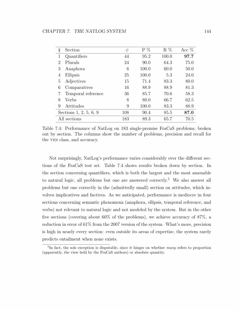
CHAPTER 7. THE NATLOG SYSTEM 144
§ Section # P % R % Acc %1 Quantifiers 44 95.2 100.0 97.72 Plurals 24 90.0 64.3 75.03 Anaphora 6 100.0 60.0 50.04 Ellipsis 25 100.0 5.3 24.05 Adjectives 15 71.4 83.3 80.06 Comparatives 16 88.9 88.9 81.37 Temporal reference 36 85.7 70.6 58.38 Verbs 8 80.0 66.7 62.59 Attitudes 9 100.0 83.3 88.9Sections 1, 2, 5, 6, 9 108 90.4 85.5 87.0All sections 183 89.3 65.7 70.5
Table 7.4: Performance of NatLog on 183 single-premise FraCaS problems, brokenout by section. The columns show the number of problems, precision and recall forthe yes class, and accuracy.
Not surprisingly, NatLog’s performance varies considerably over the different sec-tions of the FraCaS test set. Table 7.4 shows results broken down by section. Inthe section concerning quantifiers, which is both the largest and the most amenableto natural logic, all problems but one are answered correctly.5 We also answer allproblems but one correctly in the (admittedly small) section on attitudes, which in-volves implicatives and factives. As we anticipated, performance is mediocre in foursections concerning semantic phenomena (anaphora, ellipsis, temporal reference, andverbs) not relevant to natural logic and not modeled by the system. But in the otherfive sections (covering about 60% of the problems), we achieve accuracy of 87%, areduction in error of 61% from the 2007 version of the system. What’s more, precisionis high in nearly every section: even outside its areas of expertise, the system rarelypredicts entailment when none exists.
5In fact, the sole exception is disputable, since it hinges on whether many refers to proportion(apparently, the view held by the FraCaS authors) or absolute quantity.
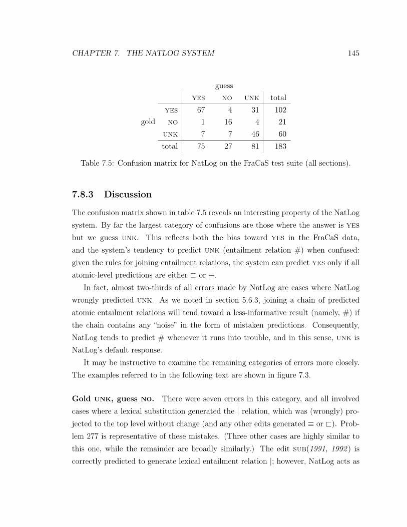
CHAPTER 7. THE NATLOG SYSTEM 145
guess
gold
yes no unk totalyes 67 4 31 102no 1 16 4 21
unk 7 7 46 60total 75 27 81 183
Table 7.5: Confusion matrix for NatLog on the FraCaS test suite (all sections).
7.8.3 Discussion
The confusion matrix shown in table 7.5 reveals an interesting property of the NatLogsystem. By far the largest category of confusions are those where the answer is yes
but we guess unk. This reflects both the bias toward yes in the FraCaS data,and the system’s tendency to predict unk (entailment relation #) when confused:given the rules for joining entailment relations, the system can predict yes only if allatomic-level predictions are either @ or ≡.
In fact, almost two-thirds of all errors made by NatLog are cases where NatLogwrongly predicted unk. As we noted in section 5.6.3, joining a chain of predictedatomic entailment relations will tend toward a less-informative result (namely, #) ifthe chain contains any “noise” in the form of mistaken predictions. Consequently,NatLog tends to predict # whenever it runs into trouble, and in this sense, unk isNatLog’s default response.
It may be instructive to examine the remaining categories of errors more closely.The examples referred to in the following text are shown in figure 7.3.
Gold unk, guess no. There were seven errors in this category, and all involvedcases where a lexical substitution generated the | relation, which was (wrongly) pro-jected to the top level without change (and any other edits generated ≡ or @). Prob-lem 277 is representative of these mistakes. (Three other cases are highly similar tothis one, while the remainder are broadly similarly.) The edit sub(1991, 1992 ) iscorrectly predicted to generate lexical entailment relation |; however, NatLog acts as

CHAPTER 7. THE NATLOG SYSTEM 146
§1: Quantifiers
56 p Many British delegates obtained interesting results from the survey.h Many delegates obtained interesting results from the survey. unk
§2: Plurals
109 p Just one accountant attended the meeting.h Some accountants attended the meeting. no
§4: Ellipsis
176 p John said Mary wrote a report, and Bill did too.h John said Bill wrote a report. yes
§5: Adjectives
217 p John is a cleverer politician than Bill.h John is cleverer than Bill. unk
§7: Temporal reference
277 p Smith lived in Birmingham in 1991.h Smith lived in Birmingham in 1992. unk
304 p Smith wrote a report for two hours.h Smith wrote a report. unk
Figure 7.3: Examples of errors made by NatLog on the FraCaS test suite.

CHAPTER 7. THE NATLOG SYSTEM 147
if the verb lived projects | (from a temporal modifier) without change, when in factit should project | as #. Note the discrepancy between implementation and theory:in section 6.2.5, we noted explicitly that most verbs project | as #. True, we alsoobserved there that verbal constructions which encode functional relations, such aswas born in, do project | as |; however, lived is not such a verb. This type of errorcould be corrected without much difficulty.
Gold unk, guess yes. Each of the seven errors in this category involved a deletionedit for which NatLog rightly predicted lexical entailment relation @, but wronglyassumed that this relation would be projected without change to the top level. Thesole error made in the section on quantifiers (problem 56) is disputable, since it hingeson whether the quantifier many refers to proportion (and thus is non-monotone inits first argument—apparently the view held by the FraCaS authors), or to absolutequantity (and thus is upward-monotone in its first argument). In this author’s view,the latter reading is more intuitive, and NatLog’s answer of yes is in fact correct.The remaining errors in this category involved adjectives, comparatives, and temporalreference, and are typified by problems 217 and 304.
Gold yes, guess no. All four errors in this category involve ellipsis, and all aremore-or-less hopeless cases for NatLog. Problem 176 is a typical example. The align-ment used by NatLog in this problem includes the deletion of the second (elliptical)clause in p, and straightforward linear alignment of the first clause in p to h, includingthe edit sub(Mary, Bill). For this edit, NatLog (rightly) predicts the lexical entail-ment relation |, and consequently produces answer no for the problem. While thereis an alignment which could have led NatLog to the correct answer (namely, the onewhich matches each token in h to the equal token in p, and deletes all other tokens inp), it is unreasonable to expect an aligner to produce it, since that alignment appearspreferable only to one who grasps the phenomenon of ellipsis.
Gold no, guess yes. The sole error in this category was problem 109. NatLogpredicts yes because it (rightly) assigns lexical entailment relation @ to the edit

CHAPTER 7. THE NATLOG SYSTEM 148
sub(one, Some), and because it does not model the restrictive semantics of Just.Note that yes would be the correct answer if not for the s on accountants in h; thus,a further reason for NatLog’s mistake is that it systematically (and intentionally)ignores morphology.
Since the NatLog system was developed with FraCaS problems in mind, theseresults do not constitute a proper evaluation on unseen test data. On the other hand,the system does no training on FraCaS data, and has had no opportunity to learnits biases. (Otherwise, accuracy on §4 could not fall so far below the baseline.) Thesystem not only answers most problems correctly, but usually does so for valid reasons,particular within its areas of expertise. All in all, the results fulfill our main goal intesting on FraCaS: to demonstrate the representational and inferential adequacy ofour model of natural logic.
7.9 Evaluation on the RTE test suite
Because the FraCaS data set is comparatively small, and because it has not beenused to evaluate other NLI systems, making comparisons difficult, we chose also toevaluate NatLog using a larger, better known collection of NLI problems from thePASCAL RTE Challenge, which was introduced in section 1.3.2.
7.9.1 Characteristics of the RTE test suite
The RTE test suites differ from the FraCaS test suite in several important and relevantways. (See figure 7.4 for some example problems.) First, the RTE data sets aremuch larger. Second, the goal of RTE is binary classification (as in section 5.2.1),rather than three-way classification. Third, instead of textbook examples of semanticphenomena, RTE problems are more natural-seeming, and the premises are muchlonger than in FraCaS.
Due to the character of RTE problems, we do not expect NatLog to be a goodgeneral-purpose solution to solving all RTE problems. One reason is that most RTEproblems depend on forms of inference, such as paraphrase, temporal reasoning, or

CHAPTER 7. THE NATLOG SYSTEM 149
71 p As leaders gather in Argentina ahead of this weekends regional talks,Hugo Chávez, Venezuela’s populist president is using an energy windfallto win friends and promote his vision of 21st-century socialism.
h Hugo Chávez acts as Venezuela’s president. yes
85 p Mr. Fitzgerald revealed he was one of several top officials who told Mr.Libby in June 2003 that Valerie Plame, wife of the former ambassadorJoseph Wilson, worked for the CIA.
h Joseph Wilson worked for CIA. no
788 p Democrat members of the Ways and Means Committee, where tax billsare written and advanced, do not have strong small business votingrecords.
h Democrat members had strong small business voting records. no
Figure 7.4: Illustrative examples from the RTE3 development set.
relation extraction, which NatLog is not designed to address. Another reason isthat in most RTE problems, the edit distance between p and h is relatively large.More atomic edits means a greater chance that errors made in lexical entailmentclassification or entailment projection will propagate, via entailment joining, to thesystem’s final output. (Given the rules for entailment joining, the system can answeryes to an RTE problem only if all atomic-level predictions are either @ or ≡.) Rather,in applying NatLog to RTE, we hope to make reliable predictions on a subset ofRTE problems, trading recall for precision. If we succeed, then we may be able tohybridize with a broad-coverage RTE system to obtain better results than eithersystem individually—the same strategy that was adopted by Bos and Markert (2006)for their FOL-based system.
7.9.2 Experiments and results
In order to evaluate NatLog’s effectiveness on RTE problems, we used data from theRTE3 test suite. In these experiments, we used alignments generated by the alignmentcomponent of the Stanford RTE system (chapter 4) as input to our entailment model.

CHAPTER 7. THE NATLOG SYSTEM 150
System Data % Yes P % R % Acc %
NatLog dev 22.5 73.9 32.4 59.3test 26.4 70.1 36.1 59.4
Stanford dev 50.3 68.7 67.0 67.3test 50.0 61.8 60.2 60.5
Hybrid, balanced dev 50.0 70.3 68.2 68.8test 50.0 65.5 63.9 64.3
Hybrid, optimized dev 56.0 69.2 75.2 70.0test 54.5 64.5 68.5 64.5
Table 7.6: Performance of various systems on the RTE3 test suite (two-way classi-fication). The columns show the data set used (development or test, 800 problemseach), the proportion of yes predictions, precision and recall for the yes class, andaccuracy.
Recall that in the Stanford system, an alignment is a map from h words to p words.An h word can be aligned to any p word, regardless of position; multiple h words canbe aligned to the same p word; and there is no notion of phrase alignments. Whenwe translate such alignments into the NatLog representation described in section 7.3,each pair of aligned words generates a sub edit (or, if the words are identical, aneq edit). Unaligned p words yield del edits, while unaligned h words yield ins
edits. Where possible, contiguous sequences of word-level edits are then collectedinto equivalent phrase edits. While the result of this translation method cannot beinterpreted as a conventional edit script (there is no well-defined ordering of edits,and multiple edits can operate on the same input phrases), we find that this poses nogreat impediment to subsequent processing by the entailment model.
The first rows of table 7.6 show the performance of NatLog on RTE3 developmentand test sets, as well as the performance of the Stanford RTE system. The overallaccuracy of the NatLog system is not particularly impressive (below 60%), mainlydue to the fact that most RTE problems involve types of inference where naturallogic is of little help. However, relative to the Stanford system, NatLog achieves highprecision on its yes predictions—above 70%—suggesting that combining the NatLog

CHAPTER 7. THE NATLOG SYSTEM 151
and Stanford systems using a hybridization strategy may be effective. For comparison,the FOL-based system of Bos and Markert (2006) attained a similarly high precisionof 76% on RTE2 problems, but was able to make a positive prediction in only about4% of cases. NatLog makes positive predictions far more often—in about 25% ofcases. Thus, NatLog achieves six times the coverage of the Bos & Markert system,with nearly the same precision.
The Stanford system makes yes/no predictions by thresholding a real-valued in-ference score. To construct a hybrid system, we adjust the Stanford inference scoresby +∆ or −∆, depending on whether or not NatLog predicts yes. We choose ∆
by optimizing development set accuracy, while adjusting the threshold to generatebalanced predictions (that is, equal numbers of yes and no predictions). As an ad-ditional experiment, we fix ∆ at this value and then adjust the threshold to optimizedevelopment set accuracy, resulting in an excess of yes predictions. (Since this opti-mization is based solely on development data, its use on test data is fully legitimate.)Results for these two cases are shown in the last rows of table 7.6. The parameterstuned on development data were found to yield good performance on test data. Theoptimized hybrid system attained an absolute accuracy gain of 4% over the Stanfordsystem, corresponding to an extra 32 problems answered correctly. This result isstatistically significant (p < 0.05, McNemar’s test, 2-tailed).
7.9.3 Discussion
The gains attributable to NatLog are exemplified by problem 788 (figure 7.4). NatLogsanctions the deletion of a restrictive modifier and an appositive from the premise,and recognizes that deleting a negation generates a contradiction; thus it correctlyanswers no. On the other hand, there are many RTE problems where NatLog’sprecision works against it. For example, NatLog answers no to problem 71 becauseit cannot account for the insertion of acts as in the hypothesis. Fortunately, both theStanford system and the hybrid system answer this problem correctly.

Chapter 8
Conclusions
In this dissertation, we have explored a range of approaches to the problem of nat-ural language inference (NLI): first, the robust, but imprecise, bag-of-words model(chapter 2), which predicts inferential validity via approximate matching of lexicalcontent; next, the Stanford RTE system (chapter 4), which preserves the approximatematching strategy, but seeks to add a bit more precision; and finally, natural logic(chapters 5 and 6) and the NatLog system (chapter 7), which aims to address thesubset of NLI problems requiring substantially greater semantic precision. We havealso examined the problem of alignment for NLI (chapter 3), which plays a role ineach of these approaches. What have we learned about the problem of NLI, and whatare the most promising directions for future research in this area? This final chapterseeks to address these questions.
8.1 Contributions of the dissertation
This dissertation has examined the problem of natural language inference from anumber of angles, and we hope to have made important contributions in severaldifferent areas.
In chapter 2, we developed a bag-of-words model for NLI and evaluated it onseveral RTE problem sets. While the basic form of the model is not novel, thespecific details of its construction are original. Perhaps our most important finding
152

CHAPTER 8. CONCLUSIONS 153
was the wide variation in the intrinsic difficulty of the various RTE problem sets, asmeasured by the yardstick of this very simple model.
In chapter 3, we undertook the first systematic investigation of the problem ofalignment for NLI. We examined the relation between alignment in NLI and in ma-chine translation (MT), and presented a number of arguments for the unsuitabilityof MT aligners to the NLI alignment task. We made the first comparative evalu-ation of bag-of-words, MT, and NLI aligners on an NLI alignment task. And, weproposed a new model of alignment for NLI—the MANLI system—and showed thatit significantly outperforms rival approaches, by exploiting external lexical resourcesin a supervised learning paradigm, by including contextual features to aid in aligningfunction words, and by allowing multi-word phrases to be aligned as units.
In chapter 4, we introduced the Stanford RTE system, which was among the firstNLI systems to make a clear separation between alignment and entailment determi-nation. This crucial innovation enables the Stanford RTE system to make predictionsof inferential validity which are based, not merely on the degree of alignment, butalso on global features of the aligned 〈p, h〉 pair motivated by semantic theory. TheStanford RTE system is thereby able to attain substantially greater precision thansimple overlap models such as the bag-of-words model presented in chapter 2.
Seeking still greater precision, we then presented the most important contributionof the dissertation: a new model of natural logic which extends the monotonicitycalculus of van Benthem and Sánchez-Valencia to incorporate semantic exclusionand implicativity. We began in chapter 5 by defining an expressive inventory ofentailment relations—the set B of seven basic entailment relations—which includesrepresentations of both semantic containment and semantic exclusion. We showedthat the relations in B are both mutually exclusive and (if vacuous expressions areexcluded) mutually exhaustive, so that every pair of (non-vacuous) expressions canbe assigned to some relation in B. We also described the algebra of joins for relationsin B, and explained how to compute such joins automatically.
In chapter 6, we introduced the concept of projectivity signatures, which gener-alizes the concept of monotonicity classes to cover the exclusion relations. We then

CHAPTER 8. CONCLUSIONS 154
described a general method for determining the entailment relation between two sen-tences p and h, by (1) finding a sequence of atomic edits which transforms p into h;(2) predicting a lexical entailment relation for each edit; (3) propagating the lexicalentailment relation generated by each edit upward through the semantic compositiontree of the sentence to which the edit is applied, according to the projectivity signa-tures of intermediate nodes; and (4) joining the resulting entailment relations acrossthe edit sequence. And, we showed how to provide a unified account of inferencesinvolving implicatives and non-factives under the same framework.
Finally, in chapter 7, we described the NatLog system, the first robust, general-purpose system for natural logic inference over real English sentences. NatLog con-tains two key innovations: (1) it learns to predict lexical entailment relations by usingmachine learning techniques and exploiting a variety of manually and automaticallyconstructed sources of information on lexical relations; and (2) it identifies expres-sions with non-default projectivity and computes the likely extent of their argumentsin a syntactic parse using hand-crafted tree patterns. We demonstrated the practicalvalue of the NatLog system in evaluations on the FraCaS and RTE test suites. Onthe FraCaS test suite, we showed NatLog attained high accuracy on most sections(excluding sections not relevant to natural logic, such as ellipsis), and high precisionon all sections. On the RTE test suite, we showed that adding NatLog as a componentin the broad-coverage Stanford RTE system led to substantial accuracy gains.
In addition to these specific contributions just outlined, we hope to have achievedsomething greater through this program of research: namely, to have shown that nat-ural logic, far from being merely a formal plaything of logicians and semanticists, hasrelevance and applicability to the real-world challenges of open-domain NLI, and con-sequently constitutes a topic ripe for the attention of NLP researchers. And indeed,there are indications that our work in this area has begun to catalyze related workby other investigators. For example, Schoenmackers et al. (2008) built on our workon inferences involving monotonicity in their exploration of scaling textual inferenceto the web, while Danescu-Niculescu-Mizil et al. (2009) were motivated by our modelof natural logic to seek methods for unsupervised discovery of downward-entailingoperators.

CHAPTER 8. CONCLUSIONS 155
8.2 The future of natural language inference
What does the future hold for research on natural language inference? One of the mostimportant learnings to emerge from work in this area is that the kinds of inferencecovered by the NLI task are too diverse for any single approach to provide a completesolution. Consider, for example, the following inference:
p The First Family’s flight to Paris left Washington at 11amand lasted six hours.
h The First Lady was not in France at 2pm.
While h is not a strict logical consequence of p, most people would not hesitate toaccept that h follows from p, and thus the inference is valid by the definition of theNLI task. And the reasoning involved is straightforward—one need not possess thedeductive genius of Sherlock Holmes to arrive at h. And yet recognizing the validityof the inference depends on several different kinds of expertise: first, the knowledgethat the First Lady is a member of the First Family, and that Paris is in France; next,the capacity to handle inferences involving containment and negation; moreover, theability to perform simple clock arithmetic; and finally, an aptitude for basic spatialreasoning. In short, there is no silver bullet.
So, going forward, we’ll need to look at ways to combine different kinds of rea-soners, with different areas of expertise—including not only models based on lexicaloverlap (such as the bag-of-words model presented in chapter 2) and models of naturallogic (like NatLog), but also reasoners with specialized expertise in temporal, spatial,and mathematical reasoning; systems which excel in relation extraction; and systemswith a facility for commonsense reasoning. Now, some of these components are closerto reality than others, but even if we were satisfied with each of the individual com-ponents, the key question is, how can we combine them to best advantage? Shouldwe apply each one independently, and then aggregate their results? What sort ofaggregation function should we use? Or, can we devise an architecture in which theseheterogeneous reasoners collaborate in a more fine-grained way, each contributing in-dividual steps to an overall proof? These difficult questions will undoubtedly keepthe NLI research community busy for many years.

Bibliography
Adams, Rod. 2006. Textual Entailment Through Extended Lexical Overlap. InProceedings of the Second PASCAL Challenges Workshop on Recognizing TextualEntailment.
Akhmatova, Elena. 2005. Textual entailment resolution via atomic propositions. InProceedings of the PASCAL Challenges Workshop on Recognising Textual Entail-ment.
Bar-Haim, Roy, Ido Dagan, Bill Dolan, Lisa Ferro, Danilo Giampiccolo, BernardoMagnini, and Idan Szpektor. 2006. The Second PASCAL Recognising TextualEntailment Challenge. In Proceedings of the Second PASCAL Challenges Workshopon Recognising Textual Entailment, pp. 1–9.
Bar-Haim, Roy, Ido Dagan, Iddo Greental, and Eyal Shnarch. 2007. Semantic Infer-ence at the Lexical-Syntactic Level. In Proceedings of AAAI-07.
Bos, Johan, and Katja Markert. 2005a. Combining shallow and deep NLP meth-ods for recognizing textual entailment. In Proceedings of the PASCAL ChallengesWorkshop on Recognizing Textual Entailment, pp. 65–68.
Bos, Johan, and Katja Markert. 2005b. Recognising Textual Entailment with LogicalInference. In Proceedings of EMNLP-05.
Bos, Johan, and Katja Markert. 2006. When logical inference helps determiningtextual entailment (and when it doesn’t). In Proceedings of the Second PASCALChallenges Workshop on Recognizing Textual Entailment.
156

BIBLIOGRAPHY 157
Böttner, Michael. 1988. A note on existential import. Studia Logica 47(1):35–40.
Brockett, Chris. 2007. Aligning the RTE 2006 Corpus. Technical Report MSR-TR-2007-77, Microsoft Research. url: ftp://ftp.research.microsoft.com/pub/
tr/TR-2007-77.pdf.
Brown, Peter F., Stephen A. Della Pietra, Vincent J. Della Pietra, and Robert L.Mercer. 1993. The Mathematics of Statistical Machine Translation: ParameterEstimation. Computational Linguistics 19(2):263–311.
Callison-Burch, Chris, Miles Osborne, and Philipp Koehn. 2006. Re-evaluating theRole of BLEU in Machine Translation Research. In Proceedings of EACL-06, pp.249–256.
Chambers, Nathanael, Daniel Cer, Trond Grenager, David Hall, Chloe Kiddon, BillMacCartney, Marie-Catherine de Marneffe, Daniel Ramage, Eric Yeh, and Christo-pher D. Manning. 2007. Learning Alignments and Leveraging Natural Logic. InACL-07 Workshop on Textual Entailment and Paraphrasing.
Chomsky, Noam. 1975. Questions of form and interpretation. Linguistic Analysis 1:75–109.
Collins, Michael. 2002. Discriminative titleing methods for hidden Markov models.In Proceedings of EMNLP-02, pp. 1–8.
Collins, Michael. 2003. Head-Driven Statistical Models for Natural Language Parsing.Computational Linguistics 29(4):589–637.
Condoravdi, Cleo, Dick Crouch, Valeria de Paiva, Reinhard Stolle, and Daniel G.Bobrow. 2003. Entailment, Intensionality and Text Understanding. Proceedings ofthe HLT-NAACL 2003 Workshop on Text Meaning pp. 38–45.
Cooper, Robin, et al. 1996. Using the framework. Technical Report LRE 62-051D-16, The FraCaS Consortium. url: http://www.cogsci.ed.ac.uk/~fracas/.

BIBLIOGRAPHY 158
Crouch, Dick, Roser Saurí, and Abraham Fowler. 2005. AQUAINT Pilot Knowledge-Based Evaluation: Annotation Guidelines. Technical report, Palo Alto ResearchCenter. url: http://www2.parc.com/istl/groups/nltt/papers/aquaint_kb_
pilot_evaluation_guide.pdf.
Dagan, Ido, Oren Glickman, and Bernardo Magnini. 2005. The PASCAL RecognisingTextual Entailment Challenge. In Proceedings of the PASCAL Challenges Workshopon Recognising Textual Entailment.
Danescu-Niculescu-Mizil, Cristian, Lillian Lee, and Richard Ducott. 2009. Without a‘doubt’? Unsupervised discovery of downward-entailing operators. In Proceedingsof NAACL-HL-09.
Dang, Hoa Trang, and Danilo Giampiccolo. 2008. The TAC 2008 Recognizing TextualEntailment (RTE) Track. url: http://www.nist.gov/tac/tracks/2008/rte/.
Das, Dipanjan, and André F. T. Martins. 2007. A Survey on Automatic Text Summa-rization. url: http://www.cs.cmu.edu/~nasmith/LS2/das-martins.07.pdf.
de Marneffe, Marie-Catherine, Bill MacCartney, and Christopher D. Manning. 2006.Generating typed dependency parses from phrase structure parses. In Proceedingsof LREC-2006.
de Marneffe, Marie-Catherine, Sebastian Padó, and Christopher D. Manning. 2009.Multi-word expressions in textual entailment: Much ado about nothing? In Pro-ceedings of the ACL/IJCNLP 2009 Workshop on Applied Textual Inference (Tex-tInfer 2009).
de Marneffe, Marie-Catherine, Anna Rafferty, and Christopher D. Manning. 2008.Finding contradictions in text. In Proceedings of ACL-08.
de Salvo Braz, Rodrigo, Roxana Girju, Vasin Punyakanok, Dan Roth, and Mark Sam-mons. 2005. An inference model for semantic entailment and question-answering. InProceedings of the Twentieth National Conference on Artificial Intelligence (AAAI),pp. 1678–1679.

BIBLIOGRAPHY 159
DeNero, John, Dan Gillick, James Zhang, and Dan Klein. 2006. Why GenerativePhrase Models Underperform Surface Heuristics. In Proceedings of the ACL-06Workshop on Statistical Machine Translation, pp. 31–38.
Dolan, Bill, Chris Quirk, and Chris Brockett. 2004. Unsupervised construction oflarge paraphrase corpora. In Proceedings of COLING-04.
Fellbaum, Christiane, et al. 1998. WordNet: an electronic lexical database. Cambridge,Mass: MIT Press.
Finkel, Jenny Rose, Trond Grenager, and Christopher D. Manning. 2005. Incorporat-ing Non-local Information into Information Extraction Systems by Gibbs Sampling.In Proceedings of ACL-05, pp. 363–370.
Fowler, Abraham, Bob Hauser, Daniel Hodges, Ian Niles, Adrian Novischi, and JensStephan. 2005. Applying COGEX to recognize textual entailment. In Proceedingsof the PASCAL Challenges Workshop on Recognising Textual Entailment.
Fraser, Alexander, and Daniel Marcu. 2007. Measuring Word Alignment Quality forStatistical Machine Translation. Computational Linguistics 33(3):293–303.
Fyodorov, Yaroslav, Yoad Winter, and Nissim Francez. 2000. A Natural Logic Infer-ence System. In Proceedings of the 2nd Workshop on Inference in ComputationalSemantics (ICoS-2).
Giampiccolo, Danilo, Hoa Trang Dang, Bernardo Magnini, Ido Dagan, and Bill Dolan.2008. The Fourth PASCAL Recognizing Textual Entailment Challenge. In Pro-ceedings of the TAC-08 Text Analysis Conference.
Giampiccolo, Danilo, Bernardo Magnini, Ido Dagan, and Bill Dolan. 2007. The ThirdPASCAL Recognizing Textual Entailment Challenge. In Proceedings of the ACL-07Workshop on Textual Entailment and Paraphrasing.
Glickman, Oren, Ido Dagan, and Moshe Koppel. 2005. Web based probabilistictextual entailment. In Proceedings of the PASCAL Challenges Workshop on Rec-ognizing Textual Entailment.

BIBLIOGRAPHY 160
Grice, H. Paul. 1975. Logic and conversation. Syntax and Semantics 3:41–58.
Haghighi, Aria, Andrew Ng, and Christopher D. Manning. 2005. Robust textual in-ference via graph matching. In Proceedings of the Conference on Empirical Methodsin Natural Language Processing (EMNLP-05).
Harabagiu, Sanda, and Andrew Hickl. 2006. Methods for Using Textual Entailmentin Open-Domain Question Answering. In Proceedings of ACL-06, volume 44, p.905.
Harabagiu, Sanda, Andrew Hickl, and Finley Lacatusu. 2006. Negation, Contrast,and Contradiction in Text Processing. Proceedings of AAAI-06.
Harmeling, Stefan. 2007. An extensible probabilistic transformation-based approachto the Third Recognizing Textual Entailment Challenge. In ACL-07 Workshop onTextual Entailment and Paraphrasing.
Hickl, Andrew, and Jeremy Bensley. 2007. A Discourse Commitment-Based Frame-work for Recognizing Textual Entailment. In ACL-07 Workshop on Textual Entail-ment and Paraphrasing.
Hickl, Andrew, John Williams, Jeremy Bensley, Kirk Roberts, Bryan Rink, and YingShi. 2006. Recognizing Textual Entailment with LCC’s GROUNDHOG System. InProceedings of the Second PASCAL Challenges Workshop on Recognizing TextualEntailment.
Hobbs, Jerry R., Mark Stickel, Paul Martin, and Douglas D. Edwards. 1988. Inter-pretation as abduction. In Proceedings of ACL-88, pp. 95–103.
Jiang, Jay J., and David W. Conrath. 1997. Semantic similarity based on corpusstatistics and lexical taxonomy. In Proceedings of the International Conference onResearch in Computational Linguistics.
Jijkoun, Valentin, and Maarten de Rijke. 2005. Recognizing textual entailmentusing lexical similarity. In Proceedings of the PASCAL Challenges Workshop onRecognizing Textual Entailment, pp. 73–76.

BIBLIOGRAPHY 161
Karttunen, Lauri. 1971. Implicative verbs. Language 47(2):340–358.
Klein, Dan, and Christopher D. Manning. 2003. Accurate unlexicalized parsing. InProceedings of ACL-03.
Koehn, Philipp, Hieu Hoang, Alexandra Birch, Chris Callison-Burch, Marcello Fed-erico, Nicola Bertoldi, Brooke Cowan, Wade Shen, Christine Moran, Richard Zens,Chris Dyer, Ondřej Bojar, Alexandra Constantin, and Evan Herbst. 2007. Moses:Open source toolkit for statistical machine translation. In Proceedings of ACL-07,demonstration session.
Lacatusu, Finley, Andrew Hickl, Kirk Roberts, Ying Shi, Jeremy Bensley, BryanRink, Patrick Wang, and Lara Taylor. 2006. LCC’s GISTexter at DUC 2006:Multi-Strategy Multi-Document Summarization. In Proceedings of DUC-06.
Lakoff, George. 1970. Linguistics and natural logic. Synthese 22:151–271.
Landauer, Thomas K., and Susan T. Dumais. 1997. A solution to Plato’s problem:The Latent Semantic Analysis theory of the acquisition, induction and representa-tion of knowledge. Psychological Review 104(2):211–240.
Levenshtein, Vladimir I. 1966. Binary Codes Capable of Correcting Deletions, Inser-tions and Reversals. Soviet Physics Doklady 10:707.
Levy, Roger, and Galen Andrew. 2006. Tregex and Tsurgeon: tools for queryingand manipulating tree data structures. In Proceedings of LREC-06. url: http:
//nlp.stanford.edu/software/tregex.shtml.
Liang, Percy, Ben Taskar, and Dan Klein. 2006. Alignment by Agreement. In Pro-ceedings of NAACL-06. url: http://www.cs.berkeley.edu/~pliang/papers/
alignment-naacl2006.pdf.
Lin, Dekang. 1998. Automatic retrieval and clustering of similar words. In Proceedingsof COLING/ACL-98, pp. 768–774.

BIBLIOGRAPHY 162
MacCartney, Bill, Michel Galley, and Christopher D. Manning. 2008. A phrase-basedalignment model for natural language inference. In Proceedings of EMNLP-08.
MacCartney, Bill, Trond Grenager, Marie-Catherine de Marneffe, Daniel Cer, andChristopher D. Manning. 2006. Learning to Recognize Features of Valid TextualEntailments. In Proceedings of NAACL-06.
MacCartney, Bill, and Christopher D. Manning. 2007. Natural logic for textualinference. In ACL-07 Workshop on Textual Entailment and Paraphrasing.
MacCartney, Bill, and Christopher D. Manning. 2008. Modeling semantic contain-ment and exclusion in natural language inference. In Proceedings of the 22nd In-ternational Conference on Computational Linguistics (Coling-08).
MacCartney, Bill, and Christopher D. Manning. 2009. An extended model of naturallogic. In Proceedings of the Eighth International Conference on ComputationalSemantics (IWCS-8).
Malakasiotis, Prodromos, and Ion Androutsopoulos. 2007. Learning Textual En-tailment using SVMs and String Similarity Measures. In Proceedings of the ACL-PASCAL Workshop on Textual Entailment and Paraphrasing, pp. 42–47.
Marcu, Daniel, and William Wong. 2002. A phrase-based, joint probability modelfor statistical machine translation. In Proceedings of EMNLP-02, pp. 133–139.
Marsi, Erwin, and Emiel Krahmer. 2005. Classification of semantic relations byhumans and machines. In ACL-05 Workshop on Empirical Modeling of SemanticEquivalence and Entailment.
McCallum, Andrew, and Wei Li. 2003. Early results for named entity recognitionwith conditional random fields, feature induction and web-enhanced lexicons. InProceedings of CoNLL-2003.
Meyers, Adam, et al. 2004. The NomBank project: An interim report. In HLT-NAACL 2004 Workshop: Frontiers in Corpus Annotation, pp. 24–31.

BIBLIOGRAPHY 163
Minnen, Guido, John Carroll, and Darren Pearce. 2001. Applied morphologicalprocessing of English. Natural Language Engineering 7(3):207–223.
Moldovan, Dan, Christine Clark, Sanda Harabagiu, and Steve Maiorano. 2003. CO-GEX: A logic prover for question answering. In Proceedings of NAACL-2003.
Nairn, Rowan, Cleo Condoravdi, and Lauri Karttunen. 2006. Computing relativepolarity for textual inference. In Proceedings of ICoS-5 (Inference in ComputationalSemantics).
Och, Franz Josef, and Hermann Ney. 2003. A Systematic Comparison of VariousStatistical Alignment Models. Computational Linguistics 29(1):19–51.
Padó, Sebastian, Marie-Catherine de Marneffe, Bill MacCartney, Anna Rafferty, EricYeh, and Christopher D. Manning. 2008. Deciding entailment and contradictionwith stochastic and edit distance-based alignment. In Proceedings of the Text Anal-ysis Conference (TAC-2008).
Padó, Sebastian, Michel Galley, Dan Jurafsky, and Christopher D. Manning. 2009.Robust machine translation evaluation with entailment features. In Proceedings ofACL-09.
Raina, Rajat, Andrew Ng, and Christopher D. Manning. 2005. Robust textualinference via learning and abductive reasoning. In Proceedings of the TwentiethNational Conference on Artificial Intelligence (AAAI).
Ritter, Alan, Doug Downey, Stephen Soderland, and Oren Etzioni. 2008. It’s aContradiction—No, it’s Not: A Case Study using Functional Relations. In Pro-ceedings of EMNLP-08.
Romano, Lorenza, Milen Kouylekov, Idan Szpektor, Ido Dagan, and Alberto Lavelli.2006. Investigating a generic paraphrase-based approach for relation extraction. InProceedings of EACL 2006.
Sánchez Valencia, Victor. 1991. Studies on Natural Logic and Categorial Grammar.PhD thesis, University of Amsterdam.

BIBLIOGRAPHY 164
Sánchez Valencia, Victor. 1995. Parsing-driven inference: Natural logic. LinguisticAnalysis 25:258–285.
Schoenmackers, Stefan, Oren Etzioni, and Daniel S. Weld. 2008. Scaling TextualInference to the Web. In Proceedings of the 2008 Conference on Empirical Methodsin Natural Language Processing (EMNLP-08), pp. 79–88.
Stalnaker, Robert. 1968. A theory of conditionals. Studies in Logical Theory 2:98–122.
Stalnaker, Robert. 1992. Notes on conditional semantics. In Proceedings of the 4thConference on Theoretical Aspects of Reasoning about Knowledge, pp. 316–327.
Sukkarieh, Jana Z. 2001. Quasi-NL Knowledge Representation for Structurally-BasedInferences. In Proceedings of the 3rd Workshop on Inference in ComputationalSemantics (ICoS-3).
Sukkarieh, Jana Z. 2003. An expressive efficient representation: Bridging a gapbetween NLP and KR. In Proc. of the 7th International Conference on Knowledge-Based Intelligent Information and Engineering Systems, pp. 800–815.
Tatu, Marta, and Dan Moldovan. 2005. A semantic approach to recognizing textualentailment. In Proceedings of HLT/EMNLP 2005, pp. 371–378.
Tatu, Marta, and Dan Moldovan. 2007. COGEX at RTE3. In Proceedings of ACL-07.
van Benthem, Johan. 1988. The semantics of variety in categorial grammars. InJ.V.B.W. Buszkowski and W. Marciszewski (eds.), Categorial grammar, pp. 33–55.John Benjamins.
van Benthem, Johan. 1991. Language in action: categories, lambdas and dynamiclogic. Studies in Logic 130.
van Benthem, Johan. 2008. A brief history of natural logic. Technical Report PP-2008-05, Institute for Logic, Language & Computation. url: http://www.illc.
uva.nl/Publications/ResearchReports/PP-2008-05.text.pdf.

BIBLIOGRAPHY 165
van der Sandt, Rob A. 1992. Presupposition projection as anaphora resolution.Journal of Semantics 9(4):333–377. url: http://jos.oxfordjournals.org/cgi/
content/abstract/9/4/333.
van Eijck, Jan. 2005. Natural logic for natural language. url: http://homepages.
cwi.nl/~jve/papers/05/nlnl/NLNL.pdf.
Vogel, Stephan, Hermann Ney, and Christoph Tillmann. 1996. HMM-based wordalignment in statistical translation. In Proceedings of COLING-96, pp. 836–841.
Voorhees, Ellen. 2008. Contradictions and justifications: Extensions to the textualentailment task. In Proceedings of the 46th Annual Meeting of the Association forComputational Linguistics.
Witten, Ian H., and Eibe Frank. 2005. Data Mining: Practical machine learning toolsand techniques, 2nd edition. Morgan Kaufmann.
Zanzotto, F.M., A. Moschitti, M. Pennacchiotti, and M.T. Pazienza. 2006. Learningtextual entailment from examples. In Proceedings of the Second PASCAL Chal-lenges Workshop on Recognising Textual Entailment.