native grassland conversion: the roles of risk...
TRANSCRIPT

Native Grassland Conversion: the Roles of Risk Intervention and Switching
Costs
Ruiqing Miao
Energy Biosciences Institute
University of Illinois at Urbana-Champaign
David A. Hennessy
Department of Economics
Iowa State University
Hongli Feng
Department of Economics
Iowa State University
Selected Paper prepared for presentation at the Agricultural & Applied Economics Association’s
2013 AAEA & CAES Joint Annual Meeting, Washington, DC, August 4-6, 2013.
Copyright 2013 by Ruiqing Miao, David A. Hennessy, and Hongli Feng. All rights reserved. Readers
may make verbatim copies of this document for non-commercial purposes by any means, provided that
this copyright notice appears on all such copies.

Native Grassland Conversion: the Roles of Risk Intervention and Switching
Costs
Abstract
We develop a real option model of the irreversible native grassland conversion decision. Upon
plowing, native grassland can be followed by either a permanent cropping system or a system
in which land is put under cropping (respectively, grazing) whenever crop prices are high
(respectively, low). Switching costs are incurred upon alternating between cropping and
grazing. The effects of risk intervention in the form of crop insurance subsidies are studied, as
are the effects of cropping innovations that reduce switching costs. We calibrate the model by
using cropping return data for South Central North Dakota over 1989-2012. Simulations show
that a risk intervention that offsets 20% of a cropping return shortfall increases the sod-busting
cost threshold, below which native sod will be busted, by 41% (or $43.7/acre). Omitting
cropping return risk across time underestimates this sod-busting cost threshold by 23% (or
$24.35/acre) and hence underestimates the native sod conversion caused by crop production.
JEL Classification: Q18, Q38, H23
Keywords: conservation tillage, crop insurance policy, irreversibility, native grassland,
sodbusting.

1
“So when, to-day, on the homestead,
We finished the virgin sod,
Is it strange I almost regretted
To have marred that work of God?”
Rudolf Ruste, 1925, “The Last of the Virgin Sod.”
In 1830 the U.S. prairie ecosystem was intact and extended from Indiana to the Rockies. Soils
in the eastern tallgrass prairie region are generally very fertile while the region’s climate favors
cropping. Westward expansion, together with the advent of the steel moldboard plow, tile
drainage innovations and strong product demand ensured rapid conversion. By 1950, native
grasslands in Illinois, Iowa, Southern Minnesota and Northern Missouri had almost vanished,
while much had also disappeared further west. Conversion continued in the Western Prairie
states over the latter half of the twentieth century, but the rate was not such as to attract
widespread attention. Data are scarce but a variety of evidence suggests that the rate of native
grassland conversion has increased markedly since the 1990s.
The prairie ecosystem is home to many species that are at risk to habitat loss. Much of the
North American duck population nests in grasslands just east of the Missouri waterway, at the
western fringe of the Corn Belt. Sprague’s Pipit (Anthus spragueii) is a migratory songbird that
nests primarily in Northern Plains native grasslands. It is a candidate for endangered species
listing, and habitat loss has led to its disappearance from eastern parts of its historical breeding
range. The Dakota Skipper (Hesperia dacotae) butterfly also has candidate status for listing as
a U.S. endangered species, is presumed to have disappeared out of Illinois and Iowa and is one
among many lepidopterans in the region that are of concern. It thrives best in non-shrubby
post-fire prairie and so relocates and repopulates. In increasingly fragmented prairie,
permanent disappearance from remaining tracts is likely as there is no amenable habitat to go
to or return from upon prairie disturbance.
Stephens et al. (2008) calculated a 0.4%/year native grassland conversion rate over 1989-
2003 based on satellite data for parts of the 9,122 square mile Missouri Coteau portion of the

2
Prairie Pothole Region (PPR). Farm Service Agency data for the Dakotas identified the
cultivation of 450,000 acres of native grassland during 2002-2007. Rashford, Walker and
Bastian (2011) used National Resource Inventory data on non-cultivated land and cultivated
land over 1979-80 through 1996-97. The study area is the 183 county in PPR stretching from
Iowa and Minnesota through to Montana. They anticipate that about 30 million acres of
grassland (native or not) would be converted to cropping over the period 2006-2011 given the
market environment pertaining during that period. This conversion rate is slightly more than
1%/year. Johnston (2012) used remotely sensed National Land Cover Cropland Data Layer
across the part of the PPR within the Dakotas. She found that 4,840 square miles of grassland
(native or not) between 2001 and 2010 had been converted to cropping, representing 16.9% of
grassland coverage in 2001. By using land-use data from the National Agricultural Statistics
Service Cropland Data Layer, Wright and Wimberly (forthcoming) estimated that during 2006-
2011 about 2 million acres of grassland had been converted to corn and soybean production in
the western Corn Belt. If conversion from cropland to grassland is taken into account, then the
net loss of grassland in this area was 1.3 million acres over 2006-2011.
Changes in the economic environment and available technology set may rationalize
increased conversion. Regarding technology, drought tolerant corn and soybean varieties have
removed one of the main obstacles to producing these crops in the western prairies (Yu and
Babcock 2010; Tollefson 2011). Herbicide-tolerant and pest-resistant corn and soybean
varieties have reduced chemical, labor, machine and management time requirements as well as
allowing growers to expand the growing season by planting when conditions allow. For
example the USDA’s estimate of usual planting dates for corn in North Dakota was given as
the window May 13-26 in 1997 but as May 2-28 in 2010 while the window for South Dakota
was given as May 9-25 in 1997 but as May 2-27 in 2010 (USDA 1997, 2010). Badh et al.
(2009) have found that the last frost to first frost growing season has increased by about 1 day

3
per decade over 1879-2008 in North Dakota. Kucharik (2006, 2008) has confirmed a trend
toward earlier average corn planting dates in the Greater Cornbelt, and has ascribed a large
fraction of trend yield growth to this shift toward earlier planting. These have increased the
attractiveness of crop production at any given price levels relative to grass-based production.
Other innovations of relevance include weed control that would reduce the costs of a)
converting native grassland, and b) switching between crop production and grass-based
farming subsequent to any conversion. Many soils in the Dakotas are prone to erosion and do
not fare well under conventional tillage. The advent of atrazine, glyphosate and other
herbicides since the 1960s reduced the need for extensive cultivation when cropping (Triplett
and Dick 2008), when rotating pasture with cropping and when breaking virgin sod. Herbicide
resistant seed has further reduced the costs of cropping. In addition, these technologies likely
have reduced the costs of compliance with the sodbuster provision introduced in the 1985 Farm
Bill when a farmer contemplates converting highly erodible land.
United States farm-level prices for the major crops moved sharply above trend levels in
2006 and have remained 50% or more above the 1990-2006 average over 2007-2012. While
the causes are in dispute, evidence suggests that renewable fuel use mandates put in place after
the Energy Policy Act of 2005 coupled with strong emerging market demand for both energy
and feedstock are at least partly responsible (Enders and Holt 2012).
In the shorter-run, intensive margin responses to higher output prices are limited. For
example, response to the most important non-seed input, nitrogen, is viewed as being concave
with a plateau at nitrogen levels moderately above commercial applications (Setiyono et al.
2011). Expansion to meet demand needs to come from either long-run technical change or
extensive margin adjustments. Growth in crop trend yield has not exceeded 2% for any of corn,
wheat or soybeans over 1960-2007, see Table S1 in Alston, Beddow and Pardey (2009).
Although high output prices increase the incentive to conduct yield improvement research, a

4
meaningful trend yield growth response will likely take many years.
Both the market environment and aforementioned technical innovations suggest that much
of the additional land for corn will come at the parched western fringe on the corn belt through
converting grass and wheat land to a corn-soybean rotation in the Dakotas. Corn acres planted
in South Dakota has increased from 4.50 million acres in 2006 to 5.20 million acres in 2011
while the corresponding figures in North Dakota are 1.69 million acres and 2.23 million acres,
according to U.S. Department of Agriculture (USDA) National Agricultural Statistics Service
(NASS) data.
Our interest is in how U.S. commodity risk management policies might affect conversion.
Since 1980 use of crop yield insurance, and more recently revenue insurance, has grown
rapidly across all major U.S. crop sectors. The growth in use has been accompanied by
increasingly generous premium, administrative cost, and underwriting subsidies that amounted
to about $7 billion per year over the period 2005-2009 (Smith 2011). By 2012, maintaining and
strengthening crop insurance policy was being viewed as among the U.S. farm lobby’s main
priorities (Glauber 2013). A prominent feature of the subsidies provided is that they are in
proportion to premium. For example, if a grower elects to insure yield losses below 75% of
reference yield then, as of 2012, the government pays 55% of the computed premium.
If the expected value of random yield y is y and coverage level is , then yield shortfall
is given as max[ ,0]y y , a convex function of random yield. To the extent that the premium
reflects the yield shortfall, a mean-preserving spread in yield will increase premium and so will
increase the premium subsidy. That is, premium subsidy increases with yield riskiness. In light
of poorer soils and aridity, production risk is generally viewed as greater on the Great Plains
when compared with the Corn Belt (Shields 2010). Thus a concern has long been that premium
subsidies incentivize the decision to convert land from either virgin sod or previously
cultivated grass-based agriculture to row crop production.

5
A recent effort to address the concern was the inclusion of the “Sodsaver” provision in the
2008 Farm Bill. This provision applies only to the Prairie Pothole states of Iowa, Minnesota,
Montana, North Dakota and South Dakota, and it would be implemented in a state only upon
request by the state’s governor. The provision would disallow crop insurance coverage for land
converted from native sod for the “first five years of planting” where coverage was typically
proscribed for the first year in any case. Eligibility for the Supplemental Revenue Assistance
Program (SURE) requires federal crop insurance uptake, so Sodsaver would also preclude
these program benefits. As of 2012, no state governor has sought to invoke the provision.
Many studies have examined the impacts of government payments on land use decisions. A
few of these focused specifically on federal crop insurance programs (Young, Vandeveer, and
Schnepf 2001; Goodwin, Vandeveer, and Deal 2004; Lubowski et al. 2006; Stubbs 2007; GAO
2007). Goodwin, Vandeveer, and Deal (2004) represents the consensus that while crop insurance
subsidies do incentivize cropping, the effect is not large. These works referred to an environment
in which lower subsidies were provided than since 2000 while the level of analysis was
aggregated. More recent work by Claassen, Cooper and Carriazo (2011) has sought to provide
farm-level analysis of a wide suite of farm programs while Claassen et al. (2011) has focused on
the role of Sodsaver. It should be noted that, in addition to yield risk effects, the value of crop
insurance subsidies increase in direct proportion to the overall output price level. Thus, a further
distinction between these latter pair of studies and earlier work was treatment of the higher
overall price environment since about 2006. Notwithstanding, the findings were similar; while
insurance subsidies did have an impact the effect was not very large.
We too are interested in understanding the incentive to convert, especially in regard to any
role of risk market policy interventions. Unlike all of the literature above, however, we will take
a dynamic perspective. Further, our concern is not at all with how risk management policy
interventions change the trade-off between high utility states of nature and low utility states of

6
nature although we do not deny that such benefits may motivate behavioral change. Our interest
is in exploring a very different and, as far as we know, hitherto unmentioned channel through
which crop insurance interventions could affect land use choices.
Specifically, we note that there are investment costs associated with both breaking native sod
and converting between improved grassland and cropping. The magnitudes of these costs vary
with the land at issue, but can be quite large. Technology has affected these conversion and
switching costs. In addition, the incentive to incur these costs arises from the crop market
environment. The more turbulent the returns the less inclined a grower should be to make costly
investments that the grower might subsequently regret were cropping to suddenly become less
profitable. Our intent is to build and simulate an asset valuation model that articulates incentives
arising from cultivation innovations and changes in the crop production risk management policy
environment.
A related literature exists on how incentives affect land quality dynamics. In a seminal paper,
McConnell (1983) provided a capital valuation model of soil erosion dynamics. Hertzler (1990)
developed this class of model for the study of how crops in rotation consume and restore fertility,
but did not introduce switching costs. Willassen (2004) introduced a switching cost into a model
of rotating through fallow and cropping. Doole and Hertzler (2011) introduced switching costs
into a continuous time model in which crop input choice variables can also adjust over time
subject to constraints on land quality dynamics. Hennessy (2006) introduced an essentially static
model of crop rotation choice, where neither adjustment costs nor price randomness arise.
The present model is grounded in the real options line of models that seek to understand
incentives for one-time capital investments in the presence of uncertainty about the level of
returns they generate (Dixit 1989; Trigeorgis 1996). There are two states of market environment,
namely high and low cropping returns. The owner of virgin sod must incur a one-time cost to
convert, including deep cultivation, stone picking, removing brush and herbicide treatments, and

7
may do so if the crop market environment is sufficiently attractive relative to the grass-based
agriculture market environment. Thereafter the owner can choose to switch back and forth
between cropping and grass-based agriculture, but these switches may also involve costs. If
conversion or subsequent switching costs are large then the owner seeking to maximize the
expected net present value of profits may choose not to convert in the first place.
Crop insurance policy is relevant because a subsidized intervention pulls low cropping
returns outcomes up toward high returns outcomes. This reduces the likelihood that a grower will
find it optimal to switch at later time points, and so increases the expected profit from
conversion. The owner foresees this and is all the more likely to convert. Technology
innovations are also relevant to the extent that they reduce switching costs and will allow the
operator to more readily switch upon conversion. When compared with the effects of a crop
insurance subsidy intervention, the nature of the subsequent cropping behavior would differ
under technology innovations. A more opportunistic alternating system would be supported
rather than permanent cropping. However, both effects would increase the incentive to convert.
Our paper is presented consistent with the two-stage backward induction approach taken
during analysis. In stage 2, which is presented first, the model is posed assuming that the land
has been converted. Land valuations are developed for both a permanent cropping system and a
cropping system in which switching occurs. We consider when each system will be chosen. We
then step back to stage 1 and ask whether land with given one-time conversion costs would be
converted in light of the profit environment and system choices available were conversion to
occur. The model is then calibrated with reference to available data on cropping opportunities in
South Central North Dakota. The last section concludes.
Modeling Cropping System Choice
The setting is a two-stage decision game against nature. In the first stage the decision to
convert land, or bust sod, is made. The second stage involves the choice among cropping

8
systems. Both decisions are made with rational foresight over the future and necessitate
modeling of crop profit environments.
The basic second-stage model set-up involves the existence of crop profitability regimes,
low l and high h. State change occurs in a Markovian continuous time setting, see Section 3.2
in Hoel, Port and Stone (1972). The constant hazard rate for transitioning from l to h is a
while that for transitioning from h to l is .b Here 0 is a scaling parameter to allow for
increasing flux between the two states. The long-run equilibrium probability of being in states l
and h are / ( )b a b and / ( )a a b , respectively, and are unaffected by scaling parameter .
However, should influence economic choices for two reasons. First, the present value of
being in state h will be higher whenever is low as the present regime can be viewed as being
more persistent. Price persistence over time characterizes commodity markets (Deaton and
Laroque 1992; Ghoshray 2013). Second, if there are opportunities to adjust to states by
changing cropping choices, but at some adjustment cost, then a low value of will be
preferred because it would reflect persistence in the decision environment, less need to adjust
(i.e., incur switching costs) and so greater return on adjustment costs incurred.
Conversion and switching costs are as follows. There is a one-time sod-busting conversion
cost of amount , which may differ across tracts of native grassland. The distribution is given
by ( ) :[ , ] [0,1]F , where and are the lower bound and upper bound of ,
respectively. For land that that has been cropped, the cost of switching from cropping to
grazing is given by cg while that of switching from grazing to cropping is given by gc . We
assume that cg and gc are common across units.
In the second stage, the grower can choose an action between cropping and grazing under
state h or state l. Let gR denote the net revenues flow from grazing in both states h and l.1
1 For simplicity we assume that the net revenues flow from grazing in states h and l are the same.

9
When the land has not been converted then returns are just gR , i.e., we simplify in assuming
that returns to grazing are the same under conversion as absent conversion. Let ,c hR and ,c lR
denote net revenue flows from cropping in states h and l, respectively. To represent a lower net
return in state l, we let , ,c l c hR R where 0 is a constant. It is reasonable to assume that
, .c h gR R We also assume that ,g c lR R , and our rationale is as follows. Were ,c l gR R then
the grower would also prefer cropping in state l and profits from cropping would dominate
those from grass-based production in both states of nature. The policy concerns we are
inquiring about regard marginal land rather than the fertile cropland where cropping is always
profitable. The continuous time interest rate is given as r .
Based on the assumptions about the returns under each state and action, we can readily
check that sod busting only occurs in state h. This is because with the option to bust native sod
at any time, a landowner who busts sod under state l will receive a lower return than that from
grazing while also incurring a sod-busting cost. Moreover, were conversion profitable in state l
then the land would not be marginal for conversion and would have long since been cropped.
We also show that once sod is busted then the land owner will follow either a ‘crop always’
system or an ‘alternate’ system, where in the ‘crop always’ system the land owner crops under
both states h and l; and in the ‘alternate’ system the land owner crops under state h but grazes
under state l. The proof is presented in Item A of Supplemental Materials. In the remainder of
this section we identify and compare returns from the two systems. For notational consistency,
we denote native sod as the ‘graze always’ system.
‘crop always’ system
We first establish the state-conditioned value of land when the land is cropped in all states. The
valuation model is continuous-time with t as time and present time given by 0t . Refer to the
Relaxing this assumption will not extract extra insight from the article but will complicate model
exposition and analysis.

10
value of land under ‘crop always’ (or ca) when in states h and l as ( ;ca)h and ( ;ca)l ,
respectively.
It is shown in Appendix A that the system solves as
(1) , , ( )
( ;ca) ; ( ;ca) ; .c h c hR Rb r bh l u r a b
r ru r ru
Observe that ,lim ( ;ca) lim ( ;ca) / / [ ( )]c hh l R r b r a b . So as state
persistence vanishes then the difference between state dependent values also vanishes;
(2) ( ;ca) ( ;ca) ,h lu
which is decreasing in the value of . The intuition is that the additional value of being in
state h, rather than state l, decreases as the rate of flux increases.
Notice too that the long-run variance in profit is
(3)
2 2 2, , , ,
, , 2
( ) ( ),
( )
c h c h c h c h
c h c h
aR b R aR b Ra b abR R
a b a b a b a b a b a b a b
which is independent of . Persistence reduces short-run variability in profit but not long-run
variability in profit.
‘alternate’ system
If, instead of ‘crop always’, the grower alternates over to grazing (i.e., puts land under pasture)
whenever the state is low then two modifications to the context occur. Returns to grazing
replace returns to cropping while conversion costs are incurred. Upon analysis provided in
Appendix B, we obtain
(4)
2
,
2
,
(( ;alt) ( ;ca) ;
( )( )( ;alt) ( ;ca
)
)( )
.
) (cg gc g c l
cg lc g cg
ab Rh h
ru
ab r R Rl
b r a b R
a rl
u
b b
r
Here state h revenue is reduced by amount cgb to reflect the expected cost of switching into

11
grazing while state l revenue is reduced by amount gca for the same reason.
Observe that when the l state cropping returns and grazing returns are the same, or gR
,c hR , then
(5)
2( )( ;ca) ( ;alt) ;
gc cg gca abl l
u ru
i.e., the gap between the two depends only on the expected present value of pasture
establishment and termination costs saved.
Which system?
It is the state l present value that matters when choosing between cropping systems in stage
two. This is because only in state l do benefits from avoiding cropping at a loss arise under the
‘alternate’ system. When the exogenous environment state becomes l then the grower faces the
choice between converting to grass or remaining in cropping, and so effectively the choice
between the two systems. We define
(6)
ca-alt
2
,
( ;ca) ( ;alt)
( )( ) ( ) .
l
c h g gc cg gc
cg
cg
l l
r b R R a ab
ru u ru
Whenever ca-alt 0l then in state l the grower remains in cropping. Why does the cost of
switching from cropping to pasture, ,cg arise in the first line of eqn. (6)? This cost will be
incurred in state l upon switching from the ‘crop always’ system to the ‘alternate’ system, i.e.,
from having value ( ;ca)l to having value ( ;alt)l . Of course, the decision between the two
systems tilts toward ‘crop always’ whenever any of the switching cost or state of flux
parameters, , increase. Writing
(7) ,ˆ ( ,)c h g cggcR a r aR
as the breakeven satisfying ca-alt 0,l we can state that ‘crop always’ is preferred among the

12
two choices whenever ˆ .2 From eqn. (7) it is immediate that an increase in any among
,{ , , , , }c h gc cgR a or decrease in gR increases and hence expands the set of circumstances
under which ‘crop always’ is preferred over ‘alternate’ given that sod has been busted.
Sod-busting Incentives
In our model, sod-busting occurs whenever the expected increase in net present value of profit
to be had upon converting exceeds the conversion cost. This of course depends on the second-
stage choice. It is state h present value that matters when making a non-trivial conversion
decision because, as discussed in the previous section, sod-busting only occurs in state h. In
this section we quantify sod-busting incentives and study factors that influence these
incentives.
Under ‘crop always’ system
The native sod ‘graze always’ system has value /gR r . When ˆ then the choice facing the
land owner contemplating irreversible conversion of native sod in state h will be between
‘graze always’ and ‘crop always’. The difference between expected benefits and expected costs
is given by
(8) ,
ca-con ( ;ca) .g c h gh
R R R bh
r r ru
Define ca as the value of that sets ca-con 0h . For
caˆ then conversion occurs when
‘crop always’ is the preferred cropping system.
Notice that ca-con 0
caˆ / | / ( ) 0h b ru
, and also that
(9) ,
ˆca-con
( )( ) [ ( ) ]| .
c h g gc cghR R r a b a r a
ru
2 By eqn. (4) one can readily check that a comparison of ( ;ca)h with ( ;alt)h generates the
same breakeven as in eqn. (7). This confirms that the optimal choice regarding cropping
system to be made in state h is time-consistent.

13
The left part of Figure 1 characterizes equation set (8)-(9) in the ( , ) plane. As the value of
increases the breakeven value of declines because the expected value of ‘crop always’
declines. Above line ca-con 0h the choice is to keep land in native sod, or graze always, and
below the line the choice is the ‘crop always’ system.
Under ‘alternate’ system
When ˆ then the choice facing the land owner contemplating irreversible conversion of
native sod in state h will be between ‘graze always’ and ‘alternate.’ The difference between
values is given by
(10)
2
,
alt-con
( )( )( ;alt) ,
g c h g cg gchR r a R R b ab
hr ru
where ( ;alt)h is provided in (B5) of the appendix. We write alt as the breakeven such
that alt-con 0h . When altˆ then conversion occurs. Here we see that
alt does not depend
on as the ‘alternate’ system allows the farmer to avoid low revenue cropping environments.
We note for future reference that 1 2 1
alt-con / / ( )h
cgd d bu ab ru u
2
alt-con alt-con/ / / ( ) 0h h
gc gcd d d d ab ru . The relationship will be useful when
interpreting graphs.
We have already provided a graphical depiction of sod-busting decisions in ˆ( , ) space
where eqn. (8) allows for a characterization of the critical value when ˆ . Now we seek to
learn how the critical value of changes either side of ˆ . This will allow us to complete
the characterization of optimal sod-busting choices in ˆ( , ) space, and so provide insights on
how policies regarding affect conversion incentives.
When comparing the breakeven sod-busting cost in the two systems we obtain

14
(11)
ca alt ,
ˆ
2
,
( )( ) [ˆ ( ) ]|
( )( ).
ˆ
0
c h g gc cg
c h g cg gc
R R r a b a r a
ru
r a R R b ab
ru
So for the at which there is indifference between second-stage cropping choices then the
breakeven sod-busting costs are equal in the ‘crop always’ system and in the ‘alternate’ system.
This is quite intuitive in that whenever the land values under ‘crop always’ and ‘alternate’
systems are equal then the magnitude of sod-busting costs that trigger grassland conversion
under the two systems are also equal. Figure 1 depicts continuity along the boundary of the
( , ) set for which native sod is not broken, and eqn. (11) ensures that ˆ
ca alt|ˆ ˆ
. How the
kink point in Figure 1, caˆ ˆ( ), , changes with policy interventions will be discussed below.
Effects of risk intervention
Now suppose that the government agrees to absorb (“abs” for short) fraction (0,1) of crop
revenue shortfall below ,c hR . It could do so through revenue insurance, for which subsidies are
presently available on all the major field crops grown in the United States, see Shields (2010)
for details. In that case ,, (1 )c h
abs
c lR R while (7) and (8) are mapped as follows:
(12) , (
ˆ1
),ˆ
c h g gc cgabsaR R a r
(13) ,,abs
ca-con ca-con
(1 ).
c h gh hR R b
r ru
However alt-con
h is unaffected because does not arise in eqn. (10) or, perhaps stated more
intuitively, because , does not appear in the ‘alternate’ system cropping return for state l. See
(B5) in the Appendix.
Figure 2 depicts a risk intervention’s impact on stage 1 conversion choices. When fraction
of crop revenue shortfall is absorbed by a subsidized crop insurance program, then the

15
ca-con 0h line will tilt upward while the left end of the line remains fixed at point
,(0,( ) / )c h gR R r in ( , ) space. Since alt-con
h is unaffected by this reduction in revenue
shortfall, the alt-con 0h line is not affected except that its left-most point shifts rightward to
absˆ . For a given parcel of native sod, when absˆ then crop insurance subsidies do not
affect sod busting. This is because when is very high then the converted land will be under
the ‘alternate’ system and risk intervention does not matter. When absˆ then the risk
intervention does increase sod busting, i.e., for that value of the set of values under
native sod contracts. The extent of the impact is given by the probability measure, according to
( )F , of the vertical difference between the solid line and the dotted line valued at .
Suppose now that we extend native sod’s distribution into two dimensions to include both
sod-busting costs and cropping return shortfalls, i.e., ( ) :[ ], , [ , ] [0,1]F . Then the
impact of the risk management policy is given in Figure 2 and land tracts amounting to the
probability measures of areas A and B becomes open to conversion. That is, land tracts with
higher conversion costs become open to conversion. All of these tracts convert to ‘crop
always’, where wedge A converts from native sod. Observe here that the area of triangle A
scales up in proportion to the value of absˆ ˆ , its base. In addition, from
(14) abs
ˆˆ ˆ ,
1
together with the calculation 2 2 3[ / (1 )] / 2(1 ) 0d d it is clear that area A is convex
in subsidy parameter . Consider when 0.3 so that / (1 ) 3 / 7 . If scaling parameter
doubles to 0.6, which is typical for U.S. revenue insurance subsidies, then / (1 ) 1.5 . So a
doubling of the risk intervention increases area A by factor 1.5 / (3 / 7) 3.5 , or by 250%.
Area B in parameter space ( , ) converts from ‘alternate’ to ‘crop always’. This area is also

16
proportional to absˆ ˆ , and so convex in subsidy parameter . This simple arithmetic on how
sensitive conversion incentives for native sod and other grasslands can be to a change in crop
insurance subsidies should underline the gravity of the need for empirical inquiry into the issue.
Effects of a change in switching costs
Market events and technological innovations have reduced the costs of switching land in recent
times. In particular broad-spectrum herbicide Roundup® (glyphosate) was first marketed in
1976. Glyphosate kills most growing plants upon contact and so reduces the need for costly
mechanical cultivation as a means of weed control. It has been off-patent since 2000 and its
price declined by about 40% in the United States during patent protection phase-out (Nail,
Young and Schillinger 2007; Duke and Powles 2009). The chemical’s increasing availability
can be interpreted as reducing the values of gc and cg in our model. We inquire into how
our model suggests this would affect the nature of equilibrium cropping choices.
Let the switching cost of converting from cropping to grass, i.e., cg , decrease.3 Then eqn.
(8) shows that the value of ca-con
h is unaffected, as neither of the systems being compared
involves the possibility of switching crops at a later date. However, from eqn. (7), value at
which there is indifference between ‘crop always’ and ‘alternate’ systems decreases. This is
because switching costs would be avoided under permanent cropping but would not be avoided
under the ‘alternate’ system. So ‘alternate’ becomes more attractive under the lower switching
costs. From eqn. (10), line alt-con 0h shifts up in ( , ) space as converting to the ‘alternate’
system has become more attractive relative to keeping the land in native sod.
Figure 3 depicts how a decrease in cg to a value cg , that shifts the value of down to
in compliance with eqn. (7), affects the critical parameters at which one would be
3 Qualitatively the effect of a change in gc would be similar.

17
indifferent between the three systems. As cg decreases, line alt-con 0h shifts upward and
intersects with line ca-con 0h at ˆ , where is the value of at which the landowner is
indifferent between ‘crop always’ and ‘alternate’ systems under cg and alt is such that
alt-con 0h for land tracts with alt alt( , ] . From area D in Figure 3 we can see that land
tracts under native sod with ˆ will be busted and placed in the ‘alternate’ system. The
magnitude of this extra native sod busted is the probability measure of the vertical difference
between the solid line and the dotted line valued at . If ˆ , however, a decrease in cg
does not affect land conversion. This is because when ˆ then converted land is under
‘crop always’ and cg , the switching cost from cropping to grazing, does not affect either the
value of land under ‘crop always’ or the value of native sod. Lower switching costs will also
induce some land to convert from ‘crop always’ to ‘alternate’ because the friction costs of
alternating have fallen. These land tracts are represented by area C in Figure 3.
However, one might expect that a technology that decreases switching costs between
cropping and grazing would also reduce the one-time sod-busting cost, . For example, as
mentioned at this sub-section’s outset, broad-spectrum herbicide glyphosate reduces the need
for costly mechanical cultivation when busting native sod. If the one-time sod-busting cost
falls reduced across all land units, then more native sod will be converted because more native
sod has conversion cost less than the threshold sodbusting cost. Stated differently, innovations
such as glyphosate are likely to have effects beyond those in Figure 3. They are likely to shift
the distribution of ( )F lower such that it is less costly to convert land of any given value
and so a larger mass of land tracts will fall in the ‘crop always’ and ‘alternate’ regions.
A Numerical Example
In this section we utilize a numerical example to illustrate the intuition obtained from the above

18
qualitative analysis. Model parameters can be separated into four sets. These are the returns
parameter set R , ,{ , , }c h c l gR R R , dynamics parameter set { , , , }a b rD , friction parameter
set F { , , },gc cg and the single-element policy parameter set { }P . We discuss our
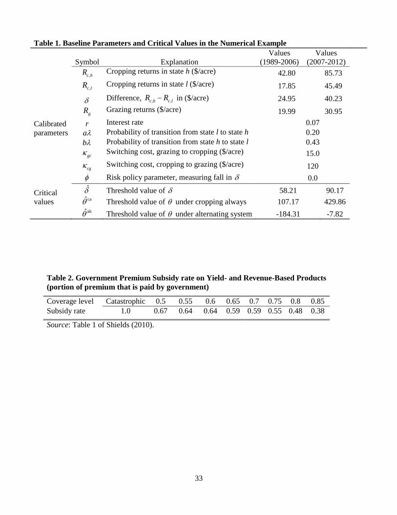
choices of each in turn. Table 1 summarizes values of these parameters in the baseline scenario
where there is no policy intervention (i.e., 0 ). Since crop prices increased dramatically in
2007 and thereafter, for returns parameters we calibrate two sets of values. One is for the
period before 2007 and the other is for the period 2007-2012.
Profitability level parameters
Returns from cropping (i.e., ,c hR and ,c lR ) in period 1989-2006 are calibrated by use of North
Dakota State University Extension annual crop budgets for the South Central North Dakota
(SCND) region.4 The SCND region contains 11 counties: Barnes, Dickey, Eddy, Foster,
Griggs, Kidder, LaMoure, Logan, McIntosh, Stutsman, and Wells (see the map in Figure SM1
of the Supplement Materials).5 We also calibrate a second set of cropping returns for the 2007-
2012 period as returns on cropping starting from 2007 were so high that the cropping
profitability clearly had entered in a new regime. From the crop budgets we collect returns to
land, labor, and management from growing corn, soybean, and wheat in each year. Then we
calculate a weighted average return for each year by using harvested acres in the South Central
North Dakota region as weights. The U.S. GDP implicit price deflator is used to translate the
returns into 2006 dollars. Returns in this article are all in 2006 dollars unless stated otherwise.
Figure 4 depicts the weighted average returns over 1989-2012.
4 Paulann Haakenson at North Dakota State University Extension Service generously shared the
historical crop budgets with us. 5 In 2005 and after, the SCND was redefined to contain only 6 counties: Burleigh, Emmons,
Kidder, Logan, McIntosh and Sheridan counties. Since a) the newly defined SCND is
geographically similar to the previously defined SCND; and b) the redefinition occurred at the
very end of our 1989-2006 regime, we assume that this regional redefinition does not affect the
underlying data generating mechanism to the parameters.

19
Since there is no clear upward trend in returns over 1989-2006, we use the sample mean of
the weighted average returns (i.e., $27.55/acre) as a threshold to differentiate returns in state h
and returns in state l.6 That is, if in a year the return is higher (respectively, lower) than the
sample mean, then we assume that state h (respectively, l) occurs in that year. By doing so we
transform the return process over 1989-2006 to a two-state process. If we label state h as 1 and
state l as 0, then the Dickey-Fuller test (performed by Stata command “dfgls”) rejects the null
hypothesis that the two-state process is a unit root.7 Moreover, the Kwiatkowski-Phillips-
Schmidt-Shin (KPSS) test on the two-state process does not reject the hypothesis that the process
is stationary at any reasonable significance level. We perform the same tests on the original
return process and the test results do not reject the stationarity hypothesis either. We then define
the simple average of returns in state h to be , ,c hR which is $42.8/acre. Similarly, we define
average returns in state l to be , ,c lR which is $17.85/acre. In the 2007-2012 regime, the cropping
returns in states h and l are $85.73/acre and $45.49/acre, respectively.
Returns from grazing, ,gR are calculated by using pasture cash rent in North Central South
Dakota over 1991-2006 because pasture cash rent data in South Central North Dakota are not
available to us.8 We first translate the cash rent into 2006 dollars and then let the returns from
grazing, ,gR equal the cash rent average, or $19.99/acre. In the 2007-2012 regime, returns from
grazing equal $30.95/acre.
Dynamic parameters
We apply maximum likelihood methods to estimate the transition probabilities between state h
6 A simple ordinary least square regression of the weighted average returns on year shows that
the coefficient on year is insignificant (with p-value at 0.28). 7 The same results are obtained when we perform the Phillips-Perron unit-root test by using Stata
command “pperron” and when we perform the augmented Dickey-Fuller unit-root test by using
Stata command “dfuller.” 8 The counties in the North Central South Dakota area are Brown, Campbell, Edmunds, Faulk,
McPherson, Potter, Spink, and Walworth (see the map in Figure SM1 of the Supplemental
Materials).
20
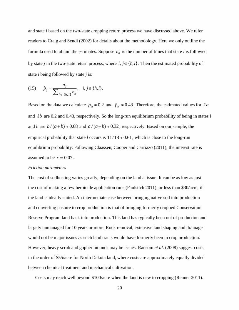
and state l based on the two-state cropping return process we have discussed above. We refer
readers to Craig and Sendi (2002) for details about the methodology. Here we only outline the
formula used to obtain the estimates. Suppose ijn is the number of times that state i is followed
by state j in the two-state return process, where ,, { }.hi lj Then the estimated probability of
state i being followed by state j is:
(15)
{ , }
, , { , .ˆ }ij
ij
ij
j h l
np
ni j h l
Based on the data we calculate ˆ 0.2lhp and 0.43ˆhlp . Therefore, the estimated values for a
and b are 0.2 and 0.43, respectively. So the long-run equilibrium probability of being in states l
and h are / ( ) 0.68b a b and / ( ) 0.32a a b , respectively. Based on our sample, the
empirical probability that state l occurs is 11/18 0.61 , which is close to the long-run
equilibrium probability. Following Claassen, Cooper and Carriazo (2011), the interest rate is
assumed to be 0.07r .
Friction parameters
The cost of sodbusting varies greatly, depending on the land at issue. It can be as low as just
the cost of making a few herbicide application runs (Faulstich 2011), or less than $30/acre, if
the land is ideally suited. An intermediate case between bringing native sod into production
and converting pasture to crop production is that of bringing formerly cropped Conservation
Reserve Program land back into production. This land has typically been out of production and
largely unmanaged for 10 years or more. Rock removal, extensive land shaping and drainage
would not be major issues as such land tracts would have formerly been in crop production.
However, heavy scrub and gopher mounds may be issues. Ransom et al. (2008) suggest costs
in the order of $55/acre for North Dakota land, where costs are approximately equally divided
between chemical treatment and mechanical cultivation.
Costs may reach well beyond $100/acre when the land is new to cropping (Renner 2011).

21
In addition to rock, scrub and perhaps fence removal, gulleys and gopher holes may need to be
filled. Labor may be a significant component of cost. In this article we focus on how risk
interventions and switching cost reductions can affect the critical value of at which land
value is unaffected by the sodbusting decision. Since we have very limited information on the
distribution of , we utilize the change in the critical value of to roughly measure the
grassland-conversion impact of risk interventions and switching cost reductions.
The cost of switching from well-maintained pasture to cropping is typically not large,
where tilling and herbicide are the most prominent parts. Therefore, we assume that gc
$15 / acre . The cost of establishing a pasture is typically much larger. For Iowa, Barnhart and
Duffy (2012) assert a cost of about $200/acre depending on cultivation, weed management,
seeding and fertilization choices. For North Dakota, with generally less productive land,
growers are not likely to pay that much and we assume a cost of $120 / acrecg for
conversion.
Policy parameter
Table 2 provides premium subsidy rates that were available on the most popular government
yield and revenue insurance contracts in 2012. Catastrophic insurance is provided free for
losses beyond 50% of expected yield or revenue where yield expectations are computed from
historical yield data. Typical coverage levels chosen vary with crop and location but are
broadly about 70% or more, so that subsidies are in the range of 38-59%. In the simulation we
calibrate as the ratio of crop insurance subsidy over cropping return shortfall, . Since an
actuarially fair insurance does not affect expected net returns, it is the crop insurance subsidy
that matters for land-owners’ expected returns.
The crop insurance subsidy is calculated as the average of per acre subsidy in North Dakota
over 1989-2006, which is $4.9/acre. The state-level of crop insurance subsidy and insured
acres over 1989-2006 is obtained from Summary of Business Reports and Data of Risk

22
Management Agency (RMA) at USDA.9 We calculate that over the 1989-2006 regime
4.9 / 24.95 0.2 . In the simulation, to check sensitivity we also vary the value of from 0.2.
In the 2007-2012 regime, the subsidy over cropping returns shortfall ratio is about 0.5. In the
baseline scenario where there is no policy intervention we let 0.
Simulations
We are interested in examining how a) implementation of a policy that directly modifies the
cropping return shortfall, , and b) technology advances that reduce switching cost between
cropping and grazing, i.e., cg and gc , would affect land use. Therefore, we need to identify
how the critical values of cropping return shortfall, , and the one-time sod-busting cost, ,
are affected by the risk intervention policy and technology advances. Table 1 lists these critical
values in the baseline scenario under which there is no policy intervention (i.e., 0 ). From
eqn. (7), ˆ $58.21/ acre over the 1989-2006 regime while ˆ $90.17 / acre over the 2007-
2012 regime. Since the baseline scenario is $24.95/acre (respectively, $40.23/acre) under
the 1989-2006 (respectively, 2007-2012) regime, we know that were a parcel of native sod
converted then it would be under ‘crop always’ rather than ‘alternate’.
In the baseline scenario , the critical value for the one-time sod-busting cost in 1989-2006
is $107.17/acre (Table 1), implying that native sod with one-time conversion cost lower than
$107.17/acre will be converted into the ‘crop always’ system. In the 2007-2012 regime the
critical value becomes $429.86/acre in the baseline scenario (Table 1). We can see that in the
2007-2012 regime under the baseline scenario, the critical value of is about four times as
large as that in the 1989-2006 regime, which means that higher cropping returns in the 2007-
2012 regime significantly increases the critical values of sod-busting cost at which landowners
are indifferent between converting and not converting. In both regimes, the critical values of
9 Link: http://www.rma.usda.gov/data/sob.html.

23
under ‘alternate’ are negative, which means that were ˆ then native sod would not be
converted even if the sod-busting cost were zero.
Tables 3 and 4 present simulation results of critical values of and upon risk
intervention and decreasing switching costs in the 1989-2006 and 2007-2012 regimes,
respectively. There are three panels in each of Tables 3 and 4. The first column in each panel
includes the critical values of and in the baseline scenario (i.e., 0 , 15gc , and
120cg ). In both regimes, a risk intervention significantly increases the critical values of
sod-busting cost. For example, consider the 1989-2006 regime. When the reduction in cropping
returns shortfall is 20% (i.e., 0.2 , the calibrated value) then, compared with the baseline
scenario, the critical value of sod-busting cost (i.e., ca ) will increase from $107.17/acre to
$150.91/acre, which is a 41% increase (see Panel A of Table 3). Even a 10% reduction in
shortfall (i.e., 0.1 ) will increase ca by 20%. The critical values of return shortfall, , are
increased by risk intervention as well. When 0.2 and when compared with the value in the
baseline scenario, then abs increases from $58.21/acre to $72.76/acre, a 25% increase (see
Panel B of Table 3). So the crop insurance subsidy makes it more likely that native sod will be
converted into ‘crop always’.
In the 2007-2012 regime, the calibrated risk intervention parameter (i.e., 0.5 ) is much
higher than that in regime 1989-2006. When 0.5 then the absolute increase in ca is as
large as $176/acre (calculated by using 606.17 429.86 from Panel A of Table 4). However,
in the 2007-2012 regime the calibrated risk intervention (i.e., 0.5 ) increases abs by 100%
when compared with the baseline scenario, which makes the converted native sod more likely
under ‘crop always’ system (see Panel A of Table 4).
On the other hand the effects of a decrease in switching costs, cg or gc , are much smaller

24
in magnitude than the effects of a risk policy adjustment. In the 1989-2006 regime, we can see
that when the switching cost from grazing to cropping (i.e., gc ) decreases from $15/acre to
$3/acre then a) abs only decreased by $2.4/acre, and b) the critical value of sod-busting cost
under the ‘alternate’ system, alt , remains negative (see Panel B of Table 3). Regarding the
impacts of a decrease in the cost of switching from cropping to grazing (i.e., cg ), similar
conclusions can be made except that when cg reaches $40/acre then alt becomes positive
(see Panel C of Table 3). In the 2007-2012 regime the effects of decreasing switching costs are
not significant either. When switching costs are zero (i.e., 0gc cg ), however, then native
sod will be converted into the ‘alternate' system under the 1989-2006 regime and into the ‘crop
always’ system under the 2007-2012 regime (upper rows in Table 5).
One may be interested in the critical values of sod-busting costs when the landowner omits
risks in cropping returns. That is, the landowner converts native sod whenever the net present
value of long-run equilibrium expected cropping returns is greater than the sum of conversion
cost and the net present value of grazing returns. This is of interest because studies on
grassland conversion typically base their methodologies on this idea. Examples include
Claassen, Cooper and Carriazo (2011), Claassen et al. (2011), and Rashford, Walker, and
Bastian (2011).
The lower rows in table 5 show that in the 1989-2006 regime ca 8 82ˆ 2. when ,c hR and
,c lR are set to equal $25.79/acre, the long-run equilibrium expected cropping returns over the
period. Clearly here the value of ca is 23% (or $24.35/acre) smaller than that in the baseline
scenario, which is $107.17/acre. In other words, omission of cropping return risk across
periods will lead to an underestimation of the magnitude of grassland conversions. The reason
is as follows. Sod-busting always occurs in state h. Moreover, state h will persist at time t with

25
approximate probability 1 bt . Therefore, if the interest rate is greater than 0 (i.e., the
discount factor is less than 1), then the present value of long-run equilibrium expected returns
is less than the present value of land under the ‘crop always’ system. That is, omission of risk
across periods will underestimate expected net returns from cropping, and hence underestimate
the magnitude of grass conversions. Of course, if the interest rate is 0 (i.e., the discount factor
equals 1) then the present value of long-run equilibrium expected returns is equal to the present
value of the ‘crop always’ system.
Conclusion
Under a two-point Markov random return process, we have developed and simulated a real
option model that articulates incentives arising from cultivation innovations and changes in the
risk management subsidy policy environment surrounding crop production. We have shown
that, upon plowing, native sod is followed by either i) a ‘crop always’, i.e., permanent
cropping, or ii) an ‘alternate’ system, in which land is put under cropping (respectively,
grazing) whenever crop prices are high (respectively, low). We then compared the value of
land under these two systems with the value of land under native sod having accounted for the
switching costs incurred upon alternating between cropping and grazing. In this comparison we
studied how a) risk interventions and b) cropping innovations that reduce switching costs affect
a landowner’s sod-busting decision. Our findings were that the presence of risk intervention
likely converts marginal native sod to a ‘crop always’ rather than an ‘alternating’ production
system. For land that has already been converted, a risk management intervention would
increase the fraction of land tracts under a ‘crop always’ system while decreasing the fraction
under an ‘alternate’ system. Theoretically, cropping innovations that reduce switching costs
will reduce the extent of native sod land tracts and land originally under a ‘crop always’ system
and increase the extent of land under an ‘alternate’ system.
Based on data from South Central North Dakota, the calibrated model shows that risk

26
policy interventions would likely have more significant effects on native sod conversion than
would innovations in switching costs. Consider a risk intervention that causes a 20% reduction
in the extent to which cropping returns fall short of their potential. This intervention would
increase the maximum (or threshold) value of the one-time sod-busting cost that an asset value
maximizing land owner would pay by 41%, or $43.7/acre, under the 1989-2006 regime.
Although we cannot quantify the magnitude of native sod that would be affected by this
increase in threshold value without knowing the distribution of sod-busting costs, we believe
that the 41% increase indicates a significant change in motivation for native sod conversion.
Our simulation also shows that omitting cropping returns risk across time underestimates the
threshold value of sod-busting cost by 23% and hence underestimates the incentive for native
sod conversion to crop production.
References
Alston, J.M., J.M. Beddow, and P.G. Pardey. 2009. “Agricultural Research, Productivity, and
Food Prices in the Long Run.” Science, 325(5945):1209-1210.
Badh, A., A. Akyuz, G. Vocke, and B. Mullins. 2009. “Impact of Climate Change on the
Growing Season in Selected Cities of North Dakota, United States of America.” The
International Journal of Climate Change: Impacts and Responses, 1(1):105-118.
Barnhart, S., and M. Duffy. 2012. “Estimated Costs of Pasture and Hay Production.” Iowa State
University Extension Publication Ag-96, File A1-15, March.
Claassen, R., F. Carriazo, J.C. Cooper, D. Hellerstein, and K. Ueda. 2011. “Grassland to
Cropland Conversion in the Northern Plains.” U.S. Department of Agriculture, Economic
Research Report No. 120, June.
Claassen, R., J.C. Cooper, and F. Carriazo. 2011. “Crop Insurance, Disaster Payments, and Land
Use Change: The Effect of Sodsaver on Incentives for Grassland Conversion.” Journal of

27
Agricultural and Applied Economics, 43(2):195-211.
Craig, B.A., and P.P. Sendi. 2002. “Estimation of the Transition Matrix of a Discrete-time
Markov Chain.” Health Economics, 11(1):33-42.
Deaton, A., and G. Laroque. 1992. “On the Behavior of Commodity Prices.” Review of
Economic Studies, 59(1):1-23.
Dixit, A. 1989. “Entry and Exit Decisions under Uncertainty.” Journal of Political Economy,
97(3):620-638.
Doole, G.J., and G.L. Hertzler. 2011. “Optimal Dynamics Management of Agricultural Land-
Uses: An Application of Regime Switching.” Journal of Agricultural and Applied
Economics, 43(1):43-56.
Duke, S.O., and S.B. Powles. 2009. “Glyphosate-resistant Crops and Weeds: Now and in the
Future.” AgBioForum, 12(3&4):346-357.
Enders, E., and M.T. Holt. 2012. “Sharp Breaks or Smooth Shifts? An Investigation of the
Evolution of Primary Commodity Prices.” American Journal of Agricultural Economics,
94(3):659-673.
Faulstich, J. 2011. “Opportunities for Grassland Conservation.” Oral presentation at America’s
Grasslands: Status, Threats, and Opportunities Conference, Sioux Falls, SD, August 15-17,
2011.
Ghoshray, A. 2013. “Dynamic Persistence of Primary Commodity Prices.” American Journal
of Agricultural Economics, 95(1):153-164.
Glauber, J.W. 2013. “The Growth of the Federal Crop Insurance Program, 1990-2011.”
American Journal of Agricultural Economics, 95(2):482-488.
Goodwin, B.K., M.L. Vandeveer, and J.L. Deal. 2004. “An Empirical Analysis of Acreage
Effects of Participation in the Federal Crop Insurance Program.” American Journal of
Agricultural Economics, 86(4):1058-1077.

28
Governmental Accounting Office (GAO). 2007. “Farm Program Payments are an Important
Factor in Landowners’ Decisions to Convert Grassland to Cropland.” GAO report number
GAO-07-1054, September.
Hennessy, D.A. 2006. “On Monoculture and the Structure of Crop Rotations.” American Journal
of Agricultural Economics, 88(4):900-914.
Hertzler, G.L. 1990. “Dynamically Optimal Adoption of Farming Practices which Degrade or
Renew the Land.” Agricultural Economics Discussion Paper No 5/90, University of Western
Australia, Perth.
Hoel, P.G., S.C. Port, and C.J. Stone. 1972. Introduction to Stochastic Processes. Boston, MA:
Houghton Mifflin.
Johnston, C. 2012. “Cropland Expansion into Prairie Pothole Wetlands, 2001-2010.” In A.
Glaser, ed. America’s Grasslands: Status, Threats, and Opportunities. Proceedings of the 1st
Biennial Conference on the Conservation of America’s Grasslands. Sioux Falls SD, 15-17
August, 2011, pp. 44-46.
Kucharik, C.J. 2006. “A Multidecadal Trend of Earlier Corn Planting in the Central USA.”
Agronomy Journal, 98(6):1544-1550.
Kucharik, C.J. 2008. “Contributions of Planting Date Trends to Increased Maize in the Central
United States.” Agronomy Journal, 100(2):328-336.
Lubowski, R.N., S. Bucholtz, R. Claassen, M.J. Roberts, J.C. Cooper, A. Gueorguieva, and R.
Johansson. 2006. “Environmental Effects of Agricultural Land-Use Change: the Role of
Economics and Policy.” U.S. Department of Agriculture, Economic Research Report No. 25.
McConnell, K.E. 1983. “An Economic Model of Soil Conservation.” American Journal of
Agricultural Economics, 65(1):83-89.
Nail, E.L., D.L. Young, and W.F. Schillinger. 2007. “Diesel and Glyphosate Price Changes
Benefit the Economics of Conservation Tillage versus Traditional Tillage.” Soil and Tillage

29
Research, 94(2):321-327.
Rashford, B.S., J.A. Walker, and C.T. Bastian. 2011. “Economics of Grassland Conversion to
Cropland in the Prairie Pothole Region.” Conservation Biology, 25(2):276-284.
Ransom, J., D. Aakre, D. Franzen, H. Kandel, J. Knodel, J. Nowatzki, K. Sedivec, and R.
Zollinger. 2008. “Bringing Land in the Conservation Reserve Program Back into Crop
Production or Grazing.” North Dakota State University Extension Publication A-1364, June.
Renner, Dennis. 2011. Personal communication with Morton County, North Dakota, rancher and
crop producer. Mandan Natural Resources Conservation Building, North Dakota, November
1.
Setiyono, T.D., H. Yang, D.T. Walters, A. Dobermann, R.B. Ferguson, D.F. Roberts, D.J. Lyon,
D.E. Clay, and K.G. Cassman. 2011. “Maize-N: A Decision Tool for Nitrogen Management
in Maize.” Agronomy Journal, 103(4):1276-1283.
Shields, D.A. 2010. Federal Crop Insurance: Background and Issues. Congressional Research
Service. CRS Report for Congress, December 13.
Smith, V.H. 2011. “Premium Payments: Why Crop Insurance Costs too Much.” American
Enterprise Institute, July 12.
Stephens, S.E., J.A. Walker, D.R. Blunk, A. Jayaraman, D.E. Naugle, J.K. Ringleman, and A.J.
Smith. 2008. “Predicting Risk of Habitat Conversion in Native Temperate Grasslands.”
Conservation Biology, 22(5):1320-1330.
Stubbs, M. 2007. “Land Conversion in the Northern Plains.” Congressional Research Service,
April 5.
Tollefson, J. 2011. “Drought-tolerant Maize gets U.S. Debut.” Nature, 469(January 13):144-144.
Trigeorgis, L. 1996. Real Options: Managerial Flexibility and Strategy in Resource Allocation.
Cambridge, MA: MIT Press.
Triplett Jr., G.B., and W.A. Dick. 2008. “No-Tillage Crop Production: A Revolution in

30
Agriculture.” Agronomy Journal, 100(3 Supplement):S153-S165.
United States Department of Agriculture (USDA). 1997. Usual Planting and Harvesting Dates
for U.S. Field Crops. National Agricultural Statistics Service, Agricultural Handbook No.
628, December.
United States Department of Agriculture (USDA). 2010. Field Crops: Usual Planting and
Harvesting Dates. National Agricultural Statistics Service, Agricultural Handbook No. 628,
October.
Willassen, Y. 2004. “On the Economics of the Optimal Fallow-Cultivation Cycle.” Journal of
Economics Dynamics and Control, 28(8):1541-1556.
Wright, C.K. and M.C. Wimberly. forthcoming. “Recent Land Use Change in the Western
Corn Belt Threatens Grasslands and Wetlands.” Proceedings of the National Academy of
Sciences of the United States of America. Published online before print: doi:
10.1073/pnas.1215404110
Young, C.E., M. Vandeveer, and R. Schnepf. 2001. “Production and Price Impacts of U.S. Crop
Insurance Programs.” American Journal of Agricultural Economics, 83(5):1196-1203.
Yu, T., and B.A. Babcock. 2010. “Are U.S. Corn and Soybeans Becoming More Drought
Tolerant?” American Journal of Agricultural Economics, 92(5):1310-1323.
Appendix A
In this appendix we derive equation system (1). Following standard Bellman equation
statistical methods, if one commences in state h then
(A1) ,( ;ca) (1 ) [ | ]c h th R t rt E h
where ,c hR t is income over a small immediate time interval, 1 rt is the locally valid
approximation of the time discount factor and [ | ]tE h is the present time expectation of value
after time increment t given that the initial state is h.

31
In turn,
(A2) [ | ] ( ;ca) (1 ) ( ;ca)tE h bt l bt h
where i) ( ;ca)bt l is the product of the approximate probability of state change and value
under the state change while ii) (1 ) ( ;ca)bt h is the product of the approximate probability
of state continuance and value under continuance. Insert (A2) into (A1) to obtain
(A3) ,( ;ca) (1 ) ( ;ca) (1 ) ( ;ca)c hh R t rt bt l bt h
and so, upon some housekeeping,
(A4) , (1 ) ( ;ca)
( ;ca) .c hR rt b lh
r b r bt
Taking the infinitesimal limit, so that the approximation converges to equality, we have
(A5) , ,
0
(1 ) ( ;ca) ( ;ca)Lim
c h c h
t
R rt b l R b l
r b r bt r b
so that ,( ;ca) [ ( ;ca)] / ( )c hh R b l r b and
(A6) ,( ;ca) [ ( ;ca) ( ;ca)].c hr h R b l h
A similar argument can be used to establish that, upon commencing in state l, then
(A7) ,( ;ca) [ ( ;ca) ( ;ca)].c hr l R a h l
Now write out system (A6)-(A7) as
(A8) ,
,
( ;ca).
( ;ca)
c h
c h
Rb r b l
Rr a a h
Invert to obtain system (1).
Appendix B
In this appendix we derive equation system (4). Instead of equation (A3) and the corresponding
equation for the l state, the state equations are

32
(B1)
,( ;alt) (1 ) [ ( ;alt) ] (1 ) ( ;alt) ;
( ;alt) (1 ) [ ( ;alt) ] (1 ) ( ;alt) .
c h cg
g gc
h R t rt bt l bt h
l R t rt at h at l
Here the state h value factors in ( ;alt) cgl because this is the value upon incurring pasture
establishment cost cg under state transition from h to l. The state l value factors in
( ;alt) gch because the state transition from l to h involves incurring the pasture
termination cost gc . Upon some housekeeping, we have
(B2)
, (1 ) [ ( ;alt) ]( ;alt) ;
(1 ) [ ( ;alt) ]( ;alt) .
c h cg
g gc
R rt b lh
r b r bt
R rt a hl
r a rt a
Taking the infinitesimal limit in each case allows us to arrive at
(B3)
, ,
0
0
(1 ) [ ( ;alt) ] [ ( ;alt) ]Lim ( ;alt);
(1 ) [ ( ;alt) ] [ ( ;alt) ]Lim ( ;alt).
c h cg c h cg
t
g gc g gc
t
R rt b l R b lh
r b r bt r b
R rt a h R a hl
r a rt a r a
Now write out system (B3) as
(B4) ,( ;alt)
,( ;alt)
c h cg
g gc
R bb r b l
R ar a a h
and invert:
(B5)
,
,
( ) ( )( )( ;alt) ;
( )
( )( ) ( )( ;alt) .
( )
c h cg g gc
c h cg g gc
a R b r b R al
r r a b
r a R b b R ah
r r a b
Then utilize equation system (1), to obtain system (4).
33
Table 2. Government Premium Subsidy rate on Yield- and Revenue-Based Products
(portion of premium that is paid by government)
Coverage level Catastrophic 0.5 0.55 0.6 0.65 0.7 0.75 0.8 0.85
Subsidy rate 1.0 0.67 0.64 0.64 0.59 0.59 0.55 0.48 0.38
Source: Table 1 of Shields (2010).
Table 1. Baseline Parameters and Critical Values in the Numerical Example
Symbol Explanation
Values
(1989-2006)
Values
(2007-2012)
,c hR Cropping returns in state h ($/acre) 42.80 85.73
,c lR Cropping returns in state l ($/acre) 17.85 45.49
Difference, , ,c h c lR R in ($/acre) 24.95 40.23
Calibrated
parameters
gR Grazing returns ($/acre) 19.99 30.95
r Interest rate 0.07
a Probability of transition from state l to state h 0.20
b Probability of transition from state h to state l 0.43
gc Switching cost, grazing to cropping ($/acre) 15.0
cg Switching cost, cropping to grazing ($/acre) 120
Risk policy parameter, measuring fall in 0.0
Critical
values
Threshold value of 58.21 90.17 ca Threshold value of under cropping always 107.17 429.86
alt Threshold value of under alternating system -184.31 -7.82

34
Table 4. Dollar Critical Values of and under Risk Interventions or under
Changes in Switching Costs (2007-2012 Regime)
Panel A: critical values of and when increases
0 (baseline) 0.45 0.50 0.55 0.60
abs 90.17 163.95 180.35 200.39 225.43 ca 429.86 588.54 606.17 623.80 641.43 alt -7.82 -7.82 -7.82 -7.82 -7.82
Panel B: critical values of and when gc decreases
15gc (baseline) 12gc 9gc 6gc 3gc
abs 90.17 89.57 88.97 88.37 87.77 ca 429.86 429.86 429.86 429.86 429.86 alt -7.82 -2.56 2.70 7.95 13.21
Panel C: critical values of and when cg decreases
120cg (baseline) 100cg 80cg 60cg 40cg
abs 90.17 84.77 79.37 73.97 68.57 ca 429.86 429.86 429.86 429.86 429.86 alt -7.82 39.51 86.83 134.16 181.49
Table 3. Critical Values of and under Risk Interventions or under Changes in
Switching Costs (1989-2006 Regime)
Panel A: critical values of and when increases
0 (baseline) 0.1 0.15 0.2 0.25
abs 58.21 64.68 68.48 72.76 77.61 ca 107.17 129.04 139.97 150.91 161.84 alt -184.31 -184.31 -184.31 -184.31 -184.31
Panel B: critical values of and when gc decreases
15gc (baseline) 12gc 9gc 6gc 3gc
abs 58.21 57.60 57.00 56.40 55.80 ca 107.17 107.06 107.06 107.06 107.06 alt -184.31 -179.09 -173.84 -168.58 -163.32
Panel C: critical values of and when cg decreases
120cg (baseline) 100cg 80cg 60cg 40cg
abs 58.21 52.80 47.40 42.00 36.60 ca 107.17 107.06 107.06 107.06 107.06 alt -184.31 -137.03 -89.70 -42.37 4.95

35
Table 5. Dollar Critical Values of and under No Risk (i.e., , ,c h c lR R ) or under
Zero Switching Costs (i.e., 0gc cg )
Regime ,c hR ,c lR gR abs ca
alt
No switching
cost
1989-2006 42.80 17.85 19.99 22.81 107.17 125.94
2007-2012 85.73 45.49 30.95 54.77 429.86 302.43
No risk in
Returns
1989-2006 25.79 25.79 19.99 41.20 82.82 -278.24
2007-2012 58.29 58.29 30.95 62.74 390.59 -159.29
Figure 1. Sodbusting choices in (δ, θ) space
δ
θ
0
altca-con 0h
Keep in native sod
Convert and
choose ‘crop
always’ system
Convert and choose
‘alternate’ system
alt-con 0h
,( ) /c h gR R r

36
Figure 2. Effect of risk intervention on sodbusting
choices in (δ, θ) space
δ
θ
0
ca-con 0h
Keep in native sod
Convert to
‘crop always’
Convert to
‘alternate’
alt-con 0h
,c h gR R
r
abs
,abs
ca-con 0h
A
B
alt
Figure 3. Effect of lower grass to crop conversion
cost on sodbusting choices in (δ, θ) space
δ
θ
0
ca-con 0h
Keep in native sod
Convert to
‘crop always’
Convert to
‘alternate’
alt-con 0h
,c h gR R
r
DC
alt
alt

37
0
20
40
60
80
100
120
198919911993199519971999200120032005200720092011
Year
Cro
ppin
g R
etu
rns
($/a
cre)
2006
Figure 4. Cropping Returns over 1989-2012 in South Central North
Dakota (in 2006 dollars)

1
Supplemental Materials
Item A
In this item we show that once sod is busted then the land owner will either ‘crop always’ or
‘alternate’. In ‘crop always’ the land owner always crops regardless of the state of nature. In
the ‘alternate’ system the land owner crops under state h but grazes under state l.
Let the moment when native sod is busted be denoted as time 0. At each time 0t the
landowner considers whether to take action ‘crop’ (labeled as c) or ‘graze’ (labeled as g), based
on i) the current state of nature (i.e., h and l) and ii) the current state of land-use (i.e., cropping
or grazing). The current state of land-use at time t should be taken into account when choosing
an action at time t because a switching cost will be incurred whenever the landowner switches
land-use from one type to the other. Since nature’s state change occurs in a Markovian
continuous time setting, only the current state matters for the time t decision. Therefore, the
landowner has sixteen strategies for choosing a land-use type at time t. Let “(i, j) k” stand
for “if nature’s state is { , }i h l and if the land is currently under land-use type { , }j c g , then
the landowner chooses land-use type { , }k c g at time t.”
The sixteen strategies can be written as:
1) (h, c) c, (h, g) c, (l, c) c, (l, g) c;
2) (h, c) c, (h, g) c, (l, c) c, (l, g) g;
3) (h, c) c, (h, g) c, (l, c) g, (l, g) c;
4) (h, c) c, (h, g) c, (l, c) g, (l, g) g;
5) (h, c) c, (h, g) g, (l, c) c, (l, g) c;
6) (h, c) c, (h, g) g, (l, c) c, (l, g) g;
7) (h, c) c, (h, g) g, (l, c) g, (l, g) c;
8) (h, c) c, (h, g) g, (l, c) g, (l, g) g;
9) (h, c) g, (h, g) c, (l, c) c, (l, g) c;
10) (h, c) g, (h, g) c, (l, c) c, (l, g) g;
11) (h, c) g, (h, g) c, (l, c) g, (l, g) c;
12) (h, c) g, (h, g) c, (l, c) g, (l, g) g;
2
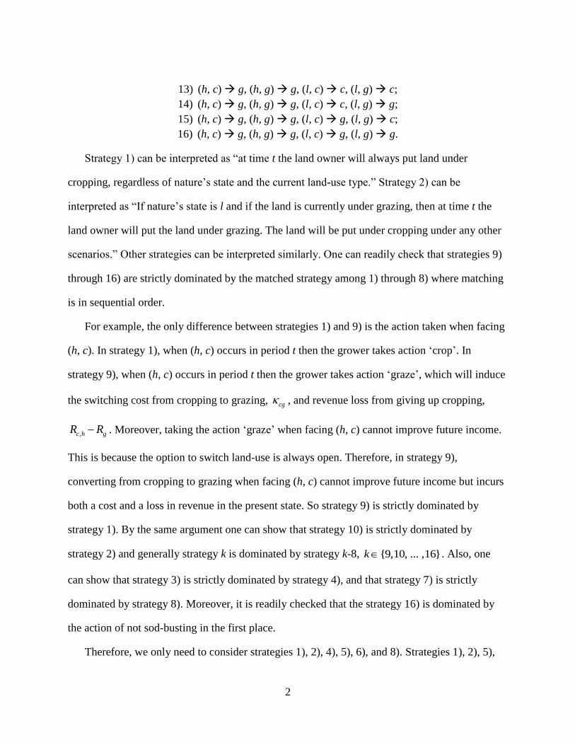
13) (h, c) g, (h, g) g, (l, c) c, (l, g) c;
14) (h, c) g, (h, g) g, (l, c) c, (l, g) g;
15) (h, c) g, (h, g) g, (l, c) g, (l, g) c;
16) (h, c) g, (h, g) g, (l, c) g, (l, g) g.
Strategy 1) can be interpreted as “at time t the land owner will always put land under
cropping, regardless of nature’s state and the current land-use type.” Strategy 2) can be
interpreted as “If nature’s state is l and if the land is currently under grazing, then at time t the
land owner will put the land under grazing. The land will be put under cropping under any other
scenarios.” Other strategies can be interpreted similarly. One can readily check that strategies 9)
through 16) are strictly dominated by the matched strategy among 1) through 8) where matching
is in sequential order.
For example, the only difference between strategies 1) and 9) is the action taken when facing
(h, c). In strategy 1), when (h, c) occurs in period t then the grower takes action ‘crop’. In
strategy 9), when (h, c) occurs in period t then the grower takes action ‘graze’, which will induce
the switching cost from cropping to grazing, cg , and revenue loss from giving up cropping,
,c h gR R . Moreover, taking the action ‘graze’ when facing (h, c) cannot improve future income.
This is because the option to switch land-use is always open. Therefore, in strategy 9),
converting from cropping to grazing when facing (h, c) cannot improve future income but incurs
both a cost and a loss in revenue in the present state. So strategy 9) is strictly dominated by
strategy 1). By the same argument one can show that strategy 10) is strictly dominated by
strategy 2) and generally strategy k is dominated by strategy k-8, {9,10, ... ,16}k . Also, one
can show that strategy 3) is strictly dominated by strategy 4), and that strategy 7) is strictly
dominated by strategy 8). Moreover, it is readily checked that the strategy 16) is dominated by
the action of not sod-busting in the first place.
Therefore, we only need to consider strategies 1), 2), 4), 5), 6), and 8). Strategies 1), 2), 5),

3
and 6) are equivalent to the ‘crop always’ system. This is because sod-busting only occurs under
state h and whenever the sod is busted then it is converted to cropland. That is, at time 0t we
have (h, c). Therefore, starting from time 0t , if the landowner follows strategies 1), 2), 5), and
6), then ‘grazing’ will never occur in the system, which implies the ‘crop always’ system.
Similarly, starting from time 0t if the landowner follows strategy 4), then the land will be
under cropping (respectively, grazing) whenever the state is h (respectively, l), which implies the
‘alternate’ system. Were the native sod busted, then strategy 8) would never be optimal. The
reason is as follows. If the native sod is busted, then busting is profitable when nature’s state is h.
Suppose strategy 8) is followed after the sod is busted and suppose the system evolves to (h, g),
or the situation in which nature’s state is h and the current land use is grazing. In this situation,
deviating from strategy 8) (i.e., putting land under cropping) will be more profitable than
following strategy 8) because under state h busting native sod has been profitable. Recall that the
one-time sod-busting cost, , is higher than the switching cost from grazing to cropping, gc .
In sum, once native sod has been converted then we only need to consider the ‘crop always’
and ‘alternate’ systems. At no loss we may represent ‘crop always’ and ‘alternate’ by strategies
1) and 4), respectively.

4
Meade
Butte
Dunn
Perkins
Ward
Dewey
Cass
CorsonHarding
Grant
McLeanMcKenzie
Morton
Brown
Spink
Day
Hand
Williams
Stark
Ziebach
Stutsman
Wells
Haakon
Kidder
Sully
Slope
Barnes
MountrialWalsh
Divide
Sioux
Stanley
Burke
Clark
Benson
Faulk
CavalierBottineau
Beadle
Traill
Dickey
Logan
Mercer
Ramsey
Pennington
Potter
AdamsBowman
Eddy
Oliver
Grant
Hettinger La Moure
Edmunds
SargentMcIntosh
Hughes
Foster
McHenry
Burleigh
Emmons
Pierce
Richland
Hyde
Billings
Nelson
Roberts
TownerRolette Pembina
Grand Forks
SheridanSteele
Renville
Griggs
Deuel
Ransom
MarshallMcPherson
KingsburyLawrence
Campbell
Brookings
Walworth
Hamlin
Golden Valley
Codington
Jones Lyman Buffalo LakeMiner
South Dakota
North Dakota
South Central
North Dakota
area*
North Central
South Dakota
area
Figure SM1. South Central North Dakota (SCND) area and North
Central South Dakota (NCSD) areaNote: * In 2005 and after, the SCND area was redefined to contain only 6 counties: Burleigh, Emmons,
Kidder, Logan, McIntosh and Sheridan counties.)