national parameters, economic opportunity cost of labor
TRANSCRIPT

National Parameters, Economic Opportunity Cost of Labor, Social Value of Time, and
Commodity-Specific Conversion Factors for Public Project Appraisal in Kenya
Summary Report Date: September 29, 2021 Submitted by: Cambridge Resources International, Inc. 1770Mass.Ave#617,Cambridge,MA02140,USA Phone: 1 (613) 770 2080 E-mail: [email protected] or [email protected]
In Consortium with: GEEKAN KENYA LTD RUPRANI HOUSE, MOKTAR DADAH P.O BOX 17460-00100 TEL:+254723729096 Email: [email protected] NAIROBI-KENYA. Presented to: THE MINISTRY OF NATIONAL TREASURY AND PLANNING, KENYA

Table of Contents
1. Introduction ............................................................................................................... 6
2. The Role of CSCFs in the Public Investment Management System. .................... 7
3. Moving from Financial Analysis to Economic Analysis ........................................ 7
4. The Role of National Parameters in Public Planning and Appraisal ................. 12
4.1. Economic Opportunity Cost of Capital ............................................................... 12
4.2. Foreign Exchange Premium and Premium for Non-Tradable Outlays ............... 13
5. Conclusion ................................................................................................................ 13
5.1. Recommendations ................................................................................................ 14
Annexure A: Kenya National Parameters Report ............................................................. 16
Annexure B: Estimation of Commodity-Specific Conversion Factors Report ................. 83
Annexure C: Economic Opportunity Cost of Labor ......................................................... 96
Annexure D: Social Value of Time ................................................................................. 133

ii
LIST OF ABBREVIATIONS
CF Conversion Factor
COMESA Common Market for Eastern and Southern Africa
CRI Cambridge Resources International Inc.
DSCR Debt Service Coverage Ratio
EAC East African Community
ENPV Economic Net Present Value
EOCK Economic Opportunity Cost of Capital
EOCL Economic Opportunity Cost of Labour
EPRA Energy and Petroleum Regulatory Authority
ERR Economic Rate of Return
FDI Foreign Direct Investment
FEP Foreign Exchange Premium
FIRR Financial Internal Rate of Return
FNPV Financial Net Present Value
FOB Free on Board
FTA Free Trade Agreement
GDP Gross Domestic Product
GFCF Gross Fixed Capital Formation
GVA Gross Value Added
HS Harmonized System (Harmonized Commodity and Coding System)
ICSD Investment and Capital Dataset
IGAD Intergovernmental Authority on Development

iii
IIA Integrated Investment Appraisal
IIR Internal Rate of Return
ILO International Labor Organization
IMF International Monetary Fund
KES Kenyan Shilling
KM Kilometer
LB Labour Benefits
LE Labour Externality
MDAs Ministries, Departments and Agencies
MIS Malaria Indicator Survey
NPV Net Present Value
NTP Non-Tradable Outlays
NTSA National Transport and Safety Authority
PV Present Value
ROE Return on Equity
RWG Real Growth Rate
SOEs State Owned Enterprises
SVT Social Value of Time
UNICEF United Nations Children's Emergency Fund
USD United States Dollars
VAT Value Added Tax
VIP Ventilated Improved Pit
WCO World Customs Organization

iv
TERMS AND DEFINITIONS
Business Cycle: Business cycles are intervals of expansion followed by a recession in economic activity. They have implications for the welfare of the broad population as well as for private institutions. Commodity Specific Conversion Factor: The ratio of the economic value of a commodity to its financial value.
Economic Opportunity Cost: The value of utility that can be derived were the same resources used in the next best alternative to the proposed project or programme.
Economic Resource Flow Statement: A statement used to organize and present the economic inflow and outflow of a project.
Financial Cash Flow Statement: A statement used to organize and present the project's financial cash flow structure. It is generally divided into two sections, the cash inflow, and the cash outflow.
Financial Intermediation: This is the process of transferring sums of money from economic agents with surplus funds to economic agents that would like to utilize those funds.
Foreign Exchange Premium (FEP): The proportion with which the economic exchange rate exceeds the market exchange rate.
Gross Fixed Capital Formation: Gross fixed capital formation is a macroeconomic concept used in official national accounts such as the United Nations System of National Accounts, National Income and Product Accounts, and the European System of Accounts. Statistically, it measures the value of new or existing fixed assets acquisitions by the business sector, governments, and "pure" households (excluding their unincorporated enterprises) fewer disposals of fixed assets. GFCF is a component of the expenditure on GDP and thus shows something about how much of the new value-added in the economy is invested rather than consumed. Harmonized System (HS): The Harmonized Commodity Description and Coding System, generally known as the Harmonized System (HS), is used by the World Customs Organization (WCO) as an internationally standardized system of names and numbers to classify traded products.
Infrastructure Investment Project: Spending on new assets; replacements; maintenance and repairs; upgrades and additions; and rehabilitation, renovation, and refurbishment of assets.
Integrated Investment Appraisal (IIA): A methodology of conducting investment appraisal that incorporates the financial, economic, stakeholder, and risk analyses of the project together.
National Parameters Database: A compilation of the national parameters and the commodity-specific conversion factors developed for Kenya.

v
Net Economic Benefit: The difference between the economic benefit and the resource cost (economic cost)
Newly Stimulated Household Savings: The new household savings stimulated by the increase in the demand for funds needed to finance the investment project.
Premium for Non-Tradable Outlays: The percentage difference between the financial and economic cost of outlays on non-tradables.
Non-Traded Goods (Non-Tradables): These are goods and services whose prices are not determined in the world market. Their prices are instead determined in the domestic markets.
Opportunity Cost of Funds: This is the expected return from the next best alternative foregone.
Project: A unique set of processes consisting of coordinated and controlled activities with start and end dates performed to achieve the project objective.
Real Value: The actual value of goods and services. It does not include the impact of inflation. Real values of goods and services are obtained from nominal values by adjusting for inflation.
Reproducible Remunerative Investment: Represents the remunerative portion of the total investment in six assets, i.e., structures, transport equipment, computers, communication equipment, software, and other machinery and assets.
Shadow Price: Is a monetary value assigned to currently unknowable or difficult-to-calculate costs in the absence of correct market prices. It is based on the willingness to pay principle – the most accurate measure of the value of a good or service is what people are willing to give up getting it. Traded Goods (Tradables): Goods whose prices are determined in the world market.

6
1. Introduction
Following the completion of the Guidelines on Public Investment Management for National Government and its Entities, the Government of Kenya proceeded to estimating the National Parameters, Economic Opportunity Cost of Labour (EOCL), Social Value of Time and the Commodity-Specific Conversion Factors (CSCFs). These estimates are then put together in the National Parameters Database. The core objective of the exercise is to facilitate the economic and social appraisal of public investment projects by increasing the ease and accuracy with which economic analyses are carried out, during the appraisal process.
The scope of the assignment includes:
1. Estimation of national parameters, including: a. Economic Opportunity Cost of Capital (EOCK). b. Foreign Exchange Premium (FEP). c. Premium on non-tradable outlays (NTP).
2. Estimation CSCFs for tradable commodities. 3. Estimation of CSCFs for non-tradable services. 4. Estimation of the EOCL. 5. Estimation of Social Value of Time. 6. Development of a user-friendly web-based software system that enables stakeholders1 to
search and calculate conversion factors for tradable and non-tradable goods.
The national parameters, EOCL, SVT and CSCFs, are temporarily available under open access at http://kenya.cri-world.com. The software provides all the details of the estimates made, allowing the analyst to apply any changes if deemed necessary. However, to further strengthen the consistency of the projects appraisal element of the Public Investment Management System in Kenya, it is recommended to enforce the use of the software to prepare and appraise public investment projects across all government sectors, including public-private partnerships.
This report starts with the discussion of the relevance of national parameters to the public investment management (PIM) system in Kenya, then presents the application of the CSCFs and national parameters before it concludes with recommendations on how to ensure that the National parameters database achieves the desired objectives. Details of the methodology employed in estimating the national parameters, commodity-specific conversion factors, the economic opportunity cost of labor, and a framework for the valuation of the social value of time in Kenya are presented in Annexures A, B, C, and D, respectively.
1 Main stakeholders are but not limited to Ministries, Departments and Agencies (MDAs), Metropolitan, Municipal and District Assemblies (MMDAs), State Owned Enterprises (SOEs), academia, development agencies, and policy makers.

7
2. The Role of CSCFs in the Public Investment Management System.
To enable public institutions to meet the requirements of the Public Investment Management framework, the Guidelines on Public Investment Management for National Government & its Entities, which provides the methodologies, criteria, and standards for appraisal of project concept notes, pre-feasibility and feasibility studies, and the general management of public investments, was developed and is complimented by the estimation of CSCFs and National Parameters.
In identifying the economic viability of the projects as mentioned in guideline 24 (4), the economic analysis must be conducted. To do this, The Guidelines employs the Integrated Investment Appraisal (IIA) approach for project appraisal. The approach begins with the financial analysis of the projects from different perspectives2 (as required based on the nature of the project and the funding modality), which serves as the foundation for the economic analysis, stakeholder analysis, and the risk analysis. To make the transition from the financial analysis – which uses the market value of the inputs and outputs of the project, to economic analysis – which uses the economic values of project inputs and outputs, the relevant Commodity Specific Conversion Factors (CSCFs) are employed. Therefore, the CSCFs are relevant to Project Sponsors when the objective is to assess the economic viability of a project. The resulting net resource flow statement is then discounted using the economic opportunity cost of capital (EOCK) to obtain the economic decision-making metrics, such as the Economic Net Present Value (ENPV).
Estimating the conversion factors for different goods and services used and produced by a project can be tedious and error-prone. If not correctly done, estimating them every time they are needed can affect the accuracy of the appraisal process and lead to incorrect decisions on whether or not the project can proceed to the design development stage. Therefore, to improve the accuracy of public project appraisal and to make it easy for Project Sponsors to correctly move from financial to economic analysis, as described in the Fourth Schedule of the Guidelines, the CSCFs for tradable and non-tradable goods and services as well as the required National Parameters have been estimated and are contained in the National Parameters Database.
As described earlier, the financial costs of project inputs and outputs do not always reflect their true costs or benefits to the society. However, these financial values can be converted to their corresponding economic values by applying the appropriate CSCF.
3. Moving from Financial Analysis to Economic Analysis
The IIA approach begins with the financial analysis of projects. In this analysis, the analyst compares the financial revenues generated by the project (where applicable) with the financial costs of the project. The financial cash flow statement generated in the financial analysis is then used to estimate the project's financial outputs, which includes the Financial Net Present Value
2 The different perspectives include the lenders, equity, fiscus etc.
8
(FNPV), the Financial Internal Rate of Return (FIRR), Debt Service Coverage Ratios (DSCR), etc. It is also used to assess the affordability and budgetary impacts of the project. In addition, in the IIA approach, the financial analysis serves as the foundation for the economic analysis.
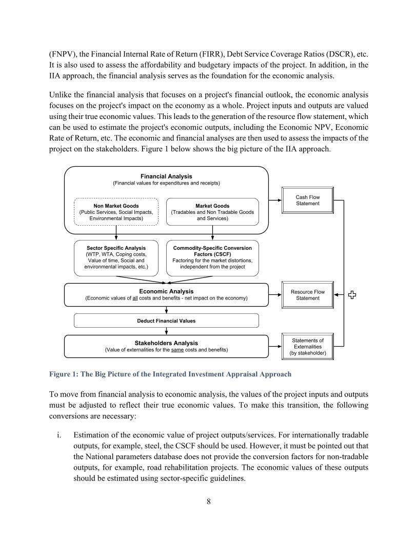
Unlike the financial analysis that focuses on a project's financial outlook, the economic analysis focuses on the project's impact on the economy as a whole. Project inputs and outputs are valued using their true economic values. This leads to the generation of the resource flow statement, which can be used to estimate the project's economic outputs, including the Economic NPV, Economic Rate of Return, etc. The economic and financial analyses are then used to assess the impacts of the project on the stakeholders. Figure 1 below shows the big picture of the IIA approach.
Figure 1: The Big Picture of the Integrated Investment Appraisal Approach
To move from financial analysis to economic analysis, the values of the project inputs and outputs must be adjusted to reflect their true economic values. To make this transition, the following conversions are necessary:
i. Estimation of the economic value of project outputs/services. For internationally tradable outputs, for example, steel, the CSCF should be used. However, it must be pointed out that the National parameters database does not provide the conversion factors for non-tradable outputs, for example, road rehabilitation projects. The economic values of these outputs should be estimated using sector-specific guidelines.
Financial Analysis(Financial values for expenditures and receipts)
Non Market Goods(Public Services, Social Impacts,
Environmental Impacts)
Market Goods(Tradables and Non Tradable Goods
and Services)
Economic Analysis(Economic values of all costs and benefits - net impact on the economy)
Sector Specific Analysis(WTP, WTA, Coping costs, Value of time, Social and
environmental impacts, etc.)
Commodity-Specific Conversion Factors (CSCF)
Factoring for the market distortions, independent from the project
Deduct Financial Values
Stakeholders Analysis(Value of externalities for the same costs and benefits)
Cash Flow Statement
Resource Flow Statement
Statements of Externalities
(by stakeholder)
9
ii. Estimation of the economic resource costs of project inputs. This involves the application of the CSCFs to convert the market values of the project inputs to their economic values. The inputs are generally divided into three categories:
a. Tradable project inputs; b. Non-tradable project inputs; and c. Labour
iii. Substitution of the discount rate used in the financial analysis (sometimes the ROE) with the economic opportunity cost of capital (EOCK)
Illustration
Box 1: Project Introduction
As part of its mandate to contribute to the National Development Plan of eliminating poverty
and reducing inequality by 2030, the Ministry of Agriculture has identified that investing
specifically in the cultivation of maize will play a significant role in achieving this objective.
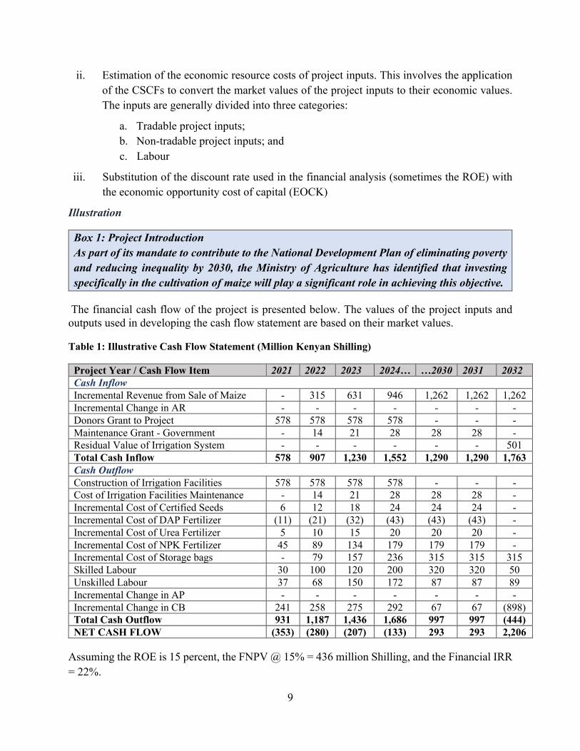
The financial cash flow of the project is presented below. The values of the project inputs and outputs used in developing the cash flow statement are based on their market values.
Table 1: Illustrative Cash Flow Statement (Million Kenyan Shilling)
Project Year / Cash Flow Item 2021 2022 2023 2024… …2030 2031 2032 Cash Inflow Incremental Revenue from Sale of Maize - 315 631 946 1,262 1,262 1,262 Incremental Change in AR - - - - - - - Donors Grant to Project 578 578 578 578 - - - Maintenance Grant - Government - 14 21 28 28 28 - Residual Value of Irrigation System - - - - - - 501 Total Cash Inflow 578 907 1,230 1,552 1,290 1,290 1,763 Cash Outflow Construction of Irrigation Facilities 578 578 578 578 - - - Cost of Irrigation Facilities Maintenance - 14 21 28 28 28 - Incremental Cost of Certified Seeds 6 12 18 24 24 24 - Incremental Cost of DAP Fertilizer (11) (21) (32) (43) (43) (43) - Incremental Cost of Urea Fertilizer 5 10 15 20 20 20 - Incremental Cost of NPK Fertilizer 45 89 134 179 179 179 - Incremental Cost of Storage bags - 79 157 236 315 315 315 Skilled Labour 30 100 120 200 320 320 50 Unskilled Labour 37 68 150 172 87 87 89 Incremental Change in AP - - - - - - - Incremental Change in CB 241 258 275 292 67 67 (898) Total Cash Outflow 931 1,187 1,436 1,686 997 997 (444) NET CASH FLOW (353) (280) (207) (133) 293 293 2,206
Assuming the ROE is 15 percent, the FNPV @ 15% = 436 million Shilling, and the Financial IRR = 22%.

10
To convert the items in the cash flow statement to their corresponding economic values (resource cost and benefits), the CSCF of each item is obtained using the National parameters database, following the steps discussed above.
i. Estimate the economic value of the output: The output of this project is maize (corn). Since maize is one of the agricultural produces that Kenya exports, the project produces an exportable output. On the National parameters database, we select the “Tradables” tab, and we can either search by “Commodities” or by “Categories.” If we choose “Commodities,” we can then type the project output into the search bar. This might bring up several related commodities, out of which the most applicable is selected. In this case, we choose “Maize (corn) flour,” and we specify that it is an exportable output. This gives a conversion factor of 1.0500. To obtain the economic value of the project output (maize), we multiply the market value by the conversion factor. It is worth noting that when the CSCF of a commodity is greater than 1, it means that the economic value of the commodity is greater than its market value.
ii. Estimate the resource costs of inputs: This involves the application of the CSCFs to convert all the cost items of the project to their corresponding economic value. This is achieved by multiplying the market values by the corresponding CSCF.
a. Tradable project inputs: An example of an input that falls under this category (in the illustrative example) is the DAP fertilizer, an importable input. Following similar steps to those described in i above, the National parameters database is used to obtain the CSCF of 0.9953. The market value of DAP is then multiplied by 0.9953 to get the economic cost of DAP fertilizer. If the CSCF of an input is less than 1, it means that the economic cost of the commodity is less than its financial cost.
b. Non-tradable project inputs: An example of such input is the construction of irrigation facilities. To obtain the CSCF for this project input, the “Non-tradables” tab is selected, and “construction” is picked as the commodity of interest. Doing this gives a CSCF of 0. 0.8140. Again, the economic value is obtained by estimating the product of the market value of construction and a CSCF of 0. 0.8140.
c. Labour: The concept of EOCL is premised on the fact that employing a person (a resource) for one project implies that the individual is giving up other opportunities that would utilize their time. In other words, people are being drawn away from their other productive activities. However, when a project pays a wage higher than a person's alternative wage elsewhere, it creates a positive externality (benefit to the employee). Similarly, in this situation, the project will also generate a positive fiscal externality. The higher wage rate will put the worker in a higher tax bracket, thus increasing the tax paid/generated by the employee. All of these are accounted for in the estimation of the conversion factors for all categories of Labor in Kenya.
11
The National Parameters Database takes account of the different categories of workers in Kenya. Similar to the non-tradables, the CSCF for labour is obtained by selecting the “Labour” tab and picking the category of interest. The CSCF for skilled labour is 0.80.
iii. Substitution of the discount rate with the EOCK. The EOCK is a national parameter and is not project-specific, and it represents the opportunity cost of investing resources into the project from the perspective of the economy. Instead of the ROE or the discount rate used in the financial analysis, the EOCK is used to discount the project’s net resource flow. To obtain the EOCK using the National parameters database, the “National Parameters” tab, which contains all the estimated national parameters, is selected. The EOCK for Kenya was estimated to be 11.5%.
The economic resource flow statement of the illustrative project is presented below. To obtain the economic values of the project inputs and outputs presented in the resource flow statement, each of the items in the cash flow statement is multiplied by their corresponding CSCFs.
Table 2: Resource Flow Statement (Million Kenyan Shilling)
CF 2021 2022 2023 2024… …2030 2031 2032 Resource Inflow
Incremental Revenue from Sale of Maize 1.05 - 331.2 662.3 993.5 1,324.7 1,324.7 1,324.7
Incremental Change in AR 1.00 - - - - - - - Donors Grant to Project 0 - - - - - - - Maintenance Grant - Government 0 - - - - - - -
Residual Value of Irrigation System 0.81 - - - - - - 407.89
Total Resource Inflow - 331.2 662.3 993.5 1,324.7 1,324.7 1,732.5 Resource Cost Construction of Irrigation Facilities 0.81 470.49 470.49 470.49 470.49 - - -
Cost of Irrigation Facilities Maintenance 0.99 - 13.99 20.99 27.98 27.98 27.98 -
Incremental Cost of Certified Seeds 0.80 4.83 9.66 14.48 19.31 19.31 19.31 0.00
Incremental Cost of DAP Fertilizer 0.99 (10.67) (21.35) (32.02) (42.70) (42.70) (42.70) 0.00
Incremental Cost of Urea Fertilizer 0.99 5.05 10.10 15.15 20.20 20.20 20.20 0.00
Incremental Cost of NPK Fertilizer 0.99 44.42 88.83 133.25 177.66 177.66 177.66 0.00
Incremental Cost of Storage bags 0.70 0.00 54.88 109.76 164.64 219.52 219.52 219.52
Skilled Labour 0.80 24.00 80.00 96.00 160.00 256.00 256.00 40.00 Unskilled Labour 0.89 32.77 60.95 133.62 152.89 77.09 77.09 79.49 Incremental Change in AP 1.00 - - - - - - -

12
Incremental Change in CB 1.00 241.27 258.10 274.94 291.77 67.33 67.33 (897.75) Total Resource Cost 812.16 1025.65 1236.65 1442.25 822.40 822.40 (558.74) NET RESOURCE FLOW (812.16) (694.49) (574.33) (448.76) 502.25 502.25 2291.28
ENPV @ EOCK (11.5%) = 151.31 million Shilling, ERR = 13%
It should be pointed out that a conversion factor of zero implies that the item is a transfer. Items such as taxes, subsidies, grants, etc., are treated as transfers (moving money from one pocket to another) in the economy. Therefore, they are not added to or deducted from the economic resource flow statement.
4. The Role of National Parameters in Public Planning and Appraisal
Unlike the CSCFs, which are specific to commodities and depend on the inputs used up and the outputs produced by the project, national parameters are country specific. These parameters are to be used for all projects in Kenya. They include the economic opportunity cost of capital, foreign exchange premium, and non-tradable outlay (NTP). The following sections discuss each estimated parameter and how they are used to plan and appraise public investment projects.
4.1. Economic Opportunity Cost of Capital
Public investment projects usually last for many years; therefore, the planning and appraisal of such projects require a comparison of the benefits generated by the project and the costs incurred by the project over its entire lifetime. To estimate the PV of project resource costs and benefits, the EOCK is used to discount the project’s net resource flow. The term “discount rate” rate, in this case, refers to the time value of the costs and benefits from the viewpoint of the society. For example, suppose the NPV of a project is greater than zero, i.e., the benefits outweigh the resource costs. It implies that the project would generate more net economic benefits than the same resources would have generated if used elsewhere in the economy.
It must be stated that the choice of the discount rate used to estimate the PV of resource costs and benefits is an important decision. This is because different choices can result in entirely different outcomes and, consequently, the decision on whether the project should proceed to the next stage or otherwise. For example, suppose instead of the estimated EOCK of 11.5%, a discount rate of 13% is used to estimate the project economic NPV of the illustrative project. In that case, the project becomes economically unviable with a negative NPV of (50.77) million Shilling. On the other hand, if the discount rate is 10%, the project generates a much higher NPV of 384.85 million Shilling. Therefore, it is important that the same discount rate (EOCK) is used for economic analysis throughout Kenya.
For Kenya, the economic opportunity cost of capital was estimated to be 11.5 percent. This value is recommended to be used in the economic appraisal of all infrastructure projects in Kenya. Details of the methodology utilized in the estimation are presented in Annex A.

13
4.2. Foreign Exchange Premium and Premium for Non-Tradable Outlays
The other national parameters used to appraise investment projects are Foreign Exchange Premium FEP and the Premium for Non-Tradable Outlays (NTP). These premiums are generated because of trade and other indirect tax and subsidy distortions at the point in time that the funds are raised in the capital market and spent on tradable and non-tradable goods. To effortlessly incorporate FEP and NTP in the economic evaluation of projects, FEP and NTP are expressed as a percentage of the market foreign exchange rate and financial value of non-tradable goods, respectively.
In practice, these parameters are used as inputs in estimating the CSCFs for tradable and non-tradable inputs. They represent some of the distortions that are accounted for when the conversion factors of commodities are estimated. For example, the distortions observed in the market value of urea fertiliser (from the illustrative example) are the FEP and the VAT. Adjusting for these distortions results in a commodity-specific conversion factor of 0.9953.
A change in the value of these national parameters will lead to a different result of the CSCF estimates. The FEP for Kenya was estimated to be 5 percent, and the NTP is 1.0 percent. Details of the methodology used to estimate the FEP and NTP are presented in Annex A.
5. Conclusion
The National Parameters Database is a web-based Kenya CSCF database software. This web-based software provides open access to the national parameters and CSCFs for tradable and non-tradable commodities and services. The program provides multiple ways to search and browse the database with a user-friendly interface. It is designed for professionals, policymakers, and academia involved in the economic and social appraisal of public investment projects in Kenya.
Moving from financial analysis to economic analysis is a crucial component of public investment project planning and appraisal. Project Sponsors are expected to accurately demonstrate that the project is economically viable before the project is considered for implementation. The transition to economic analysis involves the estimation of conversion factors used to covert the market values of project input and output to their corresponding economic values. This estimation is technical, tedious, and time-consuming. Therefore, the National parameters database plays a significant role in enhancing the ease with which Project Sponsors conduct economic analysis. The National parameters database provides a compilation of the conversion factors and national parameters that can be directly applied when conducting the economic analysis of projects.
Not only does the National parameters database improve the ease of conducting economic analysis, but it also helps to maintain the integrity of the economic analysis by enhancing its accuracy. For example, the choice of discount rate can significantly impact the economic outlook (in terms of viability) of the project, as a result, impacting the decision-making process. The conversion factor

14
and national parameters estimates contained in the National parameters database were estimated with a high level of attention, accuracy, and appropriate methodologies were employed.
However, it is worth noting that the National parameters database does not provide the CSCFs for non-tradable outputs, such as roads, water and sanitation, etc. The economic values of such outputs should be estimated individually, using sector-specific guidelines. For example, the benefits of a road project generally arise from the value of time saved due to the project, vehicle operating cost savings, reduction in the number of accidents, etc.
5.1. Recommendations
To reap all the benefits of the National parameters database, attention should be given to the following recommendations:
1. The National parameters database usage should be mandatory for every organ of state involved in public planning and appraisal when conducting the economic analysis of projects. This will ensure that the same parameters are used throughout the country and improve the accuracy of comparing the viability of projects.
2. Detailed cost estimates should be obtained from engineering studies. Different commodities serve as inputs of the project, and each of these commodities has specific conversion factors. For example, instead of obtaining the total capital expenditure of a project from the engineering studies, the Project Sponsor should disaggregate the components of the capital expenditure as much as possible. This will ensure that CSCFs are applied to all the different elements that constitute the capital expenditure and enhance the accuracy with which they are converted from their market values to their corresponding economic values.
3. To complement the National parameters database, it is important that sector-specific guidelines be developed. In addition, government officials should undertake capacity-building programs on how to conduct investment appraisals using the IIA approach and how to use the National parameters database.

[This page was intentionally left blank]

Annexure A: Kenya National Parameters Report

Estimation of the National Parameters for Project Evaluation in Kenya Final Report
Submitted by: Cambridge Resources International, Inc. 1770Mass.Ave#617,Cambridge,MA02140,USA Phone: 1 (613) 770 2080 E-mail: [email protected] or [email protected]
In Consortium with: GEEKAN KENYA LTD RUPRANI HOUSE, MOKTAR DADAH P.O BOX 17460-00100 TEL:+254723729096 Email: [email protected] NAIROBI-KENYA. Presented to: THE MINISTRY OF NATIONAL TREASURY AND PLANNING, KENYA

18
Executive Summary
In this paper, an analytical framework and a practical approach are developed to measure
the economic opportunity cost of capital (EOCK) and the foreign exchange premium
(FEP), and the premium for non-tradable outlays (NTP). These national parameters are the
essential determinants for practical application to the economic appraisal of investment
projects in a consistent manner for a country.
An application of the model is carried out for Kenya since Kenya is a small open economy
and is also well integrated into the global capital market. Estimate of the EOCK is based
on the hypothesis that when funds are raised in the capital market to finance any investment
project, those funds are likely to come from displaced investment, newly stimulated
domestic savings, and newly stimulated foreign capital inflows. It can then be estimated as
a weighted average of the opportunity cost of each of the three alternative sources of funds.
The EOCK is the most appropriate rate used to discount the economic benefits and costs
of a project to see if the project is economically viable for society as a whole.
The empirical results generate 11.36% of the EOCK for Kenya in the base case. To ensure
the robustness of the estimates, a sensitivity analysis is conducted for the key parameters
used in the study. The simulation results range from 9.91% to 12.7% and center around
11.4%. Given the data obtained and used for the analysis, these results suggest that an 11.5
percent real rate is an appropriate and conservative discount rate to use when calculating
the net present value of the flows of annual economic benefits and costs over the life of a
project.
The foreign exchange premium (FEP) reflects the difference between the economic value
of foreign exchange and the market exchange rate owing to the existence of indirect taxes
and production subsidies involved in both domestic and external transactions. Likewise, a
premium for non-tradable outlays (NTP) is generated because of the set of taxes and
subsidies that cause the shadow price of non-tradable goods to be greater or less than their
financial values. These premia are quantified and used to convert the financial values of

19
tradable and non-tradable inputs and outputs into their corresponding economic values for
a project’s implementation and operation.
The framework for measuring these premiums is based on a three-sector general
equilibrium model in an economy, including importable, exportable, and non-tradable
goods in which the first two are combined as tradables. The model is further developed
into an operational simulation model to capture the distortions associated with changes in
demand and supply between the tradable and non-tradable sectors after funds are raised in
the capital market and spent on tradable goods and non-tradable outlays.
The model is carried out to estimate the FEP and the NTP for Kenya. In the base case, they
are estimated at 5.29% and 0.84%, respectively. A sensitivity analysis is also conducted
for the key parameters. The simulation results indicate that the FEP ranges from 4.77% to
5.58%, while the NTP from 0.30% to 1.81%. These results suggest that the reasonable
values of the FEP and the NTP for Kenya will be 5.2 percent and 1.00 percent, respectively.

20
1 Introduction
This study is developed to provide an analytical framework to government organizations
and their personnel involved in public investment management with the aim to facilitate
the empirical measurement of two national parameters required for the completion of an
accurate and consistent economic appraisal or cost-benefit analysis of investment projects
in Kenya. These parameters are the economic opportunity cost of capital (EOCK) and the
foreign exchange premium (FEP), and the premium for non-tradable outlays (NTP).
The economic opportunity cost of capital (EOCK) is a discount rate used to compare
benefits and costs that occur at different times of an investment project to see whether the
proposed public project or policy is feasible from the economy’s point of view. If, on the
one hand, the economic NPV of a project is positive, it is potentially worthwhile to
implement the project. This implies that the project increases efficiency or raises the wealth
of the country as it produces enough benefits to fully compensate all individuals in the
economy. On the other hand, if the NPV is less than zero, the project should be rejected on
the grounds that the resources invested would have yielded a higher economic return if
they had been left for the capital market to allocate to other uses. The economic discount
rate is similar to the concept of the private opportunity cost of capital used to discount the
financial cash flows of an investment to find its financial net present value. However, the
deviations of financial values from economic values of project costs and benefits may arise
from various market distortions that are often created by government interventions such as
taxes, subsidies, and price controls or by imperfect competition.
The FEP is needed to convert the financial values of foreign exchange content into its
corresponding economic values in order to measure the economic value of tradable goods
and services purchased or produced by the project. With the existence of various distortions
such as import tariffs, export taxes, production subsidies, and other indirect commodity
taxes, the market exchange rate does not accurately reflect the economic value of a unit of
foreign exchange in relation to domestic currency. It is this economic (shadow) exchange
21
rate that should be used to convert the values of tradable goods. This adjustment will ensure
that the project’s use or generation of foreign exchange adequately reflects the economic
opportunity cost of foreign exchange in the country. Likewise, these distortions create a
gap between the economic cost of the resources used to purchase non-tradable goods and
services employed by a project and their financial values.
Estimates of these parameters depend on Kenya’s economic structure and the types and
sizes of the taxes and subsidies in its markets. Regarding the employment structure, while
the share of the labor force engaged in agriculture is generally declining over the past ten
years, agriculture still remains the largest employer of labor, accounting for 54.34% of total
employment.3 In terms of sectoral composition, services remained the dominant sector,
accounting for 42.19% of the total value of the economy in 2020. Agriculture has been
growing over the last decade and standing now at 35.15% of GDP.4
Following the 2014 rebasing of its economy, Kenya is now classified as a lower-middle-
income country. In 2019, Kenya’s economy was considered the largest economy in East
Africa and Central Africa and the third biggest in sub-Saharan Africa (SSA).
The expected economic growth and development path for Kenya is outlined in Vision
2030, a long-term development blueprint for the country. The vision aims to transform
Kenya into a newly industrializing, middle-income country that provides a high quality of
life to all its citizens in a clean and secure environment.
The economic pillar of the Vision 2030 targets sustained 10 percent annual average GDP
growth until 2030, beginning 2012. Although the highest economic growth rate achieved
has been so far 8.4 percent during the year 2010, the average growth rate over the period
3 See, International Labour Organization, ILOSTAT database. 4 See, The World Bank, World Development Indicators.

22
2012-2019 has been far below the targeted growth rate with 5.49 percent realized economic
growth.5
To achieve the desired economic growth, Kenya Vision 2030 and the “Big Four” agenda
underscore the need for massive investment and infrastructure projects, including roads,
housing, power projects, and health facilities. These investments are projected to be
primarily financed by gross national savings. However, the savings level of the country has
remained low, maintaining a persistently significant savings-investment gap. 6
Furthermore, Kenya’s government budget has been in deficit over the past decade and a
half. Borrowing has been a key resource in financing the budget. Accordingly, Kenya’s
public debt has been increasing over time and reached the Ksh 5.0 trillion mark in June
2018 and Ksh 5.8 trillion in June 2019, reflecting the government’s growing appetite to
borrow to fund infrastructure projects across the country.7
According to Vision 2030, Kenya needs to boost its total investments to at least 30 percent
of GDP. However, the national accounts data show that investment rates fall short of the
set targets. For instance, during the first Medium-Term Plan MTP(I), total investments
were 20.4 percent of GDP, compared to a target of 25.0 percent, whereas it was 20.1
percent in the second Medium Term Plan MTP (II) against the target of 28.0 percent. The
overall investment levels have not sparked the expected economic development, with some
major projects listed in Vision 2030 still awaiting completion.8
Despite the fact that infrastructure investment makes a significant contribution to national
economic growth (Aschauer,1989), the level of investment (quantity) would not translate
5 Economic growth rates have stagnated at 5.37% in 2019, 6.32% in 2018, 4.81% in 2017, 5.88% in 2016, 5.72% in 2015, and 5.36%, 5.88%, and 4.56% in 2014, 2013 and 2012, respectively. See, The World Bank, World Development Indicators 6 According to Kenya Economic Report , 2020, the savings-investment gap ranging from 5.3 per cent to 12.1 per cent of GDP for the period 2012 to 2017 but recorded 7.1 per cent in 2018. The savings-investment gap widened to 8.3 per cent of GDP in 2019. These levels of gross national savings are not enough to adequately finance the required investment levels, and hampering and delaying the realization of Kenya’s development goals. 7 See, Kenya Economic Report, 2019. 8 For the sake of comparison,it is worth mentioning that in 2015 The share of gross fixed capital formation (GFCF) in GDP reached to 34.25% in Tanzania at 2015, and 27.94% in Uganda at 2013.

23
into faster economic growth rates or a longer-lasting growth effect if the capital
productivity (quality) of the investment does not improve. With the existence of a
crowding-out effect induced by public demand for funds on private investment, the
selection of public investments yielding social returns lower than the opportunity costs of
funds is economically non-viable. It can reduce output and productivity growth as the
resources they employ would have made a higher benefit elsewhere in the economy.
Scaling up the public capital stock in infrastructure, according to Agénor & Moreno (2006),
may have a negative impact on growth in the short and medium terms if it crowds out
private investment. This short-term impact might be converted into an unfavorable
economic effect if the drop in private capital investment sustains over time.
These challenges necessitate enhanced domestic resource mobilization, increasing the
importance of the direction of the country's resource allocation and the efficiency of the
provision of public infrastructure. Public investments need to be made in a structured,
considered manner to prevent inappropriate initiatives, protect Kenya's resources, and
ensure that prioritized investments are efficiently implemented. Poor investment decisions
commandeer the economy's resources and hinder other important investments, ultimately
constraining economic growth.
Governments often have many investment opportunities, and a highly relevant issue is
which of these investment opportunities should be adopted. A consensus is that a project's
present value is the correct measure of the project's contribution to social welfare. In fact,
the present value criterion suggests that any (independent) project can only be adopted if
its present value is positive. A key piece of information inside the present value criterion
is the discount rate that is used to aggregate benefits and costs over time. In economic
project evaluation, we need a discount rate that accounts for existing distortions in capital
markets. In other words, we need a social discount rate or, equivalently, a rate of discount
capturing the economic opportunity cost of capital. Applying this discount rate in Kenya
public projects' economic analysis would help improve investment allocations and project
selection processes to ensure that the best investment projects are selected and funded.

24
Given the limited investment resources available to implement high levels of investment
across various sectors, the purpose of discounting in the appraisal of public projects is to
choose the rate that best promotes economic efficiency in terms of maximizing net present
values of public benefits, such that this rate leads to a selection of more productive project
over another that is less productive. This enables the government to cut out inferior projects
and invest in those with a potential high yield to meet the Vision 2030 targets and provide
the best benefits for the current and future generations.
Improving the growth effect and minimizing the inefficiencies in the government's use of
capital requires that any public investment is expected to yield a higher return in social
terms than what would be earned by the economy if the funds were left in the capital
market. Accordingly, the economic return from the investment in any project must
compensate for the weighted economic cost of the sources of the funds used to finance it.
This includes the (1) displaced domestic investment, (2) incremental forgone consumption,
and (3) in an open economy, paying for the incremental funding sourced from abroad.
Furthermore, the opportunity cost of capital also has an essential role in the choice of
technology for a project during the project design process. “The use of a lower financial
cost of capital instead of its economic opportunity cost would create an incentive to use
production techniques that are too capital intensive. The choice of an excessively capital-
intensive technology would lead to economic inefficiency because the value of the
marginal product of capital in this activity is below the economic cost of capital to the
country”. (Jenkins et al., 2019).
2 Measurement of the Economic Opportunity Cost of Capital (EOCK)
2.1 Alternative Approaches
Implementation of cost-benefit analysis involves the important step of choosing an
economic discount rate. Economists are in agreement that a very serious misallocation of

25
resources can result from the use of an incorrect estimate of the economic discount rate.9
While methods of estimating market discount rates are well known, the appropriate method
of selecting an economic discount rate to be used in evaluating public sector investment
projects has been one of the most contentious and controversial issues in this area of
economics.
Based on efficiency criteria, methods for determining the economic discount rate are
generally placed into three categories.10 The first one is the evaluation of consumption that
is related to the ‘social rate of time preference’ approach about society's willingness to give
up an amount of consumption today in exchange for more in the future but only after
adjusting the costs by the ‘shadow price of capital’ to take into account the existence of a
higher marginal productivity rate of return on the displaced investments.
The second viewpoint of growth maximization focuses on the highest rate of return of an
investment available outside of the public sector that could be financed by these funds. It
has usually been the case that this option is to finance investment projects in the private
sector.
The third method captures the essential features of the above two alternatives by taking
into account the social opportunity cost of public investment as well as the impact of public
investment on consumption spending, considering the capital market is the marginal source
of funds. This method is founded on the contributions of Harberger. It recommends the use
of a weighted average of the ‘marginal productivity of capital’ in the private sector, the
‘rate of time preference for consumption,’ and the ‘marginal cost of foreign financing,’
with the value of weights representing the fractions of funds diverted from displaced
investment demand, forgone consumption (increase in domestic supply of savings) and
9 See, for e.g., Baumol (1968); Harberger (1969); Burgess (1988). 10 Social rate of time preference as supported by: (Marglin, 1963), (Feldstein, 1964), (Sen, 1961), (Lind, 1982), (Bradford, 1975). Social opportunity cost of capital advocates by: (Baumol, 1968), (Mishan, 1967), (Diamond, P. & J. Mirrlees.,1971). The Weighted average approach as supported by: (Harberger, 1969), (Usher, 1969), Ramsey (1969), (Sandmo & Drèze, 1971), (Sjaastad & Wisecarver, 1977), (Harberger & Wisecarver, 1977), Boadway (1978), Hagen (1983), Marchand and Pestieau (1984), (Burgess D, 1988), (Jenkins, Kuo, & Harberger, 2019), (Burgess & Zerbe, 2013), and (Harberger & Jenkins, 2015).

26
foreign savings when the government enters into a borrowing operation in the capital
market.
In this study, we apply this weighted average approach using Kenya national accounts and
capital market information in order to estimate the appropriate economic discount rates to
be used for appraising public investment projects in Kenya.11 What follows is to describe
this approach and empirically measure the economic cost of capital for Kenya.
2.2 Analytical Framework
The estimation of the (EOCK) is based on the view that “the ‘marginal’ source of funds for
both the public and private sectors is usually the capital market (Jenkins & Kuo, 1998).
When the sponsor of an investment project enters the capital market and bids for funds, the
private demand for funds as well as the domestic supplies of investible funds are likely to
respond to a change in market conditions. An increase in the cost of funds causes a
postponement of some private investment in the country. On the other hand, domestic
consumers tend to postpone their current consumption in order to save more as they are
attracted to a greater amount of consumption that they can spend in the future by now
saving and investing their funds in the capital market.
When we move to an open economy framework, borrowing from the international capital
market becomes the third source of funds due to a higher rate of return in the home country.
According to Sandmo & Drèze (1971) and Edwards (1986), the supply of funds from
foreign savers depends positively on the rate of interest; hence, more foreign savers are
attracted to the country's capital market. In this case, the cost is not solely the cost of
servicing the incremental foreign loans but also the additional costs of servicing the
existing foreign debt where the interest rate on some of the current stock of debt is
contracted at a variable interest rate. These debt instruments would be responsive to
changes in the market rate of the interest.
11 This approach has been initially developed by Harberger (1969) and Sandmo & Dreeze (1971).

27
In sum, the EOCK is a weighted average of the economic cost of funds from the three
sources employed to finance the additional demand marginal investment project, with
weights reflecting shares of funds extracted from their respective sources. They should be
measured by the responsiveness of investors and savers to changes in interest rates caused
by the government's additional demand for funds. This can be expressed as:
EOCK = f1*r + f2*r + f3*MCf (1)
Where ρ refers to the gross tax rate of return to domestic reproducible remunerative capital
investment, r stands for the economic cost of newly stimulated household savings, and MCf
for the marginal economic cost of foreign financing. The corresponding weights (ƒi)
represent the share of funds diverted from private sector investors, private sector savers,
and foreign savers. The sum of ƒ1 + ƒ2 + ƒ3 will equal one.
2.3 Empirical Estimation
Following equation (1), estimating the economic opportunity cost of capital requires the
estimation of two components. The first component is presented in section 2.3.1 and is
concerned with the estimation of the economic cost of each of the three sources of
investment funds, namely, the economic rate of return on displaced reproducible
remunerative investments, the rate of return of on domestic savings (net of tax), and the
marginal economic cost of foreign financing. Section 2.3.2 presents the estimation of
shares of these three sources of funds.
2.3.1 The Economic Opportunity Cost of the Different Sources of Public Project Funds
2.3.1.1 The Gross of Tax Rate of Return on Reproducible Remunerative Capital (ρ)
The gross-of-tax return to reproducible remunerative capital measures the contribution of
remunerative capital investment in the economy as a whole. In most estimates of the
economic discount rate based on the weighted opportunity cost of funds, the largest share
of the opportunity cost comes from the reduction in domestic reproducible remunerative
28
capital investments. The relevant opportunity of funds will be partially determined by the
economic return of those investments that will be displaced by the government’s capital
market operations.
The measurement of the return to capital can be reached by two main alternative
approaches; while the two approaches are using the national accounting system, however,
they are different in the way of calculating the flow of income generated by capital. The
first method has been applied to Canada by Jenkins & Kuo (2007). In this method, the
income to capital in the country is estimating by adding up all the returns to capital which
includes interest income, dividend income, rent, profit income, as well as the associated
direct and indirect taxes generated by capital. The total income accruing to capital is then
divided by the stock of reproducible remunerative capital. The second approach is an
aggregate and top-down approach.12 At a conceptual level, if we assume that factor
payments exhaust the value of output, we can obtain income accruing to capital as the value
of output net of the contributions made by labor, land, natural resources, associated sales,
and excise taxes and the gross consumption of fixed capital. According to the availability
and types of detailed data recorded in Kenya’s national accounts, the second approach is
adopted.
The rate of return to reproducible remunerative capital (!) at time t is the ratio of the value
of national income (net of economic depreciation) that has accrued to capital ("!") to the
value of the reproducible remunerative capital stock (#!). with both numerator and
denominator expressed in terms of prices of the same year
! = #!""!
(2)
12 The approach was first applied by Harberger & Wisecarver (1977) to calculate the rate of return to capital for Uruguay. This method was applied by Poterba (1998) to measure the ‘rate of return to corporate capital’ in United States, and used by Jenkins & Kuo (1998), Kuo et al. (2003) and Coppola et al (2014) to estimate the rate of return on capital as one of components used in calculating the economic discount rate for Philippines, South Africa and Mexico, respectively.

29
In accordance with Gollin (2002), macroeconomists commonly calculate the shares of
production factor not from data at the firm level but from national income accounts data
and product accounts. The most used method in order to estimate the share of capital in
GDP at current market prices is to estimate the labor share of national income from the
share of employee compensation in GDP. The returns to capital are then taken to be
residual” and can be expressed as follows:
"!" ="! −"!$ (3)
Where "! represents the national income and "!$ is the total labor income. Moreover, we
will need to find the value of GDP after subtracting the contributions related to land and
natural resources, associated indirect taxes, and the depreciation expense. Therefore, our
proposed capital income at time t is specified as follows:
"!" ="! −"!$ − '()*!% −+$,! − -! − .! (4)
Where in a given year t, "!" is the return to capital, "! is the national income, "!$ is the total
labor income, ()*!% is the gross value added of agriculture, ' is the proportion of land's
contribution to ()*!%,+$is Labor's share of national income, ,! represents the sales and
excise taxes, +$,! is the amount of taxes on products borne by the value-added of labor,
-! is the value of natural resource rents, and .! is the depreciation expense associated with
the reproducible capital stock.
The first step is to estimate the total labor's share of national income representing the sum
of wages and salaries paid to the workers by corporations plus the labor income of the non-
incorporated enterprises. Since the owners or the members of unincorporated enterprises
are working without receiving wages and salaries, this sector's operating surplus includes
income accruing to both labor and capital. Therefore, the faction of mixed-income that
corresponds to the labor income for unincorporated enterprises needs to be estimated and
added to the total remuneration paid to employees in the national accounts in order to find
out the total income accruing to labor created by the economy in a given year.
30
The compensation of employees, which represents the lower bound of total labor income
in the economy, is available in the national accounts of Kenya; however, this item generally
disregards the self-employed income, and without considering this share, the labor income
will underestimate the true total labor income share. Therefore, to estimate the total share
of labor in national income, one needs to add up the share of labor income of
unincorporated businesses to the compensation of employees’ items of national accounts.
To determine the total labor income in Kenya, we employ the ILO modelled estimates
(2019) of the labor income share in GDP. The ILO estimate provides the ratio of total labor
income (after accounting for the labor income of the self-employed) and gross domestic
product (a measure of total output), both provided in nominal terms.13
According to the data obtained from the ILO dataset, the total share of labor in GDP for
Keny ranges between 41.5% to 46% of national income between 2006 to 2019. In the
empirical estimations that follow, sensitivity analysis is run to define the effect of changes
in the labor income share and on the estimation of EOCK.14
The second step is to figure out income accruing to land. As land is not part of reproducible
capital, it is not part of the base of our rate of return estimation. This task is not
straightforward because we do not have direct information on the income generated by
land; however, the land is a production factor contributing significantly to the value-added
in the agriculture and housing sectors.15
Agriculture is a large sector in Kenya which accounting for about a third of the total value
of the economy.16 According to Harberger (1969) and Robles (1997), one-third of the
13 Self-employed can be found in the revision of the International Classification of Status in Employment, ILO (1993), and includes – among others – employers, own-account workers and contributing family workers. Employers are self-employed individuals who engage at least one employee on a regular basis. In contrast, own-account workers do not engage employees on a regular basis. Finally, contributing family workers work in an establishment operated by a relative with a limited degree of involvement in its operation. 14 All data are presented for the total share of labor income is shown in Appendix A. 15 Disaggregated items of the GVA of housing sector or on the contribution of land to the sector are not available for Kenya. Accordingly, in the absence of detailed information, the housing sector is excluded from this study. 16 Agriculture, forestry and fishing accounting for 34% of the gross domestic product in 2019.
31
value-added in the agricultural sector is an income accruing to land.17 Kenya national data
indicates that the gross value added by agriculture in the aggregate sector ranges between
91.56% to 95.17%.18 Hence, we estimate the land contributions in the agriculture sector to
the GDP as (1/3), multiplying by the sum of gross value added of growing of crops and
animal production sub-sectors as shown in Appendix A, column (8).
The third component to be deducted from the income to capital is natural resource rents, as
it is not a return to reproducible capital. Natural resources combined with reproducible
capital give rise to economic rents.
The mining and quarrying sector makes a negligible contribution to the Kenyan economy.
The national figures show that the average rate of mining and quarrying output to GDP
over 2006 - 2019 is less than one percent.
From 2016 to 2019, the total royalty and natural resource income received by the
government from the mining sector fall in a range between 3.1% to 5% of the gross value
added of the industry.19 In the absence of more precise data, we assume that the value of
economic rents in Kenya that need to be deducted from the national income is only the
share of total royalties in the mining sector. However, we expect this estimate to be
somewhat underestimated of the share natural resources as the income received from the
free mining equity and the corporate tax on economic rents received by the government are
not accounted for in this study.20
The fourth part is indirect taxes and subsidies. Indirect taxes mainly include sales tax (i.e.,
value-added tax charged on the sale of goods or services), excise tax, and customs duties
that are all included in GDP at market prices. To account for the return to reproducible
17 Fishing and forestry are excluded. 18 The data is obtained from KNBS, national accounts for 2006 to 2019. 19 The prevailing royalty rates in Kenya are: Gold, fluospar, diatomite, CO, (5%), Mettalic ores (8%),Titanium (10%), Gemstones (5%), Industrial minerals (1%), and Cement mineral levy 140/= per tonne. Those rates are available at, https://www.petroleumandmining.go.ke/state-department-for-mining. 20 We assume that the total economic rents of Kenya that need to be deducted from the national income would be 3.5 percent of the gross value added of mining and quarrying sector as presented in Column (9) in Appendix A.

32
capital, we need to allocate the total amount of indirect taxes between the value-added of
capital and the value-added of labor.
Regarding sales taxes, Kenya has implemented a value-added tax (VAT) at a rate of 16%
currently. These value-added taxes apply to the consumption of goods and services in the
economy. VAT is charged at each stage of the production and distribution process, and it
is proportional to the price charged for the goods and services. Kenya's government allows
the vendors full credit for their payments on capital goods like machinery and equipment.
Consequently, the value-added tax is entirely borne by the value-added of labor. Hence,
the total tax collections of VAT have to be excluded from the share of GDP accruing to
capital alone.
Customs and excise duties are imposed on goods and services manufactured in Kenya or
imported into Kenya and specified in the first schedule of the Excise Duty Act (2015). This
duty is mainly levied on alcoholic products, cigarettes and tobacco, mineral water, soft
drinks and juices, airtime, financial transactions, automobiles, etc.
The portion of this type of taxation that is a part of the value-added labor should be
computed and excluded from the income accruing to reproducible capital. To this end, we
apply a similar proportion as the share of labor income in GDP and subtract this amount of
taxes from GDP. This is shown in Column (5) of Appendix A.
Unlike taxes, subsidies reduce the estimated GDP expressed in market prices. Hence, the
amount of subsidies attributed to the value-added of capital must be added back in order to
derive the value-added of capital that reflects production costs. In order to do so, we only
consider the subsidies on products. Subsequently, a share of subsidies attributable to the
value-added of capital must be added to GDP. To do that, we use the information obtained
from the National Government Account, Statistical Abstract publications.
After labor's share of national income and the income accruing to land and natural resource
rents, as well as the proportion of indirect taxes attributed to capital income are estimated,

33
the value of economic depreciation expense consumption of fixed capital reported by the
national accounts needs to be deducted from GDP, which results in income accruing to the
capital net of depreciation.21
Another reasonable adjustment that needs to be made to the rate of return calculation is the
deduction of some portion of returns to capital in financial intermediation. According to
Harberger & Jenkins (2015), when new demands for funds lead to the displacement of
other investments, they automatically save the economy the intermediation costs that
would normally be linked to those investments. In measuring the returns to the capital for
the economy as a whole, such returns that would be received by capital in the financial
sector are included. Hence, we need to exclude that part of these returns that are linked to
the investments of each period. This will be approximately equal to 6% of the gross private
investment of the year when funds are taken from the capital market. For this study, the
allowance for investment-related costs of financial intermediation is calculated as the share
of capital in the financial sector times 6% of the GFCF of private business enterprises.22
To this point, we have estimated the aggregate income that is directly accruing to
reproducible remunerative capital throughout the period 2006 - 2019, i.e., gross-of-tax
return to capital; the results are shown in Appendix A, Column (13). This income to capital
is the remunerative income as captured by the national accounts.
In order to determine the real rate of return to capital, the amounts of capital return at
current prices must be deflating by the GDP deflator to obtain the capital income in real
terms. This step aims to express values for both the capital income and capital stock values
at the same price level. In this study, we identify the price level of 2009 as the base year
for Kenya.
Kenya has no official estimates of its capital stock. Therefore, we will construct our
estimates. The perpetual inventory method is a method of constructing estimates of the
21 See, The World Bank, World Development Indicators 22 We assume that the Capital’s share in the GVA in financial sector is 50%.
34
capital stock and consumption of fixed capital from time series of gross fixed capital
formation. More precisely, the method is based on the following relation:
#! = (1 − 1)#!'( +4! (5)
Where Kt is the stock of physical capital at the end of period t, It is the flow of gross fixed
investment during period t, and 1 is the (exponential) rate of depreciation.
The database of Penn World Table (version .10) provides four categories of gross
investment: (a) residential and non-residential structures; (b) machinery and (non-
transport) equipment; (c) transport equipment; (d) other assets.23 Our strategy will be to
apply the perpetual inventory method separately to each of these categories.
With respect to depreciation, it is assumed that depreciation rates for machinery and (non-
transport) equipment, transport equipment, and other assets are the same at 6 percent in the
base case; however, we assume that residential and non-residential structures depreciate at
a low depreciate rate of 2.5 percent in the base case.24
The initial capital stock, i.e., capital at t = 0, is estimated based on Harberger (1988)
approach. This approach employs neoclassical growth theory and relies on the assumption
that the economy under consideration is at its steady state. As a consequence of this
assumption, capital and GDP grow at the same rate g:
#! =)!*+, (6)
Equation (6) indicates that computing the capital stock in 2006 requires data on investment
in 2006 and a representative measure of GDP growth around 2006, and an estimate of the
depreciation rate. In particular, the estimated growth rate g was approximated by the
average annual growth from 2000 to 2005, 3.14%, as illustrated in Appendix B.
23 Other assets include software, other intellectual property products, and cultivated assets. 24 The assumed low and high annual depreciation rates are 2% and 3% for residential and non-residential structures, and 4%, and 8% for the other categories of assets.

35
Therefore, initial stocks were estimated for each type of reproducible capital given the data
on investment provided by the Penn World Table (version .10). Then the total initial
reproducible capital stock has been computed for 2006.
Afterward, following equation (5), the capital stock in 2007 is just the initial capital stock
computed according to (6) reduced by its real depreciation and augmented by the gross
fixed investment in 2007; the subsequent capital values were calculated repeating the same
procedure. All details on the construction of the capital stock series are presented in
Appendix B.
To estimate the real rate of return on reproducible remunerative capital, we exclude a non-
remunerative share of public sector capital such as the investment in roads, schools, and
public buildings from the total reproducible capital. The main reason for doing that is the
presumption that government investment (and saving) are not responsive to the funds
demanded by an incremental public investment project. In other words, it is not likely that
there will be any displacement of non-remunerative public sector investment expenditures
when the government enters into a borrowing operation in the capital market. Hence, the
reproducible remunerative investments that will primarily be private sector investments
would be reduced (crowded out). The remunerative capital stock represents a narrower
class of investments than total reproducible capital. It includes only the private
remunerative investments in reproducible capital as well as the remunerative share of the
public sector, such as public corporations and public-private partnerships; however, a non-
remunerative share of general government investment is excluded. (Othman & Jenkins,
2020).
According to the IMF, Investment and Capital Dataset (ICSD),25 the average proportion of
the private-capital stock plus public-private partnership capital stock is about 73% of the
total capital stock in Kenya during the period 2006-2019. Accordingly, the capital stock
25 Total capital stock is consisting of general government capital stock, private capital stock and public private partnership capital stock.

36
series calculated based on equation 5 is multiplied by this ratio to derive the remunerative
capital stock in Kenya.
The real economic rate of return to capital is estimated as the capital's share of national
income during a specific year divided by the reproducible remunerative capital stock for
that year. For the past fourteen years, the result indicates that the aggregate rates of return
on capital in the Kenya economy are high. The average real rate of return (net of
depreciation expense) to domestic investment (ρ) over the study period has been 15.18%.
This is the rate of return that measures the cost to the economy when the government
displaces remunerative investment.
Figure.1 illustrates the estimations of the real rate of return to the reproducible
remunerative capital investment of Kenya from 2006 to 2019. The return to total
reproducible remunerative capital for the overall economy in Kenya fluctuated from
13.71% in 2006 to 14.03% in 2019, mainly affected by its business cycle.
Figure 2 Real Rate of Return to Reproducible Remunerative Capital for Kenya economy: 2006-2019.
2.00%
4.00%
6.00%
8.00%
10.00%
12.00%
14.00%
16.00%
18.00%
20.00%
2006 2007 2008 2009 2010 2011 2012 2013 2014 2015 2016 2017 2018 2019

37
2.3.1.2 The Rate of Return on Domestic Savings (r) in Kenya
The second element in determining the country’s economic opportunity cost of capital is
the return to newly stimulated domestic savings. As we consider the market to be the source
of funds for any investment, the marginal rate of return on additional savings will reflect
the marginal value of forgone consumption in calculating the (EOCK). According to
Jenkins et al. (2019), When funds are raised in a country’s capital market to finance a new
project, it will stimulate private savings in the country’s financial institutions. This
additional saving represents the forgone household consumption with an economic
opportunity cost equal to the net-of-tax rate of return on additional savings.
The net of tax return of domestic savings will be estimated as a gross of tax return to the
reproducible capital net of income tax from corporations. In addition to that, the property
taxes paid by corporations and householders should be deducted. The reason to do that is
these taxes falling on capital and derive a wedge between income accruing to investment
and the income accruing to saving.
Finally, the national net of the tax return to domestic savings is deflated by the GDP
deflator to express all figures in 2009 prices and then divided by the real values of the
remunerative capital stock.26 The result is the average real rate of return to domestic
savings.
Over the study period 2006 - 2019, the return investors receive from newly stimulated
domestic savings that are invested in reproducible remunerative investments in Kenya has
averaged 13.34%. Detailed calculations and formulas are presented in Appendix C.
These rates of return contain the risk premiums on different types of investments over the
period of the study. There is a need to recognize that not everyone who is saving and
investing in these countries has the same degree of risk aversion. For those with the highest
degree of risk aversion, the difference between riskless government bond rates and the net
26 Remunerative capital stock is obtained from Appendix A.
38
of tax rates of return on savings and investments reported above reflects the evaluation of
the cost of risk. On the other hand, for those individuals who are not risk-averse, the net of
tax rate of returns from the reproducible remunerative investment will reflect their rate of
time preference rate between consumption and saving (investing).
For this purpose, we assume that the distribution of people’s risk aversion is linearly
distributed between these two extremes. Therefore, the cost of risk for society as a whole
would, on average, be the mid-value of the distance between the net of the tax rate of
returns from reproducible remunerative investment estimated above and the risk-free rate
adjusted for inflation and personal income tax.27 To determine the average rate of time-
preference for consumption (r) by the residents in the country who are net savers, we
subtracted the average risk premium from the net of the tax rate of return to domestic
savings.28
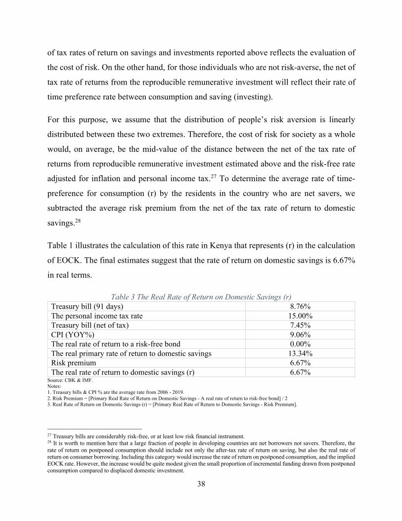
Table 1 illustrates the calculation of this rate in Kenya that represents (r) in the calculation
of EOCK. The final estimates suggest that the rate of return on domestic savings is 6.67%
in real terms.
Table 3 The Real Rate of Return on Domestic Savings (r) Treasury bill (91 days) 8.76% The personal income tax rate 15.00% Treasury bill (net of tax) 7.45% CPI (YOY%) 9.06% The real rate of return to a risk-free bond 0.00% The real primary rate of return to domestic savings 13.34% Risk premium 6.67% The real rate of return to domestic savings (r) 6.67%
Source: CBK & IMF. Notes: 1. Treasury bills & CPI % are the average rate from 2006 - 2019. 2. Risk Premium = [Primary Real Rate of Return on Domestic Savings - A real rate of return to risk-free bond] / 2 3. Real Rate of Return on Domestic Savings (r) = [Primary Real Rate of Return to Domestic Savings - Risk Premium].
27 Treasury bills are considerably risk-free, or at least low risk financial instrument. 28 It is worth to mention here that a large fraction of people in developing countries are net borrowers not savers. Therefore, the rate of return on postponed consumption should include not only the after-tax rate of return on saving, but also the real rate of return on consumer borrowing. Including this category would increase the rate of return on postponed consumption, and the implied EOCK rate. However, the increase would be quite modest given the small proportion of incremental funding drawn from postponed consumption compared to displaced domestic investment.

39
2.3.1.3 The Marginal Economic Cost of Foreign Financing (567) in Kenya
The marginal cost of foreign borrowing is the third element we need for the estimation of
the EOCK. In an open economy, when the government accesses the world capital market,
raising funds stimulates the savings of foreigners to inflow into the economy. In particular,
the higher demand for foreign funds will increase the interest rate faced by the country in
the international capital markets, which implies that the higher rate will be paid not only
on the extra borrowing demanded by the project but also on all the debt contracted by the
country at variable interest rates.
Therefore, for the economy as a whole, the economic cost of foreign borrowing is not given
by the interest rate faced by the incremental project, which represents the average cost of
borrowing, but by the cost of funds faced by the project plus the extra cost generated on
the existing debt, which represents the marginal cost of borrowing.
With the existence of a country risk premium, Edwards (1986) discusses that the country
faces an upward sloping supply curve of foreign borrowing, and public projects impact the
relevant marginal cost of foreign indebtedness. Therefore, the marginal economic cost of
foreign funds is increasing above the average cost of foreign funds.
The marginal cost of foreign borrowing created by the projects can be calculated as follows:
89# =-.#∗(('!%)'*2#3
(+*2#∗ ;1 + # ∗ <
(4&#=> (7)
Equation (7) indicates that the 56! is determined by is the average nominal interest rate
charged on external loans, ?#, tw is withholding tax rate on interest income, @A# is the foreign
inflation rate, # the proportion of foreign debt contracted in a floating interest rate, B&# is
the elasticity of the supply of foreign funds with respect to the interest rate.
According to the World Bank, International Debt Statistics, the outstanding amount of
long-term external debts of Kenya was at 34,217.10 million US dollars in 2019, in which

40
30,069.10 million US dollars is held by public and publicly guaranteed institutions. The
currency composition of PPG debt shows that the US dollar-denominated long-term PPG
debt accounts for 72% on average of the total for the last five years.29 Accordingly, we
consider that @A# in equation (7) is the GDP deflator of the United States. Taking the
average U.S. annual inflation rates throughout the study period, the @A" equals 1.80%.
Regarding the proportion of foreign financing that is responsive to interest rate changes,
World Bank, International Debt Statistics provide the percentage of long-term external debt
with interest rates that float with movements in a key market rate. Over the last five years,
the variable interest rate accounts for around 31.36% of the external debt stocks in Kenya.
For this analysis, we assume that this ratio represents the share of foreign borrowing
responsive to interest rate changes (K).
With the purpose of finding the cost of foreign lending to domestic borrowers (?C), we
estimate that the interest rate charged on foreign financing would be at least the U.S.
treasury long-term rate plus an additional charge for country risk. The U.S. treasury's long-
term average nominal interest rate is about 2.33%.30 Using Damodaran's (2020) estimation
of country risk premium, we obtained the estimated cost of foreign borrowing for Kenya
net of withholding tax at 7.66%.31
The last component required for equation (7) is the elasticity of the supply of foreign funds
with respect to the interest rate. This variable is set at 2; however, a sensitivity test has been
29 According to the World Bank, International Debt Statistics, around 75.5% of the long-term external debt in 2019 is denominated in US dollar, 11% in other currencies, 7.3% in Euro, and 4.6% in Japanese Yen. 30 Source of U.S. Treasury Long-Term Average Rate data is U.S. Department of the Treasury. Long term treasury represents a treasury with 25 years or more remaining to maturity. We consider the annual average rate of U.S. treasury long-term in the last five year (2016-2020) as we are concerned with the apprising of public project in the future. 31 It is worth to mention here that Gueye & Sy (2015) estimated the interest rate cost of external borrowing from international capital market for Kenya at 7.65%. Another indicator that may reflect the cost of government borrowing from abroad is sovereign bonds issued in US dollars in international market. Information about Eurodollar bonds are collected from DataStream and it shows that Kenya raised $2 billion of 5 years and 10-year Eurobond in 2014 with coupon rates 5.875% and 6.875%. Moreover, in 2018 Kenya issued another $2 billion Eurobond of 10 years and 30 years with coupon rates 7.250% and 8.250%.

41
undertaken to define the effect of changes in this parameter on the estimation of the
economic opportunity of capital.32
Substitution the parameters and assumptions describe in equation (7), the estimate of the
real marginal economic cost of foreign financing (89") for Kenya is at 6.65%.
2.3.2 Shares of the Three Diverted Funds in Financing the Projects
After we estimated the cost for each of the three components of EOCK, the next step is to
assess the weights of each of the three sources of funds. According to Jenkins et al. (2019),
the weights of each source of funding related to “the average contributions made from each
source and their price responsiveness to the change in market interest rate as a result of
raising funds for a new investment project in the capital market.” For empirical estimation,
the relevant formulas of Jenkins & Kuo (1998) can be followed:
(8)
(9)
(10)
Where, = the elasticity of the supply of foreign funds; h = elasticity of demand for
private investment = supply elasticity of household savings; in response to the interest
32 It is worth noting that the elasticity of the supply of foreign funds has two compensating effects: to the extent that it increases the share of foreign funding, yet the marginal cost of these funds decreases.
)()()(
)(1
t
t
t
fsf
t
dsh
t
t
SI
SS
SS
SI
fhee
h
-+
-=
)()()(
)(2
t
t
t
fsf
t
dsh
t
dsh
SI
SS
SS
SS
fhee
e
-+=
)()()(
)(3
t
t
t
fsf
t
dsh
t
fsf
SI
SS
SS
SS
fhee
e
-+=
sfe
she

42
rate changes. St = total private-sector savings available in the economy; Sd = total domestic
savings; and Sf = total net foreign capital inflows; It = private sector investment.
As noted in the preceding part, the supply elasticity of foreign funds has been set at 2 in
Kenya. Based on Ogaki et al.'s (1996) estimations, the average interest sensitivity of
savings at an initial real interest rate of 3% was about 0.312 in low-income countries, while
it was about 0.532 for the lower-middle-income countries. For this study, we use 0.4 as the
supply elasticity of private savings in our calculations. The interest elasticity of demand
for domestic investment is set at -1.0.
The International Monetary Fund (IMF) Government Finance Dataset shows that the
general government net lending/borrowing account is negative throughout the study period
in Kenya. Hence, one can say that a major part of domestic savings is private-sector
savings, and the private-sector investment in Kenya have been financed by private sector
savings. In this regard, we consider (It/St) is the average ratio of private sector investments
to private sector savings. According to recently available data, the ratio of total private-
sector investment to total savings would be approximately 77.37% which is used for (It/St)
in this analysis.33
The amount of foreign investment includes the stock of foreign direct investment (FDI)
and the stock of long-term external debt. Using the 2019 figures, the total amount of foreign
investment at 2009 constant prices was KES 2,465,672 million (USD 24,171.74 million).
This amount was financed through foreign savings. The ratio of this foreign financing to
total reproducible capital is about 20.80%. Over the period of this study, the average share
of foreign financing to the total reproducible capital (Sf/St) is estimated at 14.31%; thus
the 85.69 would be financed by domestic savings. (see Appendix D).
33 This ratio represents the period from 2015 to 2020. Data are obtained from IMF Country Report No. 21/72. Requests for An Extended Arrangement Under the Extended Fund Facility and An Arrangement Under the Extended Credit Facility—Press Release; Staff Report; And Statement By The Executive Director For Kenya.
43
With these rations and assumptions, the shares of funds diverted from the three sources
described above can be derived. They are 55.16% from displaced or postponed domestic
investment, 24.44% from domestic savings, and 20.41% from additional foreign capital
Inflows.
2.3.3 Estimates for the EOCK
The estimation of EOCK now is carried out as a weighted average rate of return to
displaced reproducible remunerative capital investment and the rate of return on domestic
and foreign savings. These rates and the corresponding weight for each one are obtained in
the previous sections. By applying equation (1), the economic discount rate of Kenya is
estimated at 11.36%.
2.3.4 Sensitivity Analysis
One of the challenges for measuring the EOCK for Kenya relates to the availability of data
required for estimation. When the data are not available, they are based on our observation
of the economic indicators elsewhere. The empirical results in the base case depend on the
values of several key parameters, including the share of labor income in GDP, the
depreciation rates used for estimating the total capital stock, the percentage share of the
remunerative portion of investment in total capital stock, the elasticity of demand for
domestic investment, and the supply elasticity of household savings. We conduct a
sensitivity analysis regarding the impact of these key parameters on the estimate of the
economic opportunity cost of capital.
i. The Share of Labor Income in GDP
If the proportion of labor income in GDP is 3 percent less than the base case illustrated in
appendix A (Column 3), the real rate of return to domestic investment would be raised on
average to 17.4% over the past fourteen years, and the time preference of consumption to
8.90%. Using 16.9% for ρ, 8.4% for r, and 6.65% for MCf, the EOCK becomes about 12.7
percent, 1.34 percentage points higher than that for the base case.
44
On the other hand, if the portion of labor income in GDP is 3 percentage higher than the
base case, the average rate of return to domestic investment and the time preference of
consumption would be reduced to 13.5% and 5%, respectively. As a consequence, the
EOCK decreases to 10.02 percent, which is 1.34 percentage points lower than that for the
base case.
ii. Depreciation Rates
a. Annual Depreciation Rate for Residential and Non-Residential Structures
If the depreciation rate used for the capital stock of residential and non-residential
structures is 2.0% instead of 2.5%, the parameters ρ and r are calculated to be 14.4% and
6 %, respectively. Substituting these opportunity costs of funds along with 6.65% for MCf
in equation (1) yields the EOCK at 10.76%.
On the other hand, if the depreciation rate is assumed higher at 3.0%, the values of ρ and r
are estimated higher at 15.9% and 7.3%, respectively, compared to the previous cases.
Accordingly, the EOCK would be slightly increased to 11.92 percent, 0.56 of one
percentage point higher than that for the base case.
b. Annual Depreciation Rate for Machinery, Transport Equipment, and Other Assets
If the depreciation rate used for the capital stock of machinery, transport equipment, and
other assets is 4.0% instead of 6%, the parameters ρ and r are calculated to be 13.66% and
5.33%, respectively. Substituting these opportunity costs of funds along with 6.65% for
MCf in equation (1) yields the EOCK at 10.19%.
On the other hand, if the depreciation rate is assumed higher at 8.0%, the values of ρ and r
are estimated higher at 16.35% and 7.7%, respectively, compared to the previous cases.
Accordingly, the EOCK would be increased to 12.26 percent, 0.90 of one percentage point
higher than that for the base case.
45
iii. The portion of Capital Stock Attributable to the Remunerative Capital
If the share of the remunerative portion of capital stock is adjusted upward to 76% of total
capital stock from the base case at 73%, the average rate of return to domestic investment
falls to 14.6%, so does the time preference of consumption to 6.1%. Using 14.6% for ρ,
6.1% for r, and 6.65% for MCf, the EOCK is estimated at about 10.90 percent, 0.46
percentage points lower than that for the base case.
Suppose the portion of capital stock attributable to the remunerative is adjusted downward
to 70%. The EOCK would be 11.86 percent.
iv. Elasticity of Demand for Domestic Investment
If the price elasticity of demand for domestic investment is -0.5 instead of the base case
value of -1, the share of funds sourced from displaced private investment becomes smaller,
and the EOCK would be reduced to 9.91 percent. On the other hand, if the price elasticity
of demand for domestic investment is -1.5, the EOCK will increase to 12.19 percent, owing
to the larger share of funds diverted from domestic remunerative investment sources.
v. Supply elasticity of household savings
If the supply elasticity of savings by households is assumed at 0.2 rather than 0.4 assumed
for the base case, the EOCK in Kenya will increase by 0.65 of one percentage point.
However, if this variable is set at 0.6 instead of 0.4, the EOCK will decrease by
approximately 0.51 of one percentage point.
From the above sensitivity analyses, we find the estimates of the ECOK range from 9.91
percent to 12.7 percent, as shown in Table 2. Taking into consideration the results of all
extreme cases, the average would be 11.3%. Given the data obtained and used for the
analysis, these results suggest that an 11.5 percent real rate is an appropriate and
conservative discount rate to be used to discount annual real resource costs and economic
benefit over the life of an investment project.
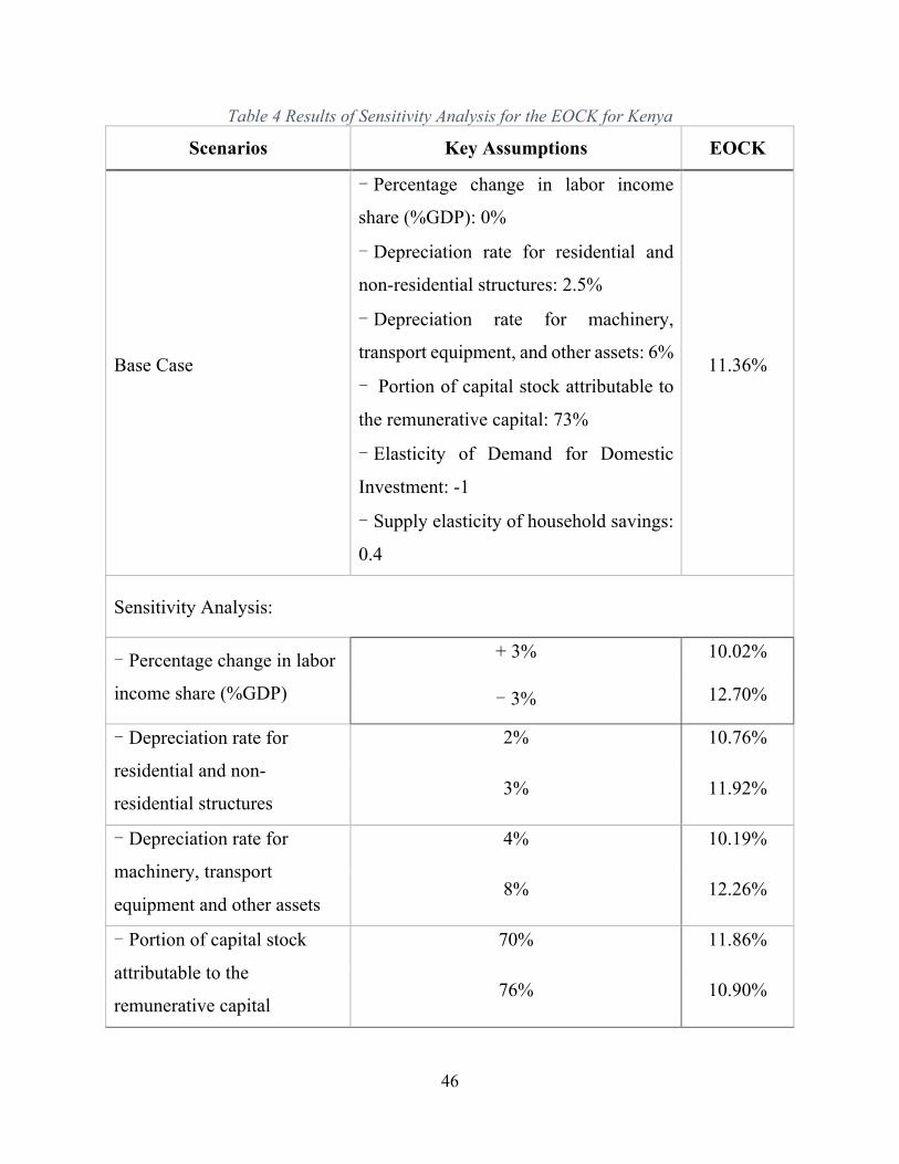
46
Table 4 Results of Sensitivity Analysis for the EOCK for Kenya
Scenarios Key Assumptions EOCK
Base Case
- Percentage change in labor income
share (%GDP): 0%
- Depreciation rate for residential and
non-residential structures: 2.5%
- Depreciation rate for machinery,
transport equipment, and other assets: 6%
- Portion of capital stock attributable to
the remunerative capital: 73%
- Elasticity of Demand for Domestic
Investment: -1
- Supply elasticity of household savings:
0.4
11.36%
Sensitivity Analysis:
- Percentage change in labor
income share (%GDP)
+ 3% 10.02%
- 3% 12.70%
- Depreciation rate for
residential and non-
residential structures
2% 10.76%
3% 11.92%
- Depreciation rate for
machinery, transport
equipment and other assets
4% 10.19%
8% 12.26%
- Portion of capital stock
attributable to the
remunerative capital
70% 11.86%
76% 10.90%
47
- Elasticity of Demand for
Domestic Investment
-0.50 9.91%
-1.50 12.19%
- Supply elasticity of household savings
0.20 12.01%
0.60 10.85%
3 Measurement of the FEP and NTP
3.1 Introduction
An issue that must be decided before doing any project appraisal has to do with the unit of
measurement or numeraire. In principle, economic project analysis can be conducted in
domestic or foreign currency and at domestic or border (world) price levels. However, the
most common path is to use domestic currency and domestic price levels as the numeraire.
This implies that tradable goods and services prices are taken at the world price and
converted into domestic currency at an economic price of foreign exchange.
In general, economic prices differ from market prices as a consequence of the pervasive
existence of trade and other indirect tax and subsidy distortions. In other words, there are
important fiscal impacts that are not captured by a project when funds are taken out from
the rest of the economy for the purchase of inputs. The opposite phenomena take place
with the production of the outputs of any project.
The standard treatment of the economic price of foreign exchange is based on the thought
that when the goods purchased as inputs are tradable goods, it will increase the demand for
foreign exchange in the foreign exchange market. The premium on the foreign exchange
rate (FEP) needs to be quantified and included in the analysis. However, when resources
are used to buy non-tradable (domestic) goods, there is a fiscal impact associated with the
non-tradable outlays because of the set of taxes and subsidies that cause the shadow price
of non-tradable goods to be greater or less than their financial values.

48
These actions are repeated many times for each project and are identical for such actions
across projects. Therefore, it is more efficient to estimate these variables once for a country
and use the same values repeatedly as needed in the appraisal of all projects in Kenya.34
These premiums are best expressed as a percentage of the market foreign exchange rate
and the financial value of non-tradable goods, respectively. They can be easily incorporated
in the economic evaluation of project projects from the analysis of the financial
evaluation.35
3.2 Analytical Framework
The conceptual framework employed to measure these premiums is based on a three-sector
general equilibrium model in an economy developed by Harberger and Jenkins.36 The three
sectors of this model consist of importable, exportable, and non-tradable goods. Both
importable and exportable goods are part of tradable goods. 37
One advantage of the new approach elaborated by Harberger and Jenkins is that it does
consider not only internal distortions but also the intratemporal repercussions of the way
in which funds of the project (used to buy foreign exchange) are raised so that the
incremental demand of foreign exchange will be accommodated not only by movements
along the demand and supply of foreign exchange but also by shifts in both curves.
This framework was further developed by Kuo, Salci, and Jenkins into an operational guide
and empirically applied to several countries in Africa.38 This model is employed here to
measure the FEP and the NTP for Kenya.
34 The variables are not estimated in a way to be specific to a particular commodity or project. 35 See, e.g., Jenkins, G., Kuo, C., & Harberger, (2019) 36 Harberger, A. C., & Jenkins, (2002) 37 Importable goods include the goods and services that are actually imported plus the domestically produced goods that are substitutes for these imports. Exportable goods include the goods and services that are produced and could also be consumed domestically. Non-Tradable goods are the goods that are only produced and consumed domestically. 38 Kuo, Salci, and Jenkins, (2015).

49
Kenya is open and integrated into the global market economy. When project funds are
sourced in the capital market, they are sourced domestically as well as abroad, as described
in Section II. If funds are sourced domestically and used to purchase a project’s tradable
goods, there will be a displacement or postpone of domestic investment and consumption
expenditures, which reflect a reduction of demand for domestic tradables and non-
tradables. The net result is an excess demand for tradables and excess supply of non-
tradables in the economy. The consequence is forgone indirect taxes and subsidies
associated with changes in the above expenditures, which reflects an increase in the welfare
cost of using the foreign exchange to purchase tradable inputs (i.e., ∆EFt,d).39
This will not be the case, however, when funds are sourced abroad and spent on tradable
goods as the financing is obtained entirely in foreign currency and since the prices of all
tradables are measured in foreign currency, there is no market adjustment when funds are
obtained abroad and spent entirely on tradables because there is no excess domestic
demand for foreign exchange nor is an excess demand for domestic currency and
expenditures (tradable and non-tradable) in the economy. Thus, no additional welfare cost
will occur. That is, ∆EFt,f = 0.
Although project funds are initially raised in the domestic market, they will ultimately end
with funds sourced domestically and abroad when equilibrium is re-established.
Hence, the impacts of the two market operations create a net welfare cost, which is termed
the FEP and can be calculated in a weighted average as follows:
FEP = Gd ∙ ∆EFt,d + Gf ∙ ∆EFt,f
=Gd ∙ ∆EFt,d (11)
39 Detailed explanation can be found in Kuo, Salci, and Jenkins (2015).

50
where Gd and Gf stands for the proportions of funds sourced domestically and abroad,
respectively.
When project funds are raised in the domestic market but spent on non-tradable goods, the
excess demand for non-tradables and excess supply of tradables would occur and generate
a net welfare cost. However, if foreign funds are used to spend on non-tradable goods, there
is no initial displacement of investment and consumption of tradables and non-tradables
owing to the capital extraction. Thus, the excess demand for non-tradables and excess
supply of tradables will be greater than the previous case because of a larger impact on the
real exchange rate when a new equilibrium is established.40 The net welfare cost (or NTP)
in the economy can be measured by the weighted average of the changes in economic
welfare as a result of funds either sourced in the domestic market (∆EFnt,d) and the
foreign market (∆EFnt,f):
NTP = Gd ∙ ∆EFnt,d + Gf ∙ ∆EFnt,f (12)
3.2.1 Measuring the Foreign Exchange Premium
To measure the FEP and the NTP, the first is to find out the proportions of project funds
sourced domestically and abroad (i.e.,Gd andGf) and to estimate various welfare costs
associated with each sourced fund. The proportions of project funds have been dealt with
in Section II.41 This section focuses on how each of the welfare costs can be estimated.42
Funds Sourced Domestically are Spent on Tradable Goods
We begin with the net welfare cost when funds are extracted from the domestic capital
market to finance the purchase of tradable goods, and then the consequential effect (i.e.,
substitute effects) will take place due to the impact of changes in the relative price of
40 When the funds are used entirely to purchase non-tradable goods, these foreign exchanges must be first converted into a domestic currency as the prices of non-tradables are given in domestic currency. Therefore, the demand for tradables will increase and the supply of tradables will decrease as the relative price of non-tradable versus tradable increases. 41 The sourcing of funds here is consistent with the ones estimated in the EOCK 42 Most of this section and Sections 3.2.2 are taken from Kuo, Salci and Jenkins (2015). It is presented here for the benefit of readers.

51
tradable to non-tradable goods. First, when project funds are extracted from the capital
markets, this act will reduce the expenditures made by other businesses and consumers on
tradables and non-tradables. The decrease in the demand for tradables and non-tradables
will reduce the amount of value-added tax (VAT) as well as excise taxes on specific goods
and services. In the case of VAT, businesses will be credited for the tax paid on the
purchases of business inputs to offset the VAT liabilities from their sales. As a result, only
(1-!i) of the displaced expenditures will affect VAT payments, where !i refers to the
proportion of expenditures during the capital market extraction that is excluded from VAT
because of the input tax credit.
The effective VAT rates are different between tradable and non-tradable goods because the
portions of their respective goods excluded from VAT differ considerably. If vt and vnt
stand for the effective VAT rates on demand for tradables and non-tradables, respectively,
only vt (1-!i) and vnt (1-!i) of the displaced expenditures from the capital market operation
will affect the tax payments. This is shown in the first two terms of equation (13), where
and are the reductions in the demand for tradables and non-tradables
as a result of funds sourced through the domestic capital market extraction,∆ . Using the
domestic currency as a numeraire, the real exchange rate, E, reflects the relative price of
tradable to non-tradable goods.
(13)
In the case of excise duty imposed on selected goods, they are not creditable even if
purchased for businesses. This effect is captured in the third term of equation (13). Thus,
captures the total impact on the welfare cost that is due to changes in VAT and
excise duties collected over the process of the extraction of funds from the domestic capital
market.43
43 The impact of excise taxes on tradables is captured in equation (15), below.
∂Qd,t ∂FD ∂Qd,nt ∂F
D
DF
ΔEW1 = vt 1− ρi( )∂Qd,t
∂FD
$
%&
'
()E + vnt 1− ρi( )
∂Qd,nt
∂FD
$
%&
'
()+ te,nt
∂Qd,nt
∂FD
$
%&
'
()
*
+,
-
./dFD
1EWD

52
If the sourced funds are totally spent on tradables, this will initially create a net excess
demand for tradables and a net excess supply of non-tradable goods in the economy. This
disequilibrium situation will cause a rise in the relative price of tradables to non-tradables;
the process will continue until a new equilibrium is reached in which no excess supply
exists in the tradables sector owing to adjustments of the real exchange rate. The resources
required to produce the additional tradables will come from the reduction in the production
of non-tradables. Equilibrium is again established when the sum of the total demand for
tradabes (Qd,t) and non-tradables (Qd,nt) equals the total supply of tradables (Qs,t) and
non-tradables (Qs,nt) plus any of the trade deficit that is financed in the form of
remittances, foreign aids and foreign investment.
Given the resource constraint, the above mechanism operates through the adjustment in the
real exchange rate.44 As a consequence of the adding-up properties of demand in a two-
good economy, the compensated own-price elasticity of demand for tradables must
be equal to the compensated cross-price elasticity of demand for non- tradables times
the ratio of the demand for non-tradables to tradables (Qd,nt /Qd,t). Similarly, for the
supply side, the own-supply elasticity ( ) should be equal to the cross-supply elasticity of
non-tradables ( ) multiplied by the ratio of the supply of non-tradables to tradables (Qs,nt
/Qs,t).
Since the change in the real exchange rate is required to restore equilibrium in the markets,
a change in welfare cost will come about by the interaction of tax and subsidy distortions
with the changes in the quantities demanded and supplied. These substitution effects on the
welfare cost can be measured by equation (14). The first term refers to the change in VAT
collected and subsidy on production in the tradable goods, while the second term is the
change in VAT and excise taxes collected and subsidy on production in the non-tradable
goods sector.
44 Alternatively, there will be an excess supply of tradable goods if the funds are all spent on non-tradable goods. The case will be presented in the next section.
( )dth( )dnth
ste
snte
53
(14)
where and are the production subsidies on tradables and non-tradables,
respectively; and is the proportion of the changes in demand resulting from the exchange
rate adjustment that is excluded from VAT.
In addition to the domestic VAT and excise taxes, there are other external trade distortions,
such as import duties, excise duties, and export taxes associated with changes in imports
and exports. The effects of these changes on welfare cost over the capital extraction are
measured by the third component ( ):
(15)
where tm is the effective import duty rate, tx is the effective export tax rate, te is the effective
excise tax rate on tradable goods. Qd,i is the demand quantity of importable goods, and
Qd,e is the quantity of exportable goods demanded domestically.
The fourth component ( ) accounts for welfare cost caused by trade distortions due
to the substitution effects. This can be measured in equation (16):
(16)
where is the own-price supply elasticity of exports, is the own-price demand
elasticity of imports, is the amount of exports, and is the amount of imports.
Suppose the amount of funds raised in the economy is one unit of a foreign country, the
FEP can be measured by substituting the welfare costs calculated from equations (13), (14),
(15), and (16) into equation (11) as follows:
ΔEW2 =vt 1− ρs( )ηt
d
εts −ηt
d −ktεt
s
εts −ηt
d
#
$%%
&
'((E +
vnt 1− ρs( )ηntd
εts −ηt
d +te,ntηnt
d
εts −ηt
d −kntεnt
s
εts −ηt
d
#
$%%
&
'((Qd,nt
Qd,t
#
$%%
&
'((
)
*++
,
-..1+ ∂Qt
∂FD
#
$%
&
'(dFD
tK ntK
sr
3EWD
ΔEW3 = tm∂Qd,i
∂FD
#
$%
&
'(+ te 1+ tm( )
∂Qd,i
∂FD
#
$%
&
'(+ tx
∂Qd,e
∂FD
#
$%
&
'(
)
*+
,
-.(E)dFD
4EWD
ΔEW4 =tmηM
d QMd /Qd,t( )
εts −ηt
d
⎛
⎝⎜⎜
⎞
⎠⎟⎟+
te 1+ tm( )ηMd QM
d /Qd,t( )εts −ηt
d
⎛
⎝⎜⎜
⎞
⎠⎟⎟−
txεXs QX
s /Qs,t( )εts −ηt
d
⎛
⎝⎜⎜
⎞
⎠⎟⎟
⎡
⎣
⎢⎢
⎤
⎦
⎥⎥E( ) 1+
∂Qd,t
∂FD
⎛
⎝⎜
⎞
⎠⎟dFD
sXe
dMh
QXs QM
d
54
FEP = Gd ∙ [ + + + ] (17)
3.2.2 Measuring the Premium for Non-tradable Outlays
The NTP is a premium equivalent to the FEP that is associated with non-tradable outlays.
It is the amount in which the economic cost of non-tradable outlays exceeds the financial
outlays. What follows is to estimate the forgone taxes or welfare cost as a result of raising
each of the funds sourced either domestically or abroad.
Domestic Funds are Spent on Non-tradable Goods
In this case, the initial impacts of the capital extraction will have the same effects as
expressed in equations (13) and (15) for the estimation of the FEP.
When funds are spent on non-tradables, there will be an excess demand for non-tradables
and an excess supply of tradables. This will cause the relative price of non-tradables to
tradables to increase. The adjustment process will continue until the excess demand for
non-tradables is eliminated.
The impacts on economic welfare due to the substitution effects are two-fold. The first is
the change in welfare cost ( ) associated with changes in the demand and supply of
tradable goods whose markets contain domestic indirect taxes and production subsidies
and the second effect ( ) is associated with changes in imports and exports that are
subject to external trade taxes. They can be measured as follows:
(18)
(19)
1EWD 2EWD 3EWD 4EWD
ΔEW5
6EWD
ΔEW5 =vt 1− ρs( )ηt
d
εts −ηt
d −ktεt
s
εts −ηt
d
#
$%%
&
'((E +
vnt 1− ρs( )ηntd
εts −ηt
d +te,ntηnt
d
εts −ηt
d −kntεnt
s
εts −ηt
d
#
$%%
&
'((Qd,nt
Qd,t
#
$%%
&
'((
)
*++
,
-..
∂Qt
∂FD
#
$%
&
'(dFD
ΔEW6 =tmηM
d QMd /Qd,t( )
εts −ηt
d
⎛
⎝⎜⎜
⎞
⎠⎟⎟+
te 1+ tm( )ηMd QM
d /Qd,t( )εts −ηt
d
⎛
⎝⎜⎜
⎞
⎠⎟⎟−
txεXs QX
s /Qs,t( )εts −ηt
d
⎛
⎝⎜⎜
⎞
⎠⎟⎟
⎡
⎣
⎢⎢
⎤
⎦
⎥⎥E( )
∂Qd,t
∂FD
⎛
⎝⎜
⎞
⎠⎟dFD

55
The total welfare cost, in this case, can be measured by the sum of , , ,
and .
Foreign Funds are Spent on Non-tradable Goods
When foreign funds are sourced, there is no impact on the domestic economy. Until the
funds are spent on non-tradables, an additional demand for non-tradables will cause an
increase in the relative price of non-tradables to tradables. The impact in this case is greater
than when funds are sourced domestically and spent on non-tradables, since there is no
initial displacement of domestic investment and consumption in non-tradable goods to be
offset. Consequently, the supply of non-tradables will expand much more, demanding
greater resources to come to the sector from the tradable good sector.
There is only a substitution effect in this case. These effects can be separated into two parts.
The first is the change in welfare cost ( ) associated with changes in quantities of
items that have domestic taxes and production subsidies levied on them, while the second
part ( ) is the change in trade taxes associated with the changes in demand and supply
of tradable goods when these goods cross borders. These effects can be calculated as
equations (20) and (21), respectively:
(20)
(21)
The total welfare cost, in this case, is simply the sum of and .
Since the funds used for the projects are sourced domestically as well as abroad, the NTP
should be estimated as a weighted average of the welfare costs associated with each source
1EWD ΔEW3 ΔEW5
ΔEW6
ΔEW7
ΔEW8
ΔEW7 =vt 1− ρs( )ηt
d
εts −ηt
d −ktεt
s
εts −ηt
d
#
$%%
&
'((E +
vnt 1− ρs( )ηntd
εtd −ηt
d +te,ntηnt
d
εts −ηt
d −kntεnt
s
εts −ηt
d
#
$%%
&
'((Qd,nt
Qd,t
#
$%%
&
'((
)
*++
,
-..
∂Qt
∂FF
#
$%
&
'(dFF
ΔEW8 =tmηM
d QMd /Qd ,t( )
ε ts −ηt
d
⎛
⎝⎜
⎞
⎠⎟ +
te 1+ tm( )ηMd QM
d /Qd ,t( )ε ts −ηt
d
⎛
⎝⎜
⎞
⎠⎟ −
txε Xs QX
s /Qs,t( )ε ts −ηt
d
⎛
⎝⎜
⎞
⎠⎟
⎡
⎣⎢⎢
⎤
⎦⎥⎥E( ) ∂Qs,t
∂FF⎛⎝⎜
⎞⎠⎟dFF
ΔEW7 ΔEW8

56
of funds. This can be done by substituting the welfare costs calculated from equations (13),
(15), (18), (19), (20), and (21) into equation (12). That is:
NTP = Gd ∙ ∆EFnt,d + Gf ∙ ∆EFnt,f
= Gd ∙ [ + + + + ] + Gf ∙ [ + ] (22)
3.3 Empirical Estimation
The analytical framework and equations for measuring the FEP and NTP were presented
in the previous section. We need to estimate all variables for Kenya. They can be grouped
into four categories. The first is the proportion of funds sourced domestically and abroad
in order to finance the purchase of tradable and non-tradable goods. The second is the
relative sizes of tradable and non-tradable goods in order to measure the interrelated
impacts between tradable and non-tradable sectors. The third is the demand and supply
elasticities of imports, exports, and non-tradable goods with respect to the real exchange
rate. The last is the effective tax rate for each of the major indirect taxes and the effective
rates of production subsidies.
3.3.1 Alternative Sources of Funds
The source of funds used to finance projects has a significant impact on the estimated
values of the FEP and the NTP. This is due to the fact that if sourced in the domestic capital
market, the funds will displace expenditures on investment and final consumption, whereas
no such displacement of expenditure occurs if the funds are sourced abroad.
As shown in Section II, when funds are raised in the capital market in Kenya, the
proportions of funds diverted to finance investment projects in the base case are 24.44%
from domestic savings, 55.16% from displaced domestic investment and 20.41% from
foreign savings. The first two components constitute domestic sources of funds, while the
third component represents the foreign source of funds. In other words, Gd and Gf are
79.59% and 20.41%, respectively, for equations (11) and (12).
1EWD 3EWD ΔEW5 ΔEW6 7EWD 8EWD
57
3.3.2 Tradables vs Non-tradables
The relative size of tradable and non-tradable goods in the economy has important
implications for the FEP and the NTP because of the different scope of VAT and other
product taxes imposed on these goods and services. At present, the agriculture and industry
sectors account for 35.15% and 16.17% of GDP, respectively, in Kenya.45 Virtually all of
these products are moveable and tradable. The service sector is the biggest sector in which
trade, restaurants, hotels, information and communication, professional services, and
associated transportation and food service activities account for approximately 19.7% of
GDP, and many of these services are closely related to tradable goods.
For the country as a whole, we have estimated that the tradable and non-tradable goods in
Kenya are approximately two-thirds and one-third, respectively. This is in line with an
estimate based on the economy for South Africa using data with a detailed commodity
breakdown.46
Like most African countries, Kenya has been in a trade deficit position for years. According
to World Bank national accounts data, the trade balance in Kenya is on average (-11.71%)
of GDP over the period of this study.47 This suggests that the share of the demand for
importables is much greater than that of exportables, and thus, the importable demand is
assumed to represent a much greater share of total tradables than exportable demand. For
the purpose of this study, the demand for importables as a share of total demand for
tradables in an economy is assumed to be 80%, while the domestic supply of importables
as a share of a total supply of tradables is 35%. This implies that the proportion of the
domestic demand and the supply of exportables in the total demand and supply of tradables
would be 20% and 65%, respectively.48
45 World Bank, World Development Indicators (2020). 46 See, e.g., Harberger, Jenkins, Kuo and Mphahlele (2003). 47 See, https://data.worldbank.org/indicator/NE.RSB.GNFS.ZS?locations=KE 48 The latest available Supply and Use Tables, 2017 for South Africa, shows that the domestic supply of importables as a share of a total supply of tradables is 49%. We would expect that this share to be smaller in Kenya because of a lesser open and economic development.
58
With regard to assessing the impact on the economy of the capital extraction alone, the
proportion of importables can be more than the 80% that is assumed for the economy as a
whole because tradable goods make up a larger share of total investment. In Kenya, of the
displaced investment business, inputs such as motor vehicles, machinery, telecom
equipment, and others are all imported. Accordingly, the demand for importables as a
proportion of the total demand for tradable capital formation could be as high as 95%, or
85%, at a conservative estimate. Thus 90% of displaced investment is assumed to be
importable. As regards tradable consumption, 80% is assumed to be importables, the same
proportion as for the economy as a whole. According to Section II, about 55.16% of funds
are sourced from the displacement of investment and 24.44% from consumption forgone
in response to stimulated household savings over the capital extraction. Hence, about
86.93% of the total change in the demand for tradables caused by the capital market
extraction would be importable.49
3.3.3 Demand and Supply Elasticities
The demand and supply elasticities of tradable or non-tradable goods are important for
quantifying the response of their demand and supply to the relative price of tradable to non-
tradable goods (or the change in the real exchange rate). Given the resources available in
the economy, in order to ensure the market equilibrium, the derived compensated own-
price elasticity of demand for tradables must be equal to the compensated cross-price
elasticity of demand for non-tradable multiplied by the ratio of the demand for non-
tradables to the demand for tradables. The cross-price elasticity of the supply of non-
tradables multiplied by the ratio of the supply of non-tradables over the supply tradables is
equal to the negative of the own-price supply elasticity of tradables.
Precise estimates of demand (or supply) elasticities of tradables and non-tradables are not
readily available in the literature. But the sum of the own-price elasticities of demand for
49 This is estimated as a weighted average of importables as a share of total demand for tradables of both household consumption expenditures and business investment. That is, 86.93% = (0.2444* 80% + 0.5516*90%)/ (0.2444 + 0.5516) = 0.3070*80% + 0.6931*90%.
59
tradables and non-tradables must be equal to the elasticity of substitution (defined
negatively) between tradables and non-tradables.
For the purpose of this study, we consider it reasonable to assume an elasticity of
substitution of -1.0 between the use of tradables and non-tradables in the economy. In this
world of two composite goods, the own-price elasticities of demand will be inversely
proportional to their shares in total demand. Hence, if the share of tradables is 2/3 and the
share of non-tradables is 1/3 of the total demand and the elasticity of substitution is equal
to -1.0, then when trade is balanced, the own-price elasticities of demand for tradables and
non-tradables must equal -0.33 and -0.67, respectively.
However, the size of the trade deficit in a country will expand the country’s expenditures
on tradable goods and hence requires an adjustment to the relative size of the two own-
price elasticities of demand. The reverse is true for a trade surplus. According to the current
account of the balance of payments information, Kenya had a trade deficit over the period
from 2006 to 2019 ranging from 8.9% to 17.2% of gross domestic product. The own-price
demand elasticity of tradables is adjusted slightly from –0.33 to –0.295, and the own-price
elasticity of demand for non-tradables will become –0.705. On the supply side, the price
elasticities of supply of exportables and importables are assumed to be +1.0, while the own-
price supply elasticity of tradables will also be +1.0.
In order to quantify the effects on the amount of import duties and export taxes, we need
to determine the compensated own-price elasticity of demand for imports and the
supply elasticity of exports .
The simple and weighted averages of import demand elasticity were estimated for Kenya
at -1.89 and -1.14 by Kee, H. L et al. (2008). For the purpose of this study, we assume that
the import demand elasticity for Kenya is a midpoint between those two averages at -1.52.
The export elasticity of supply as estimated by Tokarick (2014) represents the average
long-run export supply elasticity adjusted to include the general equilibrium effects of price
( )ste
( )dMh( )sXe

60
changes. For Kenya, the supply elasticity of exports is calculated at 0.57. A sensitivity
analysis will be undertaken for these key variables later.
3.3.4 The Effective Tax and Subsidy Rates
The major distortions involved in the estimation of the FEP and the NTP for Kenya include
customs/import duties, export levy, VAT, excise duty, and subsidies provided by the
government to producers. Instead of statutory tax rates, the ratios of actual taxes collected,
or the amount of subsidies provided represent the effective rates of these distortions in the
economy and are used to measure their impacts on welfare cost.
Import Duty
The effective import duty rate is calculated by dividing the total import duty collections by
the amount of imports at cost, insurance, and freight (CIF) value.
Kenya is a member of the East African Community (EAC), the Common Market for
Eastern and Southern Africa (COMESA), and the Intergovernmental Authority on
Development (IGAD). EAC is a customs union with duty-free intra-EAC trade and a
common external tariff (CET). The EAC member states (Burundi, Rwanda, South Sudan,
Kenya, Uganda and Tanzania) also adopted a Common Market Protocol in 2009, which
came into effect in 2010. However, the Protocol has not yet been fully implemented.
Kenyan imports from the EAC and COMESA countries (except DRC, Eritrea, Ethiopia,
Somalia, and Tunisia, which are in the process of acceding to the COMESA FTA) enter
duty-free. Imports from outside EAC and COMESA have levied the MFN applied duty
(i.e., EAC Common External Tariff). The EAC Common External Tariff (CET) relies on
three bands: 0% (mainly applicable to raw materials and capital goods, but also to some
species of live animals, organic chemicals, and pharmaceutical products), 10% (for
intermediate goods), and 25% (for final goods). Furthermore, Sensitive items Attract a duty

61
higher than 25% and can reach up to 100% (ex. sugar), 75% (rice), 60% (milk and cream,
cheese, and other dairy products), or 50% (woven fabric). 50
In order to calculate import tariff rates, the custom duties revenues were collected from the
Kenya National Bureau of Statistics (Statistical Abstract), whereas the value of imports of
goods at the CIF price was obtained from the Central Bank of Kenya dataset.
The average effective import duty rate for Kenya is calculated at 4.62% over the past
fourteen years, ranged from the lowest rate of 3.5% in 2011 to the highest rate of 6.70% in
2019, as shown in Table 3. For the purpose of this study, 4.62% is used for tm in the model
simulation.
Table 5 Effective Tax Rates of Import in Kenya Millions of KSh
Year Imports of goods
(CIF) Import duties Import Tariff
2006 526,868 20,511.43 3.89%
2007 605,121 27,927.00 4.62%
2008 766,742 32,944.35 4.30%
2009 788,096 36,180.60 4.59%
2010 959,434 40,600.00 4.23%
2011 1,315,656 46,071.81 3.50%
2012 1,376,804 51,711.78 3.76%
2013 1,408,808 57,649.69 4.09%
2014 1,618,454 67,554.64 4.17%
2015 1,580,330 74,047.72 4.69%
2016 1,432,425 79,187.93 5.53%
2017 1,725,623 89,943.34 5.21%
2018 1,757,982 93,921.45 5.34%
2019 1,800,962 120,589.17 6.70% Sources: Statistical Abstract, Kenya National Bureau of Statistics, Nairobi. Central Bank of Kenya. Export Tax
An export levy is imposed on all goods specified in the First Schedule as outlined in
the First Schedule of the Miscellaneous Fees and Levies Act of 2016. The levy shall be
50 All sensitive items are listed in the schedule 2 of the EAC Common External tariff (p:492-p:495).

62
paid at the time of entering the goods for export to countries outside the East Africa
Community (EAC). The levy shall be based on both an ad valorem regime and a hybrid
tax regime (including both specific and ad valorem rates). Where the rate is ad valorem, it
will charge on the customs value of the goods. The Commissioner shall adjust the specific
rate of export levy annually to take into account inflation in accordance with the formula
specified. Goods under the first schedule are generally classified under raw hides and skins
at the rate of 80% or USD0.52 per Kg, and under waste and scrap metal at the rate of 20%.
The effective export tax rate is calculated as the ratio of the amount of export tax to the
total amount of exports at free on board (FOB) value. The amount was small, as shown in
Table 4; the effective export tax rate was estimated at 0.013% for the period 2017-2019.
For the purpose of this study, 0.013% is used for tx in the model.
Table 6 Effective Tax Rate of Export in Kenya 2017 2018 2019
Export levies (million KSh) 60.83 79.72 88.41
Total exports (F.O.B) (million KSh) 594,128 612,878 595,379
Effictive export tax rate 0.010 0.013 0.015
Value Added Tax
Value Added Tax (VAT) is a consumption tax charged on the supply of taxable goods and
services made in Kenya and the importation of taxable goods or services made into Kenya.
Value-Added Tax is levied at each stage of the production and distribution chain as value
is added. The general rate of the VAT system is 16%, and it is intended to tax all
consumption of goods and services except those that are exempt or zero-rated and certain
supplies subject to a flat rate of 8% (for petroleum oils obtained from bituminous, motor
spirits).

63
The current threshold for compulsory VAT registration is 5 Million per annum, which
implies that the transaction of enterprises under the threshold are outside the tax system
and classified as exempt supplies.51
Some certain supplies are zero-rated. Goods listed in the 2nd Schedule to the VAT Act,
such as the exportation of goods or services, goods supplied to Export Processing Zones
(EPZ), and the supplies to Priviledged persons and Public bodies, are zero-rated supplies.
As mentioned above, certain goods and services are exempt supplies. These are supplies
of goods and services on which VAT is not charged either at the standard or zero rates. If
a business produces only exempt supplies, it cannot register as a VAT vendor, and
therefore, it cannot charge VAT on those supplies. Furthermore, any VAT the business
incurs to produce exempt supplies cannot be deducted as input tax. The supplies specified
in the First Schedule of the VAT Act are not subject to tax.
Consumers may benefit more from the zero-rating of goods and services than from exempt
supplies. This is because input VAT on zero-rated supplies is claimed as an input cost by
the VAT vendor, and VAT is levied at zero percent (effectively no VAT) on the sales made
by the VAT vendor. In contrast, input VAT on exempt supplies may not be claimed, and
output VAT may not be levied on exempt sales. The cost to the vendor of procuring goods
and services in exempt supplies is, therefore, higher than the cost of supplies in zero-rated
sales. As a result, such input taxes are expected to be shifted forward to final consumers at
higher prices or embodied in the prices of goods or services. This tax is reflected in the
effective tax rate of non-tradable goods and services.
The effective tax rate for VAT is calculated as the ratio of VATs collected to total
household final consumption expenditures. It is expected to be lower than the standard
statutory rate owing to exempted and zero-rated goods and services. As described above,
51 Voluntary registration is allowed for traders with taxable supplies below the 5 Million thresholds.

64
most tradable goods are levied at the standard rate with the exception of some certain
goods. For the non-tradable good sector, a great proportion of services are exempt.
Given the approximate sizes of tradables and non-tradables at 67% and 33% of total
consumption, and assuming the proportions of tradable goods and non-tradable goods that
are subject to the VAT are assumed at 85% and 20%, respectively, the weighted average
of the effective VAT rate for Kenya as a whole is expected to be 10.17% = [(0.67*0.85 +
0.33*0.20) *16%], which is almost two-third of the statutory rate.
This figure is far greater than the total effective VAT rate over the past fourteen years, as
shown in Table 5, due to a huge informal economy as well as a substantial amount of tax
avoidance and evasion. According to (Medina et al., 2017), the informal economy accounts
for between 30% - 40% of GDP. With such a huge informal economy plus tax avoidance
and evasion, one would expect to have a significant amount of non-compliance of taxes.
The average effective VAT rate was estimated at 5.48% over the past fourteen years. This
suggests that the compliance ratio of the VAT system in Kenya would be around 53.85%.
With this estimated compliance rate, we can estimate the effective VAT rate for tradable
goods (vt) at 7.32% and for non-tradable goods and services (vnt) at 1.72%.
Table 7 Effective VAT Rates Millions of KSh
Year
Final consumption
expenditure by households
VAT on domestic
goods and services
VAT on imported
goods and services
Total Total Amount of
Tax Collected
Effective
VAT Rate
2006 1,419,482.05 46,093 33,833 79,926 5.63%
2007 1,610,397.23 51,341 45,156 96,497 5.99%
2008 1,870,440.25 58,277 53,628 111,905 5.98%
2009 2,183,634.18 66,216 60,638 126,854 5.81%
2010 2,445,340.62 75,673 72,680 148,353 6.07%
2011 2,935,943.99 90,211 81,670 171,881 5.85%
2012 3,355,111.98 81,496 94,891 176,386 5.26%
2013 3,831,452.98 90,714 94,202 184,916 4.83%
2014 4,316,539.46 107,737 124,893 232,630 5.39%

65
2015 4,955,073.05 127,905 131,781 259,685 5.24%
2016 5,536,202.69 160,389 128,824 289,213 5.22%
2017 6,666,111.40 194,234 144,800 339,034 5.09%
2018 7,324,881.37 206,257 150,599 356,856 4.87%
2019 8,035,405.17 242,919 192,966 435,886 5.42% Sources: Statistical Abstract, Kenya National Bureau of Statistics, Nairobi.
In addition, we are dealing with two operations in the general equilibrium analysis setting:
funds extracted from the capital market and the substitution effects on the quantities
demanded and supplied in response to the real exchange rate. The incidence of a
consumption-type VAT will be borne through the consumption portion of the demand for
goods because taxes paid on intermediate inputs and capital goods purchased by businesses
are all refundable. For Kenya, we assume that the proportion of the change in demand that
is excluded from VAT as a consequence of the substitution effect is 60% for ρs, based on
the estimate made for South Africa. In the case of capital extraction, the coefficient is much
higher at approximately 85% for ρi.52
Excise Duty
In Kenya, excise taxes have been levied specifically for meeting the revenue requirements
of the government. This duty is imposed on particular goods and services manufactured in
Kenya or imported into Kenya and specified in the first schedule of the Excise Duty Act
(2015), such as alcoholic products, cigarettes and tobacco, mineral water, soft drinks and
juices, airtime, financial transactions, automobiles e.t.c.
The taxation base of excise duty is the ex-factory price for locally produced goods and the
c.i.f. price for imported goods. With the general hypothesis of fully shifted forward sales
tax, the effective excise duty rates are estimated based on the final consumption
52 The 60% and 85% were based on estimates in which the sum of intermediate inputs plus capital investment to the total output in South Africa for 1998. See Statistics South Africa (1998).

66
expenditures of households. They are shown in Table 6. The average rate (te) for the period
2006-2019 was about 2.74%, which is used for measuring the FEP and NTP.53
Table 8 Effective Excise Duty Rates Millions of KSh
Year Final consumption
expenditure by
households
Excise Duties on Goods and Services
Effective Excise duty rate
2006 1,419,482.05 46,646 3.29%
2007 1,610,397.23 56,123 3.49%
2008 1,870,440.25 61,906 3.31%
2009 2,183,634.18 69,872 3.20%
2010 2,445,340.62 78,066 3.19%
2011 2,935,943.99 80,567 2.74%
2012 3,355,111.98 78,884 2.35%
2013 3,831,452.98 85,660 2.24%
2014 4,316,539.46 102,029 2.36%
2015 4,955,073.05 115,872 2.34%
2016 5,536,202.69 139,540 2.52%
2017 6,666,111.40 165,474 2.48%
2018 7,324,881.37 167,777 2.29%
2019 8,035,405.17 210,091 2.61% Sources: Statistical Abstract, Kenya National Bureau of Statistics, Nairobi.
Production Subsidy
In some countries, subsidies are provided to enterprises, resident producers, or importers.
Subsidies are used to finance additional resources that enable producers to compete in
domestic or international markets. The effective subsidy rate is calculated by taking the
total amount of subsidies and dividing it by gross domestic product at factor cost, with the
assumption that subsidies are provided equally between tradable and non-tradable good
sectors.
53 With the same definition of tradable and non-tradable goods assumed previously, all excisable goods are considered tradable goods. Thus, the effective excise duty rates for non-tradable goods is assumed to be zero.

67
For the purpose of calculating the subsidy rate on tradable and non-tradable production, we
use subsidies on production data available at the national government account in the
statistical abstract publications. The average share of these subsidies in GDP at factor cost
is estimated at 0.42%.54
3.3.5 Measuring the FEP and the NTP
The key parameters and assumptions outlined above and listed in Table 7 are used to
estimate the FEP and the NTP for Kenya.
Table 9 Key Parameters and Effective Tax and Subsidy Rates Categories Parameters
Funds Sourced domestically: ¶FD/¶F Funds Sourced from the foreign capital market ¶FF/¶F
79.59% 20.41%
Demand Shares of Importables in Total Tradables:
Capital Extraction: ¶Qd,i/¶Qd,t Substitution Effects: ¶Qd,i/¶Qd,t ¶Qd,e/¶Qd,t
86.93% 80.00%
35.00%
Own-price Demand and Supply Elasticities:
Compensated Own Price Elasticity Demand for Imports: (h56 )
Own Price Supply Elasticity of Exports: (h76))
Supply of Importables: (es,i)
Supply of Exportables: (es,i)
Demand elasticity of tradable: (hd,t)
-1.515
0.570 +1.00 +1.00 -0.295
Demand Exclusion from VAT:
During the Initial Capital Market Extraction: (ri ) During the Exchange Rate Effect: (rs)
85.00% 60.00%
Effective Tax and Subsidy Rates: Effective Import Tariff Rate on Imports: (tm) Effective Export Tax Rate: (tx) Effective VAT Rate on Tradables: (vt) Effective VAT Rate on Non – Tradables: (vnt) Effective Ad Valorem Excise Tax Rate on Tradables:(te) Subsidy Rate on Tradable Production: (kt) Subsidy Rate on Non - Tradable Production: (knt)
4.62%
0.013% 7.32%
1.72% 2.74% 0.42%
0.42%
54 GDP at factor cost is obtained from national accounts data provided by KNBS.
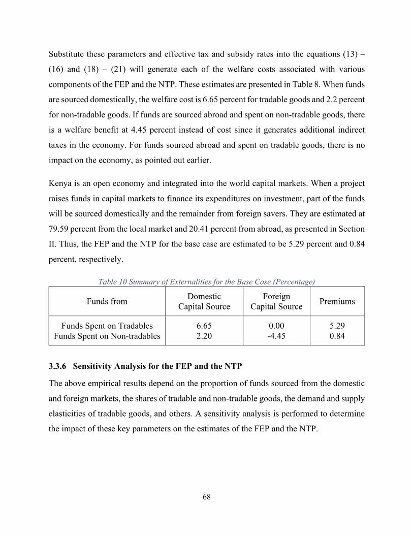
68
Substitute these parameters and effective tax and subsidy rates into the equations (13) –
(16) and (18) – (21) will generate each of the welfare costs associated with various
components of the FEP and the NTP. These estimates are presented in Table 8. When funds
are sourced domestically, the welfare cost is 6.65 percent for tradable goods and 2.2 percent
for non-tradable goods. If funds are sourced abroad and spent on non-tradable goods, there
is a welfare benefit at 4.45 percent instead of cost since it generates additional indirect
taxes in the economy. For funds sourced abroad and spent on tradable goods, there is no
impact on the economy, as pointed out earlier.
Kenya is an open economy and integrated into the world capital markets. When a project
raises funds in capital markets to finance its expenditures on investment, part of the funds
will be sourced domestically and the remainder from foreign savers. They are estimated at
79.59 percent from the local market and 20.41 percent from abroad, as presented in Section
II. Thus, the FEP and the NTP for the base case are estimated to be 5.29 percent and 0.84
percent, respectively.
Table 10 Summary of Externalities for the Base Case (Percentage)
Funds from Domestic
Capital Source
Foreign
Capital Source Premiums
Funds Spent on Tradables
Funds Spent on Non-tradables
6.65
2.20
0.00
-4.45
5.29
0.84
3.3.6 Sensitivity Analysis for the FEP and the NTP
The above empirical results depend on the proportion of funds sourced from the domestic
and foreign markets, the shares of tradable and non-tradable goods, the demand and supply
elasticities of tradable goods, and others. A sensitivity analysis is performed to determine
the impact of these key parameters on the estimates of the FEP and the NTP.
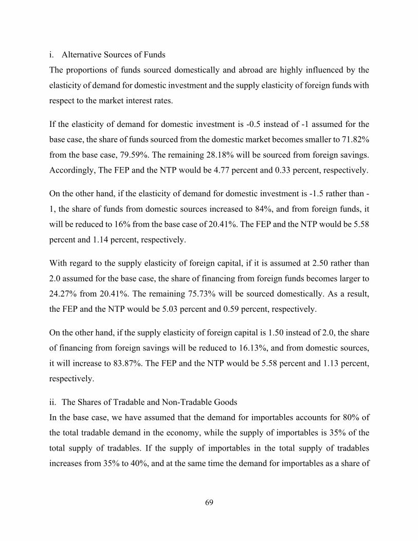
69
i. Alternative Sources of Funds
The proportions of funds sourced domestically and abroad are highly influenced by the
elasticity of demand for domestic investment and the supply elasticity of foreign funds with
respect to the market interest rates.
If the elasticity of demand for domestic investment is -0.5 instead of -1 assumed for the
base case, the share of funds sourced from the domestic market becomes smaller to 71.82%
from the base case, 79.59%. The remaining 28.18% will be sourced from foreign savings.
Accordingly, The FEP and the NTP would be 4.77 percent and 0.33 percent, respectively.
On the other hand, if the elasticity of demand for domestic investment is -1.5 rather than -
1, the share of funds from domestic sources increased to 84%, and from foreign funds, it
will be reduced to 16% from the base case of 20.41%. The FEP and the NTP would be 5.58
percent and 1.14 percent, respectively.
With regard to the supply elasticity of foreign capital, if it is assumed at 2.50 rather than
2.0 assumed for the base case, the share of financing from foreign funds becomes larger to
24.27% from 20.41%. The remaining 75.73% will be sourced domestically. As a result,
the FEP and the NTP would be 5.03 percent and 0.59 percent, respectively.
On the other hand, if the supply elasticity of foreign capital is 1.50 instead of 2.0, the share
of financing from foreign savings will be reduced to 16.13%, and from domestic sources,
it will increase to 83.87%. The FEP and the NTP would be 5.58 percent and 1.13 percent,
respectively.
ii. The Shares of Tradable and Non-Tradable Goods
In the base case, we have assumed that the demand for importables accounts for 80% of
the total tradable demand in the economy, while the supply of importables is 35% of the
total supply of tradables. If the supply of importables in the total supply of tradables
increases from 35% to 40%, and at the same time the demand for importables as a share of
70
total demand for tradables is assumed to be 70% instead of 80%, the results indicate that
the FEP and the NTP would be 4.95% and 1.81%, respectively.
iii. Compensated Own Price Elasticity Demand for Imports
If the compensated own-price elasticity of demand for imports will become -1.80 rather
than -1.52 for the base case. In this situation, the FEP would be 5.49%; for the NTP, the
premium would be 0.30%. On the other hand, if the compensated own-price elasticity of
demand for imports becomes -1.20, the FEP would be 5.08%; for the NTP, the premium
would be 1.45%.
The results of the sensitivity analysis are summarized in Table 9. The value of the FEP
ranges from 4.77% to 5.58% of the market value on tradable goods. For the NTP, it ranges
from 0.30% to 1.81% of the market value on non-tradable goods. Hence, the average values
of all extreme cases of the FEP and NTP are 5.21% and 0.96%, respectively.
Table 11 Results of Sensitivity Analysis for the FEP and NTP for Kenya
Scenarios Key Assumptions FEP NTP
Base Case
- Sources of Funds: Domestic: 81.84%, Foreign: 18.16%.,
(With ef = 2.0 & h = -1.0)
- Demand and supply of importables in total tradables: 80% and 35%. - Compensated Own Price Elasticity
Demand for Imports: -1.515
5.29% 0.84%
Sensitivity Analysis:
Sources of Funds
§ Due to change in elasticity
of demand for domestic
investment (h is -0.5 & -1.5
in lower & upper bounds)
Domestic: 71.82%, Foreign: 28.18% 4.77% 0.33%
Domestic: 84%, Foreign: 16% 5.58% 1.14%

71
§ Due to change in supply
elasticity of foreign savings
(ef is 1.50 & 2.50 in lower &
upper bounds)
Domestic 83.87%: Foreign: 16.13% 5.58% 1.13%
Domestic: 75.73%, Foreign: 24.27% 5.03% 0.59%
Demand and supply of importables in total tradables
Demand: 70%, Supply: 40% 4.95% 1.81%
Compensated Own Price Elasticity Demand for Imports
-1.80 5.49% 0.30%
-1.20 5.08% 1.45%
Although more cases could be simulated, we believe that a value of 5.2% for the FEP and
1.0% for the NTP would be the reasonable estimates for augmenting the financial values
of tradable and non-tradable goods in the financial cash flow statement to the economic
values in the economic resource statement while conducting the economic evaluation of
investment projects in Kenya.
4. Concluding Remarks
This paper has described the analytical framework and the practical approach to the
estimation of the economic opportunity cost of capital and the premiums on the foreign
exchange and non-tradable outlays for Kenya. These national economic parameters are the
key variables in estimating the net economic costs and benefits of investment projects.
The approach used to measure the economic opportunity cost of capital in this study is the
weighted average approach. This approach considers the opportunity cost of raising funds
in the capital markets for use in an investment project. Since the resources to be used in
investment projects are limited, the rate of return to a proposed investment must be
compared with the weighted average of the forgone returns that would have been generated
by the ultimate sources of these funds. An increase in the demand for investable funds
drives the market interest rate up. Consequently, some reproducible remunerative capital
investment would be displaced, and the domestic and foreign savings would be stimulated.
72
Employing this method, we estimate that the real economic opportunity cost of capital
would be approximately 11.36 percent in the base case.
Given the data obtained for the analysis and to ensure the robustness of the estimated
values, we performed a sensitivity analysis by allowing the key parameters that have an
impact on the measurement of the economic discount rate. The results suggest that
estimates of the discount rate can range from 9.91 percent to 12.70 percent real.
Consequently, we recommend that an 11.5 percent rate is an appropriate discount rate to
use when calculating the economic net present value of the flows of economic benefits and
costs over time.
The other national parameter is the foreign exchange premium, and the premium for non-
tradable outplays. They are important for converting all financial cash flows into the
economic resource statement in a consistent manner. This is due to the fact that various
indirect tax and subsidy distortions are contemporarily affecting the financial value of
tradable and non-tradable goods. Given the resource constraints, the analysis is undertaken
in a general equilibrium in which resources must be shifted between tradable and non-
tradable sectors in response to the relative price between these two sectors. The tax and
other distortions must be measured in order to capture their impacts on the economy. The
empirical results suggest that the economic value of the foreign exchange (FEP) exceeds
the market exchange rate by 5.2 percent, and the shadow price of non-tradable goods and
services (NTP) is just 1.0% higher than their financial values. These premiums need to be
incorporated in the economic evaluation of investment projects.
The estimation of national parameters for Kenya has been a challenge with respect to data
availability. In spite of this challenge, the methodology employed in this report is sound
and the empirical simulations with various sensitivity analyses present robust estimates for
the social discount rate and the premiums on the foreign exchange and non-tradable outlays
to be used for economic appraisals of both public and private investment projects in Kenya.

73
References
Agénor, P.-R., & Moreno-Dodson, B. (2006). Public Infrastructure and Growth: New Channels
and Policy Implications. World Bank.
Aschauer, D. A. (1989). Is public expenditure productive? Journal of Monetary Economics, 23(2),
177–200.
Baumol, W. (1968). On the social rate of discount. The American Economic Review, 788–802.
Boadway, R. (1978). Public investment decision rules in a neo-classical growing Economy.
International Economic Review, 265–287.
Bradford, D. F. (1975). Constraints on Government Investment Opportunities and the Choice of
Discount Rate. In The American Economic Review (Vol. 65, Issue 5).
Burgess, D. F. (1988). Complementarity and the Discount Rate for Public Investment. In The
Quarterly Journal of Economics (Vol. 103, Issue 3).
Burgess, D. F., & Zerbe, R. O. (2013). The most appropriate discount rate. Journal of Benefit-Cost
Analysis, 4(03), 391–400.
Central Bank of Kenya. (2021). Dataset.
Coppola, A., Fernholz, F., & Glenday, G. (2014). Estimating the Economic Opportunity Cost of
Capital for Public Investment Projects an Empirical Analysis of the Mexican Case. World
Bank Policy Research Working Paper, (6816).
Damodaran, A. (2019). Country Risk: Determinants, Measures and Implications The 2019 Edition.
SSRN Electronic Journal.
Diamond, P. A., & Mirrlees, J. A. (1971). Optimal Taxation and Public Production I: Production
Efficiency. In the American economic review (Vol. 61, Issue 1).
East African Community. (2017). Common External Tariff 2017 Version.

74
Edwards, S. (1986). Country risk, foreign borrowing, and the social discount rate in an open
developing economy. Journal of International Money and Finance, S79–S96.
Excise Duty Act, 2015, 181 1710 (2015).
Feenstra, R. C., Inklaar, R., & Timmer, M. P. (2015). The next generation of the penn world table.
American Economic Review, 105(10), 3150–3182.
Feldstein, M. (1964). The social time preference discount rate in cost-benefit analysis. The
Economic Journal, 74(294), 360–379.
Gollin, D. (2002). Getting income shares right. Journal of Political Economy, 110(2), 458–474.
Gomis, R. (2019). The global labor income share and distribution. ILO Department of Statistics,
Methodological Description. Geneva, ILO.
Gueye, C., & Sy, A. (2015). Beyond aid: how much should African countries pay to borrow?
Journal of African Economies, 352–366.
Hagen, K. (1983). Optimal shadow prices and discount rates for budget-constrained public firms.
Journal of Public Economics, 22(1), 27–48.
Harberger, A. C., & Jenkins, G. P. (2002). Readings in Economic Cost-Benefit Analysis. Cost-
Benefit Analysis, Northampton MA: Edward Elgar Publishers, Ltd.
Harberger, A. (1988). Perspectives on capital and technology in less-developed countries. Estudios
de Economía (Chile).
Harberger, A. (1969). On measuring the social opportunity cost of public funds, in Proceedings of
the Committee on Water Resources and Economic Development of the West. 1–24.
Harberger, A. C., Jenkins, G. P., & Jenkins Musings, G. P. (2015). Musings on the Social Discount
Rate. Journal of Benefit-Cost Analysis, 6(1), 6–32.
Harberger, A. C., & Wisecarver, D. L. (1977). Private and Social Rates of Return to Capital in
Uruguay. In Source: Economic Development and Cultural Change (Vol. 25, Issue 3).

75
Hoffmann, E. (2003). International Classification of Status in Employment, ICSE-93. In Advances
in Cross-National Comparison (pp. 125–136). Springer US.
International Labour Organization. (2021). International Labour Organization, ILOSTAT
database. Data were retrieved on April 25, 2021.
International Monetary Fund. (2021). World Economic Outlook Databases. World Economic
Outlook (WEO).
International Monetary Fund. (2021). International Monetary Fund. Investment and Capital
Dataset (ICSD).
International Monetary Fund. (2021). Government Finance Dataset.
International Monetary Fund. African Dept. (2021). Kenya: Requests for an Extended
Arrangement Under the Extended Fund Facility and an Arrangement Under the Extended
Credit Facility-Press Release; Staff Report; and Statement by the Executive Director for
Kenya.
Jenkins, G., Kuo, C., & Harberger, A. (2019). Cost-Benefit Analysis for Investment Decisions
Chapters 8 and 9.
Jenkins, G., & Kuo, C. (2007). The economic opportunity cost of capital for Canada- an empirical
update. (No. 1133). Queen’s Economics Department Working Paper.
Jenkins, G., & Kuo, C. (1998). Estimation of the National Parameters for Economic Cost-Benefit
Analysis for the Philippines.
Kee Hiau, L., Nicita, A., & Olarreaga, M. (2008). Import demand elasticities and trade distortions.
Review of Economics and Statistics, 90(4), 666–682.
Kenya Institute for Public Policy Research and Analysis. (2019). Kenya Economic Report (2019):
Resource Mobilization for Sustainable Development of Kenya.
Kenya Institute for Public Policy Research and Analysis. (2020). Kenya Economic Report (2020):
Creating an Enabling Environment for Inclusive Growth in Kenya.
76
Kenya National Bureau of Statistics. (2019). Statistical Abstract, 2019.
Kenya National Bureau of Statistics. (2015). Statistical Abstract, 2015.
Kenya National Bureau of Statistics. (2014). Statistical abstract 2014.
Kenya National Bureau of Statistics. (2010). Statistical Abstract 2010.
Kuo, C.-Y., Jenkins, G. P., & Mphahlele, B. (2003). The Economic Opportunity Cost of Capital
for South Africa. The South African Journal of Economics, 71, 496–516.
Kuo, C.-Y., Salci, S., & Jenkins, G. P. (2015). Measuring the Foreign Exchange Premium and the
Premium for Non‐Tradable Outlays for 20 Countries in Africa. South African Journal of
Economics, 83(2), 269–285.
Lind, R. (1982). A primer on the major issues relating to the discount rate for evaluating national
energy options. Discounting for Time and Risk in Energy Policy.
Marchand, M., & Pestieau, P. (1984). Discount rates and shadow prices for public investment.
Journal of Public Economics, 24(2), 153–169.
Marglin, S. (1963). The opportunity costs of public investment. The Quarterly Journal of
Economics, 274–289.
Medina, L., Jonelis, M., & Cangul, M. (2017). The informal economy in Sub-Saharan Africa: Size
and determinants. International Monetary Fund.
Mishan, E. J. (1967). Criteria for Public Investment: Some Simplifying Suggestions. Journal of
Political Economy, 75(2), 139–146.
Ogaki, M., Ostry, J. D., & Reinhart, C. M. (1996). Saving behavior in low- and middle-income
developing countries a comparison. IMF Staff Papers, 43(1), 38–71.
Othman, A., & Jenkins, G. P. (2020). Estimation of the rate of return to capital in the East African
Community (EAC) Countries. Applied Economics, 52(30), 3257–3273.

77
Poterba, J. (1998). The rate of return to corporate capital and factor shares: New estimates using
revised national income accounts and capital stock data—Carnegie-Rochester Conference
Series on Public Policy.
Ramsey, D. (1969). On the social rate of discount: Comment. The American Economic Review,
59(5), 919–924.
Robles, E. (1998). An exploration into the sources and causes of economic growth in the United
States and fourteen Latin American countries.
Sandmo, A., & Drèze, J. H. (1971). Discount Rates for Public Investment in Closed and Open
Economies. In Economica (Vol. 38, Issue 152).
Sen, A. (1961). On optimizing the rate of saving. The Economic Journal, 71,(283), 479–496.
Sjaastad, L. A., & Wisecarver, D. L. (1977). The Social Cost of Public Finance. Journal of
Political Economy, 85(3), 513–547.
The Ministry of Planning and Devolution. (2007). The Kenya Vision 2030. In Government of the
Republic of Kenya.
Tokarick, S. (2014). A method for calculating export supply and import demand elasticities A
method for calculating export supply and import demand elasticities. The Journal of
International Trade & Economic Development, 23(7), 1059–1087.
UNCTAD, S. (2021). UNCTAD STAT.
Usher, D. (1969). On the social rate of discount: Comment. The American Economic Review,
59(5), 925–929.
Value Added Tax Act No. 35 of 2013.
World Bank. (2021). International Debt Statistics.
World Bank. (2021). World development indicators. Data were retrieved on June 10, 2021.

Appendix A. Return to Domestic Investment in Kenya 2006-2019 (Million Ksh)
Current Prices (Million KSh)
Year GDP Compensation of employees
LIS (%GDP)
Total Labor
Income
Taxes on
Products VAT
Subsidies on
Products GVA by
AGR
GVA of Mining
and quarrying
Resource Rents
Capital’s share of
Intermediation Cost
Economic Dep.Expense
Gross-of-tax
Return to Capital
GDP Deflator
Index (2009=1)
Real Return to Capital (2009 prices)
Reproducible Capital Stock
Remunerative capital stock
Real Value of Remunerative capital stock (2009 prices)
Real Rate of Return to
Remunerative Capital
(1) (2) (3) (4) (5) (6) (7) (8) (9) (10) (11) (12) (13) (14) (15) (16) (17) (18) (19)
2006 1,862,384 665,048 46% 856,697 91,571 79,926 421 350,737
10,028 351 2,105 255,710 509,956 0.72 708,853 5,095,264 3,719,543 5,170,268 13.71%
2007 2,151,615 752,482 45% 970,378 116,346 96,497 45 405,525
13,771 482 2,130 289,379 606,478 0.78 779,635 5,720,936 4,176,283 5,368,663 14.52%
2008 2,483,264 854,877 42% 1,030,554 126,594 111,905 72 510,355
16,786 588 3,002 295,607 820,697 0.90 916,201 6,795,266 4,960,544 5,537,805 16.54%
2009 2,863,795 925,268 42% 1,214,249 143,047 126,854 94 618,724
18,134 635 5,441 332,780 919,060 1.00 919,060 7,815,800 5,705,534 5,705,534 16.11%
2010 3,170,687 1,006,579 45% 1,420,468 158,372 148,353 107 730,394
26,029 911 6,397 364,763 917,873 1.02 899,047 8,308,541 6,065,235 5,940,834 15.13%
2011 3,727,416 1,123,816 43% 1,610,244 175,372 171,881 18,207 912,529
32,514 1,138 15,392 422,527 1,139,681 1.13 1,007,577 9,601,051 7,008,767 6,196,362 16.26%
2012 4,261,370 1,247,283 44% 1,866,480 182,245 176,386 32,027 1,028,364
46,628 1,632 18,245 475,466 1,321,976 1.24 1,068,514 10,991,953 8,024,126 6,485,662 16.48%
2013 4,745,090 1,452,179 45% 2,125,800 196,634 184,916 22,475 1,153,215
40,742 1,426 19,866 561,868 1,394,966 1.30 1,072,094 12,082,117 8,819,945 6,778,525 15.82%
2014 5,402,647 1,691,612 46% 2,463,607 253,037 232,630 30,584 1,372,197
44,936 1,573 22,595 730,422 1,400,248 1.41 995,810 13,779,501 10,059,036 7,153,652 13.92%
2015 6,284,185 1,881,911 44% 2,771,326 241,284 259,685 30,324 1,777,350
54,584 1,910 19,390 815,724 1,740,169 1.55 1,124,794 15,921,801 11,622,914 7,512,710 14.97%
2016 7,022,963 2,014,137 42% 2,942,622 267,027 289,213 29,970 2,055,465
59,149 2,070 22,310 861,022 2,132,951 1.63 1,306,171 17,382,012 12,688,869 7,770,376 16.81%
2017 8,165,842 2,371,295 44% 3,584,805 301,862 339,034 55,477 2,706,786
61,225 2,143 29,802 1,186,697 2,028,727 1.81 1,119,817 20,021,774 14,615,895 8,067,681 13.88%
2018 8,892,111 2,586,544 44% 3,908,325 311,890 356,856 60,279 2,873,516
67,648 2,368 29,765 1,318,020 2,225,217 1.86 1,199,222 21,244,516 15,508,497 8,357,897 14.35%
2019 9,740,360 2,830,810 44% 4,261,216 390,832 435,886 61,651 3,151,842
67,330 2,357 31,725 1,491,596 2,341,172 1.93 1,213,640 22,864,786 16,691,294 8,652,598 14.03%
Average 15.18% Sources & Notes: Columns (1), (2), (8), (9), (12) are obtained from the national accounts data, Kenya National Bureau of Statistics.
Column (3) is obtained from the ILO dataset.
Column (4) = (1) * (3)
Columns (5), (6), (7) are obtained from Statistical Abstract, Kenya National Bureau of Statistics, Nairobi
Column (10) = (9) * 3.5%
Column (11) is calculated as half of (6%*GFCF_private sector).
Column (13) = (1) – (4) – ((5)*(3)) – (6) + ((7)*(1-(3)) – ((8)*33%) – (10) – (11) – (12)
Column (14) is obtained from World Bank, national accounts data.
Column (15) = (13)/ (14)
Column (16) is obtained from appendix B.
Column (17) = (16) * 73%
Column (18) = (17) / (14)
Column (19) = (15) / (18)
Abbreviations: LIS: Labor Income Share; GVA: Gross Value Added; AGR: Agriculture.
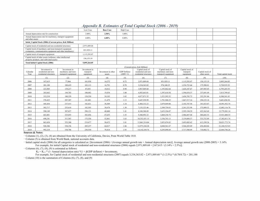
Appendix B. Estimates of Total Capital Stock (2006 - 2019) Low Case Base Case High Case Annual depreciation rate for construction 2.00% 2.50% 3.00% Annual depreciation rate for machinery, transport equipment and other assets
4.00% 6.00% 8.00%
Intial_Capital Stock (2006) (Current prices, Ksh Million) Capital stock of residential and non-residential structures 2,971,889.68 Capital stock of machinery and (non-transport) equipment (computers, communication equipment and other machinery)
851,929.11
Capital stock of transport equipment 1,115,292.07 Capital stock of other assets (software, other intellectual property products, and cultivated assets)
156,153.19
Total Initial Capital Stock (2006) 5,095,264.05 (Current prices, Ksh Million) Calendar
Year
Investment in residential and non-residential structures
Investment in machinery and (non-transport) equipment
Investment in transport
equipment Investment in other
assets GDP Deflator
(2009 =1)
Capital stock of residential and non-residential structures
Capital stock of machinery and (non-transport) equipment
Capital stock of transport
equipment Capital stock of
other assets Total capital stock
(1) (2) (3) (4) (5) (6) (7) (8) (9) (10)
2006 167,615 77,866 101,938 14,272 0.72 2,971,889.68 851,929.11 1,115,292.07 156,153.19 5,095,264.05
2007 201,188 108,419 103,113 16,791 0.78 3,334,363.02 974,340.25 1,236,723.44 175,508.81 5,720,935.52
2008 223,505 139,217 87,693 18,012 0.90 3,967,069.60 1,193,862.64 1,426,347.47 207,985.85 6,795,265.55
2009 265,662 144,785 100,042 19,434 1.00 4,583,663.01 1,397,610.58 1,596,834.37 237,691.69 7,815,799.65
2010 315,218 180,329 124,330 24,183 1.02 4,877,871.32 1,521,592.52 1,656,785.73 252,291.86 8,308,541.43
2011 378,422 207,307 141,881 31,479 1.13 5,647,559.99 1,791,948.25 1,867,317.16 294,225.18 9,601,050.58
2012 445,454 237,415 182,821 38,509 1.24 6,468,332.22 2,079,849.08 2,102,747.58 341,023.87 10,991,952.74
2013 502,717 253,618 182,503 38,678 1.30 7,135,323.46 2,309,730.83 2,261,252.98 375,809.52 12,082,116.78
2014 590,149 307,037 298,121 40,800 1.41 8,108,388.09 2,653,356.07 2,595,194.29 422,562.69 13,779,501.14
2015 682,801 325,055 302,856 47,655 1.55 9,380,992.22 3,069,238.75 2,986,887.04 484,682.53 15,921,800.53
2016 698,241 311,507 175,556 52,861 1.63 10,352,431.15 3,356,743.13 3,139,084.57 533,752.89 17,382,011.74
2017 863,454 353,280 219,477 56,673 1.81 12,061,514.04 3,853,874.83 3,493,085.62 613,299.26 20,021,773.74
2018 928,306 338,156 205,237 64,017 1.86 12,973,184.20 4,048,561.67 3,568,285.09 654,484.86 21,244,515.83
2019 992,218 338,706 230,530 70,418 1.93 14,142,104.76 4,295,098.69 3,717,580.09 710,002.72 22,864,786.26
Sources & Notes: - Columns (1), (2), (3), (4) are obtained from the University of California, Davies, Penn World Table 10.0.
- Column (5) is obtained from World Bank, national accounts data.
- Initial capital stock (2006) for all categories is calculated as: [Investment (2006) / (Average annual growth rate + Annual depreciation rate)]. Average annual growth rate (2000-2005) = 3.14%
For example, for initial Capital stock of residential and non-residential structures (2006) equals 2,971,889.68 = [167,615 / (3.14% + 2.5%)].
- Columns (6), (7), (8), (9) is estimated as follows:
Kti = Kti-1 * (1- Annual depreciation rate) *(1 + ∆GDP deflator) + Investmentti
For example, for Capital stock of residential and non-residential structures (2007) equals 3,334,363.02 = 2,971,889.68 * (1-2.5%) * (0.78/0.72) + 201,188
- Column (10) is the summation of Columns (6), (7), (8), and (9)
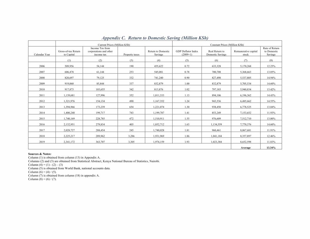
Appendix C. Return to Domestic Saving (Million KSh) Current Prices (Million KSh) Constant Prices (Million KSh)
Calendar Year Gross-of-tax Return
to Capital
Income Tax from corporations and other
income tax Property taxes Return to Domestic
Savings GDP Deflator Index
(2009=1) Real Return to
Domestic Savings Remunerative capital
stock
Rate of Return to Domestic
Savings
(1) (2) (3) (4) (5) (6) (7) (8)
2006 509,956 54,144 190 455,622 0.72 633,328 5,170,268 12.25%
2007 606,478 61,144 253 545,081 0.78 700,708 5,368,663 13.05%
2008 820,697 79,125 332 741,240 0.90 827,498 5,537,805 14.94%
2009 919,060 85,844 337 832,879 1.00 832,879 5,705,534 14.60%
2010 917,873 103,655 342 813,876 1.02 797,183 5,940,834 13.42%
2011 1,139,681 127,996 352 1,011,333 1.13 894,106 6,196,362 14.43%
2012 1,321,976 154,134 490 1,167,352 1.24 943,536 6,485,662 14.55%
2013 1,394,966 173,239 654 1,221,074 1.30 938,450 6,778,525 13.84%
2014 1,400,248 199,717 743 1,199,787 1.41 853,249 7,153,652 11.93%
2015 1,740,169 228,785 472 1,510,911 1.55 976,609 7,512,710 13.00%
2016 2,132,951 279,834 405 1,852,712 1.63 1,134,559 7,770,376 14.60%
2017 2,028,727 288,454 245 1,740,028 1.81 960,461 8,067,681 11.91%
2018 2,225,217 289,962 3,286 1,931,969 1.86 1,041,184 8,357,897 12.46%
2019 2,341,172 363,707 3,305 1,974,159 1.93 1,023,384 8,652,598 11.83%
Average 13.34%
Sources & Notes: Column (1) is obtained from column (13) in Appendix A.
Columns (2) and (3) are obtained from Statistical Abstract, Kenya National Bureau of Statistics, Nairobi.
Column (4) = (1) - (2) – (3)
Column (5) is obtained from World Bank, national accounts data.
Column (6) = (4) / (5).
Column (7) is obtained from column (18) in appendix A.
Column (8) = (6) / (7).

Appendix D. Share of Foreign Savings in Total Private-Sector Savings (Current prices, millions USD,) (2009 prices, Millions KSh)
Year External Long-term
Debt Stock Foreign Direct Investment
(FDI) Stock, Inward Total Long-term debt
and FDI Stock
Official exchange rate (LCU per US$, period
average)
Total Long-term debt and FDI Stock (Current prices) (Millions KSh)
GDP Deflator Index (2009=1)
Total Long-term debt and FDI Stock
Total reproducible capital stock
Share of Foreign Investment to the total
reproducible capital stock
(1) (2) (3) (4) (5) (6) (7) (8) (9)
2006 5,893 1,164 7,057 72 508,492 0.72 706,818 7,082,559 9.98%
2007 6,254 2,272 8,526 67 573,807 0.78 737,636 7,354,333 10.03%
2008 6,410 2,760 9,170 69 634,555 0.90 708,399 7,586,034 9.34%
2009 6,741 4,251 10,992 77 848,987 1.00 848,987 7,815,800 10.86%
2010 6,998 5,449 12,447 79 985,406 1.02 965,195 8,138,129 11.86%
2011 7,764 6,899 14,663 89 1,302,096 1.13 1,151,167 8,488,167 13.56%
2012 9,004 8,279 17,283 84 1,459,903 1.24 1,179,996 8,884,468 13.28%
2013 9,908 9,398 19,306 86 1,662,433 1.30 1,277,655 9,285,650 13.76%
2014 13,587 10,219 23,806 88 2,093,667 1.41 1,488,946 9,799,523 15.19%
2015 15,874 10,839 26,713 98 2,622,982 1.55 1,695,419 10,291,384 16.47%
2016 17,824 11,518 29,341 102 2,979,155 1.63 1,824,367 10,644,351 17.14%
2017 22,494 12,784 35,278 103 3,648,158 1.81 2,013,710 11,051,618 18.22%
2018 27,263 14,410 41,673 101 4,220,362 1.86 2,274,453 11,449,175 19.87%
2019 30,886 15,742 46,628 102 4,756,404 1.93 2,465,672 11,852,874 20.80%
Average 14.31% Sources & Notes: Column (1) is obtained from World Bank, International Debt Statistics.
Column (2) is obtained from UNCTADSTAT.
Column (3) = (1) + (2)
Column (4) is obtained from WB, World Bank Global Economic Monitor.
Column (5) = (3) * (4)
Column (6) is obtained from World Bank, National Accounts Data.
Column (7) = (5) / (6)
Column (8) is the real value of column (10) in Appendix B.
Column (9) = (7) / (8).

[This page is intentionally left blank]
83
Annexure B: Estimation of Commodity-Specific Conversion
Factors Report
Estimation of National Parameters and Commodity Specific Conversion Factors (CSCFs) Estimation of CSCFs for Tradable and Non-tradable Commodities Date: July 28, 2021 Submitted by: Cambridge Resources International, Inc. 1770Mass.Ave#617,Cambridge,MA02140,USA Phone: 1 (613) 770 2080 E-mail: [email protected] or [email protected]
In Consortium with: GEEKAN KENYA LTD RUPRANI HOUSE, MOKTAR DADAH P.O BOX 17460-00100 TEL:+254723729096 Email: [email protected] NAIROBI-KENYA. Presented to: THE MINISTRY OF NATIONAL TREASURY AND PLANNING, KENYA

85
Estimation of Commodity-Specific Conversion Factors for the Republic of Kenya
The Commodity-Specific Conversion Factors (CSCF) Database55 has been developed for the Republic of Kenya. CSCFs are used to translate market prices for goods and services into corresponding economic value by accounting for various distortions that are present in the Kenyan economy such as taxes, subsidies, monopolies, etc. The database contains CSCFs for all tradable commodities (5,679), listed under the Harmonized System for classifying goods, and 14 non-tradable items (i.e., Administration, Communication, Construction, Education, Electricity, Extension services, Finance, Health, Hotels, Other services, Real estate, Trade, Transport, and Water).
The report is organized in three chapters. The first chapter briefly explains and presents the toolkit prepared for Kenya. Second section presents the methodology and estimation results for tradable commodities while the last section presents the same for non-tradable commodities and services.
1. CSCF Toolkit
Kenya CSCF Database is a web-based software that provides open access to the national parameters and CSCFs for tradable and non-tradable commodities and services. The program provides multiple ways to search and browse the database with an easy-to-learn interface. It is designed for professionals, policy makers, and academia involved in the economic and social appraisal of public investment projects in Kenya.
1.1. Website In-brief
Users will be met with a homepage every time they visit the website. All sections of the website can be accessed using the top navigation panel (i.e., tradable conversion factors, non-tradable conversion factors, national parameters and help).
For non-tradable conversion factors, users can estimate conversion factors for 14 non-tradables through a drop-down list. For tradable commodities, the website is equipped with a search engine that facilitates searching for the tradable commodities in the database. Users can search according to a keyword, HS Code, or (Sub)Chapter Number.
Website is also equipped with a feature that allow users to browse tradable commodities by categories. The Browse Categories page provides an alternative way to search through tradable commodities, categorized into 99 HS chapters. When a user selects a chapter, the chapter will expand and reveal all sub-chapters associated with the chapter. Once the sub-chapter is also selected, it will expand to show all commodities within the sub-chapter. For each commodity
55 The database is accessible through http://kenya.cri-world.com .

86
selected, four different types can be selected to reveal different estimations, which are “Importable Input”, “Importable Output”, “Exportable Input” and “Exportable Output”.
Users are allowed to automatically save their estimation results to an excel file. Users can add various commodities (tradable or non-tradable) or different types of a particular tradable commodity to the download list each time CSCF is displayed for the commodity. Once the desired numbers of items are added to the list, the list can be downloaded for their future reference.
The website is designed in a manner that allow users to update key inputs of each tradable commodity or non-tradable service to the website temporarily. For instance, the estimates of CSCFs for tradable goods can be easily updated if either the custom duty rates, value-added taxes, environmental tax, or FEP changes. Temporary changes of the inputs only affect each specific user and will automatically reverts to its default value as the user surfs through the website. Maintenance of the website and permanent update of the key inputs is only restricted to the users with administrative access to the website through administrator login credentials and will change the results for all different users permanently.
Here below you may find snapshots of the toolkit.
Figure 3: Homepage

87
Figure 4: Searching Tradable Commodities
Figure 5: Browsing Tradables by Category
Figure 6: Non-tradable drop-down list
Figure 7: National Parameters for Kenya
2. Conversion Factors for Tradables
2.1. Methodology
A good or service is considered tradable when an increase in demand (supply) by a project does not affect the amount demanded (supplied) by domestic consumers (producers). The increase in demand (supply) by a project is eventually reflected as an increase (decrease) in imports or a

88
decrease (increase) in exports depending on whether the project is demanding or supplying the importable or exportable commodity.
Kenya importable goods include (a) all goods imported into Kenya and (b) all goods produced and sold domestically that are close substitutes for either the imported goods or potentially imported goods. Kenya exportable goods, on the other hand, include (a) all goods exported by Kenya and (b) domestic consumption of similar or close substitutes for the exported goods.
The first step in estimating CSCFs for tradable commodities is to determine the applicable tax rates for each commodity using the latest Harmonized Commodity Description and Coding System. Next, the corresponding distortions are identified and applied. These distortions include import tariffs, export taxes, subsidies, value added tax (VAT), other indirect taxes and non-tariff barriers such as quotas. The distortions will have a considerable influence on the financial prices of the goods in the market. From the economic point of view, however, it is the world price that reflects the value of the good. Taxes are resource transfers from consumers to the Kenyan Government. Lastly, depending on whether the commodity is an input for or the output of the project, the CSCF is calculated according to the following formulae.56
Importable inputs/outputs: !"!#!!&!$
=1 + #'(
1 + )% − +% + ()& + )') × (1 + )% − +%) + /0# + 102 + 34) × (1 + )% − +% + )&(1 + )% − +%) + )'(1 + )% − +%))
Where, • FEP is the foreign exchange premium. • !! stands for the rate of import duty levied on the CIF price of the imported input • "! is the rate of import subsidy expressed as the percentage of the CIF price • !" is the rate of excise duty levied on the CIF price plus the import duty on the imported input (retail price excluding VAT) • !# is the rate of Road Maintenance Levy (RML), Petroleum Regulation Levy (PRL), and Petroleum Development Levy (PDL).
This applies on the CIF price plus the import duty/subsidy on the imported input (retail price excluding VAT). • #$% is Import Declaration Fee • &$' is Railway Development Levy • VAT is the value added tax rate levied on the basis of the sum of CIF price plus import duty, excise duty, RML, PRL, and
PDL. Exportable inputs/outputs:
!"!#56 =1 + #'(
1 + )7 − +7 + ,-+(1 + )7 − +7)!"!#58 =
1 + #'((1 + )7 − +7)
Where, • FEP is the foreign exchange premium • "$stands for the rate of export subsidy, (expressed as the percentage of the FOB price) • !$is the rate of export tax, (expressed as the percentage of the FOB price)
56 More detailed theoretical aspects of the economic prices of tradable commodities can be accessed from Jenkins et al. (2011), DDP 2011-10, John Deutsch International, Queen’s University, Canada. URL: http://ideas.repec.org/p/qed/dpaper/203.html
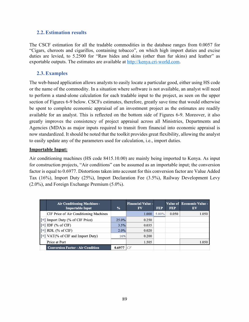
89
2.2. Estimation results
The CSCF estimation for all the tradable commodities in the database ranges from 0.0057 for “Cigars, cheroots and cigarillos, containing tobacco”, on which high import duties and excise duties are levied, to 5.2500 for “Raw hides and skins (other than fur skins) and leather” as exportable outputs. The estimates are available at http://kenya.cri-world.com.
2.3. Examples
The web-based application allows analysts to easily locate a particular good, either using HS code or the name of the commodity. In a situation where software is not available, an analyst will need to perform a stand-alone calculation for each tradable input to the project, as seen on the upper section of Figures 6-9 below. CSCFs estimates, therefore, greatly save time that would otherwise be spent to complete economic appraisal of an investment project as the estimates are readily available for an analyst. This is reflected on the bottom side of Figures 6-9. Moreover, it also greatly improves the consistency of project appraisal across all Ministries, Departments and Agencies (MDA)s as major inputs required to transit from financial into economic appraisal is now standardized. It should be noted that the toolkit provides great flexibility, allowing the analyst to easily update any of the parameters used for calculation, i.e., import duties.
Importable Input:
Air conditioning machines (HS code 8415.10.00) are mainly being imported to Kenya. As input for construction projects, “Air conditions” can be assumed as an importable input; the conversion factor is equal to 0.6977. Distortions taken into account for this conversion factor are Value Added Tax (16%), Import Duty (25%), Import Declaration Fee (3.5%), Railway Development Levy (2.0%), and Foreign Exchange Premium (5.0%).

90
Figure 8: Importable Input
Importable Output:
Petroleum Jelly (HS Code 2712.10.00) is an output of a chemical factory. Assuming that Kenya is mainly importing petroleum jelly, this product is considered as an importable output for this factory. Conversion Factor is equal to 0.6656 considering 16% VAT, 25% import duty, 5% excise duty, 3.5% import declaration fee, 2.0% railway development levy, and 5.0% FEP.
Figure 9: Importable Output
Exportable Input:
Interchangeable Tools can be a good example of an Exportable Input for a construction work in Kenya. Interchangeable tools are being used in construction works as an input, and at the same
0.6977
0.6656
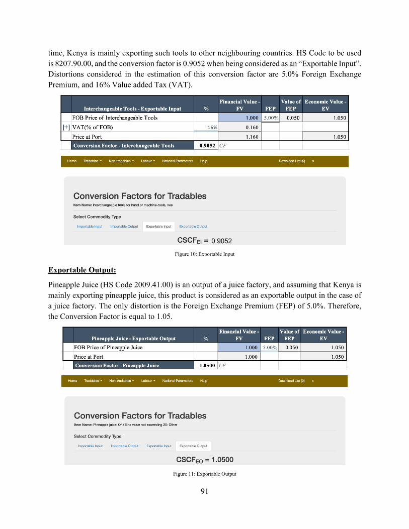
91
time, Kenya is mainly exporting such tools to other neighbouring countries. HS Code to be used is 8207.90.00, and the conversion factor is 0.9052 when being considered as an “Exportable Input”. Distortions considered in the estimation of this conversion factor are 5.0% Foreign Exchange Premium, and 16% Value added Tax (VAT).
Figure 10: Exportable Input
Exportable Output:
Pineapple Juice (HS Code 2009.41.00) is an output of a juice factory, and assuming that Kenya is mainly exporting pineapple juice, this product is considered as an exportable output in the case of a juice factory. The only distortion is the Foreign Exchange Premium (FEP) of 5.0%. Therefore, the Conversion Factor is equal to 1.05.
Figure 11: Exportable Output
0.9052

92
3. Conversion Factors for Non-tradables
The number of non-tradable goods and services in any economy is typically much smaller than that of tradable commodities. The database contains CSCFs for 14 non-tradable commodities. In contrast to tradable goods, the non-tradable services are only used as inputs into projects. In a situation when non-tradable service is an output of a project, i.e., roads, the value of this output is determined on a project-by-project basis.
3.1. Methodology
A good or service is considered non-tradable when its domestic price is determined by local demand and supply. An increase in demand (or supply) by a project could affect the amounts demanded by domestic consumers (or produced by other suppliers).
Conversion factors for non-tradable commodities is estimated by eliminating the distortions such as taxes, subsidies, trade taxes, licenses and quotas, monopoly mark-ups, environmental externalities, congestion costs, and any other type of price or quantity restriction that causes the demand price of the item to diverge from its supply price. A difference may exist between financial and economic prices, even in the absence of distortions.
In the case of the market for non-tradable commodities, increased demand for an input to be used by the project or increased supply of an output produced by the project would impact the market equilibrium price. This change will cause the other consumers and producers in the market to adjust their quantities consumed and produced, respectively. Additionally, in the presence of market distortions, other impacts are included in economic analysis.
To estimate the economic prices of non-tradable goods and services we first adjust for distortions in the market for the item itself. Second, we adjust for distortions in the market where demand is being diverted towards or away from. Third, distortions in the markets for the inputs used to produce the item are corrected. Correction is applied to the proportion of the item produced by other suppliers in the market. Finally, we apply a correction for the FEP and SPNTO on tradable and non-tradable components of the non-tradable good or service. This is done according to the following formula:57
(79 = 17:(7;(1 + )7) +17<(7;(1 + 27= − 3∗)
−17: 456?7@ (?
;3? +?
56A7@ (A
;3∗CD@
A
+56E7@ (E
;3E +E
56F7@ {1F<(F;(3∗ − 2F=)}F
9
+[(7; × +7 × #'(] + [(7; × =+7 × =+(]
!"!# =(79
(7; × (1 + 27
=)
57 Further theoretical details of the estimation of the economic prices of non-tradable goods and services can be found in Jenkins et al. (2011), DDP 2011-11, John Deutsch International, Queen’s University, Canada. URL: http://ideas.repec.org/p/qed/dpaper/204.html

93
where,
• Non-tradable output produced or purchased by the project • Economic price of output
• Supply weight for output
• Demand weight for output
• Market price per unit of output (net of value added tax, i.e., VAT)
• The rate of production subsidy on output
• VAT on output
• The overall effective tax rate on tradable and non-tradable goods and services in the economy
• !!"# ∶ Input-output coefficient for tradable input used in the production of a unit of output • Market price per unit of input (net of VAT)
• The rate of non-creditable tax or subsidy on the tradable inputs used in the production of output
• !$"# : Input-output coefficient for tradable input # used in the production of non-tradable inputs (direct tradable inputs to the NT inputs and the indirect tradable inputs of their subsequent inputs) used for a production of a unit of output
• $$% : Market price per unit of # • %∗()#: The overall average effective tax rate of the tradable inputs (in the whole economy) used
indirectly in the non-tradable inputs for a production of output excluding VAT. • !*"# : Input-output coefficient for direct and indirect labor input ' used in the production of a unit of
output • $*% : Market price per unit of labor ' • %* : The rate of distortions on the labor inputs used in the production of output • !+"# ∶Input-output coefficient for non-tradable input ) (direct input) used in the production of a unit of
output • *+, ∶ Demand weight for input ) • $+% ∶Market price per unit of input ) (net of VAT and distortions on tradable components of input )) • ++- ∶VAT on input ) paid by the new consumers of ) • Share of tradable components for output
• Share of non-tradable (i.e., Labor) components of output
• Foreign exchange premium • Premium on non-tradable outlays
3.2. Estimation Results
The CSCF estimation for the non-tradables range from 0.7878 for “Extension services” and “Education” to 0.9015 for “Real estate”. The estimates are available at http://kenya.cri-world.com
x :
Pxe : x
Wxs : x
Wxd : x
(Wxd +Wx
s = 1)
Pxm : x
kx : x
txv : x
d* :
i x
Pim : i
di : x
x
x
x
x
x
Tx : x
NTx : x Tx + NTx = 1( )
FEP :
NTP :
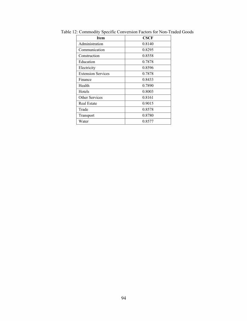
94
Table 12: Commodity Specific Conversion Factors for Non-Traded Goods Item CSCF
Administration 0.8140 Communication 0.8295 Construction 0.8558 Education 0.7878 Electricity 0.8596 Extension Services 0.7878 Finance 0.8433 Health 0.7890 Hotels 0.8003 Other Services 0.8161 Real Estate 0.9015 Trade 0.8578 Transport 0.8780 Water 0.8577

[This page is intentionally left blank]

96
Annexure C: Economic Opportunity Cost of Labor

97
Estimation of The Economic Opportunity Cost of Labor: An Operational Guide for Kenya
1. Introduction
The need to measure the social or economic opportunity cost of resources arises whenever such
resources are diverted from current uses (or non-use) to a government project. The economic
acceptability of any proposed project depends upon the cost and benefit streams expected over the
lifespan of the project, and a vital aspect of any cost-benefit analysis is how to determine the proper
values to the resources required as inputs.
For the specific case of the labor input, when workers are hired by a project, they are giving up
one set of market and non-markets activities for an alternative set. The economic opportunity cost
of labor is the value to the economy of the set of activities given up by the workers, including the
non-market costs (or benefits) associated with the change in employment. Jenkins (1995)
Employment is often a hot topic when it comes to any government in the world, as it is a primary
macroeconomic objective. For years, governments in many countries have actively promoted
creating employment for people to mitigate their relatively high unemployment rates. For any
project to be economically justified, the net present value of the net economic benefits of the
project must be positive. One of the most important benefits is the labor externality (LE) from the
jobs created by a project, which can be estimated by the difference between the wage paid on the
project and the economic opportunity cost of labor.
LE = Wp− EOCL (1)
When this value is positive, it implies that the financial cost of labor will be greater than its
economic cost. The LE can split between the worker and the government. The magnitude of LE is
related to several factors, including the supply conditions of the type of labor being employed.
This analysis, however, will illustrate that additional elements such as social security programs,
income taxes, and union monopoly power also need to be considered.

98
The purpose of this study is to show how economic theory can be empirically applied to estimate
the economic opportunity cost of labor for public projects in the Kenyan economy. Given that
labor is a highly heterogeneous production factor, estimating the EOCL would not be an easy task.
Typically, the labor market experiences different dynamics across occupations, skills, working
environments, labor market conditions, and regions. Thus, the EOCL will also vary across these
situations.
The variability of the EOCL necessitates the need to develop an operational estimation
methodology that quantifies this opportunity cost across occupational groups and different labor
markets with an acceptable degree of accuracy. In this vein, the current work provides an
operational guide to estimating the EOCL for various skills and labor market types applicable to
Kenya.
The study is organized as follows; after this introduction, the second section gives an overview of
the Kenya labor market and some of its essential aspects. Section 3 describes the methodologies
applied in this guide and discusses its associated advantages. Section 4 considers eight cases
involving seven cases dealing with domestically sourced labor relevant to Kenya, while the last
case considers foreign labor employment. Finally, concluding remarks are presented in the fifth
section. An Excel model is accompanied to this study to allow the project analyst to estimate the
value of EOCL for the specific type of labor employed.
2. Labor Markets in Kenya
Kenya is ranked as a lower-middle-income country and has become the third-largest
economy in sub-Saharan Africa with well-organized industrial relations. The economic growth has
been robust, along with increasing wages; however, structural challenges affect the labor market.
Kenya's economy is characterized by a formal sector experiencing an environment of shrinking
employment opportunities and an informal sector that is increasingly expanding and absorbing
entrants from schools and training institutions to the labor market. The failure of the formal sector
to generate sufficient wage employment to accommodate all entrants to the labor force has led to

99
many youths starting their businesses or seeking employment in the informal sector. (Kenya
National Bureau of Statistics, 2020b)58.
The employment structure has changed over time with the informal sector expanding into
manufacturing, transport and information, communication, and technology and taking a leading
role in job creation. In 2019 the informal sector was estimated to have created 767.9 thousand new
jobs, constituting 90.7 percent of the total new jobs created outside of small-scale agriculture. The
informal sector's contribution to total employment has increased from 10.4 percent in 1972 to 46.9
percent and 83 percent in 1992 and 2019, respectively,59 which is shaded by non-compliance with
labor regulations (including wages).
Bigsten and Wambugu (2010) argue that the increase in informal sector firms leading to the
employment expansion in the sector is mainly made possible by the limited capital requirements
for new jobs in the sector. The formal sector employment expansion, on the other hand, has been
constrained by the inability of the country to achieve rapid capital accumulation to improve on the
capital-labor ratio and the labor market regulations that have tended to increase labor costs relative
to productivity in the sector.
Kenya's employment composition by sector has been relatively stable during the last decade and a
half. The agricultural sector contribution of total employment is estimated to decrease six
percentage points from 61% in 2005 to 55% in 2019. It remains by far the most significant sector
measured by numbers of employed.60 However, fluctuations in employment demand reflect on the
weather effects with significant dips experienced during severe droughts. In the period from 2005
to 2019, the service sector has increased seven percentage points to 39%. The industry sector has
remained its size at 6% share.
Like in most countries, especially Sub-Saharan Africa, the labor market in Kenya experiences an
internal rural-urban migration. Rural areas accounted for two-thirds of the total jobs in the
informal sector, which means that labor supply is high in rural areas.61 The country has
58 See Informal Sectors Skills and Occupations Survey (ISSOS), 2020.
59 See Economic Survey 2020.
60 Source: International Labour Organization, ILOSTAT database. Data retrieved on January 29, 2021.
61 See Economic Survey 2020. Table 3.11, Persons engaged in the informal sector by activity.

100
recorded a steady rise in urbanization. In 1950, the share of the urban (rural) population was 7.36
percent (92.64 percent). In 2019, the urban population increased to 27.99 percent, while the rural
population has declined to 72.01 percent of the total population due to rural-urban migration
resulting from the pull factors in urban areas (quality of life and economic opportunities in urban
areas, among others).
The higher minimum wages in urban areas have been identified as one of the contributing factors
to rural-urban migration in developing countries. Migration of labor can also partly be attributed
to insufficient support extended to agricultural production and low prices for farm produce. The
labor movement is explained by the availability of greater opportunities in urban areas with the
most educated workers migrating in search of jobs. (M Wangi et al., 2017).
According to Agesa (2001), in Kenya, the gap between expected urban and rural wages and higher
levels of education encourages rural-to-urban migration as the returns for higher productivity are
greater in cities. Agesa and Agesa (2005) investigate the factors that influence Kenyan rural-urban
migration. They found that the wage gap between migrants in urban areas and non-migrants in
rural areas greatly increased the likelihood of males migrating from rural to urban locations.
It has also been common over past years in Kenya for certain groups of workers to relocate abroad
with the hope of improving their fortunes. Kenyan emigrants to the United Kingdom, United States
of America, Canada, and South Africa being skilled and educated and leave for employment or
education abroad through traditional means (UNDESA, 2019). Increasingly, low-skilled Kenyan
migrant workers migrate to the Middle East and the Gulf countries for work, as job opportunities
are generally more than in other regions.
Despite a large and growing supply of labor in general, foreign workers are brought in by
corporations or the government for projects requiring their skills. In Kenya, this often takes the
form of high skilled labor or technical staff. According to Song (2016), the estimated number of
Chinese migrants living and working in Kenya is between 80,000 and 100,000; they are also well-
educated and are typically employed by construction companies.

101
In light of the foregoing, this study focuses on a number of scenarios that demonstrate how the
EOCL should be calculated in each of these situations. Now we turn to a discussion of the
methodology.
3. Methodology
The challenge of measuring the economic opportunity cost of labor is a subject of considerable
discussion in the economic literature, which can be summarized into two alternative methods:
foregone product and supply price. The fundamental consideration in the foregone product
approach is to take the current technology and market structure as given and try to determine the
value of the marginal product foregone when a worker is added to the public payroll.62 The second
approach is via the supply price of labor which is defined by Harberger (1972) as the amount for
which a worker is willing to present himself for work at a specific project site.
The supply price is an ideal measure in the sense that it is location-specific and implicitly includes
the value of a foregone product as well as the value of all other monetary and non-monetary
sacrifices that the worker makes when he presents himself at the project site. The easiest way to
think of the economic opportunity cost of labor in a given area, occupation, industry, or other
category is to start with the market wage and make a series of adjustments. All the labor of each
type earns its relevant market wage. (Harberger, 1985). This analysis employs the latter approach
as it is generally more straightforward and applicable across varying labor market conditions and
has less stringent data requirements.
When employing the supply price approach, we first consider the gross tax wage that employers
need to pay in order to obtain sufficient workers of a particular skill. This variable is also generally
well-known amongst employers operating in the region of the project. It is the net of tax wage;
however, that potential employees are responding to when choosing to work on the project or not.
An advantage of this approach is that the net of tax supply price already captures the worker's
preferences for location, working conditions, and other idiosyncratic factors which may affect their
decision to work on the project. From the individual's perspective, this price reflects the economic
cost of supplying labor to the project.
62 This approach has been initially proposed by Little and Mirrlees (1968).

102
The marginal product foregone approach would require the project analyst to estimate the
monetary values of each of the components individually and accordingly adjust the foregone wages
for the equalizing differences in well-being and costs as valued by the worker between the
employment and living conditions of the alternative employment situations facing the potential
project employee. This generally cannot be done with an acceptable degree of accuracy, given the
time constraints associated with the appraisal of the project.
If a project hires labor, we should expect some people already employed in other places to move
to the project. These workers will migrate to the project if their project wage is at least as large as
their required supply price. This labor market adjustment will decrease the quantity supply of labor
supplied in the alternative labor markets. It is important to note that if a labor market is
characterized by a high level of unemployment, this fact will tend to lower the supply price (gross
of tax wage) that the workers would require before offering their labor services to the project. The
opposite is also the case when a particular labor type is in short supply. Here we would expect to
find that the supply price of this type of labor will rise.
Once the gross of tax supply price (wage) for the project is determined, it is adjusted to account
for the various distortions present in the labor market. It is critical to incorporate all the relevant
distortions to estimate the EOCL accurately.
These distortions arise from the presence of income taxes, social security contributions,
employment insurance, labor union monopoly power, enforced minimum wage laws, or any other
type of tax or subsidy present in the project's labor markets. Furthermore, when workers move
from an alternative job to work on the project, they will consider the net of tax wage they are
giving up and the minimum net of tax wage they must receive to be willing to work for the project.
If they pay taxes on the wages they earn in their alternative employment, they will not consider
these taxes lost as a loss in economic welfare.
While the reduction in tax revenues from the reduction in employment is not in itself an economic
welfare loss, however, the worker must have been generating a value of a product in the alternative
employment large enough, so the employer is willing to pay a gross of tax wage sufficient for the
employee to earn his/her supply price for that job and at the same time be able to pay the tax on
these wages. This component of the value of the marginal product of labor that serves to cover

103
the cost of these taxes is an economic loss that the worker does not consider when moving to the
project from alternative employment. Hence, two adjustments need to be made to the gross of tax
supply price associated with the project. First, a subtraction must be made of the tax component
of this supply price for the project site and an addition to an amount that is measured by the taxes
no longer paid where a worker moves from the alternative place of employment.
When a project hires additional employees, it is natural that some new workers may represent new
entrants to the formal labor force in response to the improved labor conditions created by the
project. These new entrants will be responding to the opportunity to earn a net of tax wage that
will be paid by the project. If there are no taxes or subsidies associated with their prior non-formal
market activities, then the gross of tax wage rate reflecting the supply price to the new project only
needs to be adjusted by the taxes that will be paid by the new labor force entrant earning this supply
price-wage. In the absence of taxation, worker migration for employment on a new project from
employment in an alternative market requires no adjustment to drive the EOCL. The supply price
captures exactly the lost benefits of the worker in the alternative market.
In summary, when labor markets are competitive, the estimation of the EOCL begins with the
gross of income tax supply price of labor; Wgs for a particular type of labor skill that will be
supplied to a specific project at a given location. This wage, Wgs, reflects the minimum wage that
the project would need to offer in order to meet its labor needs. This simple measure captures a
number of important factors. For instance, this wage already accounts for the worker's skill level,
its preferences regarding location, working conditions, the disutility of moving to the project, time
spent away from family or household production, and the alternative employment opportunities
available to the person. In a market with no distortions, this supply price wage for a type of labor
captures the EOCL as it captures all of these foregone opportunities for the worker. This is, in
essence, the advantage of the supply price approach to estimating the EOCL of labor.
3.1 Methodology for Estimation of the EOCL in the presence of taxes and other
distortions.
When distortions are present in the labor market, we must adjust the supply price to account for
these. The two most common distortions in the labor market are income and social security taxes.
Income tax is levied on the growth of income wage received by the employee. Typically, the

104
responsibility for the payment of income tax is on the individual employee. However, the employer
might be required to withhold the estimated income tax at the time wages are paid. The tax base
for social security tax is also the wage gross of income tax paid by the employer to the employee.
However, the amount of this tax is calculated by the employer and paid to the government. From
the perspective of the employer, the total employee compensation or payment is the project wage
()!) plus the social security paid by the employer (*"). These two added together to become the
total employee compensation 1GH = 1G(1 + +:).
When the wages are subject to income taxes, the EOCL becomes the gross-of-tax supply price to
the project less the income taxes paid by this worker on the project plus any tax lost as a
consequence of the movement of labor to the project. We can denote the share of the project's labor
sourced from currently employed workers as Hd. These workers earn the alternative wage Wga.
The remainder of the project's labor would be sourced from the informal sector or non-market
activities, which does not require adjusting for income taxes 63. In what follows, the degree of
distortions in the market is the most relevant factor.64 In the case of the presence of distortions, the
EOCL is:
EOCL = Wgs - (Wg
s T – Hd Wga T’) (2)
where:
• Wgs denotes the gross of income tax supply price of labor.
• Wga denotes the gross of income tax wage of labor from alternative sources.
• T denotes the income tax rate plus social security paid by employees corresponding to the
supply price of labor.
• T' denotes the total effective tax rate, including both the income tax rate and the social
security taxes (*" + *"#) corresponding to the alternative wage rate.
• T" denotes the income tax rate plus social security paid by employees corresponding to the
project wage, levying on wages in the formal sector.
63 The tax structure applicable to labor income in Kenya is detailed in the Appendix.
64 Jenkins, Glenn P., and Arnold C. Harberger. Cost-Benefit Analysis of Investment Decisions,2019.
105
• Hd denotes the proportion of the project's demand for labor obtained from taxed
employment in the alternative market.
In equation (2), the supply price of labor is adjusted (reduced) by the income tax rate levied on the
wage paid to the project's labor force (Wgs T) and is increased by the income and social security
taxes lost from reduced employment in the alternative formal labor market (Hd Wga
T'). In the case
of Kenya, Hd is a particularly important parameter. Because the informal sector makes up such a
large portion of economic activity, it may be reasonable to assume that a great deal of labor comes
from informal market activities as opposed to alternative formal markets. As such, we would
expect a reasonable parameterization of Hd for Kenya to be lower than for a county where the
informal sector is less substantial.
From equation (2), we can calculate the labor externality associated with a project when distortions
are present. We present the general case here and illustrate the calculation of this externality
alongside the estimation of the EOCL below. Again, from equation (1), the labor externality is:
LE = )!$ – EOCL = )!$ – [Wgs + (Wgs T – Hd Wga T')] = Wp (1+*") – [Wgs + (Wgs T – Hd Wga T’)] = Wp + Wp**"- Wgs - Wgs T + Hd Wga T' = Wp T’’+ Wp (1-T)’’+ Wp**"– [Wgs (1-T) + Hd Wga T’] (3) We can interpret each of the terms above as being benefits accruing to labor or taxes gained (+) or
lost (-) by the government:
Labor benefits = Wp (1-T’’) - Wgs (1-T) (4)
Government benefits = Wp T’’ + Wp**"– Hd Wga T (5)
4. Economic Opportunity Cost of Labor
This study will now apply the supply price of labor approach to estimate the EOCL used by
projects for different situations relevant to Kenya. Firstly, we will evaluate the EOCL on rural and
urban projects, hiring skilled and unskilled labor from domestic markets. We will also illustrate
the EOCL for the case of a project in Kenya hiring domestic labor who can alternatively work
abroad. We will then turn to the issue of hiring foreign labor employed in Kenya. We will illustrate
each case analytically, followed by an empirical illustration.

106
4.1 A Rural Project Employing Domestically Sourced Unskilled Labor
In the first case, the EOCL is estimated for an unskilled labor market with no significant distortions
exist. i.e., the employer (demand side) does not pay taxes, and the worker (supply side) does not
pay income taxes. It is further assumed that wages or labor demand have no fluctuations over time.
Suppose a project in a rural region employs unskilled labor at the prevailing market monthly wage
rate. In this case, the EOCL is the simple calculation described above. Beginning with the gross of
tax supply price of labor, Wgs, the EOCL is:
EOCL = Wg s (6)
Because no distortions are present, the market wage is the supply price that captures all the factors
mentioned above and thus reflects the true EOCL for this type of labor. Suppose the approximate
monthly market price of unskilled labor in a rural area in Kenya is KES 4,42265, and the project
will pay an amount equal to the supply price of labor (Wg s= Wp). The EOCL is then:
EOCL = Wgs = KES 4,422
Using equation (1) for the estimation of labor externality, the LE associated with this project is:
LE = 1GH – EOCL
However, given that no social security payments would be applied, the )!$ is equal to Wp which
results in no labor externality (LE=0).
As can be seen from the above, there is no LE in this first case. Because no distortions occur in
this market, there is no externality generated from the reallocation of labor to employment by the
project from other activities. If unemployment is high in the region, then the supply price of labor
65 The gazetted monthly basic minimum wages for unskilled workers in the agricultural industry is KES 6,736. There is evidence that formal sector earnings are consistent with the
regulation of wages guidelines; however, the informal sector still lags behind in complying with regulations. According to the Informal Sectors Skills and Occupations Survey
(ISSOS) 2020, the mean monthly earnings of a skilled farm fishery wildlife and related worker in the informal sector of rural areas is KES 5,476. As the unskilled worker receives
wages almost 1.5 times lower than those of skilled workers, the monthly market price of unskilled labor in a rural area is approximately KES 3,650. The Economic Survey Report
of 2019 identifies informality as a prominent feature in the Kenyan economy, representing about 83% of the total employment in the country. Based on these facts, we assume that
half of the workers are coming from the average wage rate of the informal sector, and the other half are coming from the average wage rate of the formal and informal sector's wage
rates. Therefore, we estimated the monthly supply price of unskilled labor in rural area to be KES 4,422: 0.5*3650 + 0.5 * ((6736 + 3650)/2).
107
to the project as reflected by the market wage will be lower than it would be if the incidence of
unemployment were less.
An important consideration when determining the EOCL, particularly in rural regions, is that labor
allocation in the agricultural sector is greatly affected by the seasonality of agricultural activities.
Seasonal changes in agricultural activities (land preparation, planting, weeding, tending crops,
harvesting) result in both slack periods and peak periods of work, which in turn generate troughs
and peaks in demand for rural labor. Consequently, the prevailing market wage will vary from one
season to another.
This seasonal variation in the wage rate for a particular type of labor can affect the EOCL
considerably. It must be accounted for in the estimation of the EOCL for labor employed for an
extended period of time, such as one year. The pattern of the seasonal project demand for a
particular type of labor also determines the overall EOCL for the project.
Seasonal variation in both the market wage and the labor needs of the project must be accounted
for to estimate the EOCL accurately for the entire amount of unskilled labor employed by a project
over the year. Equation (7) deals with this matter by expressing the EOCL for a project as the
product of the monthly market wage rates (Wt) and the labor demand (Lt) for each season (month),
in a location or region over the course of a year. This can be expressed as:
EOCL = ∑ ?2ICJK 12 (7)
Where t denotes a specific period of time and n represents the total number of time periods.
In a country that is as geographically and culturally diverse as Kenya, there will not be complete
uniformity of agricultural seasons between the different parts of the country. There is variability
in the level and pattern of rainfall in the different regions of Kenya, just as there are variations in
the quality of the soil, the altitude, and the desires (tastes) of the different ethnic groups for various
agricultural products.66
66 In most parts of Kenya, the rainy season runs from March to May. Many crops are planted during this time, with harvesting after the rains, with the length of time varying
depending on the crop's growth season. There is a secondary rainy season in several parts of the nation that can occur at any time between July and December, depending on the
region.

108
To illustrate, consider Table 1, which depicts a monthly market wage schedule and labor demand
(in person-months) over the course of a year for a particular project designed to coincide with the
agricultural cycle in a specific region in Kenya, which starts with land preparation from December
to February, followed by planting activities in March. Planting is followed by weeding between
April and May. In June, early crops start to become available, and harvest begins in earnest in July.
In August, few agricultural activities take place.
Applying equation (7) to the data in Table 1, the annual EOCL for the project as a whole is:
EOCL = ∑ ?2ICJK 12
= (4250*10 + 4250*10 +6000*15 + ...… + 4250*5) = KES 419,170 Suppose the wage paid by the project is KES 6736. The financial cost to the project of hiring
unskilled labor for the year is the project's wage times the 75 person-months of labor or KES
505,200. The difference between this amount and the economic opportunity cost is the value of
labor externality. In this case, a project wage is not great enough to be subject to income taxes.
With no social security tax, the entire amount of externality accrues to labor hired by the project
as a net distributional benefit.
LE= (Wp *n) – EOCL
LE = ((6736 * 75) – 419,170) = KES 86,030 for the project.
Labor Benefits (LB)= (Wp*n) - ∑ ?2ICJK 12 = 505,200 – 419,170 = 86,030 KES per Month
Fiscal Benefits (FB) =0
Table 13 Market Wages and Labor Demand for a Project with Seasonal Agriculture
Month Regional Market Wage (KES /month)
Labor Demand/person, Month by Project
EOCL of Total Project Labor by Month (KES)
January 4250 10 42,500 February 4250 10 42,500 March 6000 15 90,000 April 6000 5 30,000 May 5820 5 29,100 June 6736* 5 33,680 July 6736 15 101,040
August 5820 5 29,100 September 5000 0 -
October 4250 0 - November 4250 0 - December 4250 5 21,250
Total ----- 75 419,170 * The higher wage rates in June and July reflect the fact that the harvesting season of many crops may coincide with the planting season of the secondary rainy season in some
regions in Kenya.

109
4.2. A Monthly Rural Project Employing Domestically Sourced Unskilled Labor from
the Informal Sector to the Rural Formal Sector Jobs.
When a worker becomes employed in the formal sector of the economy, social security taxes must
be paid on the wages they receive.67 The only social security tax levied in Kenya is the National
Social Security Fund (NSSF). The NSSF is a statutory savings scheme to provide for retirement.
These social security taxes are 12% of the pensionable wages made up of two equal portions of
6% from the employee(*"#) and 6% from the employer (*") subject to an upper limit of KES
2,160 for employees earning above KES 18,000. The employee contribution shall be drawn
directly from his salary and wages, while the employer's contribution shall come directly from the
employer.68
The analysis will begin with the assumption that the formal sector project pays a competitive wage
so that the equation of ()!(1 − *"#) = )%"(1 − *"#)) must be valid. As the worker is moving
from the informal sector to the formal sector, then the social security tax rate *"# was levied on
the supply price of labor in the informal sector is equal to zero. Hence, we have
()!(1 − *"#) = )%"). This equation states that the employee's net of social security wage they
receive is equal to the supply price of labor which in turn is the prevailing market wage in the
informal sector. Alternatively, the project wage)! must be at least equal to &./
#'(/0. Iftheprojectwereto paid less, then the workers would be worse off working for the
project than working in the informal sector.
The cost of this labor to the project will have to include the wage rate paid to the employee plus
the 6% social contribution that, by law, the employer must pay. For unskilled labor jobs, it is
assumed that the wage rate is not high enough for the individual to be subject to income tax. Hence,
the project wage (employer's cost )!$) is higher than the supply price (Wgs ) of unskilled labor for
67 The NSSF pension fund is supposed to provides basic financial security benefits to Kenyans who work in the formal and informal sectors of the economy. According to Kenya
Social Protection Sector Annual Report 2018/19 (2020) only 15% of all workers aged 18-65 years in the country have an employer contributing to NSSF pensions, and it is expected
that only a small extent of this percentage is an informal sector worker.
68 These rates are based on the New NSSF legislation (the NSSF Act 2013) was enacted on 24 December 2013 to replace the NSSF Act Cap 258. The new legislation was scheduled
to take effect on 31 May 2014, but the effective date for the legislation was delayed.

110
this formal rural project by a total of 12%. In this case, the EOCL= )%", but the LE is equal to )!$ –EOCL. Here the )!$ equals to 1.06* Wp.69
If the monthly market wage of unskilled labor in the informal sector (supply price )%") is 7,137
KES70, then at least the project wage (Wp) of this unskilled labor in the formal sector is
Wp = )12#'*20
= 7,137/1-0.06 = KES 7,593.
Then the labor cost to the project is therefore equal to
)!$ =1.06* Wp
)!$ = 1.06*7593= KES 8,049
Given that EOCL= )%" = 7137, then the LE is:
LE= )!$ -EOCL=8049 - 7137 = 912 KES per month.
As can be seen from the preceding, the monthly labor externality created in this case accrues to
the government in the form of social security tax revenues.
The rate of government benefits which represents the benefits accrues to the government (fiscal benefits)
to the total compensation for the employee, equals to: L%(M:NM'()L%(ONM:)
= PQRS∗K.OU
PQRS∗O.KV= 0.11.
The ratio of the EOCL relative to the total compensation for the employee ()!$) is called the
conversion factor (CF) for this specific type of labor. This quantity can be used to convert a project
wage to its EOCL. In the above case, the conversion factor is CF= EOCL/W′p = 7137/8049 =
0.89.
69 It is worth to note that if the employees wage rate to be paid is KSh 18,000 and above, the maximum amount to be paid by the employer is KSh 1,080. In other words, if the wage
rate is greater than KSh 18,000, then the effective social security tax rate would be less than 6 percent.
70 According to the Informal Sectors Skills and Occupations Survey (ISSOS) 2020, the mean monthly earnings elementary occupations in the informal sector of rural areas is KES
6,727. Taking into account that the monthly minimum wage rate for miner, stone cutter, turn boy, waiter, cook, logger, line cutter in in (all other towns rather than Nairobi, Mombasa,
Kisumu Cities Mavoko, Ruiru and Limuru cities) is KES 8,366 which approximately reflects the wage rate in the formal sector, we estimated that the monthly supply price of this
category of unskilled labor in rural area to be KES 7,137: 0.5*6727 + 0.5 * ((6727 + 8366)/2).
111
4.2.1. Monthly Wage in Formal Sector Is Higher Than the Prevailing Market Wage Rate
Suppose this formal sector employer pays a monthly wage that is 20% higher than the prevailing
market wage rate (supply price), then the Wp is now equal to 7137 *1.2 = 8,564 KES per month.
As a result, the project wage (employer's cost) ()!$) is equal to 1.06 * 8564=9,078 KES.
In this case, the level of income is not great enough to be subject to income taxes; however, we
have the social security tax of*"# = 6% paid by the employee.
In this case, similar to the case above, the EOCL is taken as the private supply price irrespective
of what financial wage the project pays.
Given that EOCL= Wgs = 7137, then the LE is:
LE= 1GH -EOCL=9078-7137=1,941 KES per month.
LB= *3(1 − *"#) −Wgs = 8564*(1-0.06)-7137= 913 KES per month
FB= Wp *"# + Wp**"=8564*0.06 + 8564*0.06=1028 KES per Month
In this case, the conversion factor is CF = EOCL/W′p =7137/9078 =0.79. The conversion factor
has been reduced as the project wage has surpassed the labor supply price.
Table 14 Summary Statistics for Rural Unskilled Labor in the Formal Sector
4.3. A Rural Project Employing Domestic Skilled Labor with Migration from Other
Labor Markets
This case considers a project that demands skilled labor in a remote region where such labor may
not be available. The supply price of this labor in this region is likely to be higher than what this
Case
Monthly project wage ( Wp )
Monthly supply price
of labor ( Wg
s )
Total labor compensation
())*)
Alternative wage rate ( Wg
a ) EOCL +. %
'-))*
'.))*
%.))*
Rural, Unskilled,
Formal Sector 7593 7137 8049 ---- 7137 0.89 0.11 0 0.11
Rural, Unskilled,
Formal Sector 8564 7137 9078 ----- 7137 0.79 0.21 0.10 0.11

112
labor would have been earning in the alternative urban labor markets for such skilled labor in order
to derive equal utility. This is due to the fact that working conditions, costs of living, and locational
preferences differ between regions.
The rural project's net of tax wage rate must be at least as high as the net of tax supply price of this
labor. To retain enough skilled workers, the project wage may be higher than the prevailing market
wage for a given skill in the project's area in some cases. Because the new work is in the formal
sector, social security contributions must be taken into account.
When a person is employed in a market where a personal income tax exists, the EOCL is
determined by the value this individual receives by supplying his labor services, which would be
measured by the wage net of personal income taxes. In this case, the EOCL becomes the supply
price less the amount of income taxes paid by this individual working at the supply price, plus the
foregone income taxes that would have been generated elsewhere in the economy if the worker
had not moved to the project region.
As a share of the project's labor, Hd will be sourced from taxed employed workers earning the
alternative wage Wga, perhaps even in other parts of the country. The remainder of the project's
labor would be sourced from the informal sector or non-market activities, which does not require
adjusting for income taxes. As discussed before, in the case of the presence of distortions, the
EOCL is:
EOCL = Wgs - (Wg
s T – Hd WgaT’)
From equation (3), we can calculate the labor externality associated with a project when distortions
are present.
LE = Wp T’’+ Wp (1-T’’) + Wp**" – [Wgs (1-T) + Hd Wg
a T']
Using the equations (4) and (5) as presented in the methodology section, provide the benefits to
labor and to the government as following:
Labor benefits = Wp (1-T’’) - Wgs (1-T)
Government benefits= Wp T’’+ Wp**" – Hd Wga T'

113
For this illustrative example, we focus on a specific subset of skilled labor with a skill at the third
to fourth ISCO skill level, such as professional services. Assume the skilled professional labor
require a monthly wage of KES 31,413 gross of tax and social security contributions (the supply
price (Wgs)).71 Suppose the alternative wage rate (Wa) is 80% of the supply price (KES 25,130).
In addition to this, the supply price of labor (Wgs) net of all taxes must be equal to the project wage
(Wp) net of income and the social security taxes paid by the employee. This will be the lowest
wage the project can pay and expect to get skilled labor to work for them. Incorporating the
effective income tax rate and social security contribution rates described in the appendix, the
individual would pay an income plus social security tax rate (T") of 9.34% on the project wage
(Wp) while the tax rate corresponding to the alternative wage rate (T') is 9.72% and the income
tax rate of the supply price of labor (T) is 9.34%. Hence, the relationship will hold that in this case,
Wp (1-T") = Wgs (1-T). Therefore, the total employee compensation (1GH) is equal to [Wp (1++:)] =
31,413 ∗ 1.0344 = 32,493)'"QRSTUV2ℎ]72. We again assume that Hd = 0.9, given the relative
tightness of the skilled labor market. The EOCL can then be estimated for this skilled labor by
combining the supply price for the worker with the tax gains and losses associated with this
employment. Following equation (2):
EOCL = Wsg - (Ws
g T – Hd Wga T’)
= 31413 – (31413*0.0934 – 0.9*25130*0.0972) = 30,678 KES per month The labor externality (LE) is estimated as the difference between the employer's financial cost and
the EOCL for this type of skilled worker. The excess of financial wage over the economic cost
reflects a net benefit to labor and government.
The total labor externality LE = )!$ - EOCL = 32,493 – 30,678= 1,815 KES per month
From equations (4) and (5), we can calculate the benefits of the labor to the project and to the
government, and thus the magnitude of the labor externality:
Labor benefits = Wp (1-T’’) - Wgs (1-T)
= 31,413 (1 – 0.0934) – 61,413 (1 – 0.0934)
71 International Labour Organization (ILO) Mean nominal monthly earnings of employees by sex and occupation (2019).
72 The employees wage rate exceeds KSh 18,000, however, the maximum contribution to be paid by the employer is KSh 1,080. Therefore, the effective social security tax rate
would be 1,080/31,413=3.44%.

114
= 0 KES Government benefits = Wp T"– Hd Wg
a T’+ Wp**" = 31,413*0.0934 – 0.9*25,130*0.0972+31,413*0.0344 = 1815 KES
The sum of these two quantities is, by definition, the total labor externality:
LE = 1,815 KES per month.
The entire externality is a net gain in government revenues; however, the labor benefits are equal
to zero as the supply price of labor (Wgs) equals the project wage (Wp).
In terms of the conversion factor, it is calculated by the ratio of the EOCL to total employee
compensation (1GH). In the above case, the conversion factor for labor when the project pays a wage
equal to the gross of tax supply price adjusted for the social security tax is 30,678 /32,493= 0.94.
4.3.1. The project wage (Wp) is above the supply price of labor (Wgs)
Now suppose that the project wage (Wp) is substantially above the supply price of labor (Wgs). Let
us assume that the project wage is 20% more than the supply price of labor for workers being
employed by the project. Hence, we have 1G =1W:(1 + 0.2) = 31,413*1.20= 37,696 KES.
Accordingly, the total employee compensation must include the social security tax and is equal to (1GH = 83,366 ∗ 1.0287 = 38,776)'").73
The income tax plus the social security rate (T") corresponding to the project wage is estimated to
be 12.66%. In comparison, these combined income tax rates plus the social security for the supply
price of labor (T) is 9.34%. The T' which is tax rate (income tax plus social security) corresponding
to the alternative wage as before, is 9.72%. Using these statistics in the example above, the EOCL
can then be estimated as,
EOCL = Wsg - (Ws
g T – Hd Wga T’)
= 31,413– (31,413*0.0934 – 0.9*25,130*0.0972) = 30,678 KES per month.
73 The effective social security rate in this case is 2.87%: 1080/37,696.

115
Accordingly, the conversion factor is 30,678/ 38,776= 0.79.
There is a net gain of KES 8,098 per month of employment of a skilled worker hired by the project
because the EOCL for this type of labor is only KES 30,678 while the financial wage paid by the
project is KES 38,776. The gains accrue in part to workers due to the higher wage paid by the
project and in part to the government because of the gain in tax revenues.
Considering both components and applying equations (4) and (5):
Labor benefits = Wp (1-T”) - Wgs (1-T)
=37,696 (1 – 0.1266) – 31,413 (1 – 0.0934) = 4,445 KES Government benefits = Wp T"– Hd Wg
a T’+ Wp**" = 37,696 *0.1266– 0.9*25,130*0.0972 + 37,696 *0.0287 = 3,653 KES Both labor and government benefits add up to the total labor externality: 4,445+3,653=8,098.
Table 15 Summary Statistics for the Rural Skilled labor in a Formal Sector
4.4 An Informal Urban Project Employing Locally Sourced Unskilled Labor at the
Supply Price
An urban project is drawing upon unskilled labor from the informal sector. In this case, we assume
that the project pays a wage equal to the prevailing market wage, which is equal to the labor supply
price ()! = )%").
Unskilled workers in the informal sector typically do not pay social security contribution on the
gross of income tax wage )!, moreover, the typical project wage is not enough to meet the income
tax threshold level. Hence, the project wage (employer's cost )!$) is also equal to the project wage
(Wp).
Case Monthly
Project wage ( Wp )
Monthly Supply price of labor
( Wgs )
Total Labor Compensation
())*)
Alternative Wage Rate
( Wga )
EOCL C.F '-))*
'.))*
/.))*
Rural, Skilled, Formal Sector 31,413 KES 31,413 KES 32,493 KES 25,130 KES 30,678 KES 0.94 0.06 0 0.06
Rural, Skilled, Formal Sector 37,696 KES 31,413 KES 38,776 KES 25,130 KES 30,678 KES 0.79 0.21 0.115 0.095

116
In our analysis of the EOCL for workers employed in the informal sector of an urban economy,
we recognize a close relationship between the labor market conditions of the urban areas and those
of the rural economy. Migrants move into the urban sector from the rural (Countryside) as urban
areas have more concentration of businesses than the rural areas. Furthermore, Agesa and Agesa
(2005) mentioned that the difference between the expected wages for migrants in urban areas and
non-migrants in rural areas in Kenya significantly increases the likelihood of rural-to-urban
migration, mainly for males. Brauw et al. (2014) found that in six sub-Saharan African countries,
including Kenya, the urban informal wages are more than double of the rural informal wages.
Clearly, there appears to be a high return to moving from the rural to the urban informal sector in
such countries.74
However, there is a growth of negative externalities or fiscal costs associated with the rural-urban
migration process that the unskilled informal sector workers do not pay for. These negative
externalities may include increased congestion of public services and transportation, additional
crime and resulting additional security costs, pollution and government subsidies associated with
increased access to health services. These pose additional economic costs on society or the
government that should be reflected in the EOCL. In our example, we account for these external
costs simply as a percentage K of the gross of tax supply price of labor. In the example below, we
assume that this negative externality equals 6 percent of the prevailing urban market wage for
unskilled labor.75 In this case, the EOCL= Wgs+K* Wgs, and the LE is equal to )! –EOCL.
Suppose a project in the urban area hires an unskilled worker in the informal sector. The assumed
monthly wage (supply price) of an individual is KES 8,417,76 the labor cost to the project is,
therefore, equal to:
)!$ =Wp = 8,417KES
EOCL= 8417+0.06*(8417) = 8,922, then the C.E is:8922/8417= 1.06
74 This finding is consistent with the Informal Sectors Skills and Occupations Survey (ISSOS) results for Kenya which show that informal sector employees located in the urban
areas have two times higher average monthly earns compared to their counterparts in rural areas. 75 Michaud, P. C., & Vencatachellum, D. (2003). Human capital externalities in South Africa. Economic Development and Cultural Change, 51(3), 603-628.
76 This wage represents the informal sector’s mean monthly earnings of employees in elementary occupations in urban areas in Kenya. See, Informal Sectors Skills and Occupations Survey (ISSOS) 2020.

117
LE= )! –EOCL= 8417-8922= - 505 KES.
This amount of externality is incurred as a fiscal cost by the government.
Table 16 Summary Statistics for the Urban Unskilled labor in Informal sector.
4.5. A Formal Urban Project Employing Locally Sourced Unskilled Labor at the
Supply Price
Suppose now we have a project in the formal sector in an urban area. This project requires unskilled
labor, pays the required social security tax to the government, and deducts the portion of the social
security tax levied on the worker's wages paid to the government. We assume that the project wage
is not enough to meet the income tax threshold level. The negative fiscal externality exists
associated with the resulting rural-urban migration that they do not pay for.77 Similar to the above
case, we assume that this negative externality equals 6 percent of the prevailing market wage
(supply price) for unskilled labor in the urban sector.
For this type of labor, the minimum wage that can be paid to attract workers to this project must
be such that the amount net of social security tax at least equals to the supply price demanded by
this type of worker. If the monthly supply price of labor in the urban area )%" =11,112 KES,78
then the competitive monthly project wage must beW+= 1/(1-Ts1) = 11,112/(1-0.06) = 11,821.
The EOCL is expressed as: EOCL = Wg
s + Wgs K
77 Rural unskilled workers with little or no human capital skills may migrate to urban areas. In the case of Kenya, Oyvat & Gĩthĩnji, (2020) found that individuals who have low
skills and are pushed out of their home rural district by the lack of land migrate to smaller urban centers or other rural areas. Migration to Nairobi, which is more expensive, seems
to require higher skills and wealth.
78 The monthly supply price is based on the average monthly minimum wages of general labourer in all urban areas in Kenya. See: Economic Survey 2020, Table 3.13: Gazetted
Monthly Basic Minimum Wages in Urban Areas.
Case Monthly
Project wage ( Wp )
Monthly Supply price of
labor ( Wg
s )
Total Labor Compensation
())*)
Alternative Wage Rate
( Wga )
EOCL C.F '-))*
'.))*
/.))*
Urban, Unskilled,
Informal Sector 8,417 KES 8,417 KES 8,417 KES --- 8,922 KES 1.06 -0.06 0 -0.06

118
= 11,112+ (11,112*(0.06))
= 11,779 KES
As the 1GH = )! (1+*")= 11,821 (1.06) =12,530 KES, hence the conversion factor is 11,779/12,530= 0.94. The labor externality arises from differences in the financial wage paid by the project and the
EOCL for this type of unskilled worker.
LE= 12,530 – 11,779 = 751.
The distribution of the labor externality and the benefits of the project to labor and the government
would be calculated as follows:
LE= 1GH - EOCL
LE= 1G (1+*") – (Wgs + Wg
s K)
Labor benefits= 1G(1-0.06)-Wgs = 11,821*(1-0.06)-11,112 = 0.
Government benefits= 1G(+: +*,1)- WgsK= (11,821*(0.06+0.06))–(11,112*0.06) =751 KES.
Table 17 Summary Statistics for the Urban Unskilled labor in a Formal Sector
4.6. An Urban Project Employing Locally Sourced Skilled Labor at its Supply Price
(prevailing market wage)
In this case, the project under consideration is in the urban region. The project is seeking to hire a local
skilled and pays the prevailing market wage for this type of labor in the project region which is
27,865 KES and is subject to the income tax. Since the new job is in the formal sector, social
security payments would be applied. Given the tightness of the labor market for this type of high
skilled labor, one can assume that the proportion of the project's labor that will be hired away from
Case
Annual Project wage ( Wp )
Annual Supply price of
labor ( Wg
s )
Total Labor Compensation
())*)
Alternative Wage Rate
( Wga )
EOCL C.F '-))*
'.))*
/.))*
Urban, Unskilled,
Formal Sector 11,821 KES 11,112 KES 12,530 KES ---- 11,779 KES 0.94 0.06 0 0.06

119
an alternative job Hd is 0.9. Again, based on our assumption, the alternative wage rate (Wa) is 80%
of the supply price (KES 22,292).
In this regard, this individual would pay an income plus social security tax rate of (T") 7.34% on
the project wage (Wp) and 7.34% on the supply price of labor (Ws). The total effective income
plus social security tax rate corresponding to the alternative wage rate (T') is 9.69%.79
The total labor compensation Wp' is equal to Wp (1+Ts) = 27,865 (1+0.0388) = KES 28,946.
Using Eq. (2), the EOCL is:
EOCL = Wgs - (Wg
s T – Hd Wga T’)
= 27,865 – (27,865 *0.0734 – 0.9*22,292*0.0969)
= 27,763 KES
The corresponding labor externality is:
LE = Wp'-EOCL = 28,946 – 27,763 = 1,182 KES per month.
Labor benefits (LB) = Wp (1-T”) - Wg
s (1-T)
= 27,865 * (1– 0.0734) – 27,865 * (1 – 0.0734) = 0 KES
Government benefits (GB) = Wp T’’– Hd Wga T’+ 1G+:
= 27,865 *0.0734 – 0.9*22,292*0.0969 + 27,865 *0.0388 = 1,182 KES per month.
The sum of these two quantities (LB and FB) is, by definition, the total labor externality (LE), such
that 0 + 1,182 = KES 1,182. And the conversion factor (CF) is =EOCL/ Wp' = 27,763/28,946=
0.96.
4.6.1 The project wage (Wp) is greater than the supply price of labor (Wgs)
Here we reconsider the case of an urban project employing locally sourced skilled labor analyzed
above (case 4.6). The only difference is that the project pays wages higher than the prevailing
supply price in the region in this case. While the prevailing market wage in the region is KES
79 This rate effectively reflects only the social security tax as the designated alternative wage rate in this case is not great enough to be subject to income taxes.
120
27,865, the monthly wage paid by the project is KES 33,438 (or 20% greater than the supply price).
This wage paid by the project will result in a different personal income tax liability for the worker
hired by the project. The total labor compensation )!$ is KES 34,518 (1.0323*33,438).
Similar to the above case, T is 7.34% and T' is 9.69%; however, the income tax plus social security
rate of corresponding to the project (T") is 10.45% accordingly. Using the same value for the
alternative wage Wga like the previous scenario, the EOCL is:
EOCL = Wgs - (Wg
s T – Hd Wga T')
= 27,865– (27,865*0.0734– 0.9*22,292*0.0969)
= 27,763 KES.
The EOCL, in this case, is no different from the prior case (4.6), where the project paid the
prevailing market wage. The EOCL is based on the supply price and the taxes paid on this supply
price and in alternative employment. The EOCL is independent of the financial wage the project
pays.
The corresponding labor externality is:
LE = Wp'-EOCL = 34,518 – 27,763 = 6,755 KES per month.
This externality accrues in part to workers due to the higher wage paid by the project and in part
to the government because of the gain in tax revenues.
In this case, the benefits to labor and government are: Labor benefits = Wp (1-T’’) - Wg
s (1-T)
= 33,438 * (1 – 0.1045) – 27,865* (1 – 0.0734)
= 4,125 KES
Government benefits = Wp T’’– Hd Wga T’+ 1G+:
= 33,438 *0.1045 – 0.9*22,292*0.0969+ 33,438*0.0323
= 2,630 KES per month.
Both labor and government add up to the total labor externality: 4,125 + 2,630= 6,755.
The corresponding conversion factor is 27,763 /34,518 = 0.80.

121
Table 18 Summary Statistics for the Urban Skilled labor in a Formal Sector
4.7. An Urban Project Employing Local Skilled Labor That to a Degree Would Have
Migrated Abroad.
Given that certain skills of labor in Kenya are considered internationally traded and that a relatively
large proportion of the country's foreign exchange is generated from remittances from overseas
workers, it is necessary to estimate the impact of international migration on the economic cost of
labor. 80 Kenya is one of the five highest remittance-recipient countries in Africa. It is a net inbound
remittance market, receiving over USD 3 billion in 2020 (with the USA and UK as the main
sending markets), compared with outflows at USD 710 million (2018).81
When a project is created in Kenya, and additional labor of certain occupations is hired, part of
this labor comes from a reduction in the outflow of international migration. When this occurs, the
EOCL must take into account any distortions associated with the retention or return of Kenyan
workers who would have been employed abroad as well as the adjustment of the demand and
supply of labor in the local markets.
A common phenomenon associated with having a country's citizens work abroad is that there is A
stream of money being sent by a person in a foreign land to his or her home country. Following
the supply price approach to the EOCL, the reduction in remittances themselves is not an economic
cost, as they will be factored into the worker's supply price to the project.
80 Diaspora remittances is now Kenya’s leading source of forex, ahead of tourism and agricultural exports such as tea, coffee and horticulture. Figures provided by CBK are
considered as estimates due to the fact that remittances through other unofficial channels are usually not captured, meaning that dollar inflows in Kenya could be higher than what
CBK reports. See, Kenyan Digest (2020). “Kenya records more remittances from its citizens working abroad”: https://kenyandigest.com/kenya-records-more-remittances-from-its-
citizens-working-abroad.
81 See: World Bank (2020). “Inflows: Annual Remittances Data. https://www.worldbank.org/en/topic/labormarkets/brief/migration-and-remittances.
Case
Monthly Project wage ( Wp )
Monthly Supply price
of labor ( Wg
s )
Total Labor Compensation
())*)
Alternative Wage Rate
( Wga )
EOCL C.F '-))*
'.))*
/.))*
Urban, Skilled, Formal Sector 27,865 KES 27,865 KES 28,946 KES 22,292
KES 27,763 KES
0.94 0.06 0.00 0.06
Urban, Skilled, Formal Sector 33,438 KES 27,865 KES 34,518 KES
22,292 KES
27,763 KES
0.80 0.20 0.12 0.08

122
A further adjustment needs to be made to the supply price; however, it is for the premium on
foreign exchange that would have been remitted and is now forgone. Taking both the local and
international labor markets adjustment into consideration, the expression for the EOCL becomes:
EOCL = Wgs * (1 - T) + H
d * Wga * T’ + Hf *R *(Ee/Em - 1) (8)
where:
• Hd denotes the proportion of the project's demand for a given type of labor obtained from taxed employment activities in the domestic market
• Hf denotes the proportion of the project's local demand for a given type of labor sourced from reduced international out-migration
• R would denote the average amount of remittances if this worker were employed abroad
• (Ee/Em – 1) denotes the foreign exchange premium
To illustrate the situation, we consider an example in which labor is internationally mobile. The
prevailing market wage rate of this labor skill in an urban area (Nairobi) is about KES 58,575 per
month. Emigrant workers from Kenya are skilled and would work in, say, United Kingdom, at on
average post-tax income of £15,000 (KES 2,250,000) per annum. While employees in the UK, this
worker remit an average of £2,500 (KES 375,000) per year to Kenya. (IOM, 2010).82 Taking into
account all costs and benefits of returning to Kenya, the workers decide to give up a higher wage
in the UK and return to Kenya to work on the project that will pay 45% greater than the market supply
price (KES 85,000 per month). The effective tax income rate, including the social security paid by
employee (T") corresponding to this project, is 22.31%.
To estimate the EOCL for returned migrants, we need some additional information. The labor
market for this skill level is very tight, and as a result, 70 percent of the project's requirement will
be met by a cutback in other employment in the region, and 30 percent is going to be met by
workers who would have migrated to UK and USA.83
82 According to IOM, (2010) about one third (34.6%) of respondents of Kenyan diaspora members from the UK remitting £2,000 or less and one quarter (24.4%) remitting between
£2,000 and £3,000 per year. 83 According to Ratha et al , (2011) UK and USA are the largest destination of high skilled Kenyan with 46% and 29% of the total high skilled migrants, respectively.
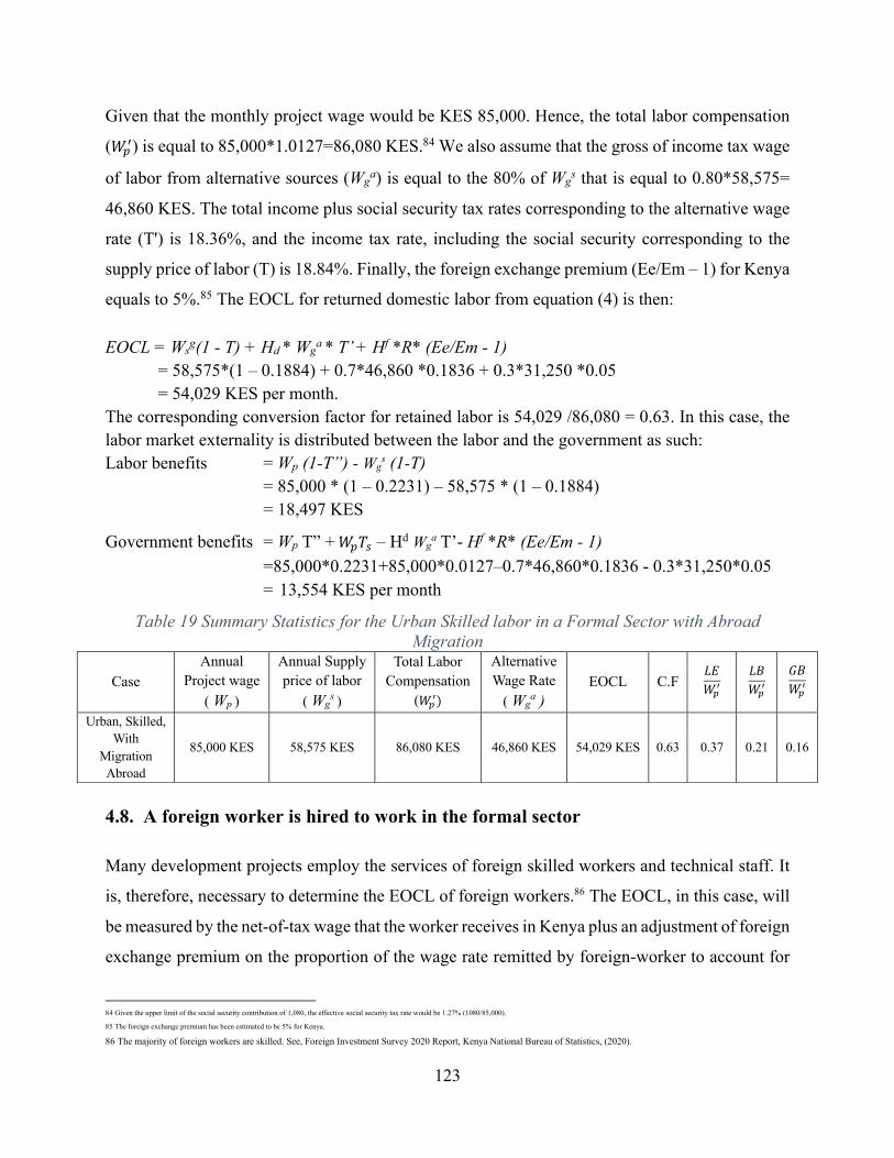
123
Given that the monthly project wage would be KES 85,000. Hence, the total labor compensation
(1GH) is equal to 85,000*1.0127=86,080 KES.84 We also assume that the gross of income tax wage
of labor from alternative sources (Wga) is equal to the 80% of Wgs that is equal to 0.80*58,575=
46,860 KES. The total income plus social security tax rates corresponding to the alternative wage
rate (T') is 18.36%, and the income tax rate, including the social security corresponding to the
supply price of labor (T) is 18.84%. Finally, the foreign exchange premium (Ee/Em – 1) for Kenya
equals to 5%.85 The EOCL for returned domestic labor from equation (4) is then:
EOCL = Wsg(1 - T) + Hd * Wga * T’ + H
f *R* (Ee/Em - 1)
= 58,575*(1 – 0.1884) + 0.7*46,860 *0.1836 + 0.3*31,250 *0.05 = 54,029 KES per month.
The corresponding conversion factor for retained labor is 54,029 /86,080 = 0.63. In this case, the labor market externality is distributed between the labor and the government as such: Labor benefits = Wp (1-T”) - Wg
s (1-T)
= 85,000 * (1 – 0.2231) – 58,575 * (1 – 0.1884) = 18,497 KES
Government benefits = Wp T” +1G+: – Hd Wga T’- Hf
*R* (Ee/Em - 1)
=85,000*0.2231+85,000*0.0127–0.7*46,860*0.1836 - 0.3*31,250*0.05 = 13,554 KES per month
Table 19 Summary Statistics for the Urban Skilled labor in a Formal Sector with Abroad
Migration
4.8. A foreign worker is hired to work in the formal sector
Many development projects employ the services of foreign skilled workers and technical staff. It
is, therefore, necessary to determine the EOCL of foreign workers.86 The EOCL, in this case, will
be measured by the net-of-tax wage that the worker receives in Kenya plus an adjustment of foreign
exchange premium on the proportion of the wage rate remitted by foreign-worker to account for
84 Given the upper limit of the social security contribution of 1,080, the effective social security tax rate would be 1.27% (1080/85,000).
85 The foreign exchange premium has been estimated to be 5% for Kenya.
86 The majority of foreign workers are skilled. See, Foreign Investment Survey 2020 Report, Kenya National Bureau of Statistics, (2020).
Case Annual
Project wage ( Wp )
Annual Supply price of labor
( Wgs )
Total Labor Compensation
())*)
Alternative Wage Rate
( Wga )
EOCL C.F '-))*
'.))*
/.))*
Urban, Skilled, With
Migration Abroad
85,000 KES 58,575 KES 86,080 KES 46,860 KES 54,029 KES 0.63 0.37 0.21 0.16
124
the true cost of the foreign exchange to the economy rather than just its market value. A second
adjustment concerns the goods and services that foreign workers consume in Kenya. If, for
example, they consume subsidized goods and services, the amount of subsidy should be included
in the economic cost of labor. Similarly, if the foreign workers pay any taxes such as the value-
added tax levied on the consumption of foreign workers in the host country, these taxes should be
accounted as an economic benefit to the country and therefore deducted from the cost of foreign
labor.
Algebraically, the economic opportunity cost of foreign labor can be expressed as:
EOCFL = Wf (1 -*.) - W
f (1 – *.)(1 – R) tVAT + W
f (1 – *.) R (Ee / Em - 1) + N (9)
where: • Wf denotes the gross of tax wage of foreign labor;
• *., denotes the personal income tax including the socials security of paid by employee
levied by the host country on foreign labor;
• R denotes the proportion of the net of tax income repatriated by foreign labor;
• Ee/Em-1 denotes the proportion of repatriated income lost via the foreign exchange
premium.
• tVAT denotes the VAT rate levied on consumption; and
• N denotes the value of benefits gained by foreign workers from subsidies.
To estimate the EOCFL in Kenya, we need some additional information. The VAT rate in Kenya
is currently 16%. Assume that foreign workers will need to be paid 146,666 KES (Wp) on a
monthly basis; hence, the income tax rate, including the social security of paid by employees (T/) is 25.54%.87 Also, assume those working abroad will repatriate about one-third of their net of tax
income to their home country. That is, R = 0.33. Also, in this case, we assume that the government
pays no subsidies with respect to these workers, i.e., N = 0.
Applying those values to the equation for EOCL, we estimate the cost to be
87 According to Song, (2016), the income of Chinese migrants is higher than most Kenyans. Nearly one-third of the survey’s participants (32%) had an annual family income
between $8,000 and $16,000, 29% had an income less than $8,000, and 17% were between $16,000 and $32,000. For the purpose of this case, we assume that the annual income of
the foreign worker is USD 16,000.

125
EOCL = Wf (1 - *.) - W
f (1 – *.)(1 – R) tVAT + Wf (1 – *.) R (Ee / Em- 1) + N
= 146,666* (1 - 0.2554) – 146,666*(1 - 0.2554) *(1-0.33) *0.16 + 146,666*(1 - 0.2554) *0.33 * 0.05 + 0
= 99,298 KES per month.
LE = (Wf(1+Ts))-EOCL= 147,746-99,298=48,448 KES per Month.
GB= Wf(*. + *B) + (Wf (1 – *.)(1 – R) tVAT) – (Wf (1 – *.) R (Ee / Em- 1)) - N
= (146,666*0.2627) +( 146,666*(1 - 0.2554) *(1-0.33) *0.16) -(146,666*(1 - 0.2554) *0.33*0.05 + 0).
= 48,448 KES per Month
LB= 0.
Table 20 Summary Statistics for Foreign Labor
In this case, the government accrues the full amount of labor externality caused by using foreign
workers. We are not concerned with the rise in the welfare of the foreign workers in this situation;
thus, any net benefit they gain by migrating to Kenya is not included in an adjustment to the
economic welfare accruing to Kenya because of the project. As previously, we can determine the
conversion factor for foreign labor employed in Kenya. This quantity is 99,298 /147,746 = 0.67.
The rate of government benefit is 0.33.
A summary of all cases investigated in this study is provided in table 9.
Case Monthly
Project wage (Wp)
Monthly Supply price
of labor ( Wg
s )
Total Labor Compensation
())*)
Alternative Wage Rate
( Wga )
EOCL C.F '-))*
'.))*
/.))*
Foreign Labor 146,666 KES --- 147,746 KES --- 99,298 KES 0.67 0.33 0 0.33

126
Table 21 Summary statistics of all cases
Case Project
Location Level of
Skill Source of Workers Distortions !!"
!# Wgs Wg
a EOCL C.F "#!!"
"%!!"
&%!!"
1 Rural
Unskilled
Informal
Sector
Local None 4,474 4,474 4,474 -- 4,474 1 0 -- --
2 Rural
Unskilled
Formal
Sector
Local Social Security 8,049 7,593 7,137 -- 7,137 0.89 0.11 0.00 0.11
2.1 Rural*
Unskilled
Formal
Sector
Local Social Security 9,078 8,564 7,137 -- 7,137 0.79 0.21 0.10 0.11
3 Rural
Skilled
Formal
Sector
Local Income Tax, Social Security 32,493 31,413 31,413 25,130 30,678 0.94 0.06 0.00 0.06
3.1 Rural*
Skilled
Formal
Sector
Local Income Tax, Social Security 38,776 37,696 31,413 25,130 30,678 0.79 0.21 0.115 0.095
4 Urban
Unskilled
Informal
Sector
Local None 8,417 8,417 8,417 -- 8,922 1.06 -0.06 0.00 -0.06
5 Urban
Unskilled
Formal
Sector
Local Social Security 12,530 11,821 11,112 -- 11,779 0.94 0.06 0.00 0.06
6 Urban
Skilled
Formal
Sector
Local Income Tax, Social Security 28,946 27,865 27,865 22,292 27,763 0.94 0.06 0.00 0.06
6.1 Urban*
Skilled
Formal
Sector
Local Income Tax, Social Security 34,518 33,438 27,865 22,292 27,763 0.80 0.20 0.12 0.08
7 Urban
Unskilled
Formal
Sector
Retention
of Out
Migrates
Income Tax, Foreign Exchange, Social
Security 86,080 85,000 58,575 46,860 54,029 0.63 0.37 0.21 0.16
8 Urban
Skilled
Formal
Sector
Foreign Income Tax, Foreign Exchange, Value-
added Tax, Social Security 147,746 146,666 -- -- 99,298 0.67 0.33 0.00 0.33
*, shows the scenario where the project wage (!!) is greater than the supply price of labor (!"#)
127
5. Conclusion
The labor market in Kenya, such as the economy of many low- and middle-income countries, is
characterized by an abundance of labor (labor-surplus economy), especially unskilled labor
(mainly in rural areas), relative to other factors of production. According to different conditions,
it is typical for the economy to manifest differences between nominal wages in the formal and
informal sectors of the economy, as well as seasonal and regional differences in rural and urban
sector wages. These differences highlight the necessity of using the correct cost of labor in applied
cost-benefit analysis.
This study estimated the economic opportunity cost of labor for the Kenya market using the supply
price methodology. This methodology takes the wage offered in the project's labor market area as
the starting point to determine the EOCL. It then adjusts it to account for market distortions and
externalities in that market as well as in other sourcing points for project labor.
Our results revealed that the range of the EOCL in Kenya could range from near equality with the
project wage for unskilled workers to about 63% of the project wage for local skilled labor who
would have migrated abroad. These rates depend heavily on location and the highly differentiated
skills of the labor employed. Most importantly, the wage paid by the project relative to the
minimum wage required (the supply price) to attract sufficient workers with the required skills.
Similarly, the consideration of foreign workers can further enrich these calculations. The preceding
analysis should serve as an operational guide for estimating the EOCL in Kenya.

128
References
Agesa, R. U. (2001). Migration and the urban to rural earnings differences: A sample selection
approach. Economic Development and Cultural Change, 49(4), 847–865.
Agesa, R., & Agesa, J. (2005). Sources of gender difference in rural to urban migration in Kenya:
does human capital matter? Applied Economics Letters, 12(11), 705–709.
Brauw, A. De, Mueller, V., & Lee, H. (2014). The role of rural-urban migration in the structural
transformation of Sub-Saharan Africa. World Development.
EY. (2021). Worldwide Personal Tax and Immigration Guide.
Harberger, A. C. (1972). On Measuring the Social Opportunity Cost of Labour. In Project
Evaluation (pp. 157–183). Palgrave Macmillan UK.
Harberger, A. C. (1985). Reflections on Social Project Evaluation. In Pioneers in development, 2.
International Labour Organization. (n.d.). IILOSTAT database. Data were retrieved on January
29, 2021.
Jenkins, G. (1995). Economic Opportunity Cost of Labor: A Synthesis. Cambridge, MA: Harvard
Institute for International Development, Harvard Un.
Jenkins, G., Kuo, C., & Harberger, A. (2019). Cost-Benefit Analysis for Investment Decisions: Chapter 12 (The Economic Opportunity Cost of Labor).
Mott, F., & Shapiro, D. (1984). Seasonal variations in labor-force activity and intrahousehold
substitution of labor in rural Kenya. The Journal of Developing Areas, 18(4), 449–464.
Mwangi, T., Simiyu, F., & Beyene, L. (2017). The effects of minimum wages on the labor market
and income distribution in Kenya: A CGE analysis. Partnership for Economic.
Oyvat, C., & Gĩthĩnji, M. wa. (2020). Migration in Kenya: beyond Harris-Todaro. International
Review of Applied Economics, 34(1), 4–35.
Ratha, D. (2011). Leveraging Migration for Africa: Remittances, skills, and investments.

129
Song, D. (2016). Chinese Migrant Workers in Kenya: Their Health Status and Access to Health
Care.
Wambugu, A., Christopher, A., Collier, P., & Ndung’u, N. (2010). Kenyan Labour Market
Challenges. Policies for Prosperity., Cambridge, UK: Oxford University Press, Collections.
College of Humanities and Social Sciences (CHSS), 267-292.
World Bank. (2020). Inflows: Annual Remittances Data.
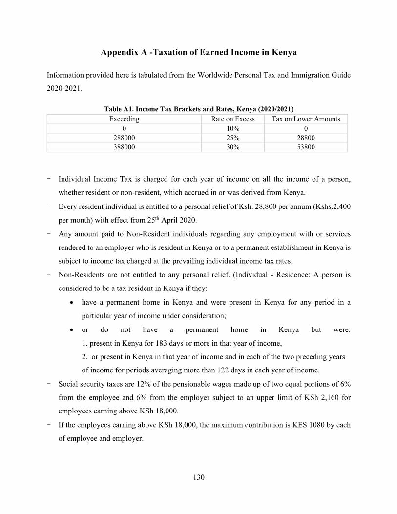
130
Appendix A -Taxation of Earned Income in Kenya
Information provided here is tabulated from the Worldwide Personal Tax and Immigration Guide
2020-2021.
Table A1. Income Tax Brackets and Rates, Kenya (2020/2021) Exceeding Rate on Excess Tax on Lower Amounts
0 10% 0 288000 25% 28800 388000 30% 53800
- Individual Income Tax is charged for each year of income on all the income of a person,
whether resident or non-resident, which accrued in or was derived from Kenya.
- Every resident individual is entitled to a personal relief of Ksh. 28,800 per annum (Kshs.2,400
per month) with effect from 25th April 2020.
- Any amount paid to Non-Resident individuals regarding any employment with or services
rendered to an employer who is resident in Kenya or to a permanent establishment in Kenya is
subject to income tax charged at the prevailing individual income tax rates.
- Non-Residents are not entitled to any personal relief. (Individual - Residence: A person is
considered to be a tax resident in Kenya if they:
• have a permanent home in Kenya and were present in Kenya for any period in a
particular year of income under consideration;
• or do not have a permanent home in Kenya but were:
1. present in Kenya for 183 days or more in that year of income,
2. or present in Kenya in that year of income and in each of the two preceding years
of income for periods averaging more than 122 days in each year of income.
- Social security taxes are 12% of the pensionable wages made up of two equal portions of 6%
from the employee and 6% from the employer subject to an upper limit of KSh 2,160 for
employees earning above KSh 18,000.
- If the employees earning above KSh 18,000, the maximum contribution is KES 1080 by each
of employee and employer.
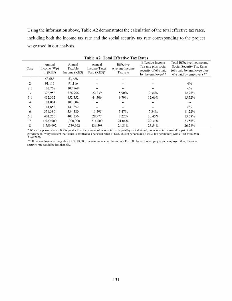
131
Using the information above, Table A2 demonstrates the calculation of the total effective tax rates,
including both the income tax rate and the social security tax rate corresponding to the project
wage used in our analysis.
Table A2. Total Effective Tax Rates
Case Annual
Income (Wp) in (KES)
Annual Taxable
Income (KES)
Annual Income Taxes Paid (KES)*
Effective Average Income
Tax rate
Effective Income Tax rate plus social security of 6% paid by the employee**
Total Effective Income and Social Security Tax Rates
(6% paid by employee plus 6% paid by employer) **
1 53,688 53,688 -- -- -- -- 2 91,116 91,116 -- -- -- 6%
2.1 102,768 102,768 -- -- -- 6% 3 376,956 376,956 22,239 5.90% 9.34% 12.78%
3.1 452,352 452,352 44,306 9.79% 12.66% 15.52% 4 101,004 101,004 -- -- -- -- 5 141,852 141,852 -- -- -- 6% 6 334,380 334,380 11,595 3.47% 7.34% 11.22%
6.1 401,256 401,256 28,977 7.22% 10.45% 13.68% 7 1,020,000 1,020,000 214,600 21.04% 22.31% 23.58% 8 1,759,992 1,759,992 436,598 24.81% 25.54% 26.28%
* When the personal tax relief is greater than the amount of income tax to be paid by an individual, no income taxes would be paid to the government. Every resident individual is entitled to a personal relief of Ksh. 28,800 per annum (Kshs.2,400 per month) with effect from 25th April 2020 ** If the employees earning above KSh 18,000, the maximum contribution is KES 1080 by each of employee and employer; thus, the social security rate would be less than 6%.

[This page is intentionally left blank]

133
Annexure D: Social Value of Time

134
Estimation of National Parameters and Development of Project Case Studies for Investment Project Appraisal Social Value of Time Report
Date: September 29, 2021 Submitted by: Cambridge Resources International, Inc. 1770Mass.Ave#617,Cambridge,MA02140,USA Phone: 1 (613) 770 2080 E-mail: [email protected] or [email protected]
In Consortium with: GEEKAN KENYA LTD RUPRANI HOUSE, MOKTAR DADAH P.O BOX 17460-00100 TEL:+254723729096 Email: [email protected] NAIROBI-KENYA. Presented to: THE MINISTRY OF NATIONAL TREASURY AND PLANNING, KENYA

135
Summary
In this manual, the social value of time (SVT) is estimated for evaluating public investments
in three public sectors of Kenya: transportation, water and sanitation, and public office services.
Improving the quality of and access to services in these sectors can potentially result in time
savings for households and firms. Table 1 summarizes the estimated economic values of time
savings in 2019 prices (the latest year for which public data was available at the time of this
analysis), both in Kenyan Shillings (KES) and the United States Dollars (USD).
Panel A reports the monetary value of times savings for transportation projects in urban and
rural regions per passenger and by vehicle modes. The results indicate that the time saved for
truck drivers has the highest value in both urban and rural areas (115.50 and 26.94 KES per
hour, respectively). However, the collective value of time savings by passenger occupancy
appears to be the highest for public transportation modes, i.e., buses (1,461.02 and 340.78 KES
per hour, respectively).
Table 22: Summary of estimated SVTs for Kenya by sector and by beneficiaries
Project's sector and beneficiaries The monetary value of time savings
(2019 prices) KES per hour USD per hour
Panel A. Transportation projects
a. Per passenger Urban
Light vehicles (cars & motorcycles) 66.41 0.66 Buses 54.11 0.54 Trucks 115.50 1.14
Rural Light vehicles (cars & motorcycles) 15.49 0.15 Buses 12.62 0.12 Trucks 26.94 0.27
b. Per vehicle
Urban Light vehicles (cars & motorcycles) 132.83 1.32 Buses 1,461.02 14.47 Trucks 115.50 1.14
Rural Light vehicles (cars & motorcycles) 30.98 0.31 Buses 340.78 3.37 Trucks 26.94 0.27
Panel B. Water and sanitation projects Adults
Lower bound 21.37 0.21 Upper bound 35.61 0.35
Children Lower bound 10.68 0.11 Upper bound 17.81 0.18
Panel C. Delivery of public services Personal
Lower bound 21.37 0.21 Upper bound 35.61 0.35
Commercial 115.50 1.14

136
In Panel B, the monetary value of travel time reductions resulting from water and sanitation
projects are reported for adults and children in Kenya. The estimated values indicate that an
hour reduction in the time spent to fetch drinking water or access sanitation facilities can lead
to time savings in the ranges of 21.37 to 35.61 KES (0.21 to 0.35 USD) and 10.68 to 17.81
KES (0.11 and 0.18 USD) for adults and children, respectively.
Panel C shows the economic benefits of time savings due to improving the efficiency of public
service deliveries. The realized benefits will be substantial regardless of whether the purpose
of visiting public offices is personal (e.g., medical treatments at public clinics or hospitals,
applying for passports or driver's licenses, etc.) or commercial (e.g., renewing business permit
or registering commercial motor vehicles). For personal visits, an hour reduction in the duration
of service delivery has an approximate monetary value between 21.37 and 35.61 KES (0.21
and 0.35 USD). Given the higher opportunity cost of time among those visiting public offices
for commercial purposes, the economic value of time-saving can be up to 115.50 KES (1.14
USD) per hour for them.
137
1. Introduction
There are many instances where public sector projects can potentially lead to time savings for citizens and firms in a country. Such projects either facilitate better utilization of existing capital stocks (e.g., road improvement projects and projects reducing the time required to obtain public services) or provide public services to areas without access to those services (e.g., water supply and sanitation projects). Therefore, estimating the social value of time (SVT) is crucial when planning agencies conduct investment appraisals to assess the optimality of the existing situation versus the economic feasibility of potential improvements.
Given that individuals can reallocate time savings to other welfare-improving activities, the social value of time saved by a project adds up to the project's total benefits. The social value of time is made up of two components: the resource value of time, which can be traded off with income (the value of working time saved), and the value of the utility derived from the time that now can be spent on other income- or non-income-generating activities. The first component corresponds to the value of time saved by those individuals who will allocate marginal savings in time to their occupation. The second component reflects the value that individuals place on adjustments of consumption patterns or modifications to their schedule of activities.
With diverse preferences among individuals in a society, it is expected that the social value of time savings ranges from as high as the prevailing market wages to as low as zero. For instance, taxi drivers, truck drivers, and traveling sales personnel will be more productive over their active working hours if they can travel at a higher average speed on the road. Or similarly, people may be spending several minutes or hours of their active working time queuing up to pay their annual road tax or to carry out banking activities. For this group of individuals, the net impact of an intervention that reduces waiting times can potentially translate into more productive working hours88.
On the opposite extreme, there are some individuals whose supply price of time in a given activity is essentially zero: children on a road trip, infants accompanying their parents, women socializing with other women in their community while fetching drinking water from remote sources, or retired people enjoying the opportunity to go for a drive or to socialize with friends while waiting in a queue. In each case, the supply price of time for such activities might be very low or zero.
Between these two extremes, there is a distribution of the social value of time for individuals with an array of opportunity costs. The social value of time for this group of individuals is greater than zero but less than the market wage. Thus, the expected social value of time saved by an intervention (the expected benefit) should be estimated as a weighted average of the social value of time for these three groups.
Figure 1 illustrates the distribution of social value to time per hour time-saving for three groups. The first group (denoted by α) are those individuals who become more productive during
88 It should be notified here that there are also some exceptions where the changes in a households’ time allocation caused by a public sector intervention turns to be negative (i.e., a cost to the household). For example, the development of a hydro dam project may displace some households, forcing them to relocate farther away from their work or school. As a consequence, they may spend more time commuting. In this case the change in time allocation would decrease individuals’ well‐being and should be counted as a cost of the intervention.
138
working hours due to the project implementation. This group's economic value per hour of time-saving equals the average market wage rate (w). The next group (denoted by β) consists of those individuals with an opportunity cost less than the market wage rate but greater than zero. And individuals in the third group (denoted by μ), perhaps a small proportion of project beneficiaries, have a zero opportunity cost.
Figure 12: Distribution of economic value of time
An intervention's weighted average social value of an hour saved (or lost for projects with displacements) equals the area "0wABC" in Figure 1. Equation 1 represents the mathematical formulation of this area with three components,
SVT = α ×(SVT! = w) + β ×SVT" + µ(SVT# = 0) (1)
where, SVTα, SVTβ, and SVTμ represent the social value of time to proportions α, β, and μ, respectively. The first component captures the rectangle 0wAD, the product of α, and the average market wage rate. The area of triangle ABD represents the second component, the value of time to those with opportunity costs greater than zero but less than the average market rate. Here, we assume that the distribution between w and zero is linear, as shown by the solid line AB. So, the area of triangle ABD is equal to 0.5×w. The calculated value for area ABD would be different if our assumption regarding the distribution of values changes; a higher value will arise if the curve AB is concave to the origin and a lower value if the curve AB is convex (the dashed lines in Figure 1). Lastly, the third component of Eq. 1 captures the proportion of time savings without any social value.
The following sections will discuss how the methodology described above can be applied to investment appraisals in Kenya when estimating the social value of time for public sector projects. For this purpose, we review case studies with representative data for three sectors: transportation, water and sanitation, and public services.

139
2. Social Value of Time in Transportation Projects
2.1 Estimating Social Value of Time for Rural and Urban Vehicle Occupants Our approach for estimating the social value of time is based on the opportunity cost of time for different road users. The rationale behind this approach is that individuals will value the time savings according to their opportunities for reallocation of the time savings to other activities. For some people, travel time is a component of their work time and, therefore, they have the opportunity to trade it off with more productive working hours. As a result, the opportunity cost of time sacrificed in traffic equals their hourly wage rate. But, this is not necessarily the case for all people on the road. That is why the first step of estimating the SVT for vehicle modes is to figure out the distribution of road users based on their opportunity costs of time. In the absence of data from surveys to ascertain the distribution of the opportunity costs, we assume that the distribution is similar to the distribution illustrated in Figure 1.
Additionally, we know that the opportunity cost of time saved is different for vehicle modes carrying various travelers. Hence, we begin with the information available on vehicle modes in Kenya, broadly categorized as light vehicles (cars and motorcycles), buses, and trucks. As shown in Table 2, by the end of 2019, 3.61 million vehicles were registered by the National Transport and Safety Authority (NTSA). Out of the total population of vehicles on the road, 78 percent (2.81 million) were light vehicles, 3 percent (0.11 million) were buses, and 19 percent (0.69 million) were trucks.
Table 23: Distribution of total distance traveled by vehicle modes in Kenya in 2019
Vehicle mode
Vehicle population
(mil. vehicles)
Distance traveled
(mil. km)
Distance traveled by occupants
(mil. km)
(1) (2) (3)
(1) Light vehicles (motorcycles & cars) 2.81 24,100 48,200
(2) Buses 0.11 2,728 73,656
(3) Trucks 0.69 34,230 34,230
(4) Total 3.61 61,058 156,086
Source: Vehicle population and types from Kenya Association of Manufacturers, KAM (2020); Annual gasoline and diesel consumption from Kenya's Energy and Petroleum Regulatory Authority, EPRA (2020).
When evaluating a transportation project, the economic value of time savings by road users should be taken into account. The methodology described in Section 1 and illustrated in Figure 1 can be used for this purpose. The first step is to estimate the proportion of distance traveled by vehicle passengers for work purposes (valued at w), non-work purposes with some value (less than w but greater than zero), and non-work purposes with zero value. So, we begin with the information about the total annual fuel consumption in Kenya that enables us to calculate the total kilometers driven in Kenya by all vehicle modes.

140
According to the 2020 annual report of Kenya's Energy and Petroleum Regulatory Authority (EPRA), total gasoline and diesel consumption amounted to 1,687 and 2,587 million liters in 2019, respectively. Therefore, assuming an average fuel efficiency of 100 km per 7 liters for the vehicle fleet, we can estimate how many kilometers were approximately driven by light vehicles (gasoline-engine) and buses and trucks (diesel-engine) in 2019. For light vehicles, the calculation is straightforward: 1,687 million liters of gasoline consumed by 2.81 million vehicles, each having an average fuel efficiency of 100 km per 7 liters. So, the total distance traveled by light vehicles (Table 2, row 1, column 2) can be estimated as:
Total distance traveled = ((100 km)/ (7 liters)) × 1,687 mil. liters = 24,100 mil. km
For buses and trucks, the total amount of diesel consumed in 2019 is 2,587 million liters, and therefore, the total distance traveled by diesel-engine vehicles can be estimated as:
Total distance traveled = ((100 km)/ (7 liters)) × 2,587 mil. liters = 36,958 mil. km
The 36,958 million kilometers traveled by diesel-engine vehicles include the distance traveled by both buses and trucks. To determine the total kilometers traveled by each, we need the relative frequency of road travel by buses to trucks. We assume that the average number of kilometers driven by an average truck is approximately two times as many kilometers as an average minibus or bus. Therefore, denoting X as the number of kilometers traveled by buses and 2X by trucks, we will have:
(0.11 mil. vehicles× X) + (0.69 mil. vehicles × 2 × X) = 36,958 mil. km
1.49X = 36,957
X=24,804 km/vehicle
So, the total distance traveled by buses and trucks (Table 2, rows 2 and 3, column 2) is 2,728 and 34,230 million kilometers, respectively (see below).
Total distance traveled by buses=0.11 mil. vehicle × 24,803 km/vehicle = 2,728 million km
Total distance travelled by trucks=0.69 mil. vehicle×2×24,803 km/vehicle = 34,230 million km
To estimate the total distance traveled by occupants (Table 2, column 3), we need the number of passengers associated with the utilization of each vehicle mode. Here, we assume that, on average, each car carries two people (driver plus one passenger), each bus 27 people (one driver plus 26 passengers), and each truck one driver89. Then, we multiply the average number of
89 There are on average 14 seats in minibuses and 40 seats in larger buses. So, we assume an average of 27 seats for minibuses and buses combined.
141
passengers by the total distance traveled by each vehicle mode. As shown in Table 2, column 3, the results indicate that 156,086 million occupant-kilometers were traveled on the Kenyan roads in 2019, made up of 48,200, 73,656, and 34,230 million occupant kilometers of travel by light vehicles, buses, and trucks, respectively.
Tables 3 and 4 show the estimated parameter values for α, β, μ, the average social value of time per hour by vehicle type for urban (Table 3) and rural road users (Table 4). The following assumptions are made for the proportion of distance traveled by each mode's occupants for work purposes: 25 percent for light vehicles, 0.04 percent (1 driver out of 27 bus occupants, 1/27) for buses, and 100 percent for trucks. Assuming 10 percent of the people traveling by buses and light vehicles put a zero value on their travel time (μ = 0.10), the proportion β is equal to 0.65, 0.86, and 0 for occupants of light vehicles, buses, and trucks, respectively (column 3 in Tables 3 and 4). Figure 2 shows the distribution of the social value of time by vehicle modes.
Once the values of α, β, and μ are set, we use Equation 1 to estimate the weighted average social value of time for each mode:
SVT!"#$%'($")*(+ = (0.25 × w) + (0.65 × 0.5 × w) + (0.10 × 0) = 0.58w (2)
SVT,-+(+ = (0.04 × w) + (0.86 × 0.5 × w) + (0.10 × 0) = 0.47w (3)
SVT./-)0+ = (w) + (0 × 0.5 × w) + (0.10 × 0) = w (4)
The weighted average SVT for each mode is a fraction of the average hourly wage (w). We use the minimum wage in urban and rural areas to approximate the average hourly wage rate. According to the Regulation of Wages Order in Kenya, the hourly wage is 115.50 KES/hour in urban regions of Kenya. The average social value of time per passenger per hour traveling by light vehicles, buses, and trucks is estimated to be 66.41 KES (0.66 USD), 54.11 KES (0.54 USD), and 115.50 (1.14 USD), respectively (Table 3, columns 6 and 7).
These estimated SVTs are for representative passengers in different vehicle modes, not for the vehicle modes themselves. When appraising road investment projects, the economic benefits of time savings are assessed by comparing travel time without- and with-project for different vehicle modes. Thus, we should break down the estimates of representative passengers for vehicle modes by multiplying the number of passengers in each vehicle mode by the corresponding SVT per hour per passenger. The SVT per hour for light vehicles (2 passengers), buses (27 passengers), and trucks (1 passenger) are 132.83 KES (1.32 USD), 1,461.02 KES (14.47 USD), and 115.50 KES (1.14 USD), respectively (Table 3, columns 8 and 9).
We repeat the same exercise for rural regions, assuming that the parameter values for α, β, and μ are identical across urban and rural areas (Table 4, columns 2 - 4). The only difference in SVT estimation for rural households is that the average hourly wage is less in rural than urban regions. The minimum wage is regulated for rural workers at 269.40 KES per day, 26.94 KES/hour assuming a 10-hour working day. In rural areas of Kenya, the average SVT per passenger per hour traveling by light vehicles, buses, and trucks is 15.49 KES (0.15 USD), 12.62 KES (0.12 USD), and 26.94 KES (0.27 USD), respectively (Table 4, columns 6 and 7). Lastly, we estimate the SVT values by vehicle modes: 30.98 KES (0.31 USD), 340.78 KES (3.37 USD), and 26.94 KES (0.27 USD) per hour for light vehicles, buses, and trucks, respectively (Table 4, columns 8 and 9).

142
Table 24: Estimation of Average SVT for Urban Travelers
Vehicle mode
Distance traveled by vehicle occupants
% of total*
Travel purpose and value Weighted average
SVT, % of wage (w)
SVT per hour per
passenger (KES)
SVT per hour per
passenger (USD)**
SVT per hour per vehicle (KES)
SVT per hour per vehicle (USD)
Work (α)
Non-work and non-
zero (β)
Non-work and zero
(μ)
(1) (2) (3) (4) (5) (6) (7) (8) (9)
(1) Light vehicles 0.31 0.25 0.65 0.10 0.58 66.41 0.66 132.83 1.32
(2) Buses 0.47 0.04 0.86 0.10 0.47 54.11 0.54 1,461.02 14.47
(3 ) Trucks 0.22 1.00 0 0 1.00 115.50 1.14 115.50 1.14
Notes: * values in column 1 are estimated by dividing the distance travelled by each vehicle mode occupants (Table 1, column 3, rows 1-3) by total distance travelled by all vehicle occupants combined (Table 1, column 3, row 4). * an exchange rate of 101 KES/USD is used to convert KES to USD.
143
Table 25: Estimation of Average SVT for Rural Travelers
Vehicle mode
Distance travelled by vehicle occupants, % of total
Travel purpose and value Weighted average
SVT, % of wage (w)
SVT per hour per
passenger (KES)
SVT per hour per
passenger (USD)
SVT per hour per vehicle (KES)
SVT per hour per vehicle (USD)
Work
(α)
Non-work and non-zero
(β)
Non-work and zero
(μ)
(1) (2) (3) (4) (5) (6) (7) (8) (9)
(1) Light vehicles 0.31 0.25 0.65 0.10 0.58 15.49 0.15 30.98 0.31
(2) Buses 0.47 0.04 0.86 0.10 0.47 12.62 0.12 340.78 3.37
(3 ) Trucks 0.22 1.00 0 0 1.00 26.94 0.27 26.94 0.27
Notes: * values in column 1 are estimated by dividing the distance travelled by each vehicle mode occupants (Table 1, column 3, rows 1-3) by total distance travelled by all vehicle occupants combined (Table 1, column 3, row 4). * an exchange rate of 101 KES/USD is used to convert KES to USD.

144
Panel A: Light Vehicles
Panel B: Buses
Panel C: Trucks
Figure 13: Distribution of social value of time by vehicle modes
2.2 Projecting the SVT over the Project's Evaluation Period
The economic value of travel time savings over the project's lifetime is often a significant benefit in appraising transportation projects. Hence, we need to project the social value of time

145
estimates by an assumed path of growth over future periods. For this purpose, one has to adjust the real value of time savings in every particular year by the expected growth rate in real wages in that year. As real wages grow, the value of time savings grows as well. The growth rate in real wages in a country is often assumed to be approximately equal to the country's growth rate in real GDP per capita. Therefore, we need to build an index for real wage growth over time to adjust the future SVT values, as shown in Equation 5.
Real Wage Growth (RWG) indext = RWG indexb × (1 + RWG rate)t - b (5)
RWG indext is the real wage growth index in period t, RWG indexb is the real wage growth index in the base period (b), and the RWG rate is the expected growth rate in GDP per capita. The value of the index in the base period, RWG indexb, is always set to 1 for normalization purposes. This normalization facilitates a consistent comparison of monetary values across current and future periods during the project lifetime.
Let us now look at an example to see how we can use our estimated SVT in the previous section and Eq. 5 to project SVT over the lifespan of a project. Suppose we want to evaluate the economic feasibility of a transportation project that starts in 2019 (the base year) and has a 10-year evaluation period. For simplicity, we assume that the social value of time for road users is equal to the average of the estimated SVT for all vehicle modes in column 6 of Tables 3 and 4: 78.67 KES per hour per passenger for an urban traveler and 18.35 KES per hour per passenger for a rural traveler.
The first step in projecting these economic benefits into future periods (2020 through 2028) is to determine the expected growth rate for real wages in Kenya over the project's lifetime. According to the IMF economic outlook database, Kenya's real GDP per capita has grown on average by 3.40 percent per annum from 2010 through 2019. We assume that Kenya's real GDP per capita grows at the same rate per annum over the project's lifetime. Then, using Eq. 5, we construct the real wage growth index (Table 5, row 2). Once the RWG index is built for the whole evaluation period, we can use it to project the SVT estimates for urban and rural travelers. For a specific year, we have to multiply the SVT in the base period by the RWG index of that year. For instance, the projected SVT per hour for urban travelers in 2024 is 92.99 KES, i.e., 78.67 × 1.18.
Table 26: Projection of SVT for Urban and Rural Travelers, base year = 2019
Year 2019 2020 2021 2022 2023 2024 2025 2026 2027 2028
(1) Years passed from the base year* 0 1 2 3 4 5 6 7 8 9
(2) Real wage growth index** 1.00 1.03 1.07 1.11 1.14 1.18 1.22 1.26 1.31 1.35
(3) SVT (KES per hour – Urban) 79 81 84 87 90 93 96 99 103 106
(4) SVT (KES per hour – Rural ) 18 19 20 20 21 22 22 23 24 25
Notes: * denotes that row 1 shows the value of (t – b) in Eq. 3. ** represents that the real wage growth index is calculated using Eq. 3: (1+0.0340)t-b
146
Table 6 repeats the same exercise using the estimated SVT values by vehicle modes (column 8 in Tables 2 and 3). As mentioned before, reporting SVT values by vehicle modes is helpful since most transportation projects measure costs and benefits by vehicle modes, not passengers.
Table 27: Projection of SVT for urban and rural travelers by vehicle modes (base year:
2019)
The projected SVTs for urban and rural regions reflect the average magnitude of the welfare improvement of passengers traveling by each mode. This welfare improvement comes about through increased productivity during working hours, or increased utility individuals enjoy due to a one-hour reduction in travel time. Therefore, the present value of these time savings over the project's lifetime should be added to the present value of other expected benefits from improvements (such as savings in vehicle operating costs) when evaluating the economic feasibility of a transportation (or transportation-related) project.
2.3 Estimation of the SVT for Projects Starting in a Future Period
In the previous, we used an example to show how the estimated SVT values in the base year are projected over the lifespan of a project. The assumption was that the project was designed to come to service in 2019, the same year for which SVT values were estimated. However, in some cases, project appraisal needs to be conducted for projects starting in a future period. Therefore, the estimated SVT values for the base year (2019 in our example) must be adjusted before projections by the RWG index. For instance, suppose that our example project comes to service in 2026 instead of 2019. If so, the project analyst has to rebase the estimated SVT values from 2019 to 2026 before projecting the SVT values for future periods.
Rebasing is done by multiplying the estimated value of the existing base year by the ratio of nominal GDP per capita of the new base year (n) to nominal GDP per capita of the current base year (b), as shown in Eq. 6:
SVTn=SVTb×
Nominal GDP per capitanNominal GDP per capitab
(6)
Year 2017 2018 2019 2020 2021 2022 2023 2024 2025 2026
(1) Real wage growth index 1.00 1.03 1.07 1.11 1.14 1.18 1.22 1.26 1.31 1.35
Urban
(2) Light vehicles 133 137 142 147 152 157 162 168 174 179
(3) Buses 1461 1511 1562 1615 1670 1727 1786 1846 1909 1974
(4) Trucks 116 119 123 128 132 137 141 146 151 156
Rural
(5) Light vehicles 31 32 33 34 35 37 38 39 40 42
(6) Buses 341 352 364 377 390 403 416 431 445 460
(7) Trucks 27 28 29 30 31 32 33 34 35 36

147
In our example, we need the nominal GDP per capita of Kenya in 2019 and 2026. According to the IMF economic outlook database, the realized nominal GDP per capita in 2019 (listed as GDP per capita current local currency in the IMF data) is 204,629 KES, and the forecasted nominal GDP per capita in 2026 is 361,896 KES. Using this data, we rebase our estimated SVT values from 2019 to 2026.
SVT!"!#=SVT2019×
Nominal GDP per capita2026Nominal GDP per capita2019
(7)
For instance, the SVTs per hour per vehicle for light vehicles in urban and rural regions in 2026 are shown in Equations 8 and 9, respectively:
Urban:Lightvehicles-SVT2026=133×
361,896204,629
=235BCDEFGℎIJG(8)
Rural:Lightvehicles-SVT2026=31×
361,896204,629
=55KESperhour(9)
Following the same method, we rebase the SVT estimates for other vehicle modes (see Table 7).
Table 28: Rebasing the estimated SVT values from 2019 to 2026
Vehicle mode Urban: SVT per hour per vehicle
(KES) Rural: SVT per hour per vehicle
(KES) 2019 2026 2019 2026
(1) Light vehicles 133 235 31 55 (2) Buses 1461 2584 341 603 (3) Trucks 116 204 27 48
Once the SVT values are estimated at 2026 prices, projections can be made into the future periods, as described in Table 6. Similarly, we consider a 10-year evaluation period from 2026 to 2035. The real wage growth index is constructed using Eq. 5, with the real wage growth rate estimated by averaging growth rate forecasts in GDP per capita from 2021 to 2026. Table 8 reports the SVT estimates at 2026 prices by vehicle mode and rural/urban status.
Table 29: Projection of SVT for urban and rural travelers by vehicle modes (base year:
2026)
Year 2026 2027 2028 2029 2030 2031 2032 2033 2034 2035
(1) Real wage growth index 1.00 1.03 1.05 1.08 1.11 1.14 1.17 1.20 1.24 1.27
Urban
(2) Light vehicles 235 241 248 254 261 268 275 283 290 298
(3) Buses 2,584 2,653 2,724 2,797 2,872 2,950 3,029 3,110 3,193 3,279
(4) Trucks 204 210 215 221 227 233 239 246 252 259
Rural
(5) Light vehicles 55 56 58 59 61 63 64 66 68 70
(6) Buses 603 619 635 652 670 688 706 725 745 765
(7) Trucks 48 49 50 52 53 54 56 57 59 60

148
3. Social Value of Time in Water and Sanitation Projects
3.1 Estimating the SVT for the Base Period
This section reviews the current provision of water and sanitation services across Kenya and estimates the social value of time savings if improvements are implemented in providing such services. Similar to the transportation sector projects, the time savings from improved access to water and sanitation services can result in increased productivity or increased utility individuals enjoy due to reallocating the saved time to other welfare-improving activities such as leisure and child-care.
As of 2015 (the latest publicly available dataset at the time of this report), twenty-nine percent of Kenya's population did not have access to improved drinking water sources (MIS, 2015)90. The distribution of drinking water sources by locality reveals that the majority of the households without improved drinking water sources are rural households: 38 percent of the rural population compared to 12 percent of the urban population (Table 9).
Table 30: Distribution of households in Kenya by the source of drinking water
Characteristic Kenya Urban Rural Source of drinking water
Improved 71% 88% 62% Unimproved 29% 12% 38%
Time to obtain drinking water (round trip) Have water on premises 41% 67% 41% Less than 30 minutes 32% 20% 32% 30 minutes or longer 27% 13% 27% Source: 2015 Malaria Indicator Survey (MIS) Report
Moreover, fifty-nine percent of Kenyan households had to spend some time during the day to obtain drinking water. In urban regions, 20 percent of the population spends up to 30 minutes, 13 percent at least 30 minutes or longer to fetch drinking water. Bringing drinking water takes even longer for rural households: 32 percent spend up to 30 minutes, and 27 percent at least 30 minutes or longer.
Similarly, it is common that households have to spend a substantial amount of time accessing sanitation facilities. As shown in Table 10, seventy percent of Kenyan households use unimproved toilet facilities or open defecation (no facility)91. Slicing up the population by
90 Improved sources of drinking water include piped water into own/neighbor dwelling, public tap, borehole, protected dug well and bottled water. Unimproved sources include unprotected dug well, unprotected spring, tanker truck and surface water. 91 A household is classified as having access to improved facility if the facility is used only by members of one households. Different types of improved facility include: flush to piped sewer/septic tank/pit latrine, ventilated improved pit (VIP) latrine, pit latrine with a slab or composting toilet. An unimproved facility can be either a shared facility (would be an improved facility if not shared with other households) or a facility with flush not to sewer/septic tank/pit latrine, pit latrine without slab/open pit, bucket, or hanging toilet/latrine.
149
locality, we observe that shared toilets emerge as the typical unimproved facility in urban regions (38 percent). In contrast, unimproved facilities such as pit latrines without slab/open pit are mainly the type of facility to which rural households have access (46 percent). Open defecation is more common among the rural population (14 percent) than the urban population (3 percent). The MIS survey does not report the time spent by individuals to reach sanitation facilities. Still, households without sanitation facilities at their premises may spend 30 minutes or longer of their time during the day to access sanitation facilities.
Table 31: Distribution of households by type of and time to sanitation facilities
Household Characteristics Kenya Urban Rural Type of facility
Improved source, not shared 30% 36% 25% Unimproved
Shared facility* 23% 38% 15% Unimproved facility 36% 23% 46%
No facility (open defecation) 11% 3% 14%
Time to reach a facility Open defecation 21% 8% 34% In own dwelling 38% 51% 24% Less than 30 minutes 31% 29% 33% More than 30 minutes 10% 11% 9% Source: 2015 Malaria Indicator Survey (MIS) Report Notes: * denotes that these facilities would be considered improved if two or more households did not share them.
The statistics described in Tables 9 and 10 imply that improving access to water and sanitation services generates non-health benefits, in the form of time savings, in addition to health benefits. Hence, the economic value of time savings from the society's perspective has to be considered by the project analyst when appraising projects in the water and sanitation sector.
A standard approach to estimate the economic value of time savings due to improved access to water and sanitation facilities is to conduct surveys to collect individual-level information about household's needs and preferences. Such detailed surveys provide us with the distribution of households' opportunity costs of time. In the absence of such data, however, the project analyst can use community- or regional-level data to approximate the distribution of representative households' time preferences and the monetary value of the time savings. Similarly, the analyst can rely on the existing studies in the literature. Table 11 summarizes the assumptions made by previous cost-benefit analyses on the monetary value of time savings due to improved access to water and sanitation services.
The monetary values assigned to time savings range from 30 percent to 50 percent of the average wage rate (or minimum wage in some cases) for adults and 15 percent of the average wage rate for children 15 years old or younger. Following the existing literature, we assume the following lower and upper bounds for the value of time savings after improvements in water and sanitation services in Kenya: 30 and 50 percent of the hourly wage rate for adults, and 25 and 15 percent of the hourly wage rate for children, respectively.

150
We use the same minimum wage figures that we used in Section 2 for transportation projects for the average wage rate values. According to the minimum wage laws in Kenya, the hourly wage for urban households is 115.50 KES/hour, whereas the hourly wage for rural workers is 26.94 KES/hour.

151
Table 32: Assumptions made by existing studies for the value of time savings due to water supply and sanitation interventions
Reference Source Location of study The monetary value of time savings Time savings as a percentage of the
total benefits
Whittington et al. (2009) Foundations and Trends in Microeconomics
Low-income countries 30% of the daily wage rate 15 %
Whittington et al. (2012) World Development Developing countries 30% of the daily wage rate 15 %
Hutton et al. (2015) World Bank Water and Sanitation Program
South Asia 30% of wage for adults and 15 % for children ≤ 15 50 %
Hutton (2015) Copenhagen Consensus Center Global 30% of wage for adults and 15 % for children ≤ 15 70 %
Cook et al. (2016) Water Resources Research Kenya 50% unskilled wage rate
NA
Whittington et al. (2017) Copenhagen Consensus Center Haiti 50% of the daily wage rate 33 %
Larsen (2018) Copenhagen Consensus Center India 50% of the daily wage rate for people > 5 40 – 60 %
Hutton (2018) UNICEF India • Household questionnaire for income-earning adults to
estimate daily earnings • Minimum wage rate in rural areas for non-income
earning adults • 50% of minimum wage for school-age children • no value given to the time of children ≤ 5 years
NA

152
Table 12 shows the estimated values vary across urban and rural regions. The value of an hour saved by urban adults ranges between 34.65 and 57.75 KES per hour (0.34 and 0.57 USD per hour). On the other hand, the value of an hour saved by rural adults lies somewhere between 8.08 and 13.47 KES per hour (0.08 and 0.13 USD per hour). The lower and upper bounds per hour of time savings for urban children are 17.33 and 28.88 KES (0.17 and 0.29 USD), and 4.04 and 6.74 KES (0.04 and 0.07 USD) for rural children, respectively. Therefore, the lower and upper bounds of average values per hour of time savings due to improvements in water and sanitation services for adults and children in Kenya will be between 21.37 KES (0.21 USD) and 35.61 KES (0.35 USD), and 10.68 KES (0.11 USD) and 17.81 KES (0.18 USD), respectively.
Table 33: Value of travel time savings for improved water and sanitation services
SVT with service improvement (KES per hour, 2019 prices)
Urban Rural Average
Adults (1)
Children (2)
Adults (3)
Children (4)
Adults (5)
Children (6)
(1) Lower bound1 34.65 17.33 8.08 4.04 21.37 10.68
(2) Upper bound2 57.75 28.88 13.47 6.74 35.61 17.81
Notes: 1 denotes that 30% of per capita income for adults and 15% of per capita income for children are used for the lower bound estimates. 2 denotes that 50% of per capita income for adults and 25% of per capita income for children are used for the upper bound estimates.
3.2 Projection of the SVTs over a Project's Life Similar to the discussion in section 2.2, projecting the estimated values in the base period over the project's evaluation period is also an essential step in evaluating water and sanitation projects. We can use the same exercise described in section 2.2 (see Table 5) to project the estimated monetary value of time savings into future periods. Table 13 lists the projection of SVTs for water and sanitation projects in Kenya, with 2019 as the base year.
Table 34: Projected SVTs for water and sanitation projects in Kenya
Year 2019 2020 2021 2022 2023 2024 2025 2026 2027 2028
Real wage growth index 1.00 1.03 1.07 1.11 1.14 1.18 1.22 1.26 1.31 1.35
Lower bound*
Adults (KES/hour) 21.37 22.09 22.84 23.62 24.42 25.25 26.11 27.00 27.92 28.87
Children (KES/hour) 10.68 11.05 11.42 11.81 12.21 12.63 13.06 13.50 13.96 14.43
Upper bound
Adults (KES/hour) 35.61 36.82 38.07 39.37 40.71 42.09 43.52 45.00 46.53 48.12
Children (KES/hour) 17.81 18.41 19.04 19.68 20.35 21.05 21.76 22.50 23.27 24.06
Notes: * Lower and upper bound values are the average SVT estimates listed in columns 5 and 6 of Table 12.
153
3.3 Estimation of the SVT for Projects Starting in a Future Period As discussed in section 2.3, if the project appraisal is being conducted for a project which starts in a future period, there is a need to rebase the estimated SVTs from the current base period to the future base period. Here, we suppose a water and sanitation project will come into service in 2026, but we want to evaluate the project today. So, the estimated SVTs for 2019 (today) must be adjusted for the forecasted changes in Kenya's GDP per capita from 2019 to 2026 (the same exercise we did in Eq. 5).
The first step is to rebase the 2019 lower and upper bounds of SVT for adults and children to 2026 values. Eq. 10 shows an example of rebasing the lower bound SVT for adults from 2019 to 2026:
Adults-lower boundSVT2026 = SVT2019×Nominal GDP per capita2026Nominal GDP per capita2019
=21.37× 361,896204,629 = 37.79 (10)
Table 14 shows the average SVTs for adults and children (columns 5 and 6 of Table 12) rebased from 2019 prices to 2026 prices.
Table 35: Rebasing the estimated SVT values from 2019 to 2026 prices
SVT with service improvement (KES per hour)
2019 prices* 2026 prices**
Adults (1)
Children (2)
Adults (3)
Children (4)
(1) Lower bound 21.37 10.68 37.79 18.89
(2) Upper bound 35.61 17.81 62.98 31.49
Notes: * the value of travel time savings in 2019 prices are taken from columns 5 and 6 of Table 12. ** 2026 prices are forecasted using the same approach shown in Eq. (9).
Like what we did in Table 13, we can now project the SVT values for a project that comes into service in 2026 and operates for ten years until 2035. Table 15 reflects the average magnitude of the welfare improvements accruing to adults and children without water and sanitation services at their premises. These welfare improvements come about either through increased productivity or increased utility an individual enjoys if traveling time is reduced by an hour by a project that will start in 2026.

154
Table 36: Projection of SVT from water and sanitation projects (KES per hour, base year: 2026)
Year 2026 2027 2028 2029 2030 2031 2032 2033 2034 2035
(1) Real wage growth index 1.00 1.03 1.05 1.08 1.11 1.14 1.17 1.20 1.24 1.27
Lower bound
(2) Adults 37.79 38.80 39.84 40.91 42.01 43.13 44.29 45.48 46.70 47.95
(3) Children 18.89 19.40 19.92 20.46 21.00 21.57 22.15 22.74 23.35 23.98
Upper bound
(4) Adults 62.98 64.67 66.40 68.18 70.01 71.89 73.82 75.80 77.83 79.92
(5) Children 31.49 32.33 33.20 34.09 35.01 35.95 36.91 37.90 38.92 39.96
4. The Social Value of Time Spent Obtaining Public Services
The procedure required to obtain services from government offices is often time-consuming. Thus, improved efficiency in service delivery – including through a progressively increasing share of online services – will reduce costs for citizens and firms, freeing up their time to engage in other activities and, in some cases, income-generating activities. For instance, making online applications for passports, paying taxes, or renewing permits can significantly reduce the time required to obtain these services. Another example is making mobile-phone appointments at a public clinic or hospital rather than waiting in lines, resulting in significant time savings.
This section briefly reviews public attitudes toward the current quality of public service delivery in Kenya. Then we estimate the monetary value of time savings for households and business enterprises due to reduced turnaround times. For this purpose, we categorize those who are looking for public services into two groups: (1) those visiting public offices for personal purposes such as visiting public health facilities for medical treatments or government offices for passport applications; and (2) those visiting public offices for commercial purposes such as obtaining business licenses, renewing business permits, or paying business taxes. Identifying the distribution of the two groups across different regions of Kenya requires comprehensive individual-level data collection. In the absence of such data, however, we can still use publicly available information to approximate the extent to which Kenyan households and businesses can benefit from improvements in the efficiency of public service delivery.
According to the 2016 Afrobarometer survey in Kenya, only 11 percent of those seeking medical treatments in public clinics/hospitals receive it right away (see Table 16)92. A majority of the remaining 86 percent have to wait for either a short time (30 percent) or a long time (30 percent) to receive medical care. Residing in urban areas does not change this pattern since there is no significant difference in waiting times between rural and urban regions. Moreover, forty-three percent of respondents mentioned that they had to spend a few minutes (18 percent) or longer (25 percent) at the government offices to obtain official documents like a birth certificate, driver's license, passport, or voter's card, or a permit. Similar to the medical care
92 For more information about Afrobarometer 2016 survey in Kenya visit: https://afrobarometer.org/publications /kenya-round-7-summary-results-2016.

155
service, there is no distinguishable difference in service delivery between urban and rural regions.
Table 37: Time to obtain medical care and public services in Kenya
Access to public services Kenya Urban Rural Time to obtain medical care in public clinics/hospitals*
Right away** 11% 10% 11% After a short time 30% 27% 31% After a long time 30% 27% 31%
Time to obtain documents from government offices*** Right away 5% 5% 5% After a short time 18% 20% 16% After a long time 25% 25% 25%
Source: Afrobarometer Round 7 - Survey in Kenya, 2016. Notes: * the question posed to the respondents: "How long did it take you to receive the medical care that you needed? Was it right away, after a short time, after a long time, or never?" ** Due to incomplete answers such as "Do not know" or "Never used the service" and missing observations columns do not add up to 100%. *** the question posed to the respondents: "How long did it take you to obtain an identity document like a birth certificate, driver's license, passport or voter's card, or a permit from the government? Was it right away, after a short time, after a long time, or never?"
These figures highlight that the economic benefits for households and firms are potentially significant if the public services delivery is improved. An example of such service improvements is the establishment of the semi-autonomous National Transport and Safety Authority (NTSA). Before NTSA, Kenya's drivers had to visit several government offices to be licensed to drive. With fragmented services and manual procedures, services used to take weeks or even months. After harmonizing key road transport departments' operations and managing road safety via NTSA, clients are served within shorter periods than in the past. Also, clients can track their application status online.
The question that arises here is that if such interventions improve the efficiency of service delivery in public offices, what monetary values should be assigned to the corresponding time savings in the project appraisal? The answer is that it depends on the clients' opportunity costs of time; those who visit public offices for personal purposes are mostly individuals who cannot afford private hospitals and healthcare services. Given that people of this economic status have socioeconomic characteristics similar to those who suffer from inadequate water supplies and sanitation services, we can reasonably assume that the monetary value of time savings for this group is, on average, similar to what we estimated for water and sanitation services in the previous section. So, the lower and upper bounds of SVT per hour for the first group amount to 21.37 KES (0.21 USD) and 35.61 KES (0.35 USD) in 2019 prices, respectively.
Nonetheless, the situation is different for those who visit public offices for business transactions of various types, most likely during working time. For these individuals, the social value of one hour saved due to reducing waiting time in queues should be valued at 100 percent of annual earnings per capita per hour. Therefore, we can use the same estimates of the minimum hourly wage of 115.50 KES per hour (1.14 USD per hour).

156
Table 17 reports the monetary value of time savings in Kenya if the efficiency of public service delivery is improved. It should be notified here that these values are conservative estimates since they only capture the value of waiting time saved. The actual benefits associated with reduced turnaround time are likely to be even higher because travel time, travel cost, and accommodation cost (for those traveling from rural to urban areas) are not added up here due to a lack of data availability. These costs can be substantial for many individuals and small businesses.
Table 38: The monetary value of time savings in obtaining public services
Purpose of visit
The economic value of time-saving
(2019 prices)
KES/hour USD/hour
(1) Personal (e.g., public health clinics/hospitals)*
Lower bound 21.37 0.21
Upper bound 35.61 0.35
(2) Commercial (e.g., paying taxes, renewing permits)** 115.50 1.14
Notes: * Lower and upper bound values of time savings for personal visits are assumed to be similar to the average SVT values for adults due to improved water and sanitation projects, see column 5 of Table 12. ** the value of time savings for commercial purposes is assumed to be equal to 100 percent of minimum hourly earnings in urban regions.
4.1 Projection of the SVTs over a Project's Life
Similar to the discussions in previous sections of this manual, we need to project the estimated benefits of time savings in the base period over the project's evaluation period when appraising the relevant projects or policies with a lifetime extended in future periods. We use the same exercise described in sections 2.2 and 3.2 (see Tables 5 and 13) to project the estimated monetary value of time savings into the future.
Table 39: Projected SVTs from reduced waiting time for public service delivery in Kenya
Year 2019 2020 2021 2022 2023 2024 2025 2026 2027 2028
(1) Real wage growth index 1.00 1.03 1.07 1.11 1.14 1.18 1.22 1.26 1.31 1.35
(2) Personal purposes
Lower bound 21.37 22.10 22.85 23.63 24.43 25.26 26.12 27.01 27.92 28.87
Upper bound 35.61 36.82 38.07 39.37 40.71 42.09 43.52 45.00 46.53 48.12
(3) Commercial purposes 115.50 119.43 123.49 127.69 132.03 136.52 141.16 145.96 150.93 156.06

157
4.2 Estimation of the SVT for Projects Starting in a Future Period Following the discussions in sections 2.3 and 3.3, if the project appraisal is being conducted for a project which starts in a future period, there is a need to rebase the estimated SVT from the current base period to the future base period. Here, we suppose that the government of Kenya is assessing the feasibility of a project that comes into service in 2026. So, the estimated SVTs in Table 17 have to be adjusted to reflect the forecasted changes in nominal GDP per capita by 2026.
Table 40: Rebasing the estimated SVTs from 2019 to 2026 prices
Purpose of visit The monetary value of time-saving (KES per hour)
2019 prices 2026 prices (1) Personal
Lower bound 21.37 37.79 Upper bound 35.61 62.98
(2) Commercial 115.50 204.27
Once we have the SVT rebased to 2026, we can project them for a project that comes into service in 2026 with an evaluation period of 10 years
Table 41: Project of SVTs for a project starting in a future period (base year: 2026)
Year 2026 2027 2028 2029 2030 2031 2032 2033 2034 2035
(1) Real wage growth index 1.0 1.0 1.1 1.1 1.1 1.1 1.2 1.2 1.2 1.3
(2) Personal purposes
Lower bound 37.8 38.8 39.8 40.9 42.0 43.1 44.3 45.5 46.7 48.0
Upper bound 63.0 64.7 66.4 68.2 70.0 71.9 73.8 75.8 77.8 79.9
(3) Commercial purposes 204.3 209.7 215.4 221.2 227.1 233.2 239.4 245.9 252.5 259.2

158
Annexes
Annex A: References
EPRA, Energy & Petroleum Regulatory Authority, (2020). Energy & Petroleum Statistics Report 2020. Available at: https://www.epra.go.ke/energy-petroleum-statistics-report-2020.
KAM, Kenya Association of Manufacturers (2020). Automotive Sector Profile. Available at: https://kam.co.ke/wp-content/uploads/2021/04/Automotive-sector-profile-2020-1.pdf.
Hutton, G. (2015). Benefits and Costs of the Water Sanitation and Hygiene Targets for the Post-2015 Development Agenda. Available at: https://www.copenhagenconsensus .com/sites/default/files/water_sanitation_assessment_-_hutton.pdf.
Hutton, G. (2018). Financial and Economic Impacts of the Swachh Bharat Mission in India. New Delhi, India: United Nations Children's Emergency Fund.
Larsen, B. (2018). Water and Sanitation: Benefits and Costs of Drinking Water and Sanitation Interventions in Rajasthan, Rajasthan Priorities, Copenhagen Consensus Center.
MIS (2015). Malaria Indicator Survey 2015. Available at: https://dhsprogram.com/pubs/ pdf/MIS22/MIS22.pdf.
National Petroleum Authority, NPA (2018). OMC Performance Statistics from Jan-Dec 2017. Available at: https://www.npa.gov.gh/downloads
Whittington, D., Hanemann, M., Sadoff, C., and Jeuland, M. (2009). The Challenge of Improving Water and Sanitation Services in Less Developed Countries. Foundations and Trends in Microeconomics, 4(6–7), 469–609.
Whittington, D., Jeuland, M., Barker, K., and Yuen, Y. (2012). Setting Priorities, Targeting Subsidies among Water, Sanitation, and Preventive Health Interventions in Developing Countries. World Development, 40(8), 1546–68.
Whittington, D., Jeuland, M., and Radin, M. (2017). Economic Costs and Benefits of Three Water and Sanitation Interventions in Rural Haiti, Haiti Priorities, Copenhagen Consensus Center.
Whittington, D., & Cook, J. (2019). Valuing changes in time use in low-and middle-income countries. Journal of Benefit-Cost Analysis, 10(S1), 51-72.