nash q-learning for general-sum stochastic...

Journal of Machine Learning Research 4 (2003) 1039-1069 Submitted 11/01; Revised 10/02; Published 11/03

Nash Q-Learning for General-Sum Stochastic Games

Junling Hu JUNLING@TALKAI .COM

Talkai Research843 Roble Ave., 2Menlo Park, CA 94025, USA

Michael P. Wellman WELLMAN @UMICH.EDU

Artificial Intelligence LaboratoryUniversity of MichiganAnn Arbor, MI 48109-2110, USA

Editor: Craig Boutilier

Abstract

We extend Q-learning to a noncooperative multiagent context, using the framework of general-sum stochastic games. A learning agent maintains Q-functions over joint actions, and performsupdates based on assuming Nash equilibrium behavior over the current Q-values. This learningprotocol provably converges given certain restrictions on the stage games (defined by Q-values) thatarise during learning. Experiments with a pair of two-player grid games suggest that such restric-tions on the game structure are not necessarily required. Stage games encountered during learningin both grid environments violate the conditions. However, learning consistently converges in thefirst grid game, which has a unique equilibrium Q-function, but sometimes fails to converge inthe second, which has three different equilibrium Q-functions. In a comparison of offline learn-ing performance in both games, we find agents are more likely to reach a joint optimal path withNash Q-learning than with a single-agent Q-learning method. When at least one agent adopts NashQ-learning, the performance of both agents is better than using single-agent Q-learning. We havealso implemented an online version of Nash Q-learning that balances exploration with exploitation,yielding improved performance.

Keywords: Reinforcement Learning, Q-learning, Multiagent Learning

1. Introduction

Researchers investigating learning in the context of multiagent systems have been particularly at-tracted to reinforcement learning techniques (Kaelbling et al., 1996, Sutton and Barto, 1998), per-haps because they do not require environment models and they allow agents to take actions whilethey learn. In typical multiagent systems, agents lack full information about their counterparts, andthus the multiagent environment constantly changes as agents learn about each other and adapt theirbehaviors accordingly. Among reinforcement techniques, Q-learning (Watkins, 1989, Watkins andDayan, 1992) has been especially well-studied, and possesses a firm foundation in the theory ofMarkov decision processes. It is also quite easy to use, and has seen wide application, for exampleto such areas as (to arbitrarily choose four diverse instances) cellular telephone channel allocation(Singh and Bertsekas, 1996), spoken dialog systems (Walker, 2000), robotic control (Hagen, 2001),and computer vision (Bandera et al., 1996). Although the single-agent properties do not transfer

c©2003 Junling Hu and Michael P. Wellman.

HU AND WELLMAN

directly to the multiagent context, its ease of application does, and the method has been employedin such multiagent domains as robotic soccer (Stone and Sutton, 2001, Balch, 1997), predator-and-prey pursuit games (Tan, 1993, De Jong, 1997, Ono and Fukumoto, 1996), and Internet pricebots(Kephart and Tesauro, 2000).

Whereas it is possible to apply Q-learning in a straightforward fashion to each agent in a mul-tiagent system, doing so (as recognized in several of the studies cited above) neglects two issuesspecific to the multiagent context. First, the environment consists of other agents who are simi-larly adapting, thus the environment is no longer stationary, and the familiar theoretical guaranteesno longer apply. Second, the nonstationarity of the environment is not generated by an arbitrarystochastic process, but rather by other agents, who might be presumed rational or at least regularin some important way. We might expect that accounting for this explicitly would be advantageousto the learner. Indeed, several studies (Littman, 1994, Claus and Boutilier, 1998, Hu and Wellman,2000) have demonstrated situations where an agent who considers the effect of joint actions outper-forms a corresponding agent who learns only in terms of its own actions. Boutilier (1999) studiesthe possibility of reasoning explicitly about coordination mechanisms, including learning processes,as a way of improving joint performance in coordination games.

In extending Q-learning to multiagent environments, we adopt the framework of general-sumstochastic games. In astochastic game, each agent’s reward depends on the joint action of all agentsand the current state, and state transitions obey the Markov property. The stochastic game modelincludes Markov decision processes as a special case where there is only one agent in the system.General-sum gamesallow the agents’ rewards to be arbitrarily related. As special cases, zero-sum games are instances where agents’ rewards are always negatively related, and in coordinationgames rewards are always positively related. In other cases, agents may have both compatible andconflicting interests. For example, in a market system, the buyer and seller have compatible interestsin reaching a deal, but have conflicting interests in the direction of price.

The baseline solution concept for general-sum games is theNash equilibrium(Nash, 1951).In a Nash equilibrium, each player effectively holds a correct expectation about the other players’behaviors, and acts rationally with respect to this expectation. Acting rationally means the agent’sstrategy is a best response to the others’ strategies. Any deviation would make that agent worseoff. Despite its limitations, such as non-uniqueness, Nash equilibrium serves as the fundamentalsolution concept for general-sum games.

In single-agent systems, the concept of optimal Q-value can be naturally defined in terms of anagent maximizing its own expected payoffs with respect to a stochastic environment. In multiagentsystems, Q-values are contingent on other agents’ strategies. In the framework of general-sumstochastic games, we define optimal Q-values as Q-values received in a Nash equilibrium, and referto them asNash Q-values. The goal of learning is to find Nash Q-values through repeated play.Based on learned Q-values, our agent can then derive the Nash equilibrium and choose its actionsaccordingly.

In our algorithm, calledNash Q-learning(NashQ), the agent attempts to learn its equilibriumQ-values, starting from an arbitrary guess. Toward this end, the Nash Q-learning agent maintains amodel of other agents’ Q-values and uses that information to update its own Q-values. The updatingrule is based on the expectation that agents would take their equilibrium actions in each state.

Our goal is to find the best strategy for our agent, relative to how other agents play in the game.In order to do this, our agents have to learn about other agents’ strategies, and construct a bestresponse. Learning about other agents’ strategies involves forming conjectures on other agents’

1040

NASH Q-LEARNING

behavior (Wellman and Hu, 1998). One can adopt a purely behavioral approach, inferring agent’spolicies directly based on observed action patterns. Alternatively, one can base conjectures on amodel that presumes the agents are rational in some sense, and attempt to learn their underlyingpreferences. If rewards are observable, it is possible to construct such a model. The Nash equi-librium approach can then be considered as one way to form conjectures, based on game-theoreticconceptions of rationality.

We have proved the convergence of Nash Q-learning, albeit under highly restrictive technicalconditions. Specifically, the learning process converges to Nash Q-values if every stage game (de-fined by interim Q-values) that arises during learning has a global optimum point, and the agentsupdate according to values at this point. Alternatively, it will also converge if every stage game hasa saddle point, and agents update in terms of these. In general, properties of stage games duringlearning are difficult to ensure. Nonetheless, establishing sufficient convergence conditions for thislearning process may provide a useful starting point for analysis of extended methods or interestingspecial cases.

We have constructed two grid-world games to test our learning algorithm. Our experimentsconfirm that the technical conditions for our theorem can be easily violated during the learningprocess. Nevertheless, they also indicate that learning reliably converges in Grid Game 1, whichhas three equally-valued global optimal points in equilibrium, but does not always converge in GridGame 2, which has neither a global optimal point nor a saddle point, but three sets of other types ofNash Q-values in equilibrium.

For both games, we evaluate the offline learning performance of several variants of multiagentQ-learning. When agents learn in an environment where the other agent acts randomly, we findagents are more likely to reach an optimal joint path with Nash Q-learning than with separate single-agent Q-learning. When at least one agent adopts the Nash Q-learning method, both agents arebetter off. We have also implemented an online version of Nash Q-learning method that balancesexploration with exploitation, yielding improved performance.

Experimentation with the algorithm is complicated by the fact that there might be multipleNash equilibrium points for a stage game during learning. In our experiments, we choose one Nashequilibrium either based on the expected reward it brings, or based on the order it is ranked insolution list. Such an order is determined solely by the action sequence, which has little to do withthe property of Nash equilibrium.

In the next section, we introduce the basic concepts and background knowledge for our learn-ing method. In Section 3, we define the Nash Q-learning algorithm, and analyze its computationalcomplexity. We prove that the algorithm converges under specified conditions in Section 4. Sec-tion 5 presents our experimental results, followed by sections summarizing related literature anddiscussing the contributions of this work.

2. Background Concepts

As noted above, our NashQ algorithm generalizes single-agent Q-learning to stochastic games byemploying an equilibrium operator in place of expected utility maximization. Our descriptionadopts notation and terminology from the established frameworks of Q-learning and game theory.

2.1 Single-Agent Q-Learning

Q-learning (Watkins and Dayan, 1992) defines a learning method within aMarkov decision process.

1041

HU AND WELLMAN

Definition 1 A Markov Decision Process is a tuple〈S,A, r, p〉, where S is the discrete state space, Ais the discrete action space, r: S×A→ R is the reward function of the agent, and p: S×A→ ∆(S)is the transition function, where∆(S) is the set of probability distributions over state space S.

In a Markov decision process, an agent’s objective is to find a strategy (policy)π so as to maxi-mize the sum of discounted expected rewards,

v(s,π) =∞

∑t=0

βtE(rt |π,s0 = s), (1)

wheres is a particular state,s0 indicates the initial state,rt is the reward at timet, β ∈ [0,1) is thediscount factor.v(s,π) represents thevalue for states under strategyπ. A strategyis a plan forplaying a game. Hereπ = (π0, . . . ,πt , . . .) is defined over the entire course of the game, whereπt

is called thedecision ruleat timet. A decision rule is a functionπt : Ht → ∆(A), whereHt is thespace of possible histories at timet, with eachHt ∈ Ht , Ht = (s0,a0, . . . ,st−1,at−1,st), and∆(A) isthe space of probability distributions over the agent’s actions.π is called astationary strategyifπt = π for all t, that is, the decision rule is independent of time.π is called abehavior strategyif itsdecision rule may depend on the history of the game play,πt = ft(Ht).

The standard solution to the problem above is through an iterative search method (Puterman,1994) that searches for a fixed point of the followingBellmanequation:

v(s,π∗) = maxa

{r(s,a)+β∑

s′p(s′|s,a)v(s′,π∗)

}, (2)

wherer(s,a) is the reward for taking actiona at states, s′ is the next state, andp(s′|s,a) is theprobability of transiting to states′ after taking actiona in states. A solutionπ∗ that satisfies (2) isguaranteed to be an optimal policy.

A learning problem arises when the agent does not know the reward function or the state tran-sition probabilities. If an agent directly learns about its optimal policy without knowing either thereward function or the state transition function, such an approach is calledmodel-free reinforcementlearning, of which Q-learning is one example.

The basic idea of Q-learning is that we can define a functionQ (henceforth, theQ-function)such that

Q∗(s,a) = r(s,a)+β∑s′

p(s′|s,a)v(s′,π∗). (3)

By this definition,Q∗(s,a) is the total discounted reward of taking actiona in states and thenfollowing the optimal policy thereafter. By equation (2) we have

v(s,π∗) = maxa

Q∗(s,a).

If we know Q∗(s,a), then the optimal policyπ∗ can be found by simply identifying the action thatmaximizesQ∗(s,a) under the states. The problem is then reduced to finding the functionQ∗(s,a)instead of searching for the optimal value ofv(s,π∗).

Q-learning provides us with a simple updating procedure, in which the agent starts with arbitraryinitial values ofQ(s,a) for all s∈ S,a∈ A, and updates the Q-values as follows:

Qt+1(st ,at) = (1−αt)Qt(st ,at)+αt

[rt +βmax

aQt(st+1,a)

], (4)

1042

NASH Q-LEARNING

whereαt ∈ [0,1) is the learning rate sequence. Watkins and Dayan (1992) proved that sequence (4)converges toQ∗(s,a) under the assumption that all states and actions have been visited infinitelyoften and the learning rate satisfies certain constraints.

2.2 Stochastic Games

The framework of stochastic games (Filar and Vrieze, 1997, Thusijsman, 1992) models multiagentsystems with discrete time1 and noncooperative nature. We employ the term “noncooperative” inthe technical game-theoretic sense, where it means that agents pursue their individual goals andcannot form an enforceable agreement on their joint actions (unless this is modeled explicitly inthe game itself). For a detailed distinction between cooperative and noncooperative games, see thediscussion by Harsanyi and Selten (1988).

In a stochastic game, agents choose actions simultaneously. The state space and action spaceare assumed to be discrete. A standard formal definition (Thusijsman, 1992) follows.

Definition 2 An n-player stochastic gameΓ is a tuple〈S,A1, . . . ,An, r1, . . . , rn, p〉, where S is thestate space, Ai is the action space of player i (i= 1, . . . ,n), ri : S×A1×·· ·×An → R is the payofffunction for player i, p: S×A1×·· ·×An → ∆(S) is the transition probability map, where∆(S) isthe set of probability distributions over state space S.

Given states, agents independently choose actionsa1, . . . ,an, and receive rewardsr i(s,a1, . . . ,an),i = 1, . . . ,n. The state then transits to the next states′ based on fixed transition probabilities, satis-fying the constraint

∑s′∈S

p(s′|s,a1, . . . ,an) = 1.

In adiscounted stochastic game, the objective of each player is to maximize the discounted sumof rewards, with discount factorβ ∈ [0,1). Let πi be the strategy of playeri. For a given initial states, playeri tries to maximize

vi(s,π1,π2, . . . ,πn) =∞

∑t=0

βtE(r1t |π1,π2, . . . ,πn,s0 = s).

2.3 Equilibrium Strategies

A Nash equilibrium is a joint strategy where each agent’s is a best response to the others’. For astochastic game, each agent’s strategy is defined over the entire time horizon of the game.

Definition 3 In stochastic gameΓ, a Nash equilibrium point is a tuple of n strategies(π1∗, . . . ,πn∗)such that for all s∈ S and i= 1, . . . ,n,

vi(s,π1∗, . . . ,π

n∗)≥ vi(s,π1

∗, . . . ,πi−1∗ ,πi ,πi+1

∗ , . . . ,πn∗) for all πi ∈ Πi ,

whereΠi is the set of strategies available to agent i.

The strategies that constitute a Nash equilibrium can in general be behavior strategies or sta-tionary strategies. The following result shows that there always exists an equilibrium in stationarystrategies.

1. For a model of continuous-time multiagent systems, see literature ondifferential games(Isaacs, 1975, Petrosjan andZenkevich, 1996).

1043

HU AND WELLMAN

Theorem 4 (Fink, 1964) Every n-player discounted stochastic game possesses at least one Nashequilibrium point in stationary strategies.

In this paper, we limit our study to stationary strategies. Non-stationary strategies, which allowconditioning of action on history of play, are more complex, and relatively less well-studied in thestochastic game framework. Work on learning in infinitely repeated games (Fudenberg and Levine,1998) suggests that there are generally a great multiplicity of non-stationary equilibria. This fact ispartially demonstrated by Folk Theorems (Osborne and Rubinstein, 1994).

3. Multiagent Q-learning

We extend Q-learning to multiagent systems, based on the framework of stochastic games. First, weredefine Q-values for multiagent case, and then present the algorithm for learning such Q-values.Then we provide an analysis for computational complexity of this algorithm.

3.1 Nash Q-Values

To adapt Q-learning to the multiagent context, the first step is recognizing the need to considerjoint actions, rather than merely individual actions. For ann-agent system, the Q-function for anyindividual agent becomesQ(s,a1, . . . ,an), rather than the single-agent Q-function,Q(s,a). Giventhe extended notion of Q-function, and Nash equilibrium as a solution concept, we define aNash Q-valueas the expected sum of discounted rewards when all agents follow specified Nash equilibriumstrategies from the next period on. This definition differs from the single-agent case, where thefuture rewards are based only on the agent’s own optimal strategy.

More precisely, we refer toQi∗ as aNash Q-functionfor agenti.

Definition 5 Agent i’sNash Q-functionis defined over(s,a1, . . . ,an), as the sum of Agent i’s currentreward plus its future rewards when all agents follow a joint Nash equilibrium strategy. That is,

Qi∗(s,a

1, . . . ,an) =r i(s,a1, . . . ,an)+β ∑

s′∈S

p(s′|s,a1, . . . ,an)vi(s′,π1∗, . . . ,πn∗), (5)

where(π1∗, . . . ,πn∗) is the joint Nash equilibrium strategy, ri(s,a1, . . . ,an) is agent i’s one-periodreward in state s and under joint action(a1, . . . ,an), vi(s′,π1∗, . . . ,πn∗) is agent i’s total discountedreward over infinite periods starting from state s′ given that agents follow the equilibrium strategies.

In the case of multiple equilibria, different Nash strategy profiles may support different NashQ-functions.

Table 1 summarizes the difference between single agent systems and multiagent systems on themeaning of Q-function and Q-values.

3.2 The Nash Q-Learning Algorithm

The Q-learning algorithm we propose resembles standard single-agent Q-learning in many ways,but differs on one crucial element: how to use the Q-values of the next state to update those of thecurrent state. Our multiagent Q-learning algorithm updates with future Nash equilibrium payoffs,whereas single-agent Q-learning updates are based on the agent’s own maximum payoff. In order to

1044

NASH Q-LEARNING

Multiagent Single-AgentQ-function Q(s,a1, . . . ,an) Q(s,a)“Optimal”Q-value

Current reward + Future rewardswhen all agents play speci-fied Nash equilibrium strategiesfrom the next period onward(Equation (5))

Current reward + Future rewardsby playing the optimal strat-egy from the next period onward(Equation (3))

Table 1: Definitions of Q-values

learn these Nash equilibrium payoffs, the agent must observe not only its own reward, but those ofothers as well. For environments where this is not feasible, some observable proxy for other-agentrewards must be identified, with results dependent on how closely the proxy is related to actualrewards.

Before presenting the algorithm, we need to clarify the distinction between Nash equilibria forastage game(one-period game), and for the stochastic game (many periods).

Definition 6 An n-player stage game is defined as(M1, . . . ,Mn), where for k= 1, . . . ,n, Mk is agentk’s payoff function over the space of joint actions, Mk = {rk(a1, . . . ,an)|a1 ∈ A1, . . . ,an ∈ An}, andrk is the reward for agent k.

Let σ−k be the product of strategies of all agents other thank, σ−k ≡ σ1 · · ·σk−1 ·σk+1 · · ·σn.

Definition 7 A joint strategy(σ1, . . . ,σn) constitutes aNash equilibriumfor the stage game(M1, . . . ,Mn)if, for k = 1, . . . ,n,

σkσ−kMk ≥ σkσ−kMk for all σk ∈ σ(Ak).

Our learning agent, indexed byi, learns about its Q-values by forming an arbitrary guess at time0. One simple guess would be lettingQi

0(s,a1, . . . ,an) = 0 for all s∈ S,a1 ∈ A1, . . . ,an ∈ An. At

each timet, agenti observes the current state, and takes its action. After that, it observes its ownreward, actions taken by all other agents, others’ rewards, and the new states′. It then calculates aNash equilibriumπ1(s′) · · ·πn(s′) for the stage game(Q1

t (s′), . . . ,Qn

t (s′)), and updates its Q-values

according to

Qit+1(s,a

1, . . . ,an) = (1−αt)Qit(s,a

1, . . . ,an)+αt[r it +βNashQi

t(s′)], (6)

whereNashQi

t(s′) = π1(s′) · · ·πn(s′) ·Qi

t(s′), (7)

Different methods for selecting among multiple Nash equilibria will in general yield different up-dates.NashQi

t(s′) is agenti’s payoff in states′ for the selected equilibrium. Note thatπ1(s′) · · ·πn(s′)·

Qit(s

′) is a scalar. This learning algorithm is summarized in Table 2.In order to calculate the Nash equilibrium(π1(s′), . . . ,πn(s′)), agenti would need to know

Q1t (s

′), . . . ,Qnt (s

′). Information about other agents’ Q-values is not given, so agenti must learnabout them too. Agenti forms conjectures about those Q-functions at the beginning of play, forexample,Qj

0(s,a1, . . . ,an) = 0 for all j and alls,a1, . . . ,an. As the game proceeds, agenti observes

1045

HU AND WELLMAN

Initialize:Let t = 0, get the initial states0.Let the learning agent be indexed byi.For all s∈ Sandaj ∈ Aj , j = 1, . . . ,n, let Qj

t (s,a1, . . . ,an) = 0.Loop

Choose actionait .

Observer1t , . . . , r

nt ;a1

t , . . . ,ant , andst+1 = s′

UpdateQjt for j = 1, . . . ,n

Qjt+1(s,a

1, . . . ,an) = (1−αt)Qjt (s,a1, . . . ,an)+αt [r

jt +βNashQj

t (s′)]whereαt ∈ (0,1) is the learning rate, andNashQk

t (s′) is defined in (7)

Let t := t +1.

Table 2: The Nash Q-learning algorithm

other agents’ immediate rewards and previous actions. That information can then be used to up-date agenti’s conjectures on other agents’ Q-functions. Agenti updates its beliefs about agentj ’sQ-function, according to the same updating rule (6) it applies to its own,

Qjt+1(s,a

1, . . . ,an) = (1−αt)Qjt (s,a

1, . . . ,an)+αt

[r jt +βNashQj

t (s′)]. (8)

Note thatαt = 0 for (s,a1, . . . ,an) 6= (st ,a1t , . . . ,a

nt ). Therefore (8) does not update all the entries

in the Q-functions. It updates only the entry corresponding to the current state and the actionschosen by the agents. Such updating is calledasynchronous updating.

3.3 Complexity of the Learning Algorithm

According to the description above, the learning agent needs to maintainn Q-functions, one for eachagent in the system. These Q-functions are maintained internally by the learning agent, assumingthat it can observe other agents’ actions and rewards.

The learning agent updates(Q1, . . . ,Qn), where eachQj , j = 1, . . . ,n, is made ofQj(s,a1, . . . ,an)for all s,a1, . . . ,an. Let |S| be the number of states, and let|Ai | be the size of agenti’s action spaceAi . Assuming|A1|= · · ·= |An|= |A|, the total number of entries inQk is |S| · |A|n. Since our learningagent has to maintainn Q-tables, the total space requirement isn|S| · |A|n. Therefore our learningalgorithm, in terms of space complexity, is linear in the number of states, polynomial in the numberof actions, but exponential in the number of agents.2

The algorithm’s running time is dominated by the calculation of Nash equilibrium used in theQ-function update. The computational complexity of finding an equilibrium in matrix games isunknown. Commonly used algorithms for 2-player games have exponential worst-case behavior,and approximate methods are typically employed forn-player games (McKelvey and McLennan,1996).

2. Given known locality in agent interaction, it is sometimes possible to achieve more compact representations usinggraphical models (Kearns et al., 2001, Koller and Milch, 2001).

1046

NASH Q-LEARNING

4. Convergence

We would like to prove the convergence ofQit to an equilibriumQi∗ for the learning agenti. The

value ofQi∗ is determined by the joint strategies of all agents. That means our agent has to learnQ-values of all the agents and derive strategies from them. The learning objective is(Q1∗, . . . ,Qn∗),and we have to show the convergence of(Q1

t , . . . ,Qnt ) to (Q1∗, . . . ,Qn∗).

4.1 Convergence Proof

Our convergence proof requires two basic assumptions about infinite sampling and decaying oflearning rate. These two assumptions are similar to those in single-agent Q-learning.

Assumption 1 Every state s∈ S and action ak ∈ Ak for k = 1, . . . ,n, are visited infinitely often.

Assumption 2 The learning rateαt satisfies the following conditions for all s, t,a1, . . . ,an:

1. 0≤αt(s,a1, . . . ,an) < 1,∑∞t=0 αt(s,a1, . . . ,an) = ∞,∑∞

t=0[αt(s,a1, . . . ,an)]2 < ∞, and the lattertwo hold uniformly and with probability 1.

2. αt(s,a1, . . . ,an) = 0 if (s,a1, . . . ,an) 6= (st ,a1t , . . . ,a

nt ).

The second item in Assumption 2 states that the agent updates only the Q-function element corre-sponding to current statest and actionsa1

t , . . . ,ant .

Our proof relies on the following lemma by Szepesvari and Littman (1999), which establishesthe convergence of a general Q-learning process updated by a pseudo-contraction operator. LetQ

be the space of allQ functions.

Lemma 8 (Szepesvari and Littman (1999), Corollary 5) Assume thatαt satisfies Assumption 2and the mapping Pt : Q→Q satisfies the following condition: there exists a number0 < γ < 1 anda sequenceλt ≥ 0 converging to zero with probability 1 such that‖ PtQ−PtQ∗ ‖≤ γ ‖Q−Q∗ ‖+λt

for all Q ∈Q and Q∗ = E[PtQ∗], then the iteration defined by

Qt+1 = (1−αt)Qt +αt [PtQt ] (9)

converges to Q∗ with probability 1.

Note thatPt in Lemma 8 is a pseudo-contraction operator because a “true” contraction operatorshould map every two points in the space closer to each other, which means‖ PtQ−PtQ ‖≤ γ ‖Q− Q ‖ for all Q,Q∈ Q. Even whenλt = 0, Pt is still not a contraction operator because it onlymaps everyQ∈Q closer toQ∗, not mapping any two points inQ closer.

For ann-player stochastic game, we define the operatorPt as follows.

Definition 9 Let Q= (Q1, . . . ,Qn), where Qk ∈ Qk for k = 1, . . . ,n, andQ = Q1× ·· ·×Qn. Pt :Q→Q is a mapping on the complete metric spaceQ into Q, PtQ = (PtQ1, . . . ,PtQn), where

PtQk(s,a1, . . . ,an) = rk

t (s,a1, . . . ,an)+βπ1(s′) . . .πn(s′)Qk(s′), for k = 1, . . . ,n,

where s′ is the state at time t+1, and(π1(s′), . . . ,πn(s′)) is a Nash equilibrium solution for the stagegame(Q1(s′), . . . ,Qn(s′)).

1047

HU AND WELLMAN

We prove the equationQ∗ = E[PtQ∗] in Lemma 11, which depends on the following theorem.

Lemma 10 (Filar and Vrieze (1997), Theorem 4.6.5)The following assertions are equivalent:

1. (π1∗, . . . ,πn∗) is a Nash equilibrium point in a discounted stochastic game with equilibrium

payoff(

v1(π1∗, . . . ,πn∗), . . . ,vn(π1∗, . . . ,πn∗))

, where vk(π1∗, . . . ,πn∗) =(

vk(s1,π1∗,

. . . ,πn∗), . . . ,vk(sm,π1∗, . . . ,πn∗))

, k = 1, . . . ,n.

2. For each s∈ S, the tuple(π1∗(s), . . . ,πn∗(s)

)constitutes a Nash equilibrium point in the stage

game(

Q1∗(s), . . . ,Qn∗(s))

with Nash equilibrium payoffs(

v1(s,π1∗, . . . ,πn∗), . . . ,

vn(s,π1∗, . . . ,πn∗))

, where for k= 1, . . . ,n,

Qk∗(s,a

1, . . . ,an) = rk(s,a1, . . . ,an)+β ∑s′∈S

p(s′|s,a1, . . . ,an)vk(s′,π1∗, . . . ,π

n∗). (10)

This lemma links agentk’s optimal valuevk in the entire stochastic game to its Nash equilibriumpayoff in the stage game(Q1∗(s), . . . ,Qn∗(s)). In other words,vk(s) = π1(s) . . .πn(s)Qk∗(s). This relationship leads to the following lemma.

Lemma 11 For an n-player stochastic game, E[PtQ∗] = Q∗, where Q∗ = (Q1∗, . . . ,Qn∗).

Proof. By Lemma 10, given thatvk(s′,π1∗, . . . ,πn∗) is agentk’s Nash equilibrium payoff for the stagegame(Q1∗(s′), . . . ,Qn∗(s′), and(π1∗(s), . . . ,πn∗(s)) is its Nash equilibrium point, we havevk(s′,π1∗, . . . ,πn∗)=π1∗(s′) · · ·πn∗(s′)Qk∗(s′). Based on Equation (10) we have

Qk∗(s,a

1, . . . ,an)= rk(s,a1, . . . ,an)+β ∑

s′∈S

p(s′|s,a1, . . . ,an)π1∗(s

′) · · ·πn∗(s

′)Qk∗(s

′)

= ∑s′∈S

p(s′|s,a1, . . . ,an)(

rk(s,a1, . . . ,an)+βπ1∗(s

′) · · ·πn∗(s

′)Qk∗(s

′))

= E[Pkt Qk

∗(s,a1, . . . ,an)],

for all s, a1, . . . ,an. ThusQk∗ = E[PtQk∗]. Since this holds for allk, E[PtQ∗] = Q∗. �

Now the only task left is to show that thePt operator is a pseudo-contraction operator. We provea stronger version than required by Lemma 8. OurPt satisfies‖ PtQ−PtQ ‖≤ β ‖ Q− Q ‖ for allQ,Q∈ Q. In other words,Pt is a real contraction operator. In order for this condition to hold, wehave to restrict the domain of the Q-functions during learning. Our restrictions focus on stage gameswith special types of Nash equilibrium points:global optima, andsaddles.

Definition 12 A joint strategy(σ1, . . . ,σn) of the stage game(M1, . . . ,Mn) is aglobal optimal pointif every agent receives its highest payoff at this point. That is, for all k,

σMk ≥ σMk for all σ ∈ σ(A).

A global optimal point is always a Nash equilibrium. It is easy to show that all global optima haveequal values.

1048

NASH Q-LEARNING

Game 1 Left RightUp 10, 9 0, 3

Down 3, 0 -1, 2


Down 6, 0 2, 2


Down 3, 0 2, 2

Figure 1: Examples of different types of stage games

Definition 13 A joint strategy(σ1, . . . ,σn) of the stage game(M1, . . . ,Mn) is asaddle pointif (1) itis a Nash equilibrium, and (2) each agent would receive a higher payoff when at least one of theother agents deviates. That is, for all k,

σkσ−kMk ≥ σkσ−kMk for all σk ∈ σ(Ak),σkσ−kMk ≤ σkσ−kMk for all σ−k ∈ σ(A−k).

All saddle points of a stage game are equivalent in their values.

Lemma 14 Let σ = (σ1, . . . ,σn) andδ = (δ1, . . . ,δn) be saddle points of the n-player stage game(M1, . . . ,Mn). Then for all k,σMk = δMk.

Proof. By definition of a saddle point, for everyk,k = 1, . . . ,n,

σkσ−kMk ≥ δkσ−kMk, and (11)

δkδ−kMk ≤ δkσ−kMk. (12)

Combining (11) and (12), we have

σk σ−kMk ≥ δkδ−kMk. (13)

Similarly, by the definition of a saddle point we can prove that

δkδ−kMk ≥ σkσ−kMk. (14)

By (13) and (14), the only consistent solution is

δk δ−kMk = σkσ−kMk.

�Examples of stage games that have a global optimal point or a saddle point are shown in Figure 1.

In each stage game, player 1 has two action choices:Up andDown. Player 2’s action choices areLeftandRight. Player 1’s payoffs are the first numbers in each cell, with the second number denotingplayer 2’s payoff. The first game has only one Nash equilibrium, with values (10, 9), which is aglobal optimal point. The second game also has a unique Nash equilibrium, in this case a saddlepoint, valued at (2, 2). The third game has two Nash equilibria: a global optimum, (10, 9), and asaddle, (2, 2).

Our convergence proof requires that the stage games encountered during learning have globaloptima, or alternatively, that they all have saddle points. Moreover, it mandates that the learnerconsistently choose either global optima or saddle points in updating its Q-values.

1049

HU AND WELLMAN

Assumption 3 One of the following conditions holds during learning.3

Condition A. Every stage game(Q1t (s), . . . ,Q

nt (s)), for all t and s, has a global optimal point,

and agents’ payoffs in this equilibrium are used to update their Q-functions.Condition B. Every stage game(Q1

t (s), . . . ,Qnt (s)), for all t and s, has a saddle point, and

agents’ payoffs in this equilibrium are used to update their Q-functions.

We further define the distance between two Q-functions.

Definition 15 For Q,Q∈Q, define

‖ Q− Q ‖ ≡ maxj

maxs

‖ Qj(s)− Qj(s) ‖( j,s)

≡ maxj

maxs

maxa1,...,an

|Qj(s,a1, . . . ,an)− Qj(s,a1, . . . ,an)|.

Given Assumption 3, we can establish thatPt is a contraction mapping operator.

Lemma 16 ‖ PtQ−PtQ ‖≤ β ‖ Q− Q ‖ for all Q,Q∈Q.

Proof.

‖ PtQ−PtQ ‖ = maxj‖ PtQ

j −PtQj ‖( j)

= maxj

maxs

| βπ1(s) · · ·πn(s)Qj(s)−βπ1(s) · · · πn(s)Qj(s) |

= maxj

β | π1(s) · · ·πn(s)Qj(s)− π1(s) · · · πn(s)Qj(s) |

We proceed to prove that

|π1(s) · · ·πn(s)Qj(s)− π1(s) · · · πn(s)Qj(s)| ≤‖Qj(s)− Qj(s) ‖ .

To simplify notation, we useσ j to representπ j(s), andσ j to representπ j(s). The proposition wewant to prove is

|σ jσ− jQj(s)− σ j σ− j Qj(s)| ≤‖Qj(s)− Qj(s) ‖ .

Case 1: Suppose both(σ1, . . . ,σn) and (σ1, . . . , σn) satisfy Condition A in Assumption 3, whichmeans they are global optimal points.

If σ jσ− jQj(s)≥ σ j σ− j Qj(s), we have

σ jσ− jQj(s)− σ j σ− j Qj(s)≤ σ jσ− jQj(s)−σ jσ− j Qj(s)= ∑

a1,...,an

σ1(a1) · · ·σn(an)(Qj(s,a1, . . . ,an)− Qj(s,a1, . . . ,an)

)

≤ ∑a1,...,an

σ1(a1) · · ·σn(an) ‖ Qj(s)− Qj(s) ‖ (15)

= ‖ Qj(s)− Qj(s) ‖,3. In our statement of this assumption in previous writings (Hu and Wellman, 1998, Hu, 1999), we neglected to include

the qualification that thesamecondition be satisfied by all stage games. We have made the qualification more explicitsubsequently (Hu and Wellman, 2000). As Bowling (2000) has observed, the distinction is essential.

1050

NASH Q-LEARNING

The second inequality (15) derives from the fact that‖ Qj(s)− Qj(s) ‖= maxa1,...,an |Qj(s,a1, . . . ,an)− Qj(s,a1, . . . ,an)|.

If σ jσ− jQj(s)≤ σ j σ− j Qj(s), then

σ j σ− j Qj(s)−σ jσ− jQj(s)≤ σ j σ− jQj(s)− σ j σ− jQj(s),

and the rest of the proof is similar to the above.

Case 2: Suppose both Nash equilibria satisfy Condition B of Assumption 3, meaning they are saddlepoints.

If σ jσ− jQj(s)≥ σ j σ− j Qj(s), we have

σ jσ− jQj(s)− σ j σ− j Qj(s) ≤ σ jσ− jQj(s)−σ j σ− j Qj(s) (16)

≤ σ j σ− jQj(s)−σ j σ− j Qj(s) (17)

≤ ‖Qj(s)− Qj(s) ‖,The first inequality (16) derives from the Nash equilibrium property ofπ1∗(s). Inequality (17) derivesfrom condition B of Assumption 3.

If σ jσ− jQj(s)≤ σ j σ− j Qj(s), a similar proof applies.Thus

‖ PtQ−PtQ ‖ ≤ maxj

maxs

β|π1(s) · · ·πn(s)Qj(s)− π1(s) · · · πn(s)Qj(s)|≤ max

jmax

sβ ‖ Qj(s)− Qj(s) ‖

= β ‖ Q− Q ‖ .

�

We can now present our main result: that the process induced by NashQ updates in (8) convergesto Nash Q-values.

Theorem 17 Under Assumptions 1–3, the sequence Qt = (Q1t , . . . ,Q

nt ), updated by

Qkt+1(s,a

1, . . . ,an) =(1−αt

)Qk

t (s,a1, . . . ,an)+ αt

(rkt +βπ1(s′) · · ·πn(s′)Qk

t (s′))

for k = 1, . . . ,n,

where(π1(s′), . . . ,πn(s′)) is the appropriate type of Nash equilibrium solution for the stage game(Q1

t (s′), . . . ,Qn

t (s′)), converges to the Nash Q-value Q∗ = (Q1∗, . . . ,Qn∗).

Proof. Our proof is direct application of Lemma 8, which establishes convergence given two con-ditions. First,Pt is a contraction operator, by Lemma 16, which entails that it is also a pseudo-contraction operator. Second, the fixed point condition,E(PtQ∗) = Q∗, is established by Lemma 11.Therefore, the following process

Qt+1 = (1−αt)Qt +αt [PtQt ]

converges toQ∗. �

1051

HU AND WELLMAN

(Q1t ,Q

2t ) Left RightUp 10, 9 0, 3

Down 3, 0 -1, 2

(Q1∗,Q2∗) Left RightUp 5, 5 0, 6

Down 6, 0 2, 2

Figure 2: Two stage games with different types of Nash equilibria

Lemma 10 establishes that a Nash solution for the converged set of Q-values corresponds to aNash equilibrium point for the overall stochastic game. Given an equilibrium in stationary strategies(which must always exist, by Theorem 4), the corresponding Q-function will be a fixed-point of theNashQ update.

4.2 On the Conditions for Convergence

Our convergence result does not depend on the agents’ action choices during learning, as long asevery action and state are visited infinitely often. However, the proof crucially depends on therestriction on stage games during learning because the Nash equilibrium operator is in general nota contraction operator. Figure 2 presents an example where Assumption 3 is violated.

The stage game(Q1t ,Q

2t ) has a global optimal point with values (10, 9). The stage game(Q1∗,Q2∗)

has a saddle point valued at (2, 2). Then‖Q1t −Q1∗ ‖= maxa1,a2 |Q1

t (a1,a2)−Q1∗(a1,a2)|= |10−5|=

5. |π1π2Q1t −π1∗π2∗Q1∗|= |10−2|= 8≥‖Q1

t −Q1∗ ‖. ThusPt does not satisfy the contraction mappingproperty.

In general, it would be unusual for stage games during learning to maintain adherence toAssumption 3. Suppose we start with an initial stage game that satisfies the assumption, say,Qi

0(s,a1,a2) = 0, for all s,a1,a2 and i = 1,2. The stage game(Q1

0,Q20) has both a global opti-

mal point and a saddle point. During learning, elements ofQ10 are updated asynchronously, thus the

property would not be preserved for(Q1t ,Q

2t ).

Nevertheless, in our experiments reported below, we found that convergence is not necessarilyso sensitive to properties of the stage games during learning. In a game that satisfies the property atequilibrium, we found consistent convergence despite the fact that stage games during learning donot satisfy Assumption 3. This suggests that there may be some potential to relax the conditions inour convergence proof, at least for some classes of games.

5. Experiments in Grid-World Games

We test our Nash Q-learning algorithm by applying it to two grid-world games. We investigatethe convergence of this algorithm as well as its performance relative to the single-agent Q-learningmethod.

Despite their simplicity, grid-world games possess all the key elements of dynamic games:location- or state-specific actions, qualitative transitions (agents moving around), and immediateand long-term rewards. In the study of single-agent reinforcement learning, Sutton and Barto (1998)and Mitchell (1997) employ grid games to illustrate their learning algorithms. Littman (1994) ex-perimented with a two-player zero-sum game on a grid world.

1052

NASH Q-LEARNING

12

21

Figure 3: Grid Game 1

21

Figure 4: Grid Game 2

5.1 Two Grid-World Games

The two grid-world games we constructed are shown in Figures 3 and 4. One game has deterministicmoves, and the other has probabilistic transitions. In both games, two agents start from respectivelower corners, trying to reach their goal cells in the top row. An agent can move only one cell atime, and in four possible directions:Left, Right, Up, Down. If two agents attempt to move into thesame cell (excluding a goal cell), they are bounced back to their previous cells. The game ends assoon as an agent reaches its goal. Reaching the goal earns a positive reward. In case both agentsreach their goal cells at the same time, both are rewarded with positive payoffs.

The objective of an agent in this game is therefore to reach its goal with a minimum number ofsteps. The fact that the other agent’s “winning” does not preclude our agent’s winning makes agentsmore prone to coordination.

We assume that agents do not know the locations of their goals at the beginning of the learningperiod. Furthermore, agents do not know their own and the other agent’s payoff functions.4 Agentschoose their actions simultaneously. They can observe the previous actions of both agents and thecurrent state (the joint position of both agents). They also observe the immediate rewards after bothagents choose their actions.

5.1.1 REPRESENTATION ASSTOCHASTIC GAMES

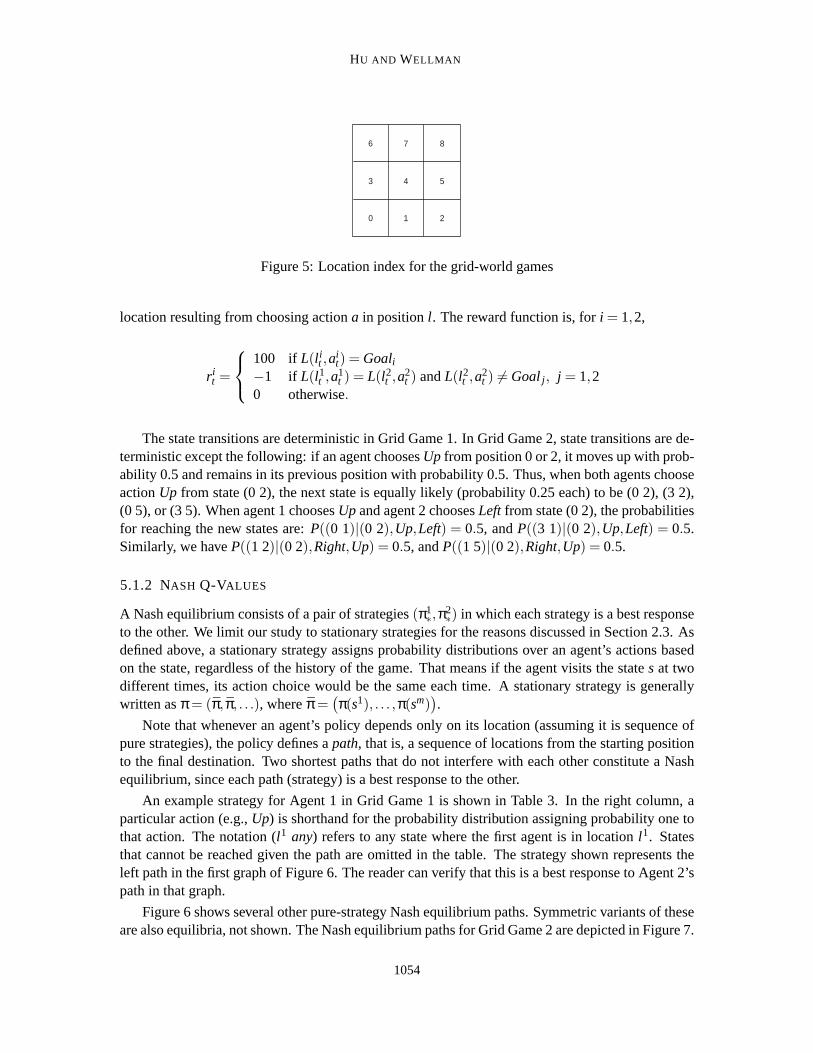
The action space of agenti, i = 1,2, is Ai ={Left, Right, Down, Up}. The state space isS={(0 1),(0 2), . . . ,(8 7)}, where a states = (l1, l2) represents the agents’ joint location. Agenti’slocationl i is represented by position index, as shown in Figure 5.5

If an agent reaches the goal position, it receives a reward of 100. If it reaches another positionwithout colliding with the other agent, its reward is zero. If it collides with the other agent, it receives−1 and both agents are bounced back to their previous positions. LetL(l ,a) be the potential new

4. Note that a payoff function is a correspondence from all state-action tuples to rewards. An agent may be able toobserve a particular reward, but still lack the knowledge of the overall payoff function.

5. Given that two agents cannot occupy the same position, and excluding the cases where at least one agent is in its goalcell, the number of possible joint positions is 57 for Grid Game 1 and 56 for Grid Game 2.

1053

HU AND WELLMAN

6 7 8

3 4 5

0 1 2

Figure 5: Location index for the grid-world games

location resulting from choosing actiona in positionl . The reward function is, fori = 1,2,

r it =

100 if L(l it ,a

it) = Goali

−1 if L(l1t ,a1

t ) = L(l2t ,a2

t ) andL(l2t ,a2

t ) 6= Goalj , j = 1,20 otherwise.

The state transitions are deterministic in Grid Game 1. In Grid Game 2, state transitions are de-terministic except the following: if an agent choosesUp from position 0 or 2, it moves up with prob-ability 0.5 and remains in its previous position with probability 0.5. Thus, when both agents chooseactionUp from state (0 2), the next state is equally likely (probability 0.25 each) to be (0 2), (3 2),(0 5), or (3 5). When agent 1 choosesUp and agent 2 choosesLeft from state (0 2), the probabilitiesfor reaching the new states are:P((0 1)|(0 2),Up,Left) = 0.5, andP((3 1)|(0 2),Up,Left) = 0.5.Similarly, we haveP((1 2)|(0 2),Right,Up) = 0.5, andP((1 5)|(0 2),Right,Up) = 0.5.

5.1.2 NASH Q-VALUES

A Nash equilibrium consists of a pair of strategies(π1∗,π2∗) in which each strategy is a best responseto the other. We limit our study to stationary strategies for the reasons discussed in Section 2.3. Asdefined above, a stationary strategy assigns probability distributions over an agent’s actions basedon the state, regardless of the history of the game. That means if the agent visits the states at twodifferent times, its action choice would be the same each time. A stationary strategy is generallywritten asπ = (π, π, . . .), whereπ =

(π(s1), . . . ,π(sm)

).

Note that whenever an agent’s policy depends only on its location (assuming it is sequence ofpure strategies), the policy defines apath, that is, a sequence of locations from the starting positionto the final destination. Two shortest paths that do not interfere with each other constitute a Nashequilibrium, since each path (strategy) is a best response to the other.

An example strategy for Agent 1 in Grid Game 1 is shown in Table 3. In the right column, aparticular action (e.g.,Up) is shorthand for the probability distribution assigning probability one tothat action. The notation (l1 any) refers to any state where the first agent is in locationl1. Statesthat cannot be reached given the path are omitted in the table. The strategy shown represents theleft path in the first graph of Figure 6. The reader can verify that this is a best response to Agent 2’spath in that graph.

Figure 6 shows several other pure-strategy Nash equilibrium paths. Symmetric variants of theseare also equilibria, not shown. The Nash equilibrium paths for Grid Game 2 are depicted in Figure 7.

1054

NASH Q-LEARNING

STATE s π1(s)(0 any) Up(3 any) Right(4 any) Right(5 any) Up

Table 3: A stationary strategy for agent 1 in Grid Game 1

Figure 6: Selected Nash equilibrium paths, Grid Game 1

The value of the game for agent 1 is defined as its accumulated reward when both agents followtheir Nash equilibrium strategies,

v1(s0) = ∑t

βtE(rt |π1∗,π

2∗,s0).

In Grid Game 1 and initial states0 = (0 2), this becomes, givenβ = 0.99,

v1(s0) = 0+0.99·0+0.992 ·0+0.993 ·100

= 97.0.

Based on the values for each state, we can then derive the Nash Q-values for agent 1 in states0,

Q1(s0,a1,a2) = r1(s0,a

1,a2)+β∑s′

p(s′|s0,a1,a2)v1(s′).

ThereforeQ1∗(s0,Right,Le f t)=−1+0.99v1((0 2))= 95.1, andQ1∗(s0,U p,U p)= 0+0.99v1((3 5))=97.0.

The Nash Q-values for both agents in state (0 2) of Grid Game 1 are shown in Table 4. Thereare three Nash equilibria for this stage game(Q1(s0),Q2(s0)), and each is a global optimal pointwith the value (97.0, 97.0).

For Grid Game 2, we can derive the optimal values similarly for agent 1:

v1((0 1)) = 0+0.99·0+0.992 ·0 = 0,

v1((0 x)) = 0, for x = 3, . . . ,8,

v1((1 2)) = 0+0.99·100= 99,

v1((1 3)) = 0+0.99·100= 99= v1((1 5)),v1((1 x)) = 0, for x = 4,6,8.

1055

HU AND WELLMAN

Figure 7: Nash equilibrium paths, Grid Game 2

Left UpRight 95.1, 95.1 97.0, 97.0

Up 97.0, 97.0 97.0, 97.0

Table 4: Grid Game 1: Nash Q-values in state (0 2)

However, the value forv1((0 2)) = v1(s0) can be calculated only in expectation, because the agentshave a 0.5 probability of staying in their current location if they chooseUp. We solvev1(s0) fromthe stage game(Q1∗(s0),Q2∗(s0)).

The Nash Q-values for agent 1 in states0 = (0 2) are

Q1∗(s0,Right,Left) = −1+0.99v1((s0)),

Q1∗(s0,Right,Up) = 0+0.99(

12

v1((1 2))+12

v1((1 3)) = 98,

Q1∗(s0,Up,Left) = 0+0.99(

12

v1((0 1))+12

v1((3 1)) = 0.99(0+12

99) = 49,

Q1∗(s0,Up,Up) = 0+0.99(

14

v1((0 2))+14

v1((0 5))+14

v1((3 2))+14

v1((3 5)))

= 0.99(14

v1((0 2))+0+14

99+14

99)

= 0.9914

v1(s0)+49.

These Q-values and those of agent 2 are shown in Table 5.1.2. We defineRi ≡ vi(s0) to be agenti’s optimal value by following Nash equilibrium strategies starting from states0, wheres0 = (0 2).

Given Table 5.1.2, there are two potential pure strategy Nash equilibria: (Up, Left) and (Right,Up). If (Up, Left) is the Nash equilibrium for stage game(Q1∗(s0),Q2∗(s0)), thenv1(s0)= π1(s0)π2(s0)Q1(s0)=49, and thenQ1∗(s0,Right,Left) = 47. Therefore we can derive all the Q-values as shown in thefirst table in Figure 8. If (Right, Up) is the Nash equilibrium,v1(s0) = 98, and we can deriveanother set of Nash Q-values as shown in the second table in Figure 8. In addition, there existsa mixed-strategy Nash equilibrium for stage game(Q1∗(s0),Q2∗(s0)), which is (π1(s0),π2(s0)) =({P(Right) = 0.97,P(Up) = 0.03)},{P(Left) = 0.97,P(Up) = 0.03}), and the Nash Q-values areshown in the third table of Figure 8.6

As we can see, there exist three sets of different Nash equilibrium Q-values for Grid Game 2.This is essentially different from Grid Game 1, which has a unique Nash Q-value for every state-

6. See Appendix A for a derivation.

1056

NASH Q-LEARNING

Left UpRight −1+0.99R1,−1+0.99R2 98, 49

Up 49, 98 49+ 140.99R1,49+ 1

40.99R2

Table 5: Grid Game 2: Nash Q-values in state (0 2)

Left UpRight 47, 96 98, 49

Up 49, 98 61, 73


Up 49, 98 73, 61

Left UpRight 47.87, 47.87 98, 49

Up 49, 98 61.2, 61.2

Figure 8: Three Nash Q-values for state (0 2) in Grid Game 2

action tuple. The convergence of learning becomes problematic when there are multiple Nash Q-values. Furthermore, none of the Nash equilibria of the stage game(Q1∗(s0),Q2∗(s0)) of Grid Game 2is a global optimal or saddle point, whereas in Grid Game 1 each Nash equilibrium is a globaloptimum.

5.1.3 THE LEARNING PROCESS

A learning agent, say agent 1, initializesQ1(s,a1,a2) = 0 andQ2(s,a1,a2) = 0 for all s,a1,a2. Notethat these are agent 1’s internal beliefs. They have nothing to do with agent 2’s beliefs. Here weare interested in how agent 1 learns the Nash Q-functions. Since learning is offline, it does notmatter whether agent 1 is wrong about agent 1’s actual strategies during the learning process. Butagent 1 has learned the equilibrium strategies, which stipulate what both agents will do when theyboth know enough information about the game and both act rationally.

A game starts from the initial state(0 2). After observing the current state, agents choosetheir actions simultaneously. They then observe the new state, both agents’ rewards, and the actiontaken by the other agent. The learning agent updates its Q-functions according to (8). In the newstate, agents repeat the process above. When at least one agent moves into its goal position, thegame restarts. In the new episode, each agent is randomly assigned a new position (except its goalcell). The learning agent keeps the Q-values learned from previous episodes. The training stopsafter 5000 episodes. Each episode on average takes about eight steps. So one experiment usuallyrequires about 40,000 steps. The total number of state-action tuples in Grid Game 1 is 424. Thuseach tuple is visited 95 times on average. The learning rate is defined as the inverse of the numberof visits. More specifically,αt(s,a1,a2) = 1

nt(s,a1,a2) , wherent(s,a1,a2) is the number of times

the tuple(s,a1,a2) has been visited. It is easy to show that this definition satisfies the conditionsin Assumption 2. Whenαt = 1

95 ≈ 0.01, the results from new visits hardly change the Q-valuesalready learned.

When updating the Q-values, the agent applies a Nash equilibrium value from the stage game(Q1(s′),Q2(s′)), possibly necessitating a choice among multiple Nash equilibria. In our implemen-

1057

HU AND WELLMAN

Left UpRight -1, -1 49, 0

Up 0, 0 0, 97

Table 6: Grid Game 1: Q-values in state (0 2) after 20 episodes if always choosing the first Nash


Up 0, 0 49, 49

Table 7: Grid Game 2: Q-values in state (0 2) after 61 episodes if always choosing the first Nash

tation, we calculate Nash equilibria using the Lemke-Howson method (Cottle et al., 1992), whichcan be employed to generate equilibria in a fixed order.7 We then define afirst-Nashlearning agentas one that updates its Q-values using the first Nash equilibrium generated. Asecond-Nashagentemploys the second if there are multiple equilibria, otherwise it uses the only available one. Abest-expected-Nashagent picks the Nash equilibrium that yields the highest expected payoff to itself.

5.2 Experimental Results

5.2.1 Q-FUNCTIONS DURING LEARNING

Examination of Q-values during learning reveals that both grid games violate Assumption 3. Table 6shows the results for first-Nash agents playing Grid Game 1 from state (0 2) after certain learningepisodes. The only Nash equilibrium in this stage game, (Right, Up), is neither a global optimumnor a saddle point. In Grid Game 2, we find a similar violation of Assumption 3. The unique Nashequilibrium (Up, Up) in the stage game shown in Table 7 is neither a global optimum nor a saddlepoint.

5.2.2 CONVERGENCERESULTS: THE FINAL Q-FUNCTIONS

After 5000 episodes of training, we find that agents’ Q-values stabilize at certain values. Somelearning results are reported in Table 8 and 9. Note that a learning agent always uses the same Nashequilibrium value to update its own Q-function and that of the other agent.

We can see that the results in Table 8 are close to the theoretical derivation in Table 4, and theresults in Table 9 are close to the theoretical derivation in the first table of Figure 8. Although it isimpossible to validate theoretical asymptotic convergence with a finite trial, our examples confirmthat the learned Q-functions possess the same equilibrium strategies asQ∗.

For each states, we derive a Nash equilibrium(π1(s),π2(s)) from the stage game comprising thelearned Q-functions,(Q1(s),Q2(s)). We then compare this solution to a Nash equilibrium derivedfrom theory. Results from our experiments are shown in Table 10. In Grid Game 1, our learningreaches a Nash equilibrium 100% of the time (out of 50 runs) regardless of the updating choiceduring learning. In Grid Game 2, however, learning does not always converge to a Nash equilibriumjoint strategy.

7. The Lemke-Howson algorithm is quite effective in practice (despite exponential worst-case behavior), but limited totwo-player (bimatrix) games.

1058

NASH Q-LEARNING


Up 96, 91 95, 95

Table 8: Final Q-values in state (0 2) if choosing the first Nash in Grid Game 1

Agent 1Left Up

Right 39, 84 97, 51Up 46, 93 59, 74

Table 9: Final Q-values in state (0 2) if choosing the first Nash in Grid Game 2

5.3 Offline Learning Performance

In offline learning, examples (training data) for improving the learned function are gathered in thetraining period, and performance is measured in the test period. In our experiments, we employ atraining period of 5000 episodes. The performance of the test period is measured by the reward anagent receives when both agents follow their learned strategies, starting from the initial positions atthe lower corners.

Since learning is internal to each agent, two agents might learn different sets of Q-functions,which yield different Nash equilibrium solutions. For example, agent 2 might learn a Nash equilib-rium corresponding to the joint path in the last graph of Figure 6. In that case, agent 2 will alwayschooseLeft in state (0 2). Agent 1 might learn the third graph of Figure 6, and therefore alwayschooseRight in state (0 2). In this case agent 1’s strategy is not a best response to agent 2’s strategy.

We implement four types of learning agents: first Nash, second Nash, best-expected Nash, andsingle–the single-agent Q-learning method specified in (4).

The experimental results for Grid Game 1 are shown in Table 11. For each case, we ran 50trials and calculated the fraction that reach an equilibrium joint path. As we can see from the table,when both agents employ single-agent Q-learning, they reach a Nash equilibrium only 20% of thetime. This is not surprising since the single-agent learner never models the other agent’s strategicattitudes. When one agent is a Nash agent and the other is a single-agent learner, the chance ofreaching a Nash equilibrium increases to 62%. When both agents are Nash agents, but use differentupdate selection rules, they end up with a Nash equilibrium 80% of the time.8 Finally, when bothagents are Nash learners and use the same updating rule, they end up with a Nash equilibriumsolution 100% of the time.

The experimental results for Grid Game 2 are shown in Table 12. As we can see from thetable, when both agents are single-agent learners, they reach a Nash equilibrium 50% of the time.When one agent is a Nash learner, the chance of reaching a Nash equilibrium increases to 51.3% onaverage. When both agents are Nash learners, but use different updating rules, they end up with aNash equilibrium 55% of the time on average. Finally, 79% of trials with two Nash learners usingthe same updating rule end up with a Nash equilibrium.

Note that during learning, agents choose their action randomly, based on a uniform distribution.Though the agent’s own policy during learning does not affect theoretical convergence in the limit

8. Note that when both agents employ best-expected Nash, they may choose different Nash equilibria. A Nash equilib-rium solution giving the best expected payoff to one agent may not lead to the best expected payoff for another agent.Thus, we classify trials with two best-expected Nash learners in the category of those using different update selectionrules.

1059

HU AND WELLMAN

Equilibrium selection Percentage of runs that reach aNash equilibrium

Grid Game 1 First Nash 100%Second Nash 100%

Grid Game 2 First Nash 68%Second Nash 90%

Table 10: Convergence Results

LEARNING STRATEGYRESULTS OF

LEARNING

AGENT 1 AGENT 2 PERCENT THAT

REACH A NASH

EQUILIBRIUM

SINGLE SINGLE 20%

SINGLEFIRST NASH 60%SECOND NASH 50%BEST EXPECTEDNASH 76%

FIRST NASH SECOND NASH 60%BEST EXPECTEDNASH 76%

SECOND NASH BEST EXPECTEDNASH 84%BEST EXPECTEDNASH BEST EXPECTEDNASH 100%FIRST NASH FIRST NASH 100%SECOND NASH SECOND NASH 100%

Table 11: Learning performance in Grid Game 1

(as long as every state and action are visited infinitely often), the policy of other agents does influ-ence the single-agent Q-learner, as its perceived environment includes the other agents implicitly.For methods that explicitly consider joint actions, such as NashQ, the joint policy affects only thepath to convergence.

For Grid Game 2, the single-single outcome can be explained by noting that given its counterpartis playing randomly, the agent has two optimal policies: entering the center and following thewall. To see their equivalence, note that if agent 1 choosesRight, it will successfully move withprobability 0.5 because agent 2 will chooseLeft with equal probability. If agent 1 choosesUp, itwill successfully move with probability 0.5 because this is the defined transition probability. Thevalue of achieving either location are the same, and therefore the two initial actions have the samevalue. Given that the agents learn that there are two equal-valued strategies, there is a 0.5 probabilitythat they will happen to choose the complementary ones, hence the result.

Alternative training regimens, in which agents’ policies are updated during learning, should beexpected to improve the single-agent Q-learning results. Indeed, both Bowling and Veloso (2002)and Greenwald and Hall (2003) found this to be the case in Grid Game 2 and other environments,

5.4 Online Learning Performance

In online learning, an agent is evaluated based on rewards accrued while it learns. Whereas ac-tion choices in the training periods of offline learning are important only with respect to gaining

1060

NASH Q-LEARNING

LEARNING STRATEGYRESULTS OF

LEARNING

AGENT 1 AGENT 2 PERCENT THAT

REACH A NASH

EQUILIBRIUM

SINGLE SINGLE 50%

SINGLEFIRST NASH 54%SECOND NASH 62%BEST EXPECTEDNASH 38%

FIRST NASH SECOND NASH 64%BEST EXPECTEDNASH 78%

SECOND NASH BEST EXPECTEDNASH 36%BEST EXPECTEDNASH BEST EXPECTEDNASH 42%FIRST NASH FIRST NASH 68%SECOND NASH SECOND NASH 90%

Table 12: Learning performance in Grid Game 2

information, in online learning the agent must weigh value for learning (exploration) against directperformance value (exploitation).

The Q-learning literature recounts many studies on the balance between exploration and ex-ploitation. In our investigation, we adopt anε-Greedy exploration strategy, as described, for exam-ple, by Singh et al. (2000). In this strategy, the agent explores with probabilityεt(s) and chooses theoptimal action with probability 1− εt(s). Singh et al. (2000) proved that whenεt(s) = c/nt(s) with0 < c < 1, the learning policy satisfies the GLIE (Greedy in the Limit with Infinite Exploration)property.

We test agent 1’s performance under three different strategies:exploit, explore, andexploit-and-explore. In the exploit strategy, an agent always chooses the Nash equilibrium learned so farif the state has been visited at least once (nt(s) ≥ 1). If nt(s) = 0, the agent will choose an actionrandomly. In the explore strategy, an agent chooses an action randomly. In the exploit-and-explorestrategy, the agent chooses the Nash equilibrium action with probabilityεt(s) = 1

1+nt(s)and chooses

a random action with probability 1− εt(s).Our results are shown in Figure 9. The experiments show that when the other agent plays

exploit, the exploit-and-explore strategy gives agent 1 higher payoff than the exploit strategy. Whenagent 2 is an explore or exploit-and-explore agent, agent 1’s payoff from exploit is very close to thatfrom exploit-and-explore, though the latter is still a little higher. One explanation for this is that theexploit strategy is very easily trapped in local optima. When one agent uses the exploit-and-explorestrategy, it helps that agent to find an action that is not in conflict with another agent, so that bothagents will benefit.

6. Related Work

Littman (1994) designed a Minimax-Q learning algorithm for zero-sum stochastic games. A con-vergence proof for that algorithm was provided subsequently by Littman and Szepesvari (1996).Claus and Boutilier (1998) implemented a joint action learner, incorporating other agents’ actionsinto its Q-function, for a repeated coordination game. That paper was first presented in a AAAI-97 workshop, and motivated our own work on incorporating joint actions into Q-functions in the

1061

HU AND WELLMAN

0 0.2 0.4 0.6 0.8 1 1.2 1.4 1.6 1.8 2

x 104

0

10

20

30

40

50

60

70

80

90

100Agent 2 is an Exploit agent

Steps in the game

Ave

rag

e r

ew

ard

of A

ge

nt 1

Agent 1:Explore AgentAgent 1: Exploit AgentAgent 1: Exploit−and−exploration agent

0 0.2 0.4 0.6 0.8 1 1.2 1.4 1.6 1.8 2

x 104

−20

0

20

40

60

80

100Agent 2 is an Exploit−and−exploration agent

Steps in the game

Ave

rag

e r

ew

ard

of A

ge

nt 1


0 0.2 0.4 0.6 0.8 1 1.2 1.4 1.6 1.8 2

x 104

−20

0

20

40

60

80

100Agent 2 is an Explore agent

Steps in the game

Ave

rag

e r

ew

ard

of A

ge

nt 1


Figure 9: Online performance of agent 1 in three different environments

general-sum context. Our Nash Q-learning algorithm (Hu and Wellman, 1998) was the subject offurther clarification from Bowling (2000) and illustrations from Littman (2001b).

The Friend-or-Foe Q-learning (FFQ) algorithm (Littman, 2001a) overcomes the need for our as-sumptions about stage games during learning in special cases where the stochastic game is known tobe a coordination game or zero-sum. In coordination games—where there is perfect correlation be-tween agents’ payoffs—an agent employs Friend-Q, which selects actions to maximize an agent’sown payoff. In zero-sum games—characterized by perfectnegativecorrelation between agents’payoffs—an agent uses Foe-Q, which is another name for Minimax-Q. In both cases, the correla-tions reduce the agents’ learning problem to that of learning its own Q-function. Littman shows thatFFQ converges generally, and to equilibrium solutions when the friend or foe attributions are cor-rect. His analysis of our two grid-world games (Section 5) further illuminates the relation betweenNashQ and FFQ.

1062

NASH Q-LEARNING

Sridharan and Tesauro (2000) have investigated the behavior of single-agent Q-learners in adynamic pricing game. Bowling and Veloso (2002) present a variant of single-agent Q-learning,where rather than adopt the policy implicit in the Q-table, the agent performs hill-climbing in thespace of probability distributions over actions. This enables the agent to maintain a mixed strategy,while learning a best response to the other agents. Empirical results (including an experiment withour Grid Game 2) suggest that the rate of policy hill climbing should depend on the estimated qualityof the current policy.

Researchers continue to refine Q-learning for zero-sum stochastic games. Recent developmentsinclude the work by Brafman and Tennenholtz (2000, 2001), who developed a polynomial-timealgorithm that attains near-optimal average reward in zero-sum stochastic games. Banerjee et al.(2001) designed a Minimax-SARSA algorithm for zero-sum stochastic games, and presented evi-dence of faster convergence than Minimax-Q.

One of the drawbacks of Q-learning is that each state-action tuple has to be visited infinitelyoften. Q(λ) learning (Peng and Williams, 1996, Wiering and Schmidhuber, 1998) promises an inter-esting way to speed up the learning process. To apply Q-learning online, we seek a general criterionfor setting the exploitation rate, which would maximize the agent’s expected payoff. Meuleau andBourgine (1999) studied such a criterion in single-agent multi-state environments. Chalkiadakisand Boutilier (2003) proposed using Bayesian beliefs about other agents’s strategies to guide thecalculation. Since fully Bayesian updating is computationally demanding, in practice they updatestrategies based on fictitious play.

This entire line of work has raised questions about the fundamental goals of research in multia-gent reinforcement learning. Shoham et al. (2003) take issue with the focus on convergence towardequilibrium, and propose four alternative, well-defined problems that multiagent learning mightplausibly address.

7. Conclusions

We have presented NashQ, a multiagent Q-learning method in the framework of general-sum stochas-tic games. NashQ generalizes single-agent Q-learning to multiagent environments by updating itsQ-function based on the presumption that agents choose Nash-equilibrium actions. Given somehighly restrictive assumptions on the form of stage games during learning, the method is guaran-teed to converge. Empirical evaluation on a pair of small but interesting grid games shows that themethod can often find equilibria despite the violations of our theoretical assumptions. In particular,in a game possessing multiple equilibria with identical values, the method converges to equilibriumwith relatively high frequency. In a second game with a variety of equilibrium Q-values, the ob-served likelihood of reaching an equilibrium is reduced. In both cases, however, employing NashQimproves the prospect for reaching equilibrium over single-agent Q-learning, at least in the offlinelearning mode.

Although NashQ is defined for the general-sum case, the conditions for guaranteed convergenceto equilibrium do not cover a correspondingly general class of environments. As Littman (2001a,b)has observed, the technical conditions are actually limited to cases—coordination and adversarialequilibria—for which simpler methods are sufficient. Moreover, the formal condition (Assump-tion 3) underlying the convergence theorem is defined in terms of the stage gamesas perceivedduring learning, so cannot be evaluated in terms of the actual game being learned. Of what value,

1063

HU AND WELLMAN

then, are the more generally cast algorithm and result? We believe there are two main contributionsof the analysis presented herein.

First, it provides a starting point for further theoretical work on multiagent Q-learning. Certainlythere is much middle ground between the extreme points of pure coordination and pure zero-sum,and much of this ground will also be usefully cast as special cases of Nash equilibrium.9 The NashQanalysis thereby provides a known sufficient condition for convergence, which may be relaxed inparticular circumstances by taking advantage of other known structure in the game or equilibrium-selection procedure.

Second, at present there isno multiagent learning method offering directly applicable perfor-mance guarantees for general-sum stochastic games. NashQ is based on intuitive generalization ofboth the single-agent and minimax methods, and remains a plausible candidate for the large bodyof environments for which no known method is guaranteed to work well. One might expect itto perform best in games with unique or concentrated equilibria, though further study is requiredto support strong conclusions about its relative merits for particular classes of multiagent learningproblems.

Perhaps more promising than NashQ itself are the many conceivable extensions and variantsthat have already begun to appear in the literature. For example, the “extended optimal response”approach (Suematsu and Hayashi, 2002) maintains Q-tables for all agents, and anticipates the otheragents’ actions based on a balance of their presumed optimal and observed behaviors. Anotherinteresting direction is reflected in the work of Greenwald and Hall (2003), who propose a versionof multiagent Q-learning that employscorrelated equilibriumin place of the Nash operator appliedby NashQ. This appears to offer certain computational and convergence advantages, while requiringsome collaboration in the learning process itself.

Other equilibrium concepts—such as any of the many Nash “refinements” defined by gametheorists—specify by immediate analogy a variety of multiagent Q-learning. It is our hope that anunderstanding of NashQ can assist search through all the plausible variants and hybrids, toward theultimate goal of designing effective learning algorithms for dynamic multiagent domains.

Appendix A. A Mixed Strategy Nash Equilibrium for Grid Game 2

We are interested in determining if there exists a mixed strategy Nash equilibrium for Grid Game2. LetRi ≡ vi(s0) be agenti’s optimal value by following Nash equilibrium strategies starting fromstates0, wheres0 = (0 2). The two agents’ Nash Q-values for taking different joint actions in states0 are shown in Table 5.1.2. The Nash Q-value is defined as the sum of discounted rewards oftaking a joint action at current state (in states0) and then following the Nash equilibrium strategiesthereafter.

Let (p,1− p) be agent 1’s probabilities of taking actionRightandUp, and(q,1−q) be agent 2’sprobabilities of taking actionLeftandUp. Then agent 1’s problem is

maxp

p[q(−1+0.99R1)+(1−q)98]+ (1− p)[49q+(1−q)(49+ 140.99R1]

s.t. p≥ 0

9. Indeed, the classes of games thatpossess, respectively, coordination or adversarial equilibria, are already far relaxedfrom the pure coordination and zero-sum games, which were the focus of original studies establishing behaviors ofthe equivalents of Friend-Q and Foe-Q.

1064

NASH Q-LEARNING

Left UpRight 47.87, 47.87 98, 49

Up 49, 98 61.2, 61.2

Table 13: Nash Q-values in state (0 2)

Let µ be the Kuhn-Tucker multiplier on the constraint, so that the Lagrangian takes the form:

L = p[0.99R1q+98−99q]+ (1− p)[49+0.2475R1−0.2475R1q]−µp

The maximization condition requires that∂L∂p

= 0. Therefore we get

0.99R1q+98−99q−49−0.2475R1 +0.2475R1q = µ. (18)

Since we are interested in mixed strategy solution wherep> 0, the slackness condition implies thatµ= 0. Based on equation (18), we get

R1 =99q−49

1.2375q−0.2475. (19)

By symmetry in agent 1 and 2’s payoffs, we also have

R2 =99p−49

1.2375p−0.2475.

By definition,R1 = v1(s0). According to Lemma 10,v1(s0) = π1(s0)π2(s0)Q1(s0). Sinceπ1(s0) =(p 1− p) andπ2(s0) = (q 1−q), therefore

R1 = (p 1− p)( −1+0.99R1 98

49 49+ 140.99R1

)(q

1−q

)

= pq(−1+0.99R1)+(1−q)p98+49q(1− p)+(1−q)(1− p)(49+0.2475R1).

From the above equation and (19), we have

−24.745+1.7325q+24.5025q2 = 0,

and solving yieldsq = 0.97.By symmetry in the two agents’ payoff matrices, we havep = 0.97.Therefore we haveR1 = R2 = 99×0.97−49

1.2375×0.97−0.2475 = 49.36. We can then rewrite Table 5.1.2 asTable 13.

Acknowledgments

We thank Craig Boutilier, Michael Littman, Csaba Szepesvari, Jerzy Filar, and Olvi Mangasarianfor helpful discussions. The anonymous referees provided invaluable criticism and suggestions.

1065

HU AND WELLMAN

References

Tucker Balch. Learning roles: Behavioral diversity in robot teams. In Sandip Sen, editor,CollectedPapers from the AAAI-97 Workshop on Multiagent Learning. AAAI Press, 1997.

Cesar Bandera, Francisco J. Vico, Jose M. Bravo, Mance E. Harmon, and Leemon C. Baird. Resid-ual Q-learning applied to visual attention. InThirteenth International Conference on MachineLearning, pages 20–27, Bari, Italy, 1996.

Bikramjit Banerjee, Sandip Sen, and Jing Peng. Fast concurrent reinforcement learners. InSeven-teenth International Joint Conference on Artificial Intelligence, pages 825–830, Seattle, 2001.

Craig Boutilier. Sequential optimality and coordination in multiagent systems. InSixteenth Inter-national Joint Conference on Artificial Intelligence, pages 478–485, Stockholm, 1999.

Michael Bowling. Convergence problems of general-sum multiagent reinforcement learning. InSeventeenth International Conference on Machine Learning, pages 89–94, Stanford, 2000.

Michael Bowling and Manuela Veloso. Multiagent learning using a variable learning rate.ArtificialIntelligence, 136:215–250, 2002.

Ronen I. Brafman and Moshe Tennenholtz. A near-optimal polynomial time algorithm for learningin certain classes of stochastic games.Artificial Intelligence, 121(1-2):31–47, 2000.

Ronen I. Brafman and Moshe Tennenholtz. A general polynomial time algorithm for near-optimalreinforcement learning. InSeventeenth International Joint Conference on Artificial Intelligence,pages 953–958, Seattle, 2001.

Georgios Chalkiadakis and Craig Boutilier. Coordination in multiagent reinforcement learning: abayesian approach. InThe Proceedings of the Second International Conference on AutonomousAgents and Multiagent Systems (AAMAS 2003), pages 709–716, 2003.

Caroline Claus and Craig Boutilier. The dynamics of reinforcement learning in cooperative mul-tiagent systems. InFifteenth National Conference on Artificial Intelligence, pages 746–752,Madison, WI, 1998.

Richard W. Cottle, J.-S. Pang, and R. E. Stone.The Linear Complementarity Problem. AcademicPress, New York, 1992.

Edwin De Jong. Non-random exploration bonuses for online reinforcement learning. In SandipSen, editor,Collected Papers from the AAAI-97 Workshop on Multiagent Learning. AAAI Press,1997.

Jerzy Filar and Koos Vrieze.Competitive Markov Decision Processes. Springer-Verlag, 1997.

A. M. Fink. Equilibrium in a stochasticn-person game.Journal of Science in Hiroshima University,Series A-I, 28:89–93, 1964.

Drew Fudenberg and David K. Levine.The Theory of Learning in Games. The MIT Press, 1998.

1066

NASH Q-LEARNING

Amy Greenwald and Keith Hall. Correlated Q-learning. InProceedings of the Twentieth Interna-tional Conference on Machine Learning (ICML-2003), pages 242–249, Washington DC, 2003.

Stephan H. G. ten Hagen. Continuous State Space Q-Learning for Control ofNonlinear Systems. PhD thesis, University of Amsterdam, February 2001.http://carol.wins.uva.nl/˜stephanh/phdthesis/.

John C. Harsanyi and Reinhard Selten.A General Theory of Equilibrium Selection in Games. TheMIT Press, 1988.

Junling Hu. Learning in Dynamic Noncooperative Multiagent Systems. PhD thesis, University ofMichigan, Ann Arbor, Michigan, July 1999.

Junling Hu and Michael P. Wellman. Multiagent reinforcement learning: Theoretical frameworkand an algorithm. InFifteenth International Conference on Machine Learning, pages 242–250,Madison, WI, 1998.

Junling Hu and Michael P. Wellman. Experimental results on Q-learning for general-sum stochasticgames. InSeventeenth International Conference on Machine Learning, pages 407–414, Stanford,2000.

Rufus Isaacs.Differential Games: A Mathematical Theory with Applications to Warfare and Pur-suit, Control and Optimization. R. E. Krieger Pub. Co., 1975.

Leslie Kaelbling, Michael L. Littman, and Andrew W. Moore. Reinforcement learning: A survey.Journal of Artificial Intelligence Research, 4:237–285, 1996.

Michael Kearns, Michael L. Littman, and Satinder Singh. Graphical models for game theory. InSeventeenth Conference on Uncertainty in Artificial Intelligence, pages 253–260, Seattle, 2001.

Jeffrey O. Kephart and Gerald J. Tesauro. Pseudo-convergent Q-learning by competitive pricebots.In Seventeenth International Conference on Machine Learning, pages 463–470, Stanford, 2000.

Daphne Koller and B. Milch. Multi-agent influence diagrams for representing and solving games. InSeventeenth International Joint Conference on Artificial Intelligence, pages 1027–1034, Seattle,Washington, 2001.

Michael L. Littman. Markov games as a framework for multi-agent reinforcement learning. InEleventh International Conference on Machine Learning, pages 157–163. New Brunswick, 1994.

Michael L. Littman. Friend-or-foe Q-learning in general-sum games. InEighteenth InternationalConference on Machine Learning, pages 322–328, Williams College, MA, 2001a.

Michael L. Littman. Value-function reinforcement learning in Markov games.Cognitive SystemsResearch, 2:55–66, 2001b.

Michael L. Littman and Csaba Szepesvari. A generalized reinforcement-learning model: Conver-gence and applications. InThirteenth International Conference on Machine Learning, pages310–318, 1996.

1067

HU AND WELLMAN

Richard D. McKelvey and Andrew McLennan. Computation of equilibria in finite games. InHand-book of Computational Economics, volume 1. Elsevier, 1996.

Nicolas Meuleau and Paul Bourgine. Exploration of multi-state environments: Local measures andback-propagation of uncertainty.Machine Learning, 35(2):117–154, 1999.

Tom Mitchell. Machine Learning, pages 367–390. McGraw-Hill, 1997.

John F. Nash. Non-cooperative games.Annals of Mathematics, 54:286–295, 1951.

Norihiko Ono and Kenji Fukumoto. Mulit-agent reinforcement learning: A modular approach. InSecond International Conference on Multiagent Systems, pages 252–258, Kyoto, 1996.

Martin J. Osborne and Ariel Rubinstein.A Course in Game Theory. MIT Press, 1994.

Jing Peng and Ronald Williams. Incremental multi-step Q-learning.Machine Learning, 22:283–290, 1996.

Leon A. Petrosjan and Nikolay A. Zenkevich.Game Theory. World Scientific, Singapore, 1996.

Martin L. Puterman.Markov Decision Processes: Discrete Stochastic Dynamic Programming. JohnWiley & Sons, New York, 1994.

Yoav Shoham, Rob Powers, and Trond Grenager. Multi-agent reinforcement learning: A criticalsurvey. Technical report, Stanford University, 2003.

Satinder Singh and Dimitri Bertsekas. Reinforcement learning for dynamic channel allocation incellular telephone systems. InAdvances in Neural Information Processing Systems, volume 9,pages 974–980. MIT Press, 1996.

Satinder Singh, Tommi Jaakkola, Michael L. Littman, and Csaba Szepesvari. Convergence resultsfor single-step on-policy reinforcement learning algorithms.Machine Learning, 38(3):287–308,2000.

Manu Sridharan and Gerald Tesauro. Multi-agent Q-learning and regression trees for automatedpricing decisions. InSeventeenth International Conference on Machine Learning, pages 927–934, Stanford, 2000.

Peter Stone and Richard S. Sutton. Scaling reinforcement learning toward RoboCup soccer. InProc. 18th International Conf. on Machine Learning, pages 537–544. Morgan Kaufmann, SanFrancisco, CA, 2001.

Nobuo Suematsu and Akira Hayashi. A multiagent reinforcement learning algorithm using extendedoptimal response. InFirst International Joint Conference on Autonomous Agents and MultiagentSystems, pages 370–377, Bologna, 2002.

Richard S. Sutton and Andrew G. Barto.Reinforcement Learning: An Introduction. MIT Press,1998.

Csaba Szepesvari and Michael L. Littman. A unified analysis of value-function-basedreinforcement-learning algorithms.Neural Computation, 11:8:2017–2059, 1999.

1068

NASH Q-LEARNING

Ming Tan. Multi-agent reinforcement learning: Independent vs. cooperative agents. InTenth Inter-national Conference on Machine Learning, pages 330–337, Amherst, MA, 1993.

Frank Thusijsman.Optimality and Equilibria in Stochastic Games. Centrum voor Wiskunde enInformatica, Amsterdam, 1992.

Marilyn A. Walker. An application of reinforcement learning to dialogue strategy selection in aspoken dialogue system for email.Journal of Artificial Intelligence Research, 12:387–416, 2000.

Christopher J. C. H. Watkins.Learning from Delayed Rewards. PhD thesis, King’s College, Cam-bridge, England, 1989.

Christopher J. C. H. Watkins and Peter Dayan. Q-learning.Machine Learning, 3:279–292, 1992.

Michael P. Wellman and Junling Hu. Conjectural equilibrium in multiagent learning.MachineLearning, 33:179–200, 1998.

Marco Wiering and Jurgen Schmidhuber. Fast online Q(λ). Machine Learning, 33:105–115, 1998.

1069

nash q-learning for general-sum stochastic...

Documents