. , ,

-!

( '.

~

NASA Contractor Report 172124

VISCOELASTIC STUDY OF AN ADHESIVELY BONDED JOINT

Paul F. Joseph

LEHIGH UNIVERSITY Bethlehem, Pennsylvania 18015

Grant NGR 39-007-011 April 1983

Nl\SI\ National Aeronautics and Space Administration

Langley Research Center Hampton. Virginia 23665

NASA-CR-172124 19830015359

liBRARY COpy .;UN 1 71983

LANGL2f RESEARCH CENTER Ll8RARY. NASA

HAMPTON,. VIRG!NIA

1111111111111 1111 111111111111111 I111I 11111111 NF01852

https://ntrs.nasa.gov/search.jsp?R=19830015359 2020-04-27T14:09:19+00:00Z

Abstract

In this study the plane strain problem of two dissimilar

orthotropic plates bonded with an isotropic, linearly viscoelastic

adhesive is considered. Both the shear and the normal stresses

in the adhesive are calculated for various geometries and loading

conditions. Transverse shear deformations of the adherends are

taken into account, and their effect on the solution is shown in

the results. All three in-plane strains of the adhesive are

included. Attention is given to the effect of temperature, both

in the adhesive joint problem in Part I and in a separate study

of heat generation in a viscoelastic material under cyclic loading

presented in Part II. This separate study is included because

heat generation and or spacially varying temperature are at pres­

ent too difficult to account for in the analytical solution of

the bonded joint, but whose effect can not be ignored in design.

In Part I if the temperature is taken as a known piecewise

constant function of time, the differential equations have constant

coefficients and the Laplace Transform technique can be directly

applied. In the heat generation problem the one-dimensional coupled

heat equation is solved. It is shown ,that the coupling term is

negligible. Both experimental and theoretical results are given

for various cycling frequencies.

-1-

An extension of the joint problem in Part I is a calculation

from fracture mechanics of the strain energy release rate when

debonding of the jOint takes place. The fracture energy is found

to be nearly independent of the bond length for lengths consistent

with a plate theory.

-2-

Part I

The Adhesive Joint

1. Introduction

Bonding as a means of attachment and as a way for reinforce­

ment is currently in wide use in the aerospace industry. Its main

mechanical advantage over riveting is that the load is carried

over a larger area, thus reducing the stress concentration.

Another advantage is that no holes are required which favors the

use of high strength, low weight fiber reinforced composites.

Indeed the development of these materials is achieved through a

bonding process.

However, bonding of joints has its own problems. Unfortunately

the load is not carried over the entire bond area, but instead is

confined to a small region along the bond edge. This highly

stressed region, though not as high as the stresses at a rivet,

can lead to one of several modes of failure. First consider the

failure of the adherends (for geometry of the joint see figures 1a,b).

At the edge of the bond region there are very high stresses in

both the adherends and the adhesive. In linear elasticity these

stresses are actually singular (see [1],[2]). However, because

of the geometrical complexities involved in an adhesive joint -

the combining of three distinct materials - several simplifications

-3-

of the three-dimensional elasticity problem are made. The adhe­

sive is modeled as a tension, shear spring by averaging all

stresses and strains through the thickness and the adherends are

modeled as plates. Therefore these singular stresses are not

observed, and it can be shown that all stresses are bounded. It

is of interest to note that even if the thickness variation of

stresses in the adhesive is ignored, the. normal stress in the x­

direction in the adherend will have a logarithmic singularity at

the bond edge. This results from the discontinuous shear trac­

tion acting on the surface of the adherend. The normal stress in

the adhesive does not cause any singular stresses in the adherends

(see [3]). Due to these high stresses, the adherends could fail

either by yielding of the material or by some form of material

separation such as cracking in the case of isotropic adherends, or

delamination in the case of laminated adherends. Cracking would

probably be attributed to the shear stress; delamination or trans­

verse pulling apart of the fiber layers is most likely the result

of the normal stress. Yielding could be attributed to both

stresses.

In order to analyze the failure of the adherends, one should

treat them as elastic continua. In this and most other studies,

the adherends are modeled as plates, and therefore the high

singular stress region in the adherend at the edge of the bond

-4-

is not observed. There are sev~ral papers that treat either one

or both of the adherends as elastic continua [4-6]. However, in

[6] it is found that there are severe convergence problems when

the adherends are relatively thin and this is precisely the geo­

metry when adherend failure becomes dominant as pointed out in

[7]. It is possible to analyse failure of the adherends if the

bending stresses due to eccentricity of the load path are taken

into account as was first investigated in [8] (see figures 2a,b).

This involves determination of the loading condition in figure 2b

in terms of the loading and geometry of figure 2a. Equilibrium

must actually be considered in the loaded position and therefore

this is a nonlinear procedure. In this study the loads of figure

2b are assumed known.

If the adherends are thick enough sothat adherend failure is

unlikely, cracking or peeling of the adhesive may result due to

high shear and normal stresses at the bond edge. This is a mixed

mode fracture mechanics problem where the shear stress can be more

important than the normal stress. In this study the strain energy

release rate is calculated, which may be used as the measure of

the magnitude of the external loads and the severity of joint geo­

metry in fatigue and fracture analysis.

r~st of the effort in the literature has been devoted to the

calculation of the adhesive stresses. It is in t.he constitutive

-5-

modeling of the adhesive that the various investigations differ.

They vary from elastic to a nonlinear viscoelastic behavior [2].

It is true that the epoxy which is subjected to such high stresses

at the bond edge will not behave in a linear way. An elastic­

plastic modeling of the adhesive is perhaps the simplest way to

incorporate this nonlinearity of material behavior.j However, the

analytical solution of such a formulation is very complicated (see

for example [1]). A viscoplastic solution, which incorporates all

other mentioned theories, is better still but an accurate analysis

requires a purely numerical technique such as finite elements.

The analytical solution presented in this study uses a linear

viscoelastic modeling of the adhesive. The hereditary integral

formulation is used and therefore the model is an accurate one. It

requires the relaxation modulus in shear which can be any function,

and, for practical applications, can be obtained from a fit to the

experimental data. The second material "constant" needed to define

an isotropic material is the bulk modulus which is assumed to be

time independent. This means that under a hydrostatic state of

stress the material behaves elastically. It is an assumption which

is quite commonly made. A check of this assumption was performed

using experimental data for an epoxy resin, Hercules 3S0l-SA.

This data was obtained from [9]. They fit curves to data for both

the relaxation modulus in shear (G(t» and in tension (E(t». To

obtain the bulk modulus (K(t», a Laplace Transform involving E(t)

and G(t) must be inverted. One can simplify the analysis by

-6-

assuming K to be constant and then hopefully having this verified.

For the given material, K proved to be nearly constant when com­

pared to E and G.

As far as the plate modeling is concerned, it is generally

accepted that transverse shear deformations should be taken into

account because of the high stresses involved. In this study this

addition involved very little extra algebra because the problem

was solved under the plane strain assumption. Also the order of

the differential equations for the stresses was not increased.

The inclusion of any extra degree of freedom for the plate beyond

what is provided by the Classical theory will probably have some

affect on the stresses. A more advanced plate theory was used

in [10] where the strain in the normal direction to the plate

\'ias non-zero. At the bond edge one can imagine a pinching effect

to exist making this quantity nonnegligible. Apparently this addi­

tion changes the order of the differential equation and there is a

requirement for an "extra II boundary condition. The researchers

of [10] forced the shear stress to be zero at the bond edge (i.e.,

T=O at x=±!I.). Since the stresses in the adhesive layer are aver­

aged through the thickness, one can not specify an elasticity

boundary condition and ignore the corners of the adhesive where

the stresses are singular. Perhaps another boundary condition could

be employed (see [1]).

-7-

The problem considered in this investigation 'is a further

generalization of work done by F. Delale and F. Erdogan [1,11,12].

It was in [1)] \-/hen they presented the viscoelastic solution for

identical adherends. In [1] they were joined by M.N. Ayduroglu

to publish a paper on the general elastic closed-form solution

with a finite element check of their results. It was shown in

this report that within geometrical restrictions the plate theory

gives good results for the normal and shear stress in the adhesive.

The restrictions are roughly that the ratio of adherend thickness

to adhesive thickness should be approximately an order of magnitude

and the ratio of bond length to adherend thickness should also be

an order of magnitude. Then in [12] further research by Delale

and Erdogan incl uded the infl uence of temperature on the adhesive

and how it affects the stresses. Here the adherends were identi­

cal and therefore no thermal stresses were present. In this study

the problem with dissimilar orthotropic adherends is considered.

This change, besides including thermal stresses, makes the solution

useful.

2. Fonnulation of the Problem

The problem considered is either the single lap joint (figure

la) or the cover plate (figu~e lb). A plate theory is used taking

into account transverse shear deformations. Also the problem will

-8-

be solved under the plane strain or cylindrical bending assumption

which requires that the geometry and loading are constant in the

z-direction.- The only independent spacial variable is x. The

viscoelastic nature of the adherend also makestime "tll an indepen­

dent variable.

Equilibrium of the element shown in figure 3a gives the fol­

lowing relationships:

aN lx --= T ax

aQ --.!.! = a ax

(ia ,b)

aQ2x --= -a

ax (2a,b)

(3a,b)

Nix' Qix' and Nix (i=1,2) are respectively the resultant

normal force, resultant shear force, and resultant bending moment

in the adherends. The adhesive stresses are T~ the shear stress,

and a, the transverse normal stress also shown in figure 3a.

Taking (T-To)H(t-t2) as the temperature function where T-To

is a constant and H(t) is the unit step function, the stress

resultant-displacement relations for the adherends are:

(4a,b)

-9-

as,-_1 = DiM. ax 1X

i = 1,2 , (Sa,b)

i = 1,2 , (6a,b)

where

(7)

and u and v are the x and y components of displacement of the mid­

plane of the adherends and S is the rotation of the normal. Note

that the term Qix/Bi includes the effect of transverse shear.

Since the adhesive is thin compar,ed to the adherends, the

average values of the strains are used - i.e. the y variation is

neglected. See figure lc for these kinematical considerations.

"y = (vl-v2) /ho

.. = x aUl hl aSl x aU2 h2 aS2x (-ax - Tax + ax + T--ax)/2 (Ba,b,c)

The hereditary integral approach will be used to model the

adhesive. For a linear, isotropic,viscoelastic adhesive we can

write:

t ae .. Sij = 2 f G(T,t-~)' a~J d~ (i ,j=x,y,z) t (9)

-co

-10-

(l0)

where

and

In the adhesive the only non-zero stresses are axx ' Txy = T,

ayy = a, and az and the only non-zero strains are EX' Ey' and yxY'

Substitution of (11) and (12) into (9) and (10) taking into

account the preceeding, we get:

_CIO

_CIO

t 3E 3€ 2az-ax-a = -2 J G(T,t-~)(~ + ~)d~

3~ a~ _CIO

t ay T = f G(T, t-~) ..2Y... d~

3~ _CIO

-11-

( 13)

(14)

(15)

( 16)

Since ESii = a and Eeii = 0, equations (13-15) are linearly

dependent; (14), for example, can be obtained by adding (13) and

(15), so it is ignored. Eliminating Ox and Oz from (13), (15),

and (17), it follows that

( 18)

Equations (1-6), (16) and (18) now make it possible to solve

3. The General Solution

We are interested mainly in ° and T so the other variables

are eliminated through algebra as follows.

Differentiate equations (5a,b) three times with respect to

x and make use of relations (3) and (2) to obtain

a3s h +h lx = D (<1 _ lOll) -a-x ..... 3;.;. 1 2 ax (19a)

( 19b)

Next take equation (16) and substitute for Yxy.

1 ft a h1 h2 T = ho G(T, t-~) 3i" (u1 -"'2 slx - u2 - "'2 s2x)d~ • (20)

-co

-12 ...

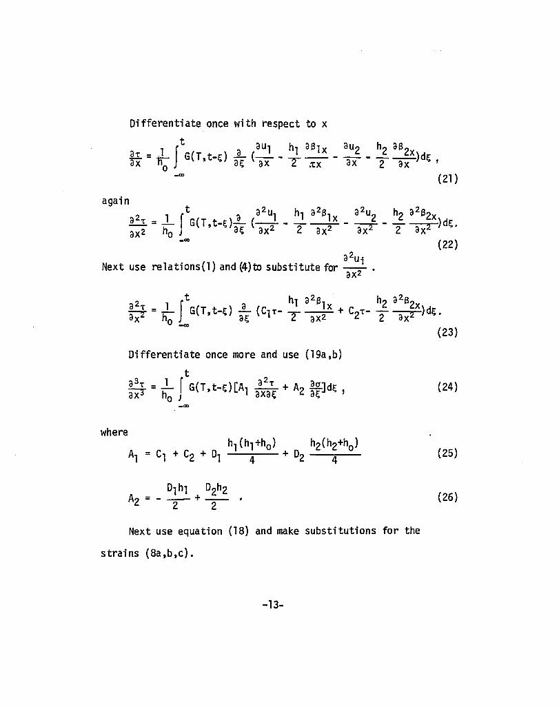
Differentiate once with respect to x

t a _ 1 J a aUl hl aSl x aU2 h2 as2x ~ - ir G(T,t-d - (- - ~- - - - ---)d~ ax 0 a!; ax £. .. tX ax 2 ax 1

_m (21)

a2u· Next use relations(l) and (4)to substitute for --' • ax2

where

Differentiate once more and use (19a,b)

t a3

• = _1 r G(T t-!;) [A a2• + A aO]d!;

~ ho J ' 1 axa!; 2 a~ ,

Next use equation (18) and make substitutions for the

strains (8a,b,c).

-13-

(22)

(24)

(25)

(26)

- h2 (v1-v2}]d~ • o

(27)

Differentiate once with respect to x and substitute using

(6) and (4) together with (1)

aa 1 Q1 x Q2x ' 1 ax = K(T}[ho

(B'1- B1x - 82 + B2x) + 2" (Crr - C2T

_CD

2 Q1x Q2x - - (- - 131 - - + 132 }]d~ • ho 81 x 82 x

(28)

Differentiate again using (2), (19)

-14-

2 '1 a 61 1 a 6 a a = K(T)[l (61 a - __ x + a + ~) axz- ho 1 ax B2 ax

1 . . hl hl+ho h2 h2+ho + tc(Cl-C2) ~~ - 01 T (0- 2 ~)-D2 T (0+ 2 ~~)]]

- ~ JtG(T,t-~) J... [ltc1

!!.. - C2 !!.. - 01 ~ (a- hl+ho !!..) 3 a~ '2\ ax ax 2 2 ax

_110

Differentiate once more

_110

(30)

Differentiate again making use of (19)

-15-

_00 (31)

where

(32)

(33)

(34)

(35)

(36)

Now assume that the temperature level is suddenly fixed at

0- with joint stress free. Now take Laplace Transform of equations

(24), and (31)

(37)

-16-

Now solving (37) for a

(39)

where

(40)

Rearranging (38)

(41)

substituting (39) into (41) we obtain

(42)

where

(43)

and

-17 ..

· -01 h1 ° h2 a = 1 G{T s) [ + -L- ] 2 n-' 2 2 o

2 °lh1 °2h2 2 2 + 3" ~(T'S)S[.--r- + -4- + hoB1 + hoB2 ]

4 01 02 a4 = [K{T) + 3 s G{T,s)][- ~ - ~ ]

o 0

(44)

Since the coefficients in equation (42) are not x dependent,

we look for a solution of the fonm emx•

The characteristic equation becomes

m7 + c1 ms + c2u3 + c3m = 0 •

-18-

(45)

Say this equation has the roots

0, ±Y1' ±Y2' ±Y3 (46)

\.,here Y1' Yi and Y3 are the roots of

y3 + c1y2 + c2Y + c3 = 0 . (47)

The solution is then

T(x,s) = Ao+A1sinhY1x+A2coshY1x+A3sinhY2x + A4coshY2x

+ A5sinhY3x + A6coshY3x

which may be written as

(48)

3 T(x,s) = Ao + i=l (A2i -1 sinhyix + A2i coshYix). (49)

From (gel) we find

~he constants Ai (i=0, ••• ,6) are detennined from the boundary

conditions. The seven relations to be used to obtain these con-

stants are the second and third derivatives of equation (18)

(equations 29 and 30), the first and second derivatives of equation

(16) (equations 21 and 22), and the following three relations which

refer to figure 3b. 1

f T(x,t)dx = N2(-t)H(t-t1)-No H(t-t1) -t

-19-

(51)

9. f a(x,t}dx = Q2(-~)H(t-tl)-QoH(t-tl) J -9.

f9. ho +h2

J xa(x,t)dx = [Mo-M2(-9.)+N2(-9.) 2 - 9.Qo - 1Q2(-1) _1

(52)

(53)

Now the laplace Transform of these seven expressions must

be taken. They become

2 Dlhl D2h2 - - s G(T,s)(- - - ......,..- - _2_ - -L

3 4 ~ hoBl hoB2

a- 2 - Dlhl D2h2 1 + a~ [(K(T)- 3" ~ G(T,S})(T'hl+ho)- -=a=<h2+ho»+ t< Cl+c2»1

D ~ D ~ _. 0 ~ 0 ~ + [K(T)(- 1 lx + 2 2x)+ 4 G(T,s)s(- 1 lx + 22X)],

ho ho 3 ho ho (54)

and

-20-

3 - _. 1 01 h1 D2h2 o cr = ocr [K(T)(- + 1 ____ )_ 2 s G(T ,s) a?" ax hoBl hoB2 4 4 J

Dlhl D2h2 2 x(- _- _____ 2_)] 4 4 hoBl hoB2

a2T 2 - Dlhl °2h2 1 + 3X2 [(K(T)- 3 SG(T,S))(~ (hl+ho)- -8- (h2+ho))+ 2(Cl-C2))]

°1 + [K(T)(- -ho

2 - h101 h1+h a T _ Gs [C - (Q- 0 -) + C -3XT - ho 1 T - -2 - 1 x - 2 T 2 T

R. -st1 -st1

f a dx = Q2 ( - R.) e _ Q .;;;..e_ . s 0 s -1,

-21-

( 57 )

(58 )

R. -stl

J T dx = N2(-R.) e s

-R.

-stl _ N ..... e __ o s ( 59 )

R. _ ho+h2 ho+h2 -stl I Xa dx = [Ho- M2( -R.)+N2( -R.} 2 -R. Qo-R. Q2( -R.}-No 2 ] e s • -R.

.( 60 )

Now substituting (49) and (50) into (54-60), and then evalu­

ating (54-57) at X=R. and integrating (58-60) we get the following

7 equations which are sufficient to detennine the 7 unknown con­

stants Ai (i=0,1, ••• ,6) •.

(61 )

(62 )

-22-

3 AoP4 +.L [A2i_1(Yi2+p4)sinhyi1+A2i(Yi2+P4)CoShYi1]

1 =1

3 .L A2i[(21a7Yi2+21aa)Coshyit - (2a7Yi+2aa JL)sinhyi 1] 1=1 Yi

( 63 )

( 64 )

( 65 )

( 66 )

hO+h2 hO+h2 e-st1 = [Mo-M2(-1)+N2(-1) 2 - 1 Qo-1 Q2(-t)-No 2] s

( 67 )

where

-23-

4 - 01 02 P3 = [K{T)+ 3 Gs][- 2ho (h1+ho) + 2ho (h2+ho)]

1 - h1 01 h202 P4 = - n:- Gs[C1+C2+ ~ (h1+ho) + -r (h2+ho)]· (68 )

o

Now that we are able to obtain the constants Ao, .... ,A6 numer­

ically, we know T{X,S) and <i(x,s) as given by (49) and (50). ~le

must perform the inversion to get the desired functionsT{x,t) and

a(X,t).

T(X,t) =..L 2'1fi

c+iID J T{x,s)estds

c-iID

c+iID a{x,t) = 2!i f a{x,s)estds.

c-iID

-24-

(69 )

(70 )

To perform this integration, which must be done numerically,

one first must investigate the singular nature of the integrand.

-It is found that there is a simple pole at zero and all other

singularities lie in the left half plane. Therefore, any positive

value of C will be adequate.

We make the variable change s=c+iy and write the Laplace

integral as a Fourier integral. Doing this we get

m m

1 I (c+iy) t I ( .) t T{X, t)= '21T T{x,c+iy)e dy + 21Tr T{x,c-iy)e C-ly . dy. o 0

( 71 )

To evaluate this infinite integral we separat2 it into two

integrals in order to use an asymptotic analysis.

A T(X, t)= _1 f [rex ,c+iy)e (c+iy) t + T{X ,c-iy)e (c-iy) t]dy

2Tr J o

m

+ iTr J [T{x,c+iy)e{c+iy)t + T{x,c-iy)e{c-iy)t]dy ( 72 )

A .

where A is some large number which enables us to make some simpli­

fications in the second integral. Recall tl1at Ai and Yi are

functions of s, therefore functions of y. As an approximation we

will take the limit ~s y goes to infinity of these quantities so

that they may be taken outside of the integral, the remaining

-25-

integral evaluated in closed form or else obtained from a tabulated

result. When we do this we get the function

( 73 )

where the dk (k=O, ••• ,6) are determined by letting T=To and the

9k(k=O, ••• ,6) are detenmined by letting No, Mo, and Qo equal zero

in equations (61-67). The Yi*(i=1,2,3) are determined by letting

y~ in equation (47J. Note that db gk and Y1 are time independent.

Now substitute this into (72). Also since t2<t1, let t2=O. A

T(X,t)= __ 1 f T(x,c+iy}e(c+iy)t + T(x,C_iy}e(c-iy)tdy 211'

o

Letting

-26-

( 75 )

( 76 )

we may write

~ (c+iy)t (c-iy)t T(X,t) = iTf J [=r(x,c+iy)e + :r(x,c-iy)e ]dy

A

+ JL J~ ect[2ccosyt+2ysinyt] dy 2Tf A C2+y2

G J~ eC(t-t1)[2ccosy(t-t1)+2YSiny(t-t1)] + ;r- dye

~Tf C2+y2 A

Letting

Si(x) = J x

siny dy Y

o

and knowi ng ~

r J o

we obtain

siny dy = .:!!. , Y 2

fA (c+iy)t (c-iy)t

T(X,t)= __ 1 [~(x,c+iy)e + ~(x,c-iy)e ]dy 2Tf

o

+ Q ect [c cosAt + {.:!!. _ Si(At)}(l-ct)] Tf A 2

( 78 )

( 79 )

c( t-t1) + ; e [c coS~(t-tl) +. (Z - Si[A(t-t1)])(1-c(t-t1»]

(80 )

where T is 'obtained from equation (49).

-27-

In a similar way we obtain

fA' (c+iy)t (c-iy)t

a(x, t)=..L [a(x ,c+iy)e + a(x,c-iy)e' ]dy 2'11'

o

.* + ~ ect [C cosAt + { ~ _ Si(At)}(l-ct)]

'II' A 2

( 81 )

where a is obtained from equation (50).

And * 3 [ . (* *3 * * o = ;=1 d2i -1 a7 Yi +a8Yi )coshYi x

( 82 )

( 83 )

( 84 )

-28-

4. The Numerical Integration

The integration in expressions 80 and 81 was perfonmed using

Simpson's Rule. Because of the oscillating nature of the inte­

grand, such a scheme \'1as found to be rel iable. The choice of the

upper limit of the integrand (A) is made according to convergence;

increasing it until little change is seen in the result. A value

of 80 was chosen. As reported in [11] the value of "A" necessary

for good results was from 20 to 30. This was not the case in

this study. The results were checked with an elastic solution

for both small time and large time, and were found to be within

1% of these values.

In order to determine a numerical value of the integrand for

some value of y, several steps must be performed. First the roots

of the cubic equation (47) must be found. Note that the coeffi­

cients of the equation are complex numbers. A numerical scheme

was used to find the roots. Then the 7 linear equations resulting

from the boundary conditions (61-67) must be solved to obtain the

constants Ao-A6. Substituting these into equation (49) for a

given value of x allows one to evaluate the integrand. Because

of the calculations involved in equations (80) and (81), the

integrand is a real number being made up of a pair of complex

conjugates.

-29-

If "A" is chosen as 80 and the step length as .2 then the

preceeding operation from beginning to end must be performed 400

times in order to calculate one value of stress. Because of the

exponential eiyt , for large values of time the oscillating nature

of the integrand is emphasized and the integral is very difficult

to evaluate. However, the solution reaches steady state before

any numerical difficulties are encountered.

5. Resul ts

The fonmulation presented here permits solution of a single

lap joint or a cover plate under the combined loading of bending,

tension, transverse shear, and temperature change (see figures la,

b). A restriction is that when a change of temperature occurs,

the adhesive must be stress free at t=O. Mechanical loads may

be applied at any later time, i.e. No(t) = NH(t-tt) where ti>O.

Seven basic problems are considered as examples. They are a single

lap jOint in bending (figure 2c), in tension (figure 2d), and·in

transverse shear (figure 2e). The same separate loading conditions

are considered for the cover plate (figures 2f-h). The seventh

problem is that of temper.ature change. Since a plate theo~ is

used, there is no difference between the thermal stress solution

to a single lap jOint or a cover plate because in both cases the

bounda~ conditions are the same. In reality these are two

-30-

different problems. The cover plate will have a symmetric solution,

the single lap joint will not although it will probably be nearly

symmetric. The sol;ution obtained in this study is symmetric so

it is more accurate to associate the thermal stress so~ution with

the geometry of the cover plate.

These seven problems are solved for a fixed geometry so the

solution to the general loading of either the cover plate or the

single lap joint can be obtained by simple addition. The results

for the adhesive shear and nonna1 stresses are presented in

tables (1-7). Also each of these separate problems is solved at

four different operating temperatures, taking into account the

functional dependence of the adhesive constants on the temperature.

Therefore there are four solutions presented in each of these

tables.

In addition to these results, tables (8-11) compare the solu­

tions of the adhesive stresses for two different problems where

one parameter has been varied or in tables (12,13) where the

affect of transverse shear deformation in the plates has been

investigated. Tables 8 and 9 show the affect that the bond length

has on the solution for a single lap joint in bending. It is

observed that the stresses near the bond edge are nearly indepen­

dent of the bond length for values of t within the restrictions

of p1a~ theory. This is not noticed in table 8 where stresses

-31-

have been calculated at specific values of the non-dimensional

variable x/to However, in table 9, the stresses are calculated

at specific distances away from the left end using the variable

Xl where xl=x+t and here the similarity is apparent. In this

table the two values of tare 20 mm and 100 mm. The results show

the solution at the left end to be the same to three significant

figures for about 11 mm.

The adhesive thickness is the only parameter that is different

between the two solutions presented in table 10. The problem is

a single lap joint subjected to bending. The results indicate

that the thinner the adhesive layer, the higher the peak stresses

at x=±t, shear stress being more affected than normal stress.

This is probably because the nonna1 stress is more uniform through­

out the thickness than the shear stress which is actually confined

to the upper and lower interface. It is the expected result.

In table 11 the thenna1 stress problem of a cover plate is

considered. In 11a,c the upper plate is less "stiff" than the

lower plate, while in llb,d the relative stiffness is reversed.

This is accomplished simply by varying the upper plate thickness.

The peak nonnal stress changes from tension in 11 c to compression

in 11d. Shear changes very little. This situation is also illus­

trated in figures 4,5.

-32-

The affect of transverse shear deformation is investigated

in tables 12 and 13. In. table 12 the solution to the problem of

a single lap joint in bending is presented for both Reissner plate

theory and for classical plate theory. Table 13 similarly compares

these two theories for a cover plate subject to temperature change.

It was observed that for bending, extension, and for transverse

shear loadings the peak shear stress was higher for Reissner

theory while the peak normal stress was higher for classical

theory. This is evident for bending in table 12. The opposite

was true in the thermal s.tress problem (table 13).

In addition to the tables, there are also some figures show­

ing basic trends and profiles. The distribution of the shear

and the normal stress is presented in figures 6 and 7. respectively,

for bending of a single lap jOint. The shear stress is plotted

for t=O and t=l hour, while the normal stress, which decays less,

is only plotted for t=O. The time behavior of the peak stresses

is shown in figure 8. Here it is evident that the shear stress,

although lower than the normal stress, decays more. The only case

where the peak shear stress was higher than the peak normal

stress was the thermal stress result. This is shown in figure 9.

The material constants and dimensions used in the calculations

are as follows:

-33-

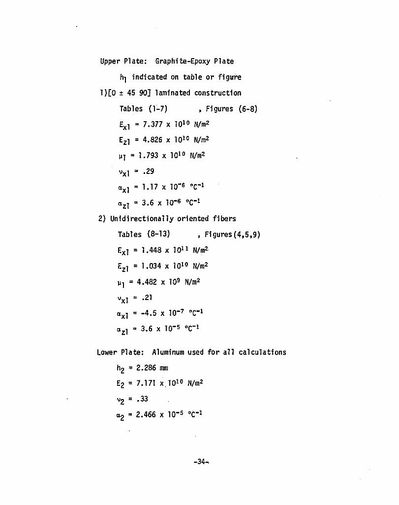
Upper Plate: Graphite-Epoxy Plate

hl indicated on table or figure

1)[0 ± 45 90] laminated construction

Tables (r .. 7) , Figures (6-8)

Exl = 7.377 x 1010 N/m2

Ezl = 4.826 x 1010 N/m2

Pl = 1.793 x 1010 N/m2

"'xl = .29

axl = 1.17 X 10-6 °C-I

azl = 3.6 X 10-6 °C-I

2) Unidirectionally oriented fibers

Tables (8-13) , Figures (4,5,9)

Exl = 1.448 x lOll N/m2

Ezl = 1.034 x 1010 N/m2

ul = 4.482 x 109 N/m2

"'xl = .21

axl = -4.5 X 10-7 °C-I

azl = 3.6 X 10-5 °C-I

lower Plate: Aluminum used for all calculations

h2 = 2.286 mm

E2 = 7.171 x,lOlo N/m2

"'2 = .33

a2 = 2.466 X 10-5 °C-I

-34 ...

Adhesive: typical epoxy

ho indicated on table or figure

1, indicated on table or figure

-t/ e:( t) G(T,t)= {[(~o(T)-~=(T)]e + ~=(T)}H(t) (85 )

the Laplace transform of this is needed for the numerical work

where

G(T,s) ~=(T) -~=(T)

= s+l/e:(T)

e: (T) ~=(T)

= ~o(T)to(T)

~o(T) = lim G(T,t) . t-+O+

~=(T) = lim G(T,t) t~

~=(T) +

s

to(T) is the retardation time

(86 )

(87 )

(88 )

( 89 )

( 90 )

where the numerical values of the constants are as follows. These

values are obtained from [11].

-35-

Table 14

T(OC) Eo(N/m2) llo(N/m2) lloo (N/m"C) to(hours)

21 3.206xl09 1.241xl09 5.516xlOB .5 43 3.034x109 1.172x109 4.826x10B .5 60 2.827.x109 1.089x109 3.999x10B .5 82 2.655x109 1.034x109 3.447x10B .5

6. Fracture of the Bond Edge, Formulation

In this section I will assume the adhesive to behave elasti­

cally. The only changes in the formulation will be in equations

(16) and 08)which will be replaced by

"C = Gy (91 )

(92 )

where the second relation is obtained from plane strain consider­

ations.

From an energy balance of an elastic solid neglecting inertia

forces we have

(93 )

where A is the crack area, U is the \-/ork done by external forces,

V is the stored elastic energy, and YF is the fracture

energy. If fixed grip conditions are assumed the work done

by external forces is ze~ and (93) becomes

-36-

dV _ - dA - YF •

Consider a crack of length da to initiate at the bond edge. The

volume enclosed by this portion of the adhesive is ~ hodA for

unit depth where ho is the thickness of the bond and dA = 2da.

Note that ~ : is then the stored energy per unit volume or simply a .

the strain energy density function evaluated at the bond edge

taking into account that stresses and strains have been averaged

through the adhesive thickness and assuming that all stored energy

is released upon deponding. Note that this assumes a tensile

stress which tends to open the crack. For plane strain the strain

energy density is given by

(95 )

Using Hooke's law to write W in terms of EX' cry and 'xy we get:

E€ 2 cr 2 ,2 _ 1 [x -v 1-,,-2,,2 xy]' W-- __ +.....L- +--2 1;..,,2 E I-~ G

(96 )

Since energy is being released, i.e. force and displacement are

in opposite directions, ~~ is negative and (94) becomes

(97 )

If a crack initiates while the bond edge is in compression then

not all the energy will be released and the term in the strain

-37-

energy density function corresponding to the nonna1 stress

should be ignored. For ay<O we get

ho EE:x2 1'2xy

YF = 4"" [1-,,2 + G] (98 )

It should be noted that in the preceeding analysis the treatment

given to the shear stress is not ve~ accurate. Actually the

shear stress is zero on the free surface and infinite at the

corners. The average value is used which may perhaps be signifi­

cantly low when considering a crack growing from a corner. There

is no way in the present analysis to correct for this.

7. Solution and Results

We want to ca1cu1ate(96)at the end of the bond or say at x=-~.

Therefore we need ay(-~), 1'y(-~) and E:x(-~). The solution for l'

and a is already given. To detennine E:x(-l) note the following.

From equation (8b)

dU1 h1 dS1x dU2 h2 ds2x E:x = (dx - T"dX + dx + T"dX)/2 (99 )

using (4a,ti)with T=To and (5a,b)we get

h1 h2 E:x = [C1 N1 x - T 01 M1 x + C2N2x + "2 02M2x]/2 (100)

evaluating this at X=-l

-38-

(101 )

where N1x{-R.), r41x{-R.), N2x{-R.), M2x{-R.) are given by the boundary

conditions.

It may also be of interest to calculate the geometry of the

"crack", i.e. the displacement (COD) and the rotation. To do

this we need vl{-R.}, v2{-t), B1{-t}, and S2{-R.}. To uniquely

define the displacement field, values of u, v, and B must be spe-

cified at some point. I will choose

Recalling equations {8a} and (92) we may write

1-v-2v2 v

€y = E(l-v) a - 1-v €x = {v1-v2)/ho .

Now solving for v2

ho{1-v-2v2 ) hov v2 = vl - E{l-v) a + 1-v €x

now evaluating at X=-R., taking into account vl{-R.) = 0

( 102)

( 103)

( 104)

ho(1-v-2v2 ) h v v2{-R.) = - E{l-v) o(-R.) + l~v €x{-R.) (lOS)

To determine S2(-R.) recall equation (6b).

-39-

Q2x dV2 62x = B2 - dx

Using (103) we get

( 106)

Q2X· dv 1 ho (1-\1-2\12 ) do h \I dE x 62 =-- {-- =+~-} (107)

x B2 dx E(1-v) uX l-v dx

From equation (6a) we can write

( 108)

The solution for the adhesive stresses in the case of an

elastic adhesive can be found in [1]. They are given as

where all constants are defined in [1]. The only difference

between this solution and the one presented in this study is the

substitution of equations (91) and (92) for (16) and (18). From

(109) we obtain

Using equatjon (100) \'1ith (la,b) and (3a,b) weobtain

-40-

( 112)

Substituting (108), (111) and (112) into (107) and evaluating

at X=-1, we obtain

h (1-v-2v 2 ) a da I EO-v) dx X=-1

( 113)

where

( 115)

Another interesting parameter from a fracture mechanics point of

view is the stretch defined as

a-ho Il = -- where a is the distance from one corner of the bond

ho at adherend 1 to the other corner of the bond at adherend 2.

From simple kinematics

-41-

( 116)

(117)

to get ~(-1.) we note that

€ (-1.) = ___ 1 (vl{-1.) - v2(-1.» Y ho

(118 )

T (-1.) = xy G

Yxy(-1.) (119)

So v2( -1.) 2 1

( 1 - ) + (3.....1 - 1 • ho G

(120 ) ~(-1.) =

The following example \'1as considered for some brief calcula­

tions.

Upper and Lower plate: Aluminum

E = 7.239xl010 N/m2

v = .33 .

AClhesive:

E = 1.931xl09 N/m2

v = .40 ,

ho = .127 mm .

Loading: No = 1.112xl04 N •

The problem considered was the extension 'of a cover plate (see

figure 2g). Values of 1. were varied from 25.4 mm to 254 mm. It

-42-

was found, like the results of tables 8 and 9, that the results

were not dependent on t. The results are

case a) hl = 6.35 mm, h2 = 3.175mm

YF = 36.92 N.m/m2

v2(-t) = 7.562 x 10-~ mm

82(-t) = 9.705 x 10-5

6(-t) = -5.108xlO-;

case b) hl = 3.175mm, h2 = 3.175 mm

YF = 22.6 N·m/m2

v2(-t) ~ 7.184 x 10-5 mm

82(-t) ~ 0

6(-t) ; -5~OxlO-5 .

Recall (102) where the assumption was made that ul(-t) = vl(-t) = 81(-t) = O.

It should be noted that in case a, the bond edge is in com­

pression and that the fracture energy is calculated using equa­

tion (98). In case a the normal stress is very nearly zero.

-43-

Part II

Heat Generation ofa Viscoelastic Material

1. Introduction

Because of the viscoelastic nature of the adhesive and per­

haps also of the adherends, temperature considerations are

important in the design of a bonded joint. Not only do material

properties change with changing temperatures (treated in Part I),

but temperature increases may occur due to viscous dissipation

incurred during loading, especially cyclic loading. This pheno­

menon is illustrated in a test done by Nasa (see figu~ 10) where

at intervals of 10,000 cycles the displacement of a cycling speci­

men is recorded versus time. One observes an increase in the

net displacement and also of the displacement amplitude. Since

the loading stays the same, as seen' on the lower portion of the

graph, the only explanation here is that material properties

change. One parameter that is not recorded in these experiments

is temperature, but this is known to go up due to viscous dissi­

pation as seen from experiments done by the author. The conclusion

is that the dependence of material property behavior or tempera­

ture may be causing the increasing displacement amplitude. The

change in net displacement can be attributed to both temperature

change and to creep.

-44-

From the behavior shown in figure 10, it is evident that

temperature effects are important in design when cyclic loading

of viscous materials exists, a case of which the bonded joint

is a good example. However, the incorporation of these consider­

ations into the analysis of the bonded joint is rather difficult

and therefore will be treated separately in this section.

The problem investigated, both theoretically and experimen­

tally, consists of a one-dimensional specimen subjected to a

cyclic loading at t=O (see figures11a,b). In the theory the

temperature is predicted, in the experiment the temperature is

recorded. The results are then compared. Again, because of

analytical and experimental difficulties, the theory does not

take into account the temperature dependence of material proper­

ties. This limits the solution to temperature ranges over which

these changes are small. The theory also neglects inertia forces,

the effect of which is believed to be small for frequencies con­

sidered in this study. In the solution of the heat equation the

coupling term is included, but its effect is shown to be negli­

gible.

2. Experimental Work

Experiments performed in this study were simple. A plexi­

glas specimen (figure 11a) was cycled in tension on an MTS

-45-

machine at varying frequencies. Temperature measurements were

taken by use of a thermocouple attached at the center of the

specimen and connected to a digital thermometer. A small hole

was drilled in the center of the specimen to accommodate the

thermocouple. The specimen was insulated by cotton wrapped in

aluminum foil. Reinforcement of the specimen was necessary at

the ends, which was accomplished by bonding plexiglas plates of

the same thickness using a solvent cement marketed as IPS Weld-

On 4.

The loading was sinusoidal varying from 1.103 x 107 N/m2

to 3.309 x 107 N/m2. The upper load level is approximately 40%

of the failure load. There was some problem with fatigue cracks

emanating from the drilled hole. This ended the test of the 50

hertz specimen, which appeared to be headed for a range oT pos­

sible melting. The glass transition temperature for plexiglas

is about 72°C. Theoretical results indicate 790C as a~ asymptote.

The recording of the displacement history of the specimen

was not possible at frequencies above about 3 hertz because of

the instruments used. Therefore records like those of figure 10

obtained by Nasa were not possible.

3. Analytical Modeling, Formulation and Solution

An explanation of the phenomenon of rising temperature in

a specimen under cyclic loading is straightforward. As the

-46-

specimen is subjected to load, accompanying strain causes inter­

nal viscous action which generates heat. As one observes the

load-displacement curve through one cycle, a hysteresis loop

shows that there is energy loss equal to the area enclosed.

Several of these loops are shown in figure 12 for varying fre­

quencies. In this study all energy loss was assumed to go

directly into heat. Perhaps some of this energy was expended or

used in some other fonn which may relate to the microstructural

changes in the material, but this was not taken into account.

Perhaps the percentage of dissipated energy that goes into heat

can be taken as a variable, or could indeed be detennined as

being an unknown.

From this basis, for any theoretical study, one needs to

know the displacements in the material under given loads. There­

fore a model must be chosen that describes the constitutive

relations for the material. For this purpose, a spring-dashpot

assembly is chosen as shown in figure 13a.

The problem now consists of three parts. First, a material

characterization must be made. This involves the fitting of an

experimentally obtained creep curve (see figure 14) to the curve

defined by the above chosen constitutive law. The second is

the calculation of the heat input that goes into the energy

equation. The solution of this equation is the third and final

step.

-47-

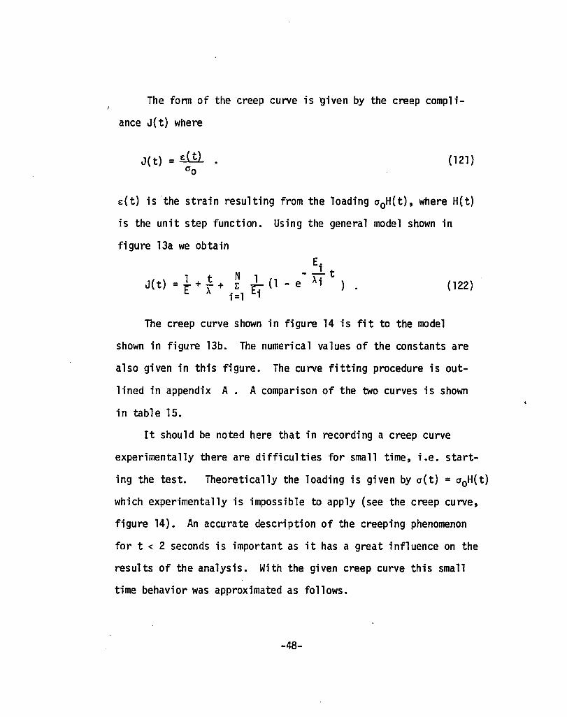
The form of the creep curve is given by the creep compli­

ance J(t) where

J(t) = ll!l . C10 (121 )

e(t) is the strain resulting from the loading C1oH(t), where H(t)

is the unit step function. Using the general model shown in

figure 13a we obtain

J{t)

E. __ 1 t

= El + ; + ~ -El (1 - e Ai ). 1\ i=l i

( 122)

The creep curve shown in figure 14 is fit to the model

shown in figure 13b. The numerical values of the constants are

also given in this figure. The curve fitting procedure is out­

lined in appendix A. A comparison of the two curves is shown

in table 15.

It should be noted here that in recording a creep curve

experimentally there are difficulties for small time, i.e. start­

ing the test. Theoretically the loading is given by C1{t) = C1oH(t)

which experimentally is impossible to apply (see the creep curve,

figure 14). An accurate description of the creeping phenomenon

for t < 2 seconds is important as it has a great influence on the

results of the analysis. With the given creep curve this small

time behavior was approximated as follows.

-48-

In the creep test (figure 14) the data were read directly

from the graph. The problem was that it took about 4 seconds

to increase the load to oo(3.307xl07 N/m2) and during this time

there was significant creeping. It is, therefore, difficult to

determine the initial elastic response which appears to be about

6.4 units on the graph. In the next 4 seconds the specimen

creeps about 0.2 units. It was approximated that during the

first 4 seconds the displacement due to creep would have been

about 0.2 units. Since the average load during the first 4

seconds is half of 00' I estimated the actual creep to be 0.1

unit and that the elastic response was actually 6.3 units.

This is how the values in table 15 are obtained.

A possible improvement to this complication would be to

calculate the response to the loading o(t) = oot H(t), (a ramp

load). This can be applied accurately in an experiment. For

the form of this curve see appendix B. Note that this method

assumes a linear material behavior. In either method the main

problem is the determination of the initial elastic constants.

Another problem often encountered in representing a creep

curve deals with the other extreme of the time scale, the large

time behavior. Usually a creep test is not run long enough to

accurately determine the asymptotic slope of this curve. For

a solid the curve will have zero slope or in terms o~ the model

-~-

of figure l3a, infinite A. A positive slope is characteristic

of a material with fluid behavior. In the problem considered

in this study it was found that the results were not sensitive

to possible val ues of Ai:and that the assumption that plexiglas

was a solid was sufficient.

Given the creep compliance, with the use of the hereditary

integrals, one can find the strain for any loading. The deriva­

tion of this relation can be found in F1 ugge lHJ. . t .

€(t) = aCt) J{O) + J aCt) d~~~:~:~ dt ' . (123) o

The loading in the experiments is given by

aCt) = d + e sinwt • (124)

Substitution of this into (123) gives E. 1 .

N - - t de. d e ( ) d { Ai € ( t) = - + -E s 1 n w t + - t - - cosw t-l + 1: r- 1-e ) E A AW i=l ~i

N + 1:

i=l

An alternate technique for determination of €(t) is given in

appendix c.

-50-

(125)

Before proceding with the derivation let us look at the one­

dimensional energy equation as found in Boley and Weiner 011.

where the subscript A means the stress or strain that is in the

dashpot. K(t) is the bulk modulus, a is the thermal coefficient

of expansion, and To is the reference temperature. The last

term in equation (126) is the coup1 ing term. If we neglect thi s

term, equation (126) has the following more familiar form

( a2T aT Q t) + k 3XT = pc IT ' (127)

where Q(t) is the heat generation term or energy per unit volume

per unit time. It may also be thought of as the rate that

work is done per unit volume. The work done per unit volume is

Again the subscript A is used because the work done in the spring

does not contribute to heating.

The rate at which work is done is

(129)

If this is differentiated we get the terms in equation (1~6).

-51 ..

If we neglect the variation over one cycle and use an' average

value we obtain

(n+1) l'

Q (t) = ~ f a(t)~(t)dt ,

n1'

( 130)

where" is the period and n refers to the nth cycle. The sub­

script A may now be dropped because the integral calculates the

loss through the nth cycle and any elastic contribution will inte­

grate out to zero.

Performing this integration and letting t = 2wn we obtain: III

Q (t) = 1 [e2 + e ~ c. ] + d

2

2 A i=l 1 A

Ei Ei 2 dAi J[ -;q x-:- (t + IIlw) ] +- e - e 1 III Ei 2w '

(131)

where

(132)

The solution of equation (127) with the heat generation Q as given

by (131) has the fonm: (see appendix 0 for solution technique and

boundary conditions)

-52-

N + I:

i=l

b·t e 1 { B· - [ 1

1 b. 1

Wi cosh J~ x - r]) cosh +~

N co

+ I: { I: (2j_1 )nx Sj t

---------- cos e} i=l j=l (2j-1)~[(2j-1)2~2a+bii2]

where

S· - -J

1 e2 d2 e2 N A = [--+-+- I:

2 A A A i=l

W eAi w B· =-[( )2 -1 2~pc E .2+w2A·2

1 1

E· b·

1 1 = - Ai

k a =­pc

A'W2 1

A. 2w2+E.2 ]/pc 1 1

E· 2 1 ~ ---d A' w

(Ei)2]Ei(e 1

R,

(133)

(134)

(135)

- 1) (136)

(138)

(138)

If the coup1 ing tenn is i nc1 uded in equation (126), there is no

point in time-averaging the heat generation, as there is no extra

work involved in taking it as it is. Here an assumption is made

-53-

regarding the bulk modulus K. As in the bonded joint problem, K is

assumed to be time independent. Substituting everythi ng into (126)

and using relations (C2) and (C5) of appendix C we find

N <Xi tN. <Xi t + E A·2A·B·coswte + E Ai2AiCis1nwte

i=l 1 1 1 i=l

N d2 2de e2 + E Ai2BiCisinwtcoswt + - + - sinwt + T sin2wt i=l A A

N N <X1·t (ew ) - 9K<xTo r + E Bi coswt - 9Kc;¥To E Ai e

i=l i=l ( 139)

where

(140)

E·ew 1 B. = 1 A;2w2+Ei 2

( 141)

eA'W2 1 C· = 1 A· 2w2+E·2 1 1

(142)

-54-

( 143)

After expressing time dependent quantities in exponential

form using complex variables, and after defining n~~e constants,

we obtain

\'1here

aT a2T E F iwt B C -iwt -B C pc IT - k a?" = [A + 2 + 2] + e [2i + 2"] + e [2i + 2]

N G· H· (ariw)t + E (.-1. - ..l.) e

j=l 2 2;

d2 d A = - - 9KaTo -

A A

2de . e N B = - - 9KaTo(- + E c,.)

A A ;=1

-55-

(144 )

( 145)

(146)

(147)

or

N E = E >..B.2

. 1 1 1 1=

N e2 F = E >.·C·2 + --

i=l 1 1 >.

N \ I = E >.·2B·Ci . 1 1 1

1=

D. = >.·A·2 1 1 1

G· = 2>. ·A·B· 1 1 1 1

Ji = -9KaToAi

where

E F y = [A + - + -]/pc o 2 2

(-B C) Y2 = 2i + '2/pc

( 148)

(149)

( 150)

(151 )

(152)

(153)

(154)

055)

(156)

(157)

( 158)

-56-

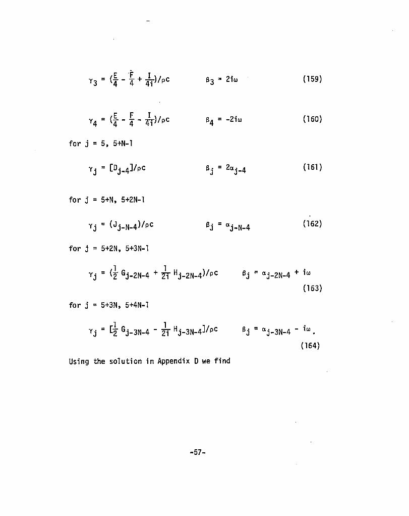
_ E .j: I Y3 - (4 - 4 + 4i)/pC

Y = (£ - E - J..)/pc 4 4 4 <t1

for j = 5, 5+N-1

for j = 5+N, 5+2N-1

for j = 5+2N, 5+3N-1

for j = 5+3N, 5+4N-1

B3 = 2iw ( 159)

(160)

B· = 2cx· 4 J J- (161 )

(162)

B· = cx· 2N 4 + iw J J--(163)

Bj = CXj-3N-4 - iw.

(164)

Using the solution in Appendix 0 we find

-57-

4+4N l3i t e + E Y i -;;--1. [1

i=l ~

f8.i1 coshJ-i- x - ] COShfa ~

(165)

Evaluating this expression at x=O, we obtain the form of the

expression used for the results.

1.2 00

T(O,t) = T + Yo -- + E o 8a n=l

4+4N l3i t 1 + E y i _e_ [1 - fO •

'

]

i=l 13. cosh __ ~1 ~ 1 a 2

4+4N 00

+ E E i=l n=l

4. Discussion of Results

(166)

Before a comparison can be made between theoretical and experi­

mental results, it is necessary to look at the theoretical model­

ing of the experimental results and to justify the choice of the

-58-

parameters used in the theory.

on the following assumptions:

The analytical solution is based

1) heat is generated evenly through-

out ~he domain, 2) the domain is one-dimensional, 3) the ends of

the domain are held at constant temperature for all time, 4) the

specimen is insulated along its length.

It is not possible to satisfy all of these pOints because

there is no well defined length parameter in the experiment. The

geometry of the specimen (figureslla,c) shows that in order to

satisfy "1" and "2" a length of 25.4 mm or 2~=25.4 mm, should be

used. If ~ is chosen larger than this, the width of the specimen

is not constant and therefore the heat generation, which is inversely

proportional to the square of the width, is not uniform. (This

inverse relationship can be seen from equation (131) taking into

account the inverse dependence of stress on width). The boundary

condition T(±~,t) = Tinitial (i.e., the assumption 3), is not

satisfied for 2~ = 25.4 mm but despite this, this value' of twas

chosen for the analytical solution. The affect of this on the com­

parison of solutions should be for the predicted temperature to

be lower than the experimental value due to heat being conducted

out more readily. One compensation here is that the insulation

in the experiment is not perfect, as assumed in the theory, and

therefore escaping heat in the experiment would tend to bring the

two curves closer together.

-59-

The other remaining parameters to be defined are material

properties. Besides the creep curve constants shown in figure

13b, numerical values chosen for the thermomechanical constants

of Plexiglas (polymethylmethacrylate) are:

Bulk Modulus K = 2.382xl09 N/m2

Thennal Diffusivity a = .L = .001276 cm2 sec-1 pc

Thermal Conductivity k = .00154 Watt cm-1oC-1

Coefficient of Thennal Expansion a = .0000goC-1 •

The thermal properties were obtained from [15]. It was

assumed that the bulk modulus was time independent. This made

it analytically possible to include the coupling term.

It should be mentioned that the fourth component in the

spring-dashpot model (figure 13b) contributes almost all of the

generated heat. This is the component that describes large creep-

in9 initially. An accurate determination of its constants E4 and

A4 depends on accurate small time creep readings, which are hard

to obtain as previously discussed. The main difficulty appears

to be in separating the initial elastic response from the small

time creep behavior.

The theoretical results compare very well with the experimen­

tal curves (see figures 15, 16, 17, 18). Because of the discrep­

ency in the boundary condition ;T(±1,t) = Tinitial' the curves

were not expected to be so close. One factor that has a great

-60-

influence on the comparison is the choice of the thermal constants.

There was a range reported in the literature created by the work

of two or three researchers. It is possible that more favorable

constants could have been used. For example, a larger value of

the thermal conductivity would have lowered the asymptote in the

theoretical curves.· Perhaps the most impressive part of the solu­

tion is the functional dependence on 00, shown separately in figure

19 where temperature is plotted as a function of time (19a) and

number of cycles (19b). Here it should be noted that for large

values of 00 where there are great changes in temperature, the solu­

tion becomes less valid because the material properties were taken

to be temperature independent. Initially, however, the solution

is valid for any frequency until inertia forces become important.

The frequency level at which such effects must be taken into con­

sideration may be approximated by the n~tura1 frequency of the

material which is much higher than values in this study.

A comparison was made between the three different theories

used in solving the heat equation. The simplest theory time­

averaged the heat generation per cycle (equation (127) using (131)

as the heat input). The solution was also obtained for the actual

heat generation (equation (126) without coupling), and a third

solution included the coupling tenm (equation 126). It was found

that time averaging the heat generation per cycle is sufficient

-61~

for the temperature profile (see tables 16, 17). If the details

of the temperature are desired through a single cycle then one

must include the coupling term but this effect seems to be rather

insignificant (see tables 18, 19). Boley and Weiner note that

a solution like the one obtained here involving thermoelastic dis­

sipation, is meaningless without the inclusion of the coupling

term. For the specific example solved here, this proved not to

be true [14].

5. Concl usi ons

From the experiments performed, it is evident that temperature

rise due to viscous dissipation is a significant factor in design.

The analytical modeling of this phenomena, although not perfect

because of the difficulties with the small time creep curve, has

proved to work reasonably well. It shows for one thing that time­

averaging the loss over one cycle is sufficient.

The small time creep curve can actually be obtained from the

results of the temperature curve. All that is needed is the ini­

tial slope of the temperature curve. The relationship for small

time is

-62-

e>'iw2

E·2+>..2w2 1 1

(167)

For the example solved in this study, the fourth component of the

spring-dashpot dominates the right hand side of this expression.

As a further approximation we can write

2, 2 aT :: 1 e /\41.1)

pc - - - • at 2 E42+A421.1)2

(168)

If two curves are available for two different frequencies,

I a good guess for E4 and A4 can be obtained by the above formula.

Because of the dominance of the fourth component of the ,

model, it was al so found that the argument whether the material

is a solid (A~) or a fluid (A<=) is unimportant. In many cases

the creep curve can not be run long enough to see if the curve

reaches an asymptote in which case the material is a solid. It

has been found that the value of A does not influence the temper­

ature profile too much and therefore a creep test need not be

run for a long time.

-63-

T=210C xl R. t=O t=5 min. t=20 min. t=l hr. t=3 hr.

T(x,t)/(Mo/s2) -1.0 .651E+03 .579E+03 .455f+03 .38 ItE+O 3 .377E+03 -.98 ... 17[+03 .381E+03 .316F+03 .27?E+tl3 • 26~E+03 -.94 .124[+03 .126E+03 • 12ftf+0! .117E+03 .115[+03 -.90 .517E'+01 .160E+02 .331E'+02 ."01E+02 ."397F+Oc -.80 -.251E+02 -.197E+02 -.891[+01 -.9Q8E+00 -.128f+00 -.70 -.951[+01 -.790E+01 -.r.13F+01 -.30 "E+O 0 • 4"7E'+OO - .60 -.3 .... £+01 -. '30 iE+ 0 1 -.174E+Ol .692E-01 .606E'+00 -.40 -.524F+OO -.527E+00 -."25E+00 -.559£-01 .161f+00 -.20 -.834£-01 -. 97"E-0 1 -.111f+00 -.622E-01 -. '302E-02 0.00 -.288E-01 -.436E-01 -.848f-01 -.146E+OO -.168E+00

.20 -.108£+00 -.163E+00 -.317(+00 -.5C;7~+OO -.664E+00

.40 -.691E+00 -. 9? 8£+00 -.151E+01 -.223~+01 -.24f.f+01

.60 -."49[+01 -.534E'+01 -.715E+C1 -.879E+01 -.910E+01

.70 -.115E+02 -.128E+02 -.154E+02 -.173E'+02 -.175E·02

.80 -.290E+02 -.304E+02 -.327f+02 -.337E+02 .... 336£'+02

.90 -.679£+02 -.671E+02 -.648E+02 -.621E'+02 -.f14f+02

.94 -.917£+02 -.887E+02 -.824£+02 -.771E+02 -.761[+02

.98 -.124E+03 -.117E+03 -.10"E+03 -. 9~ OE+O? -.937F+02 1.00 -.148E'+03 -.137£+03 -.118E+03 -.106E+O~ -.105E+03

o(x,t)/(Mo/s2 )

-1.0 -.206E+04 -.202E+04 -.195E+04 -.lQ2E+04 -.192E+04 -.98 -.686£+03 -.692£+03 -.701f+03 -.708[+03 -.70Q[+03 -.94 • 25 OE+O~ .241E+0~ .224f+03 • 214[+O~ .213E+03 -.90 .291£+03 .29 3E+03 .297£+03 .300£+03 .300E+03 -.80 .490E+02 .507E+02 .544f"+02 .576E+02 .581E+02 -.70 .336f+01 • 262E+0 1 .128E+01 .512[+00 .505E+00 - .60 . • 729E+00 .396[+00 -.312E+00 -.912E+00 -.991E+00 -.40 .170E+00 .155E+ 00 .993f-Ol -. 2q OE-03 -.344£-01 -.20 .252E-01 • 258E-0 1 .203[-01 -.380E-02 -.198E-01 0.00 -.125E-02 -.343E-02 -.114E-01 -.290E-01 -.'t02E-01

.20 -.336E-01 -.46 8E-0 1 -.804f-01 -.124E+00 - .14 OE+ 0 0

." 0 -.222E+00 -. 274E+ 00 -.388E+00 -.~94E+OO -.513[+00

.60 -.143E+01 -.155E+01 -.176E+01 -.186E+Ol.-.1~5E+Ol

.70 -.387E+01 -.395E+01 -.402F.+01 -.393E+01 -.387f+01

.80 -.126E+02 -.124E+02 -.118f+02 -.112E+D2 -.110E+02 .90 -.298E+02 -.280E+02 -.248E+02 -.228E+02 -.22fE+02 .94 -.106£+02 -.857E+01 -.529F.+01 -.383E+01 -.382E+01 .98 .955E+02 • 923E+0 2 .861E+02 .81 6E+0 2 .809[+02

1.00 .221E+03 .209E+03 .168E+03 .175[+03 .174F+03

Table 1. Adhesive stresses for a single lap joint subjected to bending (MoIO, Q~=No=~T=O) for T=2loC, 43°C, 60°C, and 82°C, where hl=. 62mm, h2=2.286mm, ho=.1016mm, R.=12.7mm, and S=2.54xlO-2m.

-64-

T=43°C Xli t=O t=5 min. t=20 min. t=l hr. t=3 hr.

T(x,t)/(Mo/S2)

-1.0 .628E+03 .549E+03 ."18E+03 .350E+03 .~44E+03

-.96 .406E+0'3 .366E+03 .295E+03 .253E+O'3 .248E+03 -.94 .125E+03 .126E+03 .123(+03 .114E+03 .112E+03 -.90 .683E+Ol .204E+02 .376E+02 .4~2E+02 .425E+02 -.80 -.237E+02 -.174E+02 -.551E+01 .248£+01 .313E+01 - .70 -.912E+Ol -. 716E+0 1 -.269E+01 .154E+01 .223E+01 -.60 -.334£'+01 -.276£+01 - • 112E·+01 .105E+01 .160E+01 -.40 -.532E+00 -. 517E+0 0 -.332E+00 .197E+00 .460E+00 -.20 -.891e:-01 -.103E+0 0 -.106E+00 -.lG1E-01 .6G4£-01 0.00 -.338E-Ol -. 533E-0 1 -.107E+00 -.185E+0 0 -.210E+00

.20 -.126£+0{) -.198£+00 -.402f+00 -.116E+00 -.843E+00

.ltO -. 770E +00 -.1(17E+0 1 - .179£'+01 -.266E+01 -.291E+01

.60 -.478f~01 -.578E+Ol -.787£+01 -.966E+01 -.995E+01

.70 -.120f+02 -.135E+0 2 -.163E+02 -.182£+02 -.184E+02

.80 -.295E+02 -.310E+02 -.333E+02 -.341E+02 -.33<lE+02

.90 -.676£+02 -.665E+02 -.637E+02 -.606E+02 -.599£+02

.94 -.906£+02 -.871E+02 -.800E+02 -.743€+02 -.732E+02

.9~ -.122E+D3 -.114£+03 -.996£'+02 -.903£+02 -.890£+02 1.00 -.144E+03 -.132E+03 -.112E+03 -.100E+03 -.989E+02

a(x,t)/(Mo/s2 )

-1.0 -.202E+04 -.197E+04 -.190E+04 -.187E+04 -.187£+04 -.98 -.686E+03 -. 6~ 2E+ 03 -.701E+03 -.707E+03 -.708E+03 -.94 .241E+03 .230E+03 .211£+03 .201E+03 .201£+0'3 -.90 .290f+03 .292E+03 .296E+03 .2~~£+03 .298E+03 -.80 .505E+02 .527E+02 .571E+02 .GOGE+t12 .611E+02 -.70 .319E+Ol • 237E+0 1 .976£+00 .32UE+OO .351E+00 -.60 .607E+00 .207E+00 -.615£+00 -.125E+01 -.131E+01 -.ltO .167E+00 .145E+00 .678£'-01 -.56£.£-01 -.917E-01 -.20 .258E-01 .253E-01 .145£-01 -.214£-01 -.!t13E-01 0.00 -.190£-02 -.507E-02 -.167E-01 -.420E-01 -.565E-01

.20 -.379E-01 -.5lt6E-01 -.970r-01 -.151E+110 -.168E+00

.It 0 -.240£+00 -.302E+DO -.431t£+00 -.5491:+00 -.566E+00

.60 -.147E+01 -.160E+01 -.182£+01 -.190E+01 -.188£+01

.70 -.391E+01 -.399£+01 -.403£+01 -.388£+01 -.381(+01

.80 -.126£+02 -.123£+02 -.117£+02 -.109E+02 -.107E+02

.90 -.289E+02 -.270E+02 -.235£+02 -.215E+02 -.213£+02

.~4 -.93:3E+01 -.713E+01 -.381£+01 -.255E+01 -.258£+01

.96 .941E+02 .90ltE+02 .836F+02 .789£+02 .782£+02 1.00 .215E+OJ .20 lE+ 0:3 .179E+03 .16 7E'+0 3 .165£"+03

Tab le l. Continued

-65-

T=60°C

xh. t=O t=5 min. t=20 min. t=l hr. t=3 hr.

dx, t)/{Mo/s2 )

-1.0 .599[+03 .50 9E+ 03 .3701:+03 .307£+0~ .303£+03 -.98 .392[+03 • 3 .. 5E+ 03 .268£+03 .226[+0~ .223F+03 -.94 .127[+03 .126E+03 .120[+03 .108[+03 .106[+03 -.90 .133f+l'2 .260£+02 ."30E+02 ."63£+02 • "53E+02 -.80 -.218£+02 -.1"3E+02 -.702f+00 .70 3E+ (11 .73't£+01 -.70 -.855E+01 -.6D2E+Ol -."66[+00 .419E+01 • Zt73E+01 -.60 -.317[+01 -.235E+01 -.8Zt5£-01 .259E+01 .311f+01 -.40 -.5351:+00 -. ft82E+OO -.13"[+00 .673E+00 • 989E+0 0 -.20 -.961£-01 -.10 8E+0 0 -.8"lf-Ol .910E-Ol .209E+00 0.00 -.413E-01 -. 692E-0 1 -.1"7f+00 -.250E+00 -.275E+00

.20 - .153f+00 -.25 6E+0 0 -.551[+00 -.9QO[+OO -.11,.[+01

.40 -.882E+00 -.128E+01 -.225[+01 -.33"E+01 -.361E+01

.60 -.517£+01 -.6,.3£+ 0 1 -.89Ztf+Ol -.109E+02 -.111F+02

.70 -.126£+02 -.144E+0 2 -.176f+02 -.1Q5E+02 -.195E+02 • e (I -.302E+02 -.318£+02 -.341F+02 -.345£+02 -.3,.2[+02 .90 -.672f+02 -.657f+02 -.620[+02 -.583E+02 -.575F+02 .94 -.e92E+02 -.8"8E+02 -.764£+02 -.702E+02 -.692E+02 .98 -.116£+03 -.109E+03 -.~34E+02 -.839£+02 -.827[+02

1.00 -.139[+03 -.126E+03 -.104[+03 -.922E+02 -.910E+02

a{x,t)/(Mo/s2 )

-1.0 - .196[+04 -.191E+04 -.183f+04 -.181£+04 -.181£+04 -.98 -.E85£+03 -. 691E+ 03 -.700£+03 -.706E+03 -.707E+03

-.9" .228E+03 .215£+03 .194f+03 .185E+03 .184[+03 -.90 .288E+03 .290E+03 .294E+03 .295E+03 .2'35E+03 -.80 .525[+02 .55"E+02 .609[+02 • 648E+02 .653E+02 -.70 .298E+01 .20 6E+ 0 1 .6,.OE+00 .188[+00 • 266E+0 0 -.60 ."37E+00 -.698E-Ol -.106E+01 -.171E+Ol -.174E+01 -.40 .161£+00 .127E+00 .122[-01 -.1Zt8E+00 -.18 DE +00 -.20 .261E-01 • 233E-0 1 .1"5f-02 -.556E-01 -.803E-01 0.00 -.299E-02 -.810E-02 -.271f-ol -.670E-Ol -.863f-01 .20 - ..... 2E-01 -.669E-01 -.125E+00 -.l~ZtE+OO -.213E"00 .40 -.263£+00 -.342E+00 -.503£+00 -.62 6E+0 0 -.637£+00 .60 -.152E+01 -.167E+01 -.189£+01 -.lQ3E+01 -.189[+01 .70 -.397f+01 -.403E+Ol -.401f+01 -.37 8[+01 -.370[+01 .80 -.126f+02 -.12~+02 -.11Zt£+02 -.105E+02 -.103E'+02 .90 -.27QE+02 -.255E+02 -.217[+02 -.1Q8E+02 -.197£+02 .9ft -.776E+01 -.532E+01 -.199E+01 -.107E+01 -.115E+01 .98 .923E+02 • 879E+0 2 .801E+02 .75 2E +0" • 746E+02

1.00 • 206E'+0 3 .191E+ 03 .167E+03 .156E+03 • 15ZtE+03

Table 1. Continued

-66-

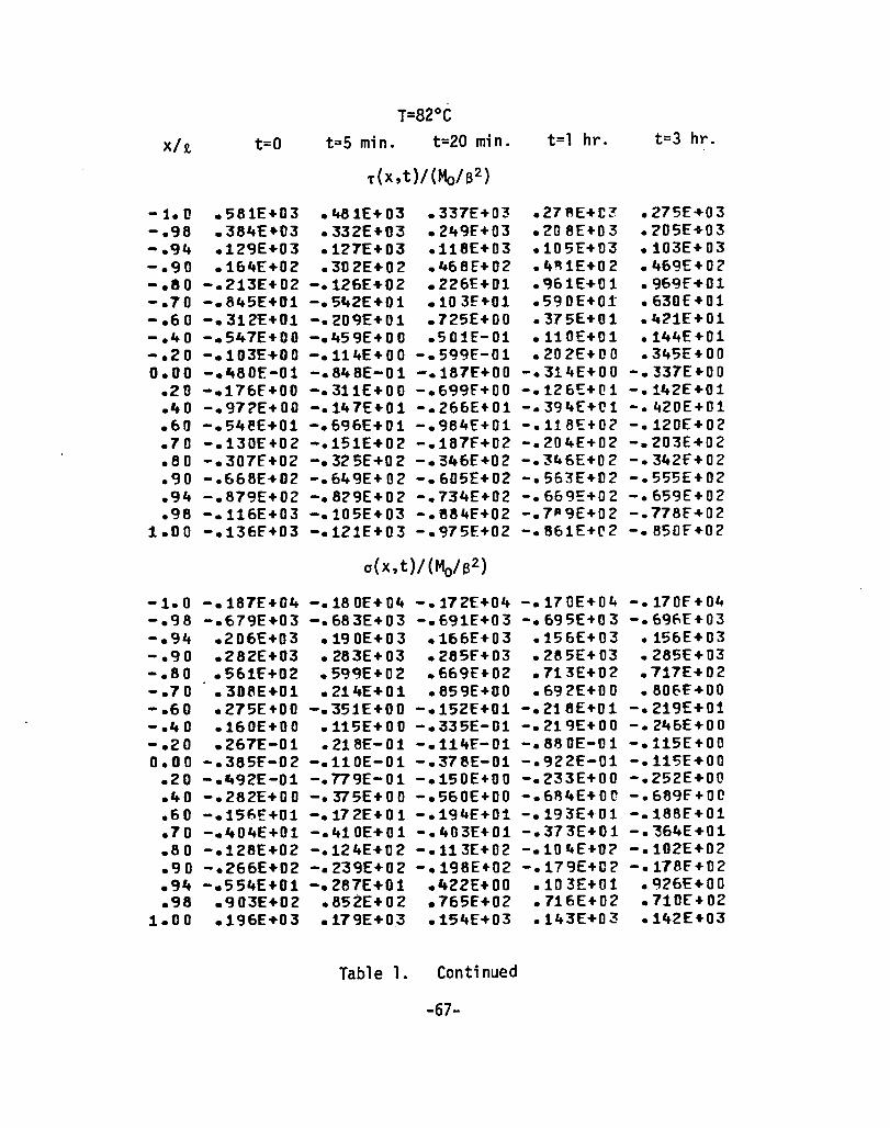
T=82°C

x/R. t=O t=5 min. t=20 min. t=l hr. t=3 hr.

T(x,t)/(Mo/s2)

-1. D .581£+03 • '+a 1£+ 03 .337£+03 .27AE+C::r .275£.03 -.98 .38"£"03 .332E+03 .2"9f+03 .208£"03 .205E+03 -.9" .129E+03 .127E+03 .118E+03 .105£+03 .103E+03 -.90 .164£+02 .302E+02 • "68f+02 .4~1£+02 • .. 69£ + 0 2 -.80 -.213£+02 -.126E+02 .226£+01 .Q61£+Ol .969f+Ol -.70 -.8"5£+01 -.5'+2£+01 .103f+Ol .590E+01 .630£+01 -.60 -.312£+01 -.20QE+Ol .725E+00 .375E+Ol • ~C'1E + 0 1 -."0 -.5"7E+00 -."59E+0 0 .SOlE-Ol .110E+01 .144E+01 -.20 -.103£+00 -.114E+0 0 -.599£-01 .202E+00 .3"5£+00 0.00 - .... 80E-01 -.8" 8E-0 1 -.187[+00 -.314[+00 -.337E"00

.20 -.176f+00 -. 311E+0 0 -.699F+OO -.126£+01 -.1"2£+01

... 0 -.97?£+00 -.147£+01 -.266E+01 -. 3CJ .. [+U 1 -.420E+01 .60 -.5 .. e£+01 -.696£+01 -.984£+01 -.118£+02 -.120[+02 .70 -.130[+02 -.151£+02 -.187f+02 -.204E+02 -.203£+02 .80 -.307[+02 -.32 5[ +02 -.5"6£+02 -.3"6E+02 -.3"2f+02 .90 -.668[+02 -. 649E+ 02 -.605[+02 -.563E+D2 -.555E+02 .9" -.879[+02 -.8C'9E+OC' -.734E+02 -.669£+02 -.659E+02 .98 -.116E+03 -.105E+03 -.!l84f+02 -.7"9E+02 -.778f-+02

1.00 -.136f+03 -.121[+03 -.975[+02 -.861E+('2 -.850f+0C'

a(x,t)/(Mo/S2)

-1.0 -.187[+0" -.180E+04 -.172E+04 -.170E+04 -.170f+04 -.98 -.679£+03 -.683E+03 -.691£+03 -.695£+03 -.69f,[+03 -.94 .206£+03 .190E+03 .166£+03 .156E+{)3 .156£+03 - .90 .282E+03 • 283E+ 03 .285f+03 .285E+03 .285£+03 -.80 .561£+02 .599E+02 .669£+02 .713E+02 .717£+02 -.70 .308E+Ol .21"£+01 • 859£+00 .692E+00 .806[+00 -.60 .275E+00 -.351E+00 -.152[+01 -.218E+01 -.219£+01 - ... 0 .160E+00 .115E+00 -.335E-01 -.219E+OO -.2"6£+00 -.20 .267£-01 • 218£- 0 1 -.114f-01 -.81l0E-Ol -.115E+00 0.00 -.385[-02 -.110E-01 -.378£-01 -.922£-01 -.115[+00

.20 - .... 92£-01 -.779E-01 -.150E+00 -.233E+00 -.252£+00

.40 -.282£+00 -.375E+00 -.560E+00 -.68"E+00 -.689f+OC

.60 -.156E+Ol -.172E+0 1 - .194£+01 -.193E"01 -.188[+01 • 7 0 -."04£+01 -.410E+01 -.403£+01 -. 373E+0 1 -."36"E+01 .80 -.128£+02 -.124£+02 -.113[+02 -.10r.£+0C' -.102E+02 .90 -.266E+02 -.239E+02 -.198E+02 -.179E+02 -.178f+02 .9" -.554E+01 -.287E+01 .422E+OO .103EHll • '126£+00 .98 .903£+02 .852E+02 .765[+02 .716E+02 .710(+02

1.00 .196£+03 .179£+03 .154£+03 .1lt3E+03 .142E+03

Table 1. Continued

-67-

1

T=2l0C

xlR. t=O t=5 min. t=20 min. t=l hr. t=3 hr.

-r(x,t)/(N0i3)

-1.0 -.476£+02 -. "25£-+02 -.338£+02 -.287£+02 -.283E+02 -.98 -.315E+02 -.289E+02 -.242£+02 -.211£+02 -.207E+02 -.94 -.113£+02 -.113E+02 -.110£+02 -.103£+02 -.102£+02 -.90 -.270E+01 -.337E+01 -.442E+Ol -.478E+01 - .473£+01 -.80 .629£+00 .22 5E+0 0 -.555E+OO -.111£+('1 -.116E+01 - .70 .221E+OO .697E-Ol -.266£+00 -.582E+O(1 -.639£+00 -.60 .£:.83E-01 .106E-01 -.135E+00 -.31t!E+OO -.356£-+00 -.40 .102E-01 .208£-02 -.250E-01 -.7Jt6E-01 -.972£-01 -.20 .156£-02 .427£-03 -.460£-02 -.116E-01 -.267£-01 0.00 .675E-OJt -.204£-03 -.149E-02 -.544E-02 -.906£-02 .20 -.112£-02 -.174£-02 -.361£-02 -.710E-02 -.C340f-02 .40 -.755£-02 -.102E-Ol -.169E-Ol -.253£-01 -.283£-01 .60 -.491E-Ol -.588E-01 -.797f-01 -.969£-01 -.103E+00 .70 -.125E-+00 -.141£+00 -.172E+00 -.1'~5E+OO -.197£+00

.• 80 -.316E+00 -.334£+00 -.364£+OC -.37 8E+tl 0 -.378£+00 .90 -.766£-+00 -.761E+00 -.743f+00 -.715F+00 -.707f+00 .94 -.108E+Ol -.105E+Ol -.978E+00 -.915£+OC -.903["+00 .98 -.156£+01 -.147E+0~ -.130E+Ol -.118£+01 -.116£+01

1.00 -.193£+01 -.178£+01 -.152£+01 -.135E+01 -.133E+01

a(x,t)/(No/S)

-1.0 .127£+03 .124£+03 .120£+03 .119£+.03 .119£+03 -.98 ."15£+02 • Jtl 9E+ 02 .428£+02 ."33£+0? • "34£+02 -.94 -.160£+02 -.154£+02 -.144£+02 -.138£+02 -.138£+02 -.90 -.179£+02 -.182£+02 -.185E+02 -.18A£+02 -.188£+02 -.80 -.276E+Ol -.286E+01 -.314£+01 -.337E+01 -.341E+01 - .70 -.8"9£-01 -.335£-01 .567E-01 .103E+00 .102£+00 -.60 .204£-02 .280£-01 .815E-01 .124£+00 .129£+00 -.40 -.335E-02 -.599£-03 .696£-02 .171E-01 • 199E-Ol -.20 -.518E-03 -.137£-03 .125E-02 .403£-02 .535E-02 0.00 -.136£-03 -.116£-03 ....... £-04 .606E-03 .105£-02

.20 -.387£-03 -.530E-D3 -.867E-03 -.119£-02 -.117£-02

... 0 -.243£-02 -.302E-02 -.432E-02 -.551£-02 -.568£-02

.60 -.158£-01 -.172E-Ol -.199E-Ol -. 213E-0 1 -.212E-01

.7D -.422E-01 -.43"£-01 -.~"7E-D1 -.""OE-01 -."~3E-01

.80 -.122E+00 -.119E+00 -.111E+00 -.102E+DO -.100E+OO

.90 -.217£+00 -.197E+00 -.159f+00 -.135£+00 -.132E+OO

.94 -.182£-01 .930E-03 .309£-01 .435£-01 .433£-01

.98 .796£+00 .758E+00 .68bE+00 .632£+00 .624£+00 1.00 .166E+01 .154f+Ol .133f+01 .120£+01 .118E+01

Table 2. Adhesive stresses for a single lap joint subjected to axial loading (No~O, Qo=Mo=6T=O) for T=2loC, 43°C, 60°C, and 82°C, where hl=.762mm, h2=2.286mm, ho=.1016mm, i= l2.7mm, and S=2.54xlO-2 m.

-68-

T=43°C Xli t=O t=5 min. t=20 min. t=l hr. t=3 hr.

T(x,t)/(Nrk)

-1.0 -.460E+02 -.404[+02 -.312[+02 -.263[+02 -.259E+02 -.98 -.307£+02 -.27 A£+ 02 -.227f+02 -.196£+07 -.193E+02 -.94 -.113£+02 -.113E+02 -.108£+02 -.100[+02 -. 983f + 01 -.90 -.293£+01 -. 305E+0 1 -.467f+Ol -.493[+01 -.486f'+01 -.eo .518£+00 .582E-Ol -.800[+00 -.135[+01 -.138[+01 -.70 .179£+00 -.169E-02 -.393[+00 -.135[HIO -.786f+00 -.60 .515£-01 -.20AE-01 -.201£+00 -."05E+00 -.451F+00 -.40 .792£-02 -.34 2E-0 2 -."09E-Ol -.100£'+00 -.133f'+00 -.20 .126[-02 -.529E-U3 -. B2P.[- 02 -.275[-01 -.396£-01 0.00 -.546£-05 -.449E-03 -.254£-02 -.6~1[-02 -.141[-01

.2U -.132£-02 -.216E-02 -.473E-02 -.90QE-02 -.129[-01

... 0 -.843E-02 -.118£-01 -.201r-01 -.31)"[-01 -.339f-01

.60 -.524£-01 -.039£- 01 -.881f-Ol -.10 Q[+O 0 -.113[+00

.70 -.131E+00 -.149E+00 -.183f+OO -.200[+00 -.208F+OC

.eo -.323E+00 -. 3ft 2E + 00 -. 373E+0 0 -.3RIJ[+[)(! -.38~[+Or

.90 -.764£+00 -.757E+00 -.732£+00 -.69QE+C[1 -.691E+00

.9" -.107E+01 -.103E+01 -. 950E+ 00 -.681£+00 -.869F.+OO

.9A -.153[+01 -.1"3£+01 -.124[+01 -.112£+01 -.110E+Ol 1.0(1 -.187£+01 -.171E+01 -.143E+Ol -.127£+01 -.121)£+01

a(x,t)/(No/S)

-1.0 .124E+03 .121E+03 .117[+03 .116[+03 .116[+03 -.98 ."15£+02 .420£"+02 • "'26[+02 .4~4[+O2 .435E+02 -.94 -.154E+02 -.147E+02 -.136f+02 -.131E+02 -.130£+02 -.90 -.179E+02 -.181£+02 -.165E+02 -.187[+02 -.187E+02 -.80 -.285£+01 -.301£+01 -.332[+01 -.35"£+01 -.362[+01 -.70 -.719E-Ol -.159[-01 .765f"-01 .114£+00 .110E+00 -.60 .115E-01 • 422E- 01 .103£+00 .14"£+00 .151E+00 -.4.0 -.256E-02 • 996E- 03 .106£-01 .226£-01 .253£-01 -.20 -.414[-03 .138£-03 .212£-02 .564£-02 .738[-02 0.00 -.134E-03 -.900£-04 .188f-03 .105E-02 .166[-02

.20 -.435E-03 -.611E-03 -.101E-02 -.133E-U2 - .123E-02

.40 -.263£-02 -.33 "£-02 -.464E-02 -.611E-02 -.621[-02

.60 -.163£-01 -.179[-01 -.207[-01 -.21QE-(,1 -.216[-01

.70 -.427[-01 -.439£- 01 -.4"9£-01 -.435[-01 -.427E-Ol

.80 -.121£+00 -.118£+00 -.108E+00 -.Q82E-Ol -.961£-01

.90 -.208[+00 -.185£+00 -.145[+00 -.121E+00 -.119£+00

.94 -.769E-02 .126£-01 .425£-01 .5~7[-O1 .521£-01

.98 .781£+00 .738£+00 .658[+00 .602£+00 .594£+00 1.00 .160£+01 .1 ... 7E+01 .125[+01 .112[+01 .111£+01

Table 2. Continued

-69-

T=60°C

xl! t=O t=5 min. t=20 min. t=l hr. t=3 hr.

T(x,t)/{Nob)

-1.0 -.1t39E+02 -. 376E+0 2 -.278E+02 -.232E+02 -.229E+02 -.98 -.297£+02 -.263E+02 -.207£+02 -.177£+02 -.174£+02 -.94 -.114E+02 -.112E+02 -.105E+02 -.95 2E +01 -. g34f+01 -.90 -.321£+01 -. 398E+0 1 -.497E+Ol -.505E+Ol -.495f+Ol -.80 .374E+00 -.176E+0 0 -.114E+01 -.166E+Ol -.167E+01 -.70 .121£+00 -.107E+0 0 -.583E+00 -.951E+00 -.988E+00 -.60 .272E-Ol -.700E-Ol -.306£+00 -.548'£+OC -.591£+00 -.40 .421£-02 -.132E-Ol -.699F'-01 -.1S?E+Ofl -.194E+OC -.20 .706E-03 -.244E-02 -.158£-01 -.,,71£-01 -.641E-Ol 0.00 -.1,+7£-03 -.961E-03 -.'+83E-02 -.161E-Ol -.2,+7F-01

.20 -.163£-02 -.287E-02 -.685£-02 -.14~E-0·1 -.199E-01

.40 -.970E-02 -.1'+2E-Ol -.254£'-01 -.388£-01 -.432£-01

.60 -.569£-01 -.713E-01 -.101E+00 -.124E+00 -.127E+00

.70 -.138E+00 -.159£+ 0 C -.198£+00 -.221 E+ 0 (1 -.222E+00

.80 -.331E+00 -.352E+OO -.383E+00 -.39 1E+ 0 0 -.388[+00

.90 -.761E+00 -.75 OE+O 0 -.715E+00 -.675£+00 -.665f+00

.94 -.105f+01 -.101E+01 -.908E+00 -.833[+00 -.822E+OC

.98 -.149E+Ol -.137E+Ol -.116£'+01 -.103[+01 -.102£+01 1.0n -.181f+01 -. 162E+ 0 1 -.132E+01 -.116'£+01 -.115F+01

a(x,t)/(No/s)

-1. 0 .121£+03 .118E+03 .114E+D3 .113E+03 .113E+03 -.98 .415£+02 .42 OE+ O? .429F'+02 .435E+02 .436£+02 -.94 -.1'+6E+02 -.138E+02 -.126E+02 -.120~+O2 -.120£+02 -.90 -.178[+02 -.181E+02 -.184E+02 -.166£+02 -.186£+02 -.80 -.299E+Ol -.319£+01 -.358[+01 -.386E+Ol -.390£+01 -.70 -.566E-01 .577E-02 .978[-01 .119E+00 .111£+00 -.60 .244E-01 • 627E-0 1 .135E+00 .17g[+00 .179F+00 -."0 -.138E-02 .358E-02 .166E-01 .310E-01 .333£-01 -.20 -.237E-03 .64 3E-03 .372E-02 .903[-02 .108E-01 0.00 -.123£-03 -.275E-04 .504E-03 .198E-O~ .282f-02 .20 -.502E-03 -.733E-03 -.122E-02 -.145[-02 -.119E-02 .40 -.290E-02 -.37 9£-0 2 -.562f-02 -.60 0£-02 -.684E-02 .60 -.16Qf-01 -.188E-Ol -.217E-Ol -.2:.'3E-01 -.21QE-Ol .70 -.434E-01 -.445E-Ol -.449f-01 -.424£-01 -.414£-01 .80 -.121E+00 -.116E+00 -.103E+0~ -.919E-01 -.900f-01 .90 -.197E'+00 -.170E+00 -.126E+00 -.10 '3E+OO -.102E+00 .94 .501E-02 .270E-Ol .561E-01 .627[-01 .616f-01 .98 .761£+00 .70 9E+ 0 0 .618E+00 • 561E+ 0 0 .553[+00

1.00 .153E+01 .138E+O 1 .114£+01 .102'£+01 .101£+01

Table 2. Conti nued

-70-

T=82°C

xl! teO t=5 min. t=20 min. tel hr. t=3 hr.

T(x,t)/(Noh)

-1.0 -.426E+02 -.356E+02 -.254E+02 -. 211E+O 2 -.209£+02 -.qe -.291F.+02 -. 253E+0 2 -.193[+02 -.16'3E+02 -.161£+02 -.94 -.115E+02 -.112E+02 - .10 2E+ 02 -.916E+Ol -.900£+01 -.qO -.339£+01 -.423E+01 -.515E+Ol -.509E+Ol -.499£+01 -.80 .324E+00 -.305£+00 -.135£+01 -.1~3£+01 -.182£+01 - .70 .Q74E-Ol -.173E+0 0 -.716E+00 -.1!J~£+01 -.112E+01 -.60 .133£-{)1 -.106E+00 -.390[+00 -.658E+00 -.695£+00 -.40 .180E-02 -.213£-01 -.967E-01 -.212[+00 -.246E+00 -.20 .313E-03 -.421E-02 -.236£-01 -.672E-Ol -."R1F-Ot 0.00 -.261E-03 -.148E-02 -.743E-02 -.245[-01 -.361E-01

.20 -.186E-02 -.355£-02 -.908£-02 -.204E-01 -.274E-01 .40 -.107£-Dl -.164£-01 -.303£-01 -.466E-01 -.51~F-Ol .60 -.604E-01 -.775E-01 -.111E+00 -.135£+('0 -.136E+Oe .70 -.143~+00 -.16R£+00 -.210E+00 -.232f+00 -.232E+00 .80 -.337£+00 -.36.0E+00 -. 391E+0 0 -. 3Q3E+O 0 -.389F+00 .90 -.758E+00 -.743£+00 -.699£+00 -.653E+00 -.644E+00 .94 -.104(+01 -.QR4E+OO -.874E+00 -.795E+OO -.7"3f+00 .91' -.146f+01 -.132£+01 -.109f+01 -.972E+OO -.958F.+00

1.00 -.176f+Ol -.155E+Ol -.123£+01 -.10BF+C1 -.107E+01

o(x, t)/ (No/ B)

-1.0 .115£+03 .111E+03 .107E+03 .106£+03 .106E+03 -.98 ."12£+02 .416£+02 .42'+f+02 • '+2 QE+O 2 .430£+02 -.94 -.133E+02 -.123E+02 -.106E+02 -.102E+02 -.102£+02 -.90 -.175E+02 -.177£+02 -.179£+02 -.18 OE+O 2 -.180£+02 -.eo -.321E+01 -. 3'+6E+0 1 -.397F+Ol -. '+2 9E+0 1 -.432E+01 -.70 -.603E-01 .326£-02 .8'+1E-01 .844E-Ol .740£-01 -.60 • 363E-0 1 .82 8E- 0 1 .166E+00 .209£+00 .208E+00 -.40 -.677E-03 .553E-02 .215E-01 .375E-Ol .391£-01 -.20 -.122£-0~ .107E- 02 .523E-02 .11CJE-01 .136E-01 0.00 -.117E-tl3 .321E-04 .841£-03 .2CJ4E-02 .3CJ5£-02

.20 -.556£-03 -.838E-tJ3 -.139E-02 -.145£-02 -.103E-02

.40 -.311£-02 -.417£-02 -.625£-02 -.7'+3E-02 -.720f-02

.60 -.174£'-01 -.195E-Ol -.224£-01 -.224E-Ol -.218f-01

.70 -."42E-01 -.453£-01 -."50E-01 -.416£-01 -.405F-01

.80 -.121E+00 -.115E+0 0 -.100£+00 -.679E-01 -.861E-01

.«30 -.185E+00 -.154E+OO - .107E+00 -.865E-C1 -.853E-01

.«34 .212E-Ol .445E-01 .718E-01 .746E-01 .734F-01

.98 .741E+OO .662[+00 .582£+00 .524£+00 .517£+00 1.00 .145£+01 .128E+01 .10'+£+01 .921£+00 • CJl0E +00

Table 2. Continued

-71-

T=2l0C X/t t=O t=5 min. t=20 mi n. t=l hr. t=3 hr.

T(X,t)/(Qo/S)

-1.0 -.639E'+03 -.566E+03 -.443E+03 -.372E+03 -.366£+03 - .91' -.405E+03 -. 36 '3£ + 03 -.304E'+03 -.2r,2£+03 -.257E+03 -.94 -.114£+03 -.116£+03 -.114£+03 -.107E+03 -.105E+03 -.90 .337E+01 -.730£+01 -.243£'+02 -.312E+02 -.~08£+02 -.80 .333E+02 • 279E+ 02 .173£+02 .945£+01 .859F+01 - .70 .181£+02 .165£+02 • 12AF;+02 .897£+01 • ~22E.+Ol -.60 .123£+02 .118£+02 .105E+02 .873£+01 .820E+01 -.40 .~45E+Ol .945£+01 .C:-34£+01 .R96E+C1 • fl74E +01 -.2e .C:-03£+01 • 904E+ 01 .904f+01 .697E+01 • SA9E +01 0.00 .696£+01 .896£+01 .897[+01 .896E+01 .893[+01

.20 .e95E+01 .895E+01 .895£+01 .895E+01 .895£+01

.40 .~95E+01 .895£"'01 .895f+Ol • 8~6£+01 • 895E+0 1

.60 .897£+01 • 897E+0 1 .898£+01 .898~+O1 .898E+01

.70 .901E+Ol .901E+01 .901E+Ol .9"0=:+01 .900£+01

.80 .910E+01 .909£+01 .907E+Ol .905£+01· .904f"'01

.90 .903f+01 .901£+ 01 .897E+01 ."95£+01 • P95f+01

.94 .875£+01 .875£+03 .87 6E' + 0 1 .877E+01 .87RE+Ol

.98 .831E+Ol .836£+ 0 1 .846E+Ol .85 ?£+O 1 .853£+01 1.011 .619E+01 • ~26£+01 .638F+Ol .84 6f.+ 0 1 .847E'+01

a (x, t)/-{ Qol B)

-1. 0 .199f.+04 .195E+04 .188E+04 .1~SE+04 .185£+04 -.C?8 .f.49F+O'3 .654£'+03 .664£+03 .671£+03 .672E+03 -.94 -.257E+0~ -. 248E+ 03 -.232£+03 -.22?E+03 -.221£+03 -.90 -.289E+03 -.292E+03 -.296E+03 -.299£+0" -.29Q £"'03 -.80 -.480E+02 -.497£+02 -.533£+02 -.564£+02 -.56QE+02 -.70 -.321E+01 -.247£+01 -.113F+01 -.364:+00 -.357F+00 -.60 -.£:95f+00 -.363E+00 .339E ... 00 .933£+00 .101E+01 -.40 -.164£+00 -.149E+OO -.923E-01 .642E-02 .393£-01 -.20 -.251E-01 -. 261E-0 1 -.220r-01 -.155£-02 .11~£-O1

0.00 -.384E-O? -.453E-02 -.497E-02 -.124'=-02 • 325E-0 2 .20 -.415E-03 -. 566E- O~ -.771£'-03 -.124t-O~ .124E-02 .40 .108E-02 .117f-02 .130E-02 .141£-02 .174E-02 .6 () .697£-02 • 658E- 02 .S46F-02 .411'£-02 .400E'-02 .70 .301E-01 .301E-01 .3etE-0! .2g7E"-Ol .29AF-Ol .60 .203E+00 .213£+ 00 .231[+00 .243E+00 .245E+00 .90 .259E+00 .240E+00 .205E+0!J .185E+UO .184f+00 .94 -.136F+01 -.143E+01 -.154E+01 -.16'1£+"1 -.161£+01 .9E1 -.753E+01 -. 751E+ 01 -.747£+01 -.71.4E+"1 -.744E+01

1.00 -.142E+02 -.139E+02 -.135[+02 -.13?f+02 -. 132F. ... 02 .

Table 3. Adhesive stresses for a single lap joint subjected to transverse shear loading (Qo~O, No=Mo=~T=O) for T=2loC, 43°C, 60°C, and B2°C, where hl=.762mm, h2=2.286mm, ho= .1016mm, t=12.7mm, and S=2.54xlO-2m.

-72-

T=43°C xl! t=O t=5 min. t=20 min. t=l hr. t=3 hr.

T{x,t)/{Qo/a)

-1.0 -.615E+03 -.536E+03 -.407E+03 -.33C3E+03 -.333£+03 -.98 -.394E+03 -.354E'+03 -.284f+03 -.242E+03 -.237E'+03 -.94 -.115E"03 -.116E+03 -.113f+03 -.1nf+E'+I)~ -.102E+0~ -.90 -.244E+OO -.117E+02 -.288f+02 -.342E+02 -.335£+02 -.80 .319£+02 .257£+ 02 .13gE+02 .601~+01 .537[+01 -.70 .177£+02 .158E+02 .113f+02 .713E+01 .645£+ 01 -.60 .122E+02 .116E+02 .99.2f+01 • 775E+0 1 .720E+01 -.40 .946£+01 • 941tE+0 1 .924E+01 .870E+01 .843[+01 -.2C .903E+01 • g04E+01 .903f+01 .8gnE+01 .f!aOE+01 0.00 .~96E+01 .896E+01 .897E+01 .SC34E'+01 .890E+01

.20 .895E+01 .895E+01 .895E+01 .895E+01 .894£+01

.40 .895E+01 .895E'+01 .896F+01 .896E+01 .895£+01

.60 .897£+01 .897£+01 .898£+01 .89PE+t'1 .897E+01

.70 .901£+01 • gO 1£+01 .901f+01 .90 OE+O 1 . • 900F+01

.f! 0 .CJOCJE'+01 .908E+01 .906E'+01 .90ItE+01 .C?04f+01

.90 .902£+01 .900E+01 .896E+Ol .89 4E+0 1 • ~9SF+Dl

.94 .875E+01 .875E+01 .876f+01 • 877E+~ 1 • 87R~+01

.98 .83ZF+01 .838E+01 .848[+01 .855~+01 • a56E +01 1.00 .821E+01 .82 BE+ 0 1 • a41f+01 .850E+Q1 .851f+C1

a{x,t)/{Qo/a)

-1.0 .195E+04 .190E+04 .183£+04 .180£+04 .180E+04 -.9~ .649E+03 .654£+03 .664E+03 .670£+03 .671E+O~

-.94 -.248E+03 -. 237E+ 03 -.219f+03 -.210E+03 -.209E+03 -.90 -.289E+03 -.291E+03 -.295E+03 -.297E+03 -.298E+03 -.80 -.494E+02 -.516E+02 -.559E+02 -.5Q3E+02 -.599E+02 -.70 -.303'E+01 -.221E+01 -.820£+00 -.163£+00 -.195£+00 -.60 -. 572E+0 0 -.175E+ 0 C .641E+00 .127E+01 .133E+01 -.40 -.161£+00 -.139E+00 -.608E-01 .619£-01 .953£-01 -.20 -.258E-01 -.259E-Ol -.172E-01 .132E-01 .295E-Ol 0.00 -.412E-02 -.478£-02 ~.443E-02 .238E-02 .874E-02

.20 -.470E-03 -.633E-03 -.725f-03 .733E-O~ .294E-02

.40 . .113£-02 .123E-02 .136E-02 .160f-OZ • 22E-f-02

.60 .E95£-02 .643£-02 .503E-D2 .357£-02 .~53E-02

.7 (j .311E-01 .313E-Ol .313£-01 .313E-01 .3161:-01

.80 .211E+00 • 222E+ 00 .243£+00 .256£+00 • 257F+OO

.90 .239E+00 .216£+00 .177E+OO .156£+00 .154£+00

.94 -.141E+01 -.149E+01 -.161E+Ol -.107~+01 -. 167E+ 0 1

.98 -.751E+01 -.748E+01 -.743F+01 -.741E+Ol -.74::1£+01 1.00 -.140E+02 -.137£+02 -.132E+02 -.130F+02 -.130E+02

Table 3. Conti nued

-73-

T=60°C xh. t=O t=5 min. t=20 min. ,t=l hr.· t=3 hr.

't'(x,t)/(Qo/S)

-1.0 -.586(+03 -.497E+03 -.359F+03 -.296E+03 -.292£+03 -.98 -.3AOf+03 -.333E+tl3 -.257E+03 -.215£+03 -.212E+03 -.94 -.117E+03 -.116E+03 -.110f+03 -.9P.7E+02 -.965E'+02 -.90 -.468£+01 -.173£+02 -.341E+02 -.372E+02 -.363E'+02 -.80 .300E'+02 .225£+02 .913E+01, .151£+01 • 12D~+01 -.70 .172F+02 .146E+02 .911F+01 • 1t5 OE+O 1 .396F+01 -.60 .120E'+02 .112E+02 .888E+01 .621[+01 .569E+01 -.40 .946£+01 .9'+ OE+ 01 .904f+Ol .621E+(l1 .787E+01 -.2e .904E+01 .90 4f+ 01 .899E+Ol .676E+01 .86 Ol=' + 0 1 0.00 .~96~+01 .897E+01 .896E+01 .890E+01 .884E+Ol

.20 .~95E+01 • 895E+0 1 .895E+01 .894E+01 .891E+01

.40 .e95£+01 .895E+01 .896f+01 .895E+01 .895f'+01

.6 (l .897E+01 .898E+(l1 .898F+01 .898E+!!1 .897£+01

.70 .901£+01 .901E+01 .901E+01 .900£+01 .900£+01

.8 [j .909£+01 .90A(+01 .905E+01 .903E+D1 .903E'+01

.90 .901£+01 .898E+01 .894E+01 .89~E+Ol .893E+01

.94 .874E+Ol .874£+01 .876E+01 .878E+01 .879E+01

.98 .833E+01 .84 OE+ 0 1 .852£+01 .65qE+01 .1300£ +01 1.00 .823E+01 .831E+01 .846[+01 .855F+Ol .e55E+Ol

a(x,t)/(Qo/S)

-1.0 .189E+04 .184£+04 .177E+04 .174£+04 .175£+04 -.98 .648£+03 .654E+03 .664E+03 .670E+0:! • €:71~+0~ -.94 -.236E+03 -.223f+03 -.203E+03 -.1Q4E+03 -.193E+O'3 -.90 -.287E+03 -.290E+03 -.293E'+03 -.295E+O~ -.295E+03 -.80 -.514(+02 -.542E+02 -.596E+02 -.635E+02 -.639£+02 - .70 -.262F+Dl -.190(+01 -.474E+00 -.195E-Ol -.976£-01 -.60 -.403E+00 .101E+00 .108F+01 .172E+01 .175E+01 -.40 -.155E+00 -.120E+00 -.532E-02 .151£+00 .181F+00 -.20 -.263£-01 -.244[-01 -.634E-02' .417E-t)! .611E-01 0.00 -.445E-02 -.49 2E- 0 2 -.257:-02 .107:E-01 .200E-Ol

.20 -.541£-0'3 -.700E-03 -.410E-03 .31.:'7£-02 .692E-02

.40 .120E-02 .130E-02 .146f-02 .219£-02 .358f'-02

.60 .E>88E-02 .614E-fJ2 .429[-02 .275E-02 .307E-02

.70 .325£-01 • 329E- () 1 .334E-01 .3~9E-1l1 .344F-01

.80 • 221E'+0 0 • 235E+ CO .259E+00 .212F+OO .27'3£+00

.90 .213E+00 .184E+00 .137E+00 .115£+00 .115£+00

.94 -.148E+Ol -.157E+(31 - .170E+01 -.175E+01 -.175£+01

.98 -.748E+Ol -. 7lt4£+ 0 1 -.738f+01 -.7?5E+01 -.735E+01 1.00 -.137E+02 -.13ftE+02 -.128E+02 -.12f,£+02 -.126£+02

Table 3. Continued

-74-

T=82°C Xli t=O t=5 min. t=20 min. t=l hr. t=3 hr.

L ( x, t) I (Qol a)

-1.0 -.568f+03 -. 4f. 9E+ O~ -.326£+03 -.2F7E+C3 -.264~+03 -.ge -.372[+03 -.32 OE+ 03 -. 238E+0~ -.1Q~E'+C3 -.195£+0~ -.9" -.119E+03 -.117E+03 -.108E+03 -.950E+O? -. 0.30E +0 2 -.90 -.770£+01 -.214E+02 -.377£+02 -.390f+02 -.379£+02 -.80 .?95E+02 .209£+02 .619f+01 -.11)5E+01 -.112E+01 -.70 .170f+02 .140£+ 0 2 .760[+01 .27I3E+01 .23flE'+01 -.60 .119E+02 .109£+02 .806[+01 .50 4E'+0 1 .457E+01 -.40 .C347E'+Ol .937E+01 .884E+01 .776E+(11 .73<?~+Ol

-.20 .904E+01 .904£+01 • 89~E+01 .eC:-OE+Cl .840E'+01 0.0[1 .P96E+Ol .897E+Ol .896£+01 .8R5£+01 .876£+01

.20 .~95E+01 • 895E+ 01 .895[+01 .893E+01 .888f+Ol

.40 .P.95E+1)1 .896E+Ol .896£+01 .895£+01 • a93f+01

.60 .fg8F+01 .898E+01 .898£+01 .898f+C1 .897f+01

.70 .':!02E+Ol .902E+01 .C!OlE+01 .900~+O1 .8<;!C?F+01

.80 .910E+01 .908£+01 .905E+01 .902E'+01 .902[+01

.90 .900E+01 • 897E+0 1 .893E+01 .a92E+01 .892E+01

.94 .873£+01 • 873E+0 1 .875E+01 .87~E+Cl • ~7eE+01

.ge .833F+01 .841£+(11 .854f+01 .8E-l£+C~ .8tJIE+01 1.00 .823£+01 • 832f+C 1 .f49E+Ol .R57E+Ol .858£+01

a(x,t}/(Qo/a}

-1. 0 .180£+04 .174£+ 04 .166£+04 .164E+04 .164[+04 -.98 .642£+03 • E4 7E+ O~ .E54E+03 .659[+03 • E60E+ 03 -.94 -.214f+03 -.198E+03 -.175E+03 -.166E+0~ - .165£+03 -.9U -.282E+03 -.283E+C3 -.284f+03 -.2R5E+03 -.285E+03 -.80 -.549E+02 -.586E+02 -.655E+02 -.698E+Oc -.702E+02 - .70 -.290=+01 -.195F+C1 -.£:63E+00 -.4C10E+OQ -.603E+OO -.60 -.23~E+00 .31\2E+00 .154E+01 .219£'+01 .21QE+01 -.ftO -.153E+00 -.107E+(10 .'*02£'-01 .21 QE+t10 .244£+00 -.20 -.271)f.-01 -.234E-01 .416E-02 • &79E-01 .882£-01 0.00 -.476~-02 -.502E-02 -.361E'-03 .19AE-01 .313£-01

.20 -.f.OOE-03 -.744E-03 .589E-04 .6~1E-02 .114~-01

.40 .128f-02 • 14t:!E-02 .163E-02 .306E-02 .531f-D2

.60 .706E-02 .610E-D2 .381E-02 .23SE~02 .312f-02

.70 .362£-01 .374E-01 ."394£-01 .410F-Ol .418f-01

.80 .237E+00 .255£+ 0 0 .283£+ 0 0 .297E+OO • 299E +00

.90 .162E+00 .122E+0 0 .608E-01 .3€>?E-01 .356E-01

.94 -.1S9E+01 -.169E+01 -.183E+Di -.i8!\E+Oi -.18eE+01

.9a -.741f.+01 -.736E+01 -.728E+Ol -.725E+tH -.725E+01 1.00 -.133E+02 -.128£+02 -.123[+02 -.121E+02 -.121E+02

Table 3. Continued

-75-

T=2l0C xh. t=O t=5 min. t=20 min. t=l hr. t=3 hr.

,rex, t)/(Mo/a2)

-1.0 .148£+03 .137£+03 .118£+03 .106£+03 .105E+03 -.98 .124£+03 .117E+03 .104[+03 .950£+02 .4337E+02 -.94 .4311E+02 • 887E+0 2 .524E+02 .111£+02 .761£+02 -.90 .679E+02 .671£+02 .648E+02 .621E+02 .614E+02 -.80 .290E+02 • 304E+ 02 .327E+02 .3!1E+02 .336E+02 -.70 .115E+02 .128£+02 .154£+02 .173E+02 • 175E+02 -.60 ."49£+01 .534E+Ol .714f+01 .81 RE+O 1" .4310E+01 -.40 .690£+00 .926£+00 .151E+01 • 222f'+t'1 .245E+01 -.20 .10,.E+00 .155E+00 .300E+00 .522E+00 .618[+00 0.00 ."32£-10 -.606E-10 -.201£-10 -.859E-l1 -.199E-11

.20 -.104E+00 -.155E+00 -.300E+00 -.522E+00 -.618E+00

.40 -.690E+00 -.926£+00 -.151E+Ol -.2?2E+Ol -.245E+01

.60 -.449E+Ol -.534f+01 -.714f+01 -."78E+01 -.910£+01

.10 -.115E+02 -.128E+02 -.154E+02 -.17'3E+02 -.175f+02

.80 -.290E+02 -.304£+02 -.327[+02 -.337£+02 -.336E+02

.90 -.679E+02 -.671E+02 -.648E+02 -.621E+02 -.614£+02

.94 -.4317£+02 -.8~7E+02 -.P.24E+02 -.171E+02 -.761£+02

.98 -.124E+03 -.111E+03 -.104E+03 -.950E+02 -.937[+02 1.00 -.148£+03 -.131£+03 -.118£+03 -.1n6£+~3 -.105[+03

a(x,t)/(Mo/s2)

-1.0 .221E+03 .209E+03 .188E+03 .175E+03 • 174E+ 03 -.98 .955E+02 • 923E+0 2 .861[+02 .816E+02 .809E+02 -.94 -.106£+02 -.857£+01 -.529£+01 -.383E+Ol -.382E+Ol -.90 -.298E+02 -.280E+02 -.248£+02 -.228E+02 -.226£+02 -.80 -.126E+02 -.124E+02 -~118["+O2 -.112(+02 -.110[+02 - .70 -.387E+01 -. 395E+0 1 -.402£+01 -.393E+01 -.387E+01 -.60 -.143£+01 -.155E+0 1 -.176E+01 -.186E+01 -.185E+01 -."0 -.222E+00 -. 214E+0 0 -.389[+00 -.496E+00 -.515£+00 -.20 -.350E-01 -."90E-Ol -.849E-01 -.133£+00 -.1"9E+00 0.00 -.105E-Ol -.164E-Ol -.335E-01 -.618E-01 -.752E-01

.20 -.350£-01 -."90E-01 -.849E-Ol -.133E+00 -.149E+00

.40 -.222E+00 -.274E+00 -.389E+00 -.496E+00 -.515£+00

.60 -.143E+Ol -.155E+Ol -.116E+01 -.186E+01 -.185£+01

.70 -.387E+Ol -.395E+Ol -.402£+01 -.39'3E'+Ol -.387£+01

.80 -.126E+02 -.12~E+02 -.118£+02 -~112E+02 -.110E+02

.90 -.298E+02 -.260E+02 -.248E+02 -.22"E+02 -.226E+02

.9ft -.106E+02 -.851E+01 -.529£+01 -.383E+Ol -.382£+01

.98 .955E+02 .923E+02 .861E+02 .816E+D2 .809F+02 1.00 .221E+03 .209E+03 .188E+03 .175E+03 .174£+03

Table 4. Adhesive stresses for a cover plate subjected to bending (Mo~O, Qo=No=6T=O) for T=2loC, 43°C, 60°C, and B2°C, where hl=.762nm, h2=2.2B6nm, -ho=.1016nm, R.=12.7nm, and S=2. 54xl 0-2m.

-76-

T=43°C Xli t=O t=5 min. t=20 min. t=l hr. t=3 hr.

T(x,t)/(Mo/s2)

-1.0 .144E+03 .1'32E+03 .112E+03 .100E+03 .989£+02 -.98 .122[+03 .114E+0~ .996£+02 .903[+02 .890E+02 -.94 .906E+02 • 871E+ 02 .800E+02 .7~3£+02 .732£+02 -.90 .676£+02 .665E+02 .637f+02 .606£+02 .599£+02 -.80 .295E+02 .31 OE+ 02 .333£+02 .341£+02 .339f+02 -.70 .120£+02 .135£+02 .163£"02 .182£+02 .184E+02 -.60 .,.78E+Ol .578E+01 .787E+01 .'365E+()1 .994E+01 -.40 .769£+00 .106E+Ol .179f+01 .265£+01 .289£+01 -.20 .121E+00 .188E+ 00 .378E+00 .667E+()0 .781E+00 0.00 -.161£-11 -.178E-l1 -.103f-11 -.161E-12 -.322E-11 .20 -.121E+00 -.188E+00 -.'376£+00 -.667E+OO -.781£+00 .40 -.769£+00 -.106E+01 -.179£+01 -.265E+Ol -.269£+01 .60 -."78E+01 -.576E+01 -.787£+01 -.965£+01 -.99"£+01 .70 -.120E+02 -.135£+02 -.163f+02 -.182E+02 -.184E+02 .60 -.295£+02 -.310£+02 -.333£+02 -.341E+02 -.339[+02 .90 -.676E+02 -.665£+02 -.637E+02 -.606£+02 -.59C3E+02 .9a. -.906£+02 -.871E+02 -.600£+02 -.743£+0(' -.732E+02 .ge -.122£+03 -.114E+03 -.996£+02 -.903E+0? -.690E+02

1.00 -.144£+03 -.132E+03 -.112£+03 -.100E+03 -.969£+02

a(x,t)/(Mo/s2)

-1.0 .215£+03 .201E+03 .179E+03 .167E+03 • 165E+03 -.98 .941E+02 .904E+02 .636£+02 .789E+02 .762E+02 -.94 -.933E+01 -.713E+01 -.361£+01 -.255£+01 -.25PE+Ol -.90 -.289E+02 -.270E+02 -.235E+02 -.215£+02 -.213£+02 -.80 -.126£+02 -.123E+02 -.117E+02 -.10Q£+02 -.107f+02 -.70 -.391£+01 -.399E+Ol -.~03£+01 -.388E+Ol -.361£+01 -.60 -.1"7f+Ol -.160E+Ol -.182E+01 -.190£+01 -.188£+01 -.40 -."240E+0 0 -.302E+00 -."35E+00 -.552£+00 -.569E+00 -.20 -.396E-01 -.574E-Ol -.103£+00 -.161E+CO -.180£+00 0.00 -.124E-01 -.203£-01 -.432E-Ol -.608E-01 -.971E-01

.20 -.396£-01 -.574£-01 -.103E+00 -.161£+00 -.160F+00

.40 -.240E+00 -.302E+00 -.435E+00 -.552£+00 -.569£+00

.60 -.147E+01 -.160E+01 -.162£+01 -.190£+01 -.188E+01

.70 -.391E+01 -.399E+01 -.403E+01 -.3BRF+01 -.381E+01

.80 -.126E+02 -.123E+02 -.117£+02 -.109E+02 -.107£+02

.90 -.289E+02 -.270E+02 -.235E+02 -.215E+02 -.213E+02

.9,. -.933£+01 -.713E+01 -.381E+01 -.255E+Ol -.258E+Ol

.98 .941E+02 .904E+02 .836£'+02 .7A9E+02 .782E+02 1.00 .215£+03 .201E+03 .179£+03 .167E+03 .165£+03

Table 4. Continued

-77 ..

T=60°C

Xli t=O t=5 min. t=20 min. t=l hr. t=3 hr.

T(x,t)/(Mo/S2)

-1.0 .139£+03 .126£+03 .104[+03 .922[+02 .910£+02 -.CJ8 .118E+03 .109E+03 .934f+02 .839E+02 .827[+02 -.94 .892E+D2 .848£+02 .764[+02 .702£+02 .692F+02 -.90 .672£+02 • 657E+0 2 .620(+02 • 5~3£+0 2 .575£+02 -.80 .302£+02 .318E+02 .341f+02 .345£+02 .342[+02 -.70 .126£+02 .14'+[+02 .176["02 .1I35E+02 .195E+02 -.60 .517£+01 • 6Ct2E+ 01 .894E+Ol .1t! 9£+02 .111£+02 -.40 .881£+00 .128E+0 1 .224[+01 .332£+01 .358'[+01 -.20 .1 .. 6£+00 • 243E+ .00 .516[+0!) .917[+00 .105E+01 0.00 -.629[-08 .471[-08 -.234f-08 -.976E-0':l -.208E-09

.20 -.146E+00 -.243E+00 -.516f+00 -.917E+00 -.105[+01

.4C -.881£+00 -.12AE+D 1 -.224[+01 -.332£+01 -.358E+01

.60 -.517£+01 -.642£+01 -.894E+Ol -.109E+02 -.111E+02

.70 -.126E+02 -.144E+02 -.176[+02 -.1'35E+02 -.195£+02

.80 -.302F+02 -.318E+02 -."341F+02 -.~45E.02 -.342£+02

.90 -.672£+02 -.657E+02 -.620£+02 -.583E+02 -. 575E+ 02

.94 -.892£+02 -.848£+02 -.764(+02 -.702£+02 -.692E+02

.98 -.118[+0'3 -.109[+03 -.934£+02 -.839[+02 -.827£+02 1.00 -.139E+03 -.126£+03 -.104E+03 -.922E+02 -.910[+02

a(x,t)/(Mo/s2)

-1.0 .206E+03 .191E+03 .167E+03 .156£+03 .154[+03 -.98 .923E+02 .879E+02 .801(+02 .752£+02 .746E+02 -.9" -.776£+01 -.532£+01 -.199E+01 -.107E+Ol -.115£+01 -.90 -.279[+02 -.255E+02 -.217E+02 -.198[+02 -.197£+02 -.80 -.126E+02 -.123E+02 -.114£+02 -.105£+02 -.103E+02 - .70 -.397E+01 -.403E+01 -.'+01E+Ol -.378E+01 -.370£+01 -.60 -.152f+Ol -.167E+Ol -.189f+01 -.193E+ol -.190£+01 -.40 -.264£+00 -.~3E+00 -.505£+00 -.630E+00 -.642E+00 -.20 -.463~-O1 -.706E-Ol -.133f+00 -.209£+00 -.229E+00 0.00 -.154E-01 -.267E-01 -.607E-01 -.114£+00 -.135£+00

.20 -.463E-Ol -.706E-Ol -.133f+00 -.209E+DO -.229£+00

.40 -.264£+00 -.343£+00 -.505E+00 -.630E+00 -.642£+00 • f; C -.152£+01 -.167£+01 -.189[+01 -.193£+01 -.190F+01 .70 -.397£+01 -.403E+Ol -.401E+01 -.37 8E+0 1 -.370E .. 01 .80 -.126E+02 -.123E+02 -.114f+02 -.10'5£+C2 -.103£+02 .90 ~.279£+02 -.255E+02 -.217E+02 -.198E+02 -.197£+02 .94 -.776E+01 -.532E+01 -.199E+01 -.107£+01 -.115E+Ol .98 .923£+02 .879E+02 .801£+02 .752£+02 .746E+02

1.00 .206£+03 .191E+03 .167E+03 .156E+03 .154£+03

Table 4. Continued

-78-

T=82°C xl! t=O t=5 min. t=20 min. t=l hr. t=3 hr.

T(x,t)/{MoIB 2 )

-1.0 .136f+O"3 .121E+03 .975f+02 .861£+02 .850£+02 -.98 .116£+03 .105£+03 .884F+02 .7SCJE+02 .778£+02 -.94 .879£+02 .829£+02 .734E+02 .669E+02 .659£+02 -.90 .668E+02 .649£+02 .6D5E+02 .563E+02 .555E+02 - .80 .307£+02 .325£+02 .346£+02 .346E+02 .342E+02 -.70 .130£+02 .151E+02 .1A6f"02 • 20 3E+02 .203E+0? -.60 .548£+01 .696£+01 .984E+01 .118£+02 .120E+02 -.40 .971E+00 .147£+01 .265£+01 .39 1E+ 01 .416E+01 -.20 .167£+00 • 293E+ 0 0 .651£+00 .116E+01 .130E+01 0.00 -.169£-08 -.159E-09 -.510E-11 -.1~5E-12 -.'694[-11

.20 -.167E+00 -.293E+00 -.651£+00 -.116£+01 -.130f+01

.40 -.971E'+00 -.147[+01 -.265F.+01 -.391£+01 -.416£+01

.60 -.548E+Ol -.696E+01 -.984E+Ol -.11AE+02 -.120'=+02

.70 -.130£+02 -.151E+02 -.186E+02 -.20~E+02 -.203E+02

.80 -.307E+02 -.325£+02 -.346E+02 -.3lt6E+02 - • 342E+ 02

.90 -.668E+02 -.649E+02 -.605E+02 -.563E+02 -.S5~E+02

.94 -.879[+02 -.829£+02 -.734E+02 -.669£+02 -.659E+02

.98 -.116E+03 -.105f+03 -.884f+02 -.789E+02 -.778£"+02 1.00 .- .136E+03 -.121£+03 -.975f+02 -.861E+02 -.850£ +02

a{x,t)/{Mo/B 2 )

-1.0 .196[+03 .179E+03 .154£+03 .143E+03 .142f+03 -.98 .903£+02 .852£+02 .765f+02 • 716E+0 2 .710£+02 -.94 -.554E+Ol -.287E+Ol. .422E+00 .103£+01 • 925f+ 00 -.90 -.266E+02 -.2'3g£+02 - .198£+02 -.17Q£+02 -.178£+02 -.80 -.128£+02 -.124£+02 -.113[+02 -.104£+02 -.102E+02 - .70 -.404£+01 -.410£+01 -.'+03E+01 -. 373E+0 1 -.365£+01 -.60 -.156E+01 -.172E+0 1 -.194£+01 -.193E+01 -.189E+01 -.40 -.282E+00 -.376E+00 -.563£+00 -.690£+00 -.695£+00 -.20 -.517£-01 -.824E-01 -.160£+00 -. 251E+0 0 -.271£+00 0.00 -.178£-01 -.329E-01 -.781E-01 -.1'+7E+00 -.169£+00 .20 -.517E-01 -.824E-01 -.160£+00 -.251£+00 -.271£+00 .40 -.282E+00 -.376E+00 -.563F+OO -.690£+00 -.695£+00 .60 -.156£+01 -.172E+01 -.194f+Ol -.193£+D1 -.189£+01 .70 -.'+04£+01 -.'+10E+01 -.403f+01 -.373£+01 -.365£+01 .80 -.128E+02 -.12'+E+02 -.113E+02 -.10"E+02 -.102£+02 .90 -.266£+02 -.239E+02 -.198E+02 -.179E+02 -.178E+02 .q,. -.55"£+01 -.287E+01 .422£+00 .103E+01 • Q25E+OO .98 .Q03E+02 .852E+02 .765E+02 .716£+02 .710f+02

1.00 .196£+03 .179E+03 .154£+03 .1'+3E+D3 .142E+03

Table 4. Conti nued

_79-

T=21°C

xl! t=O t=5 min. t=20 min. t=l hr. t=3 hr.

T{x,t)/{Nai3)

-1.0 .193f+01 .178£+01 .152E+01 .135E+01 .133E+01 -.98 .156E+01 .1 .. 7E+01 .130E'+01 .118E+01 .116£+01 -.94 .108E+01 .105E+0~ .978E+00 .915E+00 .9D3f+00 -.90 .766E+00 • 761E+0 0 .743£+00 .715E+OO .707£+00 -.80 .316E+00 .334£+00 .364E+00 .37 8E+0 0 .378£+00 -.70 .125F+00 .141£+00 .172f+00 .194E+00 .197f+00 -.60 .491£-01 .588E-Ol .797F~01 .989E-tl1 .103£+00 -.40 .755£-02 .lo2E-0 1 .168F-01 .25OF-01 .276£-01 -.20 .113E-02 .171E-02 .333£-02 .586£-02 .697[-02 O.Go .546E-12 -.799E-12 -.268F-12 -.120E-12 -.105£-12

.20 -.113E-02 -.171E-02 -.333E-02 -.586E-t!2 -.697E-02

.40 -.755£-02 -.lD2E-Ol -.168(-01 -.250E-01 -.276F-Ol

.60 -.491E-01 -.588E-Ol -.797E-Ol -.9~9E-01 -.103f+00

.70 -.125E+00 -.141E+00 -.172£+DO -.194E+GC -.197E+00

.80 -.316£+OC -.334E+00 -.364E+00 -.37 8E+0 0 -. 37P.E+0 0

.90 -.766E+00 -.761£+00 -.743£+OD -.715=:+00 -.707E+00

.94 -.108£+01 -.105£+01 -.978£+00 -.915E+00 -.903£+ DO

.98 -.156E+01 -.147£+01 -.13OF+Ol -.118£+01 -.116E+01 1.00 -.193E+01 -.178E+01 -.152E+ol -.135E+01 -.133E+01

o(x, t}/(NoI s)

-1.0 .166E'+01 .154E+01 .133£+01 .120E+01 .118E+Ol -.98 .796E+00 • 758E+0 0 .686£+00 .632E+00 • E'24F+OO -.94 -.182E-Ol .930E-03 .309E-ol .43~E-01 .433£-01 -.90 -.217E+00 -.197E+ 0 0 -.159F+00 -.135£+00 -.132£+00 -.80 -.122E+00 -.119E+00 -.111E+00 -.102E+OO -.100E+00 -.70 -.422E-Ol -. 434E-0 1 -.!t47E-01 -.440E-01 - .433E-01 -.60 -.158£-01 -.172E-Ol -.199E-Ol -.213E-01 -.212£-01 -.40 -.243£-02 -.302E-02 -.433£-02 -.558E-02 -.581£-02 -.20 -.383E-03 -.54oE-03 -.945F-03 -.149E-02 -.168£-02 0.00 -.115E-03 -.181E-03 -.372E-03 -.694E-03 -.848E-03

.20 -.383E-03 -.540E-03 -.945E-03 -.149E-02 -.168£-02

.40 -.243E-02 -.302E-02 -.433E-02 -.558E-02 -.581£-02

.60 -.156E-Ol -.172E-01 -.199E-01 -.21"3E-(11 -.212E-Ol

.70 -.422£-01 -.434£-01 -.447f-Ol -.44 DE-O! -.433E-01

.80 -.122E+00 -.119E+00 -.111E+00 -.10 2E+0 0 -.100£+00

.90 -.217E+00 -.197£+00 -.159E+00 -.135E+00 -.132E+OO

.94 -.182E-Ol .930E-03 .309E-Ol .435£-01 .43'3E-01

.96 .796E+00 .758E+00 .686E+00 .632E+00 .624E+00 1.00 .166F+01 .154£+01 .133£+01 .120E+Ol .118£+01

Table 5. Adhesive stresses for a cover plate subjected to axial loading (No~O, Qo=Mo= T=O) for T=21°C, 43°C, 60°C, and 82°C, where h1=.762mm, h2=2.286mm, ho=.1016mm, !=12.7mm, and S=2.54x10-2m.

-80-

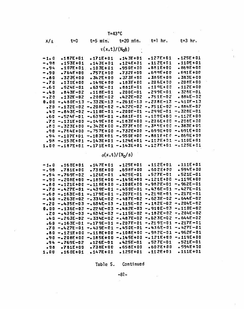
T=43°C xl! t=O t=5 min". t=20 min. t=l hr. t=3 hr.

T(x,t)/(N043)

-1.0 .187E+Ol .171E+Ol .143£+01 .127E+01 • 125E+Ol -.98 .153£+01 .143£+01 .124E+01 .112£+01 .110£+01 -.94 .107E+U1 .103E+01 .950£+00 .881E+00 .869E+00 -.90 .764E'+00 .757E+OO .732£+00 .6~q£+OO .691E+00 -.80 .323£+00 .342£+00 .373E+00 .385£+00 .383E+00 -.70 .131£+00 .149E+ 00 .183f+OO .206E+00 .208£+00 -.60 .524£-01 • 639E-0 1 .S61£-01 .10QE+OQ .112E+00 -.40 .843£-02 .118E-01 .200E-Ol .299E-01 .328£-01 -.20 .132E-02 .208E-02 .422E-02 .751E-02 .884£-02 0.00 -.480£-13 -.332E-13 -.261E-13 -.238E-13 -.410F-13

.20 -.132E-02 -.206E-02 -.422E-02 -.751E-02 -.884£-02

.40 -.843E-02 -.118E-01 -.200£-01 -.299E-01 -.328E-Ol

.60 -.524£-01 -.639£-01 -.881£-01 -.10C?£+OO -.112E+00

.70 -.131£+OU -.149E+00 -.163£+00 -.206E+00 -.208£+00

.e 0 -.323E+00 -.342E+00 -.373f+00 -.3P~E+OC -.383E+00

.90 -.764E+00 -.757£+00 -.732E+00 -.699E+00 -.691£+00

.94 -.107E+01 -.103E+01 -.950£+00 -.881£+0 r -.869E+00

.9~ -.153E+01 -.143E+Ol -.124£+01 -.112E+Ol -.110E+01 1.00 -.167£+01 -.171E+01 -.143E+01 -.127£+01 -.125E+01

a(X, t)1 (Nol 6)

-1-0 .160E+01 .147E+01 .125£+01 .112£+01 .111E+01 -.98 .781E+00 .73 8E+0 0 .658f+00 .602E+00 .594£+00 -.94 -.769E-02 .126E-Ol .425E-01 .527E-01 .521E-01 -.90 -.208E+00 -.185E+00 -.145E+00 -.121E+OD -.119£+00 -.80 -.121E+00 -. 11 8E + 0 0 -.108 E + 00 -.982£-01 -.962E-01 - .70 -.427E-Ol -.439£-01 -.450E-Ol -.436E-1Jl -.427E-Ol - .60 -.163E-01 -.179E-01 -.207E-01 -.219E-01 -.217E-Ol -.40 -.263E-02 -.334E-02 -.487E-02 -.623E-02 -.644E-02 -.20 -."35E-03 -.634E-03 -.115E-02 -.182E-02 -.204£-02 0.00 -.136E-03 -.224E-03 -.482E-03 -.910E-03 -.110E-02 .20 -.435E-03 -.634E-03 -.115E-02 -.182E-02 -.204E-02 .40 -.263E-02 -.334E-02 -.487E-02 -.&23E-02 -.644E-02 .60 -.163E-01 -.179E-01 -.207£-01 -.219E-Ol -.217E-Ol .70 -.427E-01 -.439E-Ol -.450E-Ol -."36£-01 -.427f-01 .80 -.121E+00 -.118E+00 -.108E+00 -.982E-01 -.962£-01 .90 -.208E+00 -.185E+00 -.145E+00 -.121E+OO -.119E+00 .94 -.769E-02 .126E-0 1 ."25E-Ol • 52 7E-Ol .521E-01 .98 .781E+00 .738E+00 .658E+OO .602E+00 .594E+UD

1.00 .160E+Ol .147E+Ol • 125E'+Ol .112E+01 • l11E+Ol

Table 5. Continued

-81-

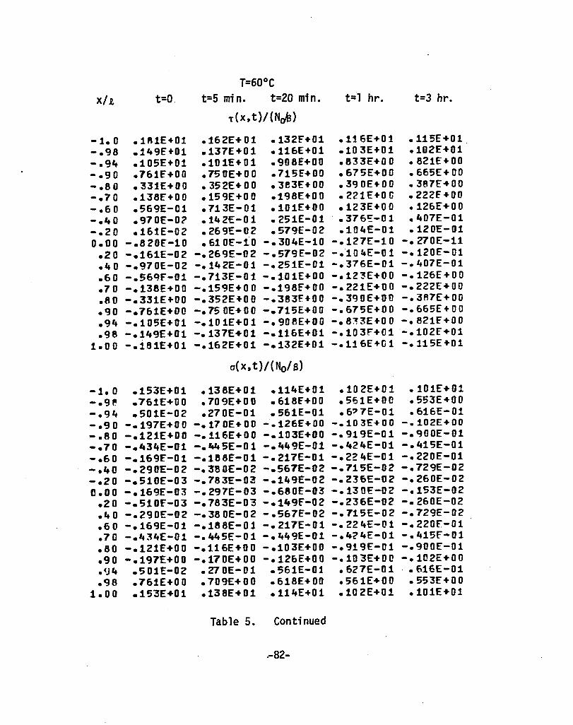
T=60°C x/t t=O, t=5 rni n. t=20 min. t=l hr. t=3 hr.

T(x,t)/(NdB>

-1.0 .1R1E+01 .162E+01 .132F+01 .116E+01 • 115E+Ol -.98 .149E'+01 .137E+01 .116E+01 .103E+Ol .102£+01 -.91t .105£+01 .101£+01 .908E+00 .833£+00 .821£+00 -.90 .761E'+00 .750E+00 .715E+OO .675E+00 .665E+00 -.80 .331E+01) • 352E+ DO • 383E+ 00 .390E+OO .387E+00 -.70 .138£'+00 .159E+00 .198E+OO .221£+0(; .222F+00 -.60 .569E-D1 .713E-01 .101E+00 .123E+00 • 126E+OO -.1t0 .970E-0? .142£-01 .251E-Ol .• 376S::-0 1 .407E-Ol -.20 .161E-02 .269£-02 .579E-02 .104E-01 .120E-01 0.00 -.820E-I0 .610E-io -.304E-10 -.127E-10 -.270E-11 .20 -.161E-02 -.269£-02 - .579E-02 -.10"E-01 -.120£-01 .40 -.970E-02 -.142E-01 -.Z51E-01 -.376E-01 -.407E-01 .60 -.56QF-01 -.713E-01 -.101E+00 -.123£+00 -.126E+0 0 .70 -.138E+00 -.159E+00 -.198F+00 -.221E+DO -.222£+00 .80 -.331E+00 -.352E+00 -.383F+00 -.390E+00 -.3A7£+00 .90 -.761£+00 -.750E+00 -.715E+00 -.675E+OO -.665E+00 .94 -.105£+01 -.10 lE+O 1 -.908E+00 -.8~3E+00 -.821f+00 .98 -.149£+01 -.137E+Ol -.116E+01 -.103F+C1 -.102(+01

1.00 -.181E+01 -.162E+01 -.132E+Ol -.116£+(;1 -.115£+01

a(X, t)/(No/s)

-1.0 .153E+Ol .138E+Ol .114E+Ol .102E+01 .101E+01 -.9P. .761£+00 .709E+00 • 618F+0 0 .561E+00 .553£+00 -.94 .501E-02 .270E-01 .561E-01 • 6:;J 7E-01 .616E-01 -.90 -.197E+00 -.170E+00 -.126£+00 -.103E+00 -.102E+00 -.80 -.121E+00 -.116E+00 -.lD3E+00 -.919E-01 -.900E-01 -.70 -."34E-Ol - ..... 5E-Ol -.449E-01 -.424E-01 -.415E-01 -.60 -.169£-01 -.188E-01 -.217E-01 -.224E-Ol -.220E-Ol -.40 -.290£-02 -.3S0E-02 -.567E-02 -.715E-02 -.729E-02 -.20 -.510E-03 -.783£-03 -.149E-02 -.236£-02 -.260E-02 0.00 - .169E-03 -.297E-03 -.6S0E-03 -.130£-02 -.153E-02

.20 -.510r-03 -.783E-03 -.149F-02 -.236E-02 -.260E-02

... 0 -.290£-02 -.380E-02 -.567E'-02 -.715E-02 -.729£-02

.60 -.169£-01 -.188E-01 -.217E-01 -.224£-01 -.220F.-Ol

.70 -.434E-Ol -.445E-01 -.Zt49E-01 -.424£-01 -.415F-Ol

.80 -.121E+00 -.116E+00 -.103E+00 -.919£-01 -.900E-01

.90 -.197E+00 -.170E+00 -.126E+OO -.1D3E+OC -.102E+OO

.94 .501E-02 .270E-01 .561E-01 .627E-01 .616E-01

.98 .761E+00 .709E+00 .618E+00 .561£+00 .553f+00 1.00 .153E+01 .138E+01 .114E+01 .102E+01 .101E+01

Table 5. Continued

.-82-

T=82°C xlR. t=O t=5 min. t=20 min. t=l hr. t=3 hr.

' ..

T(x,t)/(N~)

-1.0 .176E+01 .155E+Ol .123E+01 .108E+Ol .107E+01 -.98 .146E+01 .132E+01 .109E+01 .971E+00 • 958E+0 0 -.94 .104E+01 .984E+00 .874E+00 .795E+00 .783E+00 -.90 .758E+00 .74"3£+00 .699E+00 .653E+00 .643E+00 - .80 .337£+00 .360E+00 .391£+00 .393E+00 .389£+00 -.70 .143E+00 .168£+00 .210E+00 .231E+00 .231£+00 - .60 .604f-01 .775E-01 .111E+00 .135E+00 .137[+00 -.40 .107E-Ol .163E-Ol .299[-01 .444E-Ol .474£'-01 -.20 .184E-02 .326E-02 .732E-02 .131E-Ol .14Af"-Ol 0.00 -.220E-10 -.208E-11 -.733f-13 .177E-14 -.~qR£,-13

.20 -.184E-02 -.326E-02 -.732E-02 -.131E-Ol -.148E-Ol

.40 -.107E-01 -.163E-Ol -.299£-01 -. 44"E-0 1 -.474f-Ol

.60 -.604F-Ol -.775[-01 -.111f+00 -.135E+00 -.137£+00

.70 -.143£+00 -.168E+00 -.210E+00 -.231£+00 -.231£'+00

.80 -.337E+00 -.360£+00 -.391E+00 -.393E+00 -. ~89F+0 0

.90 -.758E+00 -.743£+00 -.699E+00 -.653E+00 -.643E+00 • CPt -.104[+01 -.984E+00 -.874£+00 -.7~5E+OD -.783E+00 .98 -.146E+01 -.132E+01 -.109£+01 -.971[+00 -.958E+00

1.00 -.176£'+01 -.155E+01 -.123E+01 -.108~+01 -.107E+01

a(x,t)/(No/s)

-1.0 .1'+5E+Ol .128E+Ol .104E+01 .921E+00 .910E+00 -.98 .741£+00 .682E+00 .582f+00 .524E+00 • 517E+ 00 -.94 .212£-01 .445E-01 .718f-Ol • 7ft 7E-0 1 .733E-01 -.90 -.185E+00 -.154E+00 -.107£+00 -.865E-Ol -.854E-Ol -.80 -.121£+00 -.115E+00 -.100E'+OO -.879E-Ol -.861E-01 -.70 -."42£-01 -.453E-01 -."50E-Ol -. 417E-0 1 -.407E-Ol -.60 -.174£-01 -.195E-01 -.224E-Ol -.226E-01 -.221E-Ol -.It 0 -.311E-02 -.418E-02 -.63'+E-02 -.785E-02 -.792£-02 -.20 -.570E-03 -.916E-03 -.181£'-02 -.285E-02 -.308E-02 0.00 -.196£-03 -.365E-03 -.878E'-03 -.167£-02 -.193£-02

.20 -.570E-03 -.916E-03 -.181E-02 -.265E-02 -.308E-02

.40 -.311E-02 -.418E-02 -.634E-02 -.785E-02 -.792£-02

.60 -.17.4£-01 -.195E-Ol -.224£-01 -.226E-01 -.221E-Ol

.70 -.442E-01 -.453E-01 -.,,50E-Ol -.417E-01 -.407£-01

.80 -.121E+00 -.115E+00 -.100E+00 -.879E-01 -.861£-01

.90 -.185E+00 -.154E+00 -.107E+00 -.865E-01 -.854£-01

.94 .212£-01 .445E-01 .718E-01 .74 7E-0 1 .733£'-01 .91\ .741£'+00 .682E+00 .582E+00 • 524E+0 0 .517E+00

1.00 .145f+01 .128E+01 .104£'+01 .921E+00 .910E+00

Table 5. Continued

-83~

T=2l0C

x/I. t=O t=5 min. t=20 min. t=l hr. t=3 hr.

T{X,t)/(Qo/S)

-1.0 -.140E+03 -.129E+ 03 -.110£+03 -.980E+02 -.964E+02 -.98 -.116E+03 -.109E+03 -.957E+02 -.865E+02 -.851E+02 -.94 -.830E+02 -.799E+02 -.737E+02 -.684E+02 -.673E+02 -.90 -.589E+02 -.580E+02 -.559[+02 -.532E+0? -.525E+02 -.80 -.199£+02 -.213E+02 -.236F+02 -.246E+02 -.245E+02

.. -.70 -.247£+01 -.380£+01 -.639[+01 -.829£+01· -.852[+01 -.60 .448£+01 .364£+01 .183(+01 .1130£+00 -.12~E+OO -.it 0 .826£+01 .803£+01 .744E+01 .672E+01 .649E+01 -.20 .884F+01 • 879E+0 1 .864F+01 .8ltOE+01 .828E+01 0.00 .893£+01 .892£+01 .889E+01 .881E+01 .877£+01

.20 .895[+01 .891t£+01 .89ltE+Ol .892F+D1 • 891l[foOl

.40 .695£+01 .895£+01 .895E+01 .895E+n1 .694£+ 01

.60 .897E+01 .897[+01 .898E+Ol .897E+01 .897£+01

.70 .901£+01 .901E+01 .901£+01 .900E+01 .900F+01

.80 .910E+01 • 909E+0 1 .907f+01 .905E+01 .904£+01

.90 .903£+01 .901£+01 • 897E+Ol .8135£+01 .695[+01

.94 .875£+01 .675E+01 .876f+Ol .877E+01 .877f+01

.98 ."31E+01 • 836E+0 1 • e46F+01 .852E+01 .853£+01 1.00 .819£+01 .826E+01 .838£+01 .846£+01 .847£+01

a(x,t)/(Qo/a)

-1.0 -.207£+03 -.195E+03 -.174E+03 -.162E+03 -.161E+03 -.98 -.879£+02 -.847E+02 -.787[+02 -.7lt2E+02 -.735£+02 -.94 .120£"02 .999E+01 .683F+Ol .543E+U1 .542£+01 -.90 .295E+02 .278E+02 ~ 246E+02 .226£+02 .224E+02 -.80 .124£+02 .122F+02 .1.16£+02 .1.09E+02 .108E+02 -.70 .384E+01 .392E+Ol .399£+01 .390E+Ol .384F+01 -.60 .142£"'01 .15"E+01 .175E+01 .186E+01 .185F+D1 . -.40 • 221E+00 • Z7~E+OO .386E+00 .493£+00 .511E+00 -.20 .3"OE-01 .474E-01 .812£-01 .125£+00 .139E+00 0.00 .526£-02 .820£-02 .167E-01 .309E-01 .376E-Ol

.ZO .986E-03 .163E-02 .369£-02 .7'i6E-02 .105£-01 " .40 .130E-02 .155E-02 .220E-02 .33"'£-02 .426E-02

.60 .700F.-02 .664£-02 .566E-02 .461t£-02 • "68E-O? .70 .'301£-01 • 302£- 01 .301E-01 .300E-01 .302F-01 .80 .203E+00 .213E+00 .231[+00 .2'+3E"00. • 245£+00 .90 .259E+OO .240E+00 .205£+00 .IR5E+00 • 184E+00 .94 -.136E+01 -.143E+Ol -.154E+Ol -.160£+01 -.161E+Ol .98 -.753E+01 -.751E+Ol -.747E+Ol -.744E+01 -.7"4£+01

1.00 -.142E+02 -.139E+02 -.135£+02 -.132E+02 -.132£+02

Table 6. Adhesive stresses for a cover plate subjected to trans-verse shear loading (QofO, No=Mo=6T=O) for T=21oC, 43°C, 60°C, and 82°C, where hl=.762rnm, h2=2.286rnm, ho=·1016rnm, 1.=12.7rnm, and S=2.54xlO-2m.

-84 ..

T=43°C x/R. t=O t=5 min. t=20 min. t=l hr. t=3 hr.

T(X, t)1 (Qol s)

-1.0 -.136£+03 -.12"E+03 -.104£+03 -.918E+02 -.904E+02 -.98 -.113E+03 -.105E+03 -.911£+02 -.817£+02 -.804E+02 -.94 -.819E+02 -.783E+02 -.712E+02 -.655E+02 -.644£+02 -.90 -.586£+02 -.575E+02 -.548£+02 -. 517E+0 2 -.509£+02 -.80 -.204E+02 -. 219E+ 02 -.243£+02 -.251E+02 -.249£+02 -.70 -.294E+01 -.4It6E+01 -.132£+01 -.925E+01 -.941E+Ol - .• 60 .419~+01 .319E+Ol .111f+01 -.68UE+DO -.973£+00 -.40 .818E+01 • 789E+ 01 .716E+01 .630£+01 .604E+01 -.20 .882£+01 .875E+01 .855E+01 .824E+01 .810E+01 0.00 .893E+01 .891E+Ol .886E+Ol .876E+01 .870E+Ol

.20 .895E+01 • 89ltE+ 0 1 .693E+01 .890E+01 .888E+01

.40 .895£+01 .895£+01 .895E+01 .89ltE+01 .893£+01

.60 .897£+01 .897E+Ol .898£+01 .e~7E+01 .897F+01

.70 .901E+01 .901£+01 .901£+01 .9r.JOE+Ol .900E+01

.80 .909£+01 .908E+Ol .9061:+01 .90 4E+0 1 .904E+01

.90 .902E+01 .900E+Dl • ~96E+Ol .894E+01 • 894E +01

.94 .875E+01 • 875E+0 1 .876E+Ol • ~77E+01 .878f+01

.98 .832E+01 • 838E+0 1 .848E+01 .855E+01 .856f+Ol 1.00 .821E+01 .828E+Ol .841E'+01 .850E+01 .851£+01

a(x,t)/(Qo/s)

-1.0 -.201E+03 -.187£+03 -.166E+03 -.154E+03 -.152£+03 -.98 -.866E+02 -.829E+02 -.762E+02 -.715E+02 -.708£+02 -.94 .107E+02 .862E+01 .542£+01 .422E+Ol .lt25E+Ol -.90 .287E+02 .267E+02 .233£+02 .213E+02 .211E+D2 -.80 .124£+02 .121E+02 .114£+02 .106£+02 .105£+02 -.70 .388E+01 .396E+Ol • '40 OE+O 1 .385£+01 .378£+01 -.60 .146E+Ol .159E+Ol .181E+Ol .190£+01 .188£+01 -.It 0 .238E+00 .300E+00 .433E+00 .5'+8E+00 .564E+00 -.20 .384E-Ol .553E-01 .978F-Ol .151E+OO .165£+00 0.00 .622£-02 .101E-01 .216E-01 .404E-Ol .486E-Ol

.20 .120£-02 .209£-02 .502£-02 .110E-01 .146£-01

.40 .140E-02 .172E-0 2 .260£-02 .430E-02 .567E-0"2

.60 .699£-02 .6r;2E-02 .529E-02 .42 f-E-O 2 .452£-02

.70 .311£-01 .313E-01 .314E-01 .317E-Ol .321E-01

.80 .211E+OO • 222E+0 0 .243E+00 • 256E+0 0 .257E+00

.9D .239E+00 .216E+00 .177f+OO .156E+1)0 .154E+OO

.94 -.141E+01 -.149E+Ol - .161E+01 -.167£+01 -.167E+01

.98 -.751E+01 -.748E+01 -.743£+01 -.7'+1E+D1 -.740E+Ol 1.00 -.140E+02 -.137E+02 -.132E+02 -.13UE+1l2 -.130E+02

Table 6. Continued

-85-

T=60°C xl! t=O t=5 min. t=20 min. t=l hr. t=3 hr.

T(x,t)/(Qo/s)

-1.0 -.131E+0'3 -.118E+03 -.C355E+02 -.~37E""02 -.824E+02 -.98 -.11 OE+O 3 -.101E+03 -.849£+02 -.753f+02 -.741£+02

-.9" -.80,.£+02 -.761£+02 -.677E+02 -.61"E+02 -.604E+02 -.90 -.582E+02 -.567£+D2 -.531F+02 -.,.9,.E+02 -.486£+02 -.80 -.211E+02 -.227E+02 -.250E+02 -.25"E+02 -.251E+02 -.70 -.355E+Ol -.537E+Ol -.861£+01 -.105£+02 -.105F+02 -.60 .380E+01 • 255E+0 1 .34C3E-01 -.191E+Ol -.215£+01 -.40 .807£+01 • 7E 7E+Ol .671E+01 .561E+Ol .534£+01 -.20 .880£+01 .870E+Ol .840E+Ol .7CJ5E+Dl .777f+Ol 0.00 .892E+01 .890£+01 .882£+01 .666£+01 .857[+01

.20 .894£+01 .89 .. E+01 .892E+01 .867E+01 • e83E+ 01

.40 .895E+01 • 6C35E+ 0 1 • 895E+ 01 .89'3E+Q1 .892E+01

.60 .e97E+01 .898£+01 .898£+01 .897E+Cl .896F+01 .70 .c}01E+01 .901£+01 .901E+01 .900E+01 .899£+01 .80 .909E+Ol .908E+01 .905E+01 .90 "3E+O 1 .902E+Ol .90 .C}01E+01 .898E+Ol .89,.[+01 .893E+C1 .893[+01 .94 .874E+01 .87,.£+01 .876E+01 .878£+01 .87BE+01 .98 .833[+01 • A4 DE+ 0 1 .852£+01 .85C3E+01 .860[+01

1.00 .823£+01 .831E+01 .846£+01 .855[+01 .855E+01

a(x,t}/(Qo/s}

-1.0 -.193[+03 -. 17 8E+O~ -.154[+03 -.143E+03 -.142E+03 -.98 -.848[+02 -.805E+02 -.728E+02 -.67c}E+D? -.672E+02 -.94 .924£+01 '.68 9E+0 1 .369F+Ol .282E+01 .290£+01 -.90 .277E+02 .25"E+02 • 216£+02 .197E+02 • 196E+02 -.80 .124E+02 .12 OE+O 2 .111E+02 .102£+02 .101E+02 -.70 .393E+Ol .400E+01 .398E+01 .374E+01 • 366E+01 -.60 .151E+Ol .167[+01 .189[+01 .193E+Ol .189E+01 -.40 .262£+00 .3"1£+00 .501E+00 .624[+00 • 633E+00 -.20 .448£-01 .677E-Ol .125£+00 .191£+00 .206F+00 0.00 .768£-02 .13,.E-01 .303E-01 .572E-01 .673E-01

.20 .153E-02 .29 OE-O 2 .757£-02 .171£-01 .2?3E-01

.40 .155£-02 .200E-02 .335E-02 .630E-02 .858£-02

.60 .694£-02 .628E-02 .472£-02 .392£-02 .468F.-02

.70 .326£-01 .330E-Ol ."336£-01 .3,.5E-01 .352E-01

.80 .221E+00 .235£+00 .259E+00 .272E+00 • 27,.F +0 0

.9tJ .213E+00 .184E+ 00 .137E+00 .116E+00 .115£+00

.9,. -.1"8E+01 -.157E+01 -.170£+01 -.175E+C1 -.1i"5E+01

.98 -.748E+01 -.744E+01 -.738E+01 -.735E+01 -.735E+01 1.00 -.137E+02 -.134E+02 -.128E+02 -.126E+02 -.126E+02

Table 6. Continued

-86-

T=82°C xl! t=O t=5 min. t=20 min. t=l hr. t=3 hr.

.r( x, t)/(Qo/s)

-1.0 -.128E+03 -.112E+ 03 -.890E+02 -.775E+02 -.76"£+02 -.98 -.108£+03 -.971E+02 -.799[+02 -.70lE+U2 -.692£+02 -.9" -.792E+02 -.7"1£+02 -.6"7E+02 -.5~1E+02 -.571£+02 -.90 -.578E+02 -.560£+02 -.516£+02 -. "7'+£+02 -.'+66[+02 -.80 -.216£+02 -.23"E+02 -.256£+02 -.256E+02 -.252F.+02 -.70 -.403£+01 -. 612E+0 1 -.964£+01 -.114E+02 -.113£+02 -.6 ('! .350£+01 .202E+01 -.P.63E'+00 -.287E+01 -.305£+01 -."0 .798£+01 .749£+01 .629E'+01 .501E+01 • "73£+01 -.20 .878£+01 • 86ltE+ 01 .826E+Ol .767£+01 .• 7'+7E+Ol 0.00 .892E'+01 .889E+Ol .877E+01 .855E+01 .843£+01

.20 .894['+01 .894£+01 .891E+01 .8J\'3E+01 .877[,+01

.It 0 .895E+01 .895£+01 .895£+01 .892E+01 .889E+01

.60 .898F+01 • 8~8E+0 1 .898£"+01 .897E+01 .895E+01

.70 .902£+01 .90 2E+0 1 .901£+01 .899£+01 .898£+01

.80 .910E+01 .908£+01 .905F+01 .902E+Ol .901E'+01

.90 .900E+Ol .897£+01 .893E+Ol .892£+01 .892£+01

.94 .873£+01 • 873E+0 1 .875£+01 .878£+01 .878E+01

.98 .833£+01 .841E+01 .854E+Ol .851E+01 .861[·01 1.00 .823£+01 .832E+01 .8"9£+01 .857E+01 .857£+01

a(x,t)/{Qo/s)

-1.0 -.183£+03 -.166£+03 -.142£+03 -.131£+03 -.130F.+03 -.98 -.829E'+02 -.778E+02 -.693E+02 -.6'+3£+02 -.637£+02 -.9 .. .713£+01 • '+56E+01 .1'+1E+01 • 8'+9E+0 0 .957£+00 -.90 .264£+02 .238£+02 .197[+02 .179£+02 .178£+02 -.80 .126E+02 .121E+02 .110£+02 .101E+02 .993£+01 -.70 ."01£+01 • ,,07E+01 .399£+01 .369E+01 .360£+01 -.60 .155£+01 .172£+01 .193E+Ol .192E+01 .188E+Ol -.40 .280£+00 .37'+E+OO .558£+00 .681£+00 .684[+00 -.20 ."99£-01 .787E-01 .150£+00 .227£+00 .241f+00 0.00 .889£-02 .164E-Ol .391£-01 .736E-01 .8'+7F-01

.20 .182£-02 .372E-02 .103£-01 .237E-01 .302£-01

.40 .171E-02 .232E-02 .424E'-02 .870E-02 .119E-ol

.60 .713E-02 • 629E-0 2 .445E'-02 .409C::-02 .540f-02

.70 .363E-Ol .375E-Ol .397E-01 .419E-Ol .431£-01

.80 .237£+00 • 255E+0 0 .283f+00 .298E+{l0 • 299E'+00

.90 .162£+00 .122E+00 .609£-01 .364£-01 .359E-01

.94 -.159E~01 -.1£.9£+01 -.183E'+01 -.188£+01 -.188£+01

.98 -.7'+1[+01 -.736E+Ol -.728E+Ol -.725E+01 -.725£+01 1.00 -.13"3E'+02 -.12 8E+0 2 -.123£+02 -.121£+02 -.121E+02

Table 6. Continued

-87-

T=2l0C xlR, t=O t=5 min. t=20 min. t=l hr. t=3 hr.

T(x,t)/(6T/s)

-1.0 .344E+0~ .317E+02 .271E+02 .2,.1E+02 .238E+02 -.98 .279E+02 .263E+0~ .232£+02 .210E+02 .207£+02 -.94 .193E+02 .187E+02 .174£+02 .16'3£+02 .161£+02 -.90 .137£+02 .136£+02 .133£+02 .128E+02 .126£+02 -.80 .565E+01 .596£+01 .649E+01 .675E+(,1 .674E'+01 - .70 .22,.E+01 .252£+01 .306£+01 • 3,.7E+·0 1 .352E+01 -.60 .876E+00 .105E+01 .142E+01 .176E+01 .183£+01 -.40 .135£+00 .182E+00 .300E+00 • 446E+0 0 .4r:t3F+OO -.20 .202£-01 .306£-01 .595£-01 .105E+00 .124£+00 0.00 .<375E-11 -.1"3E-10 -.478E-11 -.215£-11 -.187£:-11

.20 -.202E-01 -.306~-01 -.595£-01 -.105E+OC -.124E'+OO

.40 -.135£+00 -.182E+00 -.300E+00 -.4,.6£+0(1 -.49!E+OO

.60 -.876£+00 -.1D5E~01 -.142£+01 -.176£+01 -.18!f+01

.70 -.224E+01 -.2~2£+01 -.306£+01 -.347E+01 -.352E+01

.80 -.565£+01 -.596E+01 -.649E+01 -.675E+01 -.674E+01

.90 -.137E+02 -.136E+02 -.133[+02 -.128£+02 -.126£+02

.94 -.193£+02 -.187E+02 -.17"£+02 -.163f+02 -.161E+02

.98 -.279£+02 -.263E+02 -.232£+02 -.21DE+0~ -.207E+02 1.00 -.344£+02 -.317E+02 -.271[+02 -.241£+02 -.238E+02

a(x, t)/(6T/s)

-1.0 .296E+02 • 274E+0 2 .237£+02 .214f'+02 .211£+02 -.98 .142E+02 .135E+02 .122E+02 .113£+02 .111£+02 -.94 -.325f+00 .166E-0 1 .552£+00 • 776E+0 0 .773£+00 -.90 -.388£+01 -.351£+01 -.284E+01 -.241£+01 -.236E+01 -.80 -.218£+01 -.212E+01 -.198£+01 -.183£+01 -.179E+01 -.70 -.753E+00 -.774£+00 -.799£+00 -.786£+00 -.773E+00 -.60 -.281£+00 -.308£+00 -.355£+00 -.'381E+00 -.379E+00 -.40 -.434E-01 -.540E-01 -.773E-01 -.996£-01 -.104£+00 -.20 -.684£-02 -.964E-02 -.169£-01 -.266E-D1 -.300E-01 0.0'0 -.206E-02 -.323E-02 -.665£-02 -.124E-D1 -.151E-01 .20 -.684E-02 -.964E-02 -.169£-01 -.266E-D1 -.300E-01 .,. 0 -.434E-01 -.540E-01 -.773E-01 -.9g6E-01 -.104£+00 .60 -.281E+00 -.308£+00 -.355£+00 -. ~~ 1£+0 0 -.379£+00 .70 -.753E+00 -.774E+00 -.799£+00 -.7~6E+DO -.773£+00 .80 -.218E+01 -.212£+01 -.198£+01 -.183E+01 -.179E+Oi .90 -.38AE+01 -.351E+01 -.284E+01 -.2,.1 £+D1 -.236E+01 .9,. -.325E+00 .166E-01 .552E+00 • 776E+0 0 .773E+OO .98 .142E+02 • 135E+02 .122£+02 .113E+02 .111E+02

1.00 .296E+02 • 274E+ 02 .237£+02 .214E+02 .211E'+02

Table 7. Adhesive stresses for. a cover plate resulting from a temperature increase (6T~O, No=Mo=Qo=O) for T~=2loC, 43°C, 60°C, and 82°C, where hl=.762mm h7=2.2 6mm, ho= .1016mm, R,=12.7mm, and S=(2.54xlO-2m)~(5 gOC)/(4.448N).

-88-

T=43°C x/R. t=O t=5 min. t=20 min. t=l hr. t=3 hr.

'rex, t)/(l1T/S)

-1.0 .334E+02 .305E+02 .256£+02 .221E+02 .223E+02 -.98 .213E+02 • 255E+0 2 .221[+02 .199E+02 .197£+02 -.9ft .191E+02 .184E+02 .169E+02 .151E+02 .155E+02 -.90 .136£+02 .135E+02 .131[+02 .125£+02 .123£+02 -.80 .516£+01 .61 OE+ 0 1 .665[+01 .6e6E+C1 .683E+01 -.70 .233E+01 • 265E+0 1 .326["'01 .367E+01 .371E+01 -.60 .936E+00 .114E+Ol .157[+01 .1~5E+Ol .201E+01 -.4 C .151E+00 .21 OE+ 0 0 .356E+00 • 5~3£+0 0 .585E+DC -.20 • 236E-0 1 .371~-01 .754£-01 .134£+00 .158E+00 0.00 -.e56E-12 -.593E-12 -.466E-12 -.425E-12 -.131E-12

.20 -.236E-01 -.371£-01 -.754£'-01 -.13ItE+00 -.158E+00

.40 -.151E+00 -.210£+ 00 -.356E+00 -.533E+00 -.585E+OC

.60 -.C;\36£+00 -.114£+01 -.157[+01 -.195[+01 -.201£+01

.70 -.233E+01 -. 265E+0 1 -.326[+01 -.367E+01 -.371£+01

.80 -.516£+01 -.610E+Ol -.665E+01 -.6~6f+01 -.6A3E+01

.90 -.136E+02 -.135E+02 -.131E'+D2 -.12S;;~+(l2 -.123E+02

.94 -.191£+02 -.184E+02 -.169[+02 -.157E+02 -.155£+02

.98 -.273E+02 -.255E+02 -.221£+02 -.199E+02 -.197E+02 1.00 -.334E+02 -.30 5E+0 2 -.256E+02 -. 22 7~+02 -.223E+02

a(x,t)/(l1T/S)

-1.0 .285E+02 • 262E+ 02 .222E+02 .200E+O? .197[+02 -.98 .139E+02 .132E+02 .117E+02 .101E+02 • 106[+02 -.94 -.131E+OO .225£+00 .758F+OO .940E+00 .92c;\£+00 -.90 -.372£+01 -. 330E+ 01 -.259E+01 -.216£+01 -.212E+Ol -.80 -.217[+01 -.210£+01 -.193£'+01 -.175£+01 -.172E+01 -.70 -.763E+OO -.784E+00 -.802E+00 -.777E+00 -.763E+00 - .60 -.290E+00 -.320E+OO -.370£+00 -.391E+00 -.387[+00 -.40 -."70E-01 -.596£-01 -.869£-01 -.111E+0[! -.115£+00 -.20 -.776E-02 -.113£-01 -.205E-Ol -.325£-01 -.363£-01 0.00 -.243[-02 -.399E-02 -.861E-02 -.162E-01 -.196E-01

.20 -.776[-02 -.113[-01 -.205[-01 -.325E-01·-.363E-01

.40 -.470E-01 -.596£-01 -.869£-01 -.111£+00 -.115E+OO

.60 -. 290E+ 00 -.320£+00 -.370E+00 -.391E+OC -.387E+00

.70 -.763£+00 -.784E+00 -.802£+00 -.717E+00-.763[+00

.80 -.217£+01 -.210E+01 -.193[+01 -.175E+01 -.172E+01

.90 -.372[+01 -.330E+01 -.259E+01 -.216E+01 -.212E+01

.94 -.137£+00 c 225E+OO .756E+OO .94DE+OO .929E+00

.98 .139E+02 .132E+02 .117E+02 .107E+02 .106E+02 1.00 .285[+02 .262E+02 .222E+02 .200E+02 .197£+02

Table 7. Conti nued

-89- .'

T=60°C

xh. t=O t=5 min. t=20 min. t=l hr~ t=j hr.

·rex, t)/(AT/S)

-1.0 .323£+02 .289E+02 .235E+02 .207E+02 .204E'+02 -.98 .266£+02 .244E+02 .207£+02 .185E+02 .182E+02 -.94 .188£+02 • 179E+ 02 .162£+02 .1"~E+02 • 147E+02 -.90 .136£+02 .134£+02 .128£'+02 .120E+02 .119£+02 -.RO .590E+01 • 628E+0 1 .684E+01 .697E+Ol .691E+01 -.70 .246E+01 • 284E+0 1 .353E-'01 .394E+01 .395£+01 -.60 .102E+Ol .127E+01 .179E+Ol .220E+01 .225E+01 - .40 .173E+00 • 253E+ 00 .449f+00 .672E+00 .72E,E+OO -.20 .287E-Ol .48 OE-01 .103£+00 .1~5E+OO .214E+00 0.00 -.146E-08 .109£-08 -.542E-09 -.226E-09 -.482E-10

.20 -.287£-01 -.480E-Ot -.103£+00 -.1"5E+(l0 -.214£'+00

.40 -.173E+OO -.253E+00 -."49E+00 -.672£+0(1 -. 7Z~E+OO

.60 -.102£+01 -.127E+01 -.179E+01 -.220E+lH -.225£+01

.70 -.246£+01 -.21' 4E+0 1 -.353E'+01 -.39 4E+0 1 -. 395E +01

.80 -.590f+Ol -.628E+01 -.684£+01 -.697£+U1 -.691£+01

.90 -.136E+02 -.134E+02 -.128f+02 -.120E+02 -.119f+02

.94 -.188E+02 -.179E+02 -.162£+02 -.149E+02 -.147£+02

.98 -.266F+02 -.244£+02 -.207£+02 -.185E+02 -.182£+02 1.00 -.323E+02 -.289E+02 -.235E+02 -.207E+02 -.204[+02

a(x,t)/(AT/S)

-1.0 .273£+02 • 246E+ 02 .204E+02 .182E+02 • 180F.+02 -.98 .136£+02 .127E+02 .110£+02 .100E+02 .987E+01 -.94 .894£-01 • 483E+0 0 .100f+01 .112E+01 .110E+01 -.90 -.352£+01 -.303E+01 -.225£+01 -.185E+01 -.182F+Ol -.80 -.216£+01 -.206E+Ol -.184£+01 -.164E+Ol -.161£+01 -.70 -.775E+00 -.795£+00 -.801£+00 -.757E+00 -.741£+00 -.60 -.302E+00 -.336E+00 -.388f+00 -.400 E+O 0 -.393E+00 -.40 -.518E-01 -.679£-01 -.101E+00 -.128E+00 -.130E+00 -.20 -.910E-02 -.140E-Ol -.266£-01 -.422E-01 -."64£-01 0.00 -.301E-02 -.529E-02 -.121£-01 -.231E-Ol -.273f-Ol

.20 -.910E-02 -.140£-01 -.266£-01 -.422E-01 -. "64E-01

.40 -.518£-01 -.679E-Ol -.101E+00 -.128E+UO -.130E+00

.60 -.302£+00 -.336E+00 -.388E+00 -.400E+00 -.39~E+OO

.70 -.775£+00 -.795E+00 -.801£+00 -.757E+00 -.741£+00

.80 -.216£+01 -.206E+01 -.184£+01 -.164E+Ol -.161E+Ol

.90 -.352E+Ol -.303E+01 -.225E+01 -.185E+Ol -.182E+01

.94 • 894E-01 .48 3E+0 0 .100f+01 .112£+01 . .110E+01

.98 .136E+02 .127E+02 .110£+02 .100E+02 • 987E+ 01 1.00 .273E'+02 .246E+02 .204E+02 .162E+02 .180E+02

Table 7. Continued

-90-

T=82°C x/R. t=O t=5 min. t=20 min. t=l hr. t=3 hr.

T(X,t)/(6T/S)

-1.0 .315E+02 .277E+02 .220E+02 .193E+02 .190E+02 -.98 .260£+02 .236£+02 .195£+02 .173E+02 .171E+02 -.94 .186E+02 .176E+02 .156E+02 .142£+02 .140E+02 -.90 .135E+02 .133£+02 .125E+02 .117E+02 .115E+02 -.80 .6 01E +01 • 643E+0 1 .697E+01 .701E+01 .694E+01 -.70 .256E+01 .300Ei-01 .375f+01 .41 '3F+t:l1 .412£+01 -.60 .108£+01 .138E+01 .198E+Ol .240£+01 .244£+01 -.1t0 .191£+00 \..291E+00 .533£+00 .793E+00 .846[+00 -.20 .329£-01 .582E-01 .131E+00 .234£+00 .265£+00 0.00 -.393E-09 -.371£-10 -.131E-11 .316E-13 -.160E-11

.20 -.329£-01 -.582£-01 -.131E+00 -.234£+00 -.265E+00

.4 (! -.191£+00 -.291£+00 -.533E+00 -.793E+O(l -.846E+00

.60 -.108E+01 -.138f+01 -.198£+01 -.24UE+01 -.244£+01

.70 -.256E+01 -.300E+01 -.375E+Ol -.413E+Ol -.412E+01

.80 -.601£"+01 -.643£+01 -.697F+Ol -.701£+01 -.694E+Ol

.90 -.135f+02 -.133E+02 -.125E+02 -.117£+02 -.115£+02

.94 -.186£+02 -.176E+02 -.156E+0? -.142E+02 -.140£+02

.98 -.260E+02 -.236£+02 -.195E+02 -.173E+02 -.171E+02 1.00 -.315E+02 -.277E+02 -.220E+02 -.193E+(]2 -.190F+02

a(X,t)/(6T/S)

-1.0 .258£+02 .229E+02 .1P.5£+02 .16~E+02 .162£+02 -.98 .132E+02 .122£+02 .104E+02 .935£+01 .922E+01 -.94 .378E+00 .794E+00 .128E+01 .133E+01 .131E+01 -.90 -.330E+01 -.275£+01 -.191£+01 -.15'+£+01 -.152E+01 -.80 -.217[+01 -.205E+01 -.17C:»E+01 -.157£+01 -.154E+01 -.70 -.789E+00 -.809E+00 -.803E+00 -.74'+E+OO -.726E+OO -.60 -.311£+00 -.346E+00 -.400E+00 -.403E+OO -.394£+00 -.40 -.555£-01 -.747E-01 -.113£+00 -.140£+00 -.1'+lE+00 -.20 -.102£-01 -.164£-01 -.322E-Ol -.50~E-01 -.550£-01 0.00 -.350E-02 -.652E-02 -.157E-01 -.298£-01 -.344E-01

.20 -.102E-01 -.164E-01 -.322£-01 -.508E-01 -.550E-01

.40 -.555E-01 -.747£-01 -.113E+00 -.140E+00 -.141E+OO

.60 -.311E+OO -.3'+6£+00 -.400£+00 -.403£+00 -.394E+OO

.70 -.789E+00 -.809E+00 -.803E+00 -.744E+O(l -.726E+OO

.80 -.217E+01 -.205E+Ol -.179E+01 -.157E+01 -.154E+01

.90 -.330E+01 -.275E+01 -.191E+01 -.154£+01 -.152E+01

.94 .378E+CO .794E+OO .128E+D1 .133E+Ul .131E+01

.98 .132E+02 • 122E+0 2 .104£+02 • 935E+0 1 .922E+01 1.00 .258E+02 .229E+02 .185E+02 .164E+02 .162E+02

Table 7. Continued

-91-

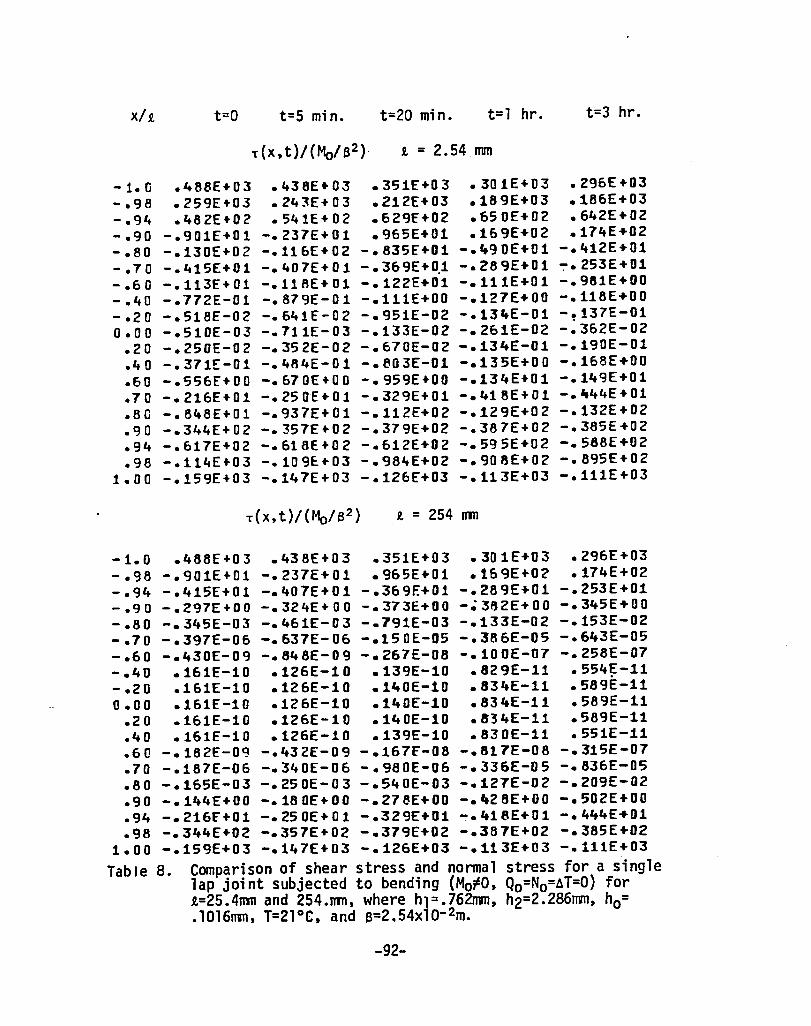
xh.

-1.0 -.98 -.94 -.90 -.80 -.70 -.60 -.40 -.20 0.00

.20

.40

.60

.70

.80

.90

.94

.98 1.00

t=O

.488E+03 .259E+03 .482[+02

-.901E+01 -.130£+02 -.415E+Ol -.113E+01 -.772E-01 -.518E-02 -.510E-03 -.250[-02 -.371[-01 -.556E'+OO -.216E+Ol -.8lt8E+Ol -.344[+02 -.617E+02 -.114E+03 -.159E+03

t=5 min.

.438E+03 • 243E+ 03 • 541E + 02

-.237E+Ol -.116E+02 -.407E+01 -.118E+01 -. 879E-0 1 -.641 E' - 02 -.711E-03 -.352E-02 -.484E-01 -.670£ + 00 -.250E+Ol -.937E+Ol -. 357E+0 2 -.618E+02 -.109E.+03 -.147E+03

t=20 min. t=l hr.

1 = 2.54 mm

.351E+03

.212E+03

.629E'+02

.965E+01 -.835E'+01 -.369E+0.1 -.122E+01 -.111E+00 -.951E-02 -.133E-02 -.670E-02 -. eo 3E-01 -.959E+00 -.329E+01 -.112E+02 -.379[+02 -.612E+02 -.98"'E+02 -.126E+03

.301E+03

.189E+03

.650E+02

.169E+02 -."90E+01 -.289E+01 -.111E+0 1 -.127E+00 -.134E-01 -.261E-02 -.134E-01 -.135E+00 -.134E+Ol -.418E+01 -.129E+02 -.367E+02 -.595E+02 -.908E+02 -.113E+03

1. = 254 rrm

t=3 hr.

• 296E +03 .186E+03 .642E+02 .174E+02

-.412E+Ol ~. 253E+Ol -.981E+00 -.118E+00 -~137E-Ol -.362E-02 -.190E-Ol -.168E+00 -.149E+Ol -."44E+Ol -.132E+02 -.385E+02 -.568E+02 -.895E+02 -.111E+03

-1.0 .488E+03 .438£+03 .351E+03 .301E+03 .296E+03 -.98 -.901E+Ol -.237E+Ol .965E+Ol .169E+02 .174E+02 -.94 -.415E+Ol -.407E+01 -.369F.+Ol -.269£+01 -.253E+01 -.90 -.297E+OO -.324E+00 -.373E+00 -;382E+00 -.345E+00 -.80 -.345E-03 -.461E-03 -.791E-03 -.133E-02 -.153E-02 -.70 -.397[-06 -.637E-06 -.150E-05 -.366E-05 -.643E-05 -.60 -.430E-09 -.648E-09 -.267E-08 -.100E-07 -.258[-07 -.40 .161E-l0 .126E-10 • 13'3E-I0 .82 9E-l1 • 554~-11 -.20 .161E-10 .126E-I0 .140E-10 .834E-l1 .589E-l1 0.00 .161E'-10 .126E-l0 .140E-I0 .834E-l1 .589E-11

.20 .161E-I0 .126E-I0 .140E-I0 .8'34E-l1 .589E-11

.40 .161E-l0 .126E-I0 .139E-l0 .830E-11 .551E-l1

.60 -.182E'-09 -.432E-09 -.167E'-08 -.817E-08 -.315E-07

.70 -.187E-06 -.340E-06 -.980E-06 -.336E-05 -.836E-05

.80 -.165E-03 -.250E-03 -.540E-03 -.127E-02 -.209E-02

.90 -.144[+00 -.180E+00 -.278E+00 -.428E+00 -.502E+00

.94 -.216F+01 -.250E+01 -.329[+01 -.418E+01 -.444E+Ol

.98 -.344E+02 -.357E+02 -.379E+02 -.387E+02 -.385E+02 1.00 -.159E+03 -.147[+03 -.126E+03 -.113E+03 -.111E+03

Table 8. Comparison of shear stress and normal stress for a single lap joint subjected to bending (Mo~O, Qo=No=AT=O) for 1=25.4mm and 254.mm, where hl=.762mm, h2=2.286mm, ho= .1016mm, T=2loC, and S=2.54xlO- 2m.

-92-

xl R. t=O t=5 min. t=20 min. t=l hr. t=3 hr.

a{x,t)/{Mo/B2 ) R. = 25.4 nm

-1.0 -.1"9E+0" -.145E+0" -.l"OE+O" -.137E+04 -.137E+0" -.98 -.523E+Ol -.138E+02 -.285E+02 -.371E+02 -.379E+02 -.94 .106E+03 .108E+03 .111E+03 .114£+03 .11"E+03 -.90 ."88E+02 • 499E+02 .520E+02 .537£+02 .5"OE+02 -.80 .813E+01 .796E+01 .766E+Ol .751E+01 .752E+01 -.70 • 176E+Ol" .168£+01 .151E+O'1 .133E+01 .130E+01 -.60 ."31£+00 ."16E+00 • 37 5E+00 .316£+00 .296E+00 -." 0 .282E-01 • 292E-0 1 .306E-Ol .290E-01 .262E-01 -.20 .188£-02 .211£-02 , • 263E'-02 .302E-02 .283E-02 0.00 .655E-04 .697E-OCt .671E-04 .264E-06 -.128E-03

.20"-.892E-03 -.115£-02 -.189E-02 -.319£-02 -. "01E-02

.40 -.135E-01 -.161E-O 1 -.227E-Ol -.320E-01 -.361E-01

.60 -.201£+00 -. 221E+0 0 -.265E+00 -.311E+00 -.321E+00

.70 -.774E+OO -.815E+00 -.897E+00 -.95 9E+0 0 -.965E+00

.80 -.29Ctf+Ol -. 297E+0 1 -.~OOE+Ol -.297E+01 -.295E+01

.90 -.107E+02 -.104E+02 -.994E+Ol -.948E+0"1 -.939E+Ol

.94 -.165E+02 -.159E+02 -.1"9E'+02 -.1"2£+02 -.lCtl£+02

.98 .127£+02 .138E+ 02 .155E+02 .160E+02 .159E+02 1.00 .243E+03 .231E+03 .211E+03 .199E+03 .198E+03

a{x,t)(~Mo/B2) R. = 254 rrm

-1.0 -.149E+04 -.1"5E+04 -.1"OE+0" -.137£+04 -.137E+0" -.98 • 488E+02 .499E+02 ".520E+02 .537E+02 .540E+02 -.9" .176E+Ol .168E+01 .151E+Ol .133£+01 .130E+01 -.90 .109£+00 .109E+00 .105E+00 .917E-Ol .835E-Ol -.80 .126E-03 • 153E-03 .225E-03 .316E-03 .325E-03 -.70 .145E-06 .214E-06 .442E-06 .967E-06 • 139E-05 -.60 .165E-09 .292£-09 .809E-09 .261E-08 .567E-08 -.40 .158£-15 ."73£-15 .232E-1" .1"8E-13 .793E-13 -.20 -.f333E-21 -.280E-21 .503E-20 .671£-19 .873E-18 0.00 .100E-25 .106E-25 .162E-25 .949E-25 • "95E-24

.20 .162E-20 .127E-2o -.196E-20 -.472E-19 -.881E-18

.40 -.118E-16 -.190E-15 -.137E-14 -.112E-13 -.881E-13

.60 -.756E-10 -.153E-09 -.516£-09 -.218E-08 -.709E-08

.70 -.687E-07 -.115E-06 -.293E-06 -.869E-06 -.184E-05

.80 -.601E-04 -.837E-0" -.157E-03 -.315E-03 -.453E-03

.90 -.521E-Ol -.596E-Ol -.7?8E-Dl -.100E+DO -.108E+OO

.94 -.774E+00 -.815E+00 -.897E+OD -.959E+00 -.965E+00

.98 -.107E+D2 -.104E+0? -.994E+01-.Qt."E+01 -.939[+01 1.00 .243E+03 .231E+03 .211[+03 .199E+03 .198[+03

Table 8. Continued j'"

-93-

(x+R.)cm t=O t=5 min. t=20 min. t=l hr. t=3 hr.

T(x,t)/(Mo/s2 ) R. ~-20-mm

O.OLi .4'SE+03 .43SE+03 .351E+03 .301E+03 .296E+03 .10 .126E+03 .126E+0 3 .122E+03 .115E+03 .113E+03 .20 .112E+02 .185E+02 .307£+02 .3&6E+02 .365E+02 .3Q -.162E+D2 -.106E+02 -.178E+O'1 .704E+01 .773E+01 .40 -.177E+02 -.146E+02 -.'19E+01 -.267E+01 -.179E+Ol .50 -.133E+02 -.119E+02 -.846E+01 -.487E+01 -.408E+Ol .60 -.890E+Ol -.829E+01 -.665E+Ol -.452E+01 -.389E+01 .70 -.561E+01 -.541E+01 -.471E+01 -.352E+01 -. 306E+0 1 .50 -.3"3E+01 -.340E+01 -.316E+Ol -.253E+01 -.222E+01 .90 -.207E+Ol -.210E+01 -.205E+01 -.175E+0 1 -.154E+0 1

1.00 -.123E+Ol -.128£+01 -.131E+Ol -.118£+01 -.105E+Ol 1.10 -.729E+00 -.771E+OD -.829E+00 -.784E+00 -. 699E+ 0 0 1.20 -.431E+00 -.464E+00 -.519E+00 -.515E+00 -.463E+00 1.30 -.254E+00 -.276E+00 -.324E+00 -.336E+DC -. 306E+0 a 1.4D -.149E+00 -.167E+00 -.201E+00 -.219E+OD -.201E+00 1.50 -.879E-Ol -.998E-01 -.125E+00 -.142E+OO -.133E+0 a 1.60 -.519E-Ol -.600E-01 -.779E-01 -.930E-01 -. S92E-0 1 1.70 -.309E-01 -.3&4E-01 -.492E-01 -.621E-01 -.616E-01 1.8J -.188E-01 -.226£- 0 1 -.321E-01 -."35E-01 -.455E-01

T(x,t)/(Mo/s2 ) R. = 100 mm

0.00 .488[+03 .439E+03 .351[+03 .301E+03 .296E+0.! .1ll .126E+03 .126E+03 .122E+03 .115E+03 .113E+0 3 .2D .112E+02 .185E+02 .307E+02 .366E+02 .365E+02 .3£1 -.162E+02 -.106E+02 -.178E+00 .704E+Ol .773E+01 .40 -.177E+£12 -.146E+02·~.819E+01 -.267E+01 -.179E+01 .50 -.133E+02 -.119E+02 -.646E+Ol -.497E+01 -.406E+01 .60 -.890E+Ol -.829E+01 -.6&5£+01 -.452E+Ol -.389E+01 .70 -.5&lE+01 -.541E+01 -.471E+01 -.352E+Ol -. 306E+0 1 .80 -.343E+01 -.340E+01 -.316E+Ol -.253E+01 -.222E+Ol .90 -.207E+01 -.210E+01 -.205E+Ol -.175E+01 -.154E+01

1.00 -.123E+0 1 -.128E+01 -.131E+Ol -.118E+01 -.105E+01 1.10 -.729E+00 -.771£+QO -.829£+00 -.783E+00 -.699E+00 1.2a -.431E+00 -.464E+00 -.519E+00 -.515£+00 -.462E+0 0 1.30 -.Z54E+OO -.Z75E+00 -.324E+OO -.335E+00 -.304E+00 1.40 -.149E+00 -.1&&E+30 -.2D1E+00 -.218E+00 -.200E+00 1.50 -.877E-Ol -.995E-01 -.124E+00 -.141E+00 -.131E+00 1.&0 -.516E-Ol -.594E-01 -.769E-Ol -.906E-01 -.854E-Ol 1.70 -.303E-01 -.355E-01 -.474E-01 -.5'2E-01 -.557E-01 1.60 -.178E-01 -.212E-D1 -.292E-01 -.373E-01 -. 364E-0 1 Table 9. Comparison of shear stress and normal stress near x=-R.

for a single lap joint subjected to bending (Mo~O, Qo= No=6T=0) for R.=2Omm and 10Omm, where h1=.762mm, h2= 2. 286mm, ho=.1016mm, T=21°C, and S=2.54x10-2m.

-94-

(x+R.}cm t=O t=5 min. t=20 min. t=l hr. t=3 hr.

a(x,t)/{Mo/S2} R. = 20 mn

0.00 -.149E+04 -.145E+04 -.140E+04 -.137E+04 -.137E+04 .10 .132E+03 .132E+03 .131E+03 .130E+03 .130E+03 .20 .742E+02 .760E+02 .793E+02 .817E+02 • 821E+0 2 .30 .344E+02 .350E+D2 .361E+02 .372E+02 .375E+OZ .40 .167E+02 .167E+02 .165E+DZ .170E+02 .171E+02 .50 .856E+Ol • 839E+D 1 .81 OE·+O 1 .796E+01 • 798E+0 1 .60 .457E+Ol .44ZE+Ol .411E+01 .388E+Ol .386E+Ol .70 .252E+Ol .Z41E+Ol .Z18E+Ol .198E+01 .194E+Ol .80 .142E+Ol .136E+01 .121E+Ol .106E+Ol .102£+01 .90 .813E+00 .779E+00 .693E+00 .590E+DO .56 3E+0 0

1.00 .470E+OO .453E+00 .408E+00 .344E+00 .32ZE+00 1.10 .Z73E+OO .Z&6E+OO .244E+00 .207E+00 .191E+00 1.20 .159E+OO .157E+00 .148E+OO .lZ7E+00 .11&E+00 1.30 .932E-01 .934E-01 .906E-Ol .797E-01 .723E-Ol 1.40 .545E-01 .555E-01 .556E-Ol .503E-01 .454E-Ol 1.5D • ..$19E-01 .330E-01 .34ZE-1)1 .319E-01 .287E-Ol 1.60 .186E-Ol .195E-01 .Z09E-Ol .201E-01 .179E-Ol 1.70 .105E-01 .115E-01 .126E-01 .123E-01 .108E-01 1.8D .61DE-il2 .653E-02 .725E-02 .70ZE-02 .567E-OZ

a(x,t}/(Mo/s2) R. = 100 mm

0.00 -.149E+04 -.145E+04 -.140E+04 -.137E+04 -.13'7E+04 .10 .132E+03 .132E+03 .131E+03 .130E+03 .130E+03 .20 .742E+ilZ .760E+OZ .793E+OZ .817E+02 .821E+02 .30 .344E+02 .350E+02 .361E+02 .372E+02 .375E+02 .40 .167E+02 .167E+ 02 .168E+02 .170E+02 .171E+02 .50 .556E+Ol .539E+Ol .810E+Ol .796E+01 • 799E+0 1 .60 .457E+01 • 442E+0 1 .411E+01 .388E+Ol .386E+01 .70 .252E+Ol .241E+01 .Z18E+Ol .198E+01 .194E+01 .80 .142E+01 .136E+Ol .121E+Ol .106E+01 .102E+Ol .90 .513'E+00 .779E+00 .693E+00 .590E+00 .563E+00

1.00 .470E+00 .453E+OO .40.8E+00 .344E+00 .323E+00 1.10 .Z73E+00 .266E+00 .244E+00 .207E+00 .191E+00 1.20 .159E+00 .157E+OO .148E+00 .127E+00 .117E+00 1.30 .93ZE-Ol • 934E-li 1 .907E-01 .795E-01 .725E-01 1.40 .546E-01 • 555E-0 1 .55 8E-0 1 .506E-01 .458E-0 1 1.50 .3Z0E-01 .331E-Ol .344E-01 .323E-01 .Z9ZE-Ol 1.60 .~88E.-01 .~97E-Ol • 212E:- 01 .Z07E-Ol .1aSE-OJ. 1.70 .~10E-Ol .115E-O.~ .131E-Ol .133E-01 .121E-01 1.80 .&47E-02 .702E-02 .809E-OZ .65ZE-02 .784E-02

Table 9. Continued

-95-

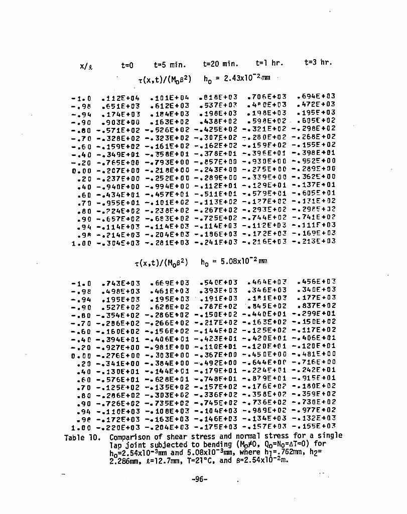
X/.t t=O t=5 min. t=20 min. t=l hr. t=3 hr.

-r(x, t) / (MoS 2 ) ho = 2.43xl0-2 ·mm

-1.0 .112E+04 .101E+04 .816f+03 .706E+D3 .694E+03 -.98 .651£+0'3 .612E+03 .537f+0?: .4"0£+03 .472E+03 -.94 .174E+03 .18 4E+ 03 .196E+03 .lQaE+03 .195£'+03 -.90 .903E+00 • 163£+02 ."38f+02 • 5913E+02 . .605£+02 -.60 -.571E+02 -.526£+02 -.425E+02 -.321E+02 -.298E+02 -.70 -.328E+02 -.323E+02 -.307j:+02 ~.28oE+02 -.266E+02 -.60 -.159£+02 -.161£+02 -.162E+02 -.159E'+02 -.155E+02 -.40 -.349E+01 -.~58E+01 -.376E+01 -.39f.E+ol -.396E+D1 -.20 -.765E+00 -.793E+00 -.857E+00 -.930E+OO -. 952E+0 0 0.00 -.207E+00 -.216E+00 -.243f+00 -.275E+00 -.289£+00

.20 -.237E'+OO -.25 2E+ 0 0 -.289£+ 00 -.339£+00 -.362£+00

.40 -.940f+00 -. 994E+0 0 -.112E'+01 -.129E+01 -.137£+01

.60 -.434E+Ol -.457£+01 -.511E'+Dl -.579E+C1 -.605£+01

.70 -.955E+Ol -.101£+02 -.113£+02 -.1~7E+02 -.1::t1E+02

.80 -.?24E+02 -.238F.+02 -.267[+02 -.293£+02 -.2gef+J2

.90 -.657E+02 -.683E+02 -.725E+02 -.744E+02 -.741E+02

.94 -.114E+03 -.ll"E+ 03 -.114E+03 -.112E+0 3 -.111f+03

.9~ -.214E+03 -.204£+03 -.186£+03 -.172E+03 -.169£+03 1.00 -.304~+03 -.281£+03 -.241F+03 -.216E+tJ3 -.213[+03

-1.0 .743E+03 .669£+03 .54Cf+03 .464E+0~ .456E+0'3 -.98 .498£+03 .461£+03 .393f+03 .346E+03 .340E+03 -.94 .195£+03 .195E+ 03 .• 191f+03 .1~lE+O~ .177£+03 -.90 .527E+02 .628E+02 .787E+02 .845E+02 .837£+02 -.80 -.'354£+02 -.286£+02 -.150f+02 -.440E+01 -.299f+Ol -.70 -.286£+02 -.266£+02 -.217E+02 -.163£+02 -.150£+02 -.60 -.160E+02 -.156£+02 -.144F+02 -.125£+02 -.117E+02 -.40 -.394E+01 -.406E+01 -.423E+01 -.420E+01 -."06E+01 -.20 -.927E-+00 -.981E+00 -.110E+01 -.120£+01 -.12of+01 0.00 -.276E+00 -.303E+00 -. 367E+0 0 -.450£+00 -.481E+00

.20 -.341E+00 -.384E+OO -·.492E+00 -.6,.r.E+or -.716£+00

." 0 -.l3D£+01 -.1"4E+ C 1 -.179E+01 -.224£"+(11 -.242£+01

.60 -.576E+Ol -.62 8E"'0 1 -.748F+01 -.879E+01 -.915£ +01

.70 -.125£+02 -.135E+02 -.157£+02 -.176£+02 -.180E+02

.80 -.286E+02 -.303E+02 -.336f+02 -.358E+O? -.359£+02

.90 -.726£+02 -.735E+02 -.745E+02 -.736E+02 -.730£+02

.94 -.110E+03 -.108E+03 -.104f+03 -.989E+0~ -.977£+02

.9lt -.172£+03 -.163E+03 -.146E+03 -.13r.£+03 -.132£+03 1.00 -.22oE+03 -.204E+03 -.175£+03 -.157£+U3 -.155E+O~

Table 10. Comparison of shear stress and normal stress for a single lap joint subjected to bending (Mo~O, Qo=No=~T=O) for ho=2.54xl0-3mm and 5.08xlO-3mm, where hl=.762mrn, h2= 2.286rnm, 1=12.7mm, T=21°C, and S=2.54x10-2m.

-96-

xl'l t=O t=5 min. t=20 min. t=l hr. t=3 hr.

a{x,t)/{MoS2) ho = 2.54x10-2mm

-1.0 -.286E+04 -.27 9E+ 04 -.267£+D4 -.252E+04 -.263E+04 -.98 -.170E+03 -.18GE +0'3 -.213[+03 -.229E+02 -.231£'+03 -.94 .157'f+03 .159E+03 .163E+03 .165E+03 .166E+03 -.90 .107E+03 .109E+03 .113E+03 .11 6E+U ~ .11f.E+03 -.80 ."29E+02 .42QE+02 .430E+02 .434[+ 0.2 • "36F+02 -.70 .192E+02 .190E+02 .186(+02 .183f+02 .183E+0? -.60 .e64E+01 • 875E+0 1 .854E+01 • e29E+01 • e23E+01 -.,. 0 .190E+Ol .190E+Ol .188[+01 .11j4E+01 .182E+01 -.20 ."07£+00 .409[+00 .412f+00 .412[+00 .410E+OO 0.00 .653£-01 • E5 5E-0 1 .658E-Ol .6r;2E-01 .643E-01

.2e -.907E-01 -.941[-01 -.102F+DO -.112E+OO -.116£+00

.40 -.504E+00 -.517E+OO -.547E+OO -. 5~ OE+O [1 -.591E+OO

.60 -.235E+01 -.2'3 8E+ 0 1 -.246F+Ol -.253[+01 -.254[+01

.70 -.503f+01 -.507F+01 -.515[+01 -.51~E+C1 -.517E+Ol

.80 -.106E+02 -.106[+02 -.105F+02 -.103E+02 -.102[+02

.90 -.207E+O'2 -.203[+02 -.195f+02 -.187E+02 -.186E+02

.94 -.238f+02 -.230E+02 -.215E+02 -.204E+02 -.C?02f+02

.9P. .473[+02 .,.94E+CC? .526E+02 .535E+02 .533E-4-02 1.00 .514[+03 .492E+03 .454f+03 .412E+0~ .lt2<:'E+03

a{x,t)/{Mos2) ho = 5 .08x10-2 rrrn

-1.0 -.207E+04 -.201£+04 -.193f+04 -.19UE+04 -.19"£+04 -.9~ -.309£+03 -.322E+03 -.343E+03 -.35SE+03 -.356E+03 -.94 .1lt8f+03 .148E+03 .147£+03 .145E+03 .14SE +03 -.90 .117E+03 .119£+ 03 .124f+03 .127[+03 .127[+03 -.80 .445E+02 .450[+02 .460[+02 .47 1(+02 .474f+02 -.70 .189E+02 .187E+02 .185£+02 • 184E+0 2 .184[+02 -.60 .856[+01 .840[+01 .806E+01 .777[+01 • 773[ +01 -.ltO .189£+01 .186E+01 .178E+Ol .167E+Ol .163E+01 -.20 .424F.+00 .1t23E+00 .416E+00 .397E+OC .385[+00 f).00 .669E-01 .66 OE- 0 1 .627E-01 .550E-01 .1t94£-Ol

.20 -.115£"+00 -. 12ltE+ 0 0 -.143F+00 -.166E+00 -.175[+00

.40 -.598[+00 -. 623[+() 0 -.680F+00 -.7~6E+OO -.749£+00

.60 -.261E+01 -.266[+01 -.274E+01 -.279E+01 -.279[+01

.70 -.536E+01 -.538E+Cl -.539E+01 -.5~3E+U1 -.529E+01

.80 -.107£+02 -.106E+02 -.103[+02 -.992E+Ol -.983[+01

.90 -.194E+02 -.189E+02 -.179£+02 -.171E+02 -.i69F+02 .9,. -.182E+02 -.171£+02 -.152f+02 -.140[+02 -.138E+02

.98 .674E+02 .679E+02 .682F+02 .673[+02 • E69E+02 1.00 .35~[+03 • 337E+ 03 .309r+03 .293F.+03 .291E+03

Table 10. Conti nued

-97-

xl! t=O t=5 min. t=20 min. t=l hr. t=3 hr.

(a) T(x,t)/{~T/a) h1 = 1. 27 I11Tl

-1.0 .343E'+02 .31ItE+02 .265E+02 .234E+02 .231£+02 -.98 .285f+02 .266E+02 .230E+02 .207E+02 .204E+02 -.94 .198F.+02 .190E+02 .175£+02 .162E+02 .160E+02 -.90 .137E+02 .136[+02 .132E+02 .127E+02 .125£+02 -.80 .562£'+01 .599E+01 .660£+01 .686E+01 .683f+Ol -.7r .235E'+01 .267E+01 .328E+Ol .371E+Ol .375E+01 - .,6 0 .101E+01 .121E+01 .163E+ 01 "200E+01 • 207E+01 -.40 .206£+00 • 265E+ CO .'+09~+00 .5~3E+oO .634E+00 -.20 .451£-01 • 594E- 0 1 .989E-01 .158E+00 .181£+01] 0.00 .998E-12 .699E-12 ."56f-12 .366£-12 • 510£-12

.20 -.'+51E-01 -.594E-01 -.989=-01 -.158E+00 -.181E+OO • ft 0 -.206£+00 -.26 t;E+ 0 0 -.409F'+00 -.5~3F+OO -.634£+00 .60 -.101F+01 -.121E+ 01 -.163E+Ol -.200E+01 -.207f+01 .70 -.235E'+01 -.2£7E+01 -.328f+Ol -.371E+rl -.375f"'01 .80 -.562£+01 -.599E+C1 - .66 oE+Cl -.6~6E+01 -.6~3F+01 .90 -.137E+02 -.136£+02 -.132£+02 -.127£+D2 -.125~+02 .9ft -.198E+02 -.19 OE+ 02 -.175F+02 -.162E'+C2 -.160f+02 .98 -.285E+02 -.266£+02 -.230£+02 -.207£+02 -.204E+D?

1.0(! -.343£+02 -.311,£+02 -.265E+02 -.23ftE+O? -.231E+02

(b) T(x,t)/(~T/a) h1 = 2.286 nm

-1.0 .391E+02 .359E+02 .302f+02 .267E+02 .263£ + 02 -.98 .333E+02 .309E+02 .267f+02 .2ftOE+02 .236f+02 -.94 .241E'+02 .231E+02 ~210E+02 .193E+02 .190E+02 -.90 .175E+D2 .172E+02 .164(+02 .156E+02 .154E+02 -.80 .798[+01 • 836E+0 1 .894F+01 .910E+U1 .904£+01 -.70 .371f+D1 .1t11E+01 • "66f+01 .532E+01 .534F+01 -.60 .176f+Dl .205E+01 .26Itf+Ol • 311E+0 1 .317£+01 . -."0 .1,33£+00 .540E+00 .788E+00 • 106E+01 .112E+Ol -.20 .111E+00 .142f+00 .221E+00 .326E+00 .360£+00 0.00 -.525E-12 -.174E-11 .665f-13 .88!.'£-12 -.724E-12 .20 -.111£+00 -.142E+00 -.221f'+00 -.326E'+O(l -.360£+00 .40 -.433E+0 0 -.5" OE+O 0 -.788E+00 -.106E+01 -.112E+01 .60 -.176E+Ol -.205E+D1 -.264E+01 -.311£+01 -.317f+01 .7 C -.371£+01 -.411E+01 -.466f+01 -.532£+01 -. 534~+Ol .80 -.798E+01 -.836£+01 -.894f+Ol -.910[+01 -.904E+01 .90 -.175£+02 -.17 2E+ 0 2 -.164E+02 -.156£+02 -.154E+O? .94 -.241E+02 -.231E+02 -.210f+02 -.193E+02 -.190E+02 .98 -.333£+02 -.309£+02 -.267E+02 -.240E+02 -.236£+02

1.00 -.391£+02 -.359£+02 -.302E+02 -.267E+02 -.263[+02

Table 11. Comparison.of shear stress and normal stress resulting from a temperature increase (~TIO, Mo=No=Qo=O) in a cover plate for h1=1.27mm and 2.286mm, where h2= 2.286mm, 1=12.7mm, h?=.1016mm, T=21°C, and a= (2.54x10- 2m)(5/9°C)1 4.448N).

-98-

X/t t=O t=5 min. t=20 min. t=l hr. t=3 hr.

(c) a(X,t}/(6T/S) h1 = 1.27 mm

-1.0 .115E+02 .106E+02 • «:I56f+Ol .6RUE+Ol • e70E+Ol -.«:18 .4g8f+Dl .481E+ 0 1 .448F+Ol .422£+01 • 417E+0 1 -.94 .456E+00 .524£+00 .625E+00 .65c:lf+00 .655E+00 -.90 -.557[+00 -.488E+00 -.3'64f+OO -.2R7E+OO -.280£+00 -.80 -.719£+00 -.686E+OO -.61C?E+OO -.51) 2E+ [l.O -.551£+00 -.70 -.509£+00 -.500E+00 -.475E+00 -.447E+OO -.439£+00 -.£>0 -.324F+OO -.326£+ 0 0 -.~24E+00 -.316E+00 -.:!12E+OO -.40 -.116£+00 -.121E+OO -.131E+00 -.137£+00 -.13Bf+OO -.20 -.416E-Ol -.446E-Ol -.514E-01 -.5~5E-O~ -.603E-Ol 0.00 -.241£-01 -.262E-Ol -.314f-01 -.377E-01 -.396f-Ol

.20 -.416E-01 -.446£-01 -.514E-Ol -.5~5E-C1 -.60"!E-Ol

.40 -.116£+00 -.121£+00 -.131E+00 -.137E'+OO -.138£+00

.60 -.324£+00 -. 326E+U () -.324E+00 -. 31G£: +() () -.31215:+00

.70 -.509E+00 -.500£+00 -.475E+00 -.447~+OO -.43QE+QO

.80 -.719f+00 -.686E+00 -.61C?E+OO -.5E-2E+r!) -. 551E+ 00

.gl'l -.557£+00 -.4813£+(;0 -. "364£+00 -.287£+00 -.280E+00

.94 .458£+00 .524E+00 .625£+00 .659E+00 • 655E+0 0

.ge .498E+Ol • 481E+- 01 .448E+01 .422E+01 .417E+Ol 1.00 .115E+02 .108E+02 • 95~F+01 .8'301:+01 .870£+01

(d) a(x,t)/(6T/S) h1 = 2.286 nun

-1.0 -.133E+02 -.125£+02 -.112E+02 -.lr3£+02 -.102f+02 -.ge -.703f+01 -.676E+01 -.625£+01 -.5.137E+Ol -.580f+Ol -.94 -.151E+Ol -.156E+Ol -.162E+Ol -.161£+01 -.160£+01 -.90 .248E+00 .158£+00 .538E-02 -. 750E-O 1 -.789£-01 -.80 .936E+00 .883E+00 .760f+00 .698£+00 .685E+00 -.70 .776E+00 • 754E+0 0 .703E+00 .653£+-00 .642E+00 -.60 .563£+00 .55 BE+ 0 0 .542£+00 .51 Q £+00 .511E+DO -.40 .262£+00 .268£+00 .279f+00 • 2R4£+ 00 .283E+OO -.2D .125E+00 .131E+00 .144F.+00 .155£+-0£1 .157~+OO

0.00 .673E-Ol .926£-01 .104E+00 .111£+-00 .120F+00 .20 .125£+00 .131£+00 .14 '+(+ 0 0 .155E+n(l .157"E+00 .40 .262E+00 .268E+00 .279E+00 .2~4E+cr .283F+00 .60 .563E+OO .558£+00 .542f+00 .519E+00 .511E+-00 .70 .776£+00 .754£+00 .703E+00 .&53E+00 • 642E+0 0 .60 .Q3f.E+00 .883£+00 .780E+00 .698E+00 .685£+00 .90 .248E+00 .158E+00 .538E-02 -.75CE-Ol -.789£-01 .94 -.151E+01 -.15 6E+0 1 -.162E+Ol -.161E+01 -.160£+01 .98 -.703E+Ol -. 676E+0 1 -.625E+Ol -.587£+01 -.580E+01

1.00 -.133E+02 -.125E+ 02 -.112Et02 -.103E+02 -.102£+02

Table 11. Continued

-99-

xl! t=O· t=5 min. t=20 min. t=l hr. t=3 hr.

T(x,t)/(Mo/S2 ) REISSNER THEORY

-1.0 .488E+03 .43 aE + 03 .~51[+O3 .301E+03 .29f.E+03 -.9a .3f;O~+O~ • ~~ DE + 03 .276E+03 .240E+0~ • 231SF. + 03 -.94 .181f+03 .175E+03 .161E+03 .147E"+03 .145E+03 -.90 .796(+02 • 8~5E+02 .878E+02 .864[+02 .851F+02 -.80 -.~01'=+01 -.237£+01 °.965£+01 .16 O E+02 .174£+02 -.70 - .182£ + 02 -.147E+02 -.755£+01 -.165E+01 -.780E:+00 -.60 -.130F+02 -.116£+02 -.836f+Ol -.491E+0·1 -.414E+01 -.40 -.41E:f+Ol -.40 8E+ 01 -.371E+Ol -.293E+Ol -.258£+01 -.20 -.!17E+01 -.123E+01 -.130F+Ol -.124[+01 -.115E+01 0.00 -.1.41F+0(} -.504E+0(! -.f.51E+00 -. 810E+ (1(1 -.8La7E+OO

.20 -.633F+OO -.75 8E + 00 -.107E+Ol -.147E+(ll -.161£+01

.ft 0 -.21PF+01 -. 252E+ 01 -.332E+Ol -.423E+01 -.448E+Ol

.6 (l -.8lt8 r +Ol -. 9~7f+0 1 - .112E +0 2 -.129£+02 -.132£+02

.7 C -.170£+07 -.lR2E+02 -.207E+02 -.2?4E+D2 -.226E+02

.6 {) -.344f+02 -. 357E+ 02 -.379f+02 -·.367£+02 -.385£+02

.90 -.717E+02 -.710E+02 -.f89E+02 -.661E+02 -.654F+02

.94 -.972£+02 -. ~L. Of + 02 -.874f+02 -.817E+02 -.806[+02

.9~ -.134r:+03 -.12f>E+C3 -.111F+03 -.101E+O~ -.996E+02 1.00 -.1~9F+03 -.147E"+03 -.126E"+03 -.113E+0?- -.111E+03

T(x,t}/(Mo/6 2 ) CLASSICAL THEORY

-1.(1 .428F+03 • ~l\2E+03 .303f+03 .25~E+03 .254f+03 -.98 .299F+03 • 27 3f + (j:3 .227E+03 .lg8E+03 .194E+03 -.91. .121E+03 .11QE+O~ .114E+03 .106E+03 .104£+03 - .9Q .362£+02 .426E"+02 .520£+02 .545E+02 .538E+02 -.80 .483f+Ol .I'44E+01 .154[+02 .20?E+02 .20Sf+0? -.70 .778E+01 .qlLaE+01 .121E+02 .148E+D2 .152E+02 -.6G .370E+01 .459E+C!1 .657£+01 .855£+01 .897E+01 -.40 .441f+OO .673E+OC .12qE+01 .214E+Oj .242£+01 -.20 .721E-01 .12 OE+ 0 0 .267E+00 .520E+00 .637E+00 0.00 -.785E-02 -.134E-01 -.299E-01 -.565~-01 -.EE3E-01

.20 -:-.122£+ 00 -.196E+00 -.411E+00 -.746£+00 -.884£+00

.4(1 -.7135£+00 -.113E+01 -.195£+01 -.2CJSE+Ol -.324~+01

.60 -.'+99E+01 -.619E+01 -.868£+01 -.10RE+02 -.112E+02

.70 -.130F+0~ -.149[+ 0 2 -.184E+02 -.207E+n2 -.209£+02

.80 -.342E+02 -.36 OE+ 0 2 -.387E+02 -.397E+02 -.39~E+02

.9 (j -.800E+02 -.7A5E+02 -.750E+02 -.713E+02 -.704E+02

.94 -.107f+03 -.103E+03 -.943[+02 -.8 7 5E+02 -.863[+02

.98 -.143[+03 -.134E+03 -.118f+03 -.1D7E+O:! -.105E+03 1.00 -.168£+03 -.155E+03 -.133£+03 -.118£+03 -.117£+03

Table 12. Comparison of shear stress and normal stress for a single lap joint subjected to bending (Mo10), No=Qo=~T=O) for Reissner and for classical plate theories, where h1= .762mm, h2=2.286mm, ho=.1016mm, !=12.7mm, T=21oC, and S=2.54xl0-2m.

-100-

x/R. t=O t=5 min. t=20 min. t=l hr. t=3 hr.

a(x,t)/(Mo/s2 ) REISSNER THEORY

-1.0 -.149E+04 -.145E+0Z. -.140(+04 -.137E+04 -. 137 E" + 0 Z. -.98 -.386E+03 -.393E+03 -.405E+03 -.411£+03 -.412(+03 -.94 .111£+03 .107E+03 .~98f+02 .954E+02 .950 E+02 -.90 .123£+03 .124E+03 .127£+0'3 .1?eE+O:! • 128£+03 -.80 .488£+02 .499E+02 .520f+02 .537E+02 .540E+02 -.70 .191(+02 .191E+02 .193£+02 .197E+02 .198[+02 -.60 .B13E+01 .796£+01 .766E+01 .150E+01 .752E+01 -.40 .j76E+Ol .168E+01 .150F+01 .132E+Ol .129E+01 -.20 .417E+00 .400£+01) .353E+00 .284(+00 • 26 OE +0 0 O.oc .573E-01 • ltC? 6£-0 1 .272(-01 -.8"39£-02 -.241£-01

.2 C -.173(+00 -.192E+00 -.235F+00 -.282£+OC -.295£+00

.40 -.767E+00 -.807E+00 -.888£+00 -.950E+OC -. 956E +00

.60 -.294E+01 -. 297E+0 1 -.300(+01 -.297£+01 -.294F+01

.70 -.566£+01 -.561E+Ol -.548[+01 -.528[+01 -.?22E"'01

.80 -.107(+02 -.104E+02 -.994[+01 -.94~E+Ol -.938F+01

.90 - .172£+02 -.165E+02 - .15 3E"+02 -.144£+~? -.143f+0?

.94 -.918F+Ol -.~OOE+Ol -.601E+01 -.49~E+rl -.4c:t3E+01

.98 .747£+02 .737£+02 .715F+02 .693£+02 .68PF+02 1.00 .243E+03 .231E+03 .211E+03 .199E+0::' .1~e.E+03

a(x,t)/(Mo/S2 ) CLASSICAL THEORY

-1.0 -.156£+04 -.152E+04 -.146F+04 -.14-::rE+04 -.143£+04 -.9a -.739[+03 -.732£+0"3 -.720(+03 -.715E+03 -.715E+03 -.94 .122[+03 .109E+03 .869E+02 .754[+C2 .745(+02 -.90 .322£+03 .315E+03 .303f+03 .296£+03 .296£+03 -.80 .773£+02 .821E+02 .906[+02 .9«;7E+02 • 962E+0 2 -.70 -.147[+02 -.145[+02 -.140f+02 -.133E+02 -.131E+02 -.60 -.!t91E+01 -.562E+01 -.692E+01 -.776E+01 -.782£+01 -.40 .100E+00 .968£-01 .681E-Ol .3A4E-02 -.161E-01 -.20 -.281E-01 -.415E-01 -.773E-01 -.128E+00 -.147E+00 0.00 -.674£-02 -.121E- 0 1 -.290:-01 -.602E-01 -.757£-01 .20 -.279E'-01 -.431£-01 -.839f-Ol -.140£+0(1 -.158[+00 .It 0 -.213E+00 -.276E+OO -.414F+00 -.53QE+OO -.559£+00 .60 -.561E+OO -.704E+00 -.960£+00 -.109£+01 -.108E+01 .70 -.247E+01 -. 277~+01 -.32DE+01 -.326£+01 -.31QE+01 .80 -.205f+02 -.203E+02 -.196E+02 -.186£+02 -.184E+02 .90 -.391E+02 -.360E+02 -.309E+02 -.21\2E+O? -.280E+02 .94 .314E+01 .496E+Ol .757E+01 .83~E+01 .822E+Ol .96 .122E+03 .117E+03 .108E+03 .102£+03 .101f+03

1.00 .218E+03 .206£+03 .187£+03 .176E+03 .174E+03

Table 12. Conti nued

-101-

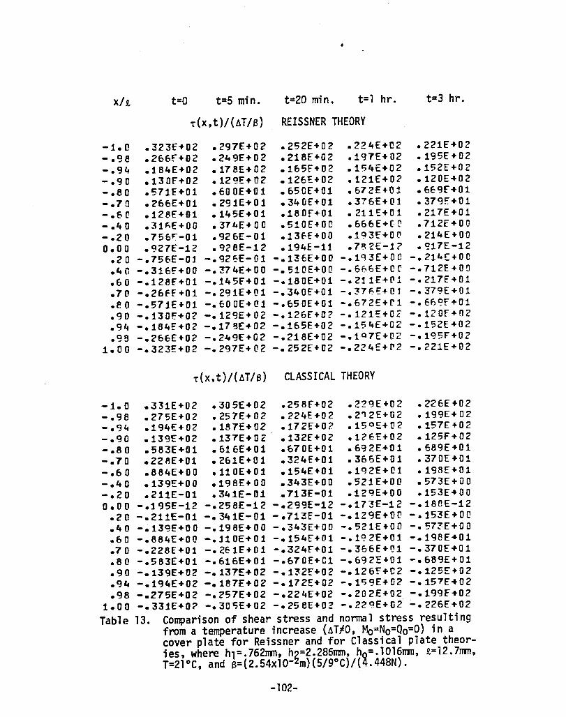
xh. t=O t=S min. t=20 min. t=l hr. t=3 hr.

T{x,t)/{l1T/S) REISSNER THEORY

-1.0 .323£+02 .297E+02 .252E+02 .224E+C2 .221E'+02 -.ge .266f+02 • 2l+ 9£+ 0 2 .218E+02 .197E+02 .195£+02 -.94 .184E+02 .178E+02 .165F+02 .154£+02 .152£+02 -.90 .130£+02 .129E+ 02 .126£+02 .121E+02 .120E+02 -.80 .571f+Ol .600E+Ol .650[+01 .672E+01 .669£+01 -.70 .266E+01 .291E+Ol .340£+01 .376E+01 .379f+01 -.Ge .12Bf+01 .145£+01 .180f+01 • 211 '::+01 • 217E +0 1 -.40 .31F.E+OO .374E+00 .510E+00 • 666E+( ~ .712f+OO -.20 .756~-01 .926E-01 .13£-f+00 .1~3f+O(l .214E+00 0.00 .927E-12 .928E-12 .194E-11 .7~2E-12 • C117E-12

.20 -.756E-01 -.92 E-E- 01 -.136E+00 -.1Q3[+OC -.214(+00

.4(1 -.316f+OO -. 374E+ 00 -.510E+OQ -.6&6E+C[ -. 712E + 0 0

.60 -.128£+01 -.145£+01 -.180[+01 -.211E'+£l! -.217E+01

.70 -.26ff+Ol -.291E+01 -.340£+01 -.::t7f:,E+01 -.379E"'01 • f! 0 -.571E+01 -.600E+01 -.650£+01 -.672E+[,1 -. 6f,~f+01 .90 -.130~+02 -.129£+02 -.126f+02 -.121~+OZ -.120£+02 .94 -.184f+02 -.17~[+02 -.165E+02 -.154E+02 -.152£+02 .98 -.266[+02 -.249(+02 -.218[+02 -.l Q 7[+P.2 -.19SF+02

1.00 -.323£+02 -. 297E+ 02 -.252£+02 -.224£+('2 -.221E+02

T(x,t)/{l1T/S) CLASSICAL THEORY

-1.0 .331E+02 .305E+02 .258£+02 .229E+02 .226E+02 -.98 .275E+02 • 257E+ 0 2 .224£"'02 .2'12E+02 .199E+02 -.94 .194£+02 .187E+02 .172f+0? .15 0 £+02 .157E+02 -.90 .139E+02 .137E+02 .132f+02 .126£+02 .125f+02 -.80 .583E+01 • 616E+ 0 1 .670E+Ol .692E+01 .689E+01 -.70 .228E+01 • 261E+0 1 .324E+01 .366£+01 • 370E +01 -.60 .864£+00 .110E+Ol .154E+Ol .lQ2E+Cl .198E+01 -.40 .139E+0 0 .198£+00 .343E+00 .521E+OO • 573E+0 0 -.20 .211E-01 .341E-Ol .713E-tll .12QE+OO .153E .. 00 0.00 -.195E-12 -.258E-12 -.299E-12 -.173£-12 -.180E-12

.20 -.211E-01 -.341E-01 -.71:3F-Ol -.129E+O[l -.153E+OC!

.40 -.139E+00 -.198£+00 -.'343£+00 -.521£+00 -. ?7?E+O 0

.60 -.664£"'00 -.11 OE+O 1 -.154£+01 -.1C?2£+01 -.198["01

.70 -.226[+01 -. 261E+0 1 -.324£+01 -.366E+1)1 -. 370E+0 1

.80 -.583[+01 -.616£+01 -.670E+Cl -.692::+01 -.689E+01

.90 -.139£+02 -.137E+02 -.132£"+02 -.126F+C2 -.125E+02

.94 -.194£+02 -.187£+02 -.172E+02 -.1'59£+02 -.157E+02

.98 -.275E+02 -.257E+02 -.224[+02 -.202E+02 -.199f+02 1.00 -.331E+0? -.30'5[+02 -.258£+02 -.229E+02 -.226£+02

Table 13. Comparison of shear stress and normal stress resulting from a temperature increase (l1T;O, Mo=No=Qo=O) in a cover plate for Reissner and for Classical plate theor-ies, where hl=.762mm, h~=2.286rnm, h~=.1016rnm, R.=12.7nm, T=21oC, and S=(2.S4x10- m)(S/9°C)/( .448N).

-102-

xl! t=O t=5 min. t=20 min. t=l hr. t=3 hr.

a{x,t)/{l1T/s) REISSNER THEORY

-1. 0 .242E+02 .226E+02 .199f+02 .181E+02 .179F+O? -.98 .825£+01 .800E+01 .749E+01 .70'+[+01 .E96£+01 -.94 -.301£+00 -.145E+0 0 .111E+00 .236E+OO .239E+OO -.90 -.152f+01 -. 139E+0 1 -.115E'+01 -.986E+OO -.96f~+OO -.80 -.125[+01 -.120E+01 - .109E+01 -.993E+00 -.974E+00 -.70 -.739E+00 -.731E+00 -.706t+00 -.669E+00 -.65Rf+00 -.60 -.405E+00 -.412E+00 -.421f+00 -.417£+00 -. 413E +00 -.40 -.111E+00 -.119£+00 -.135f+00 -.148E+00 -.150E+00 -.2(1 -.310E-01 -.35 OE-O 1 -.440E-Ol -. 53 ~E-Ol -.566E-Ol 0.00 -.151E-01 -.177E-Ol -.239E-01 -.317f.-nl -.344f-Ol

.20 -.310£-01 -.350E-01 - .44 OE-01 -.539E-CJ1 -.566E-01

.4 (1 -.111£+00 -.119E+00 -.135£+00 -.14R£+OO -.150E+00

.60 -.405E+00 -.412E+OO -.421E+00 -.417E+OC -.413E+00

.70 -.739f+OO -.731£+00 -.706E+00 -.6C;9£+on -. 658f+0~

.80 -.125F+Ol -.120E+01 -.109E+01 -.9Q!.E+C{) -. <374E+0 C

.90 -.152F.+Ol -.139E+Ol -.115E+Ol -.9Rf,f+OO -.966E+00

.94 -.:!01E+OO -.145!:+00 .111E+00 .236E+OO .23~E+OO

.9!' .825E+01 .80DE+01 .749E+01 .704E+01 .696£+01 1.00 .242£+02 .22EE+02 .1C?9E+02 .181£+02 .17C?E+02

a{x,t)/(l1T/s) CLASSICAL THEORY

-1.0 .191£+02 .176E+02 .151E+02 .135E+02 .133f+02 -.9R .123E+02 .115E+0 2 .101f+0? .918f+01 .905E+Ol -.94 .191E+01 .206E+01 .226E+01 .226£+01 .223E+01 -.90 -.296E+01 -. 253E+0 1 -.180£+01 -.141£+01 -.13':1E+01 -.80 -.259E+01 -.25 OE+ 0 1 -.228E+Ol -.2!l6E+01 -.202E+01 -.70 -.582E+00 -.631E+00 -.698f+00 -.699E+00 -.685£+00 -.60 -.150£+00 -.182E+00 -.240£+00 -.271E+00 -. 270E+0 0 - .40 -.349£-01 -.455E-01 -.690£-01 -.910E-01 -.945f-01 -.20 -.506E-02 -. 71' 2£-02 -.152£-01 -.254E-01 -.286£-01 0.00 -.156£-02 -.274E-02 -.629E-02 -.125E-01 -.155f-Ol

.20 -.506F-02 -.782E-02 -.152E-01 -.254E-U1 -.26Rf-01

.40 -.349E-01 -."55E-01 -.690E-01 -.910E-01 -. «:l45E-!J1

.60 -;'150E+00 -.16ZE+DO -. Z40f+OO -. Z71E+OO -.270£+00

.70 -.582E'+00 -.631E+00 -.698f+00 -.699E+OO -.685'=+00

.80 -.259f.+01 -.25 OE+ 0 1 -.228[+01 -.206E+01 -.202E+01

.90 -.296E+Ol -.253£+01 -.180F+Ol -.141E+01 -.139f+01

.94 .191E+01 .206£+01 .226F+01 .226£+01 .223E+01 .98 .123E+02 .115E+02 .101E+02 .918E+01 .905E+01

1.00 .191£+02 • 176E ... 02 .151f+02 .1~5E+02 .133£+02

Table 13. Continued

-103-

TillE in Seconds

0.00 1.00 3.00 5.00

10.00 15.00 20.00 25.00 30.00 35.00 40.00 45.00 50.00 55.00 60.00 65.00 70.00 75.00 80.00 85.00 90.00 95.00

100.00 150.00 200.00 250.00 300.00 350.00 400.00 450.00 500.00 550.00 600.00 650.00 700.00 800.00 900.00

1000.00 1100.00 1200.00 1300.00

Data From Fig. (14) 1 Unit=.01245 em

• 630000E+01 • 650000E+01 • 660000E+01 • 663000E+01 • 672000E+01 • 678000E+01 .683000E+01 .687000E+01 • 690000E+01 .692500E+01 • 695000E+01 .696500E+01 .698000E+01 .700000E+01 .701500E+01 .702500E+01 .703500E+01 .704500E+01 .705500E+01 .706500E+01 .707500E+01 .708500E+01 .709500E+01 .713000E+01 • 718500E+01 .723000E+01 • 725000E+01 • 727000E+01 • 729000E+01 • 732000E+01 • 733000E+01 .735500E+01 • 737000E+01 • 739000E+01 .741000E+01 .743000E+01 • 745000E+01 • 747000E+01 • 749000E+01 • 750500E+01 • 752000E+01

Calculated Value Using Eqn. 022)

.630000E+01

.650766E+01

.658218E+01

.663721E+01 • 672743E+01 • 678505E+01 • 682846 E+O 1 .686415E+01 • 689468E+01 .692126E+01 • 694460E+01 .696520E+01 • 698346E+01 .699971E+01 .701422E+01 .702725E+01 .703899E+o1 .704963E+01 .705930E+01 .706816E+01 .707629E+01 .708381E+01 .709080E+01 • 71 4284E+o1 • 718049E+01 • 721290E+o1 • 724222E+01 • 726910E+01 • 729380E+01 • 731653E+01 • 733744E+01 • 735668E+01 • 737438E+01 • 739067E+01 • 740566E+01 • 743214E+01 • 745455E+01 • 747353E+01 • 748960E+01 • 750320E+01 .751472E+0l

THE SUM OF THE SQUARES IS • 145251E-02 THE ~XIMUM DIFFERENCE IS .178230E-0l (T=3 sec.)

TABLE 15. DATA FIT OF CREEP CURVE

-104-

Time In T(O,t) for T(O, t) for T(O,t) for Seconds Gene ra ti on Pe r Generation Per Generation Per

Cycle Unit Time Uni t Time °C (No coupling) (Hith Coupling)

°C °C

0 22.000 22.000 22.000 100 22.940 22.951 22.873 200 23.804 23.816 23.738 300 24.536 24.546 24.474 400 25.141 25.151 25.086 500 25.639 25.648 25.590 600 26.050 26.057 26.005 700 26.387 26.393 26.347 800 26.664 26.670 26.629 900 26.892 26.897 26.861

1000 27.080 27.084 27.052 1100 27.234 27.237 27.210 1200 27.361 27.364 27.340 1300 27.466 27.468 27.447 1400 27.551 27.553 27.536 1500 27.622 27.623 27.609 1600 27.680 27.681 27.668 1700 27.728 27.729 . 27.718 1800 27.767 27.768 27.759 1900 27.799 27.800 27.792 2000 27.826 27.826 27.820 2100 27.848 27.848 27.843 2200 27.866 27.866 27.862 2300 27.880 27.881 27.877 2400 27.893 27.893 27.890 2500 27.903 27.903 27.901 2600 27.911 27.911 27.910 2700 27.918 27.918 27.917 2800 27.923 27.923 27.923 2900 27.928 27.928 27.928 3000 27.931 27.932 27.932 3100 27.935 27.935 27.935 3200 27.937 27.937 27.938 3300 27.939 27.939 27.940 3400 27.941 27.941 27.942 3500 27.942 27.942 27.944 3600 27.944 27.943 27.945 3700 27.944 27.944 27.946 3800 27.945 27.945 27.947 3900 . 27.946 27.946 27.947 4000 27.946 27.946 27.948

TABLE 16 - COMPARISON OF TEMPERATURE PROFILE FOR THREE DIFFERENT SOLUTIONS OF THE ENERGY EQUATION. CYCLING FREQUENCY IS 10 HERTZ.

-105 ..

Time In T(O,t) for T(O,t) for T(O,t) for Seconds Generation per Genera ti on pe r Generation per

Cycle Unit Time Uni t Time °C (No Coupling) (~ith Coupling)

°C °C

0 22.000 22.000 22.000 100 30.871 30.884 30.808 200 39.044 39.057 38.981 300 45.963 45.976 45.906 400 51.689 51.700 51.637 500 56.404 56.414 56.357 600 60.283 60.291 60.241 700 63.473 63.481 63.437 800 66.098 66.104 66.065 900 68.256 68.261 68.228

1000 70.031 70.036 70.007 1100 71.492 71.495 71.470 1200 72.693 72.696 72.674 1300 73.680 73.683 73.664 1400 74.493 74.495 74.479 1500 75.161 75.163 75.150 1600 75.711 75.712 75.701 1700 76.163 76.164 76.155 1800 76.535 76.535 76.528 1900 76.840 76.841 76.835 2000 77 .092 77 .092 77 .088 2100 77 .299 77.299 77 .296 2200 77 .469 77 .469 77 .467 2300 77.609 77 .609 77 .608 2400 77.724 77 .724 77.723 2500 77.819 77.819 77.819 2600 77 .896 77 .897 77 .897 2700 77.961 77 • 961 77 .962 2800 78.013 78.013 78.015 2900 73.057 78.057 78.058 3000 78.092 78.092 78.094 3100 78.121 78.121 78.124 3200 78.146 78.146 78.148 3300 78.165 78.165 78.168 3400 78.182 78.182 78.185 3500 78.195 78.195 78.198 3600 78.206 78.206 78.209 3700 78.215 78.215 78.218 3800 78.223 78.223 78.226 3900 78.229 78.229 78.232 4000 78.234 78.234 78.237

TABLE 17 - COMPARISON OF TEMPERATURE PROFILE FOR THREE DIFFERENT SOLUTIONS OF THE ENERGY EQUATION. CYCLING FREQUENCY IS 50 HERTZ.

-106-

10 HERTZ

Time In T(O,t) for T(O,t) for T(O,t) for Seconds Heat Gen. Heat Gen. Per Heat Gen. Per

Per Cycl e Unit Time Unit Time ( DC) (No Coupling) (Coupling)

0.0000 22.000 22.000 22.000 .0100 22.000 22.003 21.795 .0200 22.000 22.003 21.673 .0300 22.000 22.003 21.671 .0400 22.000 22.003 21.791 .0500 22.000 22.003 21.985 .0600 22.001 22.004 22.180 .0700 22.001 22.004 22.301 .0800 22.001 22.004 22.302 .0900 22.001 22.004 22.183 .1000 22.001 22.004 21 .989

50 HERTZ

0.0000 22.000 22.000 22.000 .0020 22.000 22.002 21.805 .0040 22.000 22.003 21.683 .0060 22.001 22.004 21.679 .0080 22.001 22.004 21.795 .0100 22.001 22.004 21.985 .0120 22.001 22.004 22.177 .0140 22.001 22.005 22.297 .0160 22.001 22.005 22.300 .0180 22.002 22.005 22.183 .0200 22.002 22.005 21.992

TABLE 18. Cor~PARISON OF THREE SOLUTIONS OF THE ENERGY EQUATION FOR TH1ES DURING THE FIRST CYCLE.

-107-

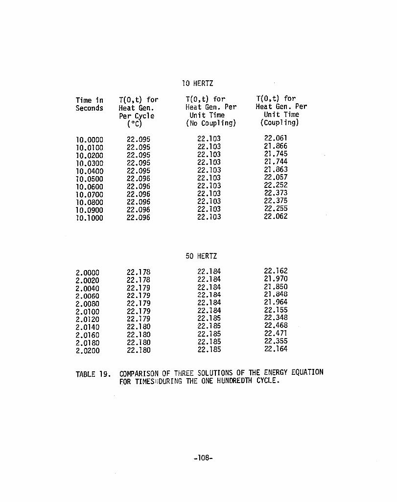
Time in Seconds

10.0000 10.0100 10.0200 10.0300 10.0400 10.0500 10.0600 10.0700 10.0800 10.0900 10.1000

2.0000 2.0020 2.0040 2.0060 2.0080 2.0100 2.0120 2.0140 2.0160 2.0180 2.0200

T(O,t) for Heat Gen. Per Cyc1 e

( °C)

22.095 22.095 22.095 22.095 22.095 22.096 22.096 22.096 22.096 22.096 22.096

22.178 22.178 22.179 22.179 22.179 22.179 22.179 22.180 22.180 22.180 22.180

10 HERTZ

T(O, t) for Heat Gen. Per Unit Time

(No Coupling)

22.103 22.103 22.103 22.103 22.103 22.103 22.103 22.103 22.103 22.103 22.103

50 HERTZ

22.184 22.184 22.184 22.184 22.184 22.184 22.185 22.185 22.185 22.185 22.185

T(O, t) for Hea t Gen. Per

Unit Time (Coupling)

22.061 21.866 21. 745 21. 744 21.863 22.057 22.252 22.373 22.375 22.255 22.062

22.162 21. 970 21.850 21.848 21.964 22.155 22.348 22.468 22.471 22.355 22.164

TABLE 19. COMPARISON OF THREE SOLUTIONS OF THE ENERGY EQUATION FOR TIMESllDURING THE ONE HUNDREDTH CYCLE.

-108-

~ _l i_

I lh, (l) , I x oCt:) (2.)

Tho h2.

tal

cr

1..1 1.. L :Jt t '"

Figure 1. The geometry of the bonded joint. Figure (a) shows the single lap joint, figure (b) the cover plate, and figure (c) the kinematics of the adhesive layer.

-109-

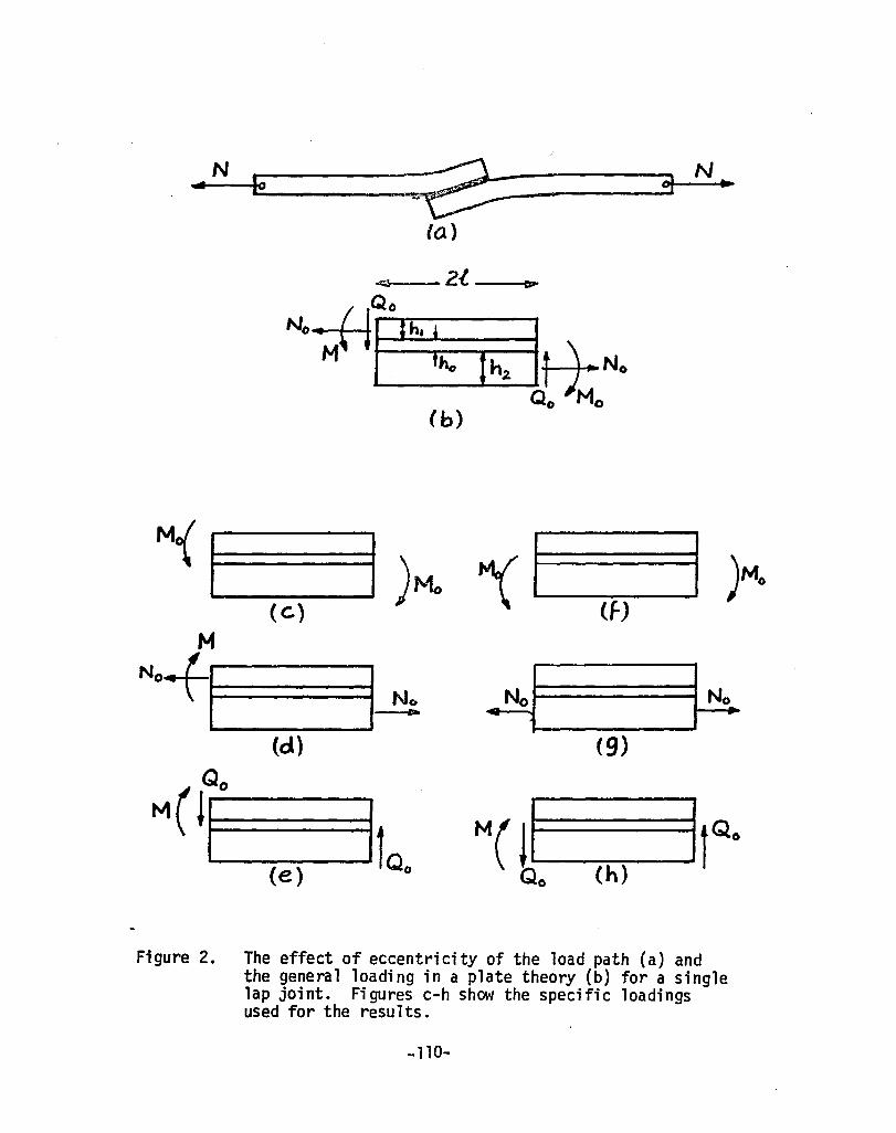
N ...

M.(l M

N@+I

Qo

~(ll

Figure 2.

~ 01 N JO ~

ta)

I )Mo ~l I )M. (c.) (f)

I~ 4

NoJ I No.

(d) (9)

(e) Ifao M( II

Qo (h) IrQ·

The effect of eccentricity of the load path (a) and the general loading in a plate theory (b) for a single lap joint. Figures c-h show the specific loadings used for the results.

-110-

Figure 3.

_.f.

hi L

-~

(a) A ~

l ---+ Q (l)

"(~)f } f g;, -'

N,ll) (l)

f >'

_J ~

l a

he, "t"

~ '2

Nz.{-l hL (2)

Qz.(-l)

(b)

-)(...

~

In figure (a) the elements used for the equilibrium equations are shown. Figure (b) shows the elements used for relations (51-53) that replace the boundary conditions.

-111-

_21_

J

7l

h, I I

T r

~T

o

h, = 1·21 mm.

h,=Z·2.80mm.

-0·5

: I ho Iha

1

t

Figure 4. Distribution of the nonmal stress resulting from a temperature increase in a cover plate for varying values of upper plate thickness hl. The other para­meters are: h2=2.286mm, ho=.1016mm, t=12.7mm, and B= (2.54xlO-2m)2(5/9°C)/(4.448N).

-112-

-z; (x~o) (LlT/(3)

20

10

-1

_21_

I : ho

T

o

h, ::. 2·21Jh mm.

h,::. o· 7l:J2 him.

-o-s xli

•

o

I

t

Figure 5. Distributions of the shear stress resulting from a temperature increase in a cover plate for varying values of upper plate thickness h1. The other para­meters are: h2=2.286mm, hQ=.1016mm, 1=12.7mm, and e= (2.54x10-2m)2(5/9°C)/(4.448N).

-113-

-100

T(x,lht:) ( No 1131

)

_ZDO~~ __ ~~~~ __ ~~ __ ~~~~~ ~J o I

Figure 6. Distribution ,of shear stress in. a single lap joint subjected to'bending where h1~1.27mm, h2=2.286mm, ~o=.1016rnm, t=12.7mm, T=21°C, and a=2.54x10- 2m.

-114-

.3()0

a-(x.o) CM" /P2)

200

100

~10o

-200

-300

-400

Figure 7. Distribution of normal stress in a single lap joint subjected to bending where hl=1.27mm, h2=2.286mm, ho=.1016mm, i=12.7mm, T=21oC, and S=2.54xlO-2m.

-115 ..

2'00 , -a-{-.(, t) \ ( Mol 132.) '"

' .... _ _ 2'°C. - --- - ----------

IQoo Z.°c. --------________________ ABoC

~ __________ 60°C

1700 --___________ 8ZoC

Ihr:

Classical Th.

Re.issner Th.

400 :--____________ 21°C.

- - ------------2J0c,

----------------------8~C

I hr". Zhr.

'Figure B. Relaxation of the peak adhesive stresses in a single lap joint subjected to bending at various operating temperatures, where h1=.762rnm, h2=2.2B7rnm, ho=.1016rnm, 1=12.7mm and S=2.54x10-2m. '

-116-

hl. I I ; I I 300 J :ho I I _zl._ hi •

I A;I ~ = 43°C. •

2DO 71. I • 0 t ~

I I

-C (x,O) I 100 (LlT/ P) cr(x,O) I

I (LlT/P)

-1 0

Figure 9. Distribution of the adhesive stresses resulting from a temperature increase in a ;cover plate where hl= .762mm, h,=2.286mm, hQ=.1016mm, £=12.7mm, and a= (2.54xlO-2 )2( 5/9°C)/ (4 .448N) .•

-117-

...... ...... OJ I

" Sc.f\LE:: DISPL~c.EmENT (\c.m =>.005~m) LOAO (tem => 2.33"I£tN) "

·~~l ~'~",~ [:::-] [-:'-:-JC~~:I [;70:'J'~f~r:-:,~r7~~~ L~ L.,-:1---. ~,, __ L~_\~r" ~Jl'i.~~~lL-,~.,j[~dk·kt~ NIOK 10K' . ..301( '101( 5"01( 60'< 10K 101< qolC 1001{ ('~C.LE~

-.~,...':. .. , ... -~ ~ = d~" .. i~'! ~~ :", ~~:~~ "~

·;~"'"'~·1 ~ T"V;:-"'" '. ~.' . j 1. ... &::.:1 ~:~ ~:~~:~j f~ ~,~s:'l

....... , .... '1 - .~.~.~ ~:~. :

··~i·:.~.\: .• ::';1 r "; :~f:3:i !~~".~ 'I .11'............ ::.-~.:.:..J ... ~. I

Figure 10. Results from a Nasa test showing increasing displace­ment amplitude of a cycling viscous material. Record­ings of displacement (upper portion) and load (lower portion) were made every 10,000 cycles. Cycling fre­quency was 10 hertz.

~:·.Wf~ ....... ,,~ .. ; .. ~

Re.;nforcecl

3·6. Cm.

cr

,·qaS 01-1. CnI.

(b)

l_

/·Q05 I·Q05 ~. Gm.

cj /·27Gm.

,·qoS Cn1.

a(t.)=d-le~intAJt e = 1/.034)(/01, N/mZ.

d:.2.e.

t

T(-i,t) '----f-~)£. :. To ~~,..,..,..,..,..,., 7 (l J t:) = To

(c)

Figure 11. The specimen used in the experiments (a) and the loading for both the theory and the experiment (b). Figure (c) shows the geometry of the model.

-119-

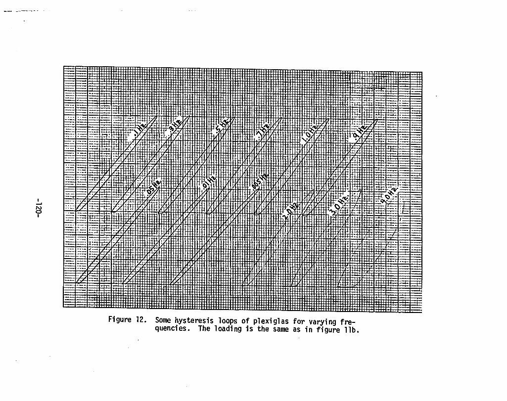
I ..... N o I

1-. iili.' g::::;..

:t:--:--I ..... .·.~I.I .1_

" T-'-'- ;j:t-. ~-t::::::::J ~U; r:.i+; ~b ~-t·~

f=-:r.: . - -tj 'tt:!::!:: -. ., ,. _.ltlmJ:t1! U±t± Itt :1. . lli: il I~~, t=-- :=: ==:: -- .. "- .-. ~ -+·lS-t·~-+<~· ~:f~~-' " fLU~" ~~. ·III-~ If- t .-.- .. fl· ---. , .. --+.,..,-- H+f. ,. . III. v.I" , . • I ~!. I It' ... _"~_ "._. _ -.--4- ' __ _ t= --+i-..... \+ ~~ • • '.. _'--. '~=_ -- - .....--- ... ::r::t - ~" :±' : I '/ . . L ~ - " ... "". ~ t:::::::: ___ _

.. ... '"~ m=::rt t+r+~' i . Itt ?J~ "? ~ • '0.. "~ ~ t=:.: -. - == .' -: I~ '.. _... ".... : .:: • _ • _ - : - . . r I:t!: . .: _._ __ - .. :=: ---I:r"::f. - cr. ,'2, ~; .. ,j,. . ,.~ 'I . . ~ j:!.::f:t: ts::: =_ t-. - '- ·--·l@ rE ~. 1"'1'1 Ift~· , tt '.-_ I---~ -'T . 'I'H, '. " .1.1. '_, _~

- --- -- ......- r' . - -.- • JI~ _ _, r _ _ t::,'._ ------" -tr'+ -~ l:r{f· til,~ .. . . . _ t:t +~ iiI:::, ____ -...:~.=t =-.~ ,r-.(J:: rt' 'J." ,t~il;tt:,: ...............

.. :'- t-. 2.,.1jej:t ~, iLl'" t+: 17·' -,~ 'tt +..; _ r-+-

• - --1'!"h+t- Htt rt,:l ~·H t.4 . li' r:d ~~ 2t:::::::t: tl!J l?:illiit ll2t ~H . t [lU: .·t :: En H Vr • tti

'S __ I_ -=iW· ..::3 ~ ffi1:rnfi1 .• ~t-: ~

I~~-- -~ .. == --- -r - . ,,, .. "' .... r '.t,

~ _. =--:.~, "1T' .-o-rt T

Figure 12. Some hysteresis loops of plexiglas for varying fre­quencies. The loading is the same as in figure 11b.

'-r-t~

I ..... N ..... 1

E. EL EN

a"{t) r"NHI rWNv

a(t:) -Yfl -.

E.

_er(t:) E

~ 4E-'

(a)

E, ~

~I

E=2.144xl09N/m2

El=2.439xl09N/m2 E2=3.467xl010 N/m2 E3=7.724xl010 N/m2 E4=8.440xl010 N/m2

(b)

L.[J ~2. ~N

EL £, E4

~~ "5 ~ ... ~1=1.465xl013 N'sec/m2 ~2=1.141xl013 N'sec/m2 ~3=3.457xlOll N·sec/m2 ~4=3.585xl08 N·sec/m2

cr(t:) ----

Figure 13. The generalized Kelvin-Voigt model used to model a viscoelastic material (a). In figure (b) the actual model and constants used to fit the creep curve for plexiglas (figure 14).

1: '" z: r-

-0 ~ ....

V')- )( ct::J:0"I ..J 00 C!JtJ(\') _If I • ><_(\') LU~II ...J_ 0 Q.tJb

1:: : ., .. .. T' " r !: .. if ..

" . ~ t~:: !!

~~ ::;:: -........ -_. ~

~,.....

~- -- ''';-- ...... -. -......... ~ ......... ~.:~: . ..,.,. ._. ~ ' ... - ..... -

~ :::-t=~tB ". -+-!- ••. 6.

,'!I!, i!:"'::! I .. i" ...

:; ;: ...... ,. io.o ••••

::1: ::::

..... ~~! I : !!! .... , •• 1

:1':: , -:1%: .... . ".

." ., ....... _., t::: :~:; ~:';l :!;t It:: .... :::: z::: :::, .•. ,

:;:: r:r: liil jlti ;;.:;::;.; :i~ ;.:~ ,j,t!i !!;: !:!;::, t~ a~ t:i ::::- :li:j ::r;r -::-:..

::1: ;::.: :::' :l: o r:'::: ......... r .H';'~ it!"! r.::r U~: :~+ :: r: ::!! '" '" "' .•. "'.

"

;: ; .... ~~ [..0.+ ~!;. ~-:H" ,. ~ ~. ..., .•• , ,.. ,'--:! I~. __ ."" ... !"tr ... ". ~-~""""'''I. •• __ .. __ ...... _ ,.. ••. ,,~ , ........

I .. t:::. ~ ... -.,. L:: •• ~ ~.~ ::;t I===I • -- •••• .;:;:;: .-• ! :;~.: ~ ~ ~ ........ _. ::::: =:: ~.;:::.:::: ~

... - -........ -'-.... ~. ..... .- ... -- -- . ., -.~. . --~~r-O- .....,....- ----- ~. -. =: ~:: ::::::; ::...-t ;t::, ::: - == ::::l =-:= •• .; :;z -= ;:::!: • l .......

~ :.: ...... -'!""f ::::::::t '~~ •• _- .. ~~ --- ~~'~ •••••• ~ ;.:;:::- " :: ::::t'~:=:::;= :. _____ ' ~ ......... :: .... __ .........

•• ,~-

---.-.....: .... I.~ ~.~;:::::&O. .

!~ , ...... +-.... I:f;i:;:::=

::'I~~""H - rt:+ • rt" • H' ~"'-H HT 't-'+ ..........

::. ~;.:r;::t ,N't ... t" Mil.... 1~ :11!'"~n' ttl! -:tr: +t!"" tnt t II •. . •. , .•• , 1;.1 rt I ,H, "t .. · , . I ".. ",.. "'; .. " 't, I of I ; rt; tit 11" ., •. I .... ~i· ~ ,,-.. _... -- ~ ...... , ........ .., 1"....... .... ........ ~~ 11111·Lli.i.ii~, "'! tlli~·:!L1.:t!t~~t Ittil tr,:! tl:1 .r.£H ttTrT Tn: :r-l'; tl:! ::1i:L T,t­=11 Fff:f.-H; :j fl4 ::,r;~ .. h:tt It: ' ~r.tt: '';UH+~~ltl'l~m : tr Ull ~tin ;t"t"

I 1111; Ii;!: I:: :l!!;" :;I! ~1I1 [tjl !!i H:J I 'Ill mr1t11! =1'1 lI:l 'It trn' :t' Itit:tlrU! ll. I ..... ..I.' ~.'I .. , ... I .... 11!! , . t, !t. I tit!:

I ' 1111 '1,111:::III::L!·1:::J::P :!I: I::: 1j:1 III :1111111: :1111 II II I I I i II i i j' 'i; i i; II' I ;; I i !ill;; i: : i;; ':.j i U i ij ;; i;f; i ,. : j iii ; 1 ; i . i i Ir

-122-

&II IG .... C) -)( cu .... Co

s.. o

q..

~ s.. ::s u Co cu ~ u

< .

qo .... cu s.. ::s C)

jz.

-' N W I

o o

o o

2.5 o

000 o

000 000 0 0 0 0 0 0 0 000

10 Hz o Experiment

-Theory

ZZ LV __ -L __ -L __ ~ __ ~ __ ~ __ ~ __ ~ __ ~ __ ~~ __ ~ __ ~ __ ~ __ ~ __ ~

5 nxIO'(Gycles)

10

Figure 15. Theoretical and experimental curves for temperature as a function of the number of cycles. The cycling fre­quency ;s 10 hz. The material is plexiglas.

I ..... N

"t

o 0- O-O-O-O-O...,SJ-

T(o,n)c o

o o 0

o

15 Hz

o Experiment

-Theory

Z2LV __ ~~ __ ~ __ ~ ____ ~ __ ~ __ ~ ________ ~ __ ~ ____ ~ __ ~ __ ~~ __ ~ ____ _

10 20 n xl03 (cycles)

Figure 16. Theoretical and'experimental curves for temperature as a function of the number of cycles. The cycling frequency is 15 hz.The material is plexiglas.

-" N til I

----0" ,...-;'--0

2LJ Hz..

o Exp.

Theory

22. r I I I

20 40 60 nx I03(cyc/es)

Figure 17. Theoretical and experimental curves for temperature as a function of the number of cycles. The cycling frequency is 20 hz. The material is plexiglas.

--' N en I

T(o,n)'t

fA)

40

20 n x /03

( cycles)

50Hz.

o Exp. _ Theory

~

Figure 18. Theoretical and experimental curves for temperature as a function of the numbe~ of cycles. The cycling frequency js 50 hz. The material is plexiglas.

ilP,n)c.

40

30

Figure 19.

25Hz.

2DHz.

15Hz

10 Hz

1000 t(.secJ

(a)

25Hz.

20Hz.

151-1z

10Hz

(b) n ( c. yc.le.s )

Theoretical curves of temperature versus time (a) and versus number of cycles (b), for various cycling frequencies.

-127-

References

1. F. De1a1e, F. Erdogan, and M.N. Aydurog1u, "Stresses in adhesively bonded joints: a c10sed-fonn sol ution", Journal of Composite Materials, Vol. 15, pp. 249-271,1981.

2. Y. Weitsman, "An investigation of nonlinear viscoelastic effects on load transfer in a symmetric double-lap joint", Materials Laboratory, Air Force Wright Aeronautical Labora­tories, Wright-Patterson Air Force Base, AFWAL-TR-81-4121, October, 1981.

3. N.I. Muskhe1ishvi1i, Some Basic Problems of the Mathematical Theory of Elasticity, P. Noordhoff, Groninger, Holland, 1953.

4. F. Erdogan, "Ana1ysis of e1asti c cover p1 ates", Developments in Mechanics, Vol. 6, pp. 817-829, 1971.

5. F. Erdogan, "Fracture problems in composite materia1s", Journal of Engineering Fracture Mechanics, Vol. 4, pp. 811-840, 1972.

6. F. Erdogan and M.B. Cive1ek, "Contact problem for an elastic reinforcement bonded to an e1 asti c p1 ate", Journal of App1 ied filechanics, Vol. 41, 'pp. 1014-1018,1974.

7. Hart-Smith, L.J., "Adhesive-bonded single lap joints", Douglas Aircraft Co., ~'cDonnel1 Douglas Corp., Nasa Langley Research Center Contractor Report 112236, January 1973.

8. f1. Go1and and E. Reissner, liThe stresses in cemented joints", Journal of Applied Mechanics, Trans. ASME, Vol. 1, No.1, pp. (A.17)-(A.27), 1944.

9. r·1.L. Hi11iams, N.H. Wackenhut, R.D. Marangoni, N.R. Basavanha11y, E.F.M. Hinter, C.C. Yates, "Mechanica1 spectro­scopy for epoxy resins", Materials Laboratory, Air Force Wright Aeronautical Laboratories, Uri ght-Patterson Ai r Force Base AA~AL-TR-81-4070, August 1981.

10. l~.J. Renten and J.R. Vinson, liThe efficient design of adhe­sive bonded joints",Jouma1 of Adhesion, Vol. 7, pp. 175-193, 1975.

11. F. De1a1e and F. Erdogan, "Viscoe1astic analysis of adhesively bonded joi nts ", Journal of App 1 i ed Mechani cs, Trans. ASME, Vol. 48, pp. 331-338, 1981.

-128-

12. F. Delale and F. Erdogan, "Time-Temperature effect in adhe­sively bonded joints", Journal of Composite r~aterials, V. 15, pp. 561-581, 1981.

13. ~l. Fl ugge, Vi scoe 1 as ti ci ty, Spri nger-Verl ag, 1975.

14. B.A. Boley and J.H. Heiner, Theory of Thermal Stresses, John Wiley and Sons, 1962.

15. and P.G. Klemens, Vol. 2 (1970) and

-129-

Appendix A

Least squares fit to creep data.

The creep curve has the form

E· 1

J(t) 1 t N

=-+-+ I: E A i=l

1 - Ait E:" {l-e ).

1

(Al)

The elastic response of the material is included with the t term in (A1). This value is simply J{O) and can be calculated

directly from the graph (figure 14). The value of A is simply

the inverse slope of the curve for large time. Plexiglas was

assumed to be a solid, therefore A was taken to be infinite. The

remaining constants to be determined in a least squares sense are

Ei' Ai·

Denote the sum of the squares as

E· li:m L N 1 - Ai

R{Ei,Ai) = E [E -E. (l-e ) - D{tm)]2, (A2) m=l i=l 1

where L is the number of data points used and D{tm) are the values

obtained from the curve in figure 14 less the elastic response.

We seek the values of Ei' Ai for a given N that minimizes R. To

do this, we try to solve the following:

k = 1, ••• ,N (A3)

-130-

k = 1, ••• ,N. (A4)

These relations give the following equations

L N E [ E

m=l i=l

E· Ek --'tm --tm

1 Ai tm Ak - (l-e )-D(tm)]{ - e Ei . Ak

E· Ek L E

_ -' t - t N 1 Ai m - Ak '1l1

[E - (l-e )-D(tm)]1;ne =0 m=l i=l Ei

Ek - - t 1 Ak m

- - (l-e )}=o Ek

(A5)

k=l, ••• ,N.

(A6)

Because it is difficult to solve this system of 2N non-

linear equations, the following successive approximation scheme

is used.

First an initial guess was made for the constants. Then El

was determined according to equation (A3). This value replaced the

guessed, initial value of El • Then E2 was determined using (A3).

Again this value replaced the initial value of E2. This procedure

was continued up till N after which Al was determined. It was

found that the sum of the squares decreased after each application

of either equations (A3) or (A4). The iterations were stopped

after the change from one iteration to another was minimal. For

the curve of figure 14,1 used N=4 (see figure 13b).

-131-

Appendix B

In order to obtain more accurate information about the small

time behavior of a creep curve, it is suggested that a ramp load

be applied initially instead of an attempt to experimentally dupli­

cate the unit step function. The loading is ·shown below.

t

and given by the expression

(B-1)

~/ith this as an input we use the Hereditary integral to obtain

the strain.

t e(t) = cr(t)J(O) + J aCt') dJ(t-t') dt'.

d( t-t' ) (B-2)

o

After substituting and integrating we obtain for t < to

-132-

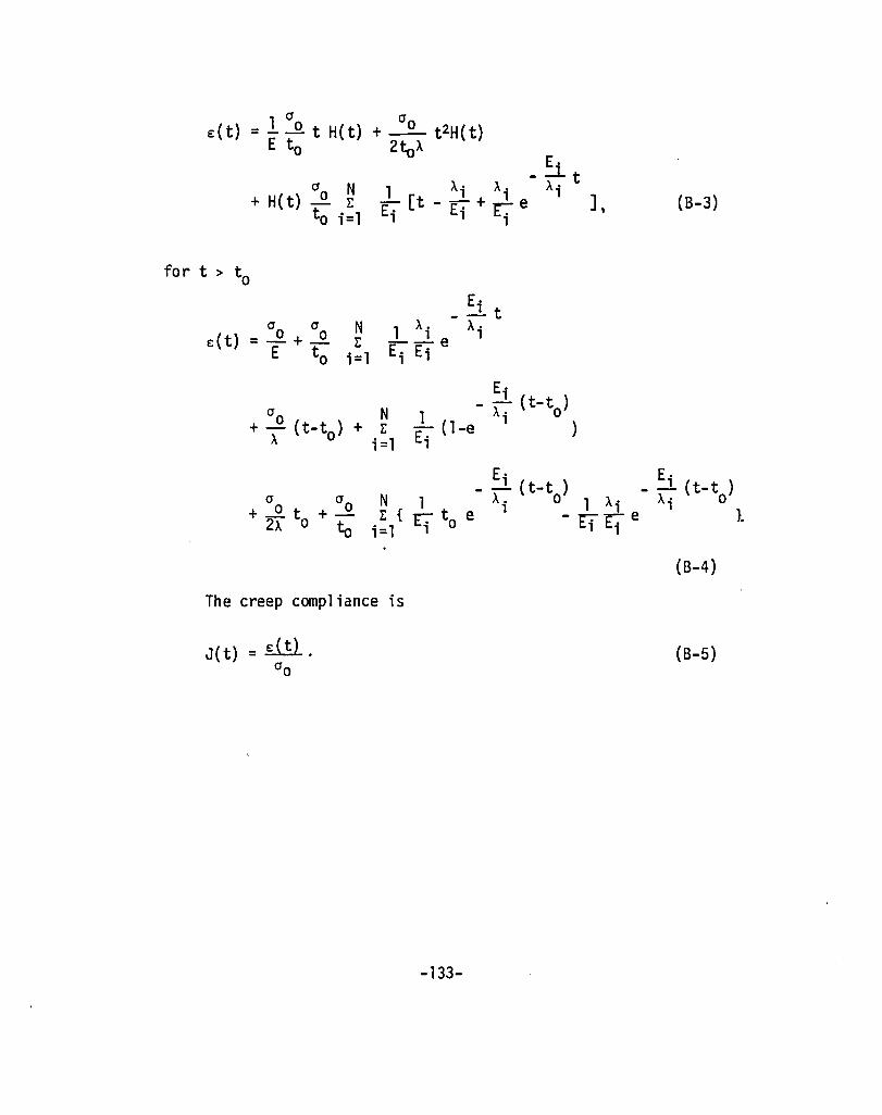
100 E(t) = -~ t H(t) + _____ 0 t 2H(t)

E to 2toA E·

o N + H(t) ~ E

to ;=1

- _1 t 1 A; A; A;

E; [t - E; + r, e

for t > to

o 0 N e:(t) = ~ + ~ E

E to ;=1

E· __ 1 t

1 A. A. __ 1 e 1

E; E;

(B-3)

+ 0 0 t + 0 0

E· E· __ 1 (t-t ) __ 1 (t-t )

N 1 A; 0 1 A; A; 0

2A 0 to E { E"" to e - til· t:1• e 1

i =1 1

(B-4)

The creep compliance ;s

J(t) = iliL. 0 0

(B-5)

-133-

Appendix C

Here the equations of motion are detenmined using an alter­

nate method. Consider a spring and dashpot in parallel and sub­

jected to a load a(t).

The governing equation is

Note here that

for a(t) = d+esinwt we find

eAi w ----coswt. A. 2w2+E·2 . 1 1

Now consider a spring and dashpot in series.

-134-

(C1)

(C2)

(C3)

The governing equation is

Note here that

Sol ving thi s equation for

o(t) = d + e sin wt,

\Ale obtain

() _d e· dee e: t - - + - Sln wt + - t - - cos wt + - . E E A AW AW

(C4 )

( C5)

(C6)

(C7)

Since the spring and dashpot system shown in figure 13a is

linear, simply add (C-7) and each of the N components of (C-3)

to get the identical result obtained from equation (123).

i.e. e:T(t) = e:(t) + ~ e:i(t) i=l

-135-

(C8)

Appendix 0

Solution of the partial differential equation

aT = a a2T + Q- bt at W oe

subject to the conditions (see figure llc)

aT I -° ax x=o -

T(±R., t) = To

T(x,O) = To .

Define ao T(x,s) = f T(x,t)e-stdt

o

c+iao

T(x,t) = J T(x,s)estds.

c-iao

(01)

( 02)

(03)

(04)

(05)

( 06)

After taking the Laplace Transform of (0-1), (0-2) and (0-3),

we obtain

a2f 1 s T(x,s) - T(x,O) = a ~ + Qo s-b (07)

-aT I -° ax x=O

(08)

i(±R., t) (09)

-136-

Rearranging 07 we find

.J ( 010)

which has the solution

T(x,s) = A(s)sinh [f x + B(s)cosh if x

Qo To + +- . s(s-b) S

(011)

After applying the transformed boundary conditions we obtain

T(x,s) = Qo

s(s-b)

cosh fax Qo --~-+ cosh fa ~ s(s-b)

from the inversion integral we can determine T(x,t)i

(012)

c+ioo fS' =

_1_ J { Qo cosh Ja x Qo To st T(x, t) -,...~-:- + --:-~7" + -}e ds 2ni s(s-b) cosh ~ 4- s(s-b) s •

c-ioo /a ~ (013)

Now to calculate the residues. There are contributions from

0, b; and from the zeros of cosh fa~' which occur at

( 014)

The residue at zero is

-137-

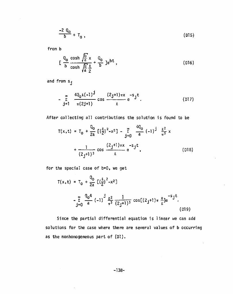
from b

Qo cosh fax Qo bt [- + -]e

b cosh !fj'!. b ' fa 2

and from Sj

co

- I: j=l

4QOi(-1)j (2j+1)~x -s.t ---- cos --- e J . ~(2j+1)

(015)

( 016)

(017)

After collecting all contributions the solution is found to be

Qo i 2 co 4Qo j i 2 T(x,t)=T +-[(~)_X2]- I: -(-1) -x

o 2a ~ j=O a ~3

1 (2j+1)~x -s·t + -~- cos e J J

(2·+1)3 J t

for the special case of b=O, we get

Qo t 2 T(x,t) = To + 2a [(2) _X2]

co Qo4 j i 2 1 -s ·t - I: - (-1) - - cos[(2J'+1)~ ~]e J.

j=O a ~3 (2j+1)3 ~

(018)

( 019)

Since the partial differential equation is linear we can add

solutions for the case where there are several values of: b occurring

as the nonhomogeneous part of (01).

-138-

r 1. Report No.

NASA CR-172124 1 2. Government Accession No. 3. Recipient's Catalog No.

4. Title and Subtitle 5. Report Date

April 1983 VISCOELASTIC STUDY OF AN ADHESIVELY BONDED JOINT 6. Performing Organization Code

7. Author(s) 8. Performing Organization Report No.

Paul F. Joseph 1----------------------------4 10. Work Unit No.

9. Performing Organization Name and Address

Lehigh University Bethlehem, PA 18015

11. Contract or Grant No.

Nt1R 39-007-011 1--_________________________ --113. Type of Report and Period Covered

12. Sponsoring Agency Name and Address

National Aeronautics and Space Administration Washington, DC 20546 U.S. Army Aviation Research and Development Command St. Louis, MO 63166

15. Supplementary Notes

Langley technical monitor: Dr. John H. Crews, Jr.

16. Abstract

Contractor Report 14. Army Project No.

1 L 1611 02AH45

In this study, the plane strain problem of two dissimilar orthotropic plates bonded with an isotropic, linearly viscoelastic adhesive was considered. Both the shear and the normal stresses in the adhesive were calculated for various geometries and loadings. Transverse shear deformations of the adherends were included, and their effect is shown in the results. All three in-plane strains of the adhesive were included. Attentionwas given to the effect of temperature, both in the adhe­sive joint problem in Part I and in a separate study of heat generation in a viscoelastic material under cyclic loading in Part II.

In Part I, if the temperature is taken as a known piecewise constant function of time, the differential equations have constant coefficients and the Laplace Transform technique can be directly applied. In the heat generation problem, the one-dimensional coupled heat equation is solved. It is shown that the coupling term is negligible. Both experimental and theoretical results are given for vari­ous cycling frequencies.

An extension of the joint problem in Part I is a calculation of the strain energy release rate when debonding occurs. The fracture energy was found to be nearly independent of the bond length for lengths consistent with a plate theory.

17. Key Words (Suggested by Author (s))

Adhesive bonding Orthotropic plates Viscoelasticity Heat generation Temperature .. :",~;"talrp pnprov

19. Security Classif. (of this report)

Unclassified .

18. Distribution Statement

Unclassified - Unlimited

20. Security Classif. (of this page)

Unclassified 21. No. of Pages

139

Subject Category 39

22. Price"

A07

For sale by the National Technical Information Service, Springfield, Virginia 22161

End of Document