OPTICAL MICROSCOPE

1

THE LIGHT MICROSCOPE v THE ELECTRON MICROSCOPE

fluorescent (TV) screen,photographic film

Human eye (retina), photographic film

Focussing screen

VacuumAir-filledInteriorMagnetsGlassLenses

High voltage (50kV) tungsten lamp

Tungsten or quartz halogen lamp

Radiation source

x500 000x1000 – x1500Maximum magnification

0.2nmFine detail

app. 200nmMaximum resolving power

Electronsapp. 4nm

Monochrome

Visible light760nm (red) – 390nm

Colours visible

Electromagnetic spectrum used

ELECTRON MICROSCOPELIGHT MICROSCOPEFEATURE

© 2007 Paul Billiet ODWS2

THE LIGHT MICROSCOPE v THE ELECTRON MICROSCOPE

Copper gridGlass slideSupport

Heavy metalsWater soluble dyesStains

Microtome only.Slices 50nm

Parts of cells visible

Hand or microtomeslices 20 000nmWhole cells visible

SectioningResinWaxEmbedding

OsO4 or KMnO4AlcoholFixation

Tissues must be dehydrated

= dead

Temporary mounts living or dead

Preparation of specimens

ELECTRON MICROSCOPELIGHT MICROSCOPEFEATURE

© 2007 Paul Billiet ODWS 3

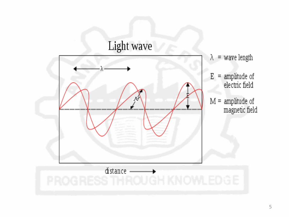
What is a Light?• Light is electromagnetic radiation that is visible to

the human eye, and is responsible for the sense of sight.

• Visible light has a wavelength in the range of about 380 nm to about 740 nm – between the invisible infrared, with longer wavelengths and the invisible ultraviolet, with shorter wavelengths.

• Primary properties of visible light are – Intensity, – Propagation direction,  – Frequency or wavelength spectrum– Polarisation

• Light rays are usually perpendicular to wave front

4

5

UNITS OF MEASUREMENT1m = 103 mm (millimetres)1m = 106 µm (micrometres)1m = 109 nm (nanometres)

Sometimes in old texts Angstroms (Å) are used (the diameter of a hydrogen atom)

1m = 1010 Å

6

The electromagnetic spectrum

7

8

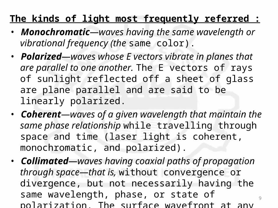
The kinds of light most frequently referred :• Monochromatic—waves having the same

wavelength or vibrational frequency (the same color).

• Polarized—waves whose E vectors vibrate in planes that are parallel to one another. The E vectors of rays of sunlight reflected off a sheet of glass are plane parallel and are said to be linearly polarized.

• Coherent—waves of a given wavelength that maintain the same phase relationship while travelling through space and time (laser light is coherent, monochromatic, and polarized).

• Collimated—waves having coaxial paths of propagation through space—that is, without convergence or divergence, but not necessarily having the same wavelength, phase, or state of polarization. The surface wavefront at any point along a cross-section of a beam of collimated light is planar and perpendicular to the axis of propagation.

9

10

11

12

13

14

15

IMAGE FORMATION

16

IMAGE FORMATION• A specimen is placed at a position A

where it is between one and two focal length from an objective lens.

• Light rays from the object firstly converge at the objective lens and are then focused at position B to form a magnified inverted image.

• The light rays from the image are further converged by the second lens (projector lens) to form a final magnified image of an object at C.

17

MAGNIFICATION• The magnification of a microscope

can be calculated by linear optics.

•f is the focal length of the lens •v is the distance between the image and lens

• A Higher magnification lens has a shorter focal length.

18

• The two lenses are called:– Eyepiece– Objective

• The eyepiece has a magnification of “10x”• The magnification of the objective lenses

vary and are marked on the lens• Total magnification =

(Eyepiece) X (Objective)• Example:

10 X 40 =

Magnification

40019

The Parts of the Microscope and Their Function

Magnification

Support body tube

Supports slide

Focuses image

Sharpens the image

Supports microscope

Reflects lighttowards eyepiece

Regulatesamount of light

Holds slide In place

Hold objectives-rotates to changemagnification

Magnification

Maintainsproper distancebetween lenses

20

Storing the Microscope

1. the 10X objective is in place

2. the stage is all the way down

3. the power is off 4. the cord is

wrapped around the base

Four steps prepare the microscope for storage:

21

Eyepiece

Arm

Stage

Course adjustment

Fine adjustment

Base

Let’s Review!

12.

13.

9.

10.

11.

14.

Body tube

Nosepiece

Low power

High power

Stage clips

Diaphragm

Light source

Medium power

1.

2.

3.

4.

5.

6.

7.

8.

22

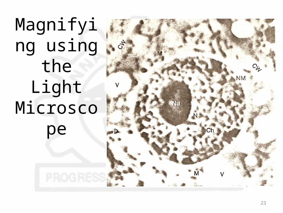
Magnifying using

the Light Microscop

e

23

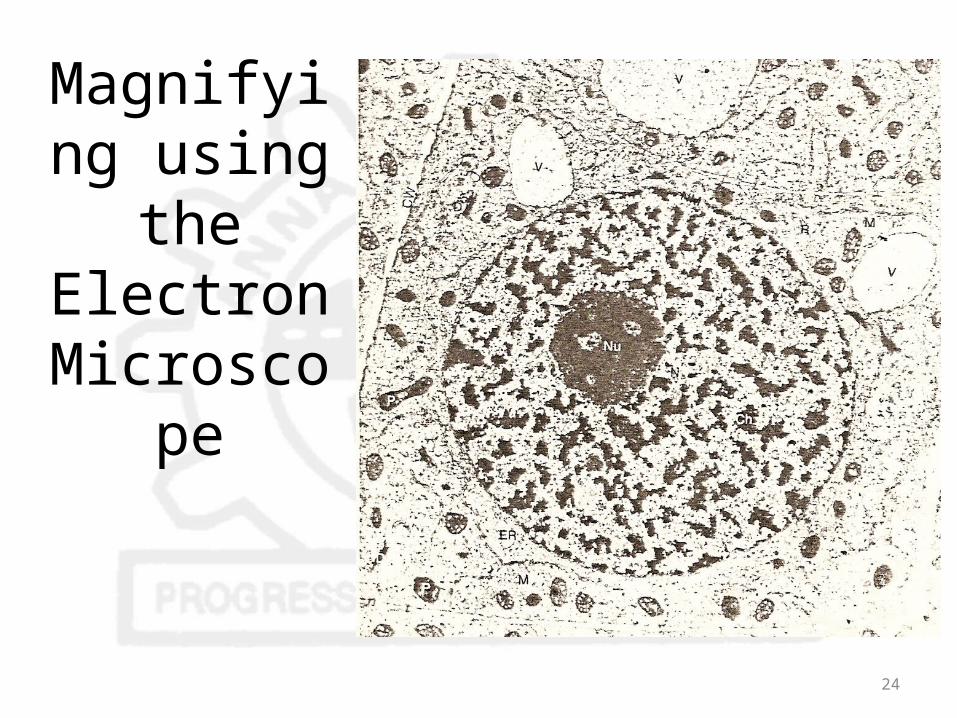
Magnifying using

the Electron Microsco

pe

24

MAKE A SIMPLE MICROSCOPE• You can make a simple microscope by using

magnifying glasses and paper:• Get two magnifying glasses and a sheet of printed

paper.• Hold one magnifying glass a short distance above

the paper. The image of the print will look a little bit larger.

• Place the second magnifying glass between your eye and the first magnifying glass.

• Move the second glass up or down until the print comes into sharp focus. You will notice that the print appears larger than it does in the first magnifying glass.

25

Resolution• Resolution refers to the

minimum distance between two points at which they can be visibly distinguished as two points.

• Whenever light passes through an aperture, diffraction occurs so that parallel beam of light is transformed into a series of cone, which are seen as circle and they are know as Airy ring.

• The resolution of a microscope (R) is defined as the minimum distance between two Airy disks that can be distinguished

26

Resolution• Resolution is a function of microscope parameters.• Where μ is the refractive index of the medium between the object and objective

lens and α is the half-angle of the cone of light entering the objective lens. • The product μsin α, is called the numerical aperture (NA).• To achieve higher resolution we should use shorter wavelength light and larger

NA.

27

Effective Magnification• Magnification is meaningful only in so far as the

human eye can see the features resolved by the microscope.

• Meaningful magnification is the magnification that is sufficient to allow the eyes to see the microscopic features resolved by the microscope.

• A microscope should enlarge features to about 0.2 mm, the resolution level of the human eye.

• Thus, the effective magnification of light microscope should approximately be Meff =0.2/0.2×103 = 1.0×103.

28

Brightness and Contrast• To make a microscale object in a material

specimen visible, high magnification is not sufficient.

• A microscope should also generate sufficient brightness and contrast of light from the object.

• Brightness refers to the intensity of light.– In a transmission light microscope the

brightness is related to the numerical aperture (NA) and magnification (M).

29

– In a reflected light microscope the brightness is more highly dependent on NA.

• These relationships indicate that the brightness decreases rapidly with increasing magnification, and controlling NA is not only important for resolution but also for brightness, particularly in a reflected light microscope.– Contrast is defined as the relative change in light intensity (I) between an object and its background.

30

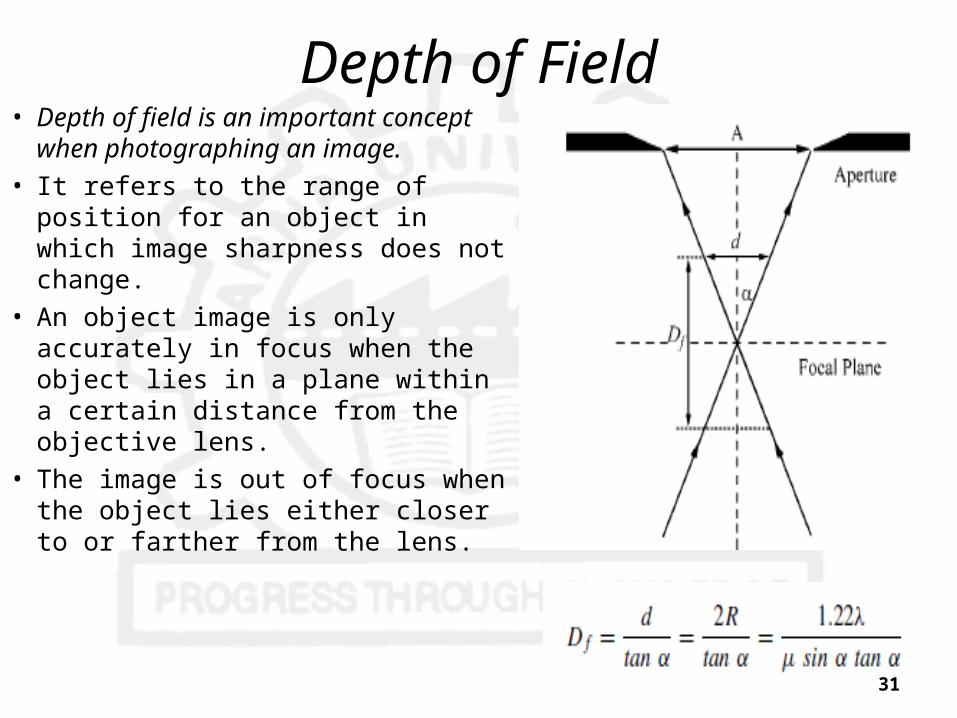
Depth of Field• Depth of field is an important

concept when photographing an image.

• It refers to the range of position for an object in which image sharpness does not change.

• An object image is only accurately in focus when the object lies in a plane within a certain distance from the objective lens.

• The image is out of focus when the object lies either closer to or farther from the lens.

31

Depth of Focus• We should not confuse depth of field with depth

of focus.• Depth of focus refers to the range of image

plane positions at which the image can be viewed without appearing out of focus for a fixed position of the object.

• In other words, it is the range of screen positions in which and images can be projected in focus.

• The depth of focus is M2 times larger than the depth of field.

32

Aberrations• The aforementioned calculations of resolution and

depth of field are based on the assumptions that all components of the microscope are perfect, and that light rays from any point on an object focus on a correspondingly unique point in the image.

• Unfortunately, this is almost impossible due to image distortions by the lens called lens aberrations.– Some aberrations affect the whole field of the

image called chromatic and spherical aberrations.– while others affect only off-axis points of the image

called astigmatism and curvature of field.

33

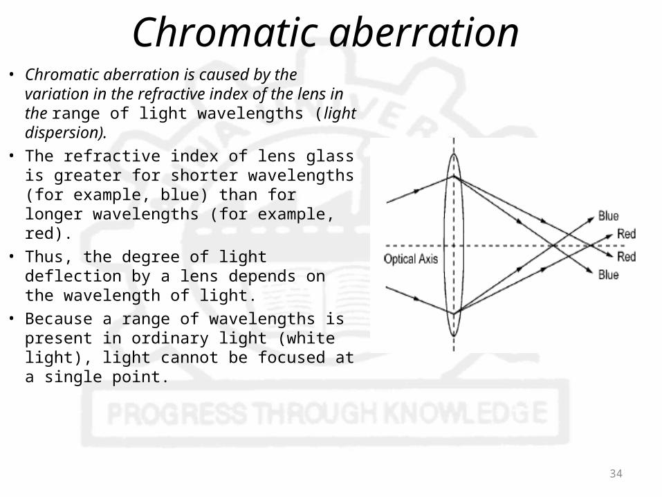
Chromatic aberration• Chromatic aberration is caused by the

variation in the refractive index of the lens in the range of light wavelengths (light dispersion).

• The refractive index of lens glass is greater for shorter wavelengths (for example, blue) than for longer wavelengths (for example, red).

• Thus, the degree of light deflection by a lens depends on the wavelength of light.

• Because a range of wavelengths is present in ordinary light (white light), light cannot be focused at a single point.

34

Spherical aberration• Spherical aberration is caused

by the spherical curvature of a lens.

• Light rays from a point on the object on the optical axis enter a lens at different angles and cannot be focused at a single point.

• The portion of the lens farthest from the optical axis brings the rays to a focus nearer the lens than does the central portion of the lens.

35

Astigmatism• Astigmatism results when the

rays passing through vertical diameters of the lens are not focused on the same image plane as rays passing through horizontal diameters.

• In this case, the image of a point becomes an elliptical streak at either side of the best focal plane.

• Astigmatism can be severe in a lens with asymmetric curvature.

36

Curvature of field• Curvature of field is an off-

axis aberration.• It occurs because the focal

plane of an image is not flat but has a concave spherical surface.

• This aberration is especially troublesome with a high magnification lens with a short focal length.

• It may cause unsatisfactory photography.

37

Instrumentation• Light microscope includes the

following main components:– Illumination system;– Objective lens;– Eyepiece;– Photomicrographic system; and– Specimen stage.

38

Illumination System• The illumination system of a

microscope provides visible light by which the specimen is observed.– Low-voltage tungsten filament bulbs;– Tungsten–halogen bulbs; and– Gas discharge tubes.

39

Objective Lens and Eyepiece

• The objective lens generates the primary image of the specimen, and its resolution determines the final resolution of the image.

• Classification of the objective lens is based on its aberration correction capabilities– Achromat

• The achromatic lens corrects chromatic aberration for two wavelengths (red and blue). It requires green illumination to achieve satisfactory results for visual observation and black and white photography.

– Semi-achromat (also called ‘fluorite’)• The semi-achromatic lens improves correction of chromatic aberration.

Its NA is larger than that of an achromatic lens with the same magnification and produces a brighter image and higher resolution of detail.

– Apochromat.• The apochromatic lens provides the highest degree of aberration

correction. It almost completely eliminates chromatic aberration. It also provides correction of spherical aberration for two colors. Its NA is even larger than that of a semi-achromatic lens.

40

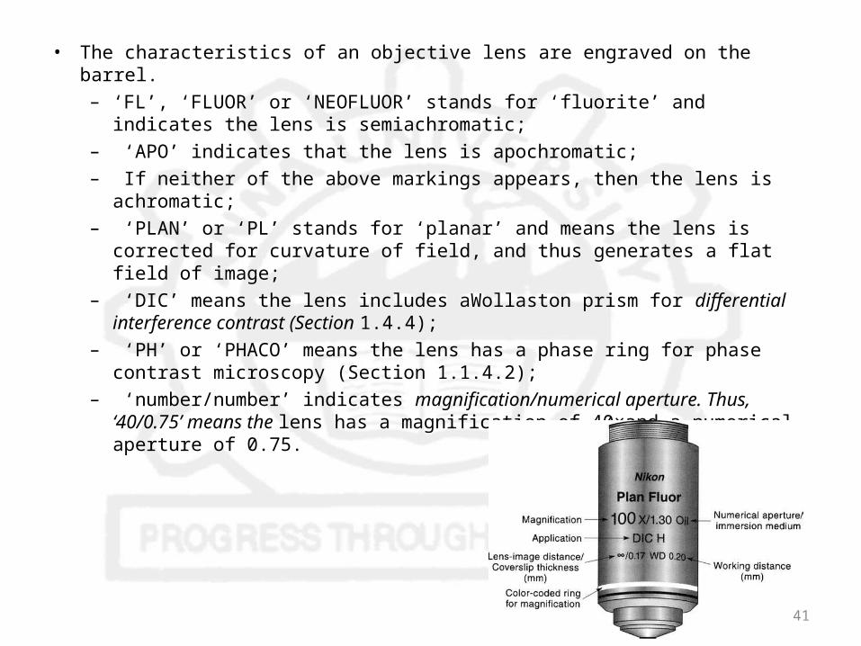
• The characteristics of an objective lens are engraved on the barrel.– ‘FL’, ‘FLUOR’ or ‘NEOFLUOR’ stands for ‘fluorite’ and indicates

the lens is semiachromatic;– ‘APO’ indicates that the lens is apochromatic;– If neither of the above markings appears, then the lens is

achromatic;– ‘PLAN’ or ‘PL’ stands for ‘planar’ and means the lens is corrected

for curvature of field, and thus generates a flat field of image;– ‘DIC’ means the lens includes aWollaston prism for differential

interference contrast (Section 1.4.4);– ‘PH’ or ‘PHACO’ means the lens has a phase ring for phase

contrast microscopy (Section 1.1.4.2); – ‘number/number’ indicates magnification/numerical aperture.

Thus, ‘40/0.75’ means the lens has a magnification of 40×and a numerical aperture of 0.75.

41

Steps for Optimum Resolution

• Use an objective lens with the highest NA possible;• Use high magnification;• Use an eyepiece compatible with the chosen

objective lens;• Use the shortest possible wavelength light;• Keep the light system properly centered;• Use oil immersion lenses if available;• Adjust the field diaphragm for maximum contrast

and the aperture diaphragm for maximum resolution and contrast;

• Adjust brightness for best resolution.

42

Steps to Improve Depth of Field

• Reduce NA by closing the aperture diaphragm, or use an objective lens with lower NA;

• Lower the magnification for a given NA;• Use a high-power eyepiece with a low-

power, high-NA objective lens; and• Use the longest possible wavelength light.

43

Specimen Preparation• The microstructure of a material can only

be viewed in a light microscope after a specimen has been properly prepared.

• The main steps of specimen preparation for light microscopy include the following.– Sectioning– Mounting– Grinding– Polishing– Etching

44

Sectioning• Sectioning serves two purposes:

– generating a cross-section of the specimen to be examined;

– reducing the size of a specimen to be placed on a stage of light microscope, or reducing size of specimen to be embedded in mounting media for further preparation processes.

• Cutting

45

Microtomy• Microtomy refers to sectioning materials with a

knife. It is a common technique in biological specimen preparation.

• It is also used to prepare soft materials such as polymers and soft metals.

• Tool steel, tungsten carbide, glass and diamond are used as knife materials.

• A similar technique, ultramicrotomy, is widely used for the preparation of biological and polymer specimens in transmission electron microscopy.

46

Mounting• Mounting refers to embedding specimens in mounting

materials (commonly thermosetting polymers) to give them a regular shape for further processing.

• Mounting is not necessary for bulky specimens, but it is required for specimens that are too small or oddly shaped to be handled or when the edge of a specimen needs to be examined in transverse section.

• Mounting is popular now because most automatic grinding and polishing machines require specimens to have a cylindrical shape.

• There are two main types of mounting techniques: – hot mounting – cold mounting.

47

Hot Mounting• Hot mounting uses hot-press

equipment as shown in Figure.• A specimen is placed in the

cylinder of a press and embedded in polymeric powder.

• The surface to be examined faces the bottom of the cylinder. Then, the specimen and powder are heated at about 150 ◦C under constant pressure for tens of minutes.

• Heat and pressure enable the powder to bond with the specimen to form a cylinder.

48

Cold Mounting • In cold mounting, a polymer resin, commonly

epoxy, is used to cast a mold with the specimen at ambient temperature.

• A typical mold and specimens for cold mounting is explained in the figure.

• A cold mounting medium has two constituents: a fluid resin and a powder hardener.

• The resin and hardener should be carefully mixed in correct proportion.

• Curing times for mounting materials vary from tens of minutes to several hours, depending on the resin type.

49

• Cold mounting of specimens:

• (a) place specimens on the bottom of molds supported by clamps

• (b) cast resin into the mold.

50

• Cold mounted specimens:• (a) mounted with

polyester

• (b) mounted with acrylic

• (c) mounted with acrylic and mineral fillers.

51

Grinding• Grinding refers to flattening the surface to be

examined and removing any damage caused by sectioning.

• The specimen surface to be examined is abraded using a graded sequence of abrasives, starting with a coarse grit.

• Abrasive paper is graded according to particle size of abrasives such as 120-, 240-, 320-, 400- and 600-grit paper.

• Running water is supplied to cool specimen surfaces during hand grinding.

52

Polishing• Polishing is the last step in producing a flat, scratch-

free surface.• After being ground to a 600-grit finish, the specimen

should be further polished to remove all visible scratches from grinding.

• Polishing generates a mirror-like finish on the specimen surface to be examined.

• Polishing is commonly conducted by placing the specimen surface against a rotating wheel either by hand or by a motor-driven specimen holder.

• Coarse polishing uses abrasives with a grit size in the range from 3 to 30μm.

53

Etching• Chemical etching is a method to

generate contrast between microstructural features in specimen surfaces.

• Etching is a controlled corrosion process by electrolytic action between surface areas with differences in electrochemical potential.

• During etching, chemicals (etchants) selectively dissolve areas of the specimen surface because of the differences in the electrochemical potential by electrolytic action between surface areas that exhibit differences.

54

Polarization Technique• Light, as an electromagnetic wave, vibrates

in all directions perpendicular to the direction of propagation.

• If light waves pass through a polarizing filter, called a polarizer, the transmitted wave will vibrate in a single plane. Such light is referred to as plane polarized light.

55

56

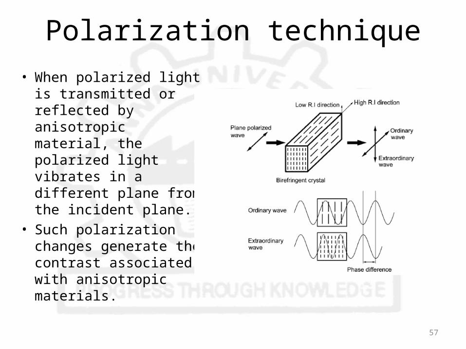
Polarization technique• When polarized light

is transmitted or reflected by anisotropic material, the polarized light vibrates in a different plane from the incident plane.

• Such polarization changes generate the contrast associated with anisotropic materials.

57

• For a transparent crystal, the optical anisotropy is called double refraction, or birefringence, because refractive indices are different in two perpendicular directions of the crystal.

• polarized light ray hits a birefringent crystal, the light ray is split into two polarized light waves (ordinary wave and extraordinary wave) vibrating in two planes perpendicular to each other.

• Because there are two refractive indices, the two split light rays travel at different velocities, and thus exhibit phase difference.

• If the two polarized-light waves have a phase difference of λ/4 , the projection of resultant light is a spiraling circle. 58

59

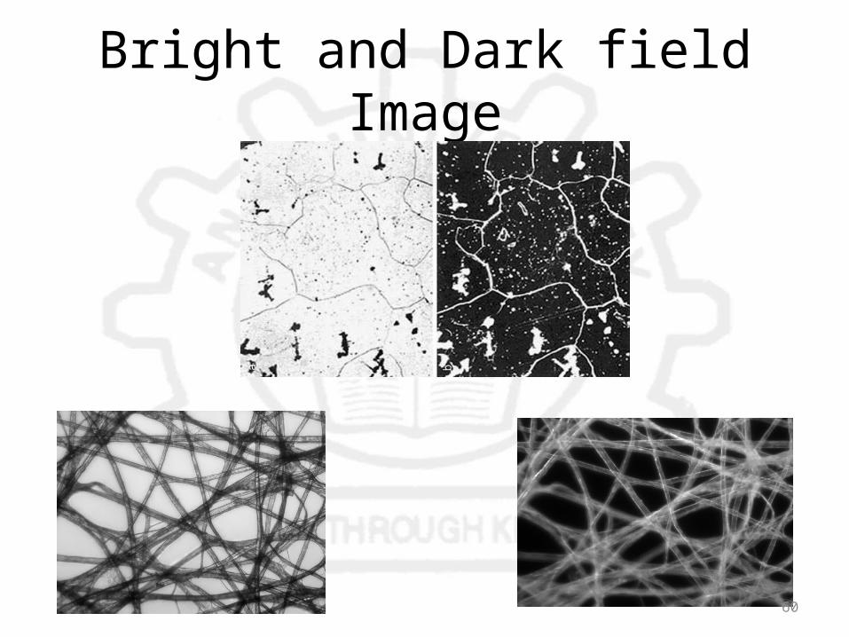
Bright and Dark field Image

60

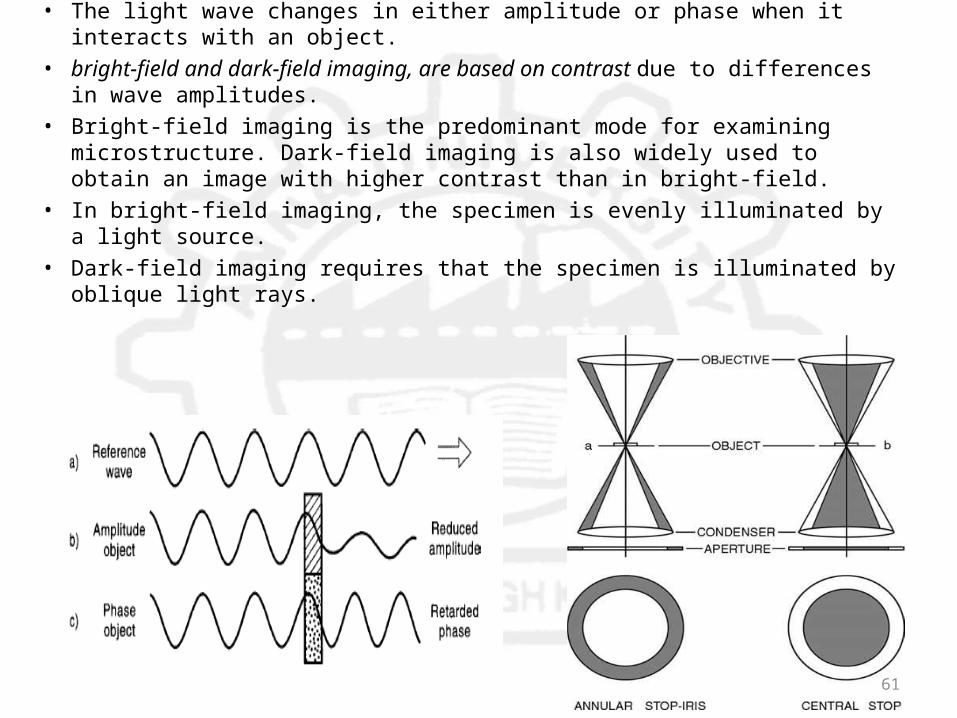
• The light wave changes in either amplitude or phase when it interacts with an object.

• bright-field and dark-field imaging, are based on contrast due to differences in wave amplitudes.

• Bright-field imaging is the predominant mode for examining microstructure. Dark-field imaging is also widely used to obtain an image with higher contrast than in bright-field.

• In bright-field imaging, the specimen is evenly illuminated by a light source.

• Dark-field imaging requires that the specimen is illuminated by oblique light rays.

61

Bright field Images• The light path of a bright field microscope is

extremely simple, no additional components are required beyond the normal light microscope setup.

• The light path therefore consists of: Transillumination light source, commonly a halogen lamp in the microscope stand.

• Condenser lens which focusses light from the light source onto the sample.

• Objective lens which collects light from the sample and magnifies the image.

• Oculars and/or a camera to view the sample image.

62

Dark field Image• Light enters the microscope for

illumination of the sample.• A specially sized disc, the patch

stop (see figure) blocks some light from the light source, leaving an outer ring of illumination. A wide phase annulus can also be reasonably substituted at low magnification.

• The condenser lens focuses the light towards the sample.

• The light enters the sample. Most is directly transmitted, while some is scattered from the sample.

• The scattered light enters the objective lens, while the directly transmitted light simply misses the lens and is not collected due to a direct illumination block (see figure).

• Only the scattered light goes on to produce the image, while the directly transmitted light is omitted.

63

Quantitative metallography• Quantitative metallography is often used to confirm the proper

processing of metallic materials.• Measurements include determination of the volume fraction of a phase

or constituent, measurement of the grain size in polycrystalline metals and alloys, measurement of the size and size distribution of particles, assessment of the shape of particles, and spacing between particles.

• Standards organizations, including ASTM International's Committee E-4 on Metallography and some other national and international organizations, have developed standard test methods describing how to characterize microstructure quantitatively.

• For example, the amount of a phase or constituent, that is, its volume fraction, is defined in ASTM E 562; manual grain size measurements are described in ASTM E 112 (equiaxed grain structures with a single size distribution) and E 1182 (specimens with a bi-modal grain size distribution)

64

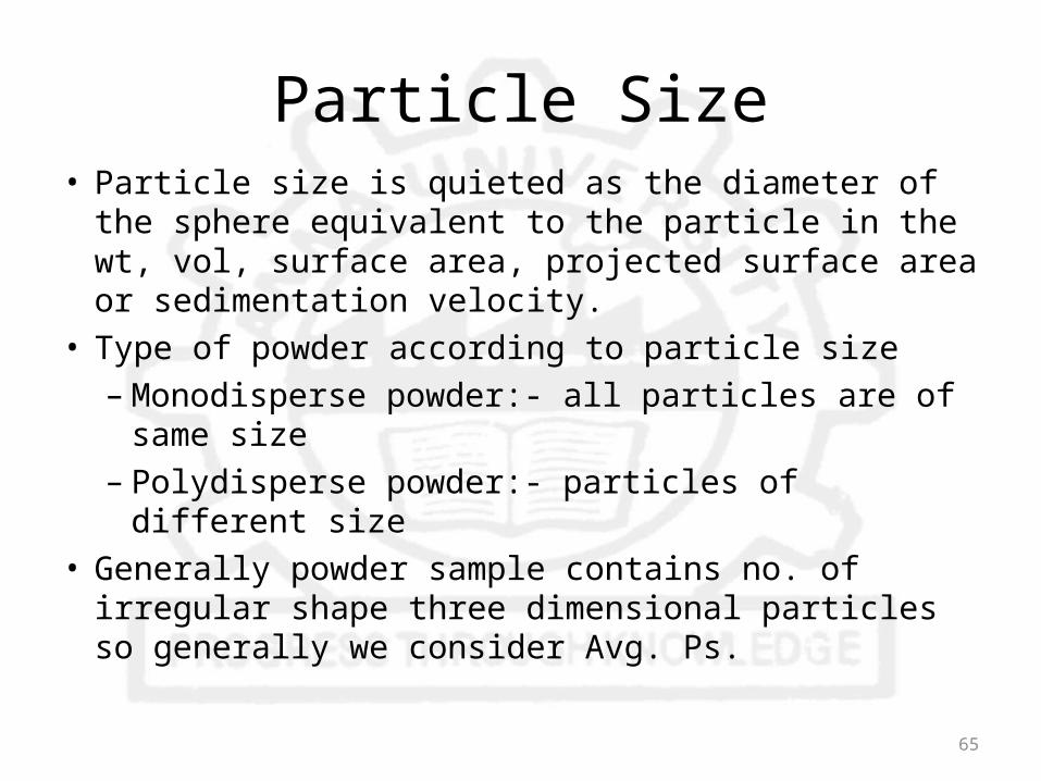
Particle Size• Particle size is quieted as the diameter of the

sphere equivalent to the particle in the wt, vol, surface area, projected surface area or sedimentation velocity.

• Type of powder according to particle size– Monodisperse powder:- all particles are of

same size– Polydisperse powder:- particles of different size

• Generally powder sample contains no. of irregular shape three dimensional particles so generally we consider Avg. Ps.

65

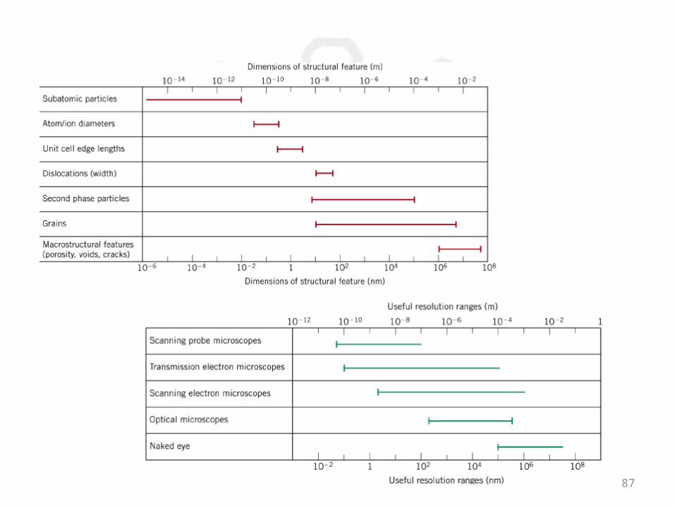
What ranges do we need to measure

• Particle Characterization: Light Scattering Methods66

Principles for different methods

• Visual methods (e.g., optical, electron, and scanning electron microscopy combined with image analysis)

• Separation methods (e.g., sieving, classification, impaction, chromatography)

• Stream scanning methods (e.g., electrical resistance zone, and optical sensing zone measurements)

• Field scanning methods (e.g., laser diffraction, acoustic attenuation, photon correlation spectroscopy)

• Sedimentation• Surface methods (e.g., permeability, adsorption)

67

68

Benefits– “Simple” and intuitive– Give shape information– Reasonable amount of

sample

• Drawbacks– Statistic relevance

“tedious” if image analyse can not be used

– Risk for bias interpretation– Difficult for high

concentrations– Sample preparation might

be difficult

Visual methodsMicroscopy

Principe of operation– Optic or electronic

measures – Two dimensional projection

• Projection screen or circles

• Image analysing programs

• Measures– Feret diameters – Equal circles

• Size range- 0.001-1000 m• Gives number average,or area

average

69

VisualDifferent types of

microscope• Light microscope (1-1000 m)• Fluorescence microscope• Confocal laser scanning microscopy• Electron microscope

– SEM (0.05-500 m)– TEM (Å-0.1 m)

70

Separation methods Sieving

• Principe of operation – stack of sieves that are

mechanical vibration for pre-decided time and speed

– Air-jet sieving - individual sieves with an under pressure and air stream under the sieve which blows away oversize particles

• Measures - Projected perimeter-square, circle– Size range - 5-125 000 m

• Gives weight average

Benefits– “Simple” and intuitive– Works well for larger

particles

Drawbacks– Can break up weak

agglomerates (granulates)

– Does not give shape information

– Need substantial amount of material

– Needs calibration now and then

71

Separation methods

Powder grades according to BP Description Sieve diameter m Sieve that do not

allow more than 40% to pass m

Coarse 1700 355

Moderate coarse 710 250

Moderate fine 355 180

Fine 180

Very fine 12572

Separation methodsChromatography

• Measures– Hydrodynamic radius

• Principel of operation – Size exclusion (SEC

GPC): • porous gel beads• Size range -0.001-0.5 m

– Hydrodynamic Chromatography (HDC)

• Flow in narrow space• Size range capillary -

0.02-50 m packed column 0,03-2 m

• Benefits– Short retention times– Separation of different

fractions• Drawbacks

– Risk for interaction– Need detector

73

Separation methodsFFF (Field flow fractionation)

• Size range 30nm- 1m

• Principe of operation – Flow in a channel

effected by an external field• Heat• Sedimentation• Hydraulic• Electric field

• Benefits– No material

interaction– High resolution– Good for large

polymers• Drawbacks

– Few commercial instrument

– Still in development stage

74

Separation methods Cascade impactores

• Measure- Aerodynamic volume,

• Principe of operation– The ability for particles

to flow an air flow• Size range normally 1-10

m

• Benefits– Clear relevance for

inhalation application– Can analyse content

of particles• Drawbacks

– Particles can bounce of the impactor or interact by neighbouring plates

– Difficult to de-aggregate particles

75

Stream Scanning MethodsCoulter counter

• Measures - Volume diameter• Gives number or mass

average– Size range - 0.1-2000 m– Principe of operation

Measurement on a suspension that is flowing through a tube, when a particle passes through a small hole in a sapphire crystal and the presence of a particle in the hole causes change in electric resistance

• Benefits – measure both mass

and population distributions accurately

Drawbacks • Risk for blockage by

large particles,– More than one particle

in sensing zone– Particles need to

suspended in solution

76

Methods to measure particle size

Light scattering• Measures - Area diameter

or volume diameter, polymers Radius of gyration or molecular mass

• Principal of operation– Interaction with laser

light the light are scattered and the intensity of the scattered light are measured

– Two principals• Static light scattering• Dynamic light

scattering– Size range- 0.0001-1000

m

• Benefits – Well established– instruments are easy to

operate – yield highly reproducible

dataDrawbacks

• Diluted samples-changes in properties

• Tendency to– Oversize the large

particles– Over estimates the

number of small particles

77

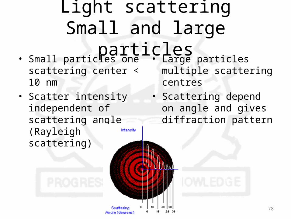
Light scatteringSmall and large particles

• Small particles one scattering center < 10 nm

• Scatter intensity independent of scattering angle (Rayleigh scattering)

• Large particles multiple scattering centres

• Scattering depend on angle and gives diffraction pattern

QuickTime™ and a decompressorare needed to see this picture.78

Sedimentation• Measures - Frictional

drag diameter, stoke diameter

• Gives weight average– Principe of operation

• Sedimentation in gravitational field

• Sedimentation due to centrifugal force

– Size range -0.05-100 gm)

Benefits– “Simple” and intuitive– Well established

Drawbacks• Sensitive to temperature

due to density of media• Sensitive to density

difference of particles• Orientation of particles to

maximize drag• bias in the size distribution

toward larger particle

v 2d2g

18

79

Grain Size Measurements

• Grain structure is usually specified by giving the average diameter.

• Grain size can be measured by two methods.

• (a) Lineal Intercept Technique: This is very easy and may be the preferred method for measuring grain size.

• (b) ASTM Procedure: This method of measuring grain size

• is common in engineering applications.80

TYPES DISTRIBUTIONS

81

Lineal Intercept Technique

• In this technique, lines are drawn in the photomicrograph, and the number of grain-boundary intercepts, N1, along a line is counted.

• • The mean lineal intercept is then given as:

• where L is the length of the line and M is the magnification

• in the photomicrograph of the material.

82

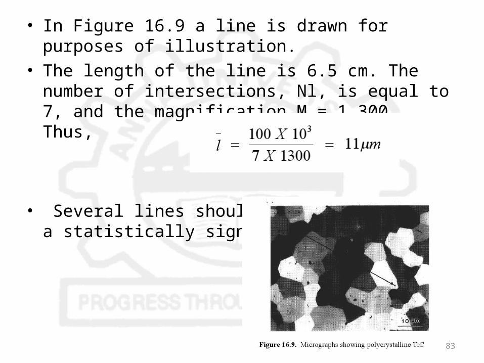
• In Figure 16.9 a line is drawn for purposes of illustration.

• The length of the line is 6.5 cm. The number of intersections, Nl, is equal to 7, and the magnification M = 1,300. Thus,

• Several lines should be drawn to obtain a statistically significant result.

83

• The mean lineal intercept l does not really provide the grain size, but is related to a fundamental size parameter, the grain-boundary area per unit volume, Sv, by the equation

• The most correct way to express the grain size (D) from lineal intercept measurements is:

• Therefore, the grain size (D) of the material of Figure 10.4 Is:

84

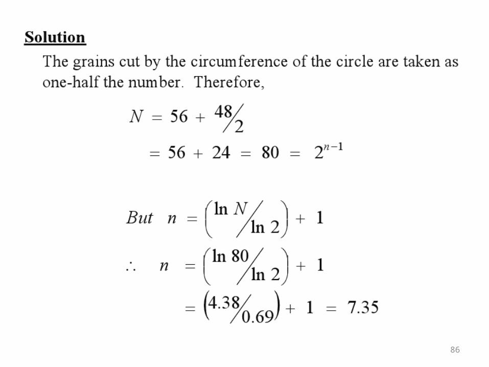
ASTM Procedure• With the ASTM method, the grain size is specified by

the number n in the expression N = 2 n-1

• where N is the number of grains per square inch (in an area of 1 in2), when the sample is examined at 100 power micrograph.

• Example : In a grain size measurement of an aluminum sample, it was found that there were 56 full grains in the area, and 48 grains were cut by the circumference of the circle of area 1 in2. Calculate ASTM grain size number n for this sample.

85

86

87

ASTM Grain size number• ASTM has prepared several standard comparison

charts, all having different average grain sizes. • To each is assigned a number from 1 to 10, which is

termed the grain size number; the larger this number, the smaller the grains.

• It is now common to express grain sizes in terms of a simple exponential equation: – n = 2 G – 1

– where: n (N)= the number of grains per square inch at 100X magnification, and G (n)= the ASTM grain size number.

88

Common methods to estimate the Grain size

• Comparison method– The overall appearance of the microstructure is simply

compared with a standard set of micrographs or plates for which the ASTM Grain size number is determined.

• Grain Counting Method– The number of grains per unit area is counted directly.

The ASTM grain size is then determined according to the definition.

• Intercept Methods– The number of grain boundary intercept per unit test

line is measured. This is a measure of grain boundary area per unit volume and is, therefore related to the grain size

89

Comparison Methods• This is simplest yet least quantitative method and is

described ASTM E122(section 8). • Because the comparison of grain structure may be

influenced by overall type of microstructure. Four standard categories of grain size plates are used for comparision

90

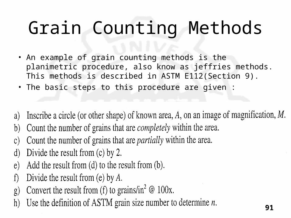
Grain Counting Methods• An example of grain counting methods is the

planimetric procedure, also know as jeffries methods. This methods is described in ASTM E112(Section 9).

• The basic steps to this procedure are given :

91

Intercept Methods• An example of an intercept methods is the linear

intercept procedure, also know as the heyn method. This described in ASTM E112(Section 11) standard.

92

Microstructure of Engineering Materials

• Microstructure of an engineering material is a result of its chemical composition and processing history . It also determine chemical, physical and mechanical property.

• Microstructure influences virtually all aspects of the behavior of materials.

• Macrostructure is the spatial distribution of material in the useful object that is the goal of the endeavor.

93

Procedure• n100 = Nm * [M / 100]2

– n100 : number of grains per square inch at 100x magnification.

– Nm : number of grains per square inch at the magnification M of the photomicrograph.

• N100= 2N-1

• The ASTM grain size number N= [ ln (N100 ) / ln ( 2) ] + 1

• How to calculate the are of one grain (actual area of grain at M1)???????????????????????

94

How to calculate the grain size • Let M =200

• A = 2*3 = 6 inch2

• nm = 200 grain /6 inch2 = 33.3 grain / inch2

• n100 = nm * [M / 100]2

• =33.3*[200/100]2

• n100 =133.2 grain / inch2

• N= [ ln ( n ) / ln ( 2) ] + 1

• = [ ln ( 133.2) / ln ( 2) ] + 1

• = 8.06 grain / inch2

95

METHODS FOR PARTICLE SIZE ANALYSIS• Microscopy• Sieving Method• Sedimentation• Elutration• Coulter counter• Permeability Method• Surface Method• Fluid Classification Method• Laser light scattering Method

96