Nanosecond pulsed electric field delivery to biological samples :

difficulties and potential solutions

Aude Silve1,2

, Julien Villemejane1,2,3

, Vanessa Joubert1,2

, Antoni Ivorra1,2

and Lluis M. Mir1,2

*

1

CNRS, UMR 8121, Institut Gustave-Roussy, Villejuif, France. 2

Univ Paris-Sud, UMR 8121. 3

CNRS, SATIE, Institut d'Alembert, ENS Cachan, Cachan, France

* Corresponding author

UMR 8121 CNRS, Institut Gustave-Roussy, 39 r. C. Desmoulins, F-94805 Villejuif, France

Tél: + 33 1 42 11 47 92; Fax: + 33 1 42 11 52 45; mail: luismir@igr.fr

Keywords : nanosecond electric pulses, transmission line, waves propagation, impedance

matching, electrochemical reactions, thermal effects, monitoring, breakdown of dielectric

materials

Abbreviations: nsPEF: nanosecond pulsed electric field.

Summary

In this chapter we discuss particular features of the nanosecond electric pulsed fields (nsPEFs)

that must be taken into account when experimenting on their delivery to biological samples.

The purpose of the chapter is to provide future users of this technology with some advice on

how to correctly apply it. It is first analyzed how propagation related phenomena can impact

on the actual electric field pulse that is applied to the sample. In particular, it is shown that

impedance matching for the exposure chamber will be a key element. It is then proposed to

employ monitoring systems for voltage and current signals and some indications about their

use and limitations are given. Finally, the electrochemical and thermal consequences of

nsPEFs delivery are also discussed. We conclude that only excellent experimental conditions

can result in robust, controlled and reproducible data on the nsPEFs biological effects.

Tip to the reader:

Non-bold italic symbols are employed here to denote scalars or time variables (e.g. a voltage

signal in the time domain will be noted as V(t) or V). Bold italic symbols are employed for

complex variables (e.g. the Fourier Transform of a voltage signal V(t) will be noted as V(ω)

or V). On the other hand, bold non-italic symbols are employed for vectors such as the electric

field, E, and the current density, J.

Draft version prepared by authors, the original can be found in chapter 18 of "Advanced Electroporation Techniques in Biology and Medicine" Editors: Andrei G. Pakhomov, Damijan Miklavcic and Marko S. Markov, CRC Press, 2010, ISBN: 9781439819067

Introduction

Electroporation using microsecond- or millisecond-long electric pulses is a well–

known technology frequently used on the bench (e.g. bacteria and eukaryotic cells

transformation in research laboratories) as well as at the bed (e.g. tumor treatment by

electrochemotherapy, nowadays routinely used in Europe). NsPEF is an emerging technology

that encompasses a lot of promises because it opens new opportunities for cell

“electromanipulation”. Indeed, with “long” (µs and ms) pulses, changes can only be generated

at the level of the cell membrane, while “short” (ns) pulses can also provoke modifications at

the level of the internal membranes. So, coming from the experience on the use of “long”

pulses, several groups have started to use “short” pulses on living cells. It is also expected

that, in the future, when equipment will become easier to use and accessible, many other

groups will also apply this technology.

In this chapter we discuss particular features of nsPEFs delivery systems that must be

taken into account when cells or tissues are exposed to the pulses. While the transition from

the use of millisecond pulses to the delivery of microsecond pulses (and vice versa) is almost

straightforward, the same cannot be said for the transition from the micro-/milli-second pulses

to nsPEFs. The purpose of the present chapter is to provide future users of this technology

with some advice on how to apply it correctly. More precisely, the ultimate goal of the

chapter is to give a warning message regarding the use of nsPEF technology: usage of this

technology is not straightforward; the experimental setup has to be designed carefully and

some non-trivial considerations must be taken into account for ensuring experimental

repeatability and reproducibility.

1. Taking propagation into account when applying nsPEFs

Generally, in bench-top sized electrical systems involving signals with frequencies

below 1 MHz, or with durations longer than 1 μs, propagation related phenomena through the

electrical connections can be considered negligible and it can be assumed that all points in a

good electrical conductor reach the same voltage simultaneously. This is for example the case

of conventional electroporation in which square pulses with a duration longer than 1 μs

(typically 100 μs or longer) are applied. However, for nsPEFs the duration of the signals may

be shorter that the time of propagation through the connections and, as a result, propagation

related phenomena will be very relevant. Actually, as it will be shown here, even in the case

of the long pulses employed in conventional electroporation it is possible to notice the

consequences of propagation related phenomena.

In this section, we give a brief introduction to propagation related phenomena and we

point out how these phenomena can be relevant when performing experiments involving

nsPEFs. More comprehensive explanations for propagation related phenomena and concepts

can be found in appropriate textbooks.

1.1 When propagation is relevant

A pair of long conductors separated by a dielectric forms a transmission line which is

a structure that allows the transmission of voltage signals between two points. In a lot of cases

such transmission appears to be instantaneous (e.g. switching on lights) but in others the

voltage wave requires a significant amount of time to propagate from one point to the other

one (e.g. wired electrical telegraphy). When transmission can be considered to be

instantaneous, then each conductor of the transmission line is simply modeled as an ideal

wire, which implies that all points along that wire have the same voltage value at the same

time and that simple circuit theory is applicable (i.e. Kirchhoff's circuit laws). On the other

hand, when propagation is relevant, then different phenomena associated to propagation are

manifested (e.g. delay, reflections and stationary waves) and the ideal wire model is no longer

valid.

It is not always obvious to determine when propagation will be relevant or not. A

continuous sinusoidal signal applied to one of the extremes of the transmission line will cause

a sinusoidal pattern of voltages along the transmission line length as the signal propagates.

The distance between the crests of this spatial sinusoidal pattern, measured in meters, is

known as wavelength, λ, and it depends on the frequency of the excitation signal, f, expressed

in hertz [Hz], and the propagation speed of the transmission line for that specific frequency, ,

expressed in [m.s-1

]:

f

v

Following this definition, in most textbooks it is stated that propagation phenomena

have to be considered when the transmission line length, L, is larger than the wavelength of

the signal in that particular line. This rule is not applicable for the case of pulse signals but,

with some limitations, it can be transposed for those cases by saying: propagation related

phenomena will have to be considered when the transmission line is longer than the

wavelength corresponding to the maximum frequency at which the power spectral density of

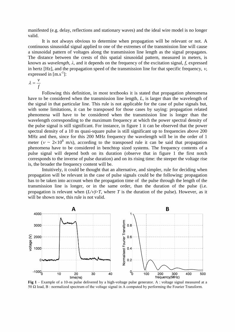
the pulse signal is still significant. For instance, in figure 1 it can be observed that the power

spectral density of a 10 ns quasi-square pulse is still significant up to frequencies above 200

MHz and then, since for this 200 MHz frequency the wavelength will be in the order of 1

meter ( ~ 2108 m/s), according to the transposed rule it can be said that propagation

phenomena have to be considered in benchtop sized systems. The frequency contents of a

pulse signal will depend both on its duration (observe that in figure 1 the first notch

corresponds to the inverse of pulse duration) and on its rising time: the steeper the voltage rise

is, the broader the frequency content will be.

Intuitively, it could be thought that an alternative, and simpler, rule for deciding when

propagation will be relevant in the case of pulse signals could be the following: propagation

has to be taken into account when the propagation time of the pulse through the length of the

transmission line is longer, or in the same order, than the duration of the pulse (i.e.

propagation is relevant when (L/)>T, where T is the duration of the pulse). However, as it

will be shown now, this rule is not valid.

Fig 1 – Example of a 10-ns pulse delivered by a high-voltage pulse generator. A : voltage signal measured at a

50 Ω load, B : normalized spectrum of the voltage signal in A computed by performing the Fourier Transform.

As it has been mentioned, in conventional electroporation, propagation related

phenomena are generally neglected. This is not surprising when it is taken into consideration

that cables between the electrodes and the generator are shorter than one or two meters and

that propagation speeds are in the order of 2108 m.s

-1; it would take 10 ns for an electrical

signal to travel along two meters of cable, which is negligible compared to the total duration

of the pulse (i.e. (L/) << T).

Nevertheless, it must be noted that the impact of propagation related phenomena on

pulse signals with a duration larger than 1 μs can actually be noticed if careful observations

are performed. For instance, figure 2 shows the result of a simulation in which a 100 μs pulse

is delivered to a 10 resistance through a cable with a propagation delay of 7.5 ns

(equivalent to 1.5 meters). At first glance, it can be observed that the voltage signals at the

generator (Vin) and at the load (Vout) are apparently identical. However, if the attention is

focused on the pulse edges then it can be noticed that both signals are not strictly identical;

Vout appears to be delayed and "softened". This distortion is not only due to mere propagation

but also to a propagation related phenomena that is later described: signal reflections occur at

the connections between the three different elements of the system (generator, cable and

resistance).

Fig 2 – Simulated example of the influence of propagation related phenomena on the shape of a 100 μs pulse.

This is a SPICE simulation (LTspice IV by Linear Technology Corp.) in which the voltage at a 10 load (Vout)

was monitored when pulses (Vin) from a 0 output impedance generator were delivered through a transmission

line with propagation delay of 7.5 ns (equivalent to 1.5 m) and a characteristic impedance of 50 (these

concepts are later explained in section 1.2).

Therefore, propagation related phenomena actually do have an impact on the signals

typically used in conventional electroporation. However, this impact is only significant on the

pulse edges and, in terms of biological consequences, it has been demonstrated that the shape

of those edges is not relevant in conventional electroporation (Kotnik et al 2001a).

1.2 Behavior of a transmission line

1.2.1 Propagation phenomenon

This section presents a classical electrical model for transmission lines (e.g. a coaxial

cables) that reveals the propagation phenomenon.

For the whole length of the transmission line, the model consists of a succession of

small electric sub-circuits each of which has a infinitesimal length, dx, very small compared

to the wavelength. Because of their short length, in each sub-circuit it is possible to ignore the

propagation phenomenon and then simple circuit theory analysis can be applied. Each sub-

circuit (figure 3) is modeled by a series inductance (L = l.dx [H], l is the linear inductance

[H.m-1

]) and a parallel capacitance (C = c.dx [F], c is the linear capacitance [F.m-1

]). In

addition, more complete models include resistive elements (a series resistance with L and a

parallel conductance with C) which are responsible for an attenuation of propagated signals.

Nevertheless, signal attenuation, and hence those dissipative elements, are usually neglected if

the transmission line length does not exceed the wavelength by several orders of magnitude,

which is the case in nsPEF experimental setups.

Fig 3- A transmission line can be modeled as a succession of elementary sub-circuits in which the propagation

phenomenon can be neglected.

Then, despite the fact that each sub-circuit does not model the propagation

phenomenon, it is possible to demonstrate by means of differential equations that voltage

signals do propagate without distortion along the transmission line length (x) with an speed

equal to :

]m/s[1

lcv

The propagation speed is fixed by the linear capacitance and inductance of the

transmission line which are themselves imposed by the materials (especially the dielectric)

that compose the line and by the geometry of the transmission line. In the case of a coaxial

cable (presented on figure 4), approximate values for linear capacitance and inductance can be

evaluated by the following expressions:

1

2

101

2

1

0 H.m)(2

F.m

)(

2 r

rLogland

r

rLog

rc

Fig 4- Electrical characteristics of a common coaxial cable.

1.2.2 Characteristic impedance and reflections

It can be demonstrated that at any point of the transmission line, when the signal

propagates from the pulse generator to the biological load (+ direction), the voltage (V(x)+)

and current (I(x)+) are related according to:

c

lwith

x

xcc

ZZI

V

The impedance introduced here, Zc, is called the characteristic impedance of the

transmission line and is expressed in ohms. A standard value for radio-communications

coaxial cables is 50 Ω.

The sample that is exposed to nsPEFs is commonly placed at the end of the cable and,

from an electrical point of view, it can be modeled as a load with complex impedance Z

(figure 5). If this load matches the characteristic impedance of the cable, i.e. when Z=Zc, then

the voltages and the currents at the two sides of transmission line termination (i.e. at the load

and at the transmission line) are the same. In this case, all the energy that was propagating in

the line is absorbed by the termination load. On the contrary, if Z≠Zc, a reflection will occur

and a voltage wave will start to propagate in the opposite direction through the transmission

line (i.e. from the load towards the pulse generator). This reflected wave is produced by the

following mechanism: the Ohm's law is valid at both sides of the transmission line

termination (i.e at the load and within the transmission line), therefore, since the voltage at

both sides of the termination is also the same, when Z≠Zc then it is required that a current is

generated in the opposite direction in order to obey the Kirchhoff's current law. This current

in turn generates the voltage wave (V(x)-= Zc.I(x)-). Once the reflected wave reaches the

generator, another reflected wave (in the + direction) will be generated if the impedance of the

generator (i.e. its output impedance) does not match the characteristic impedance.

Fig 5 – Reflection on the termination of the transmission line. When the voltage and current signals propagating

in the positive x-direction (V(x)+ ; I(x)+) reach a mismatched load, they are partially reflected. The reflected

signals (V(x)- ; I(x)-) propagate in the opposite direction.

When reflections occur, part of the energy contained in the pulse is absorbed by the

load and part of it is reflected. The fraction of energy transmitted to the load can be evaluated.

Results of computation for a 50 Ω cable and a resistive termination Rload, are plotted on figure

6. As displayed, transmitted power is maximum for the impedance matching condition and it

rapidly decreases for lower or larger load resistance values.

Fig 6 – Fraction of the energy transmitted to the load in the case of a resistive termination and a 50 Ω cable.

It is important to mention that not only the amount of energy transmitted to the load

will be affected by reflection. Levels and shapes of voltage and current signals can be

dramatically different from the ones initially coming out of the generator. Indeed, the voltage

at the load and the current that runs through it are the sum of the initial signals and the

reflected ones:

)()()()()()( 000000 xVxVxVandxIxIxI

These relations are also true in the frequency domain:

)()()()()()( 000000 xxxandxxx VVVIII

The magnitudes and phases of the reflected signals can be expressed as functions of the initial

signals defining the complex reflection coefficients ΓV and ΓI.

V

cload

loadcI

cload

cloadV

x

xand

x

xΓ

ZZ

ZZ

I

IΓ

ZZ

ZZ

V

VΓ

)(

)(

)(

)(

0

0

0

0

Most striking examples of impedance mismatch are observable in extreme cases: a

perfect short-circuit and a perfect open circuit. These examples are illustrated in figure 7.

When the load is an open circuit, the voltage amplitude of the pulse at the load terminals is

twice the amplitude of the pulse that was travelling from the generator. On the other hand, if

the load is a short-circuit, the voltage amplitude at the load will be null.

Fig 7 – Illustration of reflection for two different loads. A pulse generator is connected to a load through a

transmission line (length L ; propagation speed ν). If the load is a short circuit (a), the pulse is totally reflected in

phase opposition and the resulting voltage on the load is null. If the load is an open circuit (b), the pulse is totally

reflected in phase and the resulting voltage is twice the generated one.

As a consequence, it appears that for a given pulse generator and cable, the applied signals,

and in particular the applied voltage, will be highly dependent on the impedance of the

exposure device which in turn will depend on the properties of the biological sample.

1.3 Impedance matching for exposure devices

One of the common ways of doing in-vitro experiments is to use commercial

electroporation cuvettes filled with cell suspensions (Garon et al. 2007, Kolb et al. 2006).

Typical dimensions for such cuvettes are: an electrode area S of 1 cm2 and an electrode

separation l of 1 mm (volume = 0.1 ml). With these dimensions, a cuvette filled with a

solution with a conductivity of σ = 1 S/m would have a resistance R ([Ω]) of approximately:

10.1

S

l

σR

If a 10 kV pulse was applied through a 50 Ω cable to such a cuvette, the resulting

voltage according to the reflection coefficients would be 3.3 kV. In order to minimize such

voltage drop, it is possible to adjust the conductivity of the solution or to modify the

geometrical characteristics of the cuvette so that the load impedance is better matched to the

characteristic impedance of the cable. Unfortunately, the experimental conditions narrow the

degrees of freedom for such kind of solutions. For instance, although it is possible to reduce

the conductivity of a cell suspension medium without altering its osmolarity by adding non-

ionic agents (e.g. sucrose), the biological consequences of an extreme depletion of

extracellular ions will add uncertainty to the interpretation of the observations.

Alternative solutions can be based on modifying the other elements of the system. For

instance, it is possible to interconnect multiple generators in order to change the total source

impedance or even to build an adapted generator (Hall et al. 2007). Another feasible solution

is to insert a matching impedance in parallel with the load in those cases in which the sample

has a high impedance. Some examples of this approach can be found for single cell exposure

(Pakhomov et al. 2007). In this configuration most electrical power will be transmitted to the

matching impedance and not directly to the biological sample.

In general, both, the resistive, R, and the reactive, X, components of the biological

sample impedance (Z = R + jX) will be significant at the frequencies of interest. Then, since

the characteristic impedance of most transmission lines is purely resistive (Zc= 50 + j0 )

some degree of pulse distortion will be almost unavoidable. In radio-communications it is

possible to match reactive impedances by inserting compensating circuits. However, such

compensating circuits are only useful for a single frequency or for a narrow bandwidth, which

is not the case in pulse transmission.

Finally, it must be mentioned that the electrical connection from the transmission line

to the sample will also contribute by itself to the global impedance of the load. Indeed, to

connect a cuvette to a coaxial cable for in vitro experiments, a cuvette holder is necessary.

Similarly, for performing in vivo experiments electrodes and connectors are necessary. These

connections will basically add parasitic capacitances and inductances to the sample. An

essential rule to limit parasitic effects is to make the connection as short as possible both to

avoid propagation phenomena and to minimize inductive and capacitive parasitic elements.

In conclusion, even if all the issues described above are carefully addressed when

implementing the experimental setup, distortion cannot be fully avoided. As a consequence,

nsPEFs delivery must be accompanied by monitoring of the signal waveforms.

2. Breakdown of dielectric materials

The so-called dielectric strength of an electrically insulating material indicates the

maximum electric field that the material can withstand without experiencing an abrupt failure

of its insulating properties, either reversible or irreversible. Such failure in isolation is known

as electrical breakdown and it has been observed to occur in dielectric solids, gases and

liquids. Dry air at atmospheric pressure has a dielectric strength of about 3 MV/m,

polytetrafluoroethylene (TeflonTM

) has a dielectric strength higher than 60 MV/m, for alumina

that value is about 13 MV/m, for polystyrene is about 20 MV/m and for fused silica it is

possible to measure dielectric strength values above 400 MV/m. Breakdown process typically

develops within a few nanoseconds (Beddow et al. 1966) and, for most materials, it is

believed that the main phenomenon responsible for it is the avalanche breakdown: if the

electric field is strong enough, free electrons in the dielectric material, either preexisting or

freed by the electric field, are accelerated by the electric field and liberate additional electrons

when colliding with the atoms of the material (i.e. ionization) so that the number of free

charged particles is thus increased rapidly in an avalanche-like fashion. In the context of the

present book, it is interesting to note that cell membrane electroporation is a case in which

avalanche breakdown does not seem to be involved in the insulation failure process (Crowley

1973).

Transmission lines consist of metallic conductors and dielectrics. It is obvious then

that the maximum voltage that a transmission line will be able to withstand will depend on the

geometrical features of the line (e.g. the separation distance between conductors) and the

dielectric strength of the dielectric material. A typical RG-58/U coaxial cable employed in

10BASE2 Ethernet computer networks and for radio-communications is specified to

withstand 1500 VDC between the inner conductor and the shield whereas a RG-194/U coaxial

cable, intended for pulse transmission, can withstand DC voltages above 30 kV. Such increase

in voltage tolerance comes with the drawback of a larger diameter (5 mm for the RG-58/U

against 50 mm for the RG-194/U) and an increase of mechanical stiffness.

The same kind of considerations have to be applied to the connectors between the

transmission lines and the exposure chamber or the pulse generator. Furthermore, an aspect

that must be carefully taken into account is that the dielectric strength of air is particularly low

(3 MV/m) and sparks (i.e. dielectric breakdown) may occur easily at open connectors or

between the electrodes of the exposure chamber. These sparks will probably not be

destructive but they will prevent proper application of the pulses to the sample. On the other

hand, it is convenient to mention that for solid dielectrics even a single breakdown event can

severely degrade permanently the insulating capabilities of the material.

3. Monitoring of an ultra short electric signal

3.1 Choice of suitable probes

As pointed above, it is advisable to capture and observe the signals that are actually

applied to the exposure chamber. Besides the voltage signal, it can also be convenient to

monitor the current that flows through the sample.

The first stage in the acquisition chain consists of the so-called probes. A high-voltage

probe scales down the voltage to levels tolerable by the next stage in the acquisition chain

(e.g. a 50 oscilloscope input typically tolerates voltage amplitudes of about 1V) whereas a

current probe transforms the current signal into a voltage signal. High-voltage probes are

usually based on resistive voltage dividers and high-current probes are generally based on the

Hall effect. The specific features of the nsPEFs (high voltage, high current and high

bandwidth) impose some serious design constraints for the probes and, as consequence, only

a handful of suppliers commercialize suitable probes. Probes useful for monitoring nsPEFs

signals are typically employed in applications that involve similar signal features (e.g. Ultra

Large Band Radar and plasma generation)

A fundamental limitation of high-voltage probes and current probes is their

bandwidth. Typically these probes behave as first-order low-pass filters and their cut-off

frequency will determine to a large extent the fidelity of the whole acquisition system. For

instance, the simulations depicted in figure 8 show the response to a 16 ns pulse (including 3

ns + 3 ns rise and fall times) when three voltage probes with different cut-off frequencies are

employed: 0.1 GHz, 1 GHz and 10 GHz. As it can be noticed, a voltage probe with a cut-off

frequency of 0.1 GHz (trace b) would not only dramatically distort the shape of the original

signal but it would also yield an underestimation of the pulse amplitude (70 V instead of 100

V).

Fig 8 – Time behavior of voltage probes with different cut-off frequencies. Responses (traces b,c and d) have

been obtained from SPICE simulations (MacSpice) under the assumption that probes behave as first-order low-

pass filters. The simulated original signal (trace a) has an amplitude of 100 V and a duration of 16 ns (including

3 ns + 3ns rise and fall times).

As an alternative to high-voltage probes it is possible to employ tap-offs, also known

as power dividers or splitters, inserted in the transmission line. These components are

particularly interesting as they allow a direct visualization of the reflections.

3.2 Monitoring devices

Once the high-voltage and current signals have been transformed into low-voltage

signals, it is required to capture them and to digitalize them before proceeding to the

subsequent monitoring stages (e.g. storage, parameterization and visualization). Different

solutions can be adopted in order to perform all the required steps but, in terms of

convenience, modern digital oscilloscopes probably outperform all other approaches. Digital

oscilloscopes integrate signal acquisition elements together with visualization elements (i.e.

display), data storage and parameterization mathematical tools (e.g. automatic quantification

of pulse amplitude and width).

The particular features of the nsPEFs signals impose at least two specific

characteristics of the monitoring system: 1) large acquisition bandwidth and 2) large memory.

Signal acquisition bandwidth is largely determined by the sampling rate of the analog

to digital converter (ADC) embedded within the acquisition system. The Nyquist-Shannon

theorem states that it is sufficient to sample at a rate twice higher than the bandwidth of the

input signal in order to be able to reconstruct accurately the original waveform. However,

oversampling, that is, digitalizing the signal at a higher frequency than twice the bandwidth of

the signal being sampled, is commonly performed in signal acquisition systems as it provides

some advantages in terms of noise cancellation and facilitates the design of the system. As a

matter of fact, digital oscilloscopes generally have sampling rates well above three times the

maximum input bandwidth.

A second important feature, especially in case of acquisition of long trains of pulses, is

the memory available for the storage of the acquired data. A single 10 ns pulse sampled at 50

GS/s will only require 500 points of memory. However, a single pause of 100 ms between

two pulses in a train of pulses (i.e. pulse repetition frequency of 10 Hz) will fill 5109 points

of memory which is well above the memory depth of current scopes. Fortunately, current

high-performance oscilloscopes include a memory segmentation function that allows to

record all the “interesting” points whereas the “dull” ones are disregarded: when a pulse is

detected (i.e. oscilloscope trigger), only a limited number of samples before and after the

trigger is recorded so that only the time segments corresponding to the pulses are recorded

sequentially in memory. Later on, all the useful information concerning the applied pulses

(e.g. amplitude, duration, rise and fall times) can be assessed.

4. Side effects of the application of pulsed electric fields Administration of pulsed electric fields to biological samples can be accompanied by

phenomena not related to the direct effects of the electric fields on biological structures and

their constituents. These phenomena, which could be labeled as interfering phenomena, must

be taken into account and, if possible, avoided in order to simplify the interpretation of the

experimental results. Phenomena such as cell electrodeformation (due to Maxwell stress) or

ionization of macromolecules should not be included within this category as they are in fact a

direct consequence of the pulses on the constituents of the biological sample.

Here we briefly introduce and discuss two groups of interfering phenomena caused by

application of high field pulses: 1) thermal effects and 2) electrochemical effects. Our

description of both families of phenomena is focused on nsPEFs but most of what is said here

can be applied also to pulses employed in conventional electroporation.

4.1 Thermal effects

Electrical power is dissipated as heat at any conductor. This phenomenon is known as

Joule heating but it is also referred to as ohmic heating or resistive heating because of its

relationship with Ohm's law (V=IR):

GVR

VRIIVPdissipated

22

2

where Pdissipated is the total amount of heat power generated in the whole conductor (expressed

in watts, [W]), V is the applied voltage (volts, [V]), I is the current that flows through the

conductor (amperes, [A]), R is the resistance of the conductor (ohms, [Ω]) and G is the

conductance of the conductor (inverse of the resistance, expressed in siemens, [S]).

The above equation is intended for two-terminal components (e.g. a piece of wire). For

infinitesimal volumes the Ohm's law can be expressed as:

J

Eρ

where ρ is the resistivity of the material (ohmsmeter,[Ω.m]), |E| is the local magnitude of the

electric field ([V/m]) and |J| is the magnitude of the current density ([A/m2]). And now it is

possible to write down an expression for the dissipated power due to Joule heating in an

unitary volume (pdissipated, expressed in W/m3):

2

2

EE

JE σρ

pdissipated

where σ is the conductivity of the material (inverse of ρ, [S/m]).

If it is assumed that no heat exchange occurs within the conductive material and

between the material and its environment (i.e. the worst case scenario if sample heating is

undesirable), then the increase in temperature at each sample point (ΔT) can be easily

calculated as:

dc

tσ

dc

UΔT heat

2E

where t is the time ([s]), Uheat is the applied thermal energy (= power time, expressed in

joules, [J]=[W.s]), c is the specific heat capacity of the material (joules/(gramskelvin),

[J/(g.K)]) and d is the mass density of the material ([g/m3]).

If a single 10 ns pulse of 1 MV/m (10 kV/cm) is applied to a cell suspension in a

highly conductive medium (σ=1.5 S/m), the maximum temperature increase that can be

expected is only 0.0036 K (cwater = 4.184 J/(g.K), dwater = 0.997×106 g/m

3), which is negligible

under biological experimental conditions. On the other hand, if longer or larger pulses are

considered then the temperature jumps can start to be significant. For instance, a single pulse

of 5 MV/m and 50 ns would produce a temperature rise of about 0.45 degrees which is

probably still too low to cause observable biological effects; particularly taking into account

that such temperature increase will only last for a few seconds or fractions of a second in

actual setups in which heat dissipates. However, it must be noticed that pulses are commonly

applied at repetition frequencies of 1 Hz or higher and, in these cases, temperature can build

up if heat does not dissipate rapidly enough. In such cases it is highly advisable to perform

thermal measurements (e.g. by means of fiber optic thermal sensors or infrared cameras,

which are both fast and free of pulse interference) or to perform numerical thermal modeling

of the system (Davalos et al. 2005).

The maximum tolerable temperature increase will depend on the experimental

conditions and on the objectives of each biological study. As stated by Diller et al. (Diller et

al. 1999), damage to biological structures resulting from elevated temperatures is very

sensitive to the value of the highest temperature that is reached and less so to the time of

exposure, but, of course, both factors are important. Nevertheless, although some models have

been implemented to describe such double dependency (Diller et al. 1999), and have been

applied for electroporation (Maor et al. 2008), until now most studies in conventional

electroporation and in the nsPEF field only consider a maximum value for the temperature

increase as the criterion for tolerability. In particular, researchers in the nsPEF field consider

that temperature rises of about some tenths of kelvin (Schoenbach et al. 2001, Vernier et al.

2004) or of a few kelvins (Deng et al. 2003, Nuccitelli et al. 2006) are perfectly tolerable in

their studies.

It must be noted that Joule heating depends on the square of the electric field

magnitude. This fact implies that field distribution heterogeneities will have a significant

impact on heating. For instance, high electric fields around the electrodes due to the edge

effect may cause local thermal burns after nsPEFs administration in the same way that has

been observed in conventional tissue electroporation (Edd et al. 2006). Moreover, Vernier et

al. hypothesized that field distribution heterogeneities at cell or sub-cellular level could cause

thermal differences at microscopic level, but those were not noticed in their study (Vernier et

al. 2004).

Temperature plays an important role in ionic conductance: viscosity of the solvent

decreases as temperature rises, increasing ion mobility and, consequently, increasing electrical

conductivity. Although such dependence is not very significant (for most aqueous ionic

solutions the temperature dependence of conductivity is about + 2 %/K) this phenomenon can

in turn have a slight effect on the temperature: as temperature increases due to Joule heating,

conductivity increases and therefore Joule heating further increases which accelerates

temperature climb.

Finally, we want to point out another temperature-related phenomenon that may have

some biological significance: water thermal expansion. When liquid water is heated, its

volume increases and, if such volume increase is confined or cannot disperse sufficiently

rapidly, as it happens in the case of short thermal bursts, then pressure increases according to

the equation:

ΔTΔP

where ΔP is the resulting pressure increase, is the thermal expansion coefficient of water

(207 10-6

K-1

), is the compressibility coefficient of water (4.6 10-4

Pa-1

) and ΔT is the

applied temperature increase. This sudden increase in pressure may have some effect by itself

at the location where it is created but it can also affect distant locations as it causes a

shockwave that propagates. In fact, this phenomenon has been proposed as a mechanism to

generate shockwaves for lithotripsy treatments as an alternative to underwater sparks (US

patent 6,383,152 B1). Nevertheless, it does not seem very plausible that this phenomenon

could have significant biological consequences. A sudden increase in temperature of 0.5

degrees would imply an increase in pressure of about 225 kPa (2.2 atm). This figure may

seem important but in fact is almost negligible taking into account that lithotripsy

shockwaves have pressures of about 100 atm and are only effective on hard materials (e.g.

kidney stones) and not on soft tissues.

4.2 Electrochemical effects

When DC currents are forced to flow through the interface between an electronic

conductor (e.g. a metal) and an ionic conductor (e.g. biological media), oxidation and

reduction chemical reactions (“redox” reactions) occur which involve the molecules of the

metal (electrode) and those of the ionic media (electrolyte) in a process called electrolysis.

Some of the resulting chemical species liberated into the media can interfere with the

biological processes up to the point of compromising cell viability. As a matter of fact, at

present, electrochemical reactions are intentionally caused with low level currents applied

through metallic needles for the ablation of solid tumors in a procedure called electrochemical

treatment (EChT) (Nilsson et al. 2000).

In comparison to Joule heating, electrochemical effects are fundamentally

accumulative: the chemical species created by electrolysis will accumulate pulse after pulse;

although some molecules will finally escape as gas or will recombine with molecules in the

media to form neutral species.

The main reactions that are believed to occur in biological samples when inert

electrodes (e.g. platinum) are employed are (Nilsson et al. 2000, Saulis et al. 2005):

1) 2H2O + 2e- H2 (gas) + 2OH

- at the cathode.

2) 2H2O O2 (gas) + 4H++4e

- at the anode.

3) 2Cl- Cl2 (gas) + 2e

- also at the anode.

Furthermore, if instead of inert electrodes, electrochemically soluble electrodes (e.g. copper,

aluminum or stainless steel) are employed, then other oxidation reactions that release metallic

ions can also occur at the anode (Kotnik et al. 2001b), such as (Saulis et al. 2005):

4) 2Al 2Al+3

+ 6e-

The biological significance of each one of the above reactions and their resulting species is

still a matter of debate. Nevertheless, it is believed that H+ production at the anode (i.e. pH

decrease) is particularly important in EChT (Nilson et al. 2000) whereas release of Al+ ions

has been found to alter Ca2+

homeostasis in cell cultures (Loomis-Husselbee et al. 1991).

Faraday's laws of electrolysis indicate that the amount of substance (M), measured in

moles (i.e. number of molecules), produced by the above electrochemical reactions will be

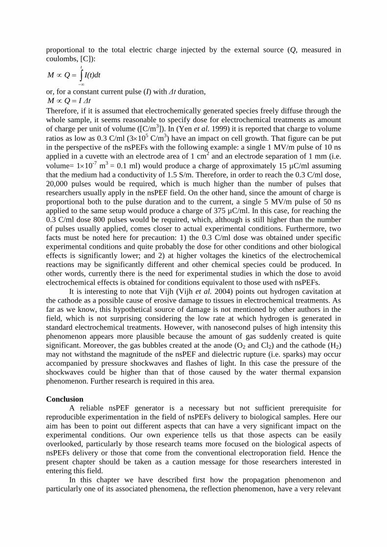
proportional to the total electric charge injected by the external source (Q, measured in

coulombs, [C]):

t

I(t)dtQM

or, for a constant current pulse (I) with Δt duration,

ΔtIQM

Therefore, if it is assumed that electrochemically generated species freely diffuse through the

whole sample, it seems reasonable to specify dose for electrochemical treatments as amount

of charge per unit of volume ([C/m3]). In (Yen et al. 1999) it is reported that charge to volume

ratios as low as 0.3 C/ml (3105 C/m

3) have an impact on cell growth. That figure can be put

in the perspective of the nsPEFs with the following example: a single 1 MV/m pulse of 10 ns

applied in a cuvette with an electrode area of 1 cm2 and an electrode separation of 1 mm (i.e.

volume= 110-7

m3

= 0.1 ml) would produce a charge of approximately 15 µC/ml assuming

that the medium had a conductivity of 1.5 S/m. Therefore, in order to reach the 0.3 C/ml dose,

20,000 pulses would be required, which is much higher than the number of pulses that

researchers usually apply in the nsPEF field. On the other hand, since the amount of charge is

proportional both to the pulse duration and to the current, a single 5 MV/m pulse of 50 ns

applied to the same setup would produce a charge of 375 µC/ml. In this case, for reaching the

0.3 C/ml dose 800 pulses would be required, which, although is still higher than the number

of pulses usually applied, comes closer to actual experimental conditions. Furthermore, two

facts must be noted here for precaution: 1) the 0.3 C/ml dose was obtained under specific

experimental conditions and quite probably the dose for other conditions and other biological

effects is significantly lower; and 2) at higher voltages the kinetics of the electrochemical

reactions may be significantly different and other chemical species could be produced. In

other words, currently there is the need for experimental studies in which the dose to avoid

electrochemical effects is obtained for conditions equivalent to those used with nsPEFs.

It is interesting to note that Vijh (Vijh et al. 2004) points out hydrogen cavitation at

the cathode as a possible cause of erosive damage to tissues in electrochemical treatments. As

far as we know, this hypothetical source of damage is not mentioned by other authors in the

field, which is not surprising considering the low rate at which hydrogen is generated in

standard electrochemical treatments. However, with nanosecond pulses of high intensity this

phenomenon appears more plausible because the amount of gas suddenly created is quite

significant. Moreover, the gas bubbles created at the anode (O2 and Cl2) and the cathode (H2)

may not withstand the magnitude of the nsPEF and dielectric rupture (i.e. sparks) may occur

accompanied by pressure shockwaves and flashes of light. In this case the pressure of the

shockwaves could be higher than that of those caused by the water thermal expansion

phenomenon. Further research is required in this area.

Conclusion

A reliable nsPEF generator is a necessary but not sufficient prerequisite for

reproducible experimentation in the field of nsPEFs delivery to biological samples. Here our

aim has been to point out different aspects that can have a very significant impact on the

experimental conditions. Our own experience tells us that those aspects can be easily

overlooked, particularly by those research teams more focused on the biological aspects of

nsPEFs delivery or those that come from the conventional electroporation field. Hence the

present chapter should be taken as a caution message for those researchers interested in

entering this field.

In this chapter we have described first how the propagation phenomenon and

particularly one of its associated phenomena, the reflection phenomenon, have a very relevant

impact on the pulse field that is actually applied to the sample. Then we have explained that,

up to a point, it is possible to control those reflections by matching the impedance of the

exposure cell. Nevertheless, due to the uncertainties of this impedance matching process, we

consider that voltage and current monitoring systems are highly advisable and we have given

some indications about the use of these systems and their limitations. Furthermore, since high-

voltage is a fundamental attribute of nsPEF signals, we have provided some details on the

electrical breakdown phenomenon.

Finally, we have discussed two groups of side effects of the application of nsPEFs:

electrochemical and thermal effects. Actually, both families of phenomena are also present in

the case of conventional electroporation. The extremely short duration of the nsPEFs does not

necessarily avoid the problems related to the electrochemical formation of chemical species at

the electrode-sample interface. Temperature rise because of the Joule effect will be

particularly significant if the nsPEF application comprises a train of pulses at a high repetition

frequency.

NsPEF can be an extraordinary tool for intracellular electromanipulation. The use of

nsPEFs may raise many hopes in terms of improvement of our knowledge in cell biology and

cell functioning, as well as in terms of development of new biotechnological and biomedical

applications. The future will confirm these hopes or prove them wrong. In any case, only

well-controlled experimental conditions will result in robust and reproducible biological

effects and in their translation into interesting applications.

Acknowledgements

The work of the authors is supported by grants of the CNRS, Institut Gustave-Roussy,

Univerité Paris-Sud, EU 6th

FP (CLINIGENE - FP6, LSH-2004-018933), INCA (Institut

National of Cancer, France - contract number 07/3D1616/Doc-54-3/NG-NC),

DGA/D4S/MRIS (contract number 06 34 017) and French National Agency (ANR) through

Nanoscience and Nanotechnology Program (Nanopulsebiochip n° ANR-08-NANO-024-01)

References

Beddow, AJ. Brignell, JE. 1966. Nanosecond breakdown time lags in a dielectric liquid.

Electronics Letters 2: 142-143.

Crowley, J.M. 1973. Electrical breakdown of bimolecular lipid membranes as an

electromechanical instability, Biophys. J.,13: 711-724.

Davalos, R.V. Mir, L.M. Rubinsky, B. 2005. Tissue ablation with irreversible electroporation.

Annals of Biomedical Engineering 33: 223-231.

Deng, J. Schoenbach, KH. Buescher, ES. Hair, PS. Fox, PM. Beebe, SJ. 2003. The effects of

intense submicrosecond electrical pulses on cells. Biophys. J. 84: 2709-2714.

Diller, K.R. Pearce, J.A. 1999. Issues in modeling thermal alterations in tissues. Annals of the

New York Academy of Sciences 888: 153-164.

Edd, J.F. Horowitz, L. Davalos, R.V. Mir, L.M. Rubinsky, B. 2006. In vivo results of a new

focal tissue ablation technique: irreversible electroporation. IEEE Trans. Bio-Med. Eng. 53:

1409-1415.

Garon, EB. Saweer, D. Vernier, PT. et al. 2007. In vitro and in vivo evaluation and a case

report of intense nanosecond pulsed electric field as a local therapy for human malignancies.

Int. J. Cancer 121: 675-682.

Hall, E.H. Schoenbach, K.H. Beebe, S.J. 2007. Nanosecond pulsed electric fields have

differential effects on cells in the S-Phase. DNA and Cell Bio. 26: 160-171.

Kolb, JF. Kono, S. Schoenbach, KH. 2006. Nanosecond pulsed electric field generators for

the study of subcellular effects. Bioelectromagnetics 27: 172-187.

Kotnik, T. Mir, L.M. Fisar, K. Puc, M. Miklavcic, D. 2001a. Cell membrane

electropermeabilization by symmetrical bipolar rectangular pulses. Part I. Increased efficiency

of permeabilization. Bioelectrochemistry. 54: 83-90.

Kotnik, T. Miklavcic, D. Mir, L.M. 2001b. Cell membrane electropermeabilization by

symmetrical bipolar rectangular pulses. Part II. Reduced electrolytic contamination.

Bioelectrochemistry 54: 91-95.

Loomis-Husselbee, J.W. Cullen, P.J. Irvine, R.F. Dawson, A.P. 1991. Electroporation can

cause artefacts due to solubilization of cations from the electrode plates. Aluminum ions

enhance conversion of inositol 1,3,4,5-tetrakisphosphate into inositol 1,4,5-trisphosphate in

electroporated L1210 cells. Biochem. J. 277: 883-885.

Maor, E. Ivorra, A. Rubinsky, B. 2008. Intravascular irreversible electroporation: theoretical

and experimental feasibility study. Conference Proceedings: Annual International Conference

of the IEEE Engineering in Medicine and Biology Society. IEEE Engineering in Medicine and

Biology Society. Conference 2008: 2051-2054.

Nilsson, E. Von Euler, H. Berendson, J. et al. 2000. Electrochemical treatment of tumours.

Bioelectrochemistry 51: 1-11.

Nuccitelli, R. Pliquett, U. Chen, X. et al. 2006 Nanosecond pulsed electric fields cause

melanomas to self-destruct. Biochem. Biophys. Res. Comm. 343: 351-360.

Pakhomov, A.G. Kolb, J.F. White, J.A. Joshi, R.P. Xiao, S. Schoenbach, K.H. 2007. Long-

lasting plasma membrane permeabilization in mammalian cells by nanosecond pulsed electric

field (nsPEF). Bioelectromagnetics 28:655-663.

Saulis, G. Lape, R. Praneviciūte, R. Mickevicius, D. 2005. Changes of the solution pH due to

exposure by high-voltage electric pulses. Bioelectrochemistry 67: 101-108.

Schoenbach, K.H. Beebe, S.J. Buescher, E.S. 2001. Intracellular effect of ultrashort electrical

pulses,” Bioelectromag. 22: 440-448.

Sun, Y. Vernier, PT. Bebrend, M. Marcu, L. Gundersen, MA. 2005. Electrode microchamber

for noninvasive perturbation of mammalian cells with nanosecond pulsed electric fields. IEEE

Trans. Nanobioscience. 4: 277-283.

Vernier, P.T. Sun, Y. Marcu, L. Craft, C.M. Gundersen, M.A. 2004. Nanoelectropulse-

induced phosphatidylserine translocation. Biophys. J. 86: 4040-4048.

Vijh, A.K. 2004. Electrochemical treatment (ECT) of cancerous tumours: necrosis involving

hydrogen cavitation, chlorine bleaching, pH changes, electroosmosis. Int. J. Hydrogen

Energy. 29: 663-665.

Yen, Y. Li, J.R. Zhou, B.S. Rojas, F. Yu, J. Chou, C.K. 1999. Electrochemical treatment of

human KB cells in vitro. Bioelectromagnetics 20: 34-41.