Na, J., Mahyuddin, M. N., Herrmann, G., Ren, X., & Barber, P. (2015).Robust adaptive finite-time parameter estimation and control for roboticsystems. International Journal of Robust and Nonlinear Control, 25(16),3045-3071. 10.1002/rnc.3247

Peer reviewed version

Link to published version (if available):10.1002/rnc.3247

Link to publication record in Explore Bristol ResearchPDF-document

University of Bristol - Explore Bristol ResearchGeneral rights

This document is made available in accordance with publisher policies. Please cite only the publishedversion using the reference above. Full terms of use are available:http://www.bristol.ac.uk/pure/about/ebr-terms.html

Take down policy

Explore Bristol Research is a digital archive and the intention is that deposited content should not beremoved. However, if you believe that this version of the work breaches copyright law please contactopen-access@bristol.ac.uk and include the following information in your message:

• Your contact details• Bibliographic details for the item, including a URL• An outline of the nature of the complaint

On receipt of your message the Open Access Team will immediately investigate your claim, make aninitial judgement of the validity of the claim and, where appropriate, withdraw the item in questionfrom public view.

1

INTERNATIONAL JOURNAL OF ROBUST AND NONLINEAR CONTROL Int. J. Robust Nonlinear Control 2014; 00:1-28 Published online XX XXX 2014 in Wiley Online Library (wileyonlinelibrary.com). DOI: XXXXXXX

Robust adaptive finite-time parameter estimation and control for robotic systems

Jing Na1 ∗, Muhammad Nasiruddin Mahyuddin2*, Guido Herrmann2*, Xuemei Ren3 and Phil Barber4

1 Faculty of Mechanical & Electrical Engineering, Kunming University of Science & Technology, Kunming 650500,China 2 Department of Mechanical Engineering, University of Bristol, Bristol, BS8 1TR, UK

3 School of Automation, Beijing Institute of Technology, Beijing 100081, China 4 Jaguar & Land Rover Cars Limited, Abbey Road,Whitley, Coventry, CV3 4LF, UK

SUMMARY

This paper studies adaptive parameter estimation and control for nonlinear robotic systems based on parameter

estimation errors. A framework to obtain an expression of the parameter estimation error is proposed first by

introducing a set of auxiliary filtered variables. Then three novel adaptive laws driven by the estimation error are

presented, where exponential error convergence is proved under the conventional persistent excitation (PE) condition;

the direct measurement of the time derivatives of the system states are avoided. The adaptive laws are modified via a

sliding mode technique to achieve finite-time (FT) convergence, and an online verification of the alternative PE

condition is introduced. Leakage terms, functions of the estimation error, are incorporated into the adaptation laws to

avoid windup of the adaptation algorithms. The adaptive algorithm applied to robotic systems permits that tracking

control and exact parameter estimation are achieved simultaneously in finite time using a terminal sliding mode (TSM)

control law. In this case, the PE condition can be replaced with a sufficient richness (SR) requirement of the command

signals, and thus is verifiable a priori. The potential singularity problem encountered in TSM controls is remedied by

introducing a two-phase control procedure. The robustness of the proposed methods against disturbances is

investigated. Simulations based on the ‘Bristol-Elumotion-Robotic-Torso II’ (BERT II) are provided to validate the

efficacy of the introduced methods.

Received 21 April 2014; Revised 21 August 2014; Accepted XXX.

KEY WORDS: adaptive control; parameter estimation, robotic systems; terminal sliding mode control; finite time convergence

1. INTRODUCTION Adaptive control [1, 2] for control systems with unknown (or immeasurable) parameters and dynamics has been widely

studied to achieve output tracking, where the unknown system parameters are online updated/estimated by using

control errors. With this framework, asymptotic tracking error convergence and the boundedness of the parameter

estimation can be proved. However, it may be questionable to claim that the parameter estimates converge to their true

∗ E-mail: najing25@ 163.com (Jing Na), nasiruddin@usm.my (Muhammad Nasiruddin Mahyuddin), g.herrmann@bris.ac.uk (Guido Herrmann)

2

values due to the lack of an online verification of the persistent excitation (PE) condition [1]. To further improve the

control performance as well as the parameter estimation, a composite adaptive law has been proposed in [3, 4], where

the parameter adaptation is driven by both the tracking error and the prediction error, i.e. an extra predictor has to be

designed. In [5], a new composite adaptive control was studied based on the robust integral-of-the sign-of-the-error

(RISE) technique for Euler-Lagrange systems with additive uncertainties, where semi-global asymptotic stability is

proved. Apart from the aforementioned results that incorporate the parameter estimation into the controller synthesis

[1, 3, 6], there are also other methods that take the parameter estimation as a part of an observer design. In [7], the

estimation of time-varying parameters was studied via a neural network observer. An adaptive observer was provided

in [8] to guarantee arbitrarily fast exponential convergence of both the estimated parameter and states to their actual

values. In [9], an identification approach based on variable structure systems (VSS) was developed for multi-input

multi-output nonlinear systems. However, the observer design may impose some specific assumptions, e.g. matching

condition [8], and it is not always easy to characterize the convergence rate, e.g. finite-time convergence.

It has been well-recognized that adaptive laws should preferably include some information on the parameter

estimation error to improve the estimation error convergence [5]. However, this is not a trivial issue since the parameter

estimation error is generally immeasurable or unknown. Recently, the desire to include parameter error information

into adaptive control designs has resulted in several developments. In [10], a novel parameter estimation scheme was

proposed that allows for exact reconstruction of unknown parameters in finite-time (FT). The salient feature of this

method lies in that the true parameter can be recovered at any time instant as long as the PE condition is satisfied. In the

subsequent work [11], the idea was incorporated into the control design, where the adaptation is driven by combining

the tracking error with the parameter error to achieve exponential convergence. It was noted that the algorithm

proposed in [10] needs to test online the invertibility of a regressor matrix and to compute the matrix inverse when it is

appropriate. Moreover, the introduced auxiliary matrix and vector in [10, 11] have an unstable integrator and thus may

increase (even to infinite values), which will result in instability phenomena in the adaptive system. Our recent work

[12, 13] proposed novel filter operations to remedy the aforementioned issues (e.g. infinite growth) and developed

several adaptive parameter estimation schemes, for which exponential and/or finite-time error convergence are proved

without using the derivative of the system states. In particular, the developed adaptations were incorporated into the

model reference adaptive control (MRAC) in [12] for a class of nonlinear systems, such that finite-time convergence of

both the tracking and parameter estimation can be achieved rather than exponential convergence as in [11].

As a specific kind of nonlinear multi-input-multi-output (MIMO) systems, robotic manipulators [14, 15] have been

widely used. Since the 1980s when a linear parameterization of nonlinear robot dynamics was introduced [3], adaptive

control of robotic systems has been of long interest, e.g. [3, 14, 16]. Computed-torque based adaptive control [3, 14]

has been widely adopted, where global error convergence can be guaranteed. For those robotic systems with unknown

nonlinearities or actuator dynamics, function approximators (e.g. neural networks [17-19] or fuzzy systems[20]) have

also been utilized. However, what limits the practical applicability of such adaptive controllers is that only ultimate

boundedness of the parameter estimation error can be proved. Moreover, some of these control algorithms use the robot

joint acceleration measurements (that are susceptible to noises) [21]. To achieve FT error convergence, the principle of

terminal sliding mode (TSM) control [22] was extended to robotic systems [23, 24], where the nominal robotic model

3

needs to be known and the inversion of the inertia matrix needs be to be online calculated. To relax the requirement of

system model knowledge, neural networks were incorporated into the TSM control design in [25, 26]; however, a

potential singularity problem may be encountered in the reaching phase. To avoid the singularity problem in TSM

control, a modified TSM manifold was adopted [25, 26], and a two-phase control scheme was introduced in [27] for

nth-order SISO systems. However, it is noted that the (finite-time) parameter estimation was not addressed in the

aforementioned TSM schemes.

To address these motivating questions, we revisit the adaptive parameter estimation and control design for a class of

nonlinear robotic systems with unknown parameters. The parameter estimation is first studied by extending our recent

work [12] for a class of general nonlinear systems, and three novel adaptive laws will be presented, which are solely

driven by the parameter estimation errors and thus independent of any predictor or observer design. For this purpose, a

set of auxiliary system variables are obtained by introducing stable filter operations on the system states, the regressor

vector and the input. The parameter error information is thus obtained explicitly and used for the parameter estimation

in constructing an adaptive law, where exponential error convergence is guaranteed, provided a filtered (integrated)

regressor matrix is positive definite (This can be fulfilled under the conventional PE condition). Furthermore, by

applying the sliding mode technique [28] for the adaptation, two improved adaptive laws are proposed with attractive

finite-time convergence properties. Another advantage is that the developed estimation approaches avoid the online

test for the invertibility of the regressor matrix and the direct computation of a matrix inverse in comparison to [10]. In

particular, the infinite growth and possible instability of the filtered integral regressor matrix are successfully avoided,

which are not necessarily prevented in [10, 11]. Moreover, we can prove that the parameter error converges to zero in

finite time. A simplified online verification of a convergence condition is also suggested, which is a relaxed alternative

for the usual PE-condition. These parameter estimation schemes are then applied to nonlinear robotic systems, where

the torque filtering method proposed in [14, 16] is further improved so that the robot joint acceleration are not required.

The proposed parameter estimation methods for the adaptive control of nonlinear robotic systems can achieve

finite-time tracking and parameter estimation simultaneously. In this case, the required PE condition can be

transformed into an a priori verifiable sufficient richness (SR) requirement on the control reference signals [29], i.e. the

rows of the regressor vector are linearly independent along a desired trajectory. In particular, a two-phase control

procedure is investigated to avoid the potential singularity problem in the adaptive TSM control design: the first phase

is to force the system states to enter a prescribed region in which the singularity does not occur by using a sliding mode

control with linear sliding plane and exponential error convergence; the second phase is to switch to a TSM control that

realizes finite-time error convergence. Consequently, finite-time convergence of the tracking error and the estimation

error can be guaranteed simultaneously. Finally, the robustness of the parameter estimation and the control designs

against external disturbances is studied. Simulations based on a humanoid Bristol-Elumotion-Robotic-Torso II (BERT

II) arm [16] are conducted to validate the efficacy of the proposed methods. It is shown that the parameter error based

adaptation can improve the performance upon the existing adaptive methods, and the proposed control can avoid the

singularity problem.

The main contribution of this paper can be summarized as:

1) A general continuous-time framework for parameter estimation is proposed to obtain the explicit parameter error

4

information by using the available system dynamics and the estimated parameters. This can be achieved by introducing

stable filter operations on the states, the regressor vector and the input signals.

2) Novel parameter error based adaptive parameter estimation algorithms are investigated for robotic systems;

knowledge of the robot joint acceleration is avoided and finite-time convergence can be proved. Moreover, the online

test of the invertibility of a regressor matrix and the computation of the matrix inverse are not required. A simple online

verification of a convergence condition, a relaxed alternative to the usual PE-condition, is provided.

3) A two-phase TSM control is developed to avoid the potential singularity problem in TSM control of robotic systems;

finite-time parameter estimation and tracking control are achieved. In this case, the required PE condition can be

represented as an a priori verifiable SR requirement on the control command signals. The robustness of the proposed

methods with disturbances is investigated.

The paper is organized as follows: three adaptive parameter estimation algorithms based on the parameter

estimation error are discussed in Section 2. Section 3 is devoted to study the parameter estimation of nonlinear robotic

systems; Section 4 proposes a singularity free adaptive TSM control for robotic systems with guaranteed parameter

estimation. Simulation results are provided in Section 5 and conclusions are outlined in Section 6.

2. ADAPTIVE PARAMETER ESTIMATION

We first study the parameter estimation for the following nonlinear system ( , ) ( , )x x u x uϕ θ= +Φ (1)

where nx∈ is the system state, mu∈ is the control input, Nθ ∈ is the unknown parameter vector to be estimated. ( , ) nx uϕ ∈ is a known function vector and ( , ) n Nx u ×Φ ∈ is the known regressor matrix. The functions

( , )x uϕ and ( , )x uΦ are bounded for bounded x and u .

To facilitate the parameter estimation, the following assumption is provided:

Assumption 2.1 The system state x and the control input u of system (1) are bounded and accessible for measurement.

Assumption 2.1 has been widely used in the estimation literature [8, 10]. This can be achieved via a control law ( )u v= for (1). Moreover, the state x and input u are required, but the derivative x is not used in our estimation

schemes. Essential to this paper are the concepts of persistent excitation in combination with finite time convergence. Both concepts are here introduced separately:

Definition 2.1 [2] A vector or matrix function φ is persistently excited (PE) if there exist 0, 0T ε> > such that

( ) ( ) , 0t T T

tr r dr I tφ φ ε

+≥ ∀ ≥∫ . ◊

Lemma 2.1[30] For a continuous system ( , ), (0, ) 0, nx x t t xφ φ= = ∈

, there is a continuously differentiable positive-definite function ( , )V x t and real numbers 1 20,0 1c c> < < such that 2

1( , ) ( , )cV x t c V x t≤ − holds, then ( , )V x t converges to zero in

finite time with the settling time 210 0

1 2

1 ( ( ), )(1 )

cT V x t tc c

−≤−

for any given initial condition 0( )x t . ◊

Unlike available results, e.g. [7, 8, 10], which are dedicated to estimate unknown parameters θ of (1) by means of observers or predictors, the parameter estimation methods to be presented are independent of any observer and

5

predictor design. In order to derive the parameter estimation, we define the filtered variables fx , fΦ , fϕ of ,x ( )xϕ

and ( , )x uΦ as

, (0) 0

, (0) 0, (0) 0

f f f

f f f

f f f

kx x x x

kkϕ ϕ ϕ ϕ

+ = =Φ +Φ = Φ Φ =

+ = =

(2)

where 0k > is a filter parameter. Then it can be obtained from (1) and (2) that f

f f f

x xx

kϕ θ

−= = +Φ (3)

Define an auxiliary filtered and ‘integrated’ regressor matrix P and vector Q as

, (0) 0

( ) / , (0) 0

Tf f

Tf f f

P P P

Q Q x x k Qϕ

= − +Φ Φ =

= − +Φ − − =

(4)

where 0> is another design parameter. Note that the authors [10] used a formulation similar to (4) but without the terms P and Q , which creates for P and Q unbounded integration operations. This is circumvented in this paper.

The solution of (4) is derived as ( )

0

( )

0

( ) ( ) ( )

( ) ( ) ( ( ) ( )) / ( )

t t r Tf f

t t r Tf f f

P t e r r dr

Q t e r x r x r k r drϕ

− −

− −

= Φ Φ = Φ − −

∫∫

(5)

We now define another auxiliary vector NW ∈ that can be calculated from P , Q as

ˆW P Qθ= − (6)

where θ is an estimation for the unknown parameter θ . Different adaptation laws for θ will be given in the following developments.

From (3) and (5), one can verify that Q Pθ= holds such that

ˆ ˆW P Q P P Pθ θ θ θ= − = − = − (7)

where ˆθ θ θ= − is the parameter estimation error. The positive definite property of matrix P (i.e. min ( ( )) 0P tλ σ> > )1 is important for parameter estimation. We will

prove that this condition can be fulfilled provided the original regressor vector ( , )x uΦ in (1) is PE.

Lemma 2.2 [12] The matrix P is positive definite satisfying min ( ( ))P tλ σ> for t T> and some 0σ > , 0T > , provided the regressor

matrix ( , )x uΦ is persistently excited. ◊

Proof It is shown that the transfer function 1/( 1)ks + in (2) is stable, minimum phase and strictly proper [2], then fΦ defined in (2) is PE once Φ defined in (1) is PE because fΦ is the filtered version of Φ . Moreover, based on

Definition 2.1, if fΦ is PE, there exist 0T > and 0ε > so that the inequality ( ) ( )t T T

f ftr r dr Iε

+Φ Φ >∫ holds for all

0t > . Since the inequality ( )

0( ) ( ) ( ) ( )

t tt r T T T Tf f f ft T

e r r dr e r r dr e Iε− − − −

−Φ Φ > Φ Φ >∫ ∫ holds for t T> , then

min ( ( )) 0P tλ σ> > holds with Teσ ε−= , i.e. P is positive definite. According to Lemma 2.2, the conventional PE condition of the regressor vector Φ is sufficient to guarantee that

1 Throughout this paper, max min( ), ( )λ λ⋅ ⋅ are defined as the maximum and minimum eigenvalues of the corresponding matrices.

6

P is positive definite. Thus, similar to other system identification and parameter estimation literature (e.g. [8, 10]), P can be retained positive definite by imposing a suitable control u and/or a dither PE signal on system (1). However, the direct online validation of the PE condition is difficult in particular for a nonlinear system. Thus, it will be shown that testing for the positive definiteness of P permits to numerically verify conditions of convergence of the adaptive algorithms suggested in this paper. This replaces tests for PE in the case of the suggested adaptation algorithms. Another alternative convergence condition will be provided in a later part of the paper.

From the fact Q Pθ= and the assumption that P is positive definite follows easily the following:

Corollary 2.1 Assume system (1) with P , Q in (5) satisfies min ( ( )) 0P tλ σ> > for all 0t > , then it follows 1P Qθ −= . ◊

Although Corollary 2.1 provides a possible parameter estimation, where the inverse matrix 1P− needs to be online calculated as in [10, 11], which may be difficult since it may lead to numerical problems. In the following development, we will present three online parameter estimation schemes based on the parameter error information W .

2.1 ADAPTIVE PARAMETER ESTIMATION We first propose an adaptive law to estimate θ with exponential error convergence. The adaptive estimation

algorithm for θ is provided by

ˆ Wθ = −Γ (8) with 0Γ > being a constant diagonal gain matrix. Then the following result holds:

Theorem 2.1 Consider system (1) with the parameter adaptive law (8), if the filtered regressor matrix P satisfies min ( ) 0Pλ σ> > ,

then the parameter error θ exponentially converges to zero with the convergence rate 11 max2 / ( )µ σ λ −= Γ . ◊

Proof

Consider the Lyapunov function as 11

12

TV θ θ−= Γ , the derivative 1V along (8) is obtained as

11 1 1

T T TV W P Vθ θ θ θ θ µ−= Γ = = − ≤ −

(9)

where 11 max2 / ( )µ σ λ −= Γ is positive for all 0t > . Based on Lyapunov’s Theorem [31] and (9), the error θ converges

exponentially to zero with the rate 1µ .

Remark 2.1 It is known that the inclusion of an appropriate parameter error in the parameter adaptations can improve the parameter

estimation performance [1]. In this paper, W derived in (7) contains the parameter error information Pθ , which is used explicitly in the parameter adaptation; no observer or predictor design is introduced in comparison to available results [3, 7, 8, 10]. Moreover, unlike [10, 11], the matrix P and vector Q are all bounded by introducing a forgetting

factor 0> .

2.2 FINITE-TIME PARAMETER ESTIMATION We further improve the adaptive law to achieve finite-time error convergence. The variables P , Q and W are

designed as in (4)~(6) , then the parameter θ is updated by

ˆTP WW

θ = −Γ (10)

where 0Γ > is a constant diagonal gain matrix. This leads to the following result:

7

Theorem 2.2

For system (1) with parameter adaptation (10) and min ( ) 0Pλ σ> > , the parameter estimation error θ converges to

zero in finite time at satisfying 1max(0) ( ) /at θ λ σ−≤ Γ . ◊

Proof

Consider the Lyapunov function as 12

12

TV θ θ−= Γ , then it can be verified using min ( ) 0Pλ σ> > and W Pθ= − that

the derivative of 2V can be derived as

12 2 2ˆ

T T TT T P W P PV P V

PP Qθ θθ θ θ θ µ

θθ−= Γ = − = − ≤ − ≤ −

−

(11)

where 12 max2 / ( )µ σ λ −= Γ is a positive constant. According to (11) and [28], finite-time convergence of the

parameter estimation error θ can be guaranteed, and the time to achieve 0θ = is estimated by 2 22 (0) /at V µ≤ .

Clearly, the convergence time at depends on the excitation level σ and the learning gain Γ , i.e. a higher excitation

level σ and larger learning gain Γ will lead to a smaller time at .

2.3 ONLINE LEARNING OF THE MATRIX INVERSE OF P

As shown above, a possible parameter estimation can be given by 1P Q θ− = , where the inverse matrix 1P− needs to

be calculated. In this subsection, we will propose an alternative adaptive law to learn the inverse of P online. Define an auxiliary matrix K as

Tf fK K K K= − Φ Φ

, 10(0) 0K K− = > (12)

where 0> is the positive constant used in (4), and fΦ is the filtered regressor given in (2). Consider the matrix

equality 1 1 1 0d dKK KK K Kdt dt

− − −= + = , we derive the solution of (12) as

( ) 1 10 00

( ) [ ( ) ( ) ] [ ( )]tt t r T t

f fK t e K e r r dr e K P t− − − − − −= + Φ Φ = +∫ (13)

where 10 0 (0) 0TK K K −= = > is the initial condition chosen as 0K Iη= with 0η > being a constant.

Furthermore, one can employ the singular value decomposition (SVD) for matrix P as ( )

0( ) ( )

t t r T Tf fP e r r dr USV− −= Φ Φ =∫ (14)

where 1( , , )nS diag s s= is a matrix with is being the singular values of matrix P , and U , V are unitary matrices. Then based on the fact that 0K Iη= is a diagonal matrix and (13), it follows

11 10[ ] ( ) ( )t t T t TK e K P U S e I V V S e I Uη η

−− − − − − = + = + = + (15)

Consequently, the matrix KP is derived as

1 1

1

( ) , ,t T Tnt t

n

ssKP V S e I SV Vdiag Vs e s e

ηη η

− −− −

= + = + +

(16)

Since lim 1itt

i

ss e η−→∞

=+

if min ( ) 0Pλ σ> > and , 0η > , and TVV I= , the matrix KP is represented as

( ) ( ) ( )K t P t I E t= − (17)

where1

( ) , ,t t

Tt t

n

e eE t Vdiag Vs e s e

η ηη η

− −

− −

= + +

converges to zero as t →∞ , i.e. lim ( ) 0t

E t→∞

= . Then we have

8

[ ]ˆ ˆKP Eθ θ θ θ θ= − = + − (18) An alternative parameter adaptive law can be given as

ˆˆˆ

KQKQ

θθθ−

= −Γ−

. (19)

Theorem 2.3

For system (1) with the adaptive parameter estimation θ given by (19) (based on Q in (4) and K in (12) for 1(0) 0K Iη− = > ) and min ( ) 0Pλ σ> > , then the estimation error θ converges to a residual set cθ ≤ in finite time,

where 0c > is a positive constant. ◊

Proof

Select a Lyapunov function as 13

12

TV θ θ−= Γ , then according to (19) and the definition of P and Q in (4), we can

calculate the derivative of 3V as

( )3 3 3 3

ˆˆˆ

T KQV KP E E E VKQ

θθ θ θ θ θ θ µ ρθ−

= − − − ≤ − − + ≤ − +−

(20)

where 13 max2 / ( )µ λ −= Γ is a positive constant, 3 2 Eρ θ= denotes the effects of the initial condition 0K . From

min ( ) 0Pλ σ> > and the discussion of equation (17), it follows lim ( ) 0t

E t→∞

= . Although the fact lim ( ) 0t

E t→∞

= and thus

3lim ( ) 0t

tρ→∞

= holds and θ is bounded, 3ρ is usually not zero in finite time since the initial condition cannot be set as

zero [4], i.e. 0η ≠ . Consequently, unlike Theorem 2.2, it cannot be claimed that θ converges to zero in finite time. However, 3ρ is bounded for all 0t ≥ since E and θ are bounded, i.e. there exists 0c > so that 3 cρ γ< holds with 0 1γ< < . Certainly, for sufficiently large time 0t > , the constant 0c > will be smaller. Define a compact set as

( ) 23 3: | ( ) /V cθ θ µΩ = ≤ , then for all ( )tθ ∉Ω , we have ( )

2 21max 3 3

1 ( ) ( ) /2

V cλ θ θ µ−Γ ≥ > and thus cθ > . In this

case, it follows ( )3 3 3 3 3 1 0V V c cµ ρ ρ γ≤ − + ≤ − + < − − < (21)

Consequently, the parameter error θ will ultimately enter the compact set Ω within finite time. The size of the compact set can be adjusted to be arbitrarily small by tuning c small, e.g. reduction of the initial condition η of the matrix 1(0)K − . The convergence rate can also be improved by increasing the learning matrix gain Γ .

A clearly simple approach for parameter estimation is given by the following Corollary:

Corollary 2.2 For system (1) with Q defined in (4) and K defined in (12), it follows lim

tKQ θ

→∞= if the regressor Φ is PE. ◊

The proof follows from the fact that 1P Q θ− = and KP I→ as t → +∞ . According to (17), it is shown that K converges to 1P− due to lim ( ) 0

tE t

→∞= . This is clearly different to the results

presented in [10], and thus the online check for the invertibility and the computation of the inverse of matrix P (when it is appropriate) can be avoided. However, the estimation error in this case only converges in finite time to a small bounded region around zero due to the initial condition 1(0) 0K Iη− = ≠ . In fact, with the help of the auxiliary matrix

K , a practical test for the convergence condition of the algorithm of (19) or of Corollary 2.2 is carried out by verifying KP I≈ , implying non-singularity of P . This can be conducted online as shown in Section 5 for a simulation example.

Remark 2.2 From equation (17), the condition of lim ( ) ( )

tK t P t I

→∞= and lim ( ) 0

tE t

→∞= are also satisfied if there are some constants

9

1 0σ > and 2 0σ > so that 2( )min 1( ) 0tP e σλ σ − −> > . In particular for 2 0σ> > , this permits an exponentially

decaying value of min ( )Pλ , implying also a different concept of excitation of ( , )x uΦ . All of the adaptation laws of (8), (10) and (19) hold an inherent forgetting mechanism, which avoids the windup of the adaptation mechanism [1]. This is achieved as W is an expression of the parameter error θ .

3. PARAMETER ESTIMATION OF ROBOTIC SYSTEM

In this section, we will apply the proposed adaptive parameter estimation algorithms for a class of robotic systems. For this purpose, appropriate filter operations will be introduced so that the measurements of the robot joint accelerations are avoided. We consider a n-degrees of freedom (DOF) nonlinear robotic manipulator modeled by

( ) ( , ) ( )M q q C q q q G q τ+ + = (22)

where , , nq q q∈ are the robot joint position, velocity and acceleration, respectively; nτ ∈ is the control

torque/force vector; ( ) n nM q ×∈ is the inertia matrix, ( , ) n nC q q ×∈ is the Coriolis/centripetal torque, viscous and nonlinear damping, and ( ) nG q ∈ represents the gravity torque. The following properties are given [3, 14] for robotic system (22):

Property 3.1 The matrix ( ) 2 ( , )M q C q q−

is skew-symmetric, such that

( ) 2 ( , ) 0, , ,T nx M q C q q x x q q − = ∀ ∈

(23)

Property 3.2 The left-hand dynamics of the robotic system (22) can be represented in a linearly parameterized form

( ) ( , ) ( ) ( , , )M q q C q q q G q q q qφ θ+ + = (24)

where Nθ ∈ is a constant parameter vector to be estimated, and ( , , ) n Nq q qφ ×∈ is the known regressor matrix.

Property 3.3 The matrix ( )M q is positive definite and satisfies ( ) MM q λ≤ for positive constant 0Mλ > .2

3.1 ADAPTIVE PARAMETER ESTIMATION

The regression matrix ( , , )q q qφ in (24) is a function of the robot joint acceleration measurement q , which is

sensitive to measurement noises. In this paper, as inspired by [14, 16], this regressor matrix will be reformulated, where auxiliary filtered variables are introduced to eradicate the need for the joint acceleration. Define alternative vectors as

( , ) ( )F q q M q q= and ( , ) ( ) ( , ) ( )H q q M q q C q q q G q= − + +

, then based on Property 3.2, one can derive

1

2

( , ) ( ) ( , )( , ) ( ) ( , ) ( ) ( , )

F q q M q q q qH q q M q q C q q q G q q q

φ θ

φ θ

= =

= − + + =

(25)

where 1 2( , ), ( , ) n Nq q q qφ φ ×∈ are new regressor matrices without the joint acceleration q .

Consequently, system (22) can be represented as ( , ) ( , )F q q H q q τ+ =

(26)

2 This slightly limits the class of rigid body robotic systems. In general, any robot with rotational degrees of freedom satisfies this constraint. However, in cases where an arm length can increase due to a translational motion, there is the potential for increase in inertia, should this arm also be used for rotational motion. In such cases, we may limit ourselves to local or semi-global stability concepts.

10

where [ ] 1( , ) ( ) ( , )dF q q M q q q qdt

φ θ= =

.

To obtain ( , )F q q

(and thus 1( , )q qφ ) without using the joint acceleration q , as [12, 16], we introduce stable, linear

filter operations 1( ) ( ), 01f k

ks≡ >

+ on both sides of (26), such that

1 2( , ) ( , ) ( , ) ( , )f f f f fF q q H q q q q q qφ φ θ τ + = + =

(27)

where 1 ( , ) n Nf q qφ ×∈ , 2 ( , ) n N

f q qφ ×∈ and nfτ ∈ are the filtered version of 1( , )q qφ , 2 ( , )q qφ and τ ,

respectively:

1 1 1 1 0

2 2 2 2 0

0

( , ) ( , ) ( , ), ( , ) | 0

( , ) ( , ) ( , ), ( , ) | 0, | 0

f f f t

f f f t

f f f t

k q q q q q q q q

k q q q q q q q qk

φ φ φ φ

φ φ φ φ

τ τ τ τ

=

=

=

+ = = + = = + = =

(28)

Then substituting the first equation of (28) into (27), one can obtain

1 12

( , ) ( , )( , ) ( , )f

f f f

q q q qq q q q

kφ φ

φ θ φ θ τ−

+ = =

(29)

where 1 12

( , ) ( , )( , ) ( , )f n N

f f

q q q qq q q q

kφ φ

φ φ ×−= + ∈

is the new regressor matrix, which will be used for the

parameter estimation. Note that ( , )f q qφ can be obtained based on (28) and (29), which is now the function of ,q q

but not q . Thus, the accelerations required in the original regressor matrix ( , , )q q qφ in (24) are successfully avoided.

To accommodate the parameter estimation, we define matrix 1N NP ×∈ and vector 1

NQ ∈ as

1 1 1

1 1 1

, (0) 0

, (0) 0

Tf f

Tf f

P P P

Q Q Q

φ φ

φ τ

= − + =

= − + =

(30)

where 0> is a design parameter. Define an auxiliary vector 1

NW ∈ that can be computed from 1P , 1Q in (30) as

1 1 1ˆW P Qθ= − (31)

Then similar to Section 2, from (29) and (30), one can verify that 1 1Q Pθ= holds such that

1 1 1 1ˆW P P Pθ θ θ= − = − (32)

In this section, the following assumption is also used:

Assumption 3.1 The control torque/force τ is chosen so that the regressor matrix ( , , )q q qφ is PE and the tuple ( , , )q q q is bounded.

Remark 3.1 According to (29), the new regressor matrix ( , )f q qφ can be taken as the filtered version of the original regressor

matrix ( , , )q q qφ [16]. Then similar to Lemma 2.2, the PE condition of ( , , )q q qφ (e.g. Assumption 3.1) is sufficient to

guarantee that 1P is positive definite and min 1( ) 0Pλ σ> > . This Assumption can be obtained by imposing a dither PE

signal [16] on the control torque τ of (22). In Section 3, this condition will be further reduced to an a priori verifiable SR requirement on the reference demand [29], when the parameter estimation is incorporated into a control design.

The first adaptive law for θ in system (22) is provided by

1ˆ Wθ = −Γ (33)

11

where 0Γ > is a constant learning gain matrix. The respective analysis of this adaptation law is summarized below:

Corollary 3.1

Consider the robotic system (22) with adaptive law (33) and Assumption 3.1, then the estimation error θ exponentially converges to zero with the convergence rate 1

1 max2 / ( )µ σ λ −= Γ . ◊

The second adaptive law for θ in system (22) is given by

1 1

1

ˆTP WW

θ = −Γ (34)

where 0Γ > is a constant learning gain matrix. Thus, it follows for this finite-time adaptation algorithm:

Corollary 3.2

Consider the robotic system (22) with parameter estimation (34) and Assumption 3.1, then the estimation error θ converges to zero in finite time at , satisfying 1

max(0) ( ) /at θ λ σ−≤ Γ . ◊ The third parameter estimation algorithm for θ can be presented as

1 1

1 1

ˆˆˆ

K QK Q

θθ

θ

−= −Γ

−

(35)

where the auxiliary matrix 1K is given by

1 1 1 1Tf fK K K Kφ φ= −

, with 11 (0) 0K Iη− = > (36)

with 0> being the positive constant used in (30) and fφ is the filtered regressor given in (29). Hence,

Corollary 3.3 Consider the robotic system (22) with parameter estimation (35) ( 1Q in (30) and 1K in (36)) and Assumption 3.1, then

the estimation error θ converges to a residual set cθ ≤ in finite time for a small constant 0c > . ◊ The proofs of above Corollaries are similar to those of Theorem 2.1, Theorem 2.2 and Theorem 2.3. Moreover, in the

aforementioned parameter estimation schemes for the robotic system (22), we introduce alternative vectors ( , )F q q , ( , )H q q , and the associated filter operation (27)~(29). Consequently, the robotic joint acceleration measurements are

avoided in the new regressor matrix formulations, which is practically useful. Nevertheless, similar to Corollary 2.2, we can also estimate the parameters by using the fact 1 1lim

tK Q θ

→∞= .

3.2 ADAPTIVE PARAMETER ESTIMATION WITH DISTURBANCE In this section, the robustness of the proposed estimation algorithms against disturbances or noises is studied. In this

case, the studied robotic system is presented as ( ) ( , ) ( )M q q C q q q G q τ ξ+ + = + (37)

where nξ ∈ is a bounded disturbance vector, i.e. , 0ξ ξξ ε ε≤ > . It is assumed that Assumption 3.1 holds again.

The filter operations (28)~(29) and auxiliary variables 1P , 1Q and 1W in (30) ~ (31) can be redefined for system

(37), while the following virtual variable fξ (only used for analysis) is introduced

, (0) 0f f fkξ ξ ξ ξ+ = = (38)

Then according to (28) and (38), one can obtain ( , )f f fq qφ θ τ ξ= + (39)

In this case, the parameter error information 1W is rewritten as

12

1 1 1 1ˆW P Q Pθ θ ψ= − = − + (40)

where ( )

0( ) ( )

t t r Tf fe r r drψ φ ξ− −= −∫ is bounded since ( , )q q is assumed to be bounded, implying φ and fφ to be

bounded. Thus, ψψ ε≤ for a constant 0ψε > . These definitions now allow to prove the robustness of the introduced adaptation laws:

Lemma 3.1

For system (37) with parameter estimation (33) and Assumption 3.1, then θ is uniformly ultimately bounded (UUB).◊ Proof

Consider the Lyapunov function as 14

12

TV θ θ−= Γ , then from (40), the derivative 4V is computed as

( ) ( )14 1 4 4

T T TV P V ψθ θ θ θ θ ψ θ σ θ ψ θ µ ε−= Γ = − + ≤ − − ≤ − −

(41)

where 14 max2 / ( )µ σ λ −= Γ is a positive constant. Then according to the definition of UUB and the extended

Lyapunov’s Theorem [31], the estimation error θ ultimately converges to a compact set 4 4: | /V ψθ ε µΩ = ≤ , of

which the size depends on the bound of the disturbance ξ and the excitation level.

Lemma 3.2 For system (37) with parameter estimation (34) and Assumption 3.1, then

i) the parameter estimation θ is bounded;

ii) the parameter error θ converges to a compact set in finite time satisfying 1limt

Pθ ψ→∞

= . ◊

Proof

i) The derivative of 11 1P W− with respect to time is investigated. Consider the fact 1 1

1 1 1P W Pθ ψ− −= − + , it follows 1 1

1 1 1 11 1 11 1 1 1 1

ˆ ˆP W P P P PP Pt t

θ ψ ψ θ ψ ψ θ ψ− −

− − − −∂ ∂ ′= − + + = − + = +∂ ∂

(42)

where ψ ′ is 1 1 11 1 1 1P PP Pψ ψ ψ− − −′ = − +

.

Select the Lyapunov function as 1 15 1 1 1 1

12

TV W P P W− −= , then

( )1

1 1 1 11 1 1 15 1 1 1 1 1 1 min 1 1

1

( )T

T T TP W P WV W P W P W P P Wt W

ψ λ ψ−

− − − −∂ ′ ′= = − Γ + ≤ − Γ −∂

(43)

We now analyze the particular term 11P ψ− ′ . Consider ( )

0( ) ( )

t t r Tf fe r r drψ φ ξ− −= −∫ , it can be verified that ψ and ψ

are bounded as long as ξ and ( , )f q qφ are bounded. The matrices 1P and 1P are also bounded for bounded ( , )f q qφ .

Moreover, the PE condition min 1( ) 0Pλ σ> > implies that 11P− is bounded in magnitude. Thus, assuming a bounded

disturbance ξ , the term 11P ψ− ′ is bounded. Then, for large enough 0Γ > (i.e. 1

min 1( ) Pλ ψ− ′Γ > ), the boundedness

of 1W readily follows from (43), which implies θ and θ are bounded.

ii) To further analyze the error bound, we rewrite (43) as 5 5 5V Vµ≤ − , where ( )15 min 1( ) 2Pµ λ ψ σ− ′= Γ − is a

positive scalar, chosen larger than a pre-specified constant. Then according to [28], it follows that 5lim 0t

V→∞

= and thus

1lim 0t

W→∞

= holds in finite time 5 52 (0) /at V µ≤ . This guarantees the error converges to 1limt

Pθ ψ→∞

= .

Lemma 3.3

For system (37) with adaptation (35) and Assumption 3.1, then θ converges to a set around zero in finite time. ◊

Proof

13

Consider the Lyapunov function as 16

12

TV θ θ−= Γ , then the derivative 6V along (35) and (40) is obtained as

( )( ) 1 16 1 1 1 1

1 1

1 6 6 6

ˆˆˆ

2

T K QV K Q E E K E KK Q

E K V

θθ ψ θ θ θ ψ θ ψ

θ

θ θ ψ µ ρ

−= − − + − ≤ − − + + +

−

≤ − + + ≤ − +

(44)

where 16 max2 / ( )µ λ −= Γ is a positive constant, and 6 12 E Kρ θ ψ= + denotes the effects of the initial condition

0K and the disturbance ξ , which is bounded. Then following the argument in the proof of Theorem 2.3, we can show

that the parameter error θ will converge to a compact set around zero in finite time. The size of the compact set depends on the initial condition 0K , the learning gain Γ and the amplitude of the disturbance ξ .

As stated in the above Lemmas, the proposed estimation methods (33)~ (35) for robotic systems are robust against bounded disturbances, i.e. the estimated parameter converges to a small compact set around its true value. In particular,

the adaptive law (34) allows the computation of explicit bounded limit values 1limt

Pθ ψ→∞

= .

4. ADAPTIVE FINITE-TIME CONTROL FOR ROBOTIC SYSTEM WITH GUARANTEED PARAMETER ESTIMATION

In this section, we will incorporate the estimation algorithm (10) into the control design for the robotic system (22) to achieve FT tracking control and parameter estimation. In this case, the PE condition required in Section 3 is further reduced to an a priori verifiable SR requirement [2, 29] on the closed-loop demand signal, which can be given as:

Assumption 4.1 The demand reference dq for robotic system (22) is bounded, continuously differentiable and sufficiently rich [2] with

respect to 1( , )d dq qΦ defined in (56), i.e. for finite interval [ , ]t t T+ with 0T > , i.e. there exist at least N time

instances it so that

1 1 1 1 2 1( ( )) ( ( )), ( ( )), , ( ( ))TT T T nN N

d d d d Nq q t q t q t × Ψ = Φ Φ Φ ∈

is of rank N and there is a finite constant 0δ > so that the following linear matrix inequality holds:

1 1( ( )) ( ( ))Td dq q IδΨ Ψ ≥ (45)

This further implies that 1( , )d dq qΦ in (56) satisfies for the demand reference dq a PE-type condition, i.e. for some

1 0σ >

1 1 1( ( ), ( )) ( ( ), ( ))t T T

d d d dtq r q r q r q r dr Iσ

+Φ Φ >∫ (46)

4.1 ADAPTIVE FINITE-TIME CONTROL AND ESTIMATION

To facilitate the control design, we define the error as 1[ , , ]Td ne q q e e= − = and a terminal sliding mode surface

1nS ∈ as

1 1p

rS e e q qλ= + = − (47)

where 1 1[ ( ), , ( )]p pp T nn ne e sign e e sign e= ∈ and n nλ ×∈ is a positive definite and diagonal parameter matrix,

1 2/p p p= is a positive constant with 1 2,p p being positive odd integers satisfying 2 1p p> , and the auxiliary

variables 1rq and its derivative 1rq can be presented as

14

11

1 ( )

pr d

pr d

q q e

q q p diag e e

λ

λ −

= +

= +

(48)

where the differentiation of 1rq in (48) implies for the definition of 1( )pdiag e − that 1 1 1

1( ) ( , , )p p pndiag e diag e e− − −= . Note that 1rq , 1rq can be obtained based on the joint position q , velocity q

and the command reference , ,d d dq q q . Moreover, 1rq and 1 1rS q q= −

can exhibit a potential singularity for 0e = .

According to (48), on the sliding mode surface 1 0S = , we know 1 2 2 11 ( )p p

r d dq q p diag e e q peλ λ− −= + = − , so that

the singularity problem encountered in 0e = can be avoided by choosing 1/ 2p > . However, in case 1 0S ≠ , there

may be a potential singularity problem [23, 24, 27] when 0, 0e e= ≠ . Several researchers [25, 26, 32] have raised this issue; they suggested the use of some smoothening technique 3. However, an alternative, two-phase control strategy is suggested here in order to overcome the singularity in the reaching phase of 1S . For this purpose, we define a function

as ( , ) ( ) ( )T p T p

Mf e e e M q e e eλ λ λ= − (49)

where Mλ is the upper bound of ( )M q defined in Property 3.3, and λ is the positive constant defined in (47). The

function ( , )f e e is inherited from 1S in (47). For instance, ( , ) 0f e e ≥ implies ( )T p T pe e e eλ λ≥ . The phase plane

plot in Fig. 1 shows the principal two phase control idea. In particular, for ( , ) 0f e e ≥ the linear sliding surface will be

employed, while for ( , ) 0f e e < a finite time control law is used as explained below.

Thus, the overall control scheme can be summarized as: 1) A control law using a linear sliding mode surface (with no singularity), i.e. 1

pS e eλ= + with 1p = , is used to ensure that the states enter the region ( , ) 0f e e ≤ of the state space.

2) The TSM surface 1pS e eλ= + with 1/2 1p< < and variables 1rq , 1 1rS q q= −

are only used for a control law where they do not exhibit singularity. Thus, analysis is limited to a well-defined region, ( , ) 0f e e ≤ , of the state-space (i.e. for a specific region of 0e ≠ ).

[Insert Fig.1 here] Fig.1 The phase plane plot of the control system.

Considering Phase 2, the error equation can be derived from the robot dynamics (22) and (47)~(48) as

1 1 1( ) ( , ) ( , )M q S C q q S R q qτ+ = − +

(50)

where 1( , )R q q can be rewritten in a linear-in-parameter form according to Property 3.2 as

1 1 1 1( , ) ( ) ( , ) ( ) ( , )r r RR q q M q q C q q q G q q q θ= + + = Φ (51)

so that Nθ ∈ is the vector holding the unknown parameters, and 1( , ) n NR q q ×Φ ∈ is the known regressor matrix.

We can design an adaptive control as

1 11 1ˆ( , )R rq q K S uτ θ= Φ + + (52)

with a robust term ru as

12 1 1 1

1

( , ) , for all ( , ) 0 / , 0|| ||

0, 0 0 , anywhere elser

eB e e f e eK S S Seu

S

> ≠ = + =

(53)

3 These smoothening techniques may not necessarily provide finite-time tracking convergence as the sliding plane was essentially modified.

15

where 11 12, 0K K > are positive gain matrices, θ is the estimation of the unknown parameters θ . The adaptive law for

θ will be specified later in (60). The scalar, non-negative function ( , )B e e will be introduced later in (68), where the

principal idea of the second switching term will be clarified. In particular, ( , )B e e is well defined and finite for 0e ≠ .

Substituting (52) into (50) yields the following closed-loop error equation

1 1 11 1 1( ) ( , ) ( , )r RM q S C q q S K S u q q θ+ = − − +Φ

(54)

In the following, we will propose the adaptive law for obtaining θ . To avoid using the robotic joint acceleration q

of 1 1rS q q= −

in the adaptation, we define functions 1 1( , ) ( )F q q M q S= and 1 1 1( , ) ( ) ( , )H q q M q S C q q S= − +

so that

1 1 1

1 1 1 1

( , ) ( ) ( , )( , ) ( ) ( , ) ( , )

F

H

F q q M q S q qH q q M q S C q q S q q

θ

θ

= = Φ

= − + = Φ

(55)

Then system (50) can be represented as

1 1 1 1 1 1 1( , ) ( , ) ( , ) ( , ) ( , ) ( , ) ( , )F H RF q q H q q R q q q q q q q q q qθ θ τ + − = Φ +Φ −Φ = Φ = −

(56)

where [ ]1 1 1( , ) ( ) ( , )FdF q q M q S q qdt

θ= = Φ

, and 1 1 1 1( , ) ( , ) ( , ) ( , )F H Rq q q q q q q q Φ = Φ +Φ −Φ

is the regressor

matrix. Again, to obtain 1( , )F q qΦ without using the joint acceleration q , similar to Section 3, we introduce stable

filter operations on 1 1 1, ,R F HΦ Φ Φ and τ as

1 1 1 1 0

1 1 1 1 0

1 1 1 1 0

0

, | 0

, | 0

, | 0, | 0

R f R f R R f t

F f F f F F f t

H f H f H H f t

f f f t

k

k

kkτ τ τ τ

=

=

=

=

Φ +Φ = Φ Φ =Φ +Φ = Φ Φ =

Φ +Φ = Φ Φ =

+ = =

(57)

where 1 1 1, , , n NR f F f H f

×Φ Φ Φ ∈ and nfτ ∈ are the filtered version of 1 1 1, ,R F HΦ Φ Φ and τ , respectively.

Then according to (56) and (57), one can obtain

1 11 1 1

( , ) ( , )( , ) ( , ) ( , )F F f

H f R f f f

q q q qq q q q q q

kθ θ τ

Φ −Φ +Φ −Φ = Φ = −

(58)

where 1 11 1 1

( , ) ( , )( , ) ( , ) ( , )F F f n N

f H f R f

q q q qq q q q q q

k×Φ −Φ

Φ = +Φ −Φ ∈

is the newly introduced regressor matrix. It

is clearly shown that the use of the derivative 1S and thus the acceleration measurements q are avoided by introducing

the filter operations (55)~(58). To accommodate the parameter estimation, we define the auxiliary matrix 2N NP ×∈ ,

vectors 2NQ ∈ and 2

NW ∈ as

2 2 1 1 2

2 2 1 2

2 2 2

, (0) 0

, (0) 0ˆ

Tf f

Tf f

P P P

Q Q Q

W P Q

τ

θ

= − +Φ Φ = = − −Φ =

= −

(59)

Then the fact 2 2Q Pθ= holds so that 2 2 2 2ˆW P P Pθ θ θ= − = − is also true. Now we will incorporate the parameter

error 2W into the adaptive parameter estimation for θ as

2 21 1 1

2

ˆ ( , )T

TR

P Wq q SW

θ κ

= Γ Φ −

(60)

where 0Γ > and 1 0κ > are the adaptation gain matrices.

16

We have the following Lemma for control phase 2 to establish the reachability of 1S :

Lemma 4.1 Consider system (22) with control (52) and adaptive law (60) under Assumptions 4.1, then for 0e ≠ the Lyapunov function

17 1 1

1 12 2

T TV S MS θ θ−= + Γ (61)

satisfies 7 1 11 1TV S K S≤ − . ◊

Proof Consider the Lyapunov function as

17 1 1

1 12 2

T TV S MS θ θ−= + Γ (62)

The derivative 7V along (54) and (60) can be derived as

17 1 1 11 1 12 1 1 1 1 1 1

1 11 1 12 1 1 1 1

/ for all ( , ) 0 1( , ) / ( , ) ( ) ( , )2 0, anywhere else

/ for all ( , ) 01 ( ) 2 ( , ) ( , )2

T T T TR

T T T

e e f e eV S C q q S K S K S S q q S M q S B e e S

e e f e eS K S K S S M q C q q S B e e S

θ θ θ− > = − − − +Φ + + Γ −

>

= − − + − −

2 21 1 1 1 1

2

1 11 1

0, anywhere else

( , ) ( , )T T

T T TR R

T

P PS q q q q SP

S K S

θ θθ θ κ

θ

+ Φ − Φ −

≤ −

(63) Note that it can be derived that for all ( , ) 0f e e > , the relation ( ) ( )T T p T p

M Me e e M q e e eλ λ λ λ≥ > is always true, so

that ( )T p T pe e e eλ λ> holds. In this case

12 2 ( ) 2 ( ) 0T T p T T p T pe S e e e e e e e e eλ λ λ− = − + ≤ − + + ≤ (64)

Thus, it follows in particular 1/ for all ( , ) 0

00, anywhere else

T e e f e eS

>− ≤

. The result of (63) will be vital for reachability of

1S in a final stability argument.

We will prove that the set ( , ) 0f e e ≤ is a region of attraction for the control system of (50) and (52), i.e. any system

state will remain within this region once it has reached the region.

Lemma 4.2 For control system (50) with (52) and the initial state satisfying ( (0), (0)) 0f e e ≤ , the system states remain within the

region ( , ) 0f e e ≤ at all times in a semi-global sense. ◊

Proof

We consider an arbitrary but fixed compact set Ξ in the tuple ( , , )e e θ containing the origin in its interior. To prove

Lemma 4.2, we may assume the opposite considering the following two cases. The first case deals with the possibility that ( ( ), ( )) 0f e t e t > and ( ) 0e t ≠ for some 0t > , where the trajectory remains within a large enough set Ξ :

Case 1: Under the assumption for this case, there exist two time instances, 1t and 2t , so that 1 1( ( ), ( )) 0f e t e t = ,

2 2( ( ), ( )) 0f e t e t > and ( ( ), ( )) 0f e t e t > , ( ) 0e t ≠ for all 1 2( , ]t t t∈ . In particular, function ( ( ), ( ))f e t e t must have

increased during the interval 1 2[ , ]t t t∈ . Thus, we may analyze the derivative for ( ( ), ( )) 0f e t e t > , ( ) 0e t ≠ . (Note that

17

( ) 0e t ≠ and ( ( ), ( )) 0f e t e t > implies ( ) 0e t ≠ .) From (47) and (54), one may obtain that 1

1( ) ( )( ( ) )pM q S M q e p diag e eλ −= +

so that 1

11 1 1( ) ( ) ( ) ( , )( ) ( , )p pr RM q e pM q diag e e C q q e e K S u q qλ λ θ−= − − + − − +Φ

(65)

According to (49), the derivative of ( , )f e e can be computed as

1

1 111 1 1

( , ) 2 ( ) ( ) 2 ( )

( )2 ( ) ( ) ( , ) ( , ) 2 ( ) ( , )2

pT T T pM

p pT p pM r R

f e e e M q e e M q e pe diag e e

M qe pM q diag e e C q q e C q q e p diag e e K S u q q

λ λ λ

λ λ λ λ λ θ

−

− −

= + −

= − + − − − − − +Φ

(66)

Consequently, from Property 3.1, i.e. ( ) 2 ( , )M q C q q−

is skew-symmetric, and the discussion on (64), we have

1 11( , ) 2 ( ) ( ) ( , ) 2 ( ) ( , )p pT p p

M r Rf e e e pM q diag e e C q q e p diag e e u q qλ λ λ λ λ θ− − ≤ − − − − +Φ

(67)

In this case, if we choose the function ( , )B of the robust term ru in (53) as

1 11|| ( ) ( ) ( , ) 2 ( ) ( , ) || 0( , )

0

p pp pM RpM q diag e e C q q e p diag e e q q for eB e e

elsewhereλ λ λ λ λ θ− − + + +Φ ≠≥

(68)

i.e. ( , )B e e is a sufficiently large non-negative function in Ξ . Note that ( , )B e e will be only used in an infinitesimally

small region of ( , ) 0f e e = . As ( , )B e e , in particular 1( )pdiag e e− , is finite for ( , ) 0f e e = and 1/ 2p > (see for

instance discussion below (48)) and the function ( , )B e e acting as control gain is only used in a small vicinity of

( , ) 0f e e = , the function ( , )B e e remains finite. Thus, it follows from (67) and (68) that ( , ) 0f e e <

is true for

1 2[ , ]t t t∈ as ( ( ), ( )) 0f e t e t > . This implies that ( , )f e e is decreasing. This contradicts the initial assumption of Case

1, i.e. this case is rejected. Case 2: The second case deals with the possibility that ( ( ), ( )) 0f e t e t > and ( ) 0e t = . This is only possible if there

exist two time instances, 1t and 2t ( 1 20 t t< < ), so that 1 1( ( ), ( )) (0,0)e t e t = , while 2( ) 0e t = and 2( ) 0e t ≠ for which at

least for a finite time ( ) 0e t = and ( ) 0e t ≠ must hold. This is certainly impossible, as ( ) 0e t = for 1 2[ , ]t t t∈ implies

2( ) 0e t = , which is a contradiction. Thus, Case 2 does not apply. Thus, the system state will remain within the region

( , ) 0f e e ≤ once it is within this region.

This result permits now to return to Lemma 4.1 to establish a finite-time stability result for the introduced control scheme of (50) and (52) under the assumption of ( (0), (0)) 0f e e ≤ :

Lemma 4.3 For system (22) with control (52) and (60) with Assumptions 4.1, if the initial state satisfies ( (0), (0)) 0f e e ≤ , then

(a) All signals in the closed-loop system are bounded;

(b) There is a time instant 0aT > and a constant 0σ > so that for at T≥ , the condition min 2( ( )) 0P tλ σ> > holds;

(c) The sliding manifold variable 1S and the parameter error θ converge to zero in finite time;

(d) The tracking error e converges to zero in finite time. ◊

Proof (a) Note that it follows from ( (0), (0)) 0f e e ≤ that ( ) 0e t = only if ( ( ), ( )) (0,0)e t e t = . Moreover, ( ( ), ( )) (0,0)e t e t =

implies 1 0S = , for which the control singularity is avoided by choosing 1/ 2p > (see discussion below (48)). From

18

Lemma 4.1, we have 7 1 11 1TV S K S≤ − . This implies 1S and θ are bounded, i.e. 1 2 ,S L L∞∈ Lθ ∞∈ , and thus θ ,

,q q and 1( , )q qΦ , 1( , )R q qΦ and the control torque τ are also bounded. The error dynamics from (54) further

guarantee 1 ,S L∞∈ which together with the fact 1 2S L L∞∈ and Barbalat’s Lemma [31] implies that 1 0S → as

0t → , i.e. dq q→ .

(b) Recalling that 1( , )q qΦ is Lipschitz continuous with respect to ,q q , there exists a time instant aT so that for all

at T≥ , suitably chosen constant , 0a bδ δ > and arbitrary constant 0aε > , the following inequalities holds

d aq q δ− ≤ , d bq q δ− ≤ , 1 1( , ) ( , )d d aq q q q εΦ −Φ ≤ (69)

i.e. the absolute continuity of 1( , )q qΦ implies the existence of aT for arbitrarily small 0aε > so that

1 1( , ) ( , )d d aq q q q εΦ −Φ ≤ . Hence, as 0t → , 1 1( , ) ( , )d dq q q qΦ →Φ is true.

According to Assumption 4.1 and the fact that the auxiliary demands ,d dq q are bounded, there exists a constant

1 0δ > for small enough 0aε > such that

1 1 1( ( )) ( ( ))t T T

tq r q r dr Iδ

+Φ Φ >∫ (70)

holds for all at T≥ . This means that 1( , )q qΦ is PE as long as 1( , )d dq qΦ is SR [2] for system (22) with control (52).

Moreover, since 1 ( , )f q qΦ defined in (58) is the filtered version of 1( , )q qΦ , one may follow the proof of Lemma

2.2 and then conclude that there must be a sufficiently large time instant aT and a constant 0σ > so that from at T≥ ,

the argument min 2( ( )) 0P tλ σ> > holds.

(c) To further prove FT convergence of the parameter error θ and terminal sliding-mode manifold 1S , we apply the

fact min 2( ( )) 0P tλ σ> > for (63), then it follows

7 12 1 1 2 min 12 1 1 7 7( )V K S P K S Vκ θ λ κ σ θ µ≤ − − ≤ − − ≤ − (71)

where 17 min 12 max 1 maxmin ( ) 2 / ( ), 2 / ( )K Mµ λ λ κ σ λ −= Γ is a positive constant. Then according to [28], inequality

(71) implies that θ and 1S converge to zero in finite-time with the convergence time 7 72 (0) /rT V µ≤ . (d) Finally, when the terminal sliding manifold 1S converges to zero, i.e. 1 0S = , the tracking error e in (47) can be

rewritten as 0pe eλ+ = (72)

with 1p < . Then according to Lemma 2.1 and [30], it follows that e converges to zero in finite-time, i.e. 0ie = is the

terminal attractor of system (72) with the convergence time 1(0) / (1 )pci i iT e pλ−= − .

From Lemmas 4.2 and 4.3, we first drive the tracking error into the region ( , ) 0f e e ≤ as shown in Fig.1 by using a

singularity-free control (e.g. sliding mode control with a linear sliding plane as discussed below). Thus, the potential singularity problem with 0, 0e e= ≠ can be successfully avoided, because the point 0, 0e e= ≠ is outside the region

( , ) 0f e e ≤ . Then, we can switch the control to the TSM scheme (52) with adaptation (60).

To finalize the whole control procedure, we propose a sliding mode control with a linear sliding plane for the first control phase. For this purpose, we set 1p = in (47), so that the error variables (i.e. 1S , 1rq ) can be modified as

2 2rS e e q qλ= + = − (73)

Note that in this case, the error variables can be represented as 2r dq q eλ= + and 2r dq q eλ= + , where there is no negative power term in 2rq , so that the subsequent control is singularity-free. Thus, we redefine auxiliary variables

19

1( , )R q q , 1( , )F q q , 1( , )H q q , 1( , )R q qΦ , 1 1 1, ,R f F f H fΦ Φ Φ , fτ and 2P , 2Q , 2W as (55)~(59) by using the linear sliding mode error 2S and 2 2,r rq q in (73), then we design the adaptive control as

12 2 2 21 11 2

2

/ , 0ˆ( , )0, 0R

K S S Sq q K S

Sτ θ

≠= Φ + + =

(74)

with parameter estimation adaptation

( )1 2 1 2ˆ ( , )T

R q q S Wθ κ= Γ Φ −

(75)

where 0Γ > and 1 0κ > are the adaptation gain matrices, and 2W is the parameter error calculated from (59) in terms

of 1 2 2, ,f P QΦ .

Then the error convergence for the first control phase with (74) and (75) can be summarized as

Lemma 4.4

Consider system (22) with control (74) and adaptive law (75) under Assumptions 4.1, then the parameter error θ and the tracking error 2S converge to zero. The control law enters within finite time any non-empty compact set of the

combined error ( , , )e e θ containing the origin as an interior point and converges to the hyperplane 2 0S = within finite time, so that ( , ) 0f e e < in finite time. ◊

Proof Substituting (74) into (50), we get the closed-loop dynamic equation as

12 2 2 22 2 11 2 1

2

/ , 0( ) ( , ) ( , )

0, 0R

K S S SM q S C q q S K S q q

Sθ

≠+ = − +Φ − =

.

Similar to the analysis for TSM control, we can verify that 2 2W Pθ= − holds. Then consider the Lyapunov function as

18 2 2

1 12 2

T TV S MS θ θ−= + Γ (76)

Then the derivative of 8V can be calculated as

18 2 2 11 2 12 2 2 1 2 2

2 11 2 12 2 2 1

2 11 2

1( , ) / ( )2

T T TR

T T

T

V S C q q S K S K S S S M q S

S K S K S P

S K S

θ θ θ

θ θ κ σ θ

− = − − − +Φ + + Γ

= − − − −

≤ −

(77)

Consequently, we know 2S and θ are bounded, i.e. 2 2 ,S L L∞∈ Lθ ∞∈ , and 2S L∞∈ , then according to Barbalat’s

Lemma, one may conclude that 2 0S → as 0t → , i.e. dq q→ . Similar to the arguments of Lemma 4.3,

min 2( ) 0Pλ σ> > is true based on Assumption 4.1, and then it follows

8 2 11 2 1 2 8 8T TV S K S P Vκ θ θ µ= − − ≤ − (78)

where 18 min 11 max 1 maxmin 2 ( ) / ( ), 2 / ( )K Mµ λ λ κ σ λ −= Γ is a positive constant. According to the Lyapunov’s Theorem,

θ and 2S all exponentially converge to zero with the convergence rate 8µ . We may now analyze 9 2 212

TV S MS= . It

follows

9 2 11 2 12 2 2 1 2 11 2 12 1 2/ ( )T TR RV S K S K S S S K S K Sθ θ = − − +Φ ≤ − − − Φ

We know that 1lim 0Rtθ

→∞Φ = , i.e. at some point 12 1RK θ> Φ so that 9V converges to zero in finite time. The

finite-time reaching of 2 0S = implies again exponential convergence of ( , , )e e θ to zero. From that, it is evident that

any compact set in ( , , )e e θ containing the origin as interior point is entered within finite time.

20

Combining the linear sliding mode control (74) and (75) with the TSM control (52) and (60) as indicated in Fig.1, we will end up with a nonsingular control strategy stated as follows:

Theorem 4.1 The following control for system (22) implies FT convergence of the combined state tracking and parameter error: i) For system (22) with any initial state 0 0( ( ), ( ))e t e t , first use control (74) and (75) to guarantee that in the time instant

fT , the trajectory will reach a point ( , ) ( , ) | ( , ) 0f fe e e e f e e∈ ≤ .

ii) Once ( , ) ( , ) | ( , ) 0f fe e e e f e e∈ ≤ is reached, the control is switched to the TSM control (52) and (60). ◊

4.2 ADAPTIVE FINITE-TIME CONTROL AND ESTIMATION WITH DISTURBANCE In this subsection, we will study the control and parameter estimation of the robotic system (37) with a bounded

disturbance ξ . By defining the sliding mode error as (47), one can modify the error equation (54) as

1 1 11 1 12 1 1 1( ) ( , ) / ( , )RM q S C q q S K S K S S q q θ ξ+ = − − +Φ +

(79)

where nξ ∈ is a bounded disturbance vector, i.e. , 0ξ ξξ ε ε≤ > . By introducing the filter operations as (55)~(58), then the system dynamics can be represented as

1 ( , )f f fq q θ τ ξΦ = − + (80)

where fξ is the filtered disturbance as defined in (38).

With the auxiliary matrix 2P , vector 2Q and vector 2W defined (59), we can verify that

2 2W Pθ ψ= − + (81)

where ( )20

( ) ( )t t r T

f fe r r drψ ξ− −= − Φ∫ is bounded for bounded 2Φ and ξ , i.e. ψψ ε≤ for some 0ψε > .

For the ease of analysis in this case, we have to restate Assumption 4.1 as Assumption 4.2:

Assumption 4.2 System (37) is sufficiently excited so that over any finite interval [ , ]t t T+ with 0T > for 1 ( , )f q qΦ with respect to

trajectory q , there exist N time instances it so that 1 1 1 1 2 1( ( )) ( ( )), ( ( )), , ( ( ))TT T T T nN N

Nq q t q t q t × Ψ = Φ Φ Φ ∈ is of

rank N . Consequently, the condition min 2( )Pλ σ> holds.

Then the following result holds:

Theorem 4.2 Consider system (22) with the switched control law as in Theorem 4.1, i.e. using control (74) and control (52) under Assumptions 4.2, then the closed-loop system is semi-globally stable where the tracking error ( ( ), ( ))e t e t converges to

zero within finite time and the parameter error θ remains bounded and satisfies 2limt

Pθ ψ→∞

= . ◊

Proof Much of the proof of Theorem 4.2 is based on the well-known robustness features of sliding mode control. The proof of Theorem 4.2 should follow the same structure as the proof of Theorem 4.1. Thus, the step-wise process of Lemma 4.1 to 4.2 has to be taken: The first step would be the proof showing that ( , ) 0f e e ≤ is strictly guaranteed for control law

(52), then followed by the proof of finite-time stability of the control law (52), while a linear control sliding surface from the control law (74) avoids any singularity issues. However, to keep things short, the analysis of finite-time stability of the control law under the assumption of ( , ) 0f e e ≤ is carried out only. All other steps follow in the same

manner. For the analysis of this case, the following Lyapunov function is used:

21

1 1 110 1 1 2 2 2 2

1 12 2

T TV S MS W P P W− − −= + Γ (82)

Then similar to the proof of Lemma 3.2, the derivative of 1 12 2 2P W Pθ ψ− −= − + with respect to time can be given as

12 2 ˆP W

tθ ψ

−∂ ′= +∂

, where ψ ′ is defined as 1 1 12 2 2 2P P P Pψ ψ ψ− − −′ = − +

. Then it follows

( )10 1 1 11 1 12 1 1 1 1 1

1 12 2 1

11 12 2 2 2

1 11 1 12 1 2 1 1 1 2 22

1( , ) / ( , ) ( )2

/ for all ( , ) 0 ˆ ( , )0, anywhere else

( ) ( , )

T TR

T T

TT T T T

R

V S C q q S K S K S S q q S M q S

e e f e eW P B e e S

W P PWS K S K S P q q S W PWξ

θ ξ

θ ψ

ε ψ κ

− −

−− − −

= − − − +Φ + +

>′+ Γ + −

≤ − − − + Φ − + Γ

1

1 1 11 11 1 12 2 1 1 1 2 2( ) ( )T T T

RS K S K P S P Wξ

ψ

ε ψ κ ψ− − −

′

′≤ − − − − Φ − − Γ

(83)

We now analyze the particular terms 12 1

T TRPψ − Φ and 1 1

2P ψ− − ′Γ . It is shown that ( )10

( ) ( )t t r T

f fe r r drψ ξ− −= − Φ∫ ,

which implies that ψ and ψ are bounded as long as ξ and 1Φ are bounded. This is indeed true for an initial finite time interval. In particular, the matrix 2P and 2P are also bounded. Moreover, Assumption 4.2 guarantees that

min 2( )Pλ σ> holds so that 12P− is bounded in magnitude. Thus, assuming all closed loop system parameters are

suitably chosen, the terms 12 1

T TRPψ − Φ and 1 1

2P ψ− − ′Γ exist and are bounded. Thus, for large enough 12 0K > and

1 0κ > , semiglobal stability of (83) follows such that

10 1 11 1 0TV S K S≤ − ≤ (84)

which further implies 1lim 0t

S→∞

= . Consequently, the control error 1S converges to zero and all other signals in the

closed-loop are bounded. To further prove finite-time convergence, we know that (83) can be represented as 1 1 1

10 12 2 1 1 1 2 2

10 10

( ) ( )T TRV K P S P W

V

ξε ψ κ ψ

µ

− − − ′≤ − − − Φ − − Γ

≤ −

(85)

with 1 1 1 110 12 2 1 max 1 2 maxmin ( ) 2 / ( ), ( ) 2 / ( )T T

RK P M Pξµ ε ψ λ κ ψ σ λ− − − −′= − − Φ − Γ Γ being a positive scalar

chosen larger than some positive constant. In this case, finite-time convergence of the tracking error 1S and the

parameter error 2W to zero is guaranteed. This implies 2limt

Pθ ψ→∞

= is true in finite time.

5. SIMULATIONS To illustrate the effectiveness of the proposed estimation and control schemes, the model of the humanoid Bristol

Elumotion Robotic Torso II (developed by Elumotion Ltd) [16] is utilized for simulation. In this paper, 2 joints of the robot arm are simulated, i.e. shoulder flexion and elbow flexion. Then the robotic arm dynamics are given by

11 12 1 11 12 1 1

21 22 2 21 22 2 2

( ) ( ) ( , ) ( , ) ( )( ) ( ) ( , ) ( , ) ( )

M q M q q C q q C q q q G qM q M q q C q q C q q q G q

τ

+ + =

(86)

with 2 2 2 2 2 2

11 2 2 2 2 1 1 2 1 2 1 2 2 1 1 1

2 212 21 2 1 2 2 2 2

2 222 2 2 2

1 1 1 1( ) + + + cos( ) (3 )3 4 4 12

1( ) ( ) (6 cos( ) 4 +3 )12

1( ) (4 +3 )12

M q m l m r m l m l m l l q m r l

M q M q m l l q l r

M q m l r

= + + +

= = +

=

22

211 2 1 2 1 2 2 2 1 2 2 2

221 2 1 2 1 2

12 22

1( , ) sin( ) sin( )2

1( , ) sin( )2

( , ) ( , ) 0

C q q m l l q q q m l l q q

C q q m l l q q

C q q C q q

= − −

=

= =

1 2 2 1 2 2 2 2 1 2 1 1 1 1 1

2 2 2 1 2 2 2 2 1

1 1 1( ) sin( )cos( )+ sin( )cos( )+ sin( )+ sin( )2 2 21 1( ) sin( )cos( )+ sin( )cos( )2 2

G q m gl g q q m gl q q m gl q m gl q

G q m gl q q m gl q q

=

=

where 1 2,m m are the mass of robot arm, 1 2,l l and 1 2,r r are the length and the radius for each link, and 9.18g = is the gravity constant.

5.1 ADAPTIVE PARAMETER ESTIMATION

We assume that in system (86), the unknown parameters to be estimated are 1 2[ , ] [2.35,3]T Tm mθ = = , then the

regressor matrices 1 2( , ), ( , )q q q qφ φ of (86) can be derived as

11 12 1 11 1 12 2

21 22 2 21 1 22 2

2 2 2 2 2 2 2 21 1 1 1 1 2 2 1 1 2 2 1 1 2 2 2 2 2

1 2 2

( ) ( ) ( ) ( )( , )

( ) ( ) ( ) ( )

1 1 1 1 1(3 ) ( + + cos( )) (6 cos( ) 4 +3 )4 12 3 4 12

10 (6 cos(12

M q M q q M q q M q qF q q

M q M q q M q q M q q

l q r l q l r l l l q q l l q l r q

l l q

+ = = +

+ + + + +=

1

1

2 2 2 2 22 2 1 2 2 2

( , )

1) 4 +3 ) + (4 +3 )12

q q

mml r q l r q

φ

+

(87)

11 1 111 1 12 2

21 1 121 1 22 2

21 2 2 1 1 2 2 2 1 2 1 2 2 1 2 2 2 1

1 1

2

( , ) ( )( ) ( )( , )

( , ) ( )( ) ( )

1 1sin( ) sin( ) ( sin( ) sin( ))1 2 2sin( )12 sin(2

C q q q G qM q q M q qH q q

C q q q G qM q q M q q

l l q q l l q q l l q q q l l q q qgl q

gl

+ = − + + +

+ − +

= +

2

11 2 2 2 1 1 1

2

21 2 2 1 1 2 1 2 1 2 1 2 2 2 1

( , )

1) cos( ) sin( ) cos( )+ sin( )2

1 1 1 10 sin( ) sin( ) + sin( ) cos( ) sin( ) cos( )2 2 2 2

q q

mq q gl q q gl q

m

l l q q l l q q q gl q q gl q q

φ

+ + +

(88)

In this part of simulation, to guarantee the PE condition (Assumption 3.1), an adaptive control proposed in [16] is applied in system (88) to track a sinusoidal reference 20sin(0.3 )dq t= . Other parameters used in (28) and (30) are

1, 0.001k= = , and the adaptive learning gain is 20IΓ = . For comparison, the gradient parameter estimation proposed in [14] is also simulated.

The simulation results are depicted in Fig.2, in which the top subplots show the parameter estimation profiles of 1m ,

while the bottom subfigures are the estimation performance of 2m . As it can be seen, all adaptation laws (33), (34) and

(35) can achieve accurate estimation of the unknown parameters and faster error convergence speed compared to the gradient-based method, which may be due to the employment of the derived parameter error information 1W for the

adaptive laws. Among the three proposed estimation schemes, the adaptation laws (34) and (35) with finite-time convergence perform superior over (33) in terms of convergence speed. In particular for (35), the best convergence

performance is derived. This is reasonable because the error information used in (35) is 1 1ˆ K Qθ θ− → (see Corollary

2.1), while the error information used in (33) and (34) is 1Pθ . Hence, for (33) and (34), the parameter error θ is

additionally conditioned by the dynamically changing matrix 1P .

23

Moreover, Fig.3 provides the parameter error information 1W used in the adaptation (33) to validate Corollary 3.1,

i.e. 1W converges to zero, and also depicts the profile of the matrix 1 1K P in (35), which converges to an identity matrix

allowing for the online testing of the condition of convergence of our adaptive algorithm (See Remark 2.2).

[Insert Fig.2 here] [Insert Fig.3 here] Fig.2 Parameter estimation with adaptation (33), (34) and (35). Fig.3 Parameter estimation error 1W and matrix 1 1K P .

5.2 ADAPTIVE FINITE-TIME CONTROL AND ESTIMATION In this case, the regressor matrix (51) used for control is derived as

1 1 1

2 2 2 2 21 2 2 1 2 2 1 1 2 2 2 2 2 1 1

2 21 1 1 1 1

21 2 2 2 1 2 1 2 2 1 2 1

( , ) ( ) ( , ) ( )1 1 1 1 1( + + cos( )) ( cos( ) + ) sin( )1 1 1 4 3 2 3 4( ) sin( )

1 14 3 2 ( sin( ) sin( ) ) sin( )2 2

r r

r r

r

r

R q q M q q C q q q G q

l r l l l q q l l q l r q l g qr l q l g q

l l q q l l q q q q gl q

= + +

+ + + ++ +

− + +=

1 1 1

2 2 2 1

2 2 2 2 21 2 2 2 2 1 2 2 2 1 2 1 2 1

2 1 2 2 2 1

( , , , )

1cos( ) sin( ) cos( )2

1 1 1 1 1 1( cos( ) + ) + ( + ) sin( )2 3 4 3 4 201 1sin( )cos( ) sin( ) cos( )2 2

R r r

r r r

q q q q

q gl q q

l l q l r q l r q l l q q q

gl q q gl q q

Φ

+ + + + + +

1

2

mm

(89) where the parameters used to derive 1 11 12[ , ]TS S S= and auxiliary variables 1rq , 1rq are set as ([5,5])diagλ = and

1 2/ 9 /11p p p= = . The functions 1 1( , ) ( )F q q M q S= and 1 1 1( , ) ( ) ( , )H q q M q S C q q S= − +

can be rewritten as

1

2 2 2 2 2 2 21 1 11 1 2 2 1 2 2 11 1 2 2 2 2 12

1 12 2 2 2

1 2 2 2 2 11 2 2 12

( , )

1 1 1 1 1 1 1( ) ( + + cos( )) ( cos( ) + )4 3 4 3 2 3 4( , ) ( )

1 1 1 1 10 ( cos( ) + ) + ( + )2 3 4 3 4

F q q

r l S l r l l l q S l l q l r SF q q M q S

l l q l r S l r S

Φ

+ + + + = =

+ +

1

2

mm

(90)

1

21 2 2 11 1 2 2 12 1 2 1 2 2 1 2 2 2 11

11 1 1

2 21 2 2 11 1 2 1 2 11

( , )

1 10 sin( ) sin( ) ( sin( ) sin( ))2 2( , ) ( ) ( , )

1 10 sin( ) sin( )2 2

H q q

l l q S l l q S l l q q q l l q q S mH q q M q S C q q S

ml l q S l l q q S

Φ

+ − + = − + =

+

(91)

The reference is chosen as 20sin(0.3 )dq t= to guarantee the SR condition (Assumption 4.1). The control

parameters of (52) are specified as 11 ([10,10])K diag= , 12 ([0.0001,0.0001])K diag= , and the parameters used for

adaptive law (60) are 11, 0.001, 1k κ= = = and 20IΓ = . Simulation results are illustrated in Fig.4, where it is shown

in Fig.4 (a) and Fig.4 (b) that fast convergence speed of tracking error and parameter estimation error can be achieved with control (52) and estimation (60), i.e. finite-time convergence as guaranteed by Theorem 4.1. To further validate the robustness of the proposed control and estimation schemes, an extra disturbance 0.2sin( )tξ = is applied into the

system as indicated in (37), and the simulation results are provided in Fig.4(c). It is shown that the tracking error converges to zero and the parameter error converges to a small residual set around zero, as claimed in Theorem 4.2.

[Insert Fig.4 (a) here] [Insert Fig.4 (b) here] (a) Output tracking performance with control (52). (b) Parameter estimation with adaptation (60).

24

[Insert Fig.4 (c) here] (c) Tracking error and estimation error with disturbance. Fig.4 Adaptive finite-time control and parameter estimation.

6. CONCLUSIONS

This paper presents some novel adaptive parameter estimation and control methods for nonlinear systems, in particular robotic systems with unknown parameters. Convergence guarantees for the parameter estimation algorithm can be verified by two alternative tests, relaxing common PE-assumptions. The adaptive laws are derived by introducing filter operations on the system dynamics, so that for instance the measurements of the robot joint accelerations are all avoided. The proposed adaptive laws for parameter estimation are driven by appropriate parameter estimation error information or can lead to an explicit computation of the identified parameters through an online learning of the inverse of a filtered regressor matrix. Moreover, the novel adaptive law with the proposed parameter error based leakage terms are incorporated into the adaptive terminal sliding mode control design. In this case, the conventional PE condition can be replaced by a sufficient richness requirement of the command signals, and thus is verifiable a priori. The potential singularity problem of the terminal sliding mode control was also studied by introducing a new two-phase control procedure. Theoretical results show that the proposed estimation and control algorithms are robust to bounded disturbances. Simulation studies confirm this theoretical analysis, in addition to practical evidence that the novel finite time estimator provides accurate estimation results which are faster than the usual gradient algorithm.

ACKNOWLEDGEMENTS

The work was supported by National Natural Science Foundation of China (NSFC) with grants No. 61203066 and 61273150 and a joint grant between the NSFC and Royal Society of UK (No. 61011130163/ JP090823).

REFERENCES

1. Ioannou PA, Sun J. Robust Adaptive Control. Prentice Hall: New Jersey, 1996. 2. Sastry S, Bodson M. Adaptive control: stability, convergence, and robustness. Prentice Hall: New Jersey, 1989. 3. Slotine JJE, Li W. Composite adaptive control of robot manipulators. Automatica 1989; 25(4): 509-519. 4. Slotine JJE, Li W. Applied nonlinear control. Prentice Hall Englewood Cliffs, NJ, 1991. 5. Patre PM, MacKunis W, Johnson M, Dixon WE. Composite adaptive control for Euler-Lagrange systems with

additive disturbances. Automatica 2010; 46(1): 140-147. 6. Lin JS, Kanellakopoulos I. Nonlinearities enhance parameter convergence in output-feedback systems. IEEE

Transactions on Automatic Control 1998; 43(2): 204-222. 7. Ahmed-Ali T, Kenné G, Lamnabhi-Lagarrigue F. Identification of nonlinear systems with time-varying parameters

using a sliding-neural network observer. Neurocomputing 2009; 72(7-9): 1611-1620. 8. Marino R, Tomei P. Adaptive observers with arbitrary exponential rate of convergence for nonlinear systems.

IEEE Transactions on Automatic Control, 1995; 40(7): 1300-1304. 9. Xu JX, Hashimoto H. VSS theory-based parameter identification scheme for MIMO systems. Automatica 1996;

32(2): 279-284. 10. Adetola V, Guay M. Finite-time parameter estimation in adaptive control of nonlinear systems. IEEE Transactions

on Automatic Control 2008; 53(3): 807-811. 11. Adetola V, Guay M. Performance Improvement in Adaptive Control of Linearly Parameterized Nonlinear Systems.

IEEE Transactions on Automatic Control 2010; 55(9): 2182-2186. 12. Na J, Herrmann G, Ren X, Mahyuddin MN, Barber P. Robust adaptive finite-time parameter estimation and control

of nonlinear systems IEEE International Symposium on Intelligent Control (ISIC). IEEE: Denver, CO, USA, 2011;1014-1019.

25

13. Na J, Mahyuddin MN, Herrmann G, Ren X. Robust adaptive finite-time parameter estimation for linearly parameterized nonlinear systems2013 32nd Chinese Control Conference (CCC). IEEE, 2013;1735-1741.

14. Lewis FL, Dawson DM, Abdallah CT. Robot manipulator control: theory and practice. CRC, 2003. 15. Lewis FL, Jagannathan S, Yesildirak A. Neural network control of robot manipulators and non-linear systems.

CRC Press, 1998. 16. Mahyuddin M, Herrmann G, Khan S. A Novel Adaptive Control Algorithm in Application to a Humanoid Robot

Arm. Advances in Autonomous Robotics 2012; 7429: 25-36. 17. Na J, Ren X, Herrmann G, Qiao Z. Adaptive neural dynamic surface control for servo systems with unknown

dead-zone. Control Engineering Practice 2011; 19(11): 1328-1343. 18. Na J, Herrmann G, Ren X. Neural network control of nonlinear time-delay system with unknown dead-zone and its

application to a robotic servo system. Trends in Intelligent Robotics 2010; 103: 338-345. 19. Ge SS, Lee TH, Harris CJ. Adaptive neural network control of robotic manipulators. World Scientific, 1998. 20. Wai RJ, Yang ZW. Adaptive fuzzy neural network control design via a T-S fuzzy model for a robot manipulator

including actuator dynamics. IEEE Transactions on Systems, Man, and Cybernetics, Part B: Cybernetics 2008; 38(5): 1326-1346.

21. Feng G. A new adaptive control algorithm for robot manipulators in task space. IEEE Transactions on Robotics and Automation 1995; 11(3): 457-462.

22. Man ZH, Paplinski AP, Wu HR. A robust MIMO terminal sliding mode control scheme for rigid robotic manipulators. IEEE Transactions on Automatic Control 1994; 39(12): 2464-2469.

23. Feng Y, Yu X, Man Z. Non-singular terminal sliding mode control of rigid manipulators. Automatica 2002; 38(12): 2159-2167.

24. Yu S, Yu X, Shirinzadeh B, Man Z. Continuous finite-time control for robotic manipulators with terminal sliding mode. Automatica 2005; 41(11): 1957-1964.

25. Wang L, Chai T, Zhai L. Neural-network-based terminal sliding-mode control of robotic manipulators including actuator dynamics. IEEE Transactions on Industrial Electronics 2009; 56(9): 3296-3304.

26. Zou AM, Kumar KD, Hou ZG, Liu X. Finite-time attitude tracking control for spacecraft using terminal sliding mode and Chebyshev neural network. IEEE Transactions on Systems, Man, and Cybernetics, Part B: Cybernetics 2011; 41(4): 950-963.

27. Wu Y, Yu X, Man Z. Terminal sliding mode control design for uncertain dynamic systems. Systems & Control Letters 1998; 34(5): 281-287.

28. Utkin VI. Sliding modes in control and optimization. Springer-Verlag Berlin, 1992. 29. Lin J-S, Kanellakopoulos I. Nonlinearities enhance parameter convergence in strict feedback systems. IEEE

Transactions on Automatic Control 1999; 44(1): 89-94. 30. Bhat SP, Bernstein DS. Continuous finite-time stabilization of the translational and rotational double integrators.

IEEE Transactions on Automatic Control 1998; 43(5): 678-682. 31. Khalil HK. Nonlinear Systems. Prentice Hall: New Jersey, 2001. 32. Zhao D, Li S, Gao F. A new terminal sliding mode control for robotic manipulators. International Journal of

Control 2009; 82(10): 1804-1813.

26

Figures used in the manuscript

e

e0f >

0f >

0f <

0f <

0f =

Initial condition

First phase LMS

0f =

Second phaseTSM

1S = 0

rT

cT

fT

Fig.1 The phase plane plot of the control system.

0 5 10 15 20 25 30 350

1

2

3

Est

imat

ed o

f m1

0 5 10 15 20 25 30 350

1

2

3

Est

imat

ed o

f m2

time(s)

Adap. (33)Adap. (34)Adap. (35)Gradient

Fig.2 Parameter estimation with adaptation (33), (34) and (35)

27

0 5 10 15 20 25 30 35-0.5

0

0.5

1

1.5

time(s)

K(t)

P(t)

0 5 10 15 20 25 30 35-0.6

-0.4

-0.2

0

0.2

W(t)

Fig.3 Parameter estimation error 1W and matrix elements of 1 1K P .

0 5 10 15 20 25 30 35 40 45 50

-20

-10

0

10

20

Elbo

w Jo

int

Reference Output

0 5 10 15 20 25 30 35 40 45 50-20

-10

0

10

20

time(s)

Shou

lder

Joi

nt

(a) Output tracking performance with control (52).

Fig.4 Adaptive finite-time control and parameter estimation.

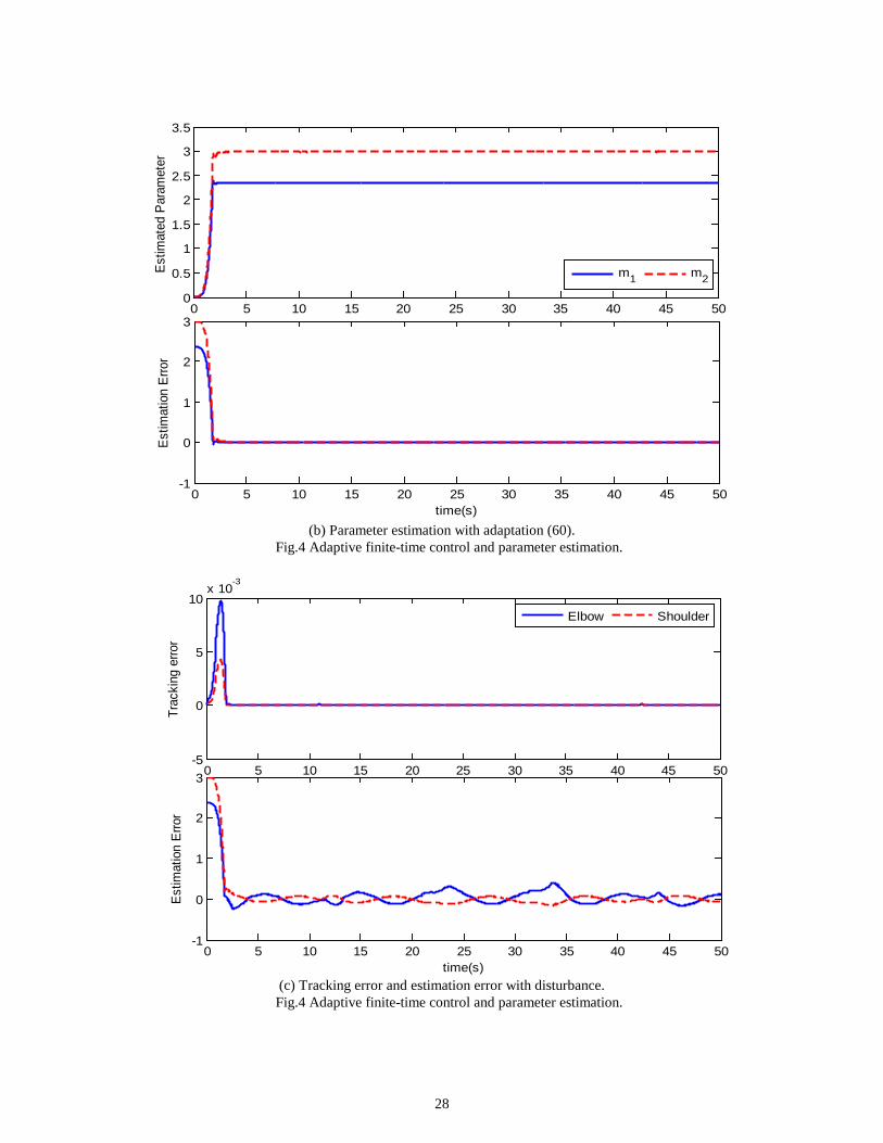
28

0 5 10 15 20 25 30 35 40 45 500

0.5

1

1.5

2

2.5

3

3.5

Estim

ated

Par

amet

er

m1 m2

0 5 10 15 20 25 30 35 40 45 50-1

0

1

2

3

time(s)

Estim

atio

n Er

ror

(b) Parameter estimation with adaptation (60).

Fig.4 Adaptive finite-time control and parameter estimation.

0 5 10 15 20 25 30 35 40 45 50-5

0

5

10x 10

-3

Trac

king

erro

r

Elbow Shoulder

0 5 10 15 20 25 30 35 40 45 50-1

0

1

2

3

time(s)

Estim

atio

n Er

ror

(c) Tracking error and estimation error with disturbance. Fig.4 Adaptive finite-time control and parameter estimation.