n t f v m ) be a es-net. any nontrivial integer solution x
TRANSCRIPT

7. Petri-Nets 7.4. Invariants Seite 100
Transition-Invariants (T-Invariants)
Let N = (P,T ,F ,V ,m0) be a eS-Net.
Any nontrivial integer solution x of the homogenous linear equation systemC · x = 0 is called transition-invariant (T-invariant) of N.
A T-invariant x is called proper, if x ≥ 0.
A T-invariant x is called realizable in N, if there exists a word q ∈W (T ) withq = x and a reachable marking m such that m[ q�m.
N is called covered with T-invariants, if there exists a T-invariant x of N with allcomponents positive, i.e. greater than 0.
Proper T-invariants denote possible cycles of the reachability graph - realizableT-invariants denote cycles which indeed may occur.
Distributed Systems Part 2 Transactional Distributed Systems Dr.-Ing. Thomas Hornung

7. Petri-Nets 7.4. Invariants Seite 101
Transition-Invariants (T-Invariants)
Let N = (P,T ,F ,V ,m0) be a eS-Net.
Any nontrivial integer solution x of the homogenous linear equation systemC · x = 0 is called transition-invariant (T-invariant) of N.
A T-invariant x is called proper, if x ≥ 0.
A T-invariant x is called realizable in N, if there exists a word q ∈W (T ) withq = x and a reachable marking m such that m[ q�m.
N is called covered with T-invariants, if there exists a T-invariant x of N with allcomponents positive, i.e. greater than 0.
Proper T-invariants denote possible cycles of the reachability graph - realizableT-invariants denote cycles which indeed may occur.
Distributed Systems Part 2 Transactional Distributed Systems Dr.-Ing. Thomas Hornung

7. Petri-Nets 7.4. Invariants Seite 102
Transition-Invariants (T-Invariants)
Let N = (P,T ,F ,V ,m0) be a eS-Net.
Any nontrivial integer solution x of the homogenous linear equation systemC · x = 0 is called transition-invariant (T-invariant) of N.
A T-invariant x is called proper, if x ≥ 0.
A T-invariant x is called realizable in N, if there exists a word q ∈W (T ) withq = x and a reachable marking m such that m[ q�m.
N is called covered with T-invariants, if there exists a T-invariant x of N with allcomponents positive, i.e. greater than 0.
Proper T-invariants denote possible cycles of the reachability graph - realizableT-invariants denote cycles which indeed may occur.
Distributed Systems Part 2 Transactional Distributed Systems Dr.-Ing. Thomas Hornung

7. Petri-Nets 7.4. Invariants Seite 103
Transition-Invariants (T-Invariants)
Let N = (P,T ,F ,V ,m0) be a eS-Net.
Any nontrivial integer solution x of the homogenous linear equation systemC · x = 0 is called transition-invariant (T-invariant) of N.
A T-invariant x is called proper, if x ≥ 0.
A T-invariant x is called realizable in N, if there exists a word q ∈W (T ) withq = x and a reachable marking m such that m[ q�m.
N is called covered with T-invariants, if there exists a T-invariant x of N with allcomponents positive, i.e. greater than 0.
Proper T-invariants denote possible cycles of the reachability graph - realizableT-invariants denote cycles which indeed may occur.
Distributed Systems Part 2 Transactional Distributed Systems Dr.-Ing. Thomas Hornung
7. Petri-Nets 7.4. Invariants Seite 104
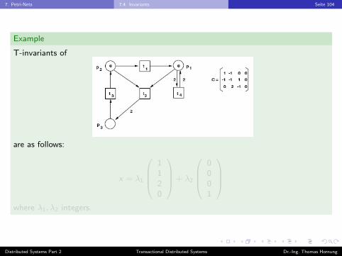
Example
T-invariants of
are as follows:
x = λ1
1120
+ λ2
0001
where λ1, λ2 integers.
Distributed Systems Part 2 Transactional Distributed Systems Dr.-Ing. Thomas Hornung
7. Petri-Nets 7.4. Invariants Seite 105
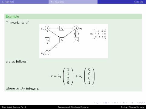
Example
T-invariants of
are as follows:
x = λ1
1120
+ λ2
0001
where λ1, λ2 integers.
Distributed Systems Part 2 Transactional Distributed Systems Dr.-Ing. Thomas Hornung

7. Petri-Nets 7.4. Invariants Seite 106
Theorem
Let N = (S ,T ,F ,V ,m0) be a eS-Net. If there exists a marking m, such that N liveand bounded at m, then N covered by T-invariants.
Proof: Let N live and bounded at some m.
As N is live at m, there exists a word q1 ∈ LN(m), which contains all transitions in T and themarking m + ∆q1 is reachable from m.
Moreover, N is live at m + ∆q1 as well. Therefore, there exits a word q2 ∈ LN(m), whichcontains all transitions in T and N is live at the marking m + ∆q1q2.
There exists an infinite sequence of markings (mi ), where mi := m + ∆q1 . . . qi , such that:
m[ q1�m1[ q2�m2 . . .mi [ qi+1�mi+1 . . .
As N is bounded at m, there is only a finite number of markings which are reachable.Therefore, there exist i , j ∈ NAT : i < j such that mi = mj . Thus
mi [ qi+1 . . . qj �mj = mi
As all these qi mention all transitions, we finally conclude
x = qi+1 + . . .+ qj
is a T-Invariant which covers N.
Distributed Systems Part 2 Transactional Distributed Systems Dr.-Ing. Thomas Hornung

7. Petri-Nets 7.4. Invariants Seite 107
Theorem
Let N = (S ,T ,F ,V ,m0) be a eS-Net. If there exists a marking m, such that N liveand bounded at m, then N covered by T-invariants.
Proof: Let N live and bounded at some m.
As N is live at m, there exists a word q1 ∈ LN(m), which contains all transitions in T and themarking m + ∆q1 is reachable from m.
Moreover, N is live at m + ∆q1 as well. Therefore, there exits a word q2 ∈ LN(m), whichcontains all transitions in T and N is live at the marking m + ∆q1q2.
There exists an infinite sequence of markings (mi ), where mi := m + ∆q1 . . . qi , such that:
m[ q1�m1[ q2�m2 . . .mi [ qi+1�mi+1 . . .
As N is bounded at m, there is only a finite number of markings which are reachable.Therefore, there exist i , j ∈ NAT : i < j such that mi = mj . Thus
mi [ qi+1 . . . qj �mj = mi
As all these qi mention all transitions, we finally conclude
x = qi+1 + . . .+ qj
is a T-Invariant which covers N.
Distributed Systems Part 2 Transactional Distributed Systems Dr.-Ing. Thomas Hornung

7. Petri-Nets 7.4. Invariants Seite 108
Theorem
Let N = (S ,T ,F ,V ,m0) be a eS-Net. If there exists a marking m, such that N liveand bounded at m, then N covered by T-invariants.
Proof: Let N live and bounded at some m.
As N is live at m, there exists a word q1 ∈ LN(m), which contains all transitions in T and themarking m + ∆q1 is reachable from m.
Moreover, N is live at m + ∆q1 as well. Therefore, there exits a word q2 ∈ LN(m), whichcontains all transitions in T and N is live at the marking m + ∆q1q2.
There exists an infinite sequence of markings (mi ), where mi := m + ∆q1 . . . qi , such that:
m[ q1�m1[ q2�m2 . . .mi [ qi+1�mi+1 . . .
As N is bounded at m, there is only a finite number of markings which are reachable.Therefore, there exist i , j ∈ NAT : i < j such that mi = mj . Thus
mi [ qi+1 . . . qj �mj = mi
As all these qi mention all transitions, we finally conclude
x = qi+1 + . . .+ qj
is a T-Invariant which covers N.
Distributed Systems Part 2 Transactional Distributed Systems Dr.-Ing. Thomas Hornung

7. Petri-Nets 7.4. Invariants Seite 109
Theorem
Let N = (S ,T ,F ,V ,m0) be a eS-Net. If there exists a marking m, such that N liveand bounded at m, then N covered by T-invariants.
Proof: Let N live and bounded at some m.
As N is live at m, there exists a word q1 ∈ LN(m), which contains all transitions in T and themarking m + ∆q1 is reachable from m.
Moreover, N is live at m + ∆q1 as well. Therefore, there exits a word q2 ∈ LN(m), whichcontains all transitions in T and N is live at the marking m + ∆q1q2.
There exists an infinite sequence of markings (mi ), where mi := m + ∆q1 . . . qi , such that:
m[ q1�m1[ q2�m2 . . .mi [ qi+1�mi+1 . . .
As N is bounded at m, there is only a finite number of markings which are reachable.Therefore, there exist i , j ∈ NAT : i < j such that mi = mj . Thus
mi [ qi+1 . . . qj �mj = mi
As all these qi mention all transitions, we finally conclude
x = qi+1 + . . .+ qj
is a T-Invariant which covers N.
Distributed Systems Part 2 Transactional Distributed Systems Dr.-Ing. Thomas Hornung

7. Petri-Nets 7.4. Invariants Seite 110
Theorem
Let N = (S ,T ,F ,V ,m0) be a eS-Net. If there exists a marking m, such that N liveand bounded at m, then N covered by T-invariants.
Proof: Let N live and bounded at some m.
As N is live at m, there exists a word q1 ∈ LN(m), which contains all transitions in T and themarking m + ∆q1 is reachable from m.
Moreover, N is live at m + ∆q1 as well. Therefore, there exits a word q2 ∈ LN(m), whichcontains all transitions in T and N is live at the marking m + ∆q1q2.
There exists an infinite sequence of markings (mi ), where mi := m + ∆q1 . . . qi , such that:
m[ q1�m1[ q2�m2 . . .mi [ qi+1�mi+1 . . .
As N is bounded at m, there is only a finite number of markings which are reachable.Therefore, there exist i , j ∈ NAT : i < j such that mi = mj . Thus
mi [ qi+1 . . . qj �mj = mi
As all these qi mention all transitions, we finally conclude
x = qi+1 + . . .+ qj
is a T-Invariant which covers N.
Distributed Systems Part 2 Transactional Distributed Systems Dr.-Ing. Thomas Hornung

7. Petri-Nets 7.4. Invariants Seite 111
Theorem
Let N = (S ,T ,F ,V ,m0) be a eS-Net. If there exists a marking m, such that N liveand bounded at m, then N covered by T-invariants.
Proof: Let N live and bounded at some m.
As N is live at m, there exists a word q1 ∈ LN(m), which contains all transitions in T and themarking m + ∆q1 is reachable from m.
Moreover, N is live at m + ∆q1 as well. Therefore, there exits a word q2 ∈ LN(m), whichcontains all transitions in T and N is live at the marking m + ∆q1q2.
There exists an infinite sequence of markings (mi ), where mi := m + ∆q1 . . . qi , such that:
m[ q1�m1[ q2�m2 . . .mi [ qi+1�mi+1 . . .
As N is bounded at m, there is only a finite number of markings which are reachable.Therefore, there exist i , j ∈ NAT : i < j such that mi = mj . Thus
mi [ qi+1 . . . qj �mj = mi
As all these qi mention all transitions, we finally conclude
x = qi+1 + . . .+ qj
is a T-Invariant which covers N.
Distributed Systems Part 2 Transactional Distributed Systems Dr.-Ing. Thomas Hornung

7. Petri-Nets 7.4. Invariants Seite 112
Useful application of the theorem:
Whenever N is not covered by T-invariants, then for every marking it holds N not liveor not bounded.
Distributed Systems Part 2 Transactional Distributed Systems Dr.-Ing. Thomas Hornung

7. Petri-Nets 7.4. Invariants Seite 113
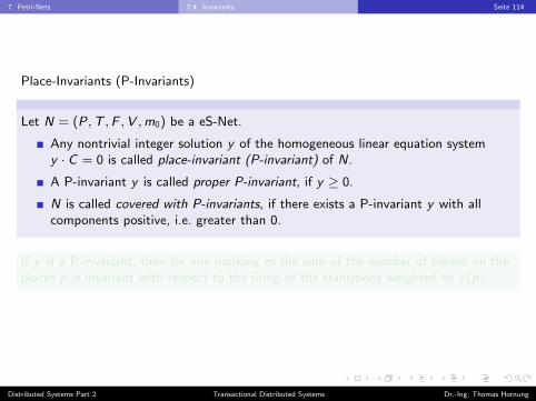
Place-Invariants (P-Invariants)
Let N = (P,T ,F ,V ,m0) be a eS-Net.
Any nontrivial integer solution y of the homogeneous linear equation systemy · C = 0 is called place-invariant (P-invariant) of N.
A P-invariant y is called proper P-invariant, if y ≥ 0.
N is called covered with P-invariants, if there exists a P-invariant y with allcomponents positive, i.e. greater than 0.
If y is a P-invariant, then for any marking m the sum of the number of tokens on theplaces p is invariant with respect to the firing of the transitions weighted by y(p).
Distributed Systems Part 2 Transactional Distributed Systems Dr.-Ing. Thomas Hornung
7. Petri-Nets 7.4. Invariants Seite 114
Place-Invariants (P-Invariants)
Let N = (P,T ,F ,V ,m0) be a eS-Net.
Any nontrivial integer solution y of the homogeneous linear equation systemy · C = 0 is called place-invariant (P-invariant) of N.
A P-invariant y is called proper P-invariant, if y ≥ 0.
N is called covered with P-invariants, if there exists a P-invariant y with allcomponents positive, i.e. greater than 0.
If y is a P-invariant, then for any marking m the sum of the number of tokens on theplaces p is invariant with respect to the firing of the transitions weighted by y(p).
Distributed Systems Part 2 Transactional Distributed Systems Dr.-Ing. Thomas Hornung

7. Petri-Nets 7.4. Invariants Seite 115
Place-Invariants (P-Invariants)
Let N = (P,T ,F ,V ,m0) be a eS-Net.
Any nontrivial integer solution y of the homogeneous linear equation systemy · C = 0 is called place-invariant (P-invariant) of N.
A P-invariant y is called proper P-invariant, if y ≥ 0.
N is called covered with P-invariants, if there exists a P-invariant y with allcomponents positive, i.e. greater than 0.
If y is a P-invariant, then for any marking m the sum of the number of tokens on theplaces p is invariant with respect to the firing of the transitions weighted by y(p).
Distributed Systems Part 2 Transactional Distributed Systems Dr.-Ing. Thomas Hornung
7. Petri-Nets 7.4. Invariants Seite 116
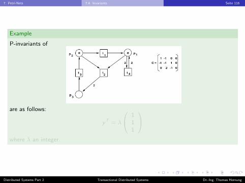
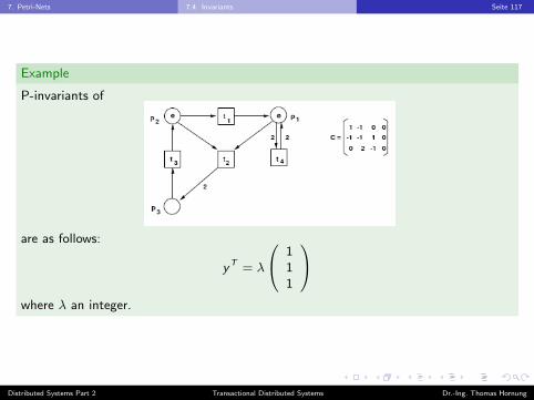
Example
P-invariants of
are as follows:
yT = λ
111
where λ an integer.
Distributed Systems Part 2 Transactional Distributed Systems Dr.-Ing. Thomas Hornung
7. Petri-Nets 7.4. Invariants Seite 117
Example
P-invariants of
are as follows:
yT = λ
111
where λ an integer.
Distributed Systems Part 2 Transactional Distributed Systems Dr.-Ing. Thomas Hornung

7. Petri-Nets 7.4. Invariants Seite 118
Theorem
Let N = (P,T ,F ,V ,m0) a eS-Net and let y a P-invariant of N. Then:
m ∈ RN(m0)⇒ y ·m> = y ·m>0 .
Proof:Assume m0[ q�m. Then m = m0 + (C · q)> and also:
y ·m> = y ·m>0 + y · (C · q) =
= y ·m>0 + (y · C) · q = y ·m>0 + 0 · q = y ·m>0 .
Distributed Systems Part 2 Transactional Distributed Systems Dr.-Ing. Thomas Hornung

7. Petri-Nets 7.4. Invariants Seite 119
Theorem
Let N = (P,T ,F ,V ,m0) a eS-Net and let y a P-invariant of N. Then:
m ∈ RN(m0)⇒ y ·m> = y ·m>0 .
Proof:Assume m0[ q�m. Then m = m0 + (C · q)> and also:
y ·m> = y ·m>0 + y · (C · q) =
= y ·m>0 + (y · C) · q = y ·m>0 + 0 · q = y ·m>0 .
Distributed Systems Part 2 Transactional Distributed Systems Dr.-Ing. Thomas Hornung

7. Petri-Nets 7.4. Invariants Seite 120
Corollary:
Let y P-invariante of N, m marking.
y ·m> 6= y ·m>0 ⇒ m 6∈ RN(m0).
Let y proper P-invariant of N. Let p ∈ P such that y(p) > 0.
Then, for any initial marking, p is bounded.
Proof: y ·m>0 = y ·m> ≥ y(p) ·m(p) ≥ m(p).
Let N be covered by P-invariants. N is bounded for any initial marking.
Distributed Systems Part 2 Transactional Distributed Systems Dr.-Ing. Thomas Hornung

7. Petri-Nets 7.4. Invariants Seite 121
Corollary:
Let y P-invariante of N, m marking.
y ·m> 6= y ·m>0 ⇒ m 6∈ RN(m0).
Let y proper P-invariant of N. Let p ∈ P such that y(p) > 0.
Then, for any initial marking, p is bounded.
Proof: y ·m>0 = y ·m> ≥ y(p) ·m(p) ≥ m(p).
Let N be covered by P-invariants. N is bounded for any initial marking.
Distributed Systems Part 2 Transactional Distributed Systems Dr.-Ing. Thomas Hornung

7. Petri-Nets 7.4. Invariants Seite 122
Corollary:
Let y P-invariante of N, m marking.
y ·m> 6= y ·m>0 ⇒ m 6∈ RN(m0).
Let y proper P-invariant of N. Let p ∈ P such that y(p) > 0.
Then, for any initial marking, p is bounded.
Proof: y ·m>0 = y ·m> ≥ y(p) ·m(p) ≥ m(p).
Let N be covered by P-invariants. N is bounded for any initial marking.
Distributed Systems Part 2 Transactional Distributed Systems Dr.-Ing. Thomas Hornung

7. Petri-Nets 7.4. Invariants Seite 123
Note, the following net is bounded for any initial marking, however does not have aP-invariant:
P-invariants allow sufficient tests for non-reachability and boundedeness.
Distributed Systems Part 2 Transactional Distributed Systems Dr.-Ing. Thomas Hornung

7. Petri-Nets 7.4. Invariants Seite 124
Note, the following net is bounded for any initial marking, however does not have aP-invariant:
P-invariants allow sufficient tests for non-reachability and boundedeness.
Distributed Systems Part 2 Transactional Distributed Systems Dr.-Ing. Thomas Hornung
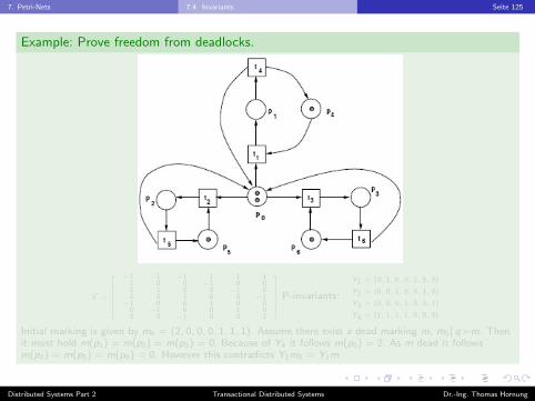
7. Petri-Nets 7.4. Invariants Seite 125
Example: Prove freedom from deadlocks.
C =
−1 −1 −1 1 1 11 0 0 −1 0 00 1 0 0 −1 00 0 1 0 0 −1−1 0 0 1 0 0
0 −1 0 0 1 00 0 −1 0 0 1
P-invariants:
Y1 = (0, 1, 0, 0, 1, 0, 0)
Y2 = (0, 0, 1, 0, 0, 1, 0)
Y3 = (0, 0, 0, 1, 0, 0, 1)
Y4 = (1, 1, 1, 1, 0, 0, 0)
Initial marking is given by m0 = (2, 0, 0, 0, 1, 1, 1). Assume there exist a dead marking m, m0[ q�m. Thenit must hold m(p1) = m(p2) = m(p3) = 0. Because of Y4 it follows m(p0) = 2. As m dead it followsm(p4) = m(p5) = m(p6) = 0. However this contradicts Y1m0 = Y1m.
Distributed Systems Part 2 Transactional Distributed Systems Dr.-Ing. Thomas Hornung

7. Petri-Nets 7.4. Invariants Seite 126
Example: Prove freedom from deadlocks.
C =
−1 −1 −1 1 1 11 0 0 −1 0 00 1 0 0 −1 00 0 1 0 0 −1−1 0 0 1 0 0
0 −1 0 0 1 00 0 −1 0 0 1
P-invariants:
Y1 = (0, 1, 0, 0, 1, 0, 0)
Y2 = (0, 0, 1, 0, 0, 1, 0)
Y3 = (0, 0, 0, 1, 0, 0, 1)
Y4 = (1, 1, 1, 1, 0, 0, 0)
Initial marking is given by m0 = (2, 0, 0, 0, 1, 1, 1). Assume there exist a dead marking m, m0[ q�m. Thenit must hold m(p1) = m(p2) = m(p3) = 0. Because of Y4 it follows m(p0) = 2. As m dead it followsm(p4) = m(p5) = m(p6) = 0. However this contradicts Y1m0 = Y1m.
Distributed Systems Part 2 Transactional Distributed Systems Dr.-Ing. Thomas Hornung

7. Petri-Nets 7.4. Invariants Seite 127
Example: Prove freedom from deadlocks.
C =
−1 −1 −1 1 1 11 0 0 −1 0 00 1 0 0 −1 00 0 1 0 0 −1−1 0 0 1 0 0
0 −1 0 0 1 00 0 −1 0 0 1
P-invariants:
Y1 = (0, 1, 0, 0, 1, 0, 0)
Y2 = (0, 0, 1, 0, 0, 1, 0)
Y3 = (0, 0, 0, 1, 0, 0, 1)
Y4 = (1, 1, 1, 1, 0, 0, 0)
Initial marking is given by m0 = (2, 0, 0, 0, 1, 1, 1). Assume there exist a dead marking m, m0[ q�m. Thenit must hold m(p1) = m(p2) = m(p3) = 0. Because of Y4 it follows m(p0) = 2. As m dead it followsm(p4) = m(p5) = m(p6) = 0. However this contradicts Y1m0 = Y1m.
Distributed Systems Part 2 Transactional Distributed Systems Dr.-Ing. Thomas Hornung

7. Petri-Nets 7.5. Place Capacities Seite 128
Section 7.5 Place Capacities
Sometimes when modelling we would like to fix an upper bound for the number oftokens in a place.
Let N = (P,T ,F ,V ,m0) be a eS-Net, c a ω-marking of P and let m0 ≤ c.(N, c) is called eS-Net with capacities. c(p), p ∈ P is called capacity of p.
For eS-nets with capacities the notion of being enabled is adapted:
a transition t ∈ T is enabled at marking m, if t− ≤ m andm + ∆t ≤ c.
Capacities graphically are labels of places - no label means capacity ω.
Distributed Systems Part 2 Transactional Distributed Systems Dr.-Ing. Thomas Hornung

7. Petri-Nets 7.5. Place Capacities Seite 129
Section 7.5 Place Capacities
Sometimes when modelling we would like to fix an upper bound for the number oftokens in a place.
Let N = (P,T ,F ,V ,m0) be a eS-Net, c a ω-marking of P and let m0 ≤ c.(N, c) is called eS-Net with capacities. c(p), p ∈ P is called capacity of p.
For eS-nets with capacities the notion of being enabled is adapted:
a transition t ∈ T is enabled at marking m, if t− ≤ m andm + ∆t ≤ c.
Capacities graphically are labels of places - no label means capacity ω.
Distributed Systems Part 2 Transactional Distributed Systems Dr.-Ing. Thomas Hornung

7. Petri-Nets 7.5. Place Capacities Seite 130
Section 7.5 Place Capacities
Sometimes when modelling we would like to fix an upper bound for the number oftokens in a place.
Let N = (P,T ,F ,V ,m0) be a eS-Net, c a ω-marking of P and let m0 ≤ c.(N, c) is called eS-Net with capacities. c(p), p ∈ P is called capacity of p.
For eS-nets with capacities the notion of being enabled is adapted:
a transition t ∈ T is enabled at marking m, if t− ≤ m andm + ∆t ≤ c.
Capacities graphically are labels of places - no label means capacity ω.
Distributed Systems Part 2 Transactional Distributed Systems Dr.-Ing. Thomas Hornung

7. Petri-Nets 7.5. Place Capacities Seite 131
Section 7.5 Place Capacities
Sometimes when modelling we would like to fix an upper bound for the number oftokens in a place.
Let N = (P,T ,F ,V ,m0) be a eS-Net, c a ω-marking of P and let m0 ≤ c.(N, c) is called eS-Net with capacities. c(p), p ∈ P is called capacity of p.
For eS-nets with capacities the notion of being enabled is adapted:
a transition t ∈ T is enabled at marking m, if t− ≤ m andm + ∆t ≤ c.
Capacities graphically are labels of places - no label means capacity ω.
Distributed Systems Part 2 Transactional Distributed Systems Dr.-Ing. Thomas Hornung

7. Petri-Nets 7.5. Place Capacities Seite 132
Any eS-net with capacities can be simulated by a eS-Net without capacities.
Construction
Let p a palce with capacity k = c(p), k ≥ 1. Let pco be the complementary placeof p which is assigned the initial marking k −m0(p).
Whenever for a transition t we have ∆t(p) > 0, we introduce an arc from pco tot with multiplicity ∆t(p);whenever ∆t(p) < 0, we introduce an arc from t to pco with multiplicity −∆t(p).
Distributed Systems Part 2 Transactional Distributed Systems Dr.-Ing. Thomas Hornung

7. Petri-Nets 7.5. Place Capacities Seite 133
Any eS-net with capacities can be simulated by a eS-Net without capacities.
Construction
Let p a palce with capacity k = c(p), k ≥ 1. Let pco be the complementary placeof p which is assigned the initial marking k −m0(p).
Whenever for a transition t we have ∆t(p) > 0, we introduce an arc from pco tot with multiplicity ∆t(p);whenever ∆t(p) < 0, we introduce an arc from t to pco with multiplicity −∆t(p).
Distributed Systems Part 2 Transactional Distributed Systems Dr.-Ing. Thomas Hornung

7. Petri-Nets 7.5. Place Capacities Seite 134
Any eS-net with capacities can be simulated by a eS-Net without capacities.
Construction
Let p a palce with capacity k = c(p), k ≥ 1. Let pco be the complementary placeof p which is assigned the initial marking k −m0(p).
Whenever for a transition t we have ∆t(p) > 0, we introduce an arc from pco tot with multiplicity ∆t(p);whenever ∆t(p) < 0, we introduce an arc from t to pco with multiplicity −∆t(p).
Distributed Systems Part 2 Transactional Distributed Systems Dr.-Ing. Thomas Hornung

7. Petri-Nets 7.5. Place Capacities Seite 135
A eS-Net with capacities and its simulation by a bounded eS-Net.
Distributed Systems Part 2 Transactional Distributed Systems Dr.-Ing. Thomas Hornung

7. Petri-Nets 7.6. S-Nets with Colors Seite 136
Section 7.6 S-Nets with Colors
eS-Nets in practice may become huge and difficult to understand.
Sometimes such nets exhibit certain regularities which give rise to questions howto reduce the size of the net without losing modeling properties.
Distributed Systems Part 2 Transactional Distributed Systems Dr.-Ing. Thomas Hornung

7. Petri-Nets 7.6. S-Nets with Colors Seite 137
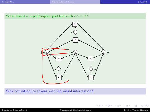
What about a n-philosopher problem with n >> 3?
i 1
b 2
e2
e3
b 3
b 1
e1
i 2 i 3
g 1 g 2 g 3
i 1
b 2
e2
e3
b 3
b 1
e1
i 2 i 3
g 1 g 2 g 3
i 1
b 2
e2
e3
b 3
b 1
e1
i 2 i 3
g 1 g 2 g 3
Why not introduce tokens with individual information?
Distributed Systems Part 2 Transactional Distributed Systems Dr.-Ing. Thomas Hornung
7. Petri-Nets 7.6. S-Nets with Colors Seite 138
What about a n-philosopher problem with n >> 3?
i 1
b 2
e2
e3
b 3
b 1
e1
i 2 i 3
g 1 g 2 g 3
i 1
b 2
e2
e3
b 3
b 1
e1
i 2 i 3
g 1 g 2 g 3
i 1
b 2
e2
e3
b 3
b 1
e1
i 2 i 3
g 1 g 2 g 3
Why not introduce tokens with individual information?
Distributed Systems Part 2 Transactional Distributed Systems Dr.-Ing. Thomas Hornung

7. Petri-Nets 7.6. S-Nets with Colors Seite 139
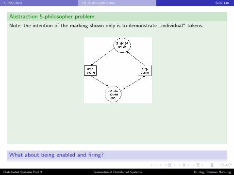
Abstraction 5-philosopher problem
Note: the intention of the marking shown only is to demonstrate”individual“ tokens.
What about being enabled and firing?
Distributed Systems Part 2 Transactional Distributed Systems Dr.-Ing. Thomas Hornung
7. Petri-Nets 7.6. S-Nets with Colors Seite 140
Abstraction 5-philosopher problem
Note: the intention of the marking shown only is to demonstrate”individual“ tokens.
What about being enabled and firing?
Distributed Systems Part 2 Transactional Distributed Systems Dr.-Ing. Thomas Hornung

7. Petri-Nets 7.6. S-Nets with Colors Seite 141
Colored System-Nets
A colored System-Net distinguishes different kinds of sorts for markings - the so calledcolors - and functions over these sorts which are used to label the edges of the net.
Generalizing eS-Nets, in a colored net a transition will be called enabled, if certainconditions are true, which are based on the functions which are assigned to the edgesof the transitions surrounding.
Thus, we have colors, to characterize markings (place colors), and colors, tocharacterize the firing of transitions (transition colors).
As a marking of a place now can be built out of different kind of tokens, we introducemultisets.
Let A be a set. A multiset m over A is given by a maping m : A→ NAT .
Let a ∈ A. If m[a] = k then there exist k occurences of a in m.
A multiset oftenly is written as a (formal) sum, e.g. [Apple,Apple,Pear ] iswritten as 2 · Apple + 1 · Pear .
Distributed Systems Part 2 Transactional Distributed Systems Dr.-Ing. Thomas Hornung

7. Petri-Nets 7.6. S-Nets with Colors Seite 142
Colored System-Nets
A colored System-Net distinguishes different kinds of sorts for markings - the so calledcolors - and functions over these sorts which are used to label the edges of the net.
Generalizing eS-Nets, in a colored net a transition will be called enabled, if certainconditions are true, which are based on the functions which are assigned to the edgesof the transitions surrounding.
Thus, we have colors, to characterize markings (place colors), and colors, tocharacterize the firing of transitions (transition colors).
As a marking of a place now can be built out of different kind of tokens, we introducemultisets.
Let A be a set. A multiset m over A is given by a maping m : A→ NAT .
Let a ∈ A. If m[a] = k then there exist k occurences of a in m.
A multiset oftenly is written as a (formal) sum, e.g. [Apple,Apple,Pear ] iswritten as 2 · Apple + 1 · Pear .
Distributed Systems Part 2 Transactional Distributed Systems Dr.-Ing. Thomas Hornung

7. Petri-Nets 7.6. S-Nets with Colors Seite 143
Colored System-Nets
A colored System-Net distinguishes different kinds of sorts for markings - the so calledcolors - and functions over these sorts which are used to label the edges of the net.
Generalizing eS-Nets, in a colored net a transition will be called enabled, if certainconditions are true, which are based on the functions which are assigned to the edgesof the transitions surrounding.
Thus, we have colors, to characterize markings (place colors), and colors, tocharacterize the firing of transitions (transition colors).
As a marking of a place now can be built out of different kind of tokens, we introducemultisets.
Let A be a set. A multiset m over A is given by a maping m : A→ NAT .
Let a ∈ A. If m[a] = k then there exist k occurences of a in m.
A multiset oftenly is written as a (formal) sum, e.g. [Apple,Apple,Pear ] iswritten as 2 · Apple + 1 · Pear .
Distributed Systems Part 2 Transactional Distributed Systems Dr.-Ing. Thomas Hornung

7. Petri-Nets 7.6. S-Nets with Colors Seite 144
Colored System-Nets
A colored System-Net distinguishes different kinds of sorts for markings - the so calledcolors - and functions over these sorts which are used to label the edges of the net.
Generalizing eS-Nets, in a colored net a transition will be called enabled, if certainconditions are true, which are based on the functions which are assigned to the edgesof the transitions surrounding.
Thus, we have colors, to characterize markings (place colors), and colors, tocharacterize the firing of transitions (transition colors).
As a marking of a place now can be built out of different kind of tokens, we introducemultisets.
Let A be a set. A multiset m over A is given by a maping m : A→ NAT .
Let a ∈ A. If m[a] = k then there exist k occurences of a in m.
A multiset oftenly is written as a (formal) sum, e.g. [Apple,Apple,Pear ] iswritten as 2 · Apple + 1 · Pear .
Distributed Systems Part 2 Transactional Distributed Systems Dr.-Ing. Thomas Hornung

7. Petri-Nets 7.6. S-Nets with Colors Seite 145
Colored System-Nets
A colored System-Net distinguishes different kinds of sorts for markings - the so calledcolors - and functions over these sorts which are used to label the edges of the net.
Generalizing eS-Nets, in a colored net a transition will be called enabled, if certainconditions are true, which are based on the functions which are assigned to the edgesof the transitions surrounding.
Thus, we have colors, to characterize markings (place colors), and colors, tocharacterize the firing of transitions (transition colors).
As a marking of a place now can be built out of different kind of tokens, we introducemultisets.
Let A be a set. A multiset m over A is given by a maping m : A→ NAT .
Let a ∈ A. If m[a] = k then there exist k occurences of a in m.
A multiset oftenly is written as a (formal) sum, e.g. [Apple,Apple,Pear ] iswritten as 2 · Apple + 1 · Pear .
Distributed Systems Part 2 Transactional Distributed Systems Dr.-Ing. Thomas Hornung
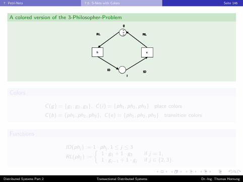
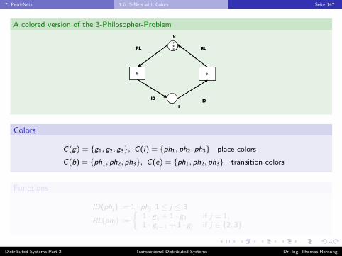
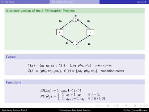
7. Petri-Nets 7.6. S-Nets with Colors Seite 146
A colored version of the 3-Philosopher-Problem
b e
ID
g
RL
g1
g2
g3 RL
IDi
b e
ID
g
RL
g1
g2
g3 RL
IDi
Colors
C(g) = {g1, g2, g3}, C(i) = {ph1, ph2, ph3} place colors
C(b) = {ph1, ph2, ph3}, C(e) = {ph1, ph2, ph3} transition colors
Functions
ID(phj ) := 1 · phj , 1 ≤ j ≤ 3
RL(phj ) :=
{1 · g1 + 1 · g3 if j = 1,1 · gj−1 + 1 · gj if j ∈ {2, 3}.
Distributed Systems Part 2 Transactional Distributed Systems Dr.-Ing. Thomas Hornung
7. Petri-Nets 7.6. S-Nets with Colors Seite 147
A colored version of the 3-Philosopher-Problem
b e
ID
g
RL
g1
g2
g3 RL
IDi
b e
ID
g
RL
g1
g2
g3 RL
IDi
Colors
C(g) = {g1, g2, g3}, C(i) = {ph1, ph2, ph3} place colors
C(b) = {ph1, ph2, ph3}, C(e) = {ph1, ph2, ph3} transition colors
Functions
ID(phj ) := 1 · phj , 1 ≤ j ≤ 3
RL(phj ) :=
{1 · g1 + 1 · g3 if j = 1,1 · gj−1 + 1 · gj if j ∈ {2, 3}.
Distributed Systems Part 2 Transactional Distributed Systems Dr.-Ing. Thomas Hornung
7. Petri-Nets 7.6. S-Nets with Colors Seite 148
A colored version of the 3-Philosopher-Problem
b e
ID
g
RL
g1
g2
g3 RL
IDi
b e
ID
g
RL
g1
g2
g3 RL
IDi
Colors
C(g) = {g1, g2, g3}, C(i) = {ph1, ph2, ph3} place colors
C(b) = {ph1, ph2, ph3}, C(e) = {ph1, ph2, ph3} transition colors
Functions
ID(phj ) := 1 · phj , 1 ≤ j ≤ 3
RL(phj ) :=
{1 · g1 + 1 · g3 if j = 1,1 · gj−1 + 1 · gj if j ∈ {2, 3}.
Distributed Systems Part 2 Transactional Distributed Systems Dr.-Ing. Thomas Hornung

7. Petri-Nets 7.6. S-Nets with Colors Seite 149
Multiplicities
A multiplicity assigned to an edge between a place p and a transition t is a mappingfrom the set of transition colors of t into the set of multisets over the colors of p.
In the example:
V (b, i) = V (i , e) = ID, V (g , b) = V (e, g) = RL,
where:ID(phj) := 1 · phj , 1 ≤ j ≤ 3
RL(phj) :=
{1 · g1 + 1 · g3 if j = 1,1 · gj−1 + 1 · gj if j ∈ {2, 3}.
ID denotes the identity mapping.
Marking
Markings are multisets over the respective place colors.
In the example:
m0(p) :=
{1 · g1 + 1 · g2 + 1 · g3 if p = g ,0 otherwise.
Distributed Systems Part 2 Transactional Distributed Systems Dr.-Ing. Thomas Hornung

7. Petri-Nets 7.6. S-Nets with Colors Seite 150
Multiplicities
A multiplicity assigned to an edge between a place p and a transition t is a mappingfrom the set of transition colors of t into the set of multisets over the colors of p.
In the example:
V (b, i) = V (i , e) = ID, V (g , b) = V (e, g) = RL,
where:ID(phj) := 1 · phj , 1 ≤ j ≤ 3
RL(phj) :=
{1 · g1 + 1 · g3 if j = 1,1 · gj−1 + 1 · gj if j ∈ {2, 3}.
ID denotes the identity mapping.
Marking
Markings are multisets over the respective place colors.
In the example:
m0(p) :=
{1 · g1 + 1 · g2 + 1 · g3 if p = g ,0 otherwise.
Distributed Systems Part 2 Transactional Distributed Systems Dr.-Ing. Thomas Hornung

7. Petri-Nets 7.6. S-Nets with Colors Seite 151
Multiplicities
A multiplicity assigned to an edge between a place p and a transition t is a mappingfrom the set of transition colors of t into the set of multisets over the colors of p.
In the example:
V (b, i) = V (i , e) = ID, V (g , b) = V (e, g) = RL,
where:ID(phj) := 1 · phj , 1 ≤ j ≤ 3
RL(phj) :=
{1 · g1 + 1 · g3 if j = 1,1 · gj−1 + 1 · gj if j ∈ {2, 3}.
ID denotes the identity mapping.
Marking
Markings are multisets over the respective place colors.
In the example:
m0(p) :=
{1 · g1 + 1 · g2 + 1 · g3 if p = g ,0 otherwise.
Distributed Systems Part 2 Transactional Distributed Systems Dr.-Ing. Thomas Hornung

7. Petri-Nets 7.6. S-Nets with Colors Seite 152
Multiplicities
A multiplicity assigned to an edge between a place p and a transition t is a mappingfrom the set of transition colors of t into the set of multisets over the colors of p.
In the example:
V (b, i) = V (i , e) = ID, V (g , b) = V (e, g) = RL,
where:ID(phj) := 1 · phj , 1 ≤ j ≤ 3
RL(phj) :=
{1 · g1 + 1 · g3 if j = 1,1 · gj−1 + 1 · gj if j ∈ {2, 3}.
ID denotes the identity mapping.
Marking
Markings are multisets over the respective place colors.
In the example:
m0(p) :=
{1 · g1 + 1 · g2 + 1 · g3 if p = g ,0 otherwise.
Distributed Systems Part 2 Transactional Distributed Systems Dr.-Ing. Thomas Hornung

7. Petri-Nets 7.6. S-Nets with Colors Seite 153
A colored Net CN = (P,T ,F ,C ,V ,m0) is given by:
A net (P,T ,F ).
A mapping C which assignes to each x ∈ P ∪ T a finite nonempty set C(x) ofcolors.
Mapping V assignes to each edge f ∈ F a mapping V (f ).
Let f be an edge connecting palce p and transition t.
V (f ) is a mapping from C(t) into the set of multisets over C(p).
m0 is the initial marking given by a mapping which assignes to each place p amultiset m0(p) over C(p).
Distributed Systems Part 2 Transactional Distributed Systems Dr.-Ing. Thomas Hornung

7. Petri-Nets 7.6. S-Nets with Colors Seite 154
A colored Net CN = (P,T ,F ,C ,V ,m0) is given by:
A net (P,T ,F ).
A mapping C which assignes to each x ∈ P ∪ T a finite nonempty set C(x) ofcolors.
Mapping V assignes to each edge f ∈ F a mapping V (f ).
Let f be an edge connecting palce p and transition t.
V (f ) is a mapping from C(t) into the set of multisets over C(p).
m0 is the initial marking given by a mapping which assignes to each place p amultiset m0(p) over C(p).
Distributed Systems Part 2 Transactional Distributed Systems Dr.-Ing. Thomas Hornung

7. Petri-Nets 7.6. S-Nets with Colors Seite 155
A colored Net CN = (P,T ,F ,C ,V ,m0) is given by:
A net (P,T ,F ).
A mapping C which assignes to each x ∈ P ∪ T a finite nonempty set C(x) ofcolors.
Mapping V assignes to each edge f ∈ F a mapping V (f ).
Let f be an edge connecting palce p and transition t.
V (f ) is a mapping from C(t) into the set of multisets over C(p).
m0 is the initial marking given by a mapping which assignes to each place p amultiset m0(p) over C(p).
Distributed Systems Part 2 Transactional Distributed Systems Dr.-Ing. Thomas Hornung

7. Petri-Nets 7.6. S-Nets with Colors Seite 156
A colored Net CN = (P,T ,F ,C ,V ,m0) is given by:
A net (P,T ,F ).
A mapping C which assignes to each x ∈ P ∪ T a finite nonempty set C(x) ofcolors.
Mapping V assignes to each edge f ∈ F a mapping V (f ).
Let f be an edge connecting palce p and transition t.
V (f ) is a mapping from C(t) into the set of multisets over C(p).
m0 is the initial marking given by a mapping which assignes to each place p amultiset m0(p) over C(p).
Distributed Systems Part 2 Transactional Distributed Systems Dr.-Ing. Thomas Hornung

7. Petri-Nets 7.6. S-Nets with Colors Seite 157
Let CN = (P,T ,F ,C ,V ,m0) be a colored System-Net.
A marking m of P is mapping which assignes to each place p a multiset m(p)over C(p).
A transition t is enabled in color d ∈ C(t) at m, if for all pre-places p ∈ Ft thereholds:
V (p, t)(d) ≤ m(p).
Assume t is enabled in color d at marking m. Firing of t in color d transforms mto a marking m′:
m′(p) :=
m(p)− V (p, t)(d) + V (t, p)(d) if p ∈ Ft,p ∈ tF ,
m(p)− V (p, t)(d) if p ∈ Ft,,p 6∈ tF ,
m(p) + V (t, p)(d) if p 6∈ Ft,,p ∈ tF ,
m(p) otherwise.
Distributed Systems Part 2 Transactional Distributed Systems Dr.-Ing. Thomas Hornung

7. Petri-Nets 7.6. S-Nets with Colors Seite 158
Let CN = (P,T ,F ,C ,V ,m0) be a colored System-Net.
A marking m of P is mapping which assignes to each place p a multiset m(p)over C(p).
A transition t is enabled in color d ∈ C(t) at m, if for all pre-places p ∈ Ft thereholds:
V (p, t)(d) ≤ m(p).
Assume t is enabled in color d at marking m. Firing of t in color d transforms mto a marking m′:
m′(p) :=
m(p)− V (p, t)(d) + V (t, p)(d) if p ∈ Ft,p ∈ tF ,
m(p)− V (p, t)(d) if p ∈ Ft,,p 6∈ tF ,
m(p) + V (t, p)(d) if p 6∈ Ft,,p ∈ tF ,
m(p) otherwise.
Distributed Systems Part 2 Transactional Distributed Systems Dr.-Ing. Thomas Hornung

7. Petri-Nets 7.6. S-Nets with Colors Seite 159
Let CN = (P,T ,F ,C ,V ,m0) be a colored System-Net.
A marking m of P is mapping which assignes to each place p a multiset m(p)over C(p).
A transition t is enabled in color d ∈ C(t) at m, if for all pre-places p ∈ Ft thereholds:
V (p, t)(d) ≤ m(p).
Assume t is enabled in color d at marking m. Firing of t in color d transforms mto a marking m′:
m′(p) :=
m(p)− V (p, t)(d) + V (t, p)(d) if p ∈ Ft,p ∈ tF ,
m(p)− V (p, t)(d) if p ∈ Ft,,p 6∈ tF ,
m(p) + V (t, p)(d) if p 6∈ Ft,,p ∈ tF ,
m(p) otherwise.
Distributed Systems Part 2 Transactional Distributed Systems Dr.-Ing. Thomas Hornung

7. Petri-Nets 7.6. S-Nets with Colors Seite 160
Fold and Unfold of a Colored System-Net
Folding
By folding of a eS-Net we can reduce the number of places and transitions; places andtransitions are represented by appropriate place and transition colors, on which certainfunctions defining the multiplicities are defined.
Let N = (P,T ,F ,V ,m0) a eS-Net. A folding is defined by π and τ :
π = {q1, . . . , qk} a (disjoint) partition of P,
τ = {u1, . . . , un} a (disjoint) partition of T .
Distributed Systems Part 2 Transactional Distributed Systems Dr.-Ing. Thomas Hornung

7. Petri-Nets 7.6. S-Nets with Colors Seite 161
Fold and Unfold of a Colored System-Net
Folding
By folding of a eS-Net we can reduce the number of places and transitions; places andtransitions are represented by appropriate place and transition colors, on which certainfunctions defining the multiplicities are defined.
Let N = (P,T ,F ,V ,m0) a eS-Net. A folding is defined by π and τ :
π = {q1, . . . , qk} a (disjoint) partition of P,
τ = {u1, . . . , un} a (disjoint) partition of T .
Distributed Systems Part 2 Transactional Distributed Systems Dr.-Ing. Thomas Hornung

7. Petri-Nets 7.6. S-Nets with Colors Seite 162
Two special cases
Call GN(π, τ) := (P ′,T ′,F ′,C ′,V ′,m′0) the result of folding.
All elements of π, τ are one-elementary:
⇒ N and GN(π, τ) are isomorph,
π, τ contain only one element:
⇒ |P ′| = |T ′| = 1, ”the model is represented by the labellings”.
Distributed Systems Part 2 Transactional Distributed Systems Dr.-Ing. Thomas Hornung

7. Petri-Nets 7.6. S-Nets with Colors Seite 163
Two special cases
Call GN(π, τ) := (P ′,T ′,F ′,C ′,V ′,m′0) the result of folding.
All elements of π, τ are one-elementary:
⇒ N and GN(π, τ) are isomorph,
π, τ contain only one element:
⇒ |P ′| = |T ′| = 1, ”the model is represented by the labellings”.
Distributed Systems Part 2 Transactional Distributed Systems Dr.-Ing. Thomas Hornung
7. Petri-Nets 7.6. S-Nets with Colors Seite 164
Two special cases
Call GN(π, τ) := (P ′,T ′,F ′,C ′,V ′,m′0) the result of folding.
All elements of π, τ are one-elementary:
⇒ N and GN(π, τ) are isomorph,
π, τ contain only one element:
⇒ |P ′| = |T ′| = 1, ”the model is represented by the labellings”.
Distributed Systems Part 2 Transactional Distributed Systems Dr.-Ing. Thomas Hornung

7. Petri-Nets 7.6. S-Nets with Colors Seite 165
3-Philosopher-Problem
i 1
b 2
e2
e3
b 3
b 1
e1
i 2 i 3
g 1 g 2 g 3
i 1
b 2
e2
e3
b 3
b 1
e1
i 2 i 3
g 1 g 2 g 3
i 1
b 2
e2
e3
b 3
b 1
e1
i 2 i 3
g 1 g 2 g 3
Folding π = {{g1, g2, g3}, {i1, i2, i3}}, τ = {{b1, b2, b3}, {e1, e2, e3}}.
Colors from folding:C(g) = {g1, g2, g3},C(i) = {i1, i2, i3},C(b) = {b1, b2, b3},C(e) = {e1, e2, e3}
Multiplicities: ID,RL analogously to previous version.
b e
ID
g
RL
g1
g2
g3 RL
IDi
b e
ID
g
RL
g1
g2
g3 RL
IDi
Distributed Systems Part 2 Transactional Distributed Systems Dr.-Ing. Thomas Hornung
7. Petri-Nets 7.6. S-Nets with Colors Seite 166
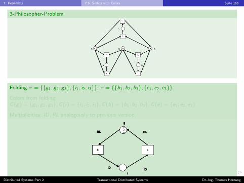
3-Philosopher-Problem
i 1
b 2
e2
e3
b 3
b 1
e1
i 2 i 3
g 1 g 2 g 3
i 1
b 2
e2
e3
b 3
b 1
e1
i 2 i 3
g 1 g 2 g 3
i 1
b 2
e2
e3
b 3
b 1
e1
i 2 i 3
g 1 g 2 g 3
Folding π = {{g1, g2, g3}, {i1, i2, i3}}, τ = {{b1, b2, b3}, {e1, e2, e3}}.
Colors from folding:C(g) = {g1, g2, g3},C(i) = {i1, i2, i3},C(b) = {b1, b2, b3},C(e) = {e1, e2, e3}
Multiplicities: ID,RL analogously to previous version.
b e
ID
g
RL
g1
g2
g3 RL
IDi
b e
ID
g
RL
g1
g2
g3 RL
IDi
Distributed Systems Part 2 Transactional Distributed Systems Dr.-Ing. Thomas Hornung
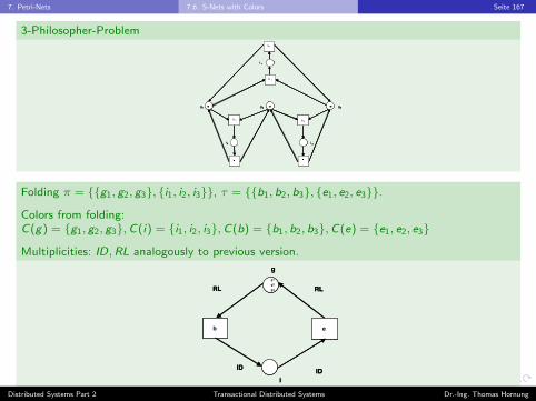
7. Petri-Nets 7.6. S-Nets with Colors Seite 167
3-Philosopher-Problem
i 1
b 2
e2
e3
b 3
b 1
e1
i 2 i 3
g 1 g 2 g 3
i 1
b 2
e2
e3
b 3
b 1
e1
i 2 i 3
g 1 g 2 g 3
i 1
b 2
e2
e3
b 3
b 1
e1
i 2 i 3
g 1 g 2 g 3
Folding π = {{g1, g2, g3}, {i1, i2, i3}}, τ = {{b1, b2, b3}, {e1, e2, e3}}.
Colors from folding:C(g) = {g1, g2, g3},C(i) = {i1, i2, i3},C(b) = {b1, b2, b3},C(e) = {e1, e2, e3}
Multiplicities: ID,RL analogously to previous version.
b e
ID
g
RL
g1
g2
g3 RL
IDi
b e
ID
g
RL
g1
g2
g3 RL
IDi
Distributed Systems Part 2 Transactional Distributed Systems Dr.-Ing. Thomas Hornung
7. Petri-Nets 7.6. S-Nets with Colors Seite 168
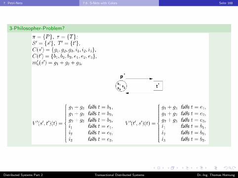
3-Philosopher-Problem?
Distributed Systems Part 2 Transactional Distributed Systems Dr.-Ing. Thomas Hornung

7. Petri-Nets 7.6. S-Nets with Colors Seite 169
Given π = {q1, . . . , qk}, τ = {u1, . . . , un}.
The folding GN(π, τ) := (P ′,T ′,F ′,C ′,V ′,m′0) of N is defined as follows:
P′ := {p′1, . . . , p′k}; T′ := {t′1, . . . , t′n},
C ′(p′i ) = qi fur i = 1, . . . , k; C ′(t′j ) = uj fur j = 1, . . . , n,
F ′ := {(p′, t′) | C ′(p′)× C ′(t′) ∩ F 6= ∅} ∪{(t′, p′) | C ′(t′)× C ′(p′) ∩ F 6= ∅},
f ′ = (p′, t′) ∈ F ′: V ′(f ′) is defined (t ∈ C ′(t′)):
V ′(f ′)(t) =∑
p∈C ′(p′)t−(p) · p,
f ′ = (t′, p′) ∈ F ′: V ′(f ′) is defined (t ∈ C ′(t′)):
V ′(f ′)(t) =∑
p∈C ′(p′)t+(p) · p,
m′0(p′) :=∑
p∈C ′(p′)m0(p) · p.
Distributed Systems Part 2 Transactional Distributed Systems Dr.-Ing. Thomas Hornung

7. Petri-Nets 7.6. S-Nets with Colors Seite 170
Given π = {q1, . . . , qk}, τ = {u1, . . . , un}.
The folding GN(π, τ) := (P ′,T ′,F ′,C ′,V ′,m′0) of N is defined as follows:
P′ := {p′1, . . . , p′k}; T′ := {t′1, . . . , t′n},
C ′(p′i ) = qi fur i = 1, . . . , k; C ′(t′j ) = uj fur j = 1, . . . , n,
F ′ := {(p′, t′) | C ′(p′)× C ′(t′) ∩ F 6= ∅} ∪{(t′, p′) | C ′(t′)× C ′(p′) ∩ F 6= ∅},
f ′ = (p′, t′) ∈ F ′: V ′(f ′) is defined (t ∈ C ′(t′)):
V ′(f ′)(t) =∑
p∈C ′(p′)t−(p) · p,
f ′ = (t′, p′) ∈ F ′: V ′(f ′) is defined (t ∈ C ′(t′)):
V ′(f ′)(t) =∑
p∈C ′(p′)t+(p) · p,
m′0(p′) :=∑
p∈C ′(p′)m0(p) · p.
Distributed Systems Part 2 Transactional Distributed Systems Dr.-Ing. Thomas Hornung

7. Petri-Nets 7.6. S-Nets with Colors Seite 171
Given π = {q1, . . . , qk}, τ = {u1, . . . , un}.
The folding GN(π, τ) := (P ′,T ′,F ′,C ′,V ′,m′0) of N is defined as follows:
P′ := {p′1, . . . , p′k}; T′ := {t′1, . . . , t′n},
C ′(p′i ) = qi fur i = 1, . . . , k; C ′(t′j ) = uj fur j = 1, . . . , n,
F ′ := {(p′, t′) | C ′(p′)× C ′(t′) ∩ F 6= ∅} ∪{(t′, p′) | C ′(t′)× C ′(p′) ∩ F 6= ∅},
f ′ = (p′, t′) ∈ F ′: V ′(f ′) is defined (t ∈ C ′(t′)):
V ′(f ′)(t) =∑
p∈C ′(p′)t−(p) · p,
f ′ = (t′, p′) ∈ F ′: V ′(f ′) is defined (t ∈ C ′(t′)):
V ′(f ′)(t) =∑
p∈C ′(p′)t+(p) · p,
m′0(p′) :=∑
p∈C ′(p′)m0(p) · p.
Distributed Systems Part 2 Transactional Distributed Systems Dr.-Ing. Thomas Hornung

7. Petri-Nets 7.6. S-Nets with Colors Seite 172
Given π = {q1, . . . , qk}, τ = {u1, . . . , un}.
The folding GN(π, τ) := (P ′,T ′,F ′,C ′,V ′,m′0) of N is defined as follows:
P′ := {p′1, . . . , p′k}; T′ := {t′1, . . . , t′n},
C ′(p′i ) = qi fur i = 1, . . . , k; C ′(t′j ) = uj fur j = 1, . . . , n,
F ′ := {(p′, t′) | C ′(p′)× C ′(t′) ∩ F 6= ∅} ∪{(t′, p′) | C ′(t′)× C ′(p′) ∩ F 6= ∅},
f ′ = (p′, t′) ∈ F ′: V ′(f ′) is defined (t ∈ C ′(t′)):
V ′(f ′)(t) =∑
p∈C ′(p′)t−(p) · p,
f ′ = (t′, p′) ∈ F ′: V ′(f ′) is defined (t ∈ C ′(t′)):
V ′(f ′)(t) =∑
p∈C ′(p′)t+(p) · p,
m′0(p′) :=∑
p∈C ′(p′)m0(p) · p.
Distributed Systems Part 2 Transactional Distributed Systems Dr.-Ing. Thomas Hornung

7. Petri-Nets 7.6. S-Nets with Colors Seite 173
Given π = {q1, . . . , qk}, τ = {u1, . . . , un}.
The folding GN(π, τ) := (P ′,T ′,F ′,C ′,V ′,m′0) of N is defined as follows:
P′ := {p′1, . . . , p′k}; T′ := {t′1, . . . , t′n},
C ′(p′i ) = qi fur i = 1, . . . , k; C ′(t′j ) = uj fur j = 1, . . . , n,
F ′ := {(p′, t′) | C ′(p′)× C ′(t′) ∩ F 6= ∅} ∪{(t′, p′) | C ′(t′)× C ′(p′) ∩ F 6= ∅},
f ′ = (p′, t′) ∈ F ′: V ′(f ′) is defined (t ∈ C ′(t′)):
V ′(f ′)(t) =∑
p∈C ′(p′)t−(p) · p,
f ′ = (t′, p′) ∈ F ′: V ′(f ′) is defined (t ∈ C ′(t′)):
V ′(f ′)(t) =∑
p∈C ′(p′)t+(p) · p,
m′0(p′) :=∑
p∈C ′(p′)m0(p) · p.
Distributed Systems Part 2 Transactional Distributed Systems Dr.-Ing. Thomas Hornung
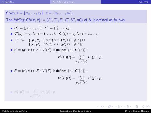
7. Petri-Nets 7.6. S-Nets with Colors Seite 174
Given π = {q1, . . . , qk}, τ = {u1, . . . , un}.
The folding GN(π, τ) := (P ′,T ′,F ′,C ′,V ′,m′0) of N is defined as follows:
P′ := {p′1, . . . , p′k}; T′ := {t′1, . . . , t′n},
C ′(p′i ) = qi fur i = 1, . . . , k; C ′(t′j ) = uj fur j = 1, . . . , n,
F ′ := {(p′, t′) | C ′(p′)× C ′(t′) ∩ F 6= ∅} ∪{(t′, p′) | C ′(t′)× C ′(p′) ∩ F 6= ∅},
f ′ = (p′, t′) ∈ F ′: V ′(f ′) is defined (t ∈ C ′(t′)):
V ′(f ′)(t) =∑
p∈C ′(p′)t−(p) · p,
f ′ = (t′, p′) ∈ F ′: V ′(f ′) is defined (t ∈ C ′(t′)):
V ′(f ′)(t) =∑
p∈C ′(p′)t+(p) · p,
m′0(p′) :=∑
p∈C ′(p′)m0(p) · p.
Distributed Systems Part 2 Transactional Distributed Systems Dr.-Ing. Thomas Hornung

7. Petri-Nets 7.6. S-Nets with Colors Seite 175
Given π = {q1, . . . , qk}, τ = {u1, . . . , un}.
The folding GN(π, τ) := (P ′,T ′,F ′,C ′,V ′,m′0) of N is defined as follows:
P′ := {p′1, . . . , p′k}; T′ := {t′1, . . . , t′n},
C ′(p′i ) = qi fur i = 1, . . . , k; C ′(t′j ) = uj fur j = 1, . . . , n,
F ′ := {(p′, t′) | C ′(p′)× C ′(t′) ∩ F 6= ∅} ∪{(t′, p′) | C ′(t′)× C ′(p′) ∩ F 6= ∅},
f ′ = (p′, t′) ∈ F ′: V ′(f ′) is defined (t ∈ C ′(t′)):
V ′(f ′)(t) =∑
p∈C ′(p′)t−(p) · p,
f ′ = (t′, p′) ∈ F ′: V ′(f ′) is defined (t ∈ C ′(t′)):
V ′(f ′)(t) =∑
p∈C ′(p′)t+(p) · p,
m′0(p′) :=∑
p∈C ′(p′)m0(p) · p.
Distributed Systems Part 2 Transactional Distributed Systems Dr.-Ing. Thomas Hornung

7. Petri-Nets 7.6. S-Nets with Colors Seite 176
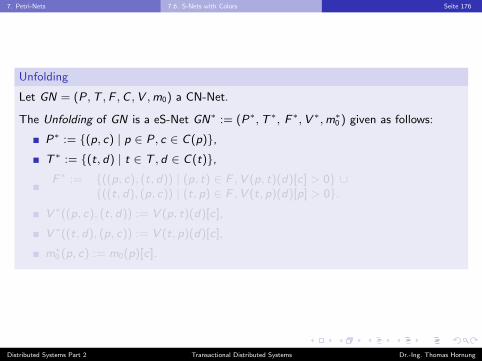
Unfolding
Let GN = (P,T ,F ,C ,V ,m0) a CN-Net.
The Unfolding of GN is a eS-Net GN∗ := (P∗,T ∗, F ∗,V ∗,m∗0 ) given as follows:
P∗ := {(p, c) | p ∈ P, c ∈ C(p)},T ∗ := {(t, d) | t ∈ T , d ∈ C(t)},F ∗ := {((p, c), (t, d)) | (p, t) ∈ F ,V (p, t)(d)[c] > 0} ∪
{((t, d), (p, c)) | (t, p) ∈ F ,V (t, p)(d)[p] > 0}.V ∗((p, c), (t, d)) := V (p, t)(d)[c],
V ∗((t, d), (p, c)) := V (t, p)(d)[c],
m∗0 (p, c) := m0(p)[c].
Distributed Systems Part 2 Transactional Distributed Systems Dr.-Ing. Thomas Hornung

7. Petri-Nets 7.6. S-Nets with Colors Seite 177
Unfolding
Let GN = (P,T ,F ,C ,V ,m0) a CN-Net.
The Unfolding of GN is a eS-Net GN∗ := (P∗,T ∗, F ∗,V ∗,m∗0 ) given as follows:
P∗ := {(p, c) | p ∈ P, c ∈ C(p)},T ∗ := {(t, d) | t ∈ T , d ∈ C(t)},F ∗ := {((p, c), (t, d)) | (p, t) ∈ F ,V (p, t)(d)[c] > 0} ∪
{((t, d), (p, c)) | (t, p) ∈ F ,V (t, p)(d)[p] > 0}.V ∗((p, c), (t, d)) := V (p, t)(d)[c],
V ∗((t, d), (p, c)) := V (t, p)(d)[c],
m∗0 (p, c) := m0(p)[c].
Distributed Systems Part 2 Transactional Distributed Systems Dr.-Ing. Thomas Hornung

7. Petri-Nets 7.6. S-Nets with Colors Seite 178
Unfolding
Let GN = (P,T ,F ,C ,V ,m0) a CN-Net.
The Unfolding of GN is a eS-Net GN∗ := (P∗,T ∗, F ∗,V ∗,m∗0 ) given as follows:
P∗ := {(p, c) | p ∈ P, c ∈ C(p)},T ∗ := {(t, d) | t ∈ T , d ∈ C(t)},F ∗ := {((p, c), (t, d)) | (p, t) ∈ F ,V (p, t)(d)[c] > 0} ∪
{((t, d), (p, c)) | (t, p) ∈ F ,V (t, p)(d)[p] > 0}.V ∗((p, c), (t, d)) := V (p, t)(d)[c],
V ∗((t, d), (p, c)) := V (t, p)(d)[c],
m∗0 (p, c) := m0(p)[c].
Distributed Systems Part 2 Transactional Distributed Systems Dr.-Ing. Thomas Hornung

7. Petri-Nets 7.6. S-Nets with Colors Seite 179
Unfolding
Let GN = (P,T ,F ,C ,V ,m0) a CN-Net.
The Unfolding of GN is a eS-Net GN∗ := (P∗,T ∗, F ∗,V ∗,m∗0 ) given as follows:
P∗ := {(p, c) | p ∈ P, c ∈ C(p)},T ∗ := {(t, d) | t ∈ T , d ∈ C(t)},F ∗ := {((p, c), (t, d)) | (p, t) ∈ F ,V (p, t)(d)[c] > 0} ∪
{((t, d), (p, c)) | (t, p) ∈ F ,V (t, p)(d)[p] > 0}.V ∗((p, c), (t, d)) := V (p, t)(d)[c],
V ∗((t, d), (p, c)) := V (t, p)(d)[c],
m∗0 (p, c) := m0(p)[c].
Distributed Systems Part 2 Transactional Distributed Systems Dr.-Ing. Thomas Hornung

7. Petri-Nets 7.6. S-Nets with Colors Seite 180
Definition
Let E be a certain property of a net, e.g. boundedness, liveness, or reachability.
A CS-Net GN has property E , whenever its unfolding GN∗ has property E .
Analysis of colored System Nets
Analyse unfolding:
Advantage: Methods exist,Pitfall: Unfoldings may be huge eS-Nets.
Analyse colored net:
Reachability graph and coverability graph can be defined in analogous wayto eS-Nets.There exists a theory for invariants, as well.Tools for simulation and analysis are available.
Distributed Systems Part 2 Transactional Distributed Systems Dr.-Ing. Thomas Hornung
7. Petri-Nets 7.6. S-Nets with Colors Seite 181
Definition
Let E be a certain property of a net, e.g. boundedness, liveness, or reachability.
A CS-Net GN has property E , whenever its unfolding GN∗ has property E .
Analysis of colored System Nets
Analyse unfolding:
Advantage: Methods exist,Pitfall: Unfoldings may be huge eS-Nets.
Analyse colored net:
Reachability graph and coverability graph can be defined in analogous wayto eS-Nets.There exists a theory for invariants, as well.Tools for simulation and analysis are available.
Distributed Systems Part 2 Transactional Distributed Systems Dr.-Ing. Thomas Hornung

7. Petri-Nets 7.6. S-Nets with Colors Seite 182
Definition
Let E be a certain property of a net, e.g. boundedness, liveness, or reachability.
A CS-Net GN has property E , whenever its unfolding GN∗ has property E .
Analysis of colored System Nets
Analyse unfolding:
Advantage: Methods exist,Pitfall: Unfoldings may be huge eS-Nets.
Analyse colored net:
Reachability graph and coverability graph can be defined in analogous wayto eS-Nets.There exists a theory for invariants, as well.Tools for simulation and analysis are available.
Distributed Systems Part 2 Transactional Distributed Systems Dr.-Ing. Thomas Hornung
7. Petri-Nets 7.6. S-Nets with Colors Seite 183
Definition
Let E be a certain property of a net, e.g. boundedness, liveness, or reachability.
A CS-Net GN has property E , whenever its unfolding GN∗ has property E .
Analysis of colored System Nets
Analyse unfolding:
Advantage: Methods exist,Pitfall: Unfoldings may be huge eS-Nets.
Analyse colored net:
Reachability graph and coverability graph can be defined in analogous wayto eS-Nets.There exists a theory for invariants, as well.Tools for simulation and analysis are available.
Distributed Systems Part 2 Transactional Distributed Systems Dr.-Ing. Thomas Hornung