mutually and laterally constrained inversion of cves and ... · tem data: a case study anders v....

© 2007 European Association of Geoscientists & Engineers 115

Mutually and laterally constrained inversion of CVES and TEM data: a case study

Anders V. Christiansen*, Esben Auken, Nikolai Foged and Kurt I. Sørensen

The Hydrogeophysics Group, University of Aarhus, Department of Earth Sciences, Finlandsgade 8, Denmark

Received February 2005, revision accepted June 2006

ABSTRACTMutually constrained inversion in combination with laterally constrained inversion (MCI-LCI) between transient electromagnetic (TEM) and direct current (DC) resistivity methods was success-fully used to characterize a buried valley structure. Although both methods measure, in some sense, the electrical resistivity, or conductivity, of the subsurface, they sample different volumes and have different sensitivities, which are exploited with mutually and laterally constrained inversion of combined, coincident profile data sets. The output models incorporate the information from both data sets to obtain optimum layered 1D models, fitting both data sets and constraints. The set-up of constraints contains three parts. First, we constrain the individual data sets along their profile using lateral constraints producing a chain of TEM data and a chain of DC data. Next, we merge the information from these two chains by setting up mutual constraints between the TEM and the DC models. Finally, we adjust the mutual constraints to resemble the increasing sampling volumes with depth, i.e. wide constraints at large depths and short constraints at shallow depths. All data sets are inverted simultaneously; a common objective function is minimized, and the number of output models is equal to the number of 1D soundings. The lateral and mutual constraints are part of the inversion, and consequently the output models are balanced between the constraints and the data-model fit. Information from one model will spread to the neighbour-ing models through the constraints, helping to resolve parameters that are poorly resolved by any of the individual data sets. A field example illustrates that MCI-LCI allows the governing information from each method to dominate the inversion process. Thus, the model resolution in both the shallow and the deeper parts of the model is significantly enhanced. This could not be obtained by inverting the two data sets separately with a subsequent comparison of the output models. Our results are confirmed by drill-hole data.

are data sets while constraining the models with lateral and mutual constraints. This allows for coincident models to differ, reflecting their different sensitivities to the subsurface parame-ters. We combine time-domain electromagnetic (TEM) and continuous vertical electrical sounding (CVES) data.

THE TEM AND GEOELECTRIC METHODSThe TEM method is an electromagnetic induction technique in which the response of the earth to an electromagnetic impulse is measured in the time domain. A thorough discussion of the TEM method and the interpretation of TEM data can be found in Nabighian and Macnae (1991). As with all electromagnetic dif-fusion methods, the TEM method has a decreasing resolution capability with depth, and high-resistivity layers are poorly resolved. Sequences of thin layers are combined into an effective single layer with an average bulk resistivity. Near-surface layers will also be recovered as one layer with an average resistivity,

INTRODUCTIONThe amount of data collected in geoelectric as well as in electro-magnetic (EM) surveys has increased substantially with the introduction of various continuous mapping systems. In the case of collocated profile data, a common interpretation involving all data sets is often sought. However, this can be problematic because different geophysical methods are sensitive to different physical properties within the earth. Over the years, a number of different approaches to joint or combined inversion of different data sets have been presented by, for example, Vozoff and Jupp (1975), Raiche et al. (1985), Lines et al. (1988), Meju (1996), Haber and Oldenburg (1997) and Wisén and Christiansen (2005). These approaches often aimed at producing one model for two distinct data sets. In the approach presented here, we produce the same number of models as there

* [email protected]

Near Surface Geophysics, 2007, 115-123

A.V. Christiansen et al.116

© 2007 European Association of Geoscientists & Engineers, Near Surface Geophysics, 2007, 5, 115-123115-123

because little information is present at very early times. The cur-rent flow in the ground induced by a TEM system is horizontal (for a 1D earth) meaning that anisotropy is not an issue. The TEM data presented here was acquired with the HiTEM system with a penetration depth of approximately 250 m (Danielsen et al. 2003; Sørensen et al. 2005). With the DC resistivity, or the continuous vertical electrical sounding (CVES) method (Dahlin 2001), a current is injected into the earth and the resulting voltage is a response of the resis-tivity of the subsurface. DC resistivity measurements have the highest resolution capabilities closest to the surface, decreasing downwards. Near-surface inhomogeneities can cause static shifts in the data (Meju 2005). The current patterns from the DC method cross through layers, which means that DC data are inherently influenced by anisotropy (Christensen 2000). Anisotropy causes layer thicknesses to be overestimated. For the TEM method, the early time data are heavily influ-enced by the current turn-off ramp and the low-pass filters in the receiver and the receiver coil. As a consequence, the ramp and the filters must be included in the forward-modelling algorithm

(Fitterman and Anderson 1987; Effersø et al. 1999) in order to avoid a systematic bias of the resistivities of the near-surface layers. Such a bias introduces artificial thin high- or low-resistiv-ity layers when performing the combined inversion of the TEM and the CVES data. We employed a continuous gradient array (Dahlin and Zhou 2006) with 3555 data points acquired along a 1 km profile sam-pled with a 5 m electrode spacing. The penetration depth for this set-up is 50–80 m, depending on the geology.

JOINT INVERSION AND INTERPRETATIONOver the years, various schemes have been introduced to invert two distinct data sets, and various terminologies have been used to describe these methods. Separate inversion of two related but individual data sets produces two individual models that might, or might not, be correlated. Joint inversion, a rather generic name, implies that two related data sets are used in the same objective function, and one model is produced through the opti-mization process (Vozoff and Jupp 1975). Haber and Oldenburg (1997) introduced a generalized con-cept of combining dissimilar data sets. They assume that the models underlying the data sets have a common structure, and the joint objective function is posed to minimize the difference in structure between the two models. The concept of combining different data types sharing resistivity as the common physical parameter has been presented by Raiche et al. (1985), Meju (1996), Santos et al. (1997) and Albouy et al. (2001).

LATERALLY AND MUTUALLY CONSTRAINED INVERSIONWe use the term laterally constrained inversion (LCI) for invert-ing data along a profile through minimizing a common objective function (Auken et al. 2005). The LCI is a parametrized inver-sion of data of the same type with lateral constraints on the model parameters between neighbouring models. The lateral constraints can be considered as a priori information on the geological variability within the area where the measurements are taken. The resulting model section is laterally smooth with sharp layer interfaces as depicted in Fig. 1. The LCI offers a sensitivity analysis of the model parameters, which is essential for evaluating the integrity of the model. Furthermore, it is pos-

FIGURE 1

The LCI model is a section of stitched-together 1D models combined with lateral constraints.

FIGURE 2

The MCI model concept where the different data types are connected via

constraints on the model parameters.

Mutually and laterally constrained inversion 117


sible to add a priori information by constraining model param-eters, such as a depth-to-layer interface based on lithology from drill-hole data. Mutually constrained inversion (MCI) is a procedure where two or more coincident but different data sets, such as TEM and DC resistivity data, are inverted to produce the same number of models with a correlation between the models established through equality constraints between corresponding parameters. This is outlined in Fig. 2. In contrast to the joint inversion approach, in which a common object function is minimized resulting in one inverse model, MCI results in the same number of models as data sets. Thus, the MCI scheme offers a continuum with the individual inversions and the joint inversions as end-member cases. Hence, a static shift parameter or coefficient of anisotropy is not explicitly required for a convergent solution as in a joint inversion (Christensen 2000; Auken et al. 2001). Here we combine the LCI and the MCI concepts and apply the result to the TEM and CVES profile data. The TEM and CVES data sets are internally connected with lateral constraints to form a chain along the profile. The TEM LCI chain is then connected to the CVES LCI chain through mutual constraints from individual TEM soundings to CVES soundings. The LCI produces a laterally smooth model with sharp layer boundaries. The MCI allows for information to migrate between the TEM data and CVES data and also allows for dissimilar models when CVES and TEM data sets are coincident.

METHODOLOGYInversionThe laterally constrained inversion scheme is described in detail by Auken et al. (2005) and for combined inversion of DC resis-tivity and surface-wave seismic data by Wisén and Christiansen (2005). The model is a section of stitched-together 1D models along a profile. The lateral distance between the models is determined

by the sampling density of the data and may be non-equidistant. The parameters are layer resistivities and thicknesses. The CVES data are divided into soundings where all those with a lateral focus point in a specific section combine into a data set (a sounding) referring to a single 1D model, as illustrated in Fig. 3. The lateral focus points of the gradient array configura-tions are found by numerical integration of the 2D sensitivity distributions. The HiTEM system combines a central-loop low-moment sounding with an offset-loop high-moment sounding. The receiver is offset 70 m in the high-moment sounding. Hence, pairs of two distinct soundings, separated by 70 m corresponding to the offset distance, are assembled to create a full data set (Danielsen et al. 2003). All data sets are inverted simultaneously, minimizing a common objective function including the lateral constraints and the mutual constraints. Consequently, the output models form a balance between the constraints, the physics of the two methods and the data. Model parameters with little influence on the data will be controlled by the constraints and vice versa. Due to the lateral con-straints, information from one model will spread to neighbouring models. The mutual constraints ensure that information flows from the DC resistivity models to the TEM models and vice versa.

ConstraintsTo set up the lateral and mutual constraints, we have to consider the unequal sampling density and the different sensitivity of the two methods. For each 1D sounding, we have a 1D model as sketched in Fig. 4. The constraints between the models are based on the following three points: 1 Lateral constraints. Every DC resistivity model is constrained

to its nearest DC resistivity models in both directions. Similarly, every TEM model is constrained to its neighbour-ing models on each side. This is illustrated in Fig. 4(b).

2 Mutual constraints. The TEM and the DC resistivity models

FIGURE 3

The CVES profile is divided into N data sets. The dots represent the focus point of a 4-pole array. The vertical dashed lines depict 1D soundings.



are constrained to each other within a distance that reflects the footprint of the TEM method, as illustrated in Fig. 4(c). We have chosen to use the depth of the layer as a reference for the width of the constraint, so that the deeper the layer the wider the constraint between the TEM and the DC resistivity mod-els.

3 All lateral constraints Cl are scaled according to the model separation d, using a empirical power-law formulation,

(1)

where Cr is a reference constraint, which is a function of some reference distance dr. Therefore, if the distance between two constrained models is twice that of the reference distance, the constraint values between the two models are multiplied by a factor of 2p. In this survey, p was set at 0.5 by trial-and-error, achieving a subsurface image with sufficient complexity while maintaining laterally coherent layers. Combining the constraints applied in the above points 1 and 2 yields the full set of constraints as sketched in Fig. 4(d). The lateral and mutual constraints can be applied on thick-nesses or depths. Constraints on depths favour horizontal layer boundaries whereas constraints on thicknesses favour constant thickness in layers. The following example illustrates the differ-ence: imagine a case where the thickness of layer 1 increases

FIGURE 4

Constraint settings. (a) A simplified sketch of the distribution of TEM

and geoelectric DC soundings and their corresponding models. The two

profile lines have been separated for clarity. (b) Lateral constraints

between the geoelectric and the TEM data are applied. (c) Mutual con-

straints between the geoelectric and TEM data are applied. (d) A sum-

mary of the total set of constraints.

FIGURE 5

(a) The survey area located on the

Jutland peninsula, Denmark. (b)

Details of the field area, where

black dots are centre locations of

HiTEM soundings, the black

lines are the CVES profiles and

the red star is a deep drill-hole.

The underlying contour map is

the elevation of the Tertiary clay

(the good conductor), constructed

from roughly 200 existing TEM

soundings in the survey area.



from 1m to 10 m over the profile, while all other thicknesses are unchanged. In the case of constraints on thicknesses, only layer 1 is penalized even though all layer boundaries change position. If, instead, constraints on depths are applied, all boundaries are penalized for the change in thickness of layer 1. We have used lateral constraints on depths for this case. Constraints are relative for resistivities and absolute for depths. We used reference constraints Cr of 1.1 (approximately 10%) on resistivities and 5 m on depths. The reference distance dr is 10 m, reflecting the sounding distance employed for the CVES data. This means that models are allowed to vary by approximately 10% in resistivities and ±5 m on layer depths over 10 m. To allow for rapid variations of the near-surface resistivity for the CVES models, a thin top-layer is added with no constraints. The depth-dependent mutual constraints from the TEM models to the CVES models are based on two considerations. Firstly, lat-erally wide constraints on the TEM to CVES data in the deeper parts of the section emphasize structures defined by the TEM while still fitting the CVES data; secondly, the narrow TEM to CVES constraints in the upper section allow the CVES models to vary rapidly while not conflicting with the TEM data.

Analysis of model estimation uncertaintyThe laterally and mutually constrained inversion is an overdeter-mined problem. Therefore, we can produce a sensitivity analysis of the model parameters, which is essential to assess the resolu-tion of the inverted model (Tarantola and Valette 1982). Because the model parameters are represented as logarithms, the analysis gives a standard deviation factor (STDF) for the parameter. Thus, the theoretical case of perfect resolution has STDF=1; STDF=1.1 is approximately equivalent to an error of 10%. Well-resolved parameters have STDF<1.2, moderately resolved parameters fall within the range 1.2<STDF<1.5, poorly resolved parameters are in the range 1.5<STDF<2, and unre-solved parameters have STDF>2.

The Tinning field studyThe objective of the Tinning field study was to characterize a buried-valley system incised in Tertiary clay. The Tinning field area is of great interest to the 270 000 inhabitants of the city of Aarhus, due to its status as possible groundwater recharge area. In Denmark, buried valleys are found to be between 0.5 and 4 km wide and up to 350 m deep (Jørgensen et al. 2003). The geome-try of the buried valleys as well as the resistivity distribution is important for ascertaining whether the valley systems are poten-tial groundwater reservoirs. The location of the survey area is shown on the map in Fig. 5(a). The field area lies on a flat glacial outwash plain, which means that it is impossible to predict the presence of a buried valley from the surface topography. However, an initial TEM field campaign clearly depicted the presence of the buried valley, as shown in Fig. 5(b). This result led to the detailed mapping presented here.

FIGURE 6

(a) Data containing both segments of the HiTEM sounding; (b) the cor-

responding 1D model from a sounding at coordinate 921 m (see Fig. 7

for location). The low-moment data are marked with the black error bars;

the high-moment data with grey error bars. The model responses from

the two resulting models in (b) are shown by solid lines.



The Tertiary clay present in the entire area is covered by various glacial deposits, which are the prime target for new water-extraction drill-holes. We acquired both HiTEM and CVES data in the survey area on profile lines approximately perpendicular to the strike of the incised valley. The positioning of the HiTEM soundings, the CVES profiles and a deep drill-hole are illustrated on the map in Fig. 5(b). In order to evaluate the results of the combined inversion of TEM and CVES data, we start by presenting normal LCI profiles using the TEM and CVES data separately. This shows what can be achieved if the methods are applied independently.

Results of LCI of TEM dataThe high-moment and the low-moment segments of the HiTEM soundings were treated as individual soundings. A representative plot of a full HiTEM sounding with both segments and the resulting model is shown in Fig. 6. An LCI model of profile 1 constructed from HiTEM soundings is shown in Fig. 7. The model section in Fig. 7(a) reveals a valley structure incised in the bottom low-resistivity (<10 Ωm) layer. At the cen-tre of the profile, the depth to the bottom of the valley is approx-imately 120 m. The low-resistivity layer is actually composed of two layers with slightly different resistivities. A near-surface layer, 40 m thick and with resistivity approximately 30–40 Ωm, overlies a high-resistivity layer. This overall layering is con-firmed by drill-hole log data at coordinate 800 m, but variations within the top layer, as identified by the drill-hole data, collapse into one layer in the HiTEM 1D LCI model due to the limited resolution at shallow depths. Also the resistivities of the top high-resistivity layers are overestimated by the TEM data. The data residuals, shown in Fig. 7(b), are all well below 1, implying that the data fit within the data error. The panels in Fig. 7(c) show model resolution for each parameter (as noted to the left) in each 1D model. The parameter analyses reveal

mostly well-determined parameters, with the resistivity of the second layer being the exception. The high resistivity of this layer is poorly determined as is to be expected with the TEM method.

Results of LCI of CVES dataThe results from the CVES data alone are shown in Fig. 8. The data are presented in Fig. 8(a) in pseudosection format. Note that between coordinates 1000 and 1150 m, several data points were omitted due to noise. The result of a smooth minimum-structure inversion is shown in Fig. 8(b), along with the resistivity results from the drill-hole. The general structure is a near-surface layer of resistivity 20–50 Ωm, with some high-resistivity contributions at the surface, overlying a high-resistivity layer. At the ends, a low-resistivity layer is identified at the bottom. The geometry of the buried val-ley is poorly defined and an exact thickness of the high-resistiv-ity layer is impossible to estimate. The resistivity of the thick high-resistivity layer is overestimated compared to the electrical log, but the depth to the top of the layer in the centre of the pro-file is well defined and corresponds well with the log. The data residuals for the minimum-structure inversion in Fig. 8(c) reveal that data are mainly well fitted with residuals below 1. Figure 8(d) shows the result of the LCI of the CVES data. The model contains five layers, but the thin top layer is barely visible in this presentation. As was the case with the smooth inversion, a high-resistivity layer (~300–600 Ωm) and a conductive base-ment (<10 Ωm) indicate a buried valley incised in the Tertiary clay, overlain by a layer of resistivity 20–50 Ωm. The high resis-tivity of the valley layer is still overestimated compared to the electrical log, but the upper boundary is sharp and well defined. In the LCI model, the conductive basement is evident in the entire section due to the constraints, even though it is barely vis-ible in the data in the centre of the profile, as seen in the selected

FIGURE 7

(a) LCI section constructed from

HiTEM soundings. Drill-hole

resistivity logging data are pre-

sented with the same colour scale

as the LCI section. (b) Data resid-

uals of the TEM soundings and

(c) parameter analyses. The anal-

ysis uses a four-colour code rang-

ing from red (well-determined) to

blue (undetermined).



sounding in Fig. 9(a). The resulting model is shown in Fig. 9(b). The sounding is located at coordinate 920 m. At shallow depths, a thin high-resistivity layer is found at 5–8 m depth corresponding to a sandy unit described in the drill-hole log; this is not visible on the resistivity log as no data are present in the upper 10 m. The data residuals in Fig. 8(e) reveal misfits generally around 1, or below. Exceptions are the soundings from 970 m to 1300 m that have data residuals between 1 and 3. The analyses in Fig. 8(e) reveal well-determined parameters especially concerning the parameters of the third and fourth layers. The third layer is the low-resistivity layer in the top of the model which overlies the fourth layer, defining the high-resistivity valley structure.

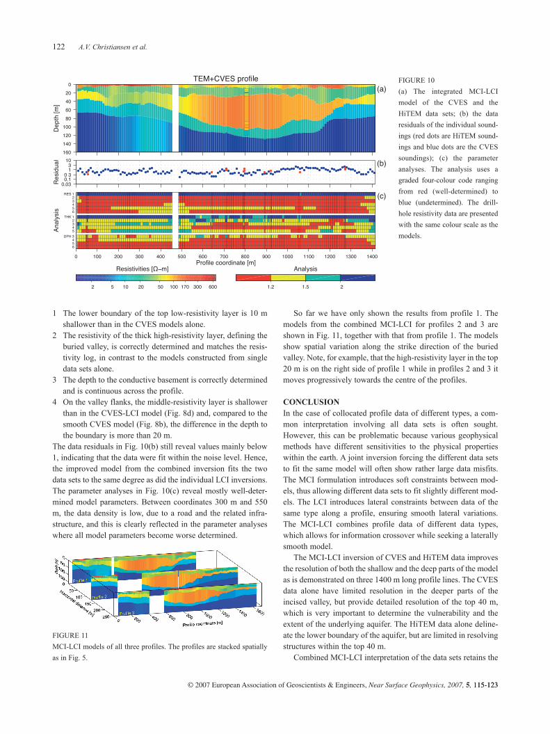
Results of the combined MCI-LCI of TEM and CVES dataThe drilling data, as well as the integrated LCI inversion of the full HiTEM and the CVES data, are presented in Fig. 10(a). The model has six layers, including a barely visible top layer. Comparison of the integrated LCI model with the TEM model of Fig. 7 and the CVES models in Fig. 8 reveals details that could not have been extracted from the individual inversion models alone. The four most prominent elements are:

FIGURE 8

Results for the data from the

CVES profile: (a) pseudosection

format; (b) a smooth minimum-

structure inversion model; (c) the

data residuals for the smooth

minimum-structure inversion in

(b); (d) a 1D-LCI inversion

model; (e) data residuals of the

individual soundings; (f) the

parameter analyses. The analysis

uses a graded four-colour code

ranging from red (well-deter-

mined) to blue (undetermined).

The drill-hole resistivities are

presented using the same colour

scale as the models.

FIGURE 9

(a) CVES sounding data plotted as a function of the focus depth; (b) the

corresponding 1D model from the sounding at coordinate 920 m. The data

are plotted with error bars, and the 1D model is drawn as a solid line.



1 The lower boundary of the top low-resistivity layer is 10 m shallower than in the CVES models alone.

2 The resistivity of the thick high-resistivity layer, defining the buried valley, is correctly determined and matches the resis-tivity log, in contrast to the models constructed from single data sets alone.

3 The depth to the conductive basement is correctly determined and is continuous across the profile.

4 On the valley flanks, the middle-resistivity layer is shallower than in the CVES-LCI model (Fig. 8d) and, compared to the smooth CVES model (Fig. 8b), the difference in the depth to the boundary is more than 20 m.

The data residuals in Fig. 10(b) still reveal values mainly below 1, indicating that the data were fit within the noise level. Hence, the improved model from the combined inversion fits the two data sets to the same degree as did the individual LCI inversions. The parameter analyses in Fig. 10(c) reveal mostly well-deter-mined model parameters. Between coordinates 300 m and 550 m, the data density is low, due to a road and the related infra-structure, and this is clearly reflected in the parameter analyses where all model parameters become worse determined.

So far we have only shown the results from profile 1. The models from the combined MCI-LCI for profiles 2 and 3 are shown in Fig. 11, together with that from profile 1. The models show spatial variation along the strike direction of the buried valley. Note, for example, that the high-resistivity layer in the top 20 m is on the right side of profile 1 while in profiles 2 and 3 it moves progressively towards the centre of the profiles.

CONCLUSIONIn the case of collocated profile data of different types, a com-mon interpretation involving all data sets is often sought. However, this can be problematic because various geophysical methods have different sensitivities to the physical properties within the earth. A joint inversion forcing the different data sets to fit the same model will often show rather large data misfits. The MCI formulation introduces soft constraints between mod-els, thus allowing different data sets to fit slightly different mod-els. The LCI introduces lateral constraints between data of the same type along a profile, ensuring smooth lateral variations. The MCI-LCI combines profile data of different data types, which allows for information crossover while seeking a laterally smooth model. The MCI-LCI inversion of CVES and HiTEM data improves the resolution of both the shallow and the deep parts of the model as is demonstrated on three 1400 m long profile lines. The CVES data alone have limited resolution in the deeper parts of the incised valley, but provide detailed resolution of the top 40 m, which is very important to determine the vulnerability and the extent of the underlying aquifer. The HiTEM data alone deline-ate the lower boundary of the aquifer, but are limited in resolving structures within the top 40 m. Combined MCI-LCI interpretation of the data sets retains the

FIGURE 10

(a) The integrated MCI-LCI

model of the CVES and the

HiTEM data sets; (b) the data

residuals of the individual sound-

ings (red dots are HiTEM sound-

ings and blue dots are the CVES

soundings); (c) the parameter

analyses. The analysis uses a

graded four-colour code ranging

from red (well-determined) to

blue (undetermined). The drill-

hole resistivity data are presented

with the same colour scale as the

models.

FIGURE 11

MCI-LCI models of all three profiles. The profiles are stacked spatially

as in Fig. 5.


most valuable information from both while adding new informa-tion. The resulting model provides enhanced resolution of the subsurface structures and layer resistivities, which cannot be realized by interpretation of the separate data sets.

ACKNOWLEDGEMENTS We thank Dr. Louise Pellerin for insightful suggestions for improving the paper. We are also grateful to the County of Aarhus making the drill-hole information available to us. The fieldwork was performed in the spring of 2003 with great profes-sionalism by Simon Auken Beck and Søren Møller Pedersen. Dr Max Meju and two reviewers gave a professional and thorough review that clarified many parts of the paper.

REFERENCES Albouy Y., Andrieux P., Rakotondrasoa G., Ritz M., Descloitres M., Join

J.-L. and Rasolomanana E. 2001. Mapping coastal aquifers by joint inversion of DC and TEM soundings-Three case histories. Ground Water 39, 87–97.

Auken E., Christiansen A.V., Jacobsen B.H., Foged N. and Sørensen K.I. 2005. Piecewise 1D laterally constrained inversion of resistivity data. Geophysical Prospecting 53, 497–506.

Auken E., Pellerin L. and Sorensen K. 2001. Mutually constrained inver-sion (MCI) of electrical and electromagnetic data. 71st SEG Meeting, San Antonio, Texas, USA, Expanded Abstracts, 1455–1458.

Christensen N.B. 2000. Difficulties in determining electrical anisotropy in subsurface investigations. Geophysical Prospecting 48, 1–19.

Dahlin T. 2001. The development of DC resistivity imaging techniques. Computers & Geosciences 27, 1019–1029.

Dahlin T. and Zhou B. 2006. Multiple-gradient array measurements for multichannel 2D resistivity imaging. Near Surface Geophysics 4, 113–123.

Danielsen J.E., Auken E., Jørgensen F., Søndergaard V.H. and Sørensen K.I. 2003. The application of the transient electromagnetic method in hydrogeophysical surveys. Journal of Applied Geophysics 53, 181–198.

Effersø F., Auken E. and Sørensen K.I. 1999. Inversion of band-limited TEM responses. Geophysical Prospecting 47, 551–564.

Fitterman D.V. and Anderson W.L. 1987. Effect of transmitter turn-off time on transient soundings. Geoexploration 24, 131–146.

Haber E. and Oldenburg D.W. 1997. Joint inversion: a structural approach. Inverse Problems 13, 63–77.

Jørgensen F., Sandersen P. and Auken E. 2003. Imaging buried Quaternary valleys using the transient electromagnetic method. Journal of Applied Geophysics 53, 199–213.

Lines L.R., Schultz A.K. and Treitel S. 1988. Cooperative inversion of geophysical data. Geophysics 53, 8–20.

Meju M.A. 1996. Joint inversion of TEM and distorted MT soundings: Some effective practical considerations. Geophysics 61, 56–65.

Meju M.A. 2005. Simple relative space-time scaling of electrical and electromagnetic depth sounding arrays: implications for electrical static shift removal and joint DC-TEM data inversion with the most-squares criterion. Geophysical Prospecting 53, 463–480.

Nabighian M.N. and Macnae J.C. 1991. Time domain electromagnetic prospecting methods. In: Electromagnetic Methods in Applied Geophysics. Vol. 2 (ed. M.N. Nabighian), pp. 427–520. Investigations in Geophysics. Society of Exploration Geophysicists.

Raiche A.P., Jupp D.L.B., Rutter H. and Vozoff K. 1985. The joint use of coincident loop transient electromagnetic and Schlumberger sounding to resolve layered structures. Geophysics 50, 1618–1627.

Santos F.A.M., Dupis A., Afonso A.R.A. and Victor L.A.M. 1997. 1D joint inversion of AMT and resistivity data acquired over a graben. Journal of Applied Geophysics 38, 115–129.

Sørensen K.I., Auken E., Christensen N.B. and Pellerin L. 2005. An integrated approach for hydrogeophysical investigations. New tech-nologies and a case history. In: Near-surface Geophysics Part II, pp. 585–603. Society of Exploration Geophysicists.

Tarantola A. and Valette B. 1982. Generalized nonlinear inverse prob-lems solved using a least squares criterion. Reviews of Geophysics and Space Physics 20, 219–232.

Vozoff K. and Jupp D.L.B. 1975. Joint inversion of geophysical data. Geophysical Journal of the Royal Astronomical Society 42, 977–991.

Wisén R. and Christiansen A.V. 2005. Laterally and mutually constrained inversion of surface wave seismic data and resistivity data. Journal of Environmental & Engineering Geophysics 10, 251–262.

» L E T ´ S M A K E I T V I S I B L E «

RAMAC/GPRTM

Simplythe best!

The RAMAC/GPRTM systems for your non-destructive subsurface investigations are simple to use, affordable and gives virtually unlimited GPR capabillity for the professional user. The RAMAC/GPRTM system delivers options including:

• Full range of frequencies• Shielded, unshielded and borehole antennas• Multichannel modules• Microsoft Windows compatible software• Rough field Monitor

www.malags.com

USAMalå GeoScience USA, Inc.2040 Savage Rd. PO Box 80430, Charleston,SC 29416, USAPhone: +1 843 852 5021Fax: +1 843 769 7397E-mail: [email protected]

Head offi ceMalå GeoScience ABSkolgatan 11, S-930 70 Malå, SwedenPhone: +46 953 345 50Fax: +46 953 345 67E-mail: [email protected]

MalaysiaMalå GeoScience ABc/o RD-Palmer Technology Sdn Bhd21-1, Jalan 26/70A, Desa Sri Hartamas50480 Kuala Lumpur, MalaysiaPhone: +603 2300 0956, Fax: +603 2300 0956E-mail: [email protected]

Every day geoscientists around the world utilize the full capabillity of RAMAC/GPRTM systems for various applications. Please contact Malå GeoScience for more information.

mutually and laterally constrained inversion of cves and ... · tem data: a case study anders v....

Documents