MUSTANG: A Multiple Structural Alignment

Algorithm.

Arun S. Konagurthu a,b, James C. Whisstock b,c, Peter J. Stuckey a,d,1,

Arthur M. Lesk e,b,1,∗

aDepartment of Computer Science and Software Engineering, The University of Melbourne,

Parkville, Melbourne, Victoria, 3010 Australia.

bVictorian Bioinformatics Consortium, Department of Biochemistry and Molecular Biology,

Monash University, Victoria, 3800 Australia.

cARC Centre for Structural and Functional Microbial Genomics.

dNational ICT Australia (NICTA) Victoria Laboratory at The University of Melbourne, Australia.

eDepartment of Biochemistry and Molecular Biology, and the Huck Institutes of the Life Sciences,

Genomics, Proteomics, and Bioinformatics Institute, The Pennsylvania State University, University

Park, PA 16802, U.S.A.

Abstract

Multiple Structural alignment is a fundamental problem in structural genomics. In this paper we

define a reliable and robust algorithm, MUSTANG (MUltiple STructural AligNment AlGorithm), for the

alignment of multiple protein structures. Given a set of protein structures the program constructs a

multiple alignment using the spatial information of the Cα atoms in the set. Broadly based on the

progressive pairwise heuristic, this algorithm gains accuracy through novel and effective refinement

phases. MUSTANG reports the multiple sequence alignment and the corresponding superposition of

structures.

Alignments generated by MUSTANG are compared with several hand-curated alignments in the lit-

Proteins: Structure, Function, and Bioinformatics, MS 00648-2005

erature as well as with the benchmark alignments of 1033 alignment families from the HOMSTRAD

database. The performance of MUSTANG was compared with DALI at a pairwise level, and with other

multiple structural alignment tools such as POSA, CE-MC, MALECON, and MultiProt. MUSTANG performs

comparably to popular pairwise and multiple structural alignment tools for closely-related proteins,

and performs more reliably than other multiple structural alignment methods on hard data sets

containing distantly-related proteins or proteins that show conformational changes.

Key words: protein evolution, multiple protein structural alignment, dynamic programming,

superposition, maximal fragment pairs.

1 Introduction

Alignment of amino acid sequences of proteins is crucial for many purposes in biology,

including the study of evolution in protein families, identification of patterns of conservation

in sequences that fold into similar structures, homology modelling, and protein crystal structure

solution by molecular replacement.

Alignments can be based on sequences, structures, or both. Pairwise sequence alignment

is unreliable if the proteins are too far diverged. Although multiple sequence alignments are

more accurate, even they are inadequate when dealing with distantly-related proteins sharing

little sequence similarity. Because structure changes more conservatively than sequence during

protein evolution, it is necessary to appeal to the three-dimensional structures to align the

sequences of distantly-related proteins.

The need for accurate, reliable alignment algorithms is increasingly important given the

exponential rise in the number of known protein three-dimensional structures: 33152 structures

in the Protein Data Bank holdings as of 18th October 2005. Interest in evolutionary studies

of the wide range of species from which the proteins are isolated requires methods capable of

treating very distantly-related molecules. Crystallographic packages such as PHASER [1, 2]

∗ Corresponding author. (E-mail address: aml25@psu.edu)1 Combined last author.

2

can use ensembles of aligned structures as molecular replacement (MR) probes. This is crucial

for solving difficult MR problems where the sequence identity of available MR probes is low [3].

In addition, high quality multiple alignments, based on structures, will improve the sensitivity

of iterative database searching procedures such as PSI-BLAST [4].

Algorithms and software for pairwise sequence alignment [5–7], and multiple sequence align-

ment [8–10] have been developed. (See Notredame [11] for review of sequence alignment algo-

rithms.) Several procedures for pairwise structural alignment (e.g., DALI [12]) are also known.

These methods are now mature components of the technology of bioinformatics, readily avail-

able and in widespread use. The aim of our work is to contribute a robust and reliable algorithm

and software for multiple structural alignment.

1.1 Formulation of the problem

An alignment is an assignment of residue-residue correspondences. The main purpose of

alignment has been to identify homologous residues; that is, residues encoded by bases derived

from the same position in the genome sequence of a common ancestor.

For closely-related proteins, sequence-based alignments and (with few exceptions) structure-

based alignments give consistent answers, reflecting evolutionary divergence. For distantly-

related proteins, however, sequence-based and structural alignments reflect different types of

residue correspondences.

In a structure-based alignment, corresponding residues have similar structural contexts.

Many homologous proteins share a ‘common core’ structure, containing regions in which the

chain retains the topology of its folding pattern, but varies in geometric details [13]. This

retained similarity makes it possible to align the residues of the core. The common core gen-

erally comprises a central cluster of secondary structural elements, including the binding site.

Peripheral regions outside the common core may refold entirely. It may not be possible to align

the refolded peripheral regions by any method, based on sequence or on structure (See Fig. 1).

A structural alignment can therefore distinguish between ‘alignable’ and ‘non-alignable’

3

regions of proteins. This is not possible in a pairwise sequence alignment. Therefore a structural

alignment should not be viewed as merely an extension of sequence-based alignment to more

highly-diverged proteins. It is providing information about conformational similarities and

differences.

[Fig. 1 about here.]

Just as the user of a sequence alignment program can control the ‘gappiness’ by adjusting

gap penalties, changing parameters can make a structural alignment method more or less

tolerant of conformational difference in deciding what is alignable and what is not. This makes

it difficult to compare the results of different alignment methods, in cases where different results

do not appear starkly ‘right’ or ‘wrong’, but merely show different degrees of conservativism

in choosing what is alignable (see §3.1). This question is discussed in Irving et al. [14].

It is possible to design ‘mixed’ methods that combine indications from both sequence and

structure; see, for example, [15]. However, sequences and structures sometimes give conflicting

alignment indications. For example (see §3.3):

(1) Serpins in different conformational states. Protease inhibitors in the Serpin family can take

on native and latent states of identical primary structure, but different folding topology [16].

Because the sequences are identical, the sequence alignment is trivial. However, a substan-

tial part of the molecule conserves neither global nor even local structural similarity, and a

structural alignment would report the structurally-non-conserved regions as non-alignable.

(2) Domain swapping: It is not uncommon for a protein to exist as a monomer, but a close

relative to form a domain-swapped dimer. In such cases, a sequence alignment would align

the first protein with one domain of the dimer. A structure-alignment method might align the

sequence of the monomeric protein with a combination of fragments from both domains of the

dimer.

(3) In some cases, evolution may alter the conformation of regions even if the sequence diver-

gence is low.

These considerations imply that the first challenge in multiple structural alignment is a proper

formulation of the problem.

4

Multiple structural alignment inherits the difficulties in its formulation from the pairwise

structural alignment case.

The structural alignment problem can be formulated in three broad ways:

(1) Reduction of the problem to one dimension by encoding the individual conformations of

successive residues, and then applying ‘sequence alignment’ techniques [17, 18]. However

this method is unreliable especially when elements of secondary structure are deleted, as

occurs for instance in the cytochrome c family, or even when there is a major difference

in the lengths of secondary structural elements.

(2) Extracting maximal common substructures that can be globally well superposed by rigid-

body translations and rotations [19]. Such methods are not robust if there are conforma-

tional changes.

(3) Methods based on similarities of distance maps [12] or contact maps [20]. Lesk and

Chothia [21] noted that the residue-contact pattern is the most deeply conserved feature

of distantly-related proteins. Structural alignment methods based on this observation,

notably DALI, provide the best results for very distantly-related proteins [22].

Most of the published methods for pairwise structural alignments use either rigid-body

superpositions of substructures which minimise metrics such as root-mean-square deviations

(RMSD) [23–26], or dynamic programming [27]. Some methods alternate them, for instance

[28]. A few pairwise methods use geometric techniques to find similar substructures [29]. DALI,

which compares distance maps, is the most popular and widely used pairwise structural align-

ment tool [12]. (See [30] for a review.)

Were the difficulty of formulating the question not problematic enough, multiple structural

alignment is inherently computationally harder than multiple sequence alignment, which itself

has been shown to be NP-hard [31, 32]. Goldman et al. [33] have shown that even simpli-

fied versions of the structural alignment problem are NP-hard. Caprara et al. [20] observe

that the mathematics that can provide rigorous support for structural comparisons is almost

nonexistent, as the problems are a blend of continuous-geometric and combinatorial-discrete-

mathematics.

5

1.2 Review of previous work on multiple structural alignment

Most previously-published methods for multiple structural alignment resort to approximate

pairwise heuristics to find a multiple alignment in polynomial time. Existing methods vary

both in their algorithmic and weighting schemes.

Previous work on the multiple structural alignment problem includes the following: Guda

et al. [34, 35] use CE [36] to perform all pairwise alignments from which a seed alignment

is generated which then is iteratively refined using a Monte Carlo optimisation technique.

POSA [37] uses a progressive pairwise heuristic that combines the nonlinear multiple alignment

approach of Lee et al. [38] and the pairwise structural alignment method of Ye and Godzik [39].

Ye and Janardan [40] give an algorithm that is an approximation to the optimal alignment

problem that minimises the sum-of-pairs distance using a consensus structure. This is similar

to the bounded-error approximation method for sum-of-pairs sequence alignment [41].

Shatsky et al. [42] attempt to find the largest geometric core of a subset of proteins in a set

using a plane sweeping technique from computational geometry. Dror et al. [43], and Leibowitz

et al. [44] use a geometric hashing technique to detect structurally similar subunits, also for

subsets of input structures. Russell and Barton [45], Sutcliffe et al. [46], Lesk [47], and Lesk

and Fordham [48] use rigid-body superpositions. Taylor et al. [49] and Taylor and Orengo

[50] use iterative double dynamic programming, progressively. Gerstein and Levitt [28] use an

algorithm that alternates between dynamic programming and rigid-body superpositions. The

multiple alignment methods of Sali and Blundell [15], Ding et al. [51], and May and Johnson

[52] also use the same algorithmic scheme of progressive alignment [53].

Once an alignment (set of equivalences) has been determined, algorithms for simultaneous

rigid-body superposition of multiple structures appear in Shapiro et al. [54] and Diamond [55].

1.3 MUSTANG: A MUltiple STructural AligNment AlGorithm

In this paper we present an algorithm for multiple structural alignment, MUSTANG (see Ma-

terials and Methods). MUSTANG aligns residues on the basis of similarity in patterns of both

6

residue-residue contacts and local structural topology. In this respect it seeks to extend the

spirit, and thereby the success, of DALI, from pairwise to multiple structural alignment.

MUSTANG uses a progressive pairwise framework to build the final multiple structural align-

ment. At the core of the method is a robust scoring scheme for pairwise alignments. This makes

possible the use of a simple dynamic programming algorithm for all pairs of structures in the

set, to gather accurate pairwise residue-residue equivalences, without the need for gap penal-

ties, which are known to be troublesome. Before the final multiple alignment is constructed

along a guide tree, a special extension phase is undertaken in which the pairwise scores of cor-

respondences are recalculated in the context of all the remaining structures. This significantly

reduces the problem of making incorrect greedy choices while building the final alignment. The

design of the MUSTANG scoring scheme lends it the ability to handle conformational flexibilities

such as hinge rotations. (See §3.1.2.)

Results of numerous comparisons with other methods clearly show that MUSTANG is very

reliable in generating quality multiple structural alignments even on very distantly-related

data sets containing structural deformations. (See §3.1.)

2 Materials and Methods

2.1 Notation

Let S = (S1, · · · , Sn) be a set of n protein structures. Each structure is represented by the

set of coordinates of the Cα atoms of a structure, in order from N- to C-terminus. (In this

paper the word ‘residue’ refers to the Cα coordinates of a residue). The numbers of residues

in the structures are (L1, · · · , Ln) respectively. Sij denotes the jth residue of the ith structure,

for i = (1, · · · , n) and j = (1, · · · , Li).

A multiple structural alignment A of S is a set of equivalences represented by an n × l

matrix, A = (aij)1≤i≤n,1≤j≤l, such that:

(1) max(L1, · · · , Ln) ≤ l ≤ L1 + · · ·+ Ln.

7

(2) Each element of A is either one of the residues Sik, or a special null vector called ‘gap’

and denoted by the symbol ‘-’.

(3) The ith row of A contains the ordered set of Cα positions of structure i, possibly with

gaps interspersed. (In particular, this implies that the alignment preserves the order of

the residues.)

Given the matrix of equivalences A, let Oi(Ri, Ti), 1 ≤ i ≤ n, be a set of rigid-body

transformations (each comprising a proper rotation matrix Ri, det(Ri) = +1, and a translation

vector Ti) associated with each row in A, calculated to effect an optimal superposition of the

structures. [54, 55].

2.2 The MUSTANG Algorithm

[Fig. 2 about here.]

An overview of MUSTANG is presented in Fig. 2. The program extracts the Cα atoms from

the n protein structures in the input. Note that, consistent with our focus on the more difficult

problems arising from very distantly-related structures, MUSTANG completely ignores the amino-

acid sequences of the proteins.

The following four major phases are used to construct a multiple alignment:

(1) Calculation of scores of pairwise residue-residue correspondences.

(2) Pairwise structural alignments.

(3) Recalculation of scores of residue-residue correspondences in the context of multiple struc-

tures.

(4) Progressive alignment along the guide tree.

In detail:

2.2.1 Phase 1: Calculation of scores of pairwise residue-residue correspondences

The root-mean-square deviation (RMSD) after optimal rigid-body superpositions has been

8

one of the earliest themes for measuring the degree of similarity between point sets. Distance

matrices, on the other hand, containing all pairwise distances, have also been used to compare

protein conformations [56, 57]. Havel et al. [58] gave a method to recover a three-dimensional

point set from its distance matrix (up to overall chirality), showing that the distance matrix

contains complete structural information. In a preliminary step, MUSTANG calculates the com-

plete distance matrix between the Cα atoms for all structures submitted, to provide data used

in the alignment procedure.

The basic idea behind the MUSTANG’s scoring scheme for the initial pairwise structural align-

ment step is to use optimal superpositions and values of root-mean-square deviations to detect

similar contiguous substructures within two structures, and, using a similarity measure based

on comparing the contact patterns in the substructures, to obtain a numerical statement of

quality for each possible residue-residue correspondence between two structures. We use the

results of these residue-residue scoring schemes, derived independently for each pair of struc-

tures, to align each pair of structures by a simple dynamic programming algorithm, which runs

in time quadratic in sequence length.

In most sequence alignment methods, gap penalties are introduced to control the insertions

and deletions. This is required because at every step the dynamic programming method con-

siders only a pair of residues and a score based on the log-odds-of-exchange of the two residues.

MUSTANG, however, derives a scoring scheme in which the score associated with aligning a pair

of residues is influenced by the maximal similar substructural fragments to which they belong,

first locally and then globally. In this approach, gap penalties are not needed.

MUSTANG’s scoring procedure involves the following steps:

Step 1 Generate a list of all maximal similar contiguous substructures.

Step 2 Calculate rough similarity scores for individual residue-residue correspondences.

Step 3 Generate a ‘tentative’ pairwise alignment.

Step 4 Prune the list of maximal similar substructures.

Step 5 Recalculate similarity scores for individual residue-residue correspondences.

Step 1. Generate a list of all maximal similar substructures.

9

The fragment, or contiguous substructure, of length l, starting at position j in the ith structure,

and extending to position j + l − 1, will be denoted by f ij(l). (We do not require that the

chain remain unbroken within a contiguous substructure, but only that the residues appear

consecutively.) Two equal-length fragments f ij(l) and f i′

j′(l) are said to be structurally similar if

they can be superposed – with successive atoms in each sequence corresponding to each other

– by a proper orthogonal transformation, with a root-mean-square deviation no greater than

some predefined threshold, ε. MUSTANG uses the method of Kearsley [25] that solves the optimal

least-squares superposition problem as an eigenvector problem in quaternion parameters with

a complexity of O(l), where l is the number of points being superposed. To reduce noise, we

demand that l ≥ lmin for all similar fragments. The definition of similar fragments therefore

depends on two parameters, ε and lmin. After testing several values for ε and lmin, we empirically

determined that the values lmin = 6 and ε = 1.75 A gave the best results.

A maximal fragment pair (MFP) mii′jj′(l) is defined as a set of two similar fragments f i

j(l)

and f i′j′(l) that are not contained in longer similar fragments that share the same N-terminus.

In other words, a similar fragment pair is maximal if adding the successor Cα atoms to the

C-termini of both fragments produces extended fragments that cannot be superposed with

root-mean-square deviation ≤ ε.

The goal of this step is to construct a list L of all MFPs for all pairs of structures. The

procedure is as follows: For each pair of structures i and i′, the program superposes all pairs

of fragments, f ij(lmin) and f i′

j′(lmin), with the N-terminal residue j of each fragment taking all

values 1 ≤ j ≤ Li− lmin where Li is the length of structure i, (and similarly for structure i′). If

a pair of fragments can be optimally superposed with root-mean-square deviation ≤ ε (i.e., the

fragments are similar) the program iteratively tries to extend them by appending successive

positions to the C-termini of both fragments, to determine the largest extended fragments

that still fit to ≤ ε. Note that we do not extend similar fragments by adding residues to the

N-termini. This procedure will conclude by determining an MFP of some length l, mii′jj′(l),

where lmin ≤ l ≤ min(Li − j, Li′ − j′) + 1. Each such MFP is stored in the list L. Note that

because each MFP is determined starting from a pair of fragments the starting points (that

10

is, the N-terminal residues) of which are not both the same, the list cannot contain any MFP

that is properly contained in another. It is possible for MFPs to overlap unless the length of

the extension of a new MFP over an existing one is less than or equal to dlmin/2e.

We use a generous similarity threshold ε = 1.75 A, in order to avoid excluding fragments

of potential interest. A concomitant problem is that in some cases a MFP can include, in

its terminal regions, a few correspondences that are, in reality, mismatches. Such cases are

pronounced in the MFPs ending in between secondary structural regions such as helices and

strands which have substructures that fit sufficiently well that mismatches at the termini do

not adequately raise the root-mean-square deviation. To overcome this problem we demand

that every MFP ending in between helices or strands in both the compared structures is

truncated from the C-terminus of the fragment back to the the position where the MFP first

entered into the secondary structural region in the terminal part of either of the structures.

To be able to do this, MUSTANG must identify with some accuracy the start and end positions

of helices and strands. MUSTANG uses the method described in Richards and Kundrot [59] to

determine secondary structures using only the information of the Cα coordinates. Restricting

the determination of secondary structure to helices and strands (because these are the regions

where the major mismatches in MFPs occur) containing contiguous segments of > 4 residues,

the program determines the initial and final positions of all helices and strands in a structure

through the use of the distance masks available in Richards and Kundrot [59]. Note that the

secondary structural information is only used while building the list of MFPs and never again

in subsequent stages of alignment construction.

The entire step 1 has a theoretical worst case time complexity of O(k3). In practice we find

it to be O(k2) (k = max(Li, Li′)). The worst case space complexity of L is O(LiLj).

We could proceed to Step 5 (the recalculation of similarity scores) directly using the list of

MFPs, L. However the computation in the Step 5 grows quadratically with the size of L as

O(L2i L

2j). This can be prohibitively expensive. Steps 2–4 reduce the size of L in order to speed

up Step 5.

Step 2: Calculate rough similarity scores for individual residue-residue correspon-

11

dences.

We now discuss the calculation of initial scores for the individual correspondences available in

the list L. The basic idea of this step is to develop a rough pairwise residue-residue scoring

scheme to generate a tentative pairwise alignment (Step 3) which is used to prune L (Step 4).

Let W ii′ = (wii′jj′)1≤j≤Li,1≤j′≤Li′

(1 ≤ i 6= i′ ≤ n) be a matrix of scores for every possible set

of residue-residue correspondences between the two structures Si, and Si′ . W is initially set to

zero. For all MFPs mii′jj′(l) ∈ L, the score of every correspondence between the residues Si

j+t

and Si′j′+t, wii′

j+t,j′+t (0 ≤ t ≤ l − 1) is calculated as

wii′

j+t,j′+t =∑

0≤p≤l−1

∑p+1≤q≤l−1

φ(i, i′, j, j′, p, q) +∑

0≤q≤l−1

φ(i, i′, j, j′, t, q). (1)

where φ(i, i′, j, j′, x, y), a slight modification of elastic similarity function introduced in Holm

and Sander [12], is calculated as

φ(i, i′, j, j′, x, y) =

θ −

∣∣∣dij+x,j+y−di′

j′+x,j′+y

∣∣∣d∗

× ω(d∗), x 6= y

0, x = y

(2)

where dijk is the distance between the Cα atoms of residues j and k in ith structure, d∗ =(

dij+x,j+y+di′

j′+x,j′+y

2

), θ = 0.20 and ω is an envelope function calculated as ω(d) = e

−(

d2

400

). See

Holm and Sander [12] for details.

The wii′j+t,j′+t shown in Equation 1 has two components. The first denotes the complete

similarity score of comparing the two fragments in the mii′jj′(l). The latter is the similarity score

of the individual correspondence between Sij+t and Si′

j′+t within the structural environment of

the MFP.

In most data sets, this initial scoring scheme itself is fairly accurate in aligning major chunks

of the conserved core in the pairwise alignments. But a major disadvantage of this initial

scoring scheme is that the alignment which is produced using these scores will simply be a

concatenation of maximal local alignments without taking into consideration the arrangement

12

of the various maximal local fragments in space. Therefore this step is used by MUSTANG only

as an effective way to speed-up Step 5 where the proper scoring matrix is derived to calculate

pairwise structural alignments.

Before moving on to Step 3 all the weights wii′jj′ which remain 0 are changed to −∞ to avoid

the possibility of a correspondence between such positions in the tentative alignment step.

This is justified because there has been no evidence of structural similarity in this region.

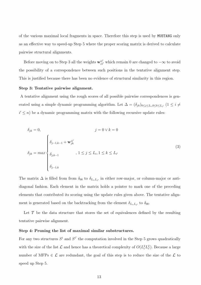
Step 3: Tentative pairwise alignment.

A tentative alignment using the rough scores of all possible pairwise correspondences is gen-

erated using a simple dynamic programming algorithm. Let ∆ = (δjk)0≤j≤Li,0≤k≤Li′(1 ≤ i 6=

i′ ≤ n) be a dynamic programming matrix with the following recursive update rules:

δjk = 0, j = 0 ∨ k = 0

δjk = max

δj−1,k−1 + wii′jk

δj,k−1

δj−1,k

, 1 ≤ j ≤ Li, 1 ≤ k ≤ Li′

(3)

The matrix ∆ is filled from from δ00 to δLi,Li′in either row-major, or column-major or anti-

diagonal fashion. Each element in the matrix holds a pointer to mark one of the preceding

elements that contributed its scoring using the update rules given above. The tentative align-

ment is generated based on the backtracking from the element δLi,Li′to δ00.

Let T be the data structure that stores the set of equivalences defined by the resulting

tentative pairwise alignment.

Step 4: Pruning the list of maximal similar substructures.

For any two structures Si and Si′ the computation involved in the Step 5 grows quadratically

with the size of the list L and hence has a theoretical complexity of O(L2i L

2i′). Because a large

number of MFPs ∈ L are redundant, the goal of this step is to reduce the size of the L to

speed up Step 5.

13

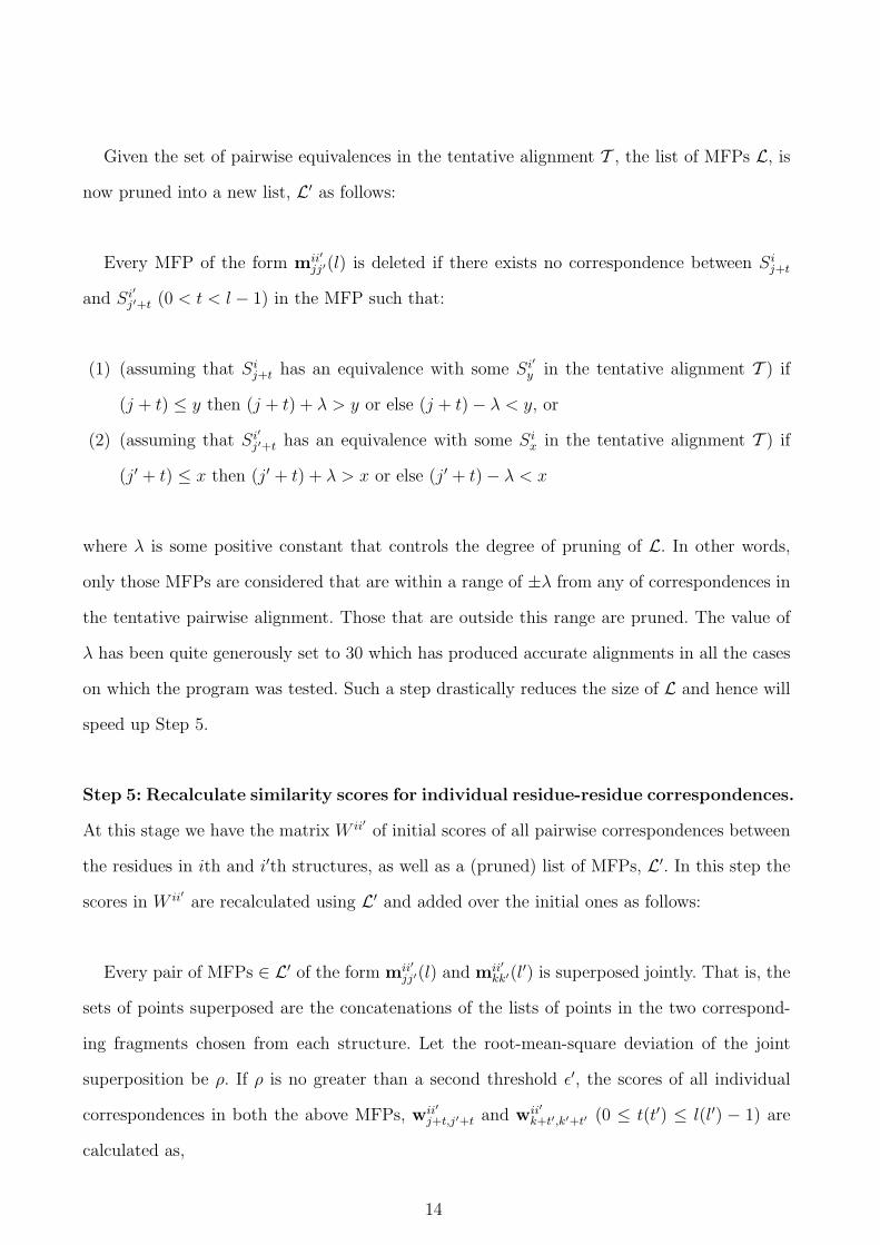
Given the set of pairwise equivalences in the tentative alignment T , the list of MFPs L, is

now pruned into a new list, L′ as follows:

Every MFP of the form mii′jj′(l) is deleted if there exists no correspondence between Si

j+t

and Si′j′+t (0 < t < l − 1) in the MFP such that:

(1) (assuming that Sij+t has an equivalence with some Si′

y in the tentative alignment T ) if

(j + t) ≤ y then (j + t) + λ > y or else (j + t)− λ < y, or

(2) (assuming that Si′j′+t has an equivalence with some Si

x in the tentative alignment T ) if

(j′ + t) ≤ x then (j′ + t) + λ > x or else (j′ + t)− λ < x

where λ is some positive constant that controls the degree of pruning of L. In other words,

only those MFPs are considered that are within a range of ±λ from any of correspondences in

the tentative pairwise alignment. Those that are outside this range are pruned. The value of

λ has been quite generously set to 30 which has produced accurate alignments in all the cases

on which the program was tested. Such a step drastically reduces the size of L and hence will

speed up Step 5.

Step 5: Recalculate similarity scores for individual residue-residue correspondences.

At this stage we have the matrix W ii′ of initial scores of all pairwise correspondences between

the residues in ith and i′th structures, as well as a (pruned) list of MFPs, L′. In this step the

scores in W ii′ are recalculated using L′ and added over the initial ones as follows:

Every pair of MFPs ∈ L′ of the form mii′jj′(l) and mii′

kk′(l′) is superposed jointly. That is, the

sets of points superposed are the concatenations of the lists of points in the two correspond-

ing fragments chosen from each structure. Let the root-mean-square deviation of the joint

superposition be ρ. If ρ is no greater than a second threshold ε′, the scores of all individual

correspondences in both the above MFPs, wii′j+t,j′+t and wii′

k+t′,k′+t′ (0 ≤ t(t′) ≤ l(l′) − 1) are

calculated as,

14

wii′j+t,j′+t = wii′

j+t,j′+t + (ε′ − ρ)2 ×

∑0≤p≤l−1

∑0≤q≤l′−1

φ(i, i′, j, j′, k, k′, p, q)

+∑

0≤q≤l′−1

φ(i, i′, j, j′, k, k′, t, q)

wii′k+t′,k′+t′ = wii′

k+t′,k′+t′ + (ε′ − ρ)2 ×

∑0≤p≤l−1

∑0≤q≤l′−1

φ(i, i′, j, j′, k, k′, p, q)

+∑

0≤p≤l−1

φ(i, i′, j, j′, k, k′, p, t′)

(4)

where φ(i, i′, j, j′, k, k′, x, y) in this step is calculated slightly differently from Equation 2 as,

φ(i, i′, j, j′, k, k′, x, y) =

θ −

∣∣∣dij+x,k+y−di′

j′+x,k′+y

∣∣∣d∗

× ω(d∗), cond1

θ, otherwise

(5)

where cond1 ≡ (j + x) 6= (k + y) ∧ (j′ + x) 6= (k′ + y), d∗ =

(di

j+x,k+y+di′j′+x,k′+y

2

), the constant

θ, distance dijk, and the envelope function ω have the same definitions as used in Equation 2.

For increased accuracy we avoid joint superpositions of any two MFPs that have in common

more than 80% of either of the fragments. This constraint prevents accumulation of unnecessary

weights.

The value of ε′ has been quite liberally fixed at 6.5. This generous threshold in conjunction

with the quadratic reward factor (ε′ − ρ)2 in equation 4 gives MUSTANG its ability to align

efficiently structures with conformational changes.

15

2.2.2 Phase 2: Gathering equivalences between residues from all pairs of structures in the

ensemble (Pairwise structural alignments)

Pairwise structural alignments are generated here using the scoring matrix W ii′ (∀1 ≤ i < i′ ≤

n). The dynamic programming method discussed in §2.2.1(Step 3) with update rules shown

in Equation 3 is used again. Let P ii′ be the data structure created by storing the equivalences

derived through every pairwise alignment in the ensemble.

2.2.3 Phase 3: Recalculation of scores of residue-residue correspondences in the context of

multiple structures (Extension phase)

The progressive pairwise alignment approach for constructing multiple alignments involves

merging a series of pairwise alignments along a guide tree. A lot of incorrect greedy choices are

made in such a procedure. Also, the order in which the pairwise alignments are forced affects

the accuracy and quality of the final multiple alignment. The extension phase used in MUSTANG

helps reduce the number of greedy choices made in the final progressive pairwise alignment

phase. The strategy MUSTANG uses is close in spirit to the ones used previously in sequence

comparison methods such as Notredame et al. [9], Morgenstern [60], and Neuwald et al. [61]

but the details of the procedure differ significantly.

A new matrix Wii′

= (wii′jj′)1≤j≤Li,1≤j′≤Li′

(1 ≤ i 6= i′ ≤ n) is generated in this phase

containing scores for every possible residue-residue correspondence between the two structures.

The scores at the start are initialised to zero. First, for every equivalence between the residues

Six and Si′

y in the pairwise alignment P ii′ we assign wii′xy = wii′

xy.

We next establish transitive correspondences between every pair of structures Si and Si′

(1 ≤ i 6= i′ ≤ n) through all possible intermediate structures Sj (1 ≤ j 6= i ∧ j 6= i′ ≤ n).

Given any equivalence between Six and Si′

y (or a gap) ∈ P ii′ , let Six be equivalent to Sj

z (and

not equivalent to a gap) in P ij, and let Sjz in turn be equivalent to Si′

y′ (and not equivalent

to a gap) in Pji′ , then we say that there is a (transitive) correspondence between Six and Si′

y′

through the intermediate Sjz . The score of the transitive correspondence, wii′

xy′ is calculated

16

as, †

wii′

xy′ = max(wii′

xy,wii′

x′y′

), Si

x ≡ Si′

y ∧ Si′

y′ ≡ Six′ ∧wii′

xy′ < max(wii′

xy,wii′

x′y′

)(6)

wii′

xy′ = wii′

xy , Six ≡ Si′

y ∧ Si′

y′ ≡ gap ∧wii′

xy′ < wii′

xy (7)

wii′

xy′ = wii′

x′y′ , Six ≡ gap ∧ Si′

y′ ≡ Six′ ∧wii′

xy′ < wii′

x′y′ (8)

wii′

xy′ = 1 , Six ≡ gap ∧ Si′

y′ ≡ gap ∧wii′

xy′ < 1 (9)

wii′

xy′ = wii′

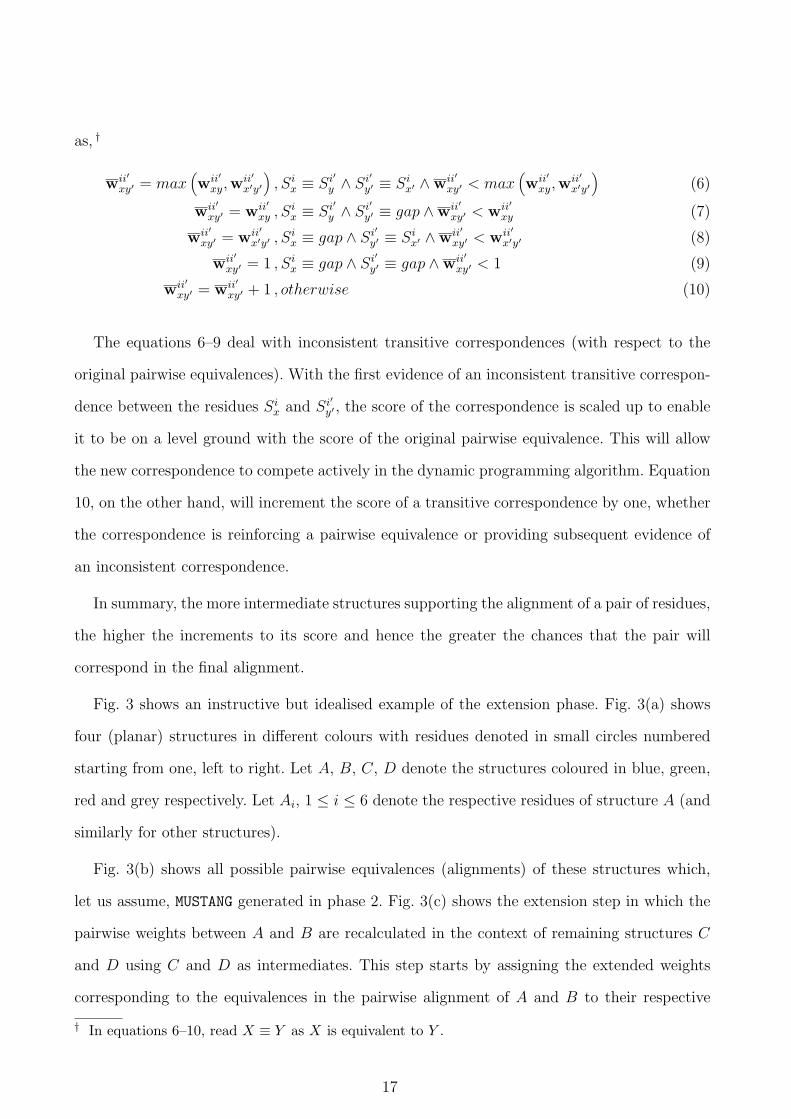
xy′ + 1 , otherwise (10)

The equations 6–9 deal with inconsistent transitive correspondences (with respect to the

original pairwise equivalences). With the first evidence of an inconsistent transitive correspon-

dence between the residues Six and Si′

y′ , the score of the correspondence is scaled up to enable

it to be on a level ground with the score of the original pairwise equivalence. This will allow

the new correspondence to compete actively in the dynamic programming algorithm. Equation

10, on the other hand, will increment the score of a transitive correspondence by one, whether

the correspondence is reinforcing a pairwise equivalence or providing subsequent evidence of

an inconsistent correspondence.

In summary, the more intermediate structures supporting the alignment of a pair of residues,

the higher the increments to its score and hence the greater the chances that the pair will

correspond in the final alignment.

Fig. 3 shows an instructive but idealised example of the extension phase. Fig. 3(a) shows

four (planar) structures in different colours with residues denoted in small circles numbered

starting from one, left to right. Let A, B, C, D denote the structures coloured in blue, green,

red and grey respectively. Let Ai, 1 ≤ i ≤ 6 denote the respective residues of structure A (and

similarly for other structures).

Fig. 3(b) shows all possible pairwise equivalences (alignments) of these structures which,

let us assume, MUSTANG generated in phase 2. Fig. 3(c) shows the extension step in which the

pairwise weights between A and B are recalculated in the context of remaining structures C

and D using C and D as intermediates. This step starts by assigning the extended weights

corresponding to the equivalences in the pairwise alignment of A and B to their respective

† In equations 6–10, read X ≡ Y as X is equivalent to Y .

17

pairwise weights. Let the thickness of black lines in the alignment be a visual representation

of their weights. The pairwise weights of A and B are first extended using C. We have A2

equivalent to C1 in the pairwise alignment of A and C, and C1 equivalent to B2 in the pairwise

alignment of B and C. Then the transitive correspondence between A2 and B2 is established.

In this case the transitive correspondence reinforces the original pairwise equivalence between

A2 and B2 in the pairwise alignment of A and B and hence the extended weight of this

correspondence is incremented by one (Equation 10) as reflected in the increase in the thickness

of the corresponding black line in the Figure. The weight between A3 and B3 is incremented

similarly through C2.

In contrast, the transitive correspondence between A4 and B4 through C3 is inconsistent

with the pairwise equivalence between A4 and gap in the pairwise alignment of A and B. Hence,

a correspondence between A4 and B4 is established with a weight equal to the weight of the

original pairwise equivalence between B4 and A5 (Equation 8). The inconsistent transitive

correspondence between A5 and B5 (through the intermediate C4) is assigned the maximum

of the weights of the pairwise equivalences, A5 ≡ B4 and B5 ≡ A6 (Equation 6).

Having extended the pairwise weights between A and B through the intermediate C, we now

extend the same weights using D as the intermediate structure. The transitive correspondences

A1 ≡ B1 (through D1), A2 ≡ B2 (through D2), and A3 ≡ B3 (through D3) are all consistent

with the original pairwise alignments; hence the corresponding weights are incremented by

one as before. In this case again, the transitive correspondences A4 ≡ B4 (through D4), and

A5 ≡ B5 (through D5) are inconsistent with the equivalences from the pairwise alignment.

However, we had already encountered these (transitive) correspondences during the previous

extension through C, hence the corresponding extended weights are merely incremented by

one in these cases. By the end of all the extensions, we now have a new scoring matrix for

A and B with weights that reflect the information of equivalences from other structures (C

and D) in the ensemble. Such extensions are undertaken for all pairs before using these new

extended weights in the final progressive alignment stage.

[Fig. 3 about here.]

18

The computation in this phase grows as O(n3l2) (l = max(L1, · · · , Ln)).

2.2.4 Phase 4: Progressive alignment phase

The progressive alignment phase involves finding a guide tree along which the final multiple

alignment is constructed [8, 62]. The problem of building the phylogenetic tree of proteins

based on structural information is still an open problem [37]. But at this step we merely aim

to generate a quick and practical guide tree in order to align the structures.

In order to calculate a distance-divergence matrix K, the normalised alignment score of each

pairwise (structural) alignment, ζii′ (∀1 ≤ i ≤ i′ ≤ n), is first calculated using the equivalences

in the pairwise alignment P ii′ as,

ζii′ =∑

(j,j′)∈Pii′

wii′

jj′ ×maxcond1

(wkk′

ll′

)maxcond2

(wii′

ll′

)

where cond1 ≡ ((∀1 ≤ k < k′ ≤ n) ∧ (∀1 ≤ l ≤ Lk) ∧ (∀1 ≤ l′ ≤ Lk′)), and

cond2 ≡ ((∀1 ≤ l ≤ Li) ∧ (∀1 ≤ l′ ≤ Li′)) .

The similarity score ζii′ is then transformed into a distance divergence score Kii′ as,

Kii′ = − ln

(ζii′

max1≤j<j′<n ζjj′

).

The binary guide tree is constructed using the neighbour-joining method [63] applied to the

distance divergence matrix, K. In the final alignment stage, alignments are forced between two

clusters of sub-alignments. In MUSTANG we use a profile function calculated as the sum of scores

of all pairwise correspondences (SP) between any two columns in the two sub-alignments:

SP xy =∑i,j∈x

∑i′,j′∈y

(wii′

jj′

)

where, x and y are two columns of alignments – one from each cluster – that are to be joined

together, i(i′), j(j′) are the indices of the structure and the position of the residue in the chain

respectively.

The result is a multiple alignment. From the correspondences in the multiple alignment, all

19

the structures are optimally superposed on each other using the method described in Diamond

[55], applied to the subset of positions occupied in all sequences by genuine residues (that is,

the set of positions for which no sequence contains a gap.)

2.3 Implementation of MUSTANG

The MUSTANG algorithm has been implemented using a conservative subset of C++. The

experiments on various data sets were conducted on a Fedora Core 3 Linux platform with

1.2GHz CPU and 256 MB primary memory. The speed of the program depends on the following

factors:

(1) The number of input structures in the ensemble.

(2) The sizes of input structures

(3) The sizes of the maximal fragment pairs list.

For example, the 11 Set 3 globin structures given in the Table I in §3.1.1 took 133 s to align.

The command line program (including its source) is available from http://www.cs.mu.oz.

au/~arun/mustang. The program accepts as input coordinates in PDB format. MUSTANG reports

the alignment of sequences in an HTML format (appearing as in Fig. 1(b)) and optionally in

many other formats. It also generates as output the structures brought to a common coordinate

frame in which they are optimally superposed based on the multiple alignment.

3 Results and Discussion

3.1 Tests of MUSTANG alignments and comparison with other programs

The performance of MUSTANG was tested on numerous data sets. Several published align-

ments were used in the evaluation. Of particular interest are tests on difficult cases, involving

very highly-diverged proteins or structures which show conformational flexibilities. MUSTANG’s

performance was also compared with POSA [37], CE-MC [35], MultiProt [42], and MALECON [64]

using our selected data sets as well as those described in the relevant papers. All the HOMSTRAD

20

alignment families were aligned using MUSTANG and comparisons were made with the database

benchmarks. Finally, because the reliability of MUSTANG is based on its pairwise structural

alignments, and because DALI is widely considered to represent the state of the art in pairwise

structural alignment, we compared the results of MUSTANG and DALI over 633 HOMSTRAD families

containing only two structures per family.

3.1.1 Comparisons with curated alignments

We ran MUSTANG on several data sets for which manually generated alignments are available.

Globins: The globins are one of the most extensively-studied protein families. Lesk and

Chothia [21] reported a manually-generated alignment of globin structures then available.

These proteins were realigned using MUSTANG.

For these tests, the structures used were grouped into three sets, corresponding to different

degrees of divergence. Set 1 contains mammalian globins only: the α and β subunits of human

and horse haemoglobin, and sperm whale myoglobin. Set 2 contains all the structures treated

in the 1980 work, extending Set 1 by the inclusion of invertebrate and plant globins. Since

1980, the globin family has grown considerably. In particular, a set of truncated globins from

microorganisms has been discovered, and some of the structures solved and their sequences

aligned with the full-length globins [65, 66]. Table I contains the PDB codes of these three sets

of structures.

[Table I about here.]

MUSTANG’s alignments of these Globin data sets can be found at http://www.cs.mu.oz.au/

~arun/mustang/globins.html.

The alignment of all the three sets agrees with the published alignments described in Lesk

and Chothia [21] and Lesk [65] except for a few minor disagreements which are only in regions of

dissimilar conformation where it is difficult to align with confidence. The inclusion of additional

structures in Set 2 over Set 1 did not affect the alignment of common structures. However the

alignment of the Set 2 structures in the Set 2 alignment was slightly better, in some regions,

21

than the alignment of the Set 2 structures within the Set 3 (= Set 2 + three truncated globins)

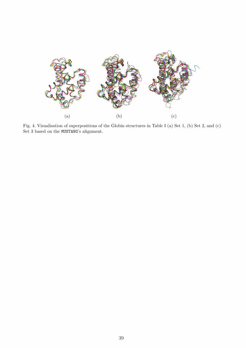
alignment, suggesting in this case, some deterioration. Fig. 4 shows the superpositions of the

structures based on the alignments of the above sets. Comparison with Fig. 1(a) shows that the

conserved core of the full-length globins comprises an unusually high portion of the structure.

[Fig. 4 about here.]

Serine Proteinases: MUSTANG was run on the Serine proteinase data sets shown in Table I

and compared with the published alignments in Lesk and Fordham [48]. Again, Set 1 contains

a relatively closely-related group of mammalian serine proteinases, and Set 2 contains a more

widely-diverged set of mammalian and bacterial serine proteinases. (Because of horizontal

gene transfer, Streptomyces griseus trypsin is effectively a mammalian protein.) MUSTANG’s

alignments of the above data sets can be found at http://www.cs.mu.oz.au/~arun/mustang/

serine_prot.html. For Set 1, we observe that all the positions in the Lesk and Fordham [48]

alignment that are occupied by a residue (not a gap) in every sequence are identically aligned

by MUSTANG. The published alignment has 174 columns/positions which are ungapped whereas

MUSTANG’s alignment has 205 such positions. Note the large difference between the programs

in choosing when to align and when not to. In almost all the regions of the alignments where

there are disagreements, MUSTANG’s alignment is preferable.

In Set 2, the published alignment has 63 ungapped positions whereas MUSTANG’s alignment

produced 119 such positions in its alignment, consistent with the suggestion that the published

alignment is more conservative than MUSTANG in assigning equivalences. However, with a few

exceptions, most of the ungapped columns in the published alignment are the same in MUSTANG’s

alignment. Fig. 5(a), and (b) show the superpositions of these two sets according to the MUSTANG

alignments.

[Fig. 5 about here.]

As in the case of the globins, we also compared the effect of inclusion of additional structures

in Set 2 on the alignment of the structures common to Set 1 and Set 2. In doing so we not

only evaluate the performance of MUSTANG on these examples but also ask how stable MUSTANG

is with respect to the addition of more structures to the ensemble. At almost all positions,

22

MUSTANG produced alignments in which the structures common to both sets are equivalently

aligned. Almost all of the differences we observe are very minor shifts in noisy regions. In this

case the additional structures in Set 2 neither improve the alignment of the Set 1 structures

nor degrade the quality of their separate alignment.

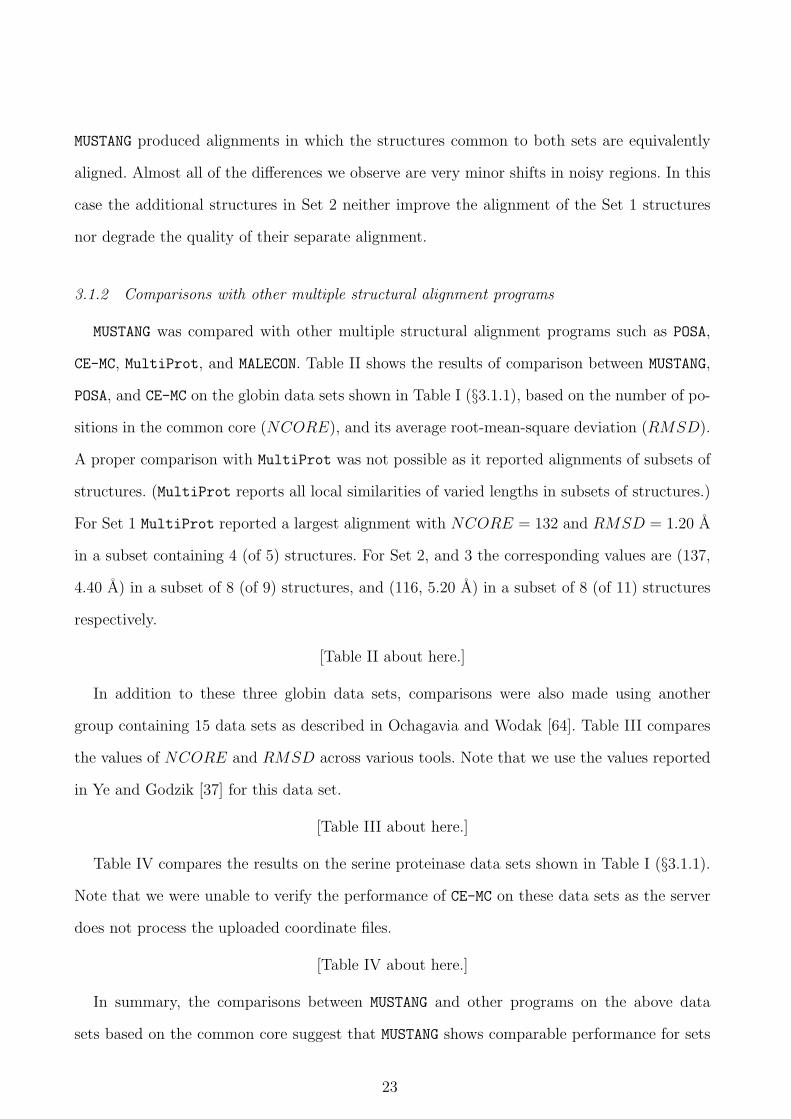
3.1.2 Comparisons with other multiple structural alignment programs

MUSTANG was compared with other multiple structural alignment programs such as POSA,

CE-MC, MultiProt, and MALECON. Table II shows the results of comparison between MUSTANG,

POSA, and CE-MC on the globin data sets shown in Table I (§3.1.1), based on the number of po-

sitions in the common core (NCORE), and its average root-mean-square deviation (RMSD).

A proper comparison with MultiProt was not possible as it reported alignments of subsets of

structures. (MultiProt reports all local similarities of varied lengths in subsets of structures.)

For Set 1 MultiProt reported a largest alignment with NCORE = 132 and RMSD = 1.20 A

in a subset containing 4 (of 5) structures. For Set 2, and 3 the corresponding values are (137,

4.40 A) in a subset of 8 (of 9) structures, and (116, 5.20 A) in a subset of 8 (of 11) structures

respectively.

[Table II about here.]

In addition to these three globin data sets, comparisons were also made using another

group containing 15 data sets as described in Ochagavia and Wodak [64]. Table III compares

the values of NCORE and RMSD across various tools. Note that we use the values reported

in Ye and Godzik [37] for this data set.

[Table III about here.]

Table IV compares the results on the serine proteinase data sets shown in Table I (§3.1.1).

Note that we were unable to verify the performance of CE-MC on these data sets as the server

does not process the uploaded coordinate files.

[Table IV about here.]

In summary, the comparisons between MUSTANG and other programs on the above data

sets based on the common core suggest that MUSTANG shows comparable performance for sets

23

of relatively closely-related proteins, and performs better in difficult cases containing very

distantly-related proteins (such as Set 3 of Globins and Set 2 of Serine proteinases).

MUSTANG was compared with POSA on structures that contain structural flexibilities in which

POSA performs largely better than other available programs. We treated the two data sets

on which POSA’s performance has been documented: Calmodulin-like proteins and tRNA syn-

thetases.

On the Calmodulin-like data set containing 3 structures (PDB codes: 1jfj, chain a; 1ncx;

2sas) MUSTANG was able to detect a common core of length 129 positions. The alignment

results can be found at http://www.cs.mu.oz.au/~arun/mustang/Calmodulin.html. POSA

on the other hand detected a common core of 132 positions. Although the alignments were

comparable, there is a difference in the superposition facilities of MUSTANG and POSA. POSA

incorporates structural flexibility into its superposition; MUSTANG, in its current form does

not. (Such a feature will be added to the program shortly.) Therefore Fig. 6(a), showing

the overall superposition MUSTANG generated, is unsatisfactory. Fig. 6(b) shows the individual

superpositions of each of the two domains generated using MUSTANG’s alignment of the entire

proteins.

[Fig. 6 about here.]

For the four tRNA synthetase structures used in POSA (PDB codes: 1adj, 1hc7, 1qf6, and

1ati), MUSTANG found 291 aligned positions as the common core of its alignment compared

with 278 positions in POSA. Fig. 7(a) shows the global superposition of the tRNA synthetases

MUSTANG generated. Fig. 7(b) show the individual superpositions of the region around the

common core in domain 1 and domain 2.

[Fig. 7 about here.]

The results of the calmodulin-like, and tRNA synthetase data sets suggests that MUSTANG

is robust and comparable to POSA in the alignments it produces in cases where the data sets

have structural flexibility.

24

3.1.3 MUSTANG’s performance on HOMSTRAD families

HOMSTRAD is a database of protein structural alignments for homologous families [67]. Its

alignments were generated using structural alignment programs such as MNYFIT, STAMP

and COMPARER followed by a manual scrutiny of individual cases. The performance of

MUSTANG was compared with the database of 1033 HOMSTRAD families. The alignment results

along with the superposed coordinates can be found at http://www.cs.mu.oz.au/~arun/

mustang/homstrad.html.

The alignment accuracy (ACC) metric was used for comparison with HOMSTRAD. ACC is

calculated by comparing every possible imposed pairwise alignment in the query (MUSTANG)

multiple alignment against the corresponding imposed pairwise alignment in the reference

(HOMSTRAD) alignment. All correctly aligned residue pairs in comparison with the reference are

considered as hits and those that disagree as errors. The percentage of correctly aligned residues

in every pairwise alignment is then calculated and the mean of these pairwise accuracies is used

as the accuracy, ACC, of the query multiple alignment with respect to the reference.

The mean ACC over all 1033 data sets is 93.4%. In general MUSTANG alignments gave smaller

common cores when compared to the database alignments, and, concomitantly, slightly lower

RMSDs.

3.2 Comparisons with DALI at a pairwise level

MUSTANG, at a pairwise level, was compared to DALI which is widely considered to be the

best of the available pairwise structural alignment tools. For this comparison we used the 633

HOMSTRAD alignment families containing two structures per family.

The metric ACC defined in the previous section (§3.1.3) was used to compare MUSTANG-

with-HOMSTRAD, DALI-with-HOMSTRAD (both using the HOMSTRAD alignment as reference), and

MUSTANG-with-DALI (using the DALI alignment as reference).

The average alignment accuracies of the above three comparisons averaged over 633 HOMSTRAD

alignment families are 93.9%, 92.6%, and 87.8% respectively. The results show that MUSTANG

25

and DALI have comparable performances when comparing their alignments to HOMSTRAD.

MUSTANG agrees with HOMSTRAD slightly better than DALI does. To compare the performance

of MUSTANG and DALI specialised to a specific type of secondary structure we extracted all-α

and all-β families from HOMSTRAD. MUSTANG and DALI shared 88.4 % and 86.6 % of aligned

residues in common, averaged over all families in all-α and all-β sets respectively. Notice that

these values do not differ significantly from the average over all 633 HOMSTRAD families. This

indicates that the two methods perform with comparable accuracy on regions containing these

two types of secondary structures.

We also compared the alignments produced by MUSTANG and DALI for many pairs of homol-

ogous proteins, over a range of similarity. In a vast majority of the cases the alignments agree,

either completely, or to within a few minor differences involving small shifts in few residues.

Often it is a question of precisely where to insert a necessary gap.

In a number of cases where the two methods gave significantly different alignments, we

examined the alternative superpositions of the relevant substructures in detail. Many of the

differences appear in ill-fitting, noisy regions where it is not objectively possible to decide

which of the two alignments is better. In some cases we think that DALI’s alignment of certain

regions is correct and MUSTANG’s is wrong; in a comparable number of other cases we think

that MUSTANG’s alignment is correct and DALI’s is wrong; in a few cases we feel that neither

program gets the alignment quite right. We did not check by hand the very large number of

regions in which MUSTANG and DALI agree, although it is possible that we might not accept

their common answer in all cases.

As MUSTANG and DALI share in common 87.8% of their respective alignments (on a residue-

position basis averaged over 633 HOMSTRAD families), MUSTANG and DALI agree far more than

they disagree.

MUSTANG is more conservative than DALI in deciding whether to align residues or to declare

them unalignable. In other words, MUSTANG tends to introduce more gaps into its alignments

than DALI does. Averaged over 633 HOMSTRAD families, MUSTANG inserts 4.44% more gaps than

DALI. Recall that in structural alignment the notion of what can or cannot be aligned is not well

26

defined (Irving et al. [14]). Any program can be set to align more or fewer residues by adjusting

parameters that control its degree of tolerance to conformational differences. Therefore we do

not regard the overall difference in the % gaps introduced in the alignments as any measure of

the quality of the alignments produced by MUSTANG and DALI.

In conclusion, we do not suggest that MUSTANG should replace DALI for pairwise alignment.

But neither would we advise against using MUSTANG for pairwise alignment. If we wished

to determine a structural alignment of two proteins, we would run both DALI and MUSTANG,

compare the results, and inspect any differences by drawing pictures.

3.3 Comparisons of sequence-based and structural alignments in cases in which they are in

conflict

The examples in this section reflect and emphasise the differences between alignments based

purely on sequences, and structural alignments. They include examples of closely related se-

quences of proteins that contain structurally-dissimilar regions.

3.3.1 Domain swapping: Odorant-binding proteins

Pig odorant-binding protein (PDB code: 1a3y) is a monomer containing in its C-terminal

segment a helix and a strand of sheet (shown in red in Fig. 8(a)). Cow odorant-binding protein

(PDB code: 1obp) is a dimer (shown in Olive and Pink in Fig. 8(b)) in which the C-terminal

helix and strand of each monomer flip over to interact with the partner (shown in Green and

Red in Fig. 8(b)) [68].

Fig. 8(c) shows the sequence alignment (generated using ClustalW [8]) and structural align-

ment (generated using MUSTANG) of the two odorant-binding proteins. The sequences of the two

proteins are very similar. In the alignment based solely on the sequences, the monomer (1a3y)

is aligned with one of the monomers of 1obp. However the aligned C-terminal segments of the

two proteins do not occupy the same positions in space (See Fig. 8(d)). A structural alignment

that matches residues occupying equivalent positions in space generates an alignment that

differs in the region of the domain swap (Fig. 8(e)).

27

[Fig. 8 about here.]

3.3.2 Bacterial Lipases

The HOMSTRAD family Bacterial Lipase (bac lipase) contains two proteins with very closely

related sequences:

(1) lipase (triacylglycerol lipase) from Chromobacterium viscosum (PDB code: 1cvl)

(2) lipase precursor (triacylglycerol lipase) from Burkholderia cepacia (PDB code: 4lip, chain

d)

Fig. 9 shows the alignments of these proteins by HOMSTRAD and MUSTANG, in the region in which

they disagree, and the superposition of the structures in this region. Outside this region the

HOMSTRAD and MUSTANG alignments are in total agreement with each other.

[Fig. 9 about here.]

From a perspective of the evolutionary relationship of these sequences, HOMSTRAD has cor-

rectly aligned the residues in this region, which are almost identical. Despite the similarity of

sequences, however, the structures of the region are different (see Fig. 9(b)). Any structural

alignment method will insert some gaps in this regions, as MUSTANG does. This is not a case

of such widely-diverged proteins that sequence alignment will be untrustworthy, but rather a

case where there is a choice between an alignment based purely on sequences, and a struc-

tural alignment. The two alignments are complementary: by comparing them, one’s attention

is called to the structural difference.

The implication is that, in choosing sequence or structural alignment, the user must pay

attention to the purpose of the calculation and the intended use of the result. It is a case of

‘Be careful what you ask for, you might get it.’

4 Conclusions

We have designed, written, and tested an algorithm for multiple structural alignment of

proteins. The program is robust, fully automatic, efficient and easy to use. The performance

28

of MUSTANG compares favourably with published multiple structural alignment programs, and

indeed is more reliable than others on hard data sets.

References

[1] Read RJ. Pushing the boundaries of molecular replacement with maximum likelihood.

Acta Cryst., 2001, D57:1373–1382.

[2] Storoni LC, McCoy AJ, Read RJ. Likelihood-enhanced fast rotation functions. Acta

Cryst., 2004, D60:432–438.

[3] Schwarzenbacher R, Godzik A, Grzechnik SK, Jaroszewski L. The importance of alignment

accuracy for molecular replacement. Acta Cryst., 2004, D60:1229–1236.

[4] Altschul SF, Madden TL, Schaeffer AA, Zhang J, Zhang Z, Miller W, Lipman DJ. Gapped

BLAST and PSI-BLAST: A new generation of protein database search programs. Nucleic

Acids Res., 1997, 25:3389–3402.

[5] Needleman SB, Wunsch CD. A general method applicable to the search for similarities in

amino acid sequence of two proteins. J. Mol. Biol., 1970, 48:443–453.

[6] Smith TF, Waterman MS. Identification of common molecular subsequences. J. Mol.

Biol., 1981, 147:195–197.

[7] Altschul SF, Gish W, Miller W, Myers EW, Lipman DJ. Basic local alignment search

tool. J. Mol. Biol., 1990, 215:403–410.

[8] Thompson JD, Higgins DG, Gibson TJ. CLUSTAL W: Improving the sensitivity of

progressive multiple alignment through sequence weighting, position-specific gap penalties

and weight matrix choice. Nucleic Acids Res., 1994, 22:4673–4680.

[9] Notredame C, Higgins D, Heringa J. T-Coffee: A novel method for multiple sequence

alignments. J. Mol. Biol., 2000, 302:205–217.

[10] Edgar RC. MUSCLE: Multiple sequence alignment with high accuracy and high through-

put. Nucleic Acids Res., 2004, 32:1792–1797.

[11] Notredame C. Recent progress in multiple sequence alignments: A survey. Pharmacoge-

nomics, 2002, 3:1–14.

29

[12] Holm L, Sander C. Protein structure comparison by alignment of distance matrices. J.

Mol. Biol., 1993, 233:123–138.

[13] Chothia C, Lesk AM. The relationship between the divergence of sequence and structure

in proteins. EMBO J., 1986, 5:823–826.

[14] Irving JA, Whisstock JC, Lesk AM. Protein structural alignments and functional ge-

nomics. Proteins: Struct. Funct. Gen., 2001, 42:378–382.

[15] Sali A, Blundell TL. Definition of general topological equivalence in protein structures.

A procedure involving comparison of properties and relationships through simulated an-

nealing and dynamic programming. J. Mol. Biol., 1990, 212:403–428.

[16] Pearce M, Bottomley S, Pike R, Lesk A. In: Lomas D, Silverman G, editors. Molecular and

Cellular Aspects of the Serpinopathies and Disorders in Serpin Activity. World Scientific,

Singapore, 2006.

[17] Levine M, Stuart D, Williams J. A method for systematic comparison of the three-

dimensional structures of proteins and some results. Acta Cryst., 1984, A40:600–610.

[18] Karpen ME, de Haseth PL, Neet KE. Comparing short protein substructures by a method

based on backbone torsion angles. Proteins: Struct. Funct. Gen., 1989, 6:155–167.

[19] Lesk AM. Computational molecular biology. In: Kent A, Williams JG, editors. Encyclo-

pedia of Computer Science and Technology, volume 31. Marcel Dekker, New York, USA.,

1994, p 101–165.

[20] Caprara A, Carr R, Istrail S, Lancia G, Walenz B. 1001 optimal pdb structure alignments:

integer programming methods for finding the maximum contact map overlap. J. Comput.

Biol., 2004, 11:27–52.

[21] Lesk AM, Chothia C. How different amino acid sequences determine similar protein

structures: I. The structure and evolutionary dynamics of the globins. J. Mol. Biol., 1980,

136:225–270.

[22] Lesk AM. 11th Lipari international summer school in computational biology, 1999.

[23] McLachlan AD. A mathematical procedure for superimposing atomic coordinates of pro-

teins. Acta Cryst., 1972, A28:656.

30

[24] Kabsch W. A solution for the best rotation to relate two sets of vectors. Acta Cryst.,

1976, A32:922–923.

[25] Kearsley SK. On the orthogonal transformation used for structural comparisons. Acta

Cryst., 1989, A45:208–210.

[26] Rustici M, Lesk AM. Three-dimensional searching for recurrent structural motifs in

databases of protein structures. J. Comput. Biol., 1994, 1:121–132.

[27] Orengo CA, Taylor WR. A rapid method for protein structure alignment. J. Theor. Biol.,

1990, 147:517–551.

[28] Gerstein M, Levitt M. Using iterative dynamic programming to obtain accurate pairwise

and multiple alignments of protein structures. In Proceedings of the Fourth International

Conference on Intelligent Systems for Molecular Biology. AAAI Press, USA, 1996, p 59–

67.

[29] Nussinov R, Wolfson HJ. Efficient detection of three-dimensional structural motifs in

biological macromolecules by computer vision techniques. Proc. Natl. Acad. Sci. USA,

1991, 88:10495–10499.

[30] Koehl P. Protein structure similarities. Curr. Opin. Struct. Biol., 2001, 11:348–353.

[31] Just W. Computational complexity of multiple sequence alignment with SP-score. J.

Comput. Biol., 2001, 8:615–623.

[32] Wang L, Jiang T. On the complexity of multiple sequence alignment. J. Comput. Biol.,

1994, 1:337–348.

[33] Goldman D, Papadimitriou CH, Istrail S. Algorithmic aspects of protein structure similar-

ity. In FOCS ’99: Proceedings of the 40th Annual Symposium on Foundations of Computer

Science. IEEE Computer Society, Washington, DC, USA, 1999, p 512.

[34] Guda C, Scheeff ED, Bourne PE, Shindyalov IN. A new algorithm for the alignment of

multiple protein structures using Monte Carlo optimization. In Pacific Symposium on

Biocomputing, 2001, p 275–286.

[35] Guda C, Lu S, Scheeff ED, Bourne PE, Shindyalov IN. CE-MC: A multiple protein

structure alignment server. Nucleic Acids Res., 2004, 32:100–103.

31

[36] Shindyalov IN, Bourne PE. Protein structure alignment by incremental combinatorial

extension (CE) of the optimal path. Protein Eng., 1998, 11:739–747.

[37] Ye Y, Godzik A. Multiple flexible structure alignment using partial order graphs. Bioin-

formatics, 2005, 21:2362–2369.

[38] Lee C, Grasso C, Sharlow MF. Multiple sequence alignment using partial order graphs.

Bioinformatics, 2002, 18:452–464.

[39] Ye Y, Godzik A. Flexible structure alignments by chaining aligned fragment pairs allowing

twists. Bioinformatics, 2003, 19:II246–II255.

[40] Ye J, Janardan R. Approximate multiple protein structure alignment using the sum-of-

pairs distance. J. Comput. Biol., 2004, 11:986–1000.

[41] Gusfield D. Efficient methods for multiple sequence alignment with guaranteed error

bounds. Bull. Math. Biol., 1993, 55:141–154.

[42] Shatsky M, Nussinov R, Wolfson H. MULTIPROT- A multiple protein structural align-

ment algorithm. In: Guigo R, Gusfield D, editors. Workshop on Algorithms in Bioinfor-

matics, volume 2452 of Lect. Notes Comp. Sci. Springer-Verlag, Berlin, 2002, p 235–250.

[43] Dror O, Benyamini H, Nussinov R, Wolfson HJ. Multiple structural alignment by sec-

ondary structures: Algorithm and applications. Protein Sci., 2003, 12:2492–2507.

[44] Leibowitz N, Nussinov R, Wolfson HJ. MUSTA - A general, efficient, automated method

for multiple structure alignment and detection of common motifs: Application to proteins.

J. Comput. Biol., 2001, 8:93–121.

[45] Russell R, Barton G. Multiple protein sequence alignment from tertiary structure com-

parison: assignment of global and residue confidence levels. Proteins: Struct. Funct. Gen.,

1992, 14:309–323.

[46] Sutcliffe MJ, Haneef I, Carney D, Blundell TL. Knowledge based modelling of homologous

proteins. Part I: Three-dimensional frameworks derived from the simultaneous superposi-

tion of multiple structures. Protein Eng., 1987, 1:377–384.

[47] Lesk AM. Three-dimensional pattern matching in protein structure analysis. In: Galil Z,

Ukkonen E, editors. Combinatorial pattern matching, volume 937 of Lect. Notes Comp.

32

Sci. Springer-Verlag, Berlin, 1995, p 248–260.

[48] Lesk AM, Fordham WD. Conservation and variability in the structures of serine pro-

teinases of the chymotrypsin family. J. Mol. Biol., 1996, 258:501–537.

[49] Taylor WR, Flores TP, Orengo CA. Multiple protein structure alignment. Protein Sci.,

1994, 3:1858–1870.

[50] Taylor WR, Orengo CA. Protein structure alignment. J. Mol. Biol., 1989, 208:1–22.

[51] Ding DF, Qian J, Feng ZK. A differential geometric treatment of protein structure com-

parison. Bull. Math. Biol., 1994, 56:923–943.

[52] May ACW, Johnson MS. Improved genetic algorithm-based protein structure compar-

isons: pairwise and multiple superpositions. Protein Eng., 1995, 8:873–882.

[53] Eidhammer I, Jonassen I, Taylor WR. Protein Bioinformatics: An algorithmic approach

to sequence and structure analysis. J. Wiley Sons Ltd., Chichester, England, 2004.

[54] Shapiro A, Botha JD, Pastore A, Lesk AM. A method for multiple superposition of

structures. Acta Cryst., 1992, A48:11–14.

[55] Diamond R. On the multiple simultaneous superposition of molecular structures by rigid

body transformations. Protein Sci., 1992, 1:1279–1287.

[56] Maiorov VN, Crippen GM. Contact potential recognizes the correct folding of globular

proteins. J. Mol. Biol., 1992, 227:876–888.

[57] Crippen GM. Recognizing protein folds by cluster distance geometry. Proteins: Struct.

Funct. Gen., 2005, 60:82–89.

[58] Havel TF, Kuntz ID, Crippen GM. The theory and practice of distance geometry. Bull.

Math. Biol., 1983, 45:665–720.

[59] Richards FM, Kundrot CE. Identification of structural motifs from protein coordinate

data: secondary structure and first-level supersecondary structure. Proteins, 1988, 3:

71–84.

[60] Morgenstern B. Dialign2: Improvement of the segment-to-segment approach to multiple

sequence alignment. Bioinformatics, 1999, 15:211–218.

[61] Neuwald AF, Liu JS, Lipman DJ, Lawrence CB. Extracting protein alignment models

33

from the sequence database. Nucleic Acids Res., 1997, 25:1665–1677.

[62] Feng DF, Doolittle RF. Progressive sequence alignment as a prerequisite to correct phy-

logenetic trees. J. Mol. Evol., 1987, 25:351–360.

[63] Saitou N, Nei M. The neighbor-joining method: A new method for reconstructing phylo-

genetic trees. Mol. Biol. Evol., 1987, 4:406–425.

[64] Ochagavia ME, Wodak S. Progressive combinatorial algorithm for multiple structural

alignments: applications to distantly related proteins. Proteins: Struct. Funct. Bioinfo.,

2004, 55:436–454.

[65] Lesk AM. The evolution of the globins: We thought we understood it. In: Bastolla U, Porto

M, Roman HE, Vendruscolo M, editors. Structural Approaches to Sequence Evolution.

Springer-Verlag, Berlin, 2005.

[66] Vuletich DA, Lecomte JT, Lesk AM. Structural divergence and distant relationships in

proteins: evolution of the globins. Curr. Opin. Struct. Biol., 2005, 15:290–301.

[67] Mizuguchi K, Deane CM, Blundell TL, Overington JP. HOMSTRAD: A database of

protein structure alignments for homologous families. Protein Sci., 1998, 7:2469–2471.

[68] Ramoni R, Vincent F, Ashcroft AE, Accornero P, Grolli S, Valencia C, Tegoni M, Cam-

billau C. Control of domain swapping in bovine odorant-binding protein. Biochem. J.,

2002, 365:739–748.

34

List of Figures

1 (a) Multiple superposition of 3 small Copper-binding proteins: spinachplastocyanin (PDB code 1ag6), Alcaligenes denitrificans azurin (2aza) andcucumber stellacyanin (1jer). (1ag6–Cyan; 1jer–Green; 2aza–Magenta) basedon MUSTANG’s alignment. Regions aligned by MUSTANG’s alignment (see Fig. 1(b))are shown as thick ribbons. These prominently include the double−β−sheetstructure. The non-alignable regions are shown in thin lines. The respectiveCopper ions bound to the 3 proteins are shown at the top in large spheres.(b) Alignment of the Copper-binding proteins that MUSTANG produced. Coloursindicate the chemical nature of the amino acid. Red = small hydrophobicincluding aromatic; Blue = Acidic; Magenta = Basic; and Green = Basicamino acids with hydroxyl groups and/or amine groups. The ‘markup row’below each stretch of the multiple alignment indicates completely conservedresidues (in UPPERCASE) and partially-conserved residues (in lowercase) in acolumn of the alignment. 36

2 An overview of the MUSTANG algorithm. 37

3 An idealised example of the extension phase where weights are recalcu-lated(extended) for each pair, in the context of the multiple alignment. (a)Input (hypothetical) structures A (Blue), B (Green), C (Red), D (Gray);(b) Various pairwise alignments of the input structures; (c) illustration ofextension of pairwise correspondences between structure A and structure Busing structures C, and D as intermediates. 38

4 Visualisation of superpositions of the Globin structures in Table I (a) Set 1,(b) Set 2, and (c) Set 3 based on the MUSTANG’s alignment. 39

5 Visualisation of superpositions of the Serine proteinase structures in Table I(a) Set 1, and (b) Set 2 based on the MUSTANG’s alignment. 40

6 Visualisation of (a) global superposition based on MUSTANG’s alignment, (b)individual superpositions of the common core in first and second domainsrespectively based on the correspondences in the MUSTANG’s alignment, forthe three calmodulin-like proteins used in POSA. (1jfja–Red; 1ncx–Green;2sas–Blue) 41

7 Visualisation of (a) global superposition based on the MUSTANG’s alignment, (b)individual superpositions of the common core in domains 1 and 2 based onthe correspondences in the MUSTANG’s alignment, for the four tRNA synthetasestructures. (1adj–Red; 1ati–Green; 1hc7–Blue; 1qf6–Yellow) 42

8 Structures of (a) Pig odorant-binding protein (1a3y), and (b) Cowodorant-binding protein (1obp); (c) Sequence alignment using ClustalW, andStructural alignment using MUSTANG, of the two odorant-binding proteins; (d)superposition based on sequence alignment, and (e) superposition based onstructural alignment. 43

9 (a) The region in the bacterial lipase family where the HOMSTRAD and MUSTANG

alignments disagree; (b) A visualisation of the region in the alignment showingthe variability of the structures even though the sequences in this region arealmost identical. (1cvl–Yellow; 4lipd–Blue) 44

35

(a)

(b)

Fig. 1. (a) Multiple superposition of 3 small Copper-binding proteins: spinach plastocyanin (PDBcode 1ag6), Alcaligenes denitrificans azurin (2aza) and cucumber stellacyanin (1jer). (1ag6–Cyan;1jer–Green; 2aza–Magenta) based on MUSTANG’s alignment. Regions aligned by MUSTANG’s alignment(see Fig. 1(b)) are shown as thick ribbons. These prominently include the double−β−sheet structure.The non-alignable regions are shown in thin lines. The respective Copper ions bound to the 3 proteinsare shown at the top in large spheres. (b) Alignment of the Copper-binding proteins that MUSTANGproduced. Colours indicate the chemical nature of the amino acid. Red = small hydrophobic includingaromatic; Blue = Acidic; Magenta = Basic; and Green = Basic amino acids with hydroxyl groupsand/or amine groups. The ‘markup row’ below each stretch of the multiple alignment indicatescompletely conserved residues (in UPPERCASE) and partially-conserved residues (in lowercase) ina column of the alignment.

36

Fig. 2. An overview of the MUSTANG algorithm.

37

1

2 3

4

5

6 1

2

3

4 5

1

2

3

41

2 3

4 5

6STRUCTURE A STRUCTURE B

STRUCTURE C STRUCTURE D

1 2 3 4 5 6

54321

STR A

STR B

1 2 3 4 5 6STR A

STR C 4321

1 2 3 4 5 6STR A

STR D 1 2 3 4 5 6

STR B

STR C 4321

54321

STR B

STR D

54321

1 2 3 4 5 6

STR C

STR D

1 2 3 4 5 6

4321

STR A

STR B

1 2 3 4 5 6

4321STR C

54321

(a) INPUT STRUCTURES

(b) PAIRWISE ALIGNMENTS

1 2 3 4 5 6

54321

STR A

STR B

1 2 3 4 5 6

54321

STR A

STR B

1 2 3 4 5 6

54321

STR A

STR B

STR A

STR B

1 2 3 4 5 6

STR D

54321

1 2 3 4 5 6

(c) EXTENSION OF STR A & STR B THROUGH INTERMEDIATES STR C & STR D.

1 2 3 4 5 6

54321

STR A

STR B

Fig. 3. An idealised example of the extension phase where weights are recalculated(extended) foreach pair, in the context of the multiple alignment. (a) Input (hypothetical) structures A (Blue), B(Green), C (Red), D (Gray); (b) Various pairwise alignments of the input structures; (c) illustrationof extension of pairwise correspondences between structure A and structure B using structures C,and D as intermediates.

38

(a) (b) (c)

Fig. 4. Visualisation of superpositions of the Globin structures in Table I (a) Set 1, (b) Set 2, and (c)Set 3 based on the MUSTANG’s alignment.

39

(a) (b)

Fig. 5. Visualisation of superpositions of the Serine proteinase structures in Table I (a) Set 1, and (b)Set 2 based on the MUSTANG’s alignment.

40

Fig. 6. Visualisation of (a) global superposition based on MUSTANG’s alignment, (b) individual super-positions of the common core in first and second domains respectively based on the correspondences inthe MUSTANG’s alignment, for the three calmodulin-like proteins used in POSA. (1jfja–Red; 1ncx–Green;2sas–Blue)

41

Fig. 7. Visualisation of (a) global superposition based on the MUSTANG’s alignment, (b) individualsuperpositions of the common core in domains 1 and 2 based on the correspondences in the MUSTANG’salignment, for the four tRNA synthetase structures. (1adj–Red; 1ati–Green; 1hc7–Blue; 1qf6–Yellow)

42

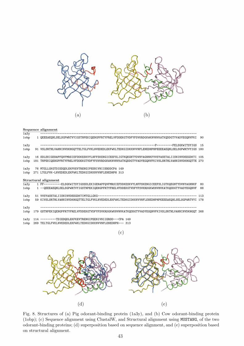
(a) (b)

Sequence alignment1a3y ------------------------------------------------------------------------------------------

1obp 1 QEEEAEQNLSELSGPWRTVYIGSTNPEKIQENGPFRTYFRELVFDDEKGTVDFYFSVKRDGKWKNVHVKATKQDDGTYVADYEGQNVFKI 90

1a3y ------------------------------------------------------------------P---------FELSGKWITSYIGS 15

1obp 91 VSLSRTHLVAHNINVDKHGQTTELTGLFVKLNVEDEDLEKFWKLTEDKGIDKKNVVNFLENEDHPHPEEEEAEQNLSELSGPWRTVYIGS 180

1a3y 16 SDLEKIGENAPFQVFMRSIEFDDKESKVYLNFFSKENGICEEFSLIGTKQEGNTYDVNYAGNNKFVVSYASETALIISNINVDEEGDKTI 105

1obp 181 TNPEKIQENGPFRTYFRELVFDDEKGTVDFYFSVKRDGKWKNVHVKATKQDDGTYVADYEGQNVFKIVSLSRTHLVAHNINVDKHGQTTE 270

1a3y 76 MTGLLGKGTDIEDQDLEKFKEVTRENGIPEENIVNIIERDDCPA 149

1obp 271 LTGLFVK-LNVEDEDLEKFWKLTEDKGIDKKNVVNFLENEDHPH 313

Structural alignment1a3y 1 PF----------ELSGKWITSYIGSSDLEKIGENAPFQVFMRSIEFDDKESKVYLNFFSKENGICEEFSLIGTKQEGNTYDVNYAGNNKF 80

1obp 1 --QEEEAEQNLSELSGPWRTVYIGSTNPEKIQENGPFRTYFRELVFDDEKGTVDFYFSVKRDGKWKNVHVKATKQDDGTYVADYEGQNVF 88

1a3y 51 VVSYASETALIISNINVDEEGDKTIMTGLLGKG--------------------------------------------------------- 113

1obp 59 KIVSLSRTHLVAHNINVDKHGQTTELTGLFVKLNVEDEDLEKFWKLTEDKGIDKKNVVNFLENEDHPHPEEEEAEQNLSELSGPWRTVYI 178

1a3y ------------------------------------------------------------------------------------------

1obp 179 GSTNPEKIQENGPFRTYFRELVFDDEKGTVDFYFSVKRDGKWKNVHVKATKQDDGTYVADYEGQNVFKIVSLSRTHLVAHNINVDKHGQT 268

1a3y 114 ---------TDIEDQDLEKFKEVTRENGIPEENIVNIIERDD---CPA 149

1obp 269 TELTGLFVKLNVEDEDLEKFWKLTEDKGIDKKNVVNFLENEDHPH--- 313

(c)

(d) (e)

Fig. 8. Structures of (a) Pig odorant-binding protein (1a3y), and (b) Cow odorant-binding protein(1obp); (c) Sequence alignment using ClustalW, and Structural alignment using MUSTANG, of the twoodorant-binding proteins; (d) superposition based on sequence alignment, and (e) superposition basedon structural alignment.

43

HOMSTRAD’s database alignment1cvl 121 DFVQDVLKTDPTGLSSTVIAAFVNVFGTLVSSSHNTDQDALAALRTLTTAQTATYNRNFP 1804lipd 120 DFVQGVLAYDPTGLSSTVIAAFVNVFGILTSSSNNTNQDALAALKTLTTAQAATYNQNYP 179MUSTANG’s alignment1cvl 121 DFVQDVLKTDPTGLS-STVIAAFVNVFGTLVSSS----HNTDQDALAALRTLTTAQTATY 1754lipd 120 DFVQGVLAYDPTGLSSTVIAAFVNVFGILTSSS-NNTNQ-DA---LAALKTLTTAQAATY 174

(a)

(b)

Fig. 9. (a) The region in the bacterial lipase family where the HOMSTRAD and MUSTANG alignmentsdisagree; (b) A visualisation of the region in the alignment showing the variability of the structureseven though the sequences in this region are almost identical. (1cvl–Yellow; 4lipd–Blue)

44

List of Tables

I Globin and Serine Proteinase data sets 46

II Results of comparisons on the globin data sets (see Table I) acrossthe multiple structural alignment programs MUSTANG, POSA, and CE-MC.(NCORE–The number of positions in the common core; RMSD–Averageroot-mean-square-deviation of the common core.) 47

III Results of comparisons on the globin data set described in Ochagavia andWodak [2004] across various programs. (NCORE–The number of positions inthe common core; RMSD–Average root-mean-square-deviation of the commoncore.) 48

IV Results of comparisons on the Serine proteinase data sets (Table I) acrossthe multiple structural alignment programs MUSTANG, POSA, and CE-MC.(NCORE–The number of positions in the common core; RMSD–Averageroot-mean-square-deviation of the common core.) 49

45

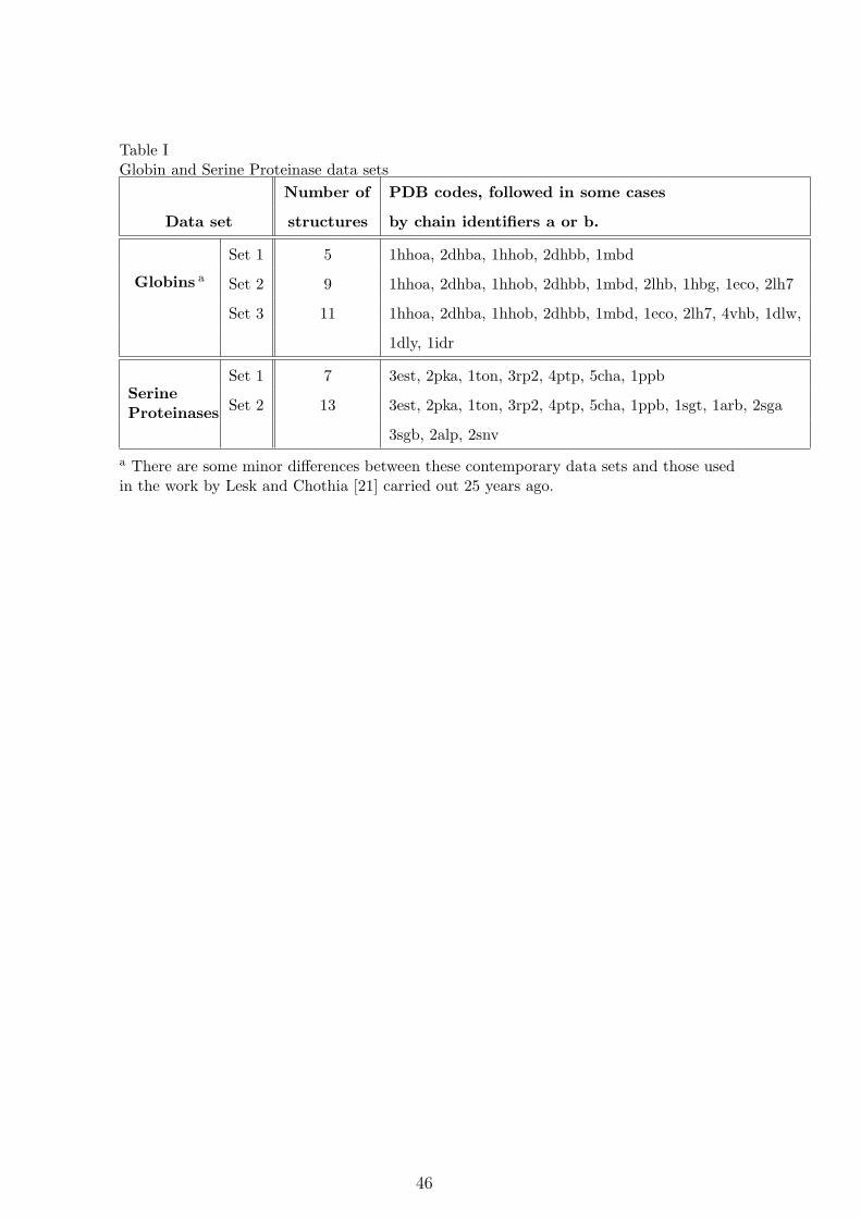
Table IGlobin and Serine Proteinase data sets

Number of PDB codes, followed in some cases

Data set structures by chain identifiers a or b.

Globins a

Set 1 5 1hhoa, 2dhba, 1hhob, 2dhbb, 1mbd

Set 2 9 1hhoa, 2dhba, 1hhob, 2dhbb, 1mbd, 2lhb, 1hbg, 1eco, 2lh7

Set 3 11 1hhoa, 2dhba, 1hhob, 2dhbb, 1mbd, 1eco, 2lh7, 4vhb, 1dlw,

1dly, 1idr

SerineProteinases

Set 1 7 3est, 2pka, 1ton, 3rp2, 4ptp, 5cha, 1ppb

Set 2 13 3est, 2pka, 1ton, 3rp2, 4ptp, 5cha, 1ppb, 1sgt, 1arb, 2sga

3sgb, 2alp, 2snv

a There are some minor differences between these contemporary data sets and those usedin the work by Lesk and Chothia [21] carried out 25 years ago.

46

Table IIResults of comparisons on the globin data sets (see Table I) across the multiple structural align-ment programs MUSTANG, POSA, and CE-MC. (NCORE–The number of positions in the common core;RMSD–Average root-mean-square-deviation of the common core.)

Globin MUSTANG POSA CE-MC

data Set NCORE RMSD NCORE RMSD NCORE RMSD

Set 1 139 1.41 A 139 1.47 A 138 1.40 A

Set 2 117 1.94 A 121 2.08 A 117 2.10 A

Set 3 94 2.24 A 90 2.32 A 92 2.47 A

47

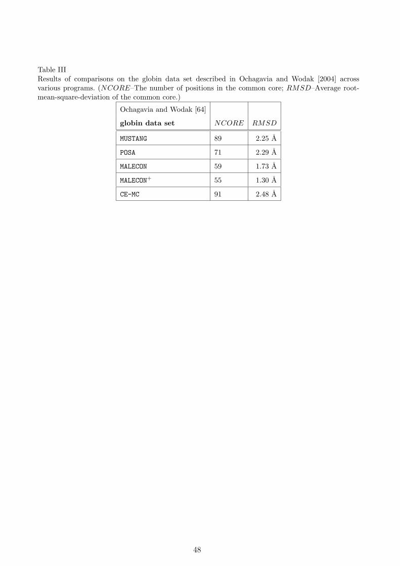
Table IIIResults of comparisons on the globin data set described in Ochagavia and Wodak [2004] acrossvarious programs. (NCORE–The number of positions in the common core; RMSD–Average root-mean-square-deviation of the common core.)

Ochagavia and Wodak [64]

globin data set NCORE RMSD

MUSTANG 89 2.25 A

POSA 71 2.29 A

MALECON 59 1.73 A

MALECON+ 55 1.30 A

CE-MC 91 2.48 A

48

Table IVResults of comparisons on the Serine proteinase data sets (Table I) across the multiple structuralalignment programs MUSTANG, POSA, and CE-MC. (NCORE–The number of positions in the commoncore; RMSD–Average root-mean-square-deviation of the common core.)

Serine Proteinase MUSTANG POSA CE-MC

data Set NCORE RMSD NCORE RMSD NCORE RMSD

Set 1 205 1.56 A 199 1.43 A – –

Set 2 119 2.42 A 86 2.00 A – –

49