MUSICAL INSTRUMENT SOURCESEPARATION IN UNISON AND

MONAURAL MIXTURES

a thesis

submitted to the department of computer engineering

and the graduate school of engineering and science

of bilkent university

in partial fulfillment of the requirements

for the degree of

master of science

By

Melik Berkan Ercan

August, 2014

I certify that I have read this thesis and that in my opinion it is fully adequate,

in scope and in quality, as a thesis for the degree of Master of Science.

Prof. Dr. H. Altay Guvenir (Advisor)

I certify that I have read this thesis and that in my opinion it is fully adequate,

in scope and in quality, as a thesis for the degree of Master of Science.

Prof. Dr. Bernd Edler (Co-Advisor)

I certify that I have read this thesis and that in my opinion it is fully adequate,

in scope and in quality, as a thesis for the degree of Master of Science.

Prof. Dr. A. Enis Cetin (Co-Advisor)

I certify that I have read this thesis and that in my opinion it is fully adequate,

in scope and in quality, as a thesis for the degree of Master of Science.

Assist. Prof. Dr. Oznur Tastan

I certify that I have read this thesis and that in my opinion it is fully adequate,

in scope and in quality, as a thesis for the degree of Master of Science.

Prof. Dr. Omer Morgul

Approved for the Graduate School of Engineering and Science:

Prof. Dr. Levent OnuralDirector of the Graduate School

ii

ABSTRACT

MUSICAL INSTRUMENT SOURCE SEPARATION INUNISON AND MONAURAL MIXTURES

Melik Berkan Ercan

M.S. in Computer Engineering

Supervisor: Prof. Dr. H. Altay Guvenir

August, 2014

Musical Instrument Source Separation aims to separate the individual instru-

ments from a mixture. We work on mixtures where there are two instruments,

playing the same constant pitch at the same time. When musical instruments play

the same note, they overlap with each other and act as a single source. We use

statistical source separation algorithms which perform separation by maximizing

the statistical independence between the sources. A mixture can be recorded with

more than one microphone; this enables us to extract spatial information of the

instruments by comparing the recordings. However we work with the monaural

case where there is one microphone. Some musical instruments have amplitude

modulation and this modulation can be seen in the mixtures. We also aim to

detect amplitude modulations to support the source separation success. We use

NTF (Non-negative tensor factorization) to perform the separation. NTF sepa-

rates the mixture into many components. These components should be clustered

in order to synthesize the individual sources. We use k-means as well as man-

ual clustering by comparing the SDR (Signal to Distortion Ratio) values of the

components with the original sources.

Keywords: Source Separation, Statistical Source Separation, Monaural, Unison

mixture, NMF, NTF.

iii

OZET

UNISON VE MONAURAL MUZIK ENSTRUMANIKARISIMLARINDA KAYNAK AYIRMA

Melik Berkan Ercan

Bilgisayar Muhendisligi, Yuksek Lisans

Tez Yoneticisi: Prof. Dr. H. Altay Guvenir

Agustos, 2014

Muzik Enstrumanlarında kaynak ayırma islemi, bir ses karısımı icindeki ses-

leri ayırmayı hedefler. Bu calısmada, aynı anda, aynı sabit notayı calan, iki

enstrumandan olusan karısımlar uzerinde calısılmıstır. Muzik Enstrumanları

aynı notayı caldıgında olusan sesler, birbirleri icinde karısıp tek bir sesmis

gibi algılanırlar. Bu calısmada, bu sesleri ayırmak icin istatistiksel kaynak

ayırma algoritmaları kullanılmıstır. Bu algoritmalar sesler arasındaki istatistik-

sel bagımlılıgı maksimum yapmaya calısarak ses ayırma islemini gerceklestirirler.

Bir karısım birden cok mikrofon kullanılarak kayıt edilebilir; bu durum kayıtları

birbiriyle karsılastırarak enstrumanlarla ilgili konum bilgisinin cıkarılmasını

saglar. Burada tek mikrofon ile alınmıs kayıtlar kullanılmıstır. Bazı muzik en-

strumanlarında genlik modulasyonu vardır ve bu modulasyon bir karısım icinde

de gozlemlenebilir. Bu calısmada, genlik modulasyonu tespit edilerek kaynak

ayırma kalitesi arttırılmaya calısılmıstır. Kaynak ayırma islemi icin NTF (Non-

negative Tensor Factorization) algoritması kullanılmıstır. NTF, karısımı birden

cok bilesene ayırır. Kaynak sesleri tekrar elde etmek icin bu bilesenlerin uygun bir

sekilde birlestirilmesi gerekir. Bu birlestirme islemi icin ise k-means demetleme al-

gorithması ve bunun yanında el ile birlestirme yapılmıstır. El ile birlestirme islemi

icin bilesenlerin SDR (Signal to Distortion Ratio) degerleri orjinal kaynaklar ile

karsılastırılmıstır.

Anahtar sozcukler : Kaynak Ayırma, Istatistiksel Kaynak Ayırma, Unison

Karısım, Monaural, NMF, NTF.

iv

Acknowledgement

I would like to express my gratitude to my supervisors Prof. Dr. Altay Guvenir,

Prof. Dr. Bernd Edler and Martina Spengler for the opportunity to work on

my thesis in Fraunhofer IIS Audiolabs in cooperation with Bilkent University. I

also want to thank Fabian Robert Stoter for introducing me to the topic, for his

supervision and for his countless days of effort for our research. Furthermore I

want to thank Esther, Maja, Maneesh, Orcun and Vivi for their friendship and

support.

Last but not least, I want to thank my family; Filiz, Ismail and Berkin for their

support.

v

Contents

1 Introduction 1

2 Background 5

2.1 Amplitude and Frequency Modulation . . . . . . . . . . . . . . . 8

2.2 Musical Instruments . . . . . . . . . . . . . . . . . . . . . . . . . 10

2.3 Terminology . . . . . . . . . . . . . . . . . . . . . . . . . . . . . . 12

3 Related Work 15

3.1 Independent Component Analysis (ICA) . . . . . . . . . . . . . . 16

3.2 Independent Subspace Analysis (ISA) . . . . . . . . . . . . . . . . 18

3.3 Non-Negative Matrix Factorization (NMF) . . . . . . . . . . . . . 19

3.4 Non-Negative Tensor Factorization (NTF) . . . . . . . . . . . . . 21

3.5 Computational Auditory Scene Analysis (CASA) . . . . . . . . . 22

4 The NTF Based Source Separation Algorithm 24

4.1 The NTF Based Algorithm . . . . . . . . . . . . . . . . . . . . . . 25

vi

CONTENTS vii

4.1.1 DFT Filterbank . . . . . . . . . . . . . . . . . . . . . . . . 25

4.1.2 Tensor Representation . . . . . . . . . . . . . . . . . . . . 28

4.1.3 The NTF algorithm . . . . . . . . . . . . . . . . . . . . . . 29

4.1.4 Reconstruction . . . . . . . . . . . . . . . . . . . . . . . . 33

4.1.5 Clustering . . . . . . . . . . . . . . . . . . . . . . . . . . . 36

4.2 The Test Data . . . . . . . . . . . . . . . . . . . . . . . . . . . . . 38

4.3 Experiment and Results . . . . . . . . . . . . . . . . . . . . . . . 45

4.3.1 Performance Evaluation . . . . . . . . . . . . . . . . . . . 45

4.3.2 Discussion . . . . . . . . . . . . . . . . . . . . . . . . . . . 48

5 Conclusion 50

List of Figures

2.1 Different domain representations . . . . . . . . . . . . . . . . . . . 6

2.2 Two sine wave with different frequencies added . . . . . . . . . . 7

2.3 Amplitude modulation visualization . . . . . . . . . . . . . . . . . 9

2.4 Frequency modulation visualization . . . . . . . . . . . . . . . . . 10

2.5 A cello signal in three different domain representations . . . . . . 11

2.6 Spectrograms of four different signals . . . . . . . . . . . . . . . . 12

3.1 Cocktail party problem1 . . . . . . . . . . . . . . . . . . . . . . . 17

4.1 The NTF based separation algorithm pipeline . . . . . . . . . . . 26

4.2 DFT filterbank bins . . . . . . . . . . . . . . . . . . . . . . . . . . 27

4.3 NTF decomposition of a single sine wave . . . . . . . . . . . . . . 28

4.4 Tensor decomposition for the mixture of two sine waves . . . . . . 29

4.5 Tensor decomposition for the mixture of two sine waves with AM 30

4.6 Tensor decomposition for piano and cello mixture . . . . . . . . . 31

4.7 The separation result when k = 6 . . . . . . . . . . . . . . . . . . 32

viii

LIST OF FIGURES ix

4.8 Tensor decomposition for piano and cello mixture with 4 components 33

4.9 2-Step NTF pipeline . . . . . . . . . . . . . . . . . . . . . . . . . 34

4.10 The NMF based separation algorithm pipeline for k = 6 . . . . . . 35

4.11 Various single sine waves . . . . . . . . . . . . . . . . . . . . . . . 37

4.12 Various signals with two sine waves . . . . . . . . . . . . . . . . . 38

4.13 Signals with modulation effects and different start times . . . . . 39

4.14 Singals with harmonics . . . . . . . . . . . . . . . . . . . . . . . 40

4.15 Spectrograms of test files . . . . . . . . . . . . . . . . . . . . . . . 41

4.16 Piano and cello mixture . . . . . . . . . . . . . . . . . . . . . . . 42

4.17 Flute and horn mixture . . . . . . . . . . . . . . . . . . . . . . . . 43

4.18 Oboe and violin mixture . . . . . . . . . . . . . . . . . . . . . . . 44

4.19 Listening test instrument comparison . . . . . . . . . . . . . . . . 46

4.20 Listening test algorithm comparison . . . . . . . . . . . . . . . . . 47

4.21 Clustering results for piano and cello mixture . . . . . . . . . . . 48

4.22 Clustering results for oboe and bassoon mixture . . . . . . . . . . 49

Chapter 1

Introduction

Almost all of the sounds we hear in our daily life are combination of many in-

dividual sounds. Examples could be a conversation, a song, singing birds or a

car traffic. Those sound sources are formed by a combination of simpler tones

and more than one sound may exist in the same medium at the same time. In

such an environment, a listener would likely to be interested in a single source

among the existing sounds. Thus, the listener faces the task to separate or ex-

tract the source of interest among the mixture. The cognitive ability of human

auditory system enables us to follow a speaker in a noisy environment. This

ability makes use of similar techniques with source separation algorithms. Thus

source separation is a concept that we are not completely unfamiliar with. A

formal definition of a source separation task would be to identify and separate

the different sound sources in a sound mixture. Even though this task is natural

and easy for humans, it is challenging to develop an algorithm that performs the

same task, automatically.

When two sound sources travel through the same medium, the mixture is the

superposition of the sinusoidal components [1]. The similarity of the sources

affects how the sources are superposed. When two signals are similar, they will

share some of their frequency components. The more similar two sound sources

are, the more frequency components they will share. So the original information of

the individual sources will not be preserved in the mixture as they are superposed.

1

As a result, working with the mixture of similar sound files are difficult. It is

important to come up with a similarity definition. In this thesis, the similarity of

two signals is evaluated by the correlation of their frequency spectrum. In other

words, the comparison of the common frequency components of two signals is a

measurement method of similarity.

Working with musical instrument mixtures are similar to working with daily

sound sources. However, when a group of instruments play together, they play

in harmony; in order to create a common sound that would please the audience.

This means they will be playing the same note or harmonic notes at the same

time, which further means the individual instruments will share their frequencies.

This source separation task is harder, since the instruments will be mixed with

each other. Conversely in a speech file, even though two speakers are speaking

at the same time, it would be unlikely for them to generate the same pitches. In

a typical case with two speakers, only one speaker will speak at a time. Thus

source separation in speech files is relatively simpler.

When two instruments play the same tone, or the same note on a different oc-

tave, it is called a unison sound [2]. In this thesis, we work on the unison source

separation problem where two musical instruments are playing at the same pitch.

Since the sources have the same pitch, the spectral similarity of the sources is

expected to be high; almost all the frequency components exist in both sources.

In addition to that, we work with single channel recordings. These recordings are

captured by using a single microphone and called monaural. The recordings that

captured with more than one microphone are called multi-channel recordings. A

multiple channel recording captures the mixture sound from different locations.

This means by using multi-channel recording, we can capture the spatial infor-

mation of the sources. There are some source separation algorithms such as ICA

[3], which uses this spatial location information to separate sources. In summary,

we say that we work with monaural unison mixtures.

A source separation system can have many different application areas. As men-

tioned earlier, source separation algorithms can be applied to both music and

speech signals. In music, extraction or separation of the instruments can be used

2

for instrumental training; musicians can play along with the mixture with one or

more of the instruments removed. Musicians would also be interested in listening

to an instrument individually. Source separation can also be used for recovering

an old record from noise artifacts. Most of the old vinyl recordings have noise

artifacts or distorted areas. Reconstruction of those areas is an important ap-

plication scenario. Speech audio has a wider range of application topics; but in

general, the main aim of source separation is to attenuate all the sources other

than the desired source. Perhaps the most famous source separation problem is

known as the Cocktail Party Problem [4]. This task is to capture a speaker’s

voice in a noisy environment where there exists many sound sources, generating

sound at the same time.

Any prior information about the source separation problem scenario is useful

since it can help to define the problem scenario better and might give hints about

the sources. Those hints can be given within the problem domain or can be

retrieved through pre-processing of the input data [5]. For the musical instrument

separation case, this information includes, number of instruments, instrument

types, playing style, sheet music, mixing methodology, recording environment,

etc. For the speech separation case, this information can be, number of speakers,

gender of the speakers, recording environment, etc. However in some source

separation tasks, no prior information is available. In this case the separation

task is called blind or unsupervised source separation. Any source separation

task with any prior information is called supervised source separation. Note that

our system performs blind source separation.

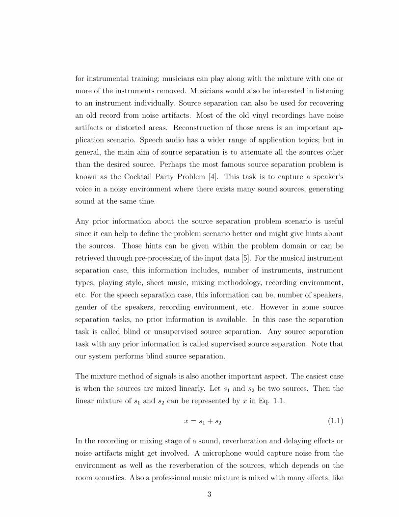
The mixture method of signals is also another important aspect. The easiest case

is when the sources are mixed linearly. Let s1 and s2 be two sources. Then the

linear mixture of s1 and s2 can be represented by x in Eq. 1.1.

x = s1 + s2 (1.1)

In the recording or mixing stage of a sound, reverberation and delaying effects or

noise artifacts might get involved. A microphone would capture noise from the

environment as well as the reverberation of the sources, which depends on the

room acoustics. Also a professional music mixture is mixed with many effects, like

3

distortion, modulation, reverberation, delay, etc. These effects create mixtures

that are hard to work on. Therefore, we work with linear mixed signals and we do

not work with songs. We have generated various individual musical instrument

files and we mix them linearly as shown in Eq. 1.1.

Second chapter gives background information about the source separation task

and introduces some of the popular blind source separation algorithms. The

third chapter introduces the related work. The Fourth Chapter proposes the

NTF based algorithm that is specifically designed for monaural and unison mix-

tures. We also introduce the test set, various implementations of our NTF based

algorithm and the test scenarios that we have tried our algorithm on. The final

chapter is conclusion where all the work is summarized. Conclusion chapter also

covers the potential future work.

4

Chapter 2

Background

In this chapter, we provide background information about the thesis topics in

order to give a basic understanding of the source separation algorithms and pro-

cedures that we employ. Some background information on signals and systems

and Digital Signal Processing should be given. The concepts that we have used

in the thesis will be explained. This chapter should be enough to understand the

main work that we have done. The basic properties of sine waves and how to com-

bine them will be given in order to understand musical instruments. Amplitude

and frequency modulation concepts will also be introduced. They are widely used

for communication purposes. In addition, we have the background information of

signal processing by explaining various fourier transformation implementations,

zero padding, windowing, filters, filterbanks, sampling frequency, etc.

A sound signal is a pattern of variation which is used to carry or represent in-

formation [6]. A sound signal can be a pure tone or a complex tone, which can

be thought as the mixture of pure tones. A pure tone is a sound signal which is

formed by a single sine wave. The mathematical explanation of a sine wave is as

follows;

x(t) = A · sin(w0t+ φ) (2.1)

where w0 = 2πf and A, f , w0, φ are amplitude, frequency, radiant frequency and

phase shift respectively. In this thesis, we work both with sinusoidal signals and

5

0 2 4 6 8 10 12 14 16 18 20

−0.2

−0.1

0

0.1

0.2

time (msec)

Am

plit

ude

a) Time Domain

0 200 400 600 800 1000 1200 1400 16000

2

4

6

8

10x 10

4

frequency (Hz)

Magnitude

b) Frequency Domain

Figure 2.1: Different domain representations

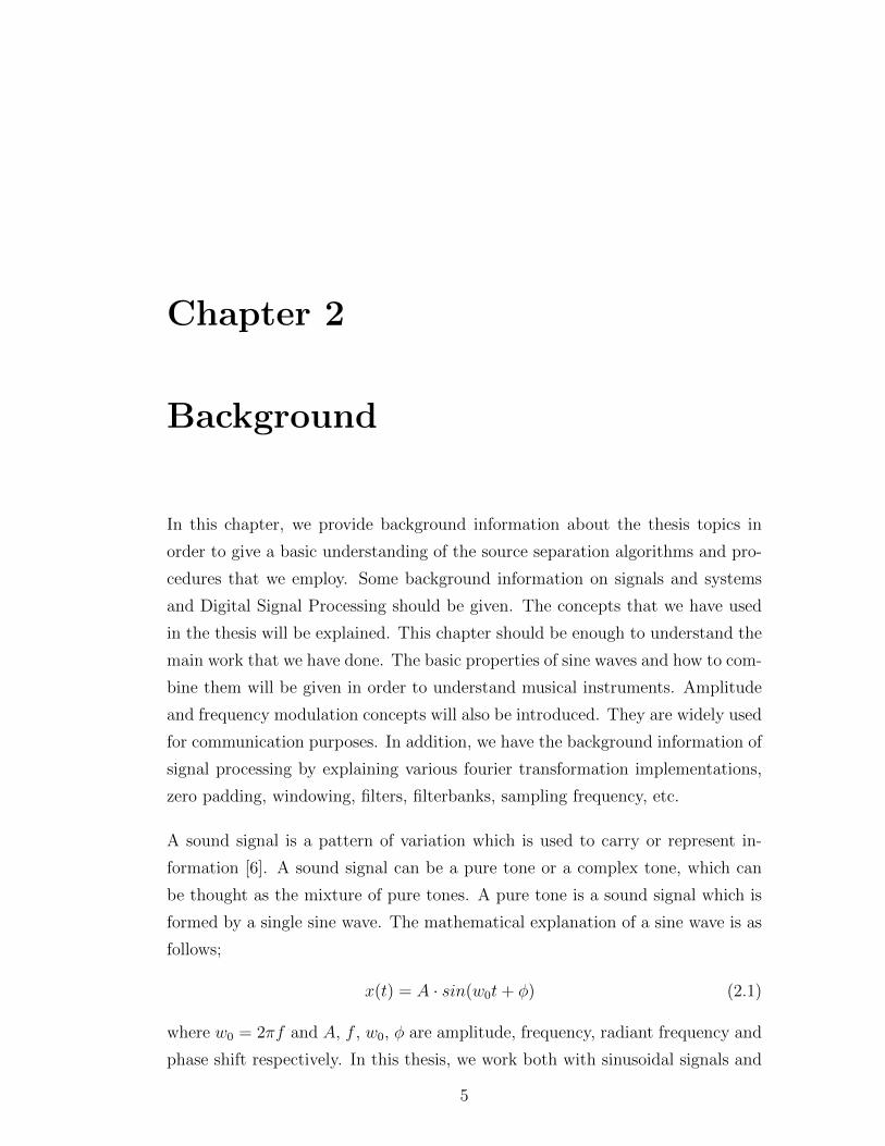
complex signals. From the mathematical expression of a sine wave, we see that

a sine wave takes values between −A and A with respect to time and frequency.

Figure 2.1a is the visualization of a sine wave with A = 0.25, f = 440 Hz and

zero phase. It can be represented with the following formula; x1(t) = 0.25 ·sin(2π440t + 0). This representation of the sinusoidal signal is in time domain

and in this domain, we have the information of the amplitude of the sine wave with

respect to time. Time domain information alone is often not enough to process or

learn about the signal. We can also switch to the frequency domain by applying

Fourier transformation. This transformation is performed by an algorithm called

Discrete Frequency Transformation (DFT). We will not go through the details of

DFT, since there is a practical implementation of it, which is called Fast Fourier

Transformation (FFT). For more information, please refer to this resource [6,

p.402]. The frequency domain representation of a signal shows which frequencies

6

0 2 4 6 8 10 12 14 16 18 20

−0.3

−0.2

−0.1

0

0.1

0.2

0.3

time (msec)

Am

plit

ude

a) Time Domain

0 200 400 600 800 1000 1200 1400 16000

2

4

6

8

10x 10

4

frequency (Hz)

Magnitude

b) Frequency Domain

Figure 2.2: Two sine wave with different frequencies added

are included in the signal. Figure 2.1b shows the frequency representation of

x1(t). Since x1(t) consists of a single sine wave with frequency 440 Hz, there is a

single peak in the figure 2.1b.

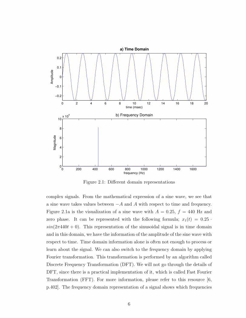
Let x2(t) denote another sine wave with the following properties. A = 0.25,

f = 440 × 3 = 1320 Hz and zero phase. It can also be represented with the

following formula. x2(t) = 0.25 · sin(2π1320t + 0). Figure 2.2 shows the linear

addition of x1(t) and x2(t). The superposed sine waves are shown in time and

frequency domain in Figure 2.2a and 2.2b respectively.

7

2.1 Amplitude and Frequency Modulation

Some musical instruments have amplitude modulation or frequency modulation.

Our aim is to be able to detect that modulation and use it to separate instru-

ments with modulation. Therefore we first need to know how amplitude modu-

lation looks like in time and frequency domain. Amplitude modulation is used

in communication to carry information through a signal which has relatively low

frequency, when compared to the carrier. This increases the message range. To

learn more about the amplitude and frequency modulation for communication

purposes, the reader is referred to the book by Godse and Bakshi (2009) [7].

Other than communication purposes, some of the musical instruments also have

amplitude and frequency modulation. It exists because of the physical nature

of the instrument or it might be because of the playing style of the instrument.

For example, a piano does not have amplitude or frequency modulation whereas

a violin have amplitude and frequency modulation both from the playing style

and the physical nature of the instrument. Detection of amplitude and frequency

modulation in an instrument signal is not a hard, but rather a complicated task

[8]. Even though we worked on the detection of modulation effects in musical

instruments, we will not go into details since it is not in the context of the thesis.

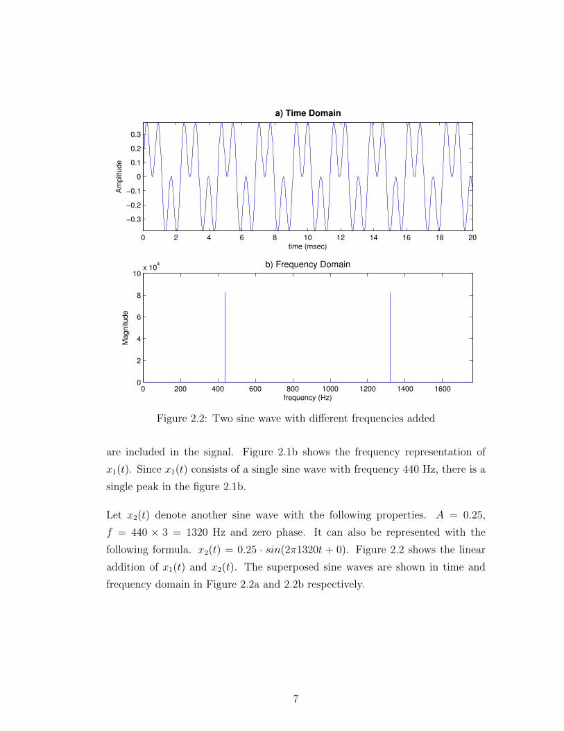
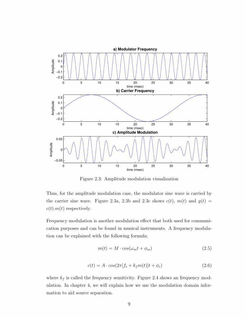
The simple theory and the mathematical representation of amplitude modulation

is as follows; a sine wave at certain frequency f0 can be modulated by another

sinusoid with frequency f1 when they pass through the same medium and if

f0 >> f1. The sine wave with the frequency f1 is called the carrier and denoted

by c(t). The other sine wave with the frequency f0 is called the modulator and

denoted by m(t). We denote their superposition with y(t).

c(t) = A · cos(ωct+ φc) (2.2)

m(t) = M · cos(ωmt+ φm) (2.3)

y(t) = c(t).m(t) (2.4)

8

0 5 10 15 20 25 30 35 40

−0.2

−0.1

0

0.1

0.2

time (msec)

Am

plit

ude

a) Modulator Frequency

0 5 10 15 20 25 30 35 40

−0.2

−0.1

0

0.1

0.2

time (msec)

Am

plit

ude

b) Carrier Frequency

0 5 10 15 20 25 30 35 40

−0.05

0

0.05

time (msec)

Am

plit

ude

c) Amplitude Modulation

Figure 2.3: Amplitude modulation visualization

Thus, for the amplitude modulation case, the modulator sine wave is carried by

the carrier sine wave. Figure 2.3a, 2.3b and 2.3c shows c(t), m(t) and y(t) =

c(t).m(t) respectively.

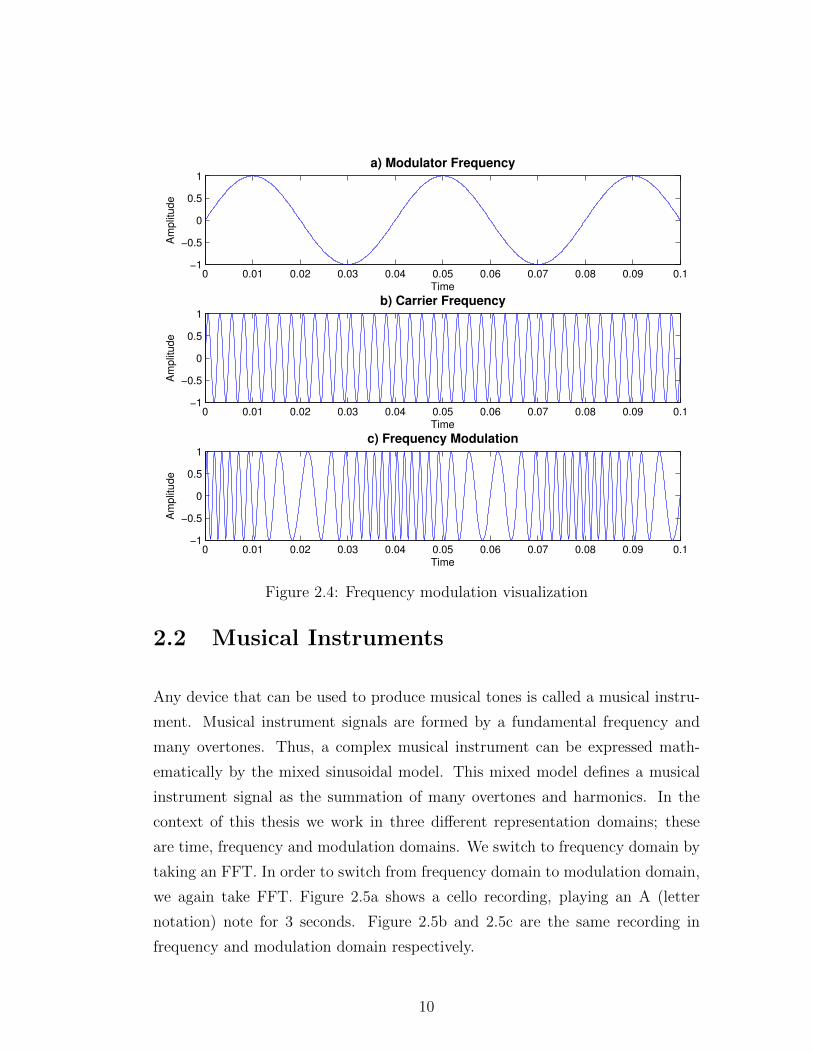
Frequency modulation is another modulation effect that both used for communi-

cation purposes and can be found in musical instruments. A frequency modula-

tion can be explained with the following formula;

m(t) = M · cos(ωmt+ φm) (2.5)

c(t) = A · cos(2π[fc + kfm(t)]t+ φc) (2.6)

where kf is called the frequency sensitivity. Figure 2.4 shows an frequency mod-

ulation. In chapter 4, we will explain how we use the modulation domain infor-

mation to aid source separation.

9

0 0.01 0.02 0.03 0.04 0.05 0.06 0.07 0.08 0.09 0.1−1

−0.5

0

0.5

1

Time

Am

plit

ude

a) Modulator Frequency

0 0.01 0.02 0.03 0.04 0.05 0.06 0.07 0.08 0.09 0.1−1

−0.5

0

0.5

1

Time

Am

plit

ude

b) Carrier Frequency

0 0.01 0.02 0.03 0.04 0.05 0.06 0.07 0.08 0.09 0.1−1

−0.5

0

0.5

1

Time

Am

plit

ude

c) Frequency Modulation

Figure 2.4: Frequency modulation visualization

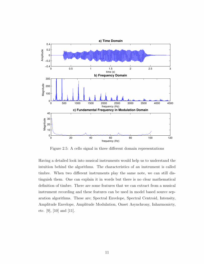
2.2 Musical Instruments

Any device that can be used to produce musical tones is called a musical instru-

ment. Musical instrument signals are formed by a fundamental frequency and

many overtones. Thus, a complex musical instrument can be expressed math-

ematically by the mixed sinusoidal model. This mixed model defines a musical

instrument signal as the summation of many overtones and harmonics. In the

context of this thesis we work in three different representation domains; these

are time, frequency and modulation domains. We switch to frequency domain by

taking an FFT. In order to switch from frequency domain to modulation domain,

we again take FFT. Figure 2.5a shows a cello recording, playing an A (letter

notation) note for 3 seconds. Figure 2.5b and 2.5c are the same recording in

frequency and modulation domain respectively.

10

0 0.5 1 1.5 2 2.5 3−0.4

−0.2

0

0.2

0.4

time (s)

Am

plit

ude

a) Time Domain

0 500 1000 1500 2000 2500 3000 3500 4000 45000

100

200

300

frequency (Hz)

Magnitude

b) Frequency Domain

0 20 40 60 80 100 1200

10

20

30

40

frequency (Hz)

Magnitude

c) Fundamental Frequency in Modulation Domain

Figure 2.5: A cello signal in three different domain representations

Having a detailed look into musical instruments would help us to understand the

intuition behind the algorithms. The characteristics of an instrument is called

timbre. When two different instruments play the same note, we can still dis-

tinguish them. One can explain it in words but there is no clear mathematical

definition of timbre. There are some features that we can extract from a musical

instrument recording and these features can be used in model based source sep-

aration algorithms. These are; Spectral Envelope, Spectral Centroid, Intensity,

Amplitude Envelope, Amplitude Modulation, Onset Asynchrony, Inharmonicty,

etc. [9], [10] and [11].

11

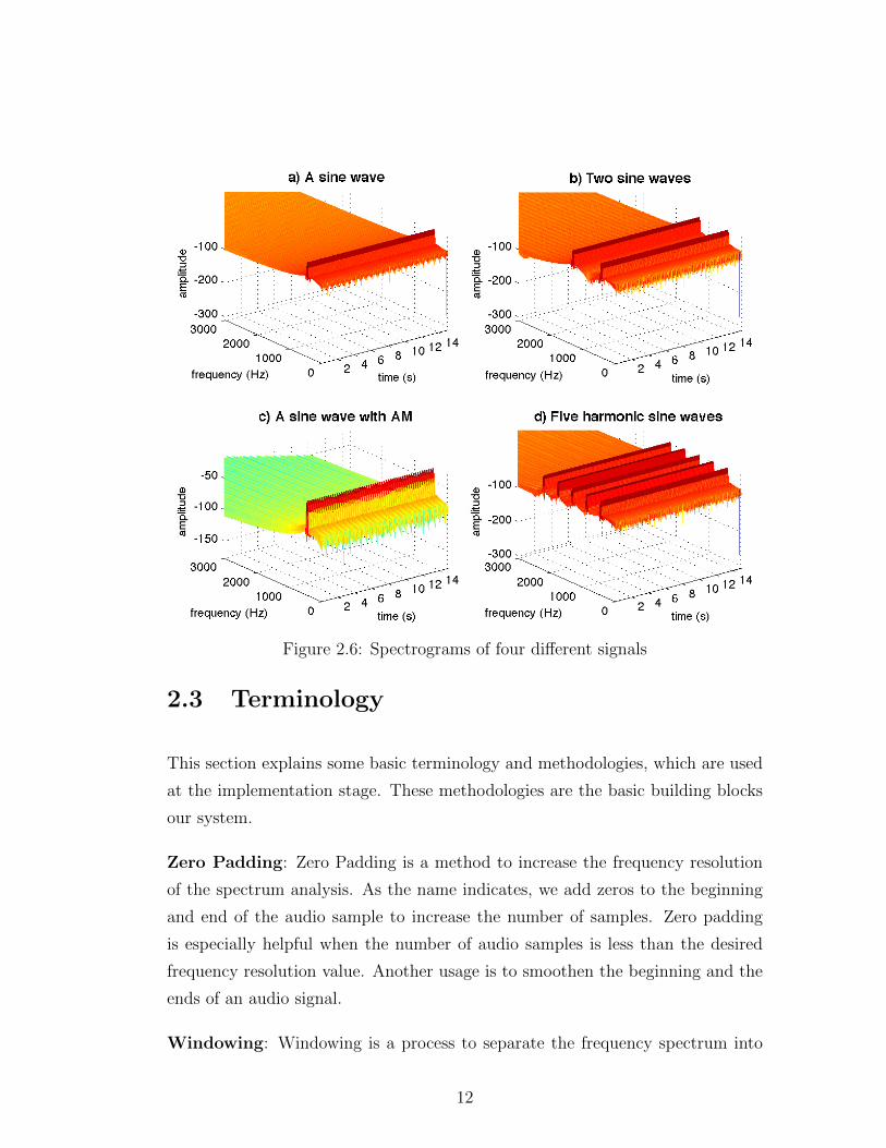
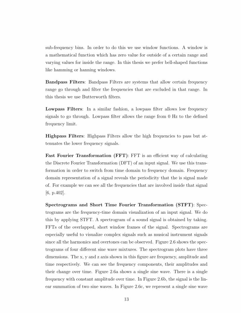
Figure 2.6: Spectrograms of four different signals

2.3 Terminology

This section explains some basic terminology and methodologies, which are used

at the implementation stage. These methodologies are the basic building blocks

our system.

Zero Padding: Zero Padding is a method to increase the frequency resolution

of the spectrum analysis. As the name indicates, we add zeros to the beginning

and end of the audio sample to increase the number of samples. Zero padding

is especially helpful when the number of audio samples is less than the desired

frequency resolution value. Another usage is to smoothen the beginning and the

ends of an audio signal.

Windowing: Windowing is a process to separate the frequency spectrum into

12

sub-frequency bins. In order to do this we use window functions. A window is

a mathematical function which has zero value for outside of a certain range and

varying values for inside the range. In this thesis we prefer bell-shaped functions

like hamming or hanning windows.

Bandpass Filters: Bandpass Filters are systems that allow certain frequency

range go through and filter the frequencies that are excluded in that range. In

this thesis we use Butterworth filters.

Lowpass Filters: In a similar fashion, a lowpass filter allows low frequency

signals to go through. Lowpass filter allows the range from 0 Hz to the defined

frequency limit.

Highpass Filters: Highpass Filters allow the high frequencies to pass but at-

tenuates the lower frequency signals.

Fast Fourier Transformation (FFT): FFT is an efficient way of calculating

the Discrete Fourier Transformation (DFT) of an input signal. We use this trans-

formation in order to switch from time domain to frequency domain. Frequency

domain representation of a signal reveals the periodicity that the is signal made

of. For example we can see all the frequencies that are involved inside that signal

[6, p.402].

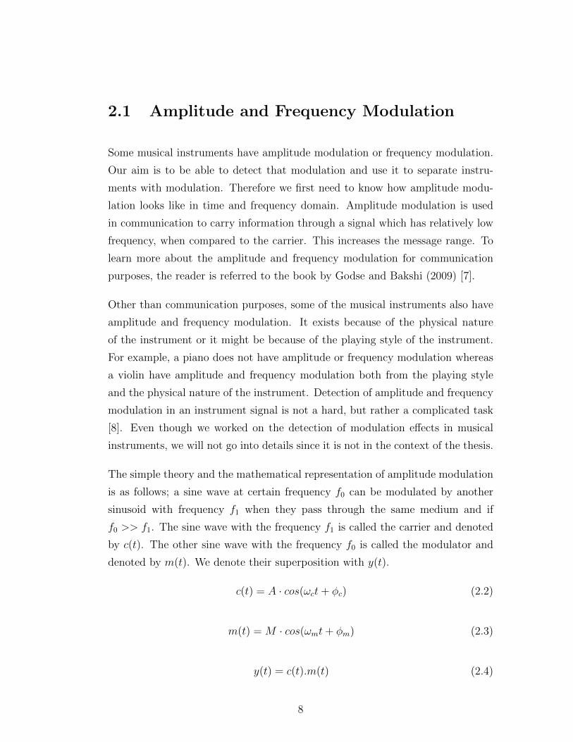
Spectrograms and Short Time Fourier Transformation (STFT): Spec-

trograms are the frequency-time domain visualization of an input signal. We do

this by applying STFT. A spectrogram of a sound signal is obtained by taking.

FFTs of the overlapped, short window frames of the signal. Spectrograms are

especially useful to visualize complex signals such as musical instrument signals

since all the harmonics and overtones can be observed. Figure 2.6 shows the spec-

trograms of four different sine wave mixtures. The spectrogram plots have three

dimensions. The x, y and z axis shown in this figure are frequency, amplitude and

time respectively. We can see the frequency components, their amplitudes and

their change over time. Figure 2.6a shows a single sine wave. There is a single

frequency with constant amplitude over time. In Figure 2.6b, the signal is the lin-

ear summation of two sine waves. In Figure 2.6c, we represent a single sine wave

13

with modulation frequency. The amplitude is fluctuating over time. Finally, the

signal in Figure 2.6d has five peaks since that signal is formed by linearly adding

five sine wave. As you notice we can gather many information about the signal

from spectrograms. Another advantage of spectrogram is it’s data representation.

We represent a spectrogram in a 2D matrix where each row is a frequency range,

namely filter bins. Most of the signal processing tasks require us to work on

frequency bins separately. Therefore we can use the spectrogram representation

to divide the signal into frequency bins, process specific bins [6, p.408].

Filterbanks: Filterbanks are formed of band-pass filters that are used to sepa-

rate the input into many frequency bins. We use filterbanks due to their represen-

tation capabilities. The spectrogram representation we explained earlier is also

in this category. When the parameters are correctly chosen, the filterbank repre-

sentation can put all the frequencies into separate frequency bins. A gammatone

filterbank is designed to separate a signal into frequency bins according to the

human auditory system. The cochlea in the human auditory system separates the

frequencies non-linearly. Thus gammatone filterbank mimics the functionality of

cochlea. This is very useful for the applications that are related with human

hearing, sound perception, etc. DFT filterbank is identical with the spectrogram

representation. It is to separate the frequency bins with same interval range.

14

Chapter 3

Related Work

This chapter covers existing source separation algorithms that are proposed for

the Blind Source Separation problem. These algorithms help us to understand

the fundamental approaches as well as the nature of the musical instrument sound

sources. Furthermore, the intuition behind existing algorithms reveals a better

understanding about the problem domain. It might also help us to propose new

problem solving methodologies in the future, by observing the strong and the

weak points of the existing algorithms. The algorithms that we are going to in-

troduce can be divided into two main categories; the first category is unsupervised

source separation algorithms. The algorithms in this category follow information-

theoretical principals such as statistical independence [12]. The second category

contains supervised algorithms. These algorithms use prior information about

the system to learn a model. These algorithms use the classical machine learn-

ing approaches to learn a model [13]. There are also algorithms which model

the human auditory system to mimic the human segregation capabilities. As ex-

plained earlier, human auditory system processes the sounds in a way that the

same techniques can be used to perform source separation.

The unsupervised learning methods that we are going to explain use the linear

signal model. The linear signal model assumes that, when two sound sources

are present in the same environment, the waveform of the mixture is the linear

summation of the sources [14].

15

3.1 Independent Component Analysis (ICA)

ICA is one of the successful algorithms that can be used in blind source separa-

tion task. The strategy behind ICA is to decompose the mixture into components

that are as statistically independent as possible. In mathematics, statistical in-

dependence of two variables is defined as follows; random variables x and y are

said to be independent if their joint probability distribution function p(x, y) is a

product of the marginal distribution functions, p(x, y) = p(x)p(y) [15]. Statistical

dependence can also be defined as the mutual information between two source.

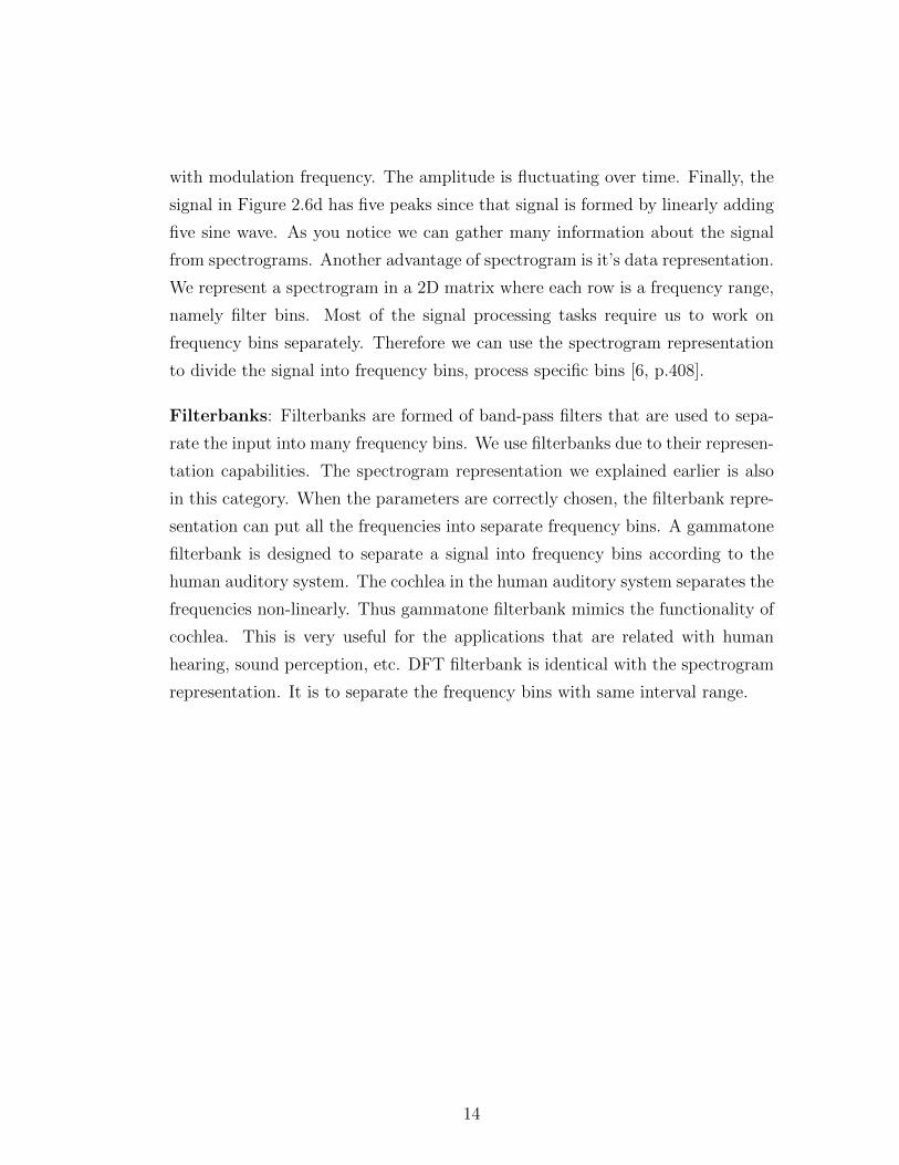
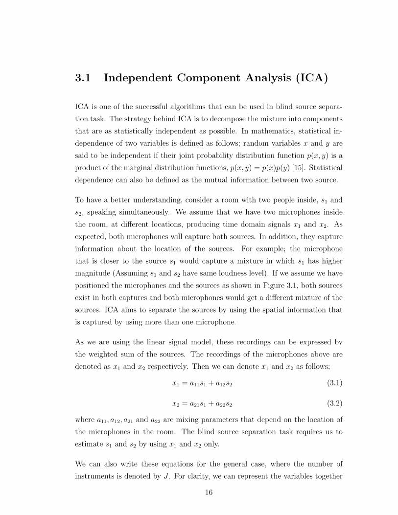
To have a better understanding, consider a room with two people inside, s1 and

s2, speaking simultaneously. We assume that we have two microphones inside

the room, at different locations, producing time domain signals x1 and x2. As

expected, both microphones will capture both sources. In addition, they capture

information about the location of the sources. For example; the microphone

that is closer to the source s1 would capture a mixture in which s1 has higher

magnitude (Assuming s1 and s2 have same loudness level). If we assume we have

positioned the microphones and the sources as shown in Figure 3.1, both sources

exist in both captures and both microphones would get a different mixture of the

sources. ICA aims to separate the sources by using the spatial information that

is captured by using more than one microphone.

As we are using the linear signal model, these recordings can be expressed by

the weighted sum of the sources. The recordings of the microphones above are

denoted as x1 and x2 respectively. Then we can denote x1 and x2 as follows;

x1 = a11s1 + a12s2 (3.1)

x2 = a21s1 + a22s2 (3.2)

where a11, a12, a21 and a22 are mixing parameters that depend on the location of

the microphones in the room. The blind source separation task requires us to

estimate s1 and s2 by using x1 and x2 only.

We can also write these equations for the general case, where the number of

instruments is denoted by J . For clarity, we can represent the variables together

16

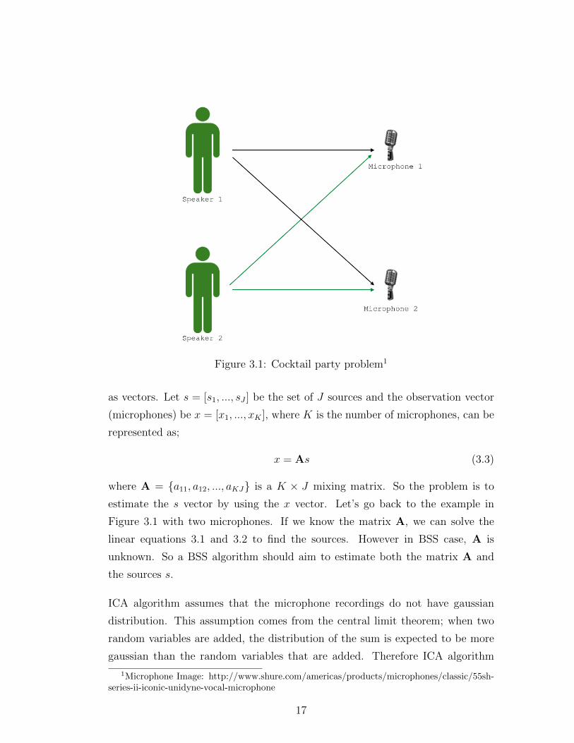
Figure 3.1: Cocktail party problem1

as vectors. Let s = [s1, ..., sJ ] be the set of J sources and the observation vector

(microphones) be x = [x1, ..., xK ], where K is the number of microphones, can be

represented as;

x = As (3.3)

where A = {a11, a12, ..., aKJ} is a K × J mixing matrix. So the problem is to

estimate the s vector by using the x vector. Let’s go back to the example in

Figure 3.1 with two microphones. If we know the matrix A, we can solve the

linear equations 3.1 and 3.2 to find the sources. However in BSS case, A is

unknown. So a BSS algorithm should aim to estimate both the matrix A and

the sources s.

ICA algorithm assumes that the microphone recordings do not have gaussian

distribution. This assumption comes from the central limit theorem; when two

random variables are added, the distribution of the sum is expected to be more

gaussian than the random variables that are added. Therefore ICA algorithm

1Microphone Image: http://www.shure.com/americas/products/microphones/classic/55sh-series-ii-iconic-unidyne-vocal-microphone

17

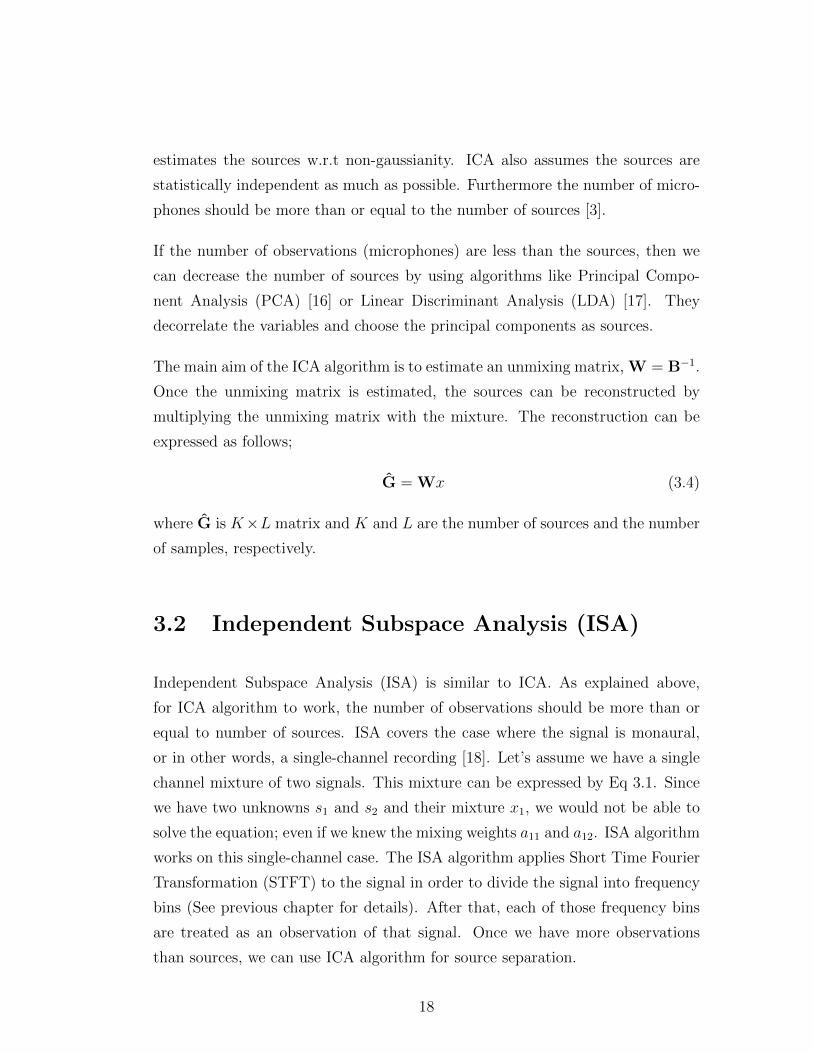
estimates the sources w.r.t non-gaussianity. ICA also assumes the sources are

statistically independent as much as possible. Furthermore the number of micro-

phones should be more than or equal to the number of sources [3].

If the number of observations (microphones) are less than the sources, then we

can decrease the number of sources by using algorithms like Principal Compo-

nent Analysis (PCA) [16] or Linear Discriminant Analysis (LDA) [17]. They

decorrelate the variables and choose the principal components as sources.

The main aim of the ICA algorithm is to estimate an unmixing matrix, W = B−1.

Once the unmixing matrix is estimated, the sources can be reconstructed by

multiplying the unmixing matrix with the mixture. The reconstruction can be

expressed as follows;

G = Wx (3.4)

where G is K×L matrix and K and L are the number of sources and the number

of samples, respectively.

3.2 Independent Subspace Analysis (ISA)

Independent Subspace Analysis (ISA) is similar to ICA. As explained above,

for ICA algorithm to work, the number of observations should be more than or

equal to number of sources. ISA covers the case where the signal is monaural,

or in other words, a single-channel recording [18]. Let’s assume we have a single

channel mixture of two signals. This mixture can be expressed by Eq 3.1. Since

we have two unknowns s1 and s2 and their mixture x1, we would not be able to

solve the equation; even if we knew the mixing weights a11 and a12. ISA algorithm

works on this single-channel case. The ISA algorithm applies Short Time Fourier

Transformation (STFT) to the signal in order to divide the signal into frequency

bins (See previous chapter for details). After that, each of those frequency bins

are treated as an observation of that signal. Once we have more observations

than sources, we can use ICA algorithm for source separation.

18

3.3 Non-Negative Matrix Factorization (NMF)

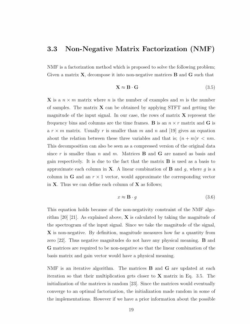
NMF is a factorization method which is proposed to solve the following problem;

Given a matrix X, decompose it into non-negative matrices B and G such that

X ≈ B ·G (3.5)

X is a n × m matrix where n is the number of examples and m is the number

of samples. The matrix X can be obtained by applying STFT and getting the

magnitude of the input signal. In our case, the rows of matrix X represent the

frequency bins and columns are the time frames. B is an n× r matrix and G is

a r × m matrix. Usually r is smaller than m and n and [19] gives an equation

about the relation between these three variables and that is; (n + m)r < nm.

This decomposition can also be seen as a compressed version of the original data

since r is smaller than n and m. Matrices B and G are named as basis and

gain respectively. It is due to the fact that the matrix B is used as a basis to

approximate each column in X. A linear combination of B and g, where g is a

column in G and an r × 1 vector, would approximate the corresponding vector

in X. Thus we can define each column of X as follows;

x ≈ B · g (3.6)

This equation holds because of the non-negativity constraint of the NMF algo-

rithm [20] [21]. As explained above, X is calculated by taking the magnitude of

the spectrogram of the input signal. Since we take the magnitude of the signal,

X is non-negative. By definition, magnitude measures how far a quantity from

zero [22]. Thus negative magnitudes do not have any physical meaning. B and

G matrices are required to be non-negative so that the linear combination of the

basis matrix and gain vector would have a physical meaning.

NMF is an iterative algorithm. The matrices B and G are updated at each

iteration so that their multiplication gets closer to X matrix in Eq. 3.5. The

initialization of the matrices is random [23]. Since the matrices would eventually

converge to an optimal factorization, the initialization made random in some of

the implementations. However if we have a prior information about the possible

19

decomposition (e.g. sparseness of the data), the matrices can be also initialized

in favor the prior knowledge.

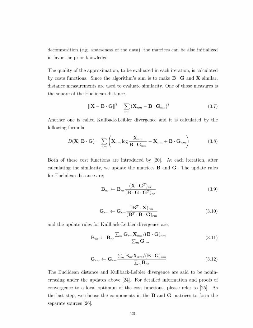
The quality of the approximation, to be evaluated in each iteration, is calculated

by costs functions. Since the algorithm’s aim is to make B · G and X similar,

distance measurements are used to evaluate similarity. One of those measures is

the square of the Euclidean distance.

||X−B ·G||2 =∑nm

(Xnm −B ·Gnm)2 (3.7)

Another one is called Kullback-Leibler divergence and it is calculated by the

following formula;

D(X||B ·G) =∑nm

(Xnm log

Xnm

B ·Gnm

−Xnm + B ·Gnm

)(3.8)

Both of these cost functions are introduced by [20]. At each iteration, after

calculating the similarity, we update the matrices B and G. The update rules

for Euclidean distance are;

Bnr ← Bnr(X ·GT )nr

(B ·G ·GT )nr(3.9)

Grm ← Grm(BT ·X)rm

(BT ·B ·G)rm(3.10)

and the update rules for Kullback-Leibler divergence are;

Bnr ← Bnr

∑m GrmXnm/(B ·G)nm∑

m Grm

(3.11)

Grm ← Grm

∑nBnrXnm/(B ·G)nm∑

nBnr

(3.12)

The Euclidean distance and Kullback-Leibler divergence are said to be nonin-

creasing under the updates above [24]. For detailed information and proofs of

convergence to a local optimum of the cost functions, please refer to [25]. As

the last step, we choose the components in the B and G matrices to form the

separate sources [26].

20

3.4 Non-Negative Tensor Factorization (NTF)

Non-negative Tensor Factorization is very similar to NMF. NTF introduces an-

other dimension for the data representation [27]. While NMF decomposes a

magnitude or power spectrum basis over time varying gain, NTF uses modula-

tion domain as the third dimension and includes frequency varying activation.

Since our aim is to use the modulation domain information of the instruments,

we adopt NTF to separate over the modulation domain. The NTF algorithm gets

a tensor as input. A tensor is a three dimensional array where the dimensions

represent frequency, time and modulation. Let the tensor be represented as X.

Then the purpose of NTF is to decompose X into G, A and S matrices.

Xr,n,m ≈ Xr,n,m =K∑k=1

Gr,k ·An,k · Sm,k (3.13)

where G, A and S are gain, frequency basis and activation, respectively. The

initialization of the matrices is often random, as it is in NMF. In some cases, it is

better to initialize the matrices with respect to a prior knowledge. NTF is also an

iterative algorithm. At each iteration, the matrices G, A and S are updated at

each iteration depending on how close the approximation in Eq. 3.13 has become.

The update rules are determined according to the cost function. Kullnack-Leibler

divergence and Euclidean distance can be used in NTF. The equations can be

easily derived from 3.7 and 3.8. However we give the equation for KL divergence

since we use it in the implementation.

D(X ‖ X) =∑r,n,m

logXr,n,m

Xr,n,m

−Xr,n,m + Xr,n,m (3.14)

The update rules for the KL divergence cost functions is as follows;

Gr,k ← Gr,k

∑n,mCr,n,m ·An,k · Sm,k∑

n,m An,k · Sm,k

(3.15)

An,k ← An,k

∑r,m Cr,n,m ·Gr,k · Sm,k∑

r,m Gr,k · Sm,k

(3.16)

Sm,k ← Sm,k

∑r,n Cr,n,m ·Gr,k ·An,k∑

r,n Gr,k ·An,k

(3.17)

21

G, A and S matrices contain many useful information. Matrix G is called basis

and contains the frequency spectrum information. Matrix A contains modulation

domain information and matrix S is called activation; it shows in which time

those frequencies are active. Notice all three have k columns. The value of k is

a user defined parameter and it is called the number of components. If we look

from the source separation point of view, we expect the sources to be separated.

When we have two sources in the mixture, if we define k = 2, it means G, A

and S matrices have 2 columns and we expect from the algorithm to put all the

frequency, modulation and activation information of a source into one column of

G, A and S respectively and the other column should have all the information

for the other source. For the cases where k is bigger than the number of sources,

each component is expected to have one particular information that belongs to one

source only. That information is most likely a portion of the frequency spectrum

of the source over a time frame. So when k is bigger than the number of sources,

a source’s information is most likely divided into many components. In that case

we should cluster the components before synthesizing the source. Choosing the

right k depends on the mixture; how many instruments are involved, how well are

the sources mixed, etc are some of the important criteria to consider. Since it is

hard to estimate the best value of k, the best option is to experiment on different

values of k. In chapter 4 we present what we have observed by experimenting on

the values of k. Other than the correct k value, it is also important to determine

a reasonable iteration number. Less then required number of iteration would end

up with an unsuccessful separation and more iteration would mean overfitting or

slower processing.

3.5 Computational Auditory Scene Analysis

(CASA)

CASA is a research field that deals with computational examination of the sounds

in an environment [28]. One of those separation methods is the CAM (Common

22

Amplitude Modulation) method [29]. This is the very first algorithm that we

have tried when we decided to work on musical instrument source separation.

However our studies showed that we cannot apply this methodology on unison

musical source separation case. The CAM methodology is based on the fact

that the amplitude of the harmonics of an instrument tends to have a similar

spectral shape. There exists a source separation method for monaural mixtures

[30] uses CAM to perform separation. The system classifies all the harmonics in a

spectrogram as non-overlapped or overlapped by using the fundamental frequency

values of the instruments. After that, it discards all the non-overlapped harmonics

since there is no feasible way to separate that harmonic. Then it re-creates that

harmonic for both instruments by the CAM principle; which is to estimate the

shape of the amplitude modulation over time by the neighboring harmonics of

the instruments.

This method requires having different pitches of both instruments in the mixture.

For the unison case, since both instruments are played at the same pitch, almost

all the harmonics would be overlapped. So there would be no way to obtain

the spectral shape of the amplitude of the harmonics. In order to modify this

algorithm for the unison case, one can use model based algorithms to estimate a

spectral shape for all the possible instruments that would appear in the mixture.

However, since the spectral shape of the harmonics amplitudes depend on many

aspects like recording environment, style, playing style. It would be hard to build

a model that covers all those different aspects. Therefore we decided not to work

further with CAM method.

23

Chapter 4

The NTF Based Source

Separation Algorithm

Most source separation algorithms are proposed for a specific problem domain. As

in research areas like machine learning or pattern recognition, an algorithm that

works fine for all cases does not exist. Within all the possible problem domains, we

decided to work on a base case as if we are solving a recursive problem. If we look

close enough to a spectrogram of an unison instrument mixture, we eventually

would find those two instruments playing at a constant tone. We decided to work

on these small time intervals and we assumed that this problem domain can be

seen as the base case of the bigger problem. Investigating on this base case might

reveal a solution to a more general source separation problem. This is our initial

motivation about working in source separation.

In this chapter we will present our proposed algorithm, our experiments and

observations and the results. We have implemented various source separation

algorithms derived from NMF and NTF and we have experimented with these

algorithms on their success with different musical instrument mixing scenarios

and different implementation techniques. Given the fact that the success of these

algorithms highly depend on initialization of the decomposition matrices and

many other parameters, we decided to observe the effects of changes in these

24

parameters and other early decisions in the source separation algorithms. So

the purpose of the implemented system is to investigate which source separation

algorithm can work better with which parameters, which instrument mixtures

and which clustering methodologies. As we expressed earlier we experiment on

combining several statistical source separation algorithms with clustering meth-

ods. The main idea is to try these methods on unison mixture case to observe

which algorithms would be successful. Some of the unison instrument mixtures

has amplitude modulation added to one or both of their instruments. We expect

amplitude modulation detection based separation methods to work better with

these mixtures. Rest of this chapter will introduce the detailed explanation of

the algorithms, our musical instruments and the listening test.

4.1 The NTF Based Algorithm

The algorithm that we have proposed is based on the NTF algorithm. Figure 4.1

shows the block diagram of the algorithm. It visualizes each step of the separation

process. The following section explains the building blocks of the system. The

algorithm starts with zero padding. As explained in the previous chapter, zero

padding adds zeros to the beginning and end of the signal. We need this in order

to prevent getting noisy peaks in the frequency domain.

4.1.1 DFT Filterbank

We apply a filterbank in order to divide the frequency spectrum into bins. Within

the source separation algorithms, one can use many different filterbanks including

gammatone and DFT filterbanks. A DFT filterbank divides the spectrogram into

equal sized bins whereas a gammatone filterbank mimics the human auditory

system on grouping the frequencies into bins [27]. In our algorithm we use a

DFT filterbank. We use STFT to apply the DFT filterbank. The challenging

task is to calculate the best window size so that the all the frequency peaks,

which are the fundamental frequency and the harmonics, are at the center or

25

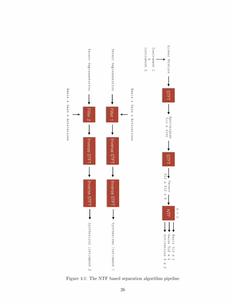
Figure 4.1: The NTF based separation algorithm pipeline

26

0 500 1000 1500 2000 25000

5

10

15

20

25

30

35

40

45

50

frequency (Hz)

Magnitude

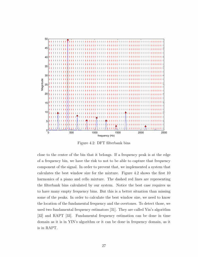
Figure 4.2: DFT filterbank bins

close to the center of the bin that it belongs. If a frequency peak is at the edge

of a frequency bin, we have the risk to not to be able to capture that frequency

component of the signal. In order to prevent that, we implemented a system that

calculates the best window size for the mixture. Figure 4.2 shows the first 10

harmonics of a piano and cello mixture. The dashed red lines are representing

the filterbank bins calculated by our system. Notice the best case requires us

to have many empty frequency bins. But this is a better situation than missing

some of the peaks. In order to calculate the best window size, we need to know

the location of the fundamental frequency and the overtones. To detect those, we

used two fundamental frequency estimators [31]. They are called Yin’s algorithm

[32] and RAPT [33]. Fundamental frequency estimation can be done in time

domain as it is in YIN’s algorithm or it can be done in frequency domain, as it

is in RAPT.

27

0

0.5

1

1.5

2

2.5x 10

4 Basis Vectors

Fre

quency (

Hz)

Basis0

2

4

6

8

10

12

14

16

18Activation Vectors

tim

e

Activations0

0.5

1

1.5

2

2.5x 10

4 Gain Vectors

Fre

quency (

Hz)

Gains

Figure 4.3: NTF decomposition of a single sine wave

Note that STFT outputs amplitude and phase parts. We store the phase ma-

trix to be used in the reconstruction stage. After performing the separation in

modulation domain. We need to combine the phase matrix with the magnitude

matrix. Section 4.1.4 explains the reconstruction phase.

4.1.2 Tensor Representation

After dividing the frequency spectrum into bins, the next step is to produce the

tensor representation of the signal in order to work with the NTF algorithm.

Tensor representation adds another dimension that is the modulation axis. After

applying the filterbank, notice that we obtain a matrix representation of the

mixture. The rows are the filterbank bins, and the columns are the sample values.

In other words, we can define the rows as frequency axis, whereas the columns

28

0

0.5

1

1.5

2

2.5x 10

4 Basis Vectors

Fre

quency (

Hz)

Basis0

2

4

6

8

10

12

14

16

18Activation Vectors

tim

e

Activations0

0.5

1

1.5

2

2.5x 10

4 Gain Vectors

Fre

quency (

Hz)

Gains

Figure 4.4: Tensor decomposition for the mixture of two sine waves

are time axis. In figure 4.1, we apply STFT to each column of the spectrogram

representation. For a better visualization of the NTF result, we have given the

dimensions as 512 × 4096 for the spectrogram and 512 × 512 × 8 for the tensor

represenation as example values. Note that STFT reveals all of the repetitions

and patterns in the data. If frequency data is used as an input to STFT, then the

magnitude of the result would be the modulations, the rhythmic changes in the

frequency domain. Again we store the phase matrix to be used in reconstruction.

4.1.3 The NTF algorithm

After preparing the tensor representation of the mixture data, the next step is

to decompose it into Basis, Activations and Gains matrices. As explained in

29

0

0.5

1

1.5

2

2.5x 10

4 Basis Vectors

Fre

quency (

Hz)

Basis0

2

4

6

8

10

12

14

16

18Activation Vectors

tim

e

Activations0

0.5

1

1.5

2

2.5x 10

4 Gain Vectors

Fre

quency (

Hz)

Gains

Figure 4.5: Tensor decomposition for the mixture of two sine waves with AM

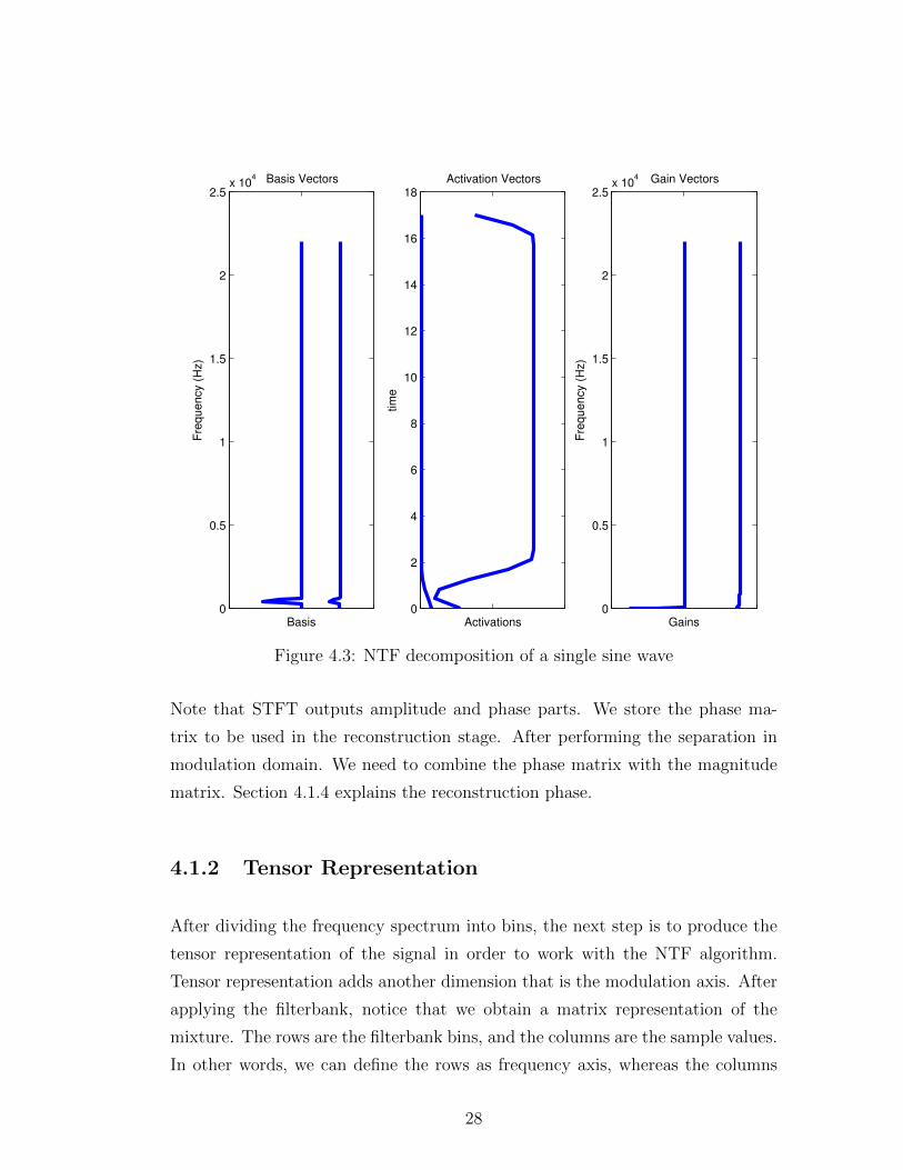
the previous chapter, we use NTF algorithm to perform this task [27]. The

output of NTF visualizes the frequency, time and modulation dimensions at the

same time. The Basis matrix shows frequency domain information, the Gains

matrix shows modulation domain information and Activations matrix shows the

time intervals that the Basis and Gains are active. Figure 4.3 shows the G,

A and S matrices for a single sine wave, that is the first case in out test files.

Notice we have two blue lines in each plot since the number of components is

set to two for that NTF run. Figure 4.1 also shows how the dimensions of those

matrices would be, when k = 2. With two components, we would expect that

each component will represent a source. If we had more number of components,

a component would represent a part of a source. This NTF run on the single

sine wave divided the power of the same frequency bin among the components.

In a successful separation we would expect one component to have the frequency

peak and the other component to have nothing. But separation success depends

30

0

0.5

1

1.5

2

2.5x 10

4 Basis Vectors

Fre

quency (

Hz)

Basis0

0.5

1

1.5

2

2.5

3

3.5

4

4.5

5Activation Vectors

tim

e

Activations0

0.5

1

1.5

2

2.5x 10

4 Gain Vectors

Fre

quency (

Hz)

Gains

Figure 4.6: Tensor decomposition for piano and cello mixture

on many factors, including the input properties and number of components. Our

experiments showed that NTF and NMF work poorly when k = 2. If the number

of the components are more than the number of sources, each component would

contain a fragment of one of the sources. Since it gives better results to select

k > 2, the source separation algorithm would separate the mixture into k many

fragments. Figure 4.7 visualizes this scenario. The solution is to cluster the

components into the number of sources. We will cover that concept later in this

chapter.

The Activations plot shows the time frames where the frequencies are active. In

Figure 4.3, the activations matrix shows that the component on the left hand side

is active all the time. For the component on the right hand side is active only

at the beginning. Finally the Gains matrix show that there are no modulation

frequencies in this sine wave. This is expected since the input sine wave does not

31

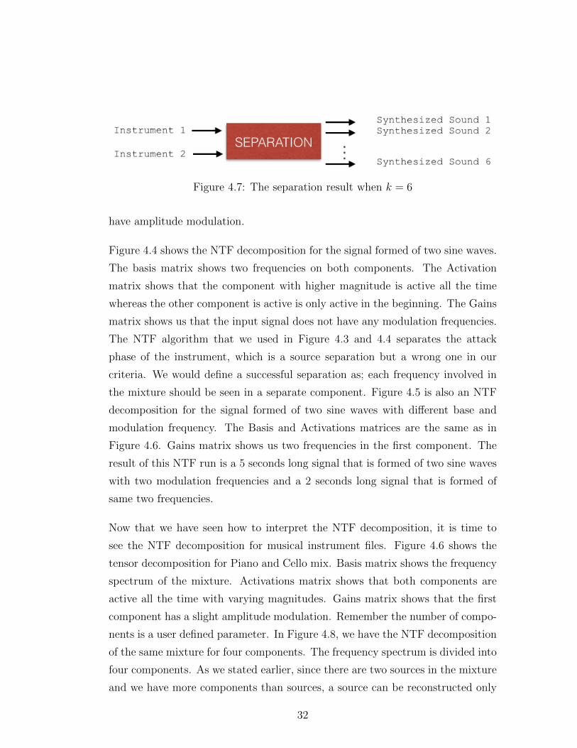
Figure 4.7: The separation result when k = 6

have amplitude modulation.

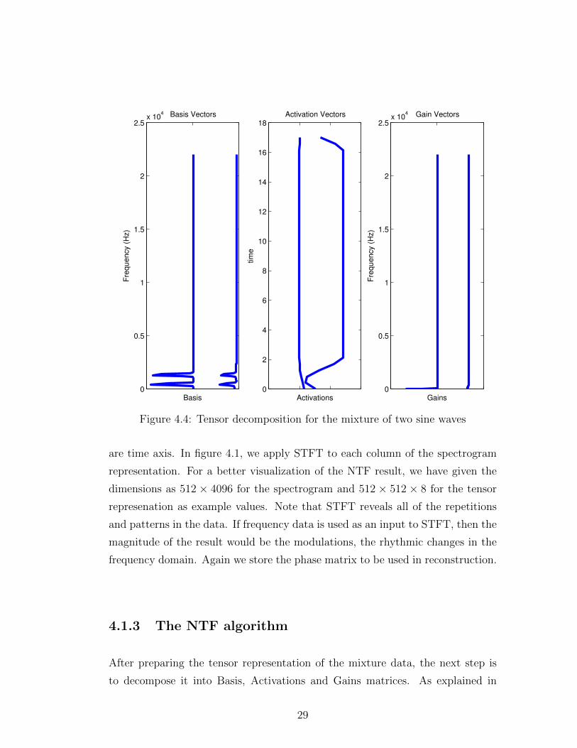
Figure 4.4 shows the NTF decomposition for the signal formed of two sine waves.

The basis matrix shows two frequencies on both components. The Activation

matrix shows that the component with higher magnitude is active all the time

whereas the other component is active is only active in the beginning. The Gains

matrix shows us that the input signal does not have any modulation frequencies.

The NTF algorithm that we used in Figure 4.3 and 4.4 separates the attack

phase of the instrument, which is a source separation but a wrong one in our

criteria. We would define a successful separation as; each frequency involved in

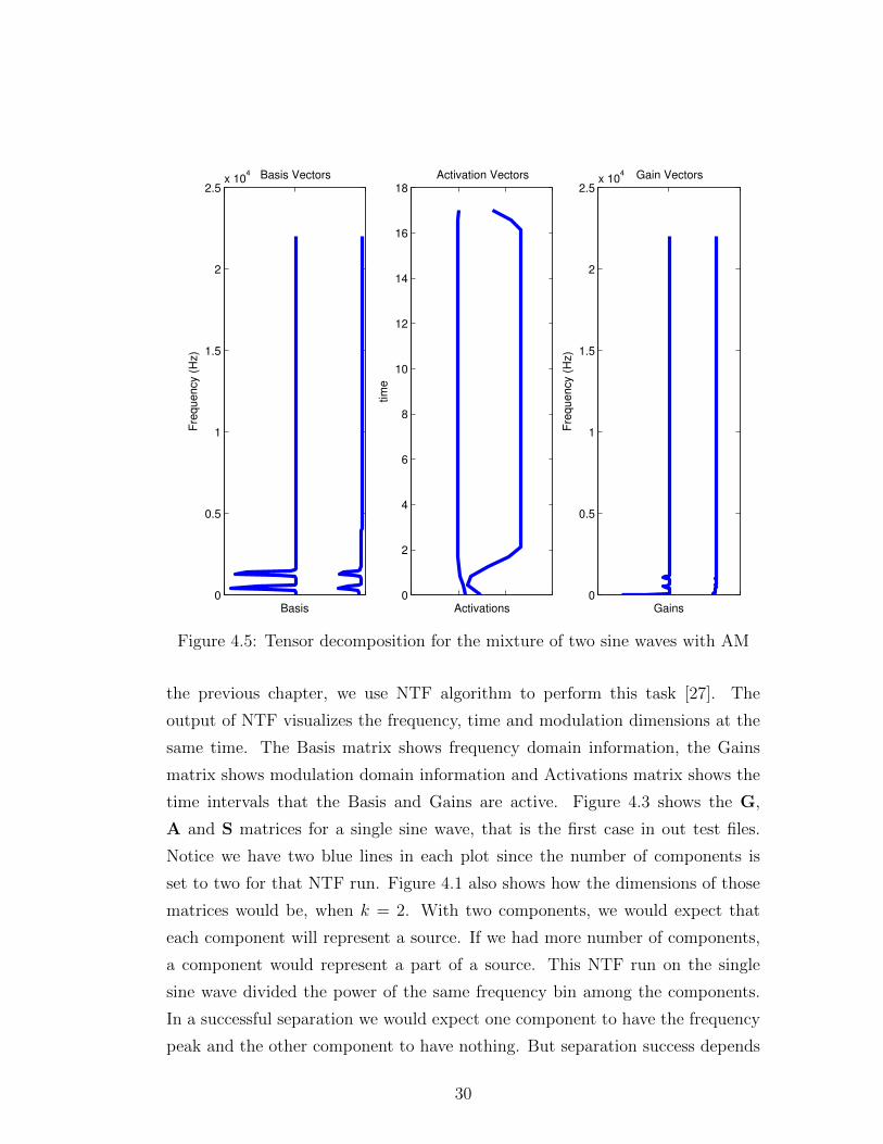
the mixture should be seen in a separate component. Figure 4.5 is also an NTF

decomposition for the signal formed of two sine waves with different base and

modulation frequency. The Basis and Activations matrices are the same as in

Figure 4.6. Gains matrix shows us two frequencies in the first component. The

result of this NTF run is a 5 seconds long signal that is formed of two sine waves

with two modulation frequencies and a 2 seconds long signal that is formed of

same two frequencies.

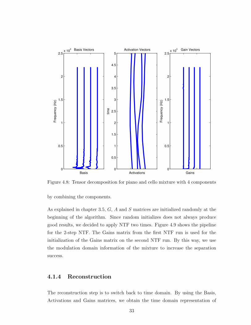
Now that we have seen how to interpret the NTF decomposition, it is time to

see the NTF decomposition for musical instrument files. Figure 4.6 shows the

tensor decomposition for Piano and Cello mix. Basis matrix shows the frequency

spectrum of the mixture. Activations matrix shows that both components are

active all the time with varying magnitudes. Gains matrix shows that the first

component has a slight amplitude modulation. Remember the number of compo-

nents is a user defined parameter. In Figure 4.8, we have the NTF decomposition

of the same mixture for four components. The frequency spectrum is divided into

four components. As we stated earlier, since there are two sources in the mixture

and we have more components than sources, a source can be reconstructed only

32

0

0.5

1

1.5

2

2.5x 10

4 Basis Vectors

Fre

quency (

Hz)

Basis0

0.5

1

1.5

2

2.5

3

3.5

4

4.5

5Activation Vectors

tim

e

Activations0

0.5

1

1.5

2

2.5x 10

4 Gain Vectors

Fre

quency (

Hz)

Gains

Figure 4.8: Tensor decomposition for piano and cello mixture with 4 components

by combining the components.

As explained in chapter 3.5, G, A and S matrices are initialized randomly at the

beginning of the algorithm. Since random initializes does not always produce

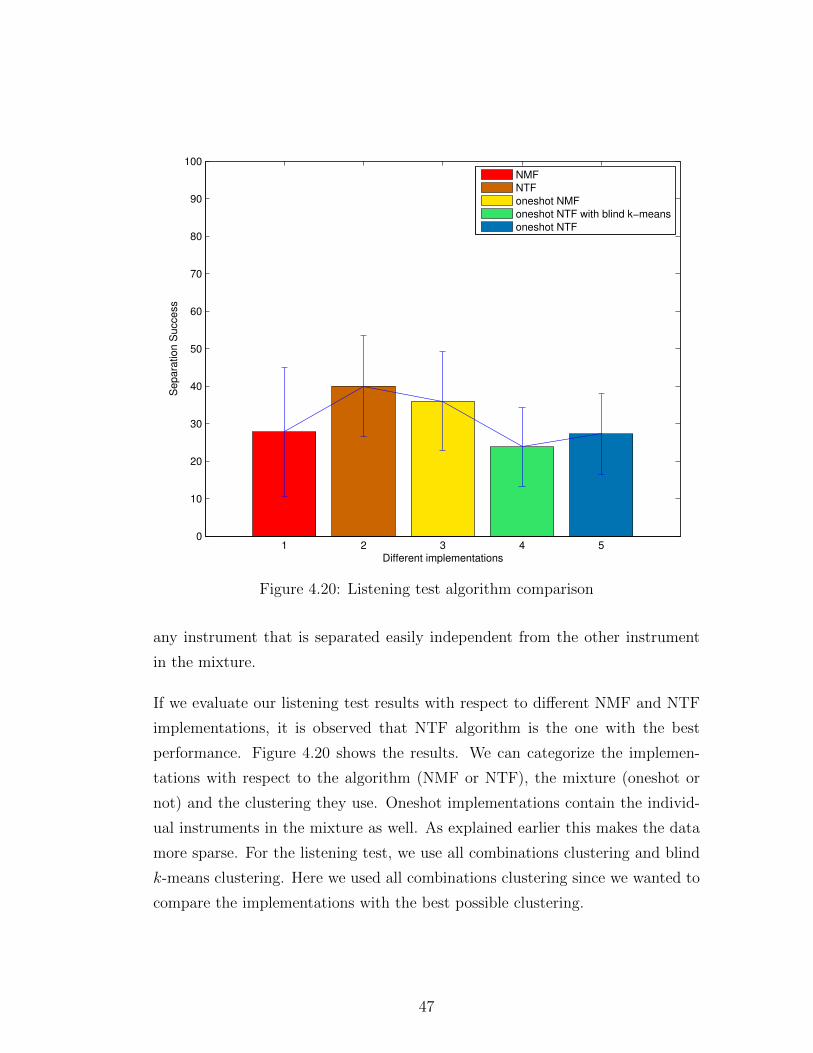
good results, we decided to apply NTF two times. Figure 4.9 shows the pipeline

for the 2-step NTF. The Gains matrix from the first NTF run is used for the

initialization of the Gains matrix on the second NTF run. By this way, we use

the modulation domain information of the mixture to increase the separation

success.

4.1.4 Reconstruction

The reconstruction step is to switch back to time domain. By using the Basis,

Activations and Gains matrices, we obtain the time domain representation of

33

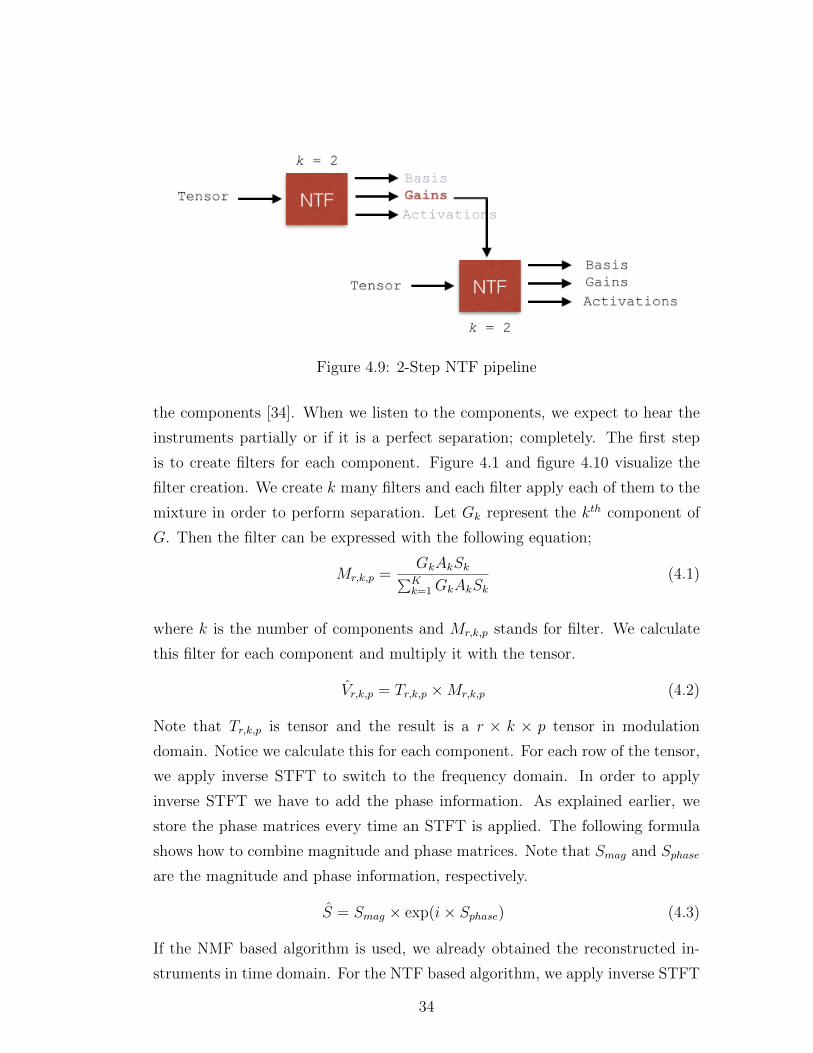
Figure 4.9: 2-Step NTF pipeline

the components [34]. When we listen to the components, we expect to hear the

instruments partially or if it is a perfect separation; completely. The first step

is to create filters for each component. Figure 4.1 and figure 4.10 visualize the

filter creation. We create k many filters and each filter apply each of them to the

mixture in order to perform separation. Let Gk represent the kth component of

G. Then the filter can be expressed with the following equation;

Mr,k,p =GkAkSk∑Kk=1GkAkSk

(4.1)

where k is the number of components and Mr,k,p stands for filter. We calculate

this filter for each component and multiply it with the tensor.

Vr,k,p = Tr,k,p ×Mr,k,p (4.2)

Note that Tr,k,p is tensor and the result is a r × k × p tensor in modulation

domain. Notice we calculate this for each component. For each row of the tensor,

we apply inverse STFT to switch to the frequency domain. In order to apply

inverse STFT we have to add the phase information. As explained earlier, we

store the phase matrices every time an STFT is applied. The following formula

shows how to combine magnitude and phase matrices. Note that Smag and Sphase

are the magnitude and phase information, respectively.

S = Smag × exp(i× Sphase) (4.3)

If the NMF based algorithm is used, we already obtained the reconstructed in-

struments in time domain. For the NTF based algorithm, we apply inverse STFT

34

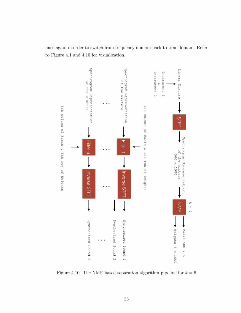
once again in order to switch from frequency domain back to time domain. Refer

to Figure 4.1 and 4.10 for visualization.

Figure 4.10: The NMF based separation algorithm pipeline for k = 6

35

4.1.5 Clustering

The reconstruction step prepares the time domain representation of the compo-

nents. As we explained earlier, when we have more components than the number

of sources, components have partial information about the instruments and we

add them up to have the complete spectra of the sources. But deciding which

component belongs to which source is challenging. Since NMF and NTF al-

gorithms do not perform a perfect decomposition, a component would contain

information from both instrument’s frequency spectrum. Thus, the task is to

evaluate the similarity of the components to sources. An unsupervised algorithm

will not be able to use any prior information about the sources whereas a super-

vised algorithm can compare the components with the original sources in order

to see the best case clustering scenario. In this thesis we experimented with var-

ious clustering algorithms including both supervised and unsupervised clustering

approaches.

We used k-means as our main clustering algorithm. K-means algorithm clusters

the components such that the overall euclidean distance between the elements

in each cluster are minimum [27] [35]. We used k-means both in supervised

and unsupervised cases. We also use a similarity measurement called Signal to

Distortion Ratio (SDR) to perform clustering [36]. Let’s introduce the clustering

methodologies that we used.

Signal to Distortion Ratio (SDR): Blind SDR clustering calculates similarity

for each component pair combination and clusters the components with respect

to similarity values. Number of clusters is always set to number of sources.

Supervised SDR: In supervised SDR we use the original sources. Each compo-

nent is compared with both of the sources and similarity is calculated with SDR.

Then each component is clustered with respect to which cluster they are more

similar to.

Blind K-means: We use Blind k-means with respect to Basis and Gain matri-

ces. Remember Basis and Gain matrices hold frequency and modulation domain

36

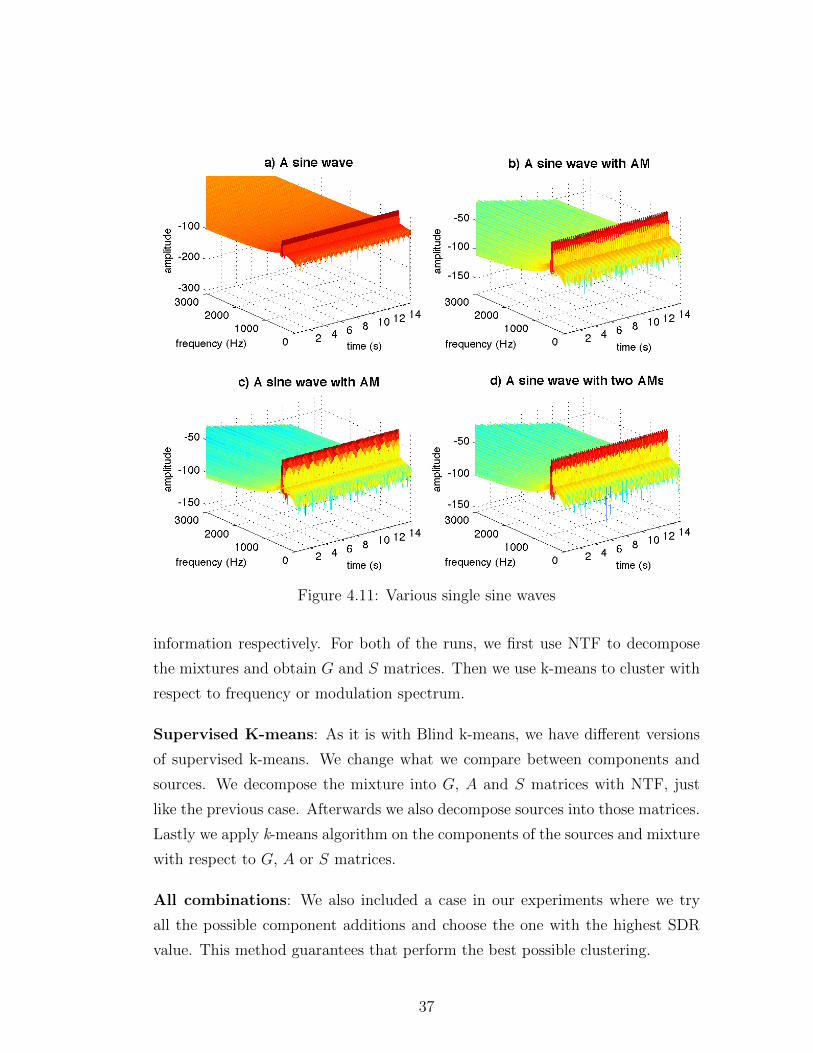
Figure 4.11: Various single sine waves

information respectively. For both of the runs, we first use NTF to decompose

the mixtures and obtain G and S matrices. Then we use k-means to cluster with

respect to frequency or modulation spectrum.

Supervised K-means: As it is with Blind k-means, we have different versions

of supervised k-means. We change what we compare between components and

sources. We decompose the mixture into G, A and S matrices with NTF, just

like the previous case. Afterwards we also decompose sources into those matrices.

Lastly we apply k-means algorithm on the components of the sources and mixture

with respect to G, A or S matrices.

All combinations: We also included a case in our experiments where we try

all the possible component additions and choose the one with the highest SDR

value. This method guarantees that perform the best possible clustering.

37

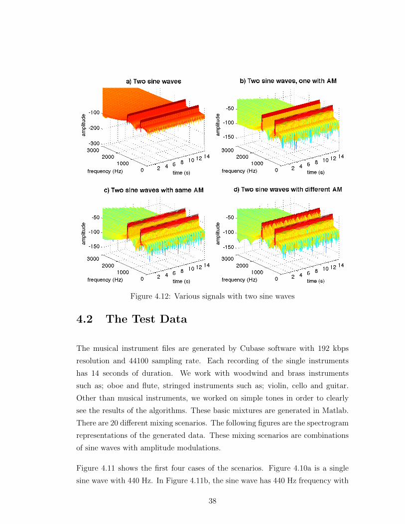
Figure 4.12: Various signals with two sine waves

4.2 The Test Data

The musical instrument files are generated by Cubase software with 192 kbps

resolution and 44100 sampling rate. Each recording of the single instruments

has 14 seconds of duration. We work with woodwind and brass instruments

such as; oboe and flute, stringed instruments such as; violin, cello and guitar.

Other than musical instruments, we worked on simple tones in order to clearly

see the results of the algorithms. These basic mixtures are generated in Matlab.

There are 20 different mixing scenarios. The following figures are the spectrogram

representations of the generated data. These mixing scenarios are combinations

of sine waves with amplitude modulations.

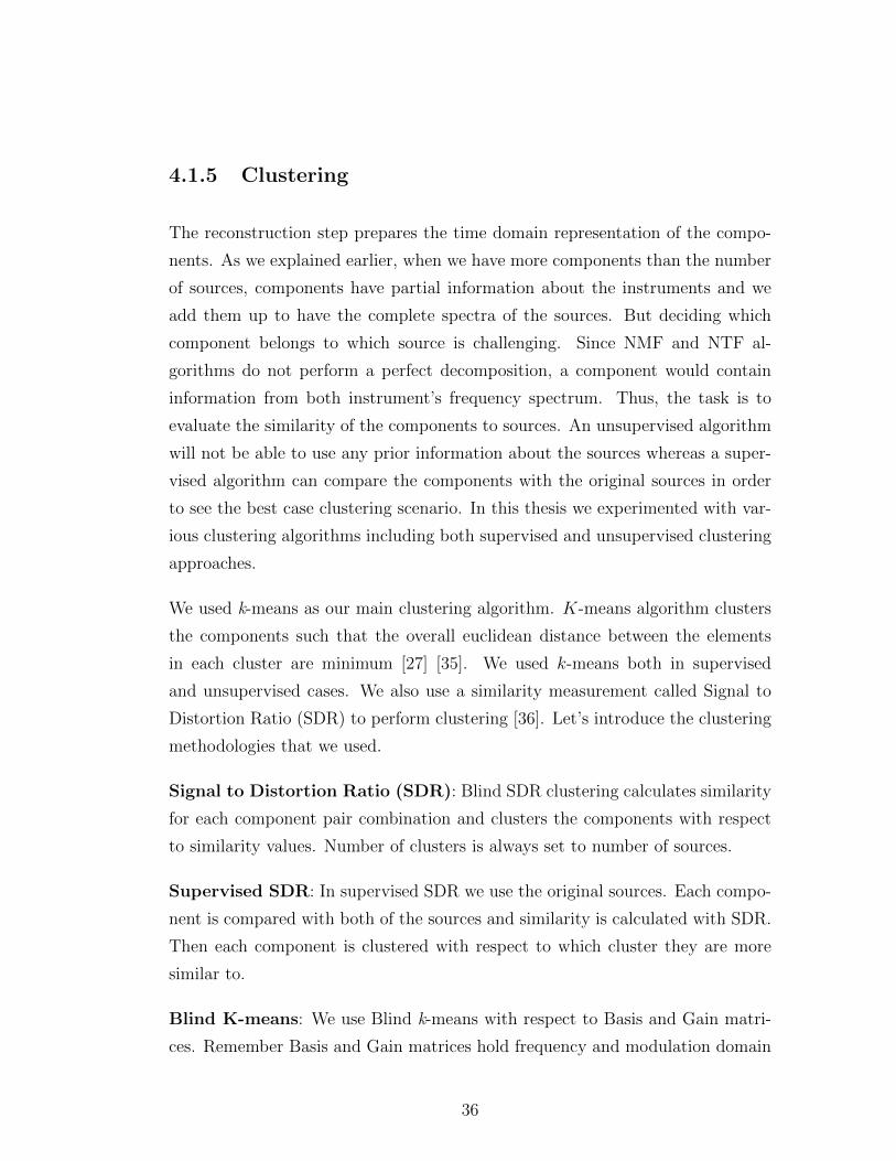
Figure 4.11 shows the first four cases of the scenarios. Figure 4.10a is a single

sine wave with 440 Hz. In Figure 4.11b, the sine wave has 440 Hz frequency with

38

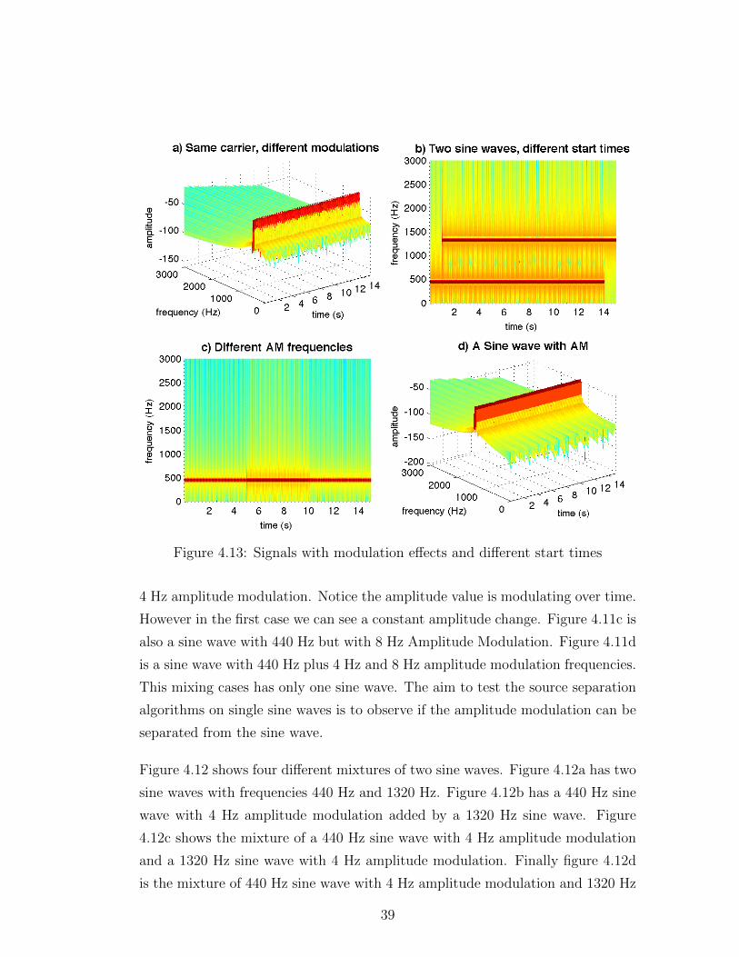
Figure 4.13: Signals with modulation effects and different start times

4 Hz amplitude modulation. Notice the amplitude value is modulating over time.

However in the first case we can see a constant amplitude change. Figure 4.11c is

also a sine wave with 440 Hz but with 8 Hz Amplitude Modulation. Figure 4.11d

is a sine wave with 440 Hz plus 4 Hz and 8 Hz amplitude modulation frequencies.

This mixing cases has only one sine wave. The aim to test the source separation

algorithms on single sine waves is to observe if the amplitude modulation can be

separated from the sine wave.

Figure 4.12 shows four different mixtures of two sine waves. Figure 4.12a has two

sine waves with frequencies 440 Hz and 1320 Hz. Figure 4.12b has a 440 Hz sine

wave with 4 Hz amplitude modulation added by a 1320 Hz sine wave. Figure

4.12c shows the mixture of a 440 Hz sine wave with 4 Hz amplitude modulation

and a 1320 Hz sine wave with 4 Hz amplitude modulation. Finally figure 4.12d

is the mixture of 440 Hz sine wave with 4 Hz amplitude modulation and 1320 Hz

39

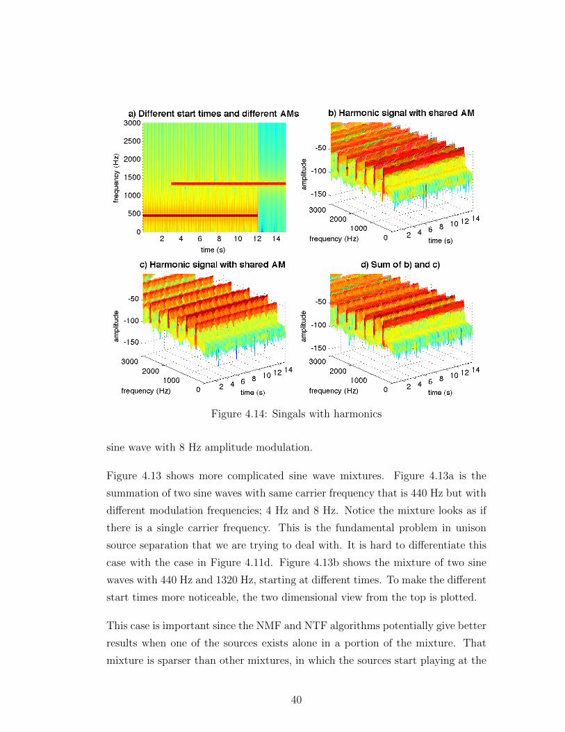
Figure 4.14: Singals with harmonics

sine wave with 8 Hz amplitude modulation.

Figure 4.13 shows more complicated sine wave mixtures. Figure 4.13a is the

summation of two sine waves with same carrier frequency that is 440 Hz but with

different modulation frequencies; 4 Hz and 8 Hz. Notice the mixture looks as if

there is a single carrier frequency. This is the fundamental problem in unison

source separation that we are trying to deal with. It is hard to differentiate this

case with the case in Figure 4.11d. Figure 4.13b shows the mixture of two sine

waves with 440 Hz and 1320 Hz, starting at different times. To make the different

start times more noticeable, the two dimensional view from the top is plotted.

This case is important since the NMF and NTF algorithms potentially give better

results when one of the sources exists alone in a portion of the mixture. That

mixture is sparser than other mixtures, in which the sources start playing at the

40

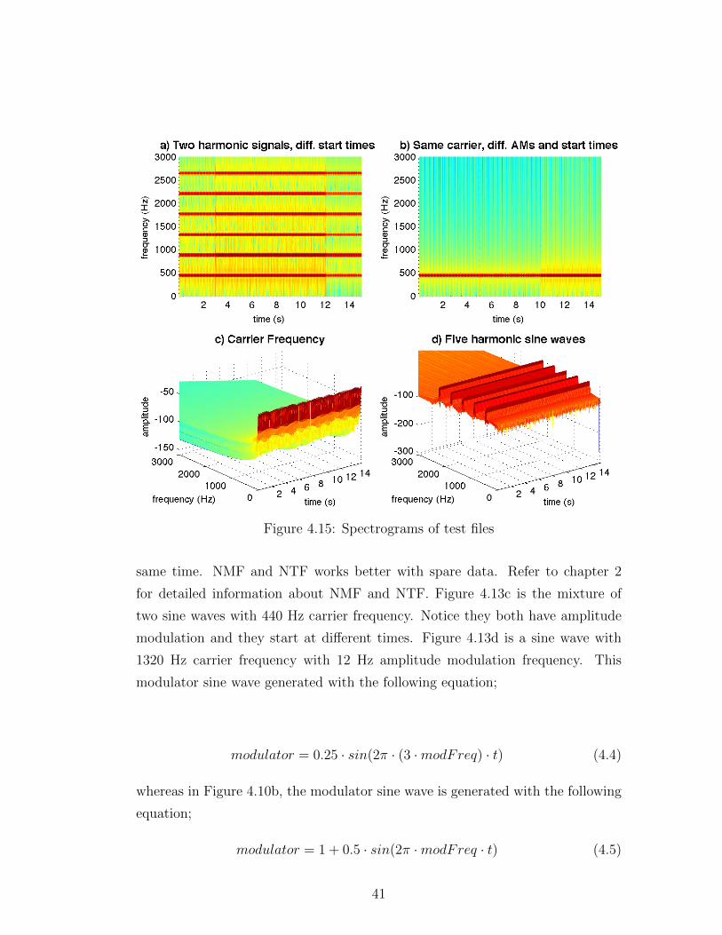
Figure 4.15: Spectrograms of test files

same time. NMF and NTF works better with spare data. Refer to chapter 2

for detailed information about NMF and NTF. Figure 4.13c is the mixture of

two sine waves with 440 Hz carrier frequency. Notice they both have amplitude

modulation and they start at different times. Figure 4.13d is a sine wave with

1320 Hz carrier frequency with 12 Hz amplitude modulation frequency. This

modulator sine wave generated with the following equation;

modulator = 0.25 · sin(2π · (3 ·modFreq) · t) (4.4)

whereas in Figure 4.10b, the modulator sine wave is generated with the following

equation;

modulator = 1 + 0.5 · sin(2π ·modFreq · t) (4.5)

41

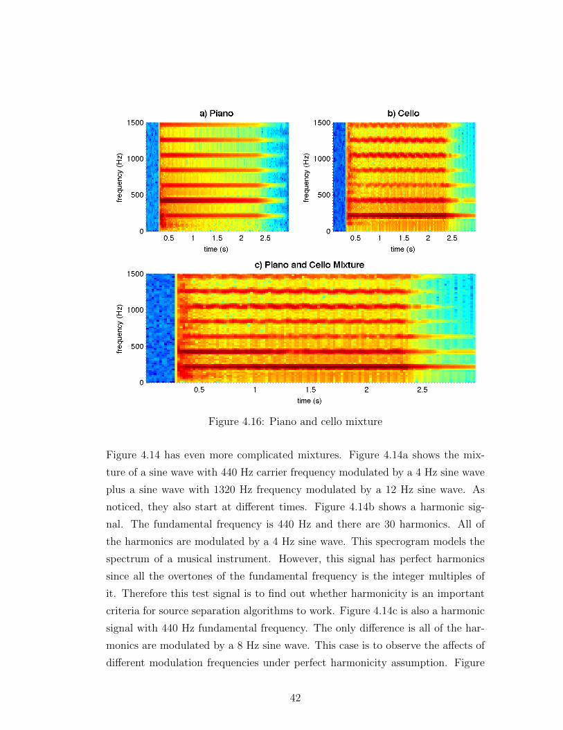
Figure 4.16: Piano and cello mixture

Figure 4.14 has even more complicated mixtures. Figure 4.14a shows the mix-

ture of a sine wave with 440 Hz carrier frequency modulated by a 4 Hz sine wave

plus a sine wave with 1320 Hz frequency modulated by a 12 Hz sine wave. As

noticed, they also start at different times. Figure 4.14b shows a harmonic sig-

nal. The fundamental frequency is 440 Hz and there are 30 harmonics. All of

the harmonics are modulated by a 4 Hz sine wave. This specrogram models the

spectrum of a musical instrument. However, this signal has perfect harmonics

since all the overtones of the fundamental frequency is the integer multiples of

it. Therefore this test signal is to find out whether harmonicity is an important

criteria for source separation algorithms to work. Figure 4.14c is also a harmonic

signal with 440 Hz fundamental frequency. The only difference is all of the har-

monics are modulated by a 8 Hz sine wave. This case is to observe the affects of

different modulation frequencies under perfect harmonicity assumption. Figure

42

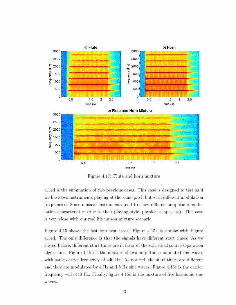
Figure 4.17: Flute and horn mixture

4.14d is the summation of two previous cases. This case is designed to test as if

we have two instruments playing at the same pitch but with different modulation

frequencies. Since musical instruments tend to show different amplitude modu-

lation characteristics (due to their playing style, physical shape, etc). This case

is very close with our real life unison mixture scenario.

Figure 4.15 shows the last four test cases. Figure 4.15a is similar with Figure

4.14d. The only difference is that the signals have different start times. As we

stated before, different start times are in favor of the statistical source separation

algorithms. Figure 4.15b is the mixture of two amplitude modulated sine waves

with same carrier frequency of 440 Hz. As noticed, the start times are different

and they are modulated by 4 Hz and 8 Hz sine waves. Figure 4.15c is the carrier

frequency with 440 Hz. Finally, figure 4.15d is the mixture of five harmonic sine

waves.

43

Figure 4.18: Oboe and violin mixture

As stated earlier, we work on generated musical instrument mixes as well. In

our initial experiments, we have worked on three different instrument mixes.

Those pairs are, piano and cello, flute and horn and violin and oboe. We used

these mixtures in our early experiments. For the final experiment with the final

version of the algorithm, we have used 11 instruments and their 55 pair-wise

combinations.

Figure 4.16 shows the spectrograms of a piano, a cello and their mixture. Notice

this is the 2D representation of the spectrogram. The amplitude information can

still be observed from the color changes. Darker colors indicate higher amplitude.

They play at the same pitch and they start playing at the same time. Notice

that the piano harmonics have smooth amplitude whereas cello has amplitude

modulation which can be observed from the fluctuation of the amplitude of the

harmonics. Notice further that piano has a strong attack phase which can be

44

told by observing the color changes over time. The amplitudes of the overtones

slowly looses energy over time. Cello’s attack phase is slower and wider. During

the sustain phase, the amplitude does not loose energy. These are the spectral

feature differences of these instruments. Interestingly, the mixture spectrogram

is dominated by cello. The mixture resembles cello more than it resembles piano.

This brings us to the conclusion that it is not a good way of separating the sources

by looking for the spectral characteristics of the instruments.

Figure 4.17 shows the spectrograms of a flute, a horn and their mixture. They play

at the same pitch and they start playing at the same time. When we compare

the spectrograms, we can again observe differences in spectral features. Flute

has a slower attack phase and has more amplitude modulation than Horn. In

the mixture flute looks more dominant in terms of amplitude envelope. Finally,

figure 4.18 shows the spectrograms of an oboe, a violin and their mixture. They

also play at the same pitch and they start playing at the same time. Oboe has

more amplitude modulation whereas violin have higher amplitude value. Lastly,

oboe is the dominant instrument in the mixture. We have introduced our sound

files and instruments. Our aim on choosing these instruments is to cover a wide

range of musical instrument characteristics.

4.3 Experiment and Results

This section explains the listening test and the results of it. Moreover, we sum-

marize the proposed algorithm and point out its strong and the weak points.

4.3.1 Performance Evaluation

We have performed a listening test by using 11 instrument pairs. 20 people from

Fraunhofer IIS Audiolabs have participated in the listening test. It is an online

test where the test is similar to a MUSHRA [37] test with a minor difference

which is the absence of a hidden anchor. The MUSHRA test is used to evaluate

45

0 2 4 6 8 10 12 14 16 180

10

20

30

40

50

60

70

80

90

100

Instruments

Sim

ilarity

to the o

rigin

al in

str

um

ents

Other Instruments

Violin in the Piano & Violin Mixture

Violin in the Oboe & Violin Mixture

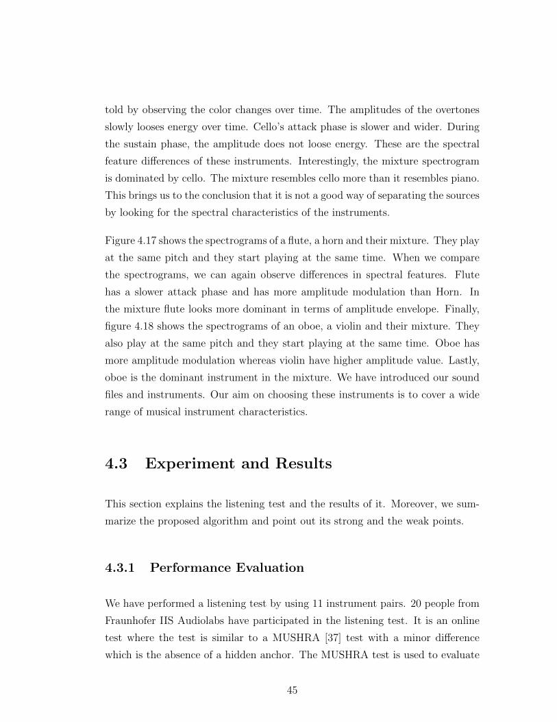
Figure 4.19: Listening test instrument comparison

the success of an audio coding algorithm. The test subjects are asked to identify

noise artifacts, which can be caused by the audio coding algorithms. If the test

subjects can not recognize any noise, the audio coding algorithm is considered

as a successful algorithm. The last detail we should give about the MUSHRA

test is the procedure of the test. For each audio signal, there are 5 audio files to

be compared with the original instrument recording. Each of those 5 audio files

are generated by using a different version of NMF or NTF. Our first aim was

to experiment on the effects of different implementations. Our results show that

there is not any significance difference between the different implementations.

However, we have found out that the test participants evaluated the separation

of violin in the piano & violin mixture as the best one. Interestingly, same

violin recording evaluated to be the worst separation result in the oboe & violin

mixture. Figure 4.19 shows these results. We conclude that separation success

is dependent on the individual instruments that are mixed. There does not exist

46

1 2 3 4 50

10

20

30

40

50

60

70

80

90

100

Different implementations

Separa

tion S

uccess

NMF

NTF

oneshot NMF

oneshot NTF with blind k−means

oneshot NTF

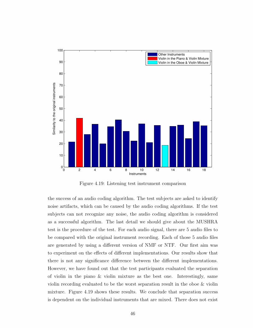
Figure 4.20: Listening test algorithm comparison

any instrument that is separated easily independent from the other instrument

in the mixture.

If we evaluate our listening test results with respect to different NMF and NTF

implementations, it is observed that NTF algorithm is the one with the best

performance. Figure 4.20 shows the results. We can categorize the implemen-

tations with respect to the algorithm (NMF or NTF), the mixture (oneshot or

not) and the clustering they use. Oneshot implementations contain the individ-

ual instruments in the mixture as well. As explained earlier this makes the data

more sparse. For the listening test, we use all combinations clustering and blind

k-means clustering. Here we used all combinations clustering since we wanted to

compare the implementations with the best possible clustering.

47

2 3 4 5 6 7 8 9 10 11 12−4

−3

−2

−1

0

1

2

3

4

Number of Components

Avera

ge S

DR

(dB

)Clustering − Piano Cello

Blind SDR

Supervised SDR

Blind K−means w.r.t G

Blind K−means w.r.t S

Supervised K−means w.r.t G

Supervised K−means w.r.t S

Figure 4.21: Clustering results for piano and cello mixture

4.3.2 Discussion

Figure 4.21 and Figure 4.22 show that the best clustering is achieved by Super-

vised SDR. That is the limit that other clustering algorithms could reach. Our

experiments show that supervised k-means with respect to Basis works as good

as supervised SDR after k = 5. Figure 4.22 compares the clustering results for

oboe and bassoon mixture. For this mixture, the SDR values are relatively low,

indicating that the separation is as not as good as the piano and cello case. How-

ever, we can still tell that supervised k-means with respect to Basis matrix is still

the best possible clustering method for our problem.

We conclude that when the sources in the mixture start at the same time, it be-

comes hard for the NTF algorithm to perform separation. When we started one

of the sources with delay, we have observed that the separation success increased.

48

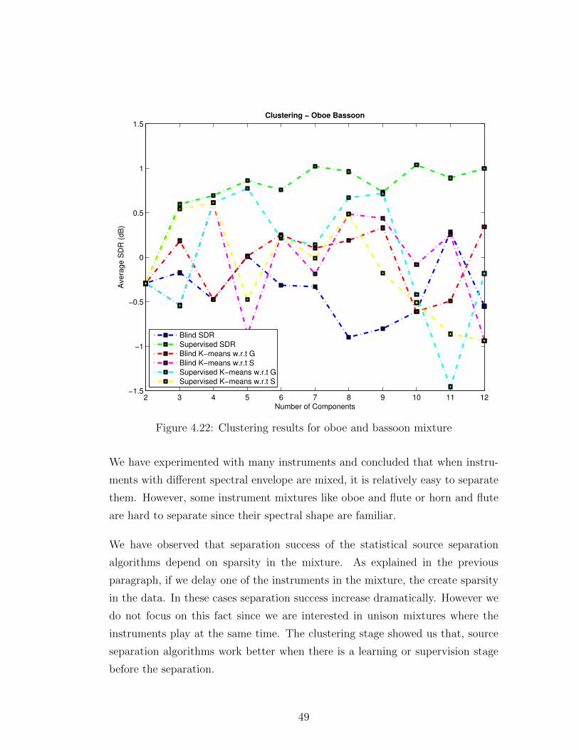
2 3 4 5 6 7 8 9 10 11 12−1.5

−1

−0.5

0

0.5

1

1.5

Number of Components

Avera

ge S

DR

(dB

)Clustering − Oboe Bassoon

Blind SDR

Supervised SDR

Blind K−means w.r.t G

Blind K−means w.r.t S

Supervised K−means w.r.t G

Supervised K−means w.r.t S

Figure 4.22: Clustering results for oboe and bassoon mixture

We have experimented with many instruments and concluded that when instru-

ments with different spectral envelope are mixed, it is relatively easy to separate

them. However, some instrument mixtures like oboe and flute or horn and flute

are hard to separate since their spectral shape are familiar.

We have observed that separation success of the statistical source separation

algorithms depend on sparsity in the mixture. As explained in the previous

paragraph, if we delay one of the instruments in the mixture, the create sparsity

in the data. In these cases separation success increase dramatically. However we

do not focus on this fact since we are interested in unison mixtures where the

instruments play at the same time. The clustering stage showed us that, source

separation algorithms work better when there is a learning or supervision stage

before the separation.

49

Chapter 5

Conclusion

Musical instrument source separation in monaural and unison recordings is a

challenging task. Unsupervised or semi-supervised source separation success is

limited since the instruments share almost all the harmonics. Stochastic source

separation algorithms such as non-negative matrix factorization (NMF) and non-

negative tensor factorization (NTF) can be used for this source separation case.

NMF and NTF is used to divide the mixture into k many fragments. NMF and

NTF works poorly when k = 2. As a result, the k value should be set to higher

values than two. When k is bigger than two, the source separation algorithms

that we have proposed output many fragments of the mixture and each fragment

contains partial information of one of the instruments. We should add the similar

fragments together until we have two sound sources. We named this step as the

clustering stage.

We have tried many different algorithms for source separation. But most of the

source separation algrithms require the mixture to be non-unison (instruments

with different start times and durations) and binaural. Thus we use NMF and

NTF as the fundamental block of our separation pipeline. We have implemented

different versions of the proposed pipeline. Some were semi-supervised in order

to see the upper limits of the unsupervised algorithms. Especially in the clus-

tering stage, we have found out that source separation success is limited without

supervised clustering algorithms.

50

To evaluate the success of our separation results, we have used the SDR similarity

measurement. Even though the separated instruments are recognizable, the SDR

values are low. Therefore we performed a listening test in order to evaluate

the separation success with respect to human auditory system perception. The

listening test showed that the some instruments are easier to recognizable after

the source separation. Moreover the source separation quality depends on the

mixture; a mixture does not necessarily have to be separated successfully just

because the individual sources of that mixture are easily recognizable.

Supervised source separation algorithms require a general knowledge of the in-

struments to be separated. We plan to combine machine learning algorithms with

our source separation algorithms. In order to use machine learning methodolo-

gies, we need to research on the timbral features that can be extracted from the

sound files.

51

Bibliography

[1] S. A. Gelfand, “Hearing: An Introduction to Psychological and Physiological

Acoustics”, fifth edition, Taylor & Francis ISBN 9781420088656, pp. 12 – 15,

2009.

[2] B. Benward and M. Saker, “Music: In Theory and Practice”, Vol. I, seventh

edition, Boston: McGraw-Hill ISBN 978-0-07-294262-0, pp. 364, 2003.

[3] A. Hyvrinen and E. Oja, “Independent component analysis: algorithms and

applications”, Neural Networks, vol 13, pp. 411 – 430, 2000.

[4] S. Haykin and Z. Chen, “The cocktail party problem”, Neural Computation,

vol. 17, pp. 1875 –1902, 2005.

[5] M. Bay, J. W. Beauchamp, “Harmonic Source Separation Using Prestored

Spectra”, 2006.

[6] J. H. McClellan, R. W. Schafer, M. A. Yoder, “Signal Processing First”,

international edition, Pearson Education International ISBN 0-13-120265-0,

pp. 7, 2003.

[7] A. P. Godse and U. A. Bakshi, “Communication Engineering”. Technical Pub-

lications, ISBN 978-81-8431-089-4, pp. 36, 2009

[8] G. Hu and D. Wang, “Monaural Speech Segregation Based on Pitch Tracking

and Amplitude Modulation”, IEEE Transactions on Neural Networks, vol 15,

no 5, pp. 1135 – 1150, 2004.

[9] X. Zhang, Z. W. Ras, “Analysis of Sound Features for Music Timbre Recog-

nition”, Multimedia and Ubiquitous Engineering, 2007.

52

[10] G. Agostini, M. Longari and E. Pollastri, “Musical Instrument Timbres Clas-

sification with Spectral Features”, EURASIP Journal on Applied Signal Pro-

cessing, 2003.

[11] E. Schubert, J. Wolfe and A. Tarnopolsky, “Special centroid and timbre in

complex, multiple”, Proceedings of the 8th International Conference on Music

Perception and Cognition, 2004.

[12] T. Virtanen, “Monaural Sound Source Separation by Nonnegative Matrix

Factorization With Temporal Continuity and Sparseness Criteria”, IEEE

Transactions on Audio, Speech and Language Processing, vol 15, no 3, pp.

1066 – 1074, 2007.

[13] A. Grecu, “Musical Instrument Separation”, Vienna University of Technol-

ogy, Master Thesis, 2007.

[14] T. Virtanen, “Signal Processing Methods for Music Transcription”, Springer

US ISBN 978-0-387-32845-4, pp. 267-296, 2006.

[15] J. S. Milton and J. C. Arnold, “Introduction to probability and statistics”,

fourth edition, McGraw Hill, pp. 156 – 164, 2003

[16] I. T. Jolliffe, “Principal Component Analysis”, Springer Series in Statistics,

second edition, 2002.

[17] G. McLachlan, “Discriminant Analysis and Statistical Pattern Recognition”,

Wiley-Interscience, ISBN 978-0471691150, 2004

[18] A. Hyvrinen and U. Kster, “FastISA: A fast fixed-point algorithm for Inde-

pendent Subspace Analysis’, 2000.

[19] B. Wang and M. D. Plumbley, “Music Audio Stream Separation by Non-

Negative Matrix Factorization”, 2005.

[20] D. D. Lee and H. S. Seung , “Algorithms for Non-negative Matrix Factor-

ization”, NIPS, 2000.

[21] D. D. Lee and S. Seung, “Learning the parts of objects by non-negative

matrix factorization”, Macmillan Magazine Ltd, vol 401, pp. 788 – 791, 1999.

53

[22] D. D. Lee and H. S. Seung, “Algorithms for Non-negative Matrix Factor-

izaiton”, MIT Press, pp. 556 –562, 2000.

[23] A. N. Langville, C. D. Meyer and R. Albright, “Initializations for the Non-

negative Matrix Factorization”, 2006.

[24] T. O. Virtanen, “Monaural Sound Source Separation by Perceptually

Weighted Non-Negative Matrix Factorization”, Tampere University of Tech-

nology, Tech. Rep, 2007.

[25] N. D. Ho, “Nonnegative Matrix Factorization Algorithms and Applications”,

2008.

[26] P. Smaragdis and J. C. Brown, “Non-Negative Matrix Factorization for Poly-

phonic Music Transcription”, IEEE Workshop on Application of Signal Pro-

cessing to Audio and Acoustics, 2003.

[27] T. Barker, T. Virtanen, “Non-negative Tensor Factorisation of Modulation

Spectrograms for Monaural Sound Source Separation”, 2013.

[28] D. Ellis, D. Rosenthal, “Mid-level representations for Computational Au-

ditory Scene Analysis”, International Joint Conference on Artificial Intelli-

gence, 1995.

[29] A.S. Bregman, J. Abramson, P. Doehring and C. J. Darwin, “Spectral in-

tegration based on common amplitude modulation”, Perception and Psy-

chophysics, vol. 37, pp. 483 – 493, 1985.

[30] Y. Li, J. Woodruff and D.Wang, “Monaural Musical Sound Separation Based

on Pitch and Common Amplitude Modulation”, IEEE Transactions on Audio,

Speech and Language Processing, vol 17, no 7, pp. 1361 – 1371, 2009.

[31] D. Gerhard, “Pitch Extraction and Fundamental Frequency: History and

Current Techniques”, 2003.

[32] A. Cheveigne, H. Kawahara, “YIN, a fundamental frequency estimator for

speech and music”, 2002.

54

[33] D. Talkin, “A Robust Algorithm for Pitch Tracking (RAPT)”, Speech Coding

and Synthesis, 1995.

[34] J. Han and B. Pardo, “Reconstruction individual monophonic instruments

from musical mixtures using scene completion”, Journal of the Acoustical

Society of America, vol. 128, no 4, 2010.

[35] M. Spiertz and V. Gnann, “Source-Filter Based Clustering for Monaural

Blind Source Separation”, Proc. of the 12th Int. Conference on Digital Audio

Effects, 2009.

[36] E. Vincent, R. Gribonval and C. Fevotte, “Performance Measurement in

Blind Audio Source Separation”, IEEE Transaction on Audio, Speech and

Language Processing, vol 14, no 4, 2006.

[37] Recommendation, ITUR“BS. 1534-1. Method for the Subjective Assessment

of Intermediate Sound Quality (MUSHRA).”, International Telecommunica-

tion Union, 2003.

55