muro ventilado
TRANSCRIPT
DEPARTMENT OF MECHANICAL ENGINEERING
UNIVERSITY OF STRATHCLYDE
GLASGOW
INVESTIGATION OF THE VENTILATED WALL
PANAGIOTIS SEFERIS
September 2008

Investigation of the ventilated wall Panagiotis Seferis
Page 2 of 98
Acknowledgements
I would like to thank my thesis supervisor, Professor Paul Strachan for helping me in the
completion of this thesis. Even though he had been extremely busy he was always willing to provide
all the additional support needed.
I also need to express my deepest gratitude to Lecturer Argyro Dimoudi for being the one who gave
me the opportunity to work on this project. Not only she provided all the information about the
experimental model but kept on guiding me during the whole period of my thesis.
Many thanks to the staff and the students at the Energy Systems Research Unit for being part of a
great team with which I had spent one of the most interesting years of my life. I would especially like
to thank George Kokogiannakis for helping me with the simulation model and answering to a
numerous emails that I sent him.
Additionally I wish to express my sincerest gratitude to my friend colleague Antony Maitos for
being the one who initially suggesting this MSc course and kept helping and advising me during all
this time that I have been studying in Glasgow.
Finally and most importantly I want to thank my family and especially my mother and sister for
being the ones who helped me the most and without any constraints no matter which were the
circumstances.
.
Investigation of the ventilated wall Panagiotis Seferis
Page 3 of 98
Abstract
The Ventilated wall component is a generally new concept with a goal of improving the overall
energy efficiency of the buildings where it can be used. It actually consists of two wall parts which are
separated by an air channel. Both on the bottom and the top of the outer wall there are, respectively,
three openings making the air inside the channel circulate.
This project describes the thermal and aerodynamic behaviour of the Ventilated wall component,
studies its energetic balance and estimates the energy gains for heating and cooling.
In the thermal and aerodynamic analysis, a special attention was given to the characterization of the
heat convection at the buoyancy – induced flow in the open air gap which was initially set as a critical
aspect for the characterization of the system behaviour. An integrated thermal model for this wall
component was developed and validated with experimental data obtained from a prototype installed at
a PROKELYFOS test cell in Athens.
The model was also integrated in a simulation ESP – r scheme to evaluate the energetic
consequences of the Ventilated wall component. Both the experimental and simulation model results
were compared in order, initially, to find the level of convergence between them. This comparison can
also help in the proper calibration of the simulation model making it more accurate in a future similar
simulation.
A general conclusion of this paper was the confirmation of the quite large potential for energy
savings by using the Ventilated wall component. The increase of the energy efficiency that can be
achieved during both the winter and summer period and its low cost of production are the main
reasons for its future commercialization.

Investigation of the ventilated wall Panagiotis Seferis
Page 4 of 98
Table of contents
Acknowledgements . . . . . . . . . . . . . . . . . . . . . . . . . . . . . . . . . . . . . . . . . . . . . . . . . . . . . . . . . . . . . . 2
Abstract . . . . . . . . . . . . . . . . . . . . . . . . . . . . . . . . . . . . . . . . . . . . . . . . . . . . . . . . . . . . . . . . . . . . . . . 3
Table of contents . . . . . . . . . . . . . . . . . . . . . . . . . . . . . . . . . . . . . . . . . . . . . . . . . . . . . . . . . . . . . . . . 4
List of symbols . . . . . . . . . . . . . . . . . . . . . . . . . . . . . . . . . . . . . . . . . . . . . . . . . . . . . . . . . . . . . . . . . 6
1 Introduction . . . . . . . . . . . . . . . . . . . . . . . . . . . . . . . . . . . . . . . . . . . . . . . . . . . . . . . . . . . . . . . . . . . . 8
1.1 Past projects . . . . . . . . . . . . . . . . . . . . . . . . . . . . . . . . . . . . . . . . . . . . . . . . . . . . . . . . . . .8
1.1.1 Double envelope house . . . . . . . . . . . . . . . . . . . . . . . . . . . . . . . . . . . . . . 8
1.1.2 Trombe wall . . . . . . . . . . . . . . . . . . . . . . . . . . . . . . . . . . . . . . . . . . . . . .10
1.1.3 Solar chimney . . . . . . . . . . . . . . . . . . . . . . . . . . . . . . . . . . . . . . . . . . . . 12
1.2 Project objectives and methodology . . . . . . . . . . . . . . . . . . . . . . . . . . . . . . . . . . . . . . . 15
2 Heat transfer and air flow model . . . . . . . . . . . . . . . . . . . . . . . . . . . . . . . . . . . . . . . . . . . . . . . . . . .16
2.1 Heat transfer model . . . . . . . . . . . . . . . . . . . . . . . . . . . . . . . . . . . . . . . . . . . . . . . . . . . . 17
2.1.1 Heat transfer for the outer wall . . . . . . . . . . . . . . . . . . . . . . . . . . . . . . . 19
2.1.2 Heat transfer for the inner wall . . . . . . . . . . . . . . . . . . . . . . . . . . . . . . . 20
2.1.3 Heat transfer in the air channel . . . . . . . . . . . . . . . . . . . . . . . . . . . . . . . 21
2.1.4 Convection between the external wall and the outdoor air . . . . . . . . . . 23
2.2 Air flow model . . . . . . . . . . . . . . . . . . . . . . . . . . . . . . . . . . . . . . . . . . . . . . . . . . . . . . . .26
2.2.1 Buoyant force study . . . . . . . . . . . . . . . . . . . . . . . . . . . . . . . . . . . . . . . .27
2.2.2 Acceleration of fluid . . . . . . . . . . . . . . . . . . . . . . . . . . . . . . . . . . . . . . . 27
2.2.3 Friction force . . . . . . . . . . . . . . . . . . . . . . . . . . . . . . . . . . . . . . . . . . . . . 27
2.2.3.1 Laminar Flow . . . . . . . . . . . . . . . . . . . . . . . . . . . . . . . . . . . .28
2.2.3.2 Turbulent flow . . . . . . . . . . . . . . . . . . . . . . . . . . . . . . . . . . .29
2.2.4 Entry and exit losses . . . . . . . . . . . . . . . . . . . . . . . . . . . . . . . . . . . . . . . 29
2.2.5 Force balance implicit equation . . . . . . . . . . . . . . . . . . . . . . . . . . . . . . .30
2.2.6 Air velocity implicit equation . . . . . . . . . . . . . . . . . . . . . . . . . . . . . . . . 30
2.3 Convection in the air channel . . . . . . . . . . . . . . . . . . . . . . . . . . . . . . . . . . . . . . . . . . . . 31
2.3.1 Basic equations . . . . . . . . . . . . . . . . . . . . . . . . . . . . . . . . . . . . . . . . . . . 31
2.3.1.1 The free vertical plate . . . . . . . . . . . . . . . . . . . . . . . . . . . . . 33
2.3.1.2 The fully developed flow . . . . . . . . . . . . . . . . . . . . . . . . . . .33
2.3.2 Combined correlations . . . . . . . . . . . . . . . . . . . . . . . . . . . . . . . . . . . . . .35
2.3.3 Comparison of correlations . . . . . . . . . . . . . . . . . . . . . . . . . . . . . . . . . . 37

Investigation of the ventilated wall Panagiotis Seferis
Page 5 of 98
3 Experimental setup . . . . . . . . . . . . . . . . . . . . . . . . . . . . . . . . . . . . . . . . . . . . . . . . . . . . . . . . . . . . . .38
3.1 Introduction . . . . . . . . . . . . . . . . . . . . . . . . . . . . . . . . . . . . . . . . . . . . . . . . . . . . . . . . . . 38
3.2 Description of the wall component . . . . . . . . . . . . . . . . . . . . . . . . . . . . . . . . . . . . . . . . 39
3.2.1 Composition of the wall component . . . . . . . . . . . . . . . . . . . . . . . . . . . 40
3.2.2 Phases of the Ventilated wall construction . . . . . . . . . . . . . . . . . . . . . . 42
3.3 Experimental procedure . . . . . . . . . . . . . . . . . . . . . . . . . . . . . . . . . . . . . . . . . . . . . . . . .48
3.4 Instrumentation . . . . . . . . . . . . . . . . . . . . . . . . . . . . . . . . . . . . . . . . . . . . . . . . . . . . . . . 50
3.4.1 Position of the wall component sensors . . . . . . . . . . . . . . . . . . . . . . . . .51
3.4.2 Test cell sensors . . . . . . . . . . . . . . . . . . . . . . . . . . . . . . . . . . . . . . . . . . .52
3.4.3 Environmental sensors . . . . . . . . . . . . . . . . . . . . . . . . . . . . . . . . . . . . . .52
4 Simulation model . . . . . . . . . . . . . . . . . . . . . . . . . . . . . . . . . . . . . . . . . . . . . . . . . . . . . . . . . . . . . . .54
4.1 The ESP – r simulation software . . . . . . . . . . . . . . . . . . . . . . . . . . . . . . . . . . . . . . . . . .54
4.2 Creation process . . . . . . . . . . . . . . . . . . . . . . . . . . . . . . . . . . . . . . . . . . . . . . . . . . . . . . 54
5 Results analysis . . . . . . . . . . . . . . . . . . . . . . . . . . . . . . . . . . . . . . . . . . . . . . . . . . . . . . . . . . . . . . . . 68
5.1 Temperature variation in the air facade . . . . . . . . . . . . . . . . . . . . . . . . . . . . . . . . . . . . .69
5.1.1 Sensitivity analysis . . . . . . . . . . . . . . . . . . . . . . . . . . . . . . . . . . . . . . . . .74
5.2 Temperature stratification in the air facades . . . . . . . . . . . . . . . . . . . . . . . . . . . . . . . . .79
5.3 Level of effect of the radiant barrier . . . . . . . . . . . . . . . . . . . . . . . . . . . . . . . . . . . . . . . 82
6 Conclusions . . . . . . . . . . . . . . . . . . . . . . . . . . . . . . . . . . . . . . . . . . . . . . . . . . . . . . . . . . . . . . . . . . . 86
References . . . . . . . . . . . . . . . . . . . . . . . . . . . . . . . . . . . . . . . . . . . . . . . . . . . . . . . . . . . . . . . . . . . . 88
Appendix 1 . . . . . . . . . . . . . . . . . . . . . . . . . . . . . . . . . . . . . . . . . . . . . . . . . . . . . . . . . . . . . . . . . . . 91
Appendix 2 . . . . . . . . . . . . . . . . . . . . . . . . . . . . . . . . . . . . . . . . . . . . . . . . . . . . . . . . . . . . . . . . . . . 97
Investigation of the ventilated wall Panagiotis Seferis
Page 6 of 98
List of symbols
a Heat diffusivity (m
2/s)
ax,dif Fraction of diffuse solar radiation that is absorbed by wall x
ax,dir Fraction of direct solar radiation that is absorbed by wall x
β Gas expansion coefficient (K-1
)
Bi Biot number
Cp Specific heat at constant pressure (J/kg.K)
C Blending constant
Dh Hydraulic diameter
εx Emissivity of the surface x
ƒ Darcy friction factor
Fa Acceleration force (N)
Fƒ Friction force (N)
g Gravity acceleration constant (m/s2)
Gh Global solar radiation incident at the horizontal plane (W/m2)
hx Heat convection coefficient of the surface x (W/m2∙K)
hext Heat convection coefficient at the external surface (W/m2∙K)
H Wall height (m)
I Buoyant force (N)
Ilw,out Long wavelength radiation arriving at an external surface from outdoors (W/m2)
Idirn Direct normal solar radiation (W/m2)
k Thermal conductivity (W/m∙K)
K Local pressure loss coefficient
l Wall thickness (m)
𝑚 Mass air flow (kg/s)
μ Dynamic viscosity (N∙s/m2)
Nu Nusselt number
P Local air pressure (Pa)
Pr Prandtl number
Q Heat flow (W)
ρ Density (kg/m3)

Investigation of the ventilated wall Panagiotis Seferis
Page 7 of 98
rg Ground reflectivity
Ra Rayleigh number
Re Reynolds number
σ Stefan-Boltzmann constant (W/m2∙K
4)
S Channel width (m)
τw Shear stress at the channel wall (N/m2)
t Time (s)
Text Outdoor air temperature (oC)
Tx Temperature of the wall x (oC)
TairAB,mean Average air temperature in the air gap A-B (oC)
Tint Indoor air temperature (oC)
Ts Equivalent channel wall temperature (oC)
Tin Air temperature at the channel entry (oC)
u Local longitudinal air velocity (m/s)
U Air velocity in the air gap – cross section average (m/s)
v Kinematic viscosity (m2/s)
ν Local transversal air velocity (m/s)
V Wind velocity (m/s)
Vƒ Free-stream air velocity (m/s)
W Window width (m)

Investigation of the ventilated wall Panagiotis Seferis
Page 8 of 98
1. Introduction
Over the last twenty years there has been a change in the priorities by which modern buildings are
created. Human comfort and a healthy working environment are now considered some of the highest
construction priorities along with high energy efficiency that an architect has to initially consider.
Double skinned buildings, unlike the existing sealed buildings, tend not to create a definitive barrier
between the internal of the building and the outdoor environment. Double skinned buildings are parts
of large scale projects that use energy intensive materials like metals and glass.
There are many different methods that are used in order to reduce the energy needs of a building. In
regions with high levels of solar radiation, like the southern Europe, the use of ventilated structures
keeps the temperature of the outer shell of the double skinned building at a temperature close to the
ambient one. This way the impact of the incident radiation onto the outer surface of the building is
reduced by a significant amount. Using this technique in the entire building can effectively reduce
envelope heat gains. Ventilated walls can give significant benefits during the heating period as well
because they maintain the surface of the building envelope close to the ambient one. They also reduce
radiation losses and create a blanket of insulating air around the building depending on the operation
mode.
The main purpose of this dissertation is to gain more knowledge about the general performance of
the ventilating walls that are about to be installed in buildings. This way the appropriate adjustments
can be done and new solutions to be found in order to improve their performance.
The ventilated wall that is going to be investigated in this project is actually a multi layer wall
component. Its main characteristic is the existence of an internal air gap. This air channel extends
throughout the wall height with a constant width of 4 cm (Figure 7). The air accesses through three
inlet gaps at the bottom, circulates and comes out through three outlet gaps on the top (same size as the
inlet ones). The air circulation is actualized by natural means without any mechanical help.
1.1 Past projects
There is a number of previous technologies that share many common characteristics with the
ventilated wall. These characteristics can be found in their construction, composition or function. The
creation of the ventilated wall was a try to combine all these characteristics and take advantage of their
benefits. The most important of these projects are:
1.1.1 Double envelope house
The double envelope house was designed by Lee Porter Butler in 1975 [1]
. It was a form of isolated
passive solar design in which a passive heat distribution system was incorporated. Its attempt was the
addressing of the problem of unequal distribution of heat associated with the direct gain systems.

Investigation of the ventilated wall Panagiotis Seferis
Page 9 of 98
Phenomena like this are found often in designs with inefficient thermal mass, poor cross ventilation
and large area of polar facing windows. [1]
Butler‟s idea was the creation of a house inside a larger house. The gained thermal energy was
captured from a south – facing solarium and the heat was circulated thanks to a natural convection
flow loop in the cavity that existed between the envelopes of the two buildings and through a sub –
floor. Instead of a sub – floor, earth cooling tubes can be used as well.
The air flow path circulates from the warm (lower density) rising air in the south – side solarium to
the cooler (higher density) air falling on the north side. This air circulation creates pressure
differentials that move excess solar thermal gain from the south side of the building to the north
without using any forced convection systems. The air flow, in this case, is found to be proportional to
the air temperature difference between the warm and cold areas.
Figure 1 – Double envelope house (schematic)
[I]
In the summertime, however, the sun space is likely to gain far too much solar energy, despite the
fact that the tilted glass is oriented to admit winter, but not summer, sun. To prevent overheating, vents
are usually set into the roof peak of an envelope house, allowing the rising hot air to escape. And in
some designs, "cool pipes" (air intake tubes buried in the ground) are linked to the crawl space so that
earth temperature air can be drawn in and distributed through the envelope (Figure 1).

Investigation of the ventilated wall Panagiotis Seferis
Page 10 of 98
Figure 2 – Double envelope house (south solarium side)
[II]
1.1.2 Trombe wall
Trombe wall was patented 1881 by Edward Morse. It was the engineer Felix Trombe and the
architect Jacques Michel though who commercialized it 1964.They followed the construction of a
passive solar house using the principle in Odeillo, France [2]
.
A Trombe wall is a south-facing masonry wall covered with glass spaced a few inches away.
Sunlight passes through the glass and is absorbed and stored by the wall. The wall has vents provided
at both upper and lower parts for air circulation. The glass and airspace keep the heat from radiating
back to the outside. Heat is transferred by conduction as the masonry surface warms up, and is slowly
delivered to the building some hours later.
Trombe walls can provide carefully controlled solar heat to a space without the use of windows and
direct sunlight, thus avoiding potential problems from glare and overheating, if thermal storage is
inadequate. The masonry wall is part of the building's structural system, effectively lowering costs. On
the outside, the wall is painted black to increase its absorptive capacity. The inside, or discharge
surface of the Trombe wall can be painted white to enhance lighting efficiency within the space.
However, the outside large dark walls sheathed in glass must be carefully designed for both proper
performance and aesthetics.

Investigation of the ventilated wall Panagiotis Seferis
Page 11 of 98
Solar radiation is absorbed by the blackened surface and stored as sensible heat in the wall. Air, in
the space between the glazing and the wall gets heated up and enters the living spaces through upper
vents. Cool room air takes its place through the lower vents, thus establishing a natural circulation
pattern. The distribution of heat into the living space can be almost immediate or delayed depending
on air circulation. Furthermore, the delay can be varied depending on the thickness of the wall, and the
time lag properties of the wall materials. If the vents are provided with dampers, the air flow can be
controlled. Use of movable insulation in the form of a curtain, between the wall and glazing provides
another mode of control. [3]
Figure 3 – Trombe wall (schematic) [III]

Investigation of the ventilated wall Panagiotis Seferis
Page 12 of 98
Figure 4 – Trombe wall of a building
[IV]
1.1.3 Solar chimney
The solar chimney, or thermal chimney, is another invention for improving the natural ventilation
by using convection of air heated by passive solar energy. The simplest description that can be given
of a solar chimney is that of a vertical shaft using solar energy for the boosting of the natural stack
ventilation through a building.
The solar chimney has been in use for centuries, particularly in the Middle East, as well as by the
Romans. In its simplest form, the solar chimney consists of a black-painted chimney. During the day
solar energy heats the chimney and the air within it, creating an updraft of air in the chimney. The
suction created at the chimney's base can be used to ventilate and cool the building below.[4]
Investigation of the ventilated wall Panagiotis Seferis
Page 13 of 98
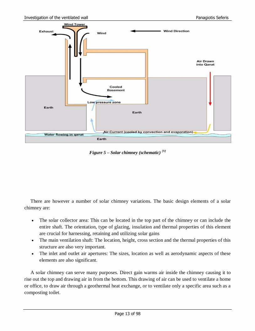
Figure 5 – Solar chimney (schematic) [V]
There are however a number of solar chimney variations. The basic design elements of a solar
chimney are:
The solar collector area: This can be located in the top part of the chimney or can include the
entire shaft. The orientation, type of glazing, insulation and thermal properties of this element
are crucial for harnessing, retaining and utilizing solar gains
The main ventilation shaft: The location, height, cross section and the thermal properties of this
structure are also very important.
The inlet and outlet air apertures: The sizes, location as well as aerodynamic aspects of these
elements are also significant.
A solar chimney can serve many purposes. Direct gain warms air inside the chimney causing it to
rise out the top and drawing air in from the bottom. This drawing of air can be used to ventilate a home
or office, to draw air through a geothermal heat exchange, or to ventilate only a specific area such as a
composting toilet.

Investigation of the ventilated wall Panagiotis Seferis
Page 14 of 98
Natural ventilation can be created by providing vents in the upper level of a building to allow warm
air to rise by convection and escape to the outside. At the same time cooler air can be drawn in through
vents at the lower level. Trees may be planted on that side of the building to provide shade for cooler
outside air.
This natural ventilation process can be augmented by a solar chimney. The chimney has to be
higher than the roof level, and has to be constructed on the wall facing the direction of the sun.
Absorption of heat from the sun can be increased by using a glazed surface on the side facing the sun.
Heat absorbing material can be used on the opposing side. The size of the heat-absorbing surface is
more important than the diameter of the chimney. A large surface area allows for more effective heat
exchange with the air necessary for heating by solar radiation. Heating of the air within the chimney
will enhance convection, and hence airflow through the chimney. Openings of the vents in the
chimney should face away from the direction of the prevailing wind. [5]
Figure 6 – Solar chimney attached to a building
Investigation of the ventilated wall Panagiotis Seferis
Page 15 of 98
1.2 Project objectives and methodology
The purpose of this project is, as its title signifies, the investigation of the ventilated wall. For the
research to cover a larger area of interest there were two kinds of ventilated wall components that were
investigated, the „Typical ventilated wall‟ and the „Upgraded ventilated wall‟. Their difference was the
existence of an additional thin radiant film as a layer in the secondly mentioned wall.
These two kinds of wall are already constructed and tested as part of a test cell under real time
circumstances. All the meteorological (ambient temperature, wind speed, wind direction, relative
humidity, direct and diffuse solar radiation, etc.) and experimental (temperature and wind speed inside
the air zones) data needed were recorded and were suitable for use.
The knowledge of all the appropriate circumstances like the construction details of the test cell and
the meteorological data gave the opportunity to create the simulation model, while the already taken
experimental data offered the option of comparing the simulation with the experimental results.
The modelling of these kinds of ventilated walls helps in the understanding of their functions,
underlining their advantages and disadvantages. This way it can be noted under which circumstances
can they be installed in a larger scale construction and in which kinds of climate they have the best
possible usage.
This thesis tended to be as clear as possible even to somebody that was not informed about the
procedures and natural phenomena that were involved in the ventilated wall. That was why after the
introduction past projects like the double envelope house, the solar chimney and the trombe wall were
mentioned. These projects have some similar functional characteristics with the ventilated wall and are
more familiar to the public.
Next, there is an extensively report on the heat and mass transfer and the air flow procedure in
vertical channels. This report tends to make understood the natural phenomena that are involved in this
project.
After the theoretical part there is the experimental one with the detailed quoting of the test
procedure, the instrumentation that was used, the positioning of each sensor and the codification of the
results.
The creation of the simulation model comes next with the mentioning each step and the showing of
appropriate figure about the model structure and the options that were given by ESP – r, like natural
convection correlations or air flow components choice. Each final choice was partly based on the
theoretical part that was presented before. The setting of this model was based on the meteorological
data that were taken from the experimental part.
Finally, running the simulation model the obtained outcome is compared with the corresponding
experimental. This procedure gives the opportunity to learn more about the simulation model and most
importantly to calibrate it in order to have more accurate results. After that it is going to be more
obvious which can be the benefits regarding the use of different kind of ventilated wall during
different seasons of the year.

Investigation of the ventilated wall Panagiotis Seferis
Page 16 of 98
2. Heat transfer and air flow model
In ventilated walls the heat transfer and the fluid flow are phenomena linked to each other just like
in open air channels. Calculation of outer and inner wall surfaces, convective heat transfer coefficients
and air velocity need to be done at the same time in an integrated way. This chapter contains an
analysis about the heat transfer and the air flow phenomena inside an air channel that will lead, at the
end, to a number of correlations that can be chosen for the convection coefficient of the external and
internal surface of the air gap. The series of equations come from open air channel but with some
further adjustments. The reason of the use of these equations is the similarities between an open
vertical air channel and a ventilated wall regarding the heat and mass transfer processes. These
processes and algorithms are going to be used later on the setting of the simulation model in order for
the results of this model and the experimental ones to be compared.
For the simplification of the analysis, at the beginning, the energy balance equations for each wall
component along with the energy balance of the air flowing in the open channel are going to be
presented.
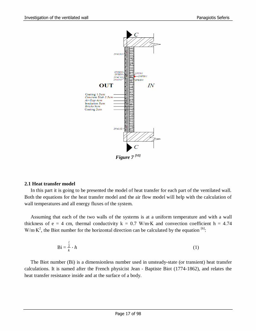
Figure 7 shows a representation of the ventilated wall for modelling purposes. The wall has a
thickness of 24 cm and its structure consisted of:
a 2 cm thickness coating layer in the interior of the room,
a 9 cm thickness brick layer made of 9x6x16 cm bricks,
a 5 cm thickness of rockwood insulation layer in contact with the bricks,
an air gap of 4 cm width,
a 2.5 cm thickness of prefabricated reinforced concrete slab,
a 1.5 cm thickness of mortar on the external, exposed to the environment surface.
Investigation of the ventilated wall Panagiotis Seferis
Page 17 of 98
Figure 7
[VI]
2.1 Heat transfer model
In this part it is going to be presented the model of heat transfer for each part of the ventilated wall.
Both the equations for the heat transfer model and the air flow model will help with the calculation of
wall temperatures and all energy fluxes of the system.
Assuming that each of the two walls of the systems is at a uniform temperature and with a wall
thickness of e = 4 cm, thermal conductivity k = 0.7 W/m∙K and convection coefficient h = 4.74
W/m∙K2, the Biot number for the horizontal direction can be calculated by the equation
[6]:
Bi =
𝑙
2
𝑘∙ (1)
The Biot number (Bi) is a dimensionless number used in unsteady-state (or transient) heat transfer
calculations. It is named after the French physicist Jean - Baptiste Biot (1774-1862), and relates the
heat transfer resistance inside and at the surface of a body.

Investigation of the ventilated wall Panagiotis Seferis
Page 18 of 98
Values of Biot number smaller than 0.1 imply that the heat conduction inside the body is much
faster than the heat conduction away from its surface and temperature gradients are negligible inside of
it. A Biot number less than 0.1 typically indicates less than 5% error will be present when assuming a
lumped-capacitance model of transient heat transfer. [6]
In this case Biot number equals to 0.12. This specific value is slightly higher than 0.1 but
approximately can indicate to neglect the horizontal gradients within each wall component.
On the contrary, in the vertical direction of the system, for a length of 2.75 m the Biot number
becomes 16.5. On this occasion where Biot number‟s value is greater than 0.1 leads to the conclusion
that some vertical temperature gradient may exist if the case of the boundary conditions to which the
wall is exposed vary in the vertical direction as well. The boundary conditions most possibly to vary
vertically are the temperature of the air and the heat convection coefficient in the open air gap and on
the side of the wall that faces indoors.
If the difference in temperature on the vertical axis is less than 2 oC (the temperature on the outlet –
higher spot of the air gap is 2 oC greater than the one on the inlet – lower spot of the air gap), then the
wall can be treated as one with uniform temperature which is the average value of the inlet and outlet
of the air gap.
Figure 8
[VI] – Ventilated wall structure

Investigation of the ventilated wall Panagiotis Seferis
Page 19 of 98
2.1.1 Heat transfer for the outer wall
The exterior wall can exchange energy with the environment by the following ways:
convection with outdoor air,
long wave radiation with the landscape surfaces and the sky,
solar radiation (direct, sky diffuse, ground deflected) absorption,
long wavelength radiation exchange with the inner wall,
convection with the circulating air gap
Additionally it can either store or release heat because of its thermal capacity.
The fluxes for the energy exchange mentioned are:
Convection with outdoor air
hext∙ (Text – T1)
Long wave radiation with the landscape surfaces and the sky
ε1∙(Ilw,out - σ∙T4
1)
Solar radiation (direct, sky diffuse, ground deflected) absorption
α1,dir∙Idirn + α1,dif∙(Idifν + 0.5∙rg∙Gh)
Long wavelength radiation with the inner wall
𝜎 ∙ (𝛵24 − 𝑇1
4)
1𝜀1
+1𝑒2− 1
Convection with the circulating air gap
h1∙ (Tair,mean – T1)
The heat storage of the outer wall in the air gap equals to:
e1∙ρ∙c∙𝜕𝑇1
𝜕𝑡
From the above equations the heat balance for the outer wall is:
hext∙ (Text – T1) + ε1∙(Ilw,out - σ∙T41) + α1,dir∙Idirn + α1,dif∙(Idifν + 0.5∙rg∙Gh) +
𝜎∙(𝛵24−𝑇1
4)1
𝜀1+
1
𝑒2−1
=
h1∙(Tair,mean – T1) (2)

Investigation of the ventilated wall Panagiotis Seferis
Page 20 of 98
2.1.2 Heat transfer for the inner wall
Like the exterior wall with the environment, the interior wall of the air gap can exchange energy
with the room by the following ways:
long wavelength radiation with the outer wall,
long wavelength radiation with the floor and the ceiling of the room,
convection with the air of the room,
convection with the circulating air of the air gap
The interior wall can store or release heat, just like the outer one.
The equations that describe the above assumptions are:
Long wavelength radiation with the outer wall
𝜎 ∙ (𝛵14 − 𝑇2
4)
1𝜀1
+1𝜀2− 1
Long wavelength radiation with room interior surfaces
σ∙ε2∙(Tint4 – T2
4)
Convection with the air of the room
hint∙ (Tint – T2)
Convection with the circulating air of the air gap
h2∙ (Tair,mean – T2)
The heat storage of the inner wall in the air gap equals to:
ε2∙ρ∙c∙𝜕𝑇2
𝜕𝑡
It needs to be mentioned that the temperature of the room internal surfaces, T int, is assumed to be
uniform. In the case where this temperature is known or expected to be significantly different, its
average is used weighted by the area and the view shape factors. For the study of the ventilated wall,
the first approach was used.
The heat balance equation for the inner wall comes from the above individual equations of this
paragraph.
Investigation of the ventilated wall Panagiotis Seferis
Page 21 of 98
𝜎∙(𝛵14−𝑇2
4)1
𝜀1+
1
𝜀2−1
+ σ∙ε2∙ (Tint4 – T2
4) + hint∙ (Tint – T2) + h2∙ (Tair,mean – T2) = ε2∙ρ∙c∙
𝜕𝑇2
𝜕𝑡 (3)
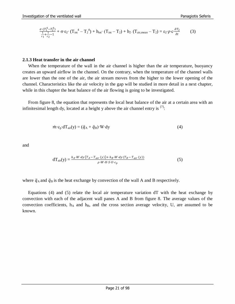
2.1.3 Heat transfer in the air channel
When the temperature of the wall in the air channel is higher than the air temperature, buoyancy
creates an upward airflow in the channel. On the contrary, when the temperature of the channel walls
are lower than the one of the air, the air stream moves from the higher to the lower opening of the
channel. Characteristics like the air velocity in the gap will be studied in more detail in a next chapter,
while in this chapter the heat balance of the air flowing is going to be investigated.
From figure 8, the equation that represents the local heat balance of the air at a certain area with an
infinitesimal length dy, located at a height y above the air channel entry is [7]
:
𝑚 ∙cp∙dTair(y) = (𝑞 A + 𝑞 B)∙W∙dy (4)
and
dTair(y) = 𝐴 ∙𝑊∙𝑑𝑦 𝑇𝐴− 𝑇𝑎𝑖𝑟 𝑦 + 𝐵 ∙𝑊∙𝑑𝑦 (𝑇𝐵− 𝑇𝑎𝑖𝑟 𝑦 )
𝜌∙𝑊∙𝐻∙𝑆∙𝑈∙𝑐𝑝 (5)
where 𝑞 A and 𝑞 B is the heat exchange by convection of the wall A and B respectively.
Equations (4) and (5) relate the local air temperature variation dT with the heat exchange by
convection with each of the adjacent wall panes A and B from figure 8. The average values of the
convection coefficients, hA and hB, and the cross section average velocity, U, are assumed to be
known.

Investigation of the ventilated wall Panagiotis Seferis
Page 22 of 98
Figure 9
Integrating equation (5) from 0 to y, the result is the expression for the temperature at height y [7]
.
Tair (y) = 𝐴 ∙𝑇𝐴+ 𝐵 ∙𝑇𝐵
𝐴+𝐵−
𝐴 ∙ 𝑇𝐴− 𝑇𝐵 + 𝐵 ∙(𝑇𝐵− 𝑇𝑖𝑛 )
𝐴+ 𝐵∙ 𝑒
−𝐴+ 𝐵𝜌 ∙𝑈 ∙𝑆∙𝑐𝑝
∙𝑦 (6)
From equation 6 it is suggested that the equivalent temperature of the channel walls can be defined
as [7]
:
TS = 𝐴 ∙𝑇𝐴+ 𝐵 ∙𝑇𝐵
𝐴+ 𝐵 (7)
Combining equations (6) and (7) the final expression is:
Tair (y) = TS – (TS - Tin) ∙ 𝑒−𝐴+ 𝐵𝜌 ∙𝑈 ∙𝑆∙𝑐𝑝
∙𝑦 (8)
This expression is analogous to the typical one for the evolution of the fluid temperature in an
internal pipe flow.

Investigation of the ventilated wall Panagiotis Seferis
Page 23 of 98
2.1.4 Convection between the external wall and the outdoor air
The fundamental equation used for the prediction of the rate heat transfer is based on the „Newton‟s
law of cooling‟.
𝑞 = hext∙│Ts - Text│
where hext is the convection heat transfer coefficient between the external surface of the wall and the
environment and 𝑞 is the amount of heat per surface unit. The value of hext is dependent on all the
factors that influence the convection transfer process. Parameters like the system geometry, the air
flowing velocity, the specific heat, the viscosity and other physical properties of the air affect the value
of hext.
The analytical approach of the convection heat transfer is difficult because of the large number of
parameters that must be found. This is why simply empirical correlations are used which derive a
relation that combines the pertinent variables, such as the flow velocity and the other air properties,
into dimensionless groups. The most valid relationship between these groups can only be found
experimentally. Also, working by such groups, the number of quantities to be studied is reduced
significantly, the number of experiments is minimised and the interpretation of experimental data is
greatly aided.
As it was mentioned before, there are some variables in the heat transfer equations that need to be
parameterized for known boundary conditions. These variables are the wind speed or temperature and
the wall temperatures. Convection coefficient at the external surface with the outdoor air, convection
coefficients at the air gap and the albedo for the ground reflected solar radiation are parameters that are
affected by the parameters that were mentioned before.
Theoretically, the convection coefficient between the exterior wall and the outdoor air, hext, is the
result of the mix of natural convection caused by the temperature differences and of forced convection
because of the effect of the wind. This is the reason why it depends on conditions like the temperatures
of the walls and of the air, the local wind speed, the wind direction and turbulence. The local geometry
of the wall influences in great deal the local wind speed, direction and turbulence. It is practically
impossible the dynamic prediction through theoretical models. Only CFD analysis can give reliable
results but an analysis like this cannot be performed for all wind conditions throughout all year.
The assumption of a constant value for the external convections coefficient constitutes a simple
solution for overcoming this problem. But this solution can only be used in cases that involve long
term estimations or when information about the wind is not available in climatic data.
The study by McAdams [8]
, of parallel flow in a wind tunnel is another, more realistic approach
since it relies on experiments that take into consideration the effect of wind velocity. In this study, the
convection coefficient is given by the next equation.

Investigation of the ventilated wall Panagiotis Seferis
Page 24 of 98
hext = 5.678∙(α + b∙(𝑉
0.3048)𝑛) (9)
The empirical constants a, b and n in equation (9) depend on two factors: the range of the wind
velocity and the roughness of the wall surface. In table 1, it is presented some typical values of
constants a, b and n for different kind of wall surface and wind velocity. The units of a, b and n are the
appropriate ones in order for dimensional coherence to be assured. In other words, the final output to
be in W/m2∙oC
Table 1
Wind Velocity V < 4.88 m/sec V > 4.88 m/sec
Type of surface a b n a b n
Smooth 0.99 0.21 1 0 0.5 0.78
Rough 1.09 1.23 1 0 0.5 0.78
From table 1 it can be noticed that, when the wind velocity is higher than 4.88 m/s, the type of
surface does not have any effect on the convection coefficient between the wall and the outdoor air.
Something that needs to be mentioned about the McAdams formula is that, although it has been
assumed that the flow is parallel to the exterior wall and the wind velocity in the formula in the one
near the wall, the climatic weather files that are used are typically measured in a tower at 10 m
height without any obstacles.
Ito et al. [9]
adopted another correlation. They managed to interrelate the wind velocity, V, close to
the window with the velocity of the free stream of air, Vf, that was measured in meteorological
stations. This correlation only depends on two factors: the range of the wind speed and if the window
is exposed windward or leeward to the stream of air.
The equations for windward and leeward wind are:
windward wind V = 0.25∙Vf when Vf > 2 m/sec (10)
or V = 0.5 when Vf ≤ 2 m/sec (11)
leeward wind V = 0.3 + 0.05∙Vf (12)
In 1977 Kimura [10]
performed a number of measurements at the 4th floor of a medium – rise
building. Based on these measurements he proposed different formulas associating convection
coefficient between the external wall and the outdoor air and windward or leeward wind.
for windward wind: hext = 6.22 + 1.824∙V (13)
for leeward wind: hext = 6.22 + 0.4864∙V (14)

Investigation of the ventilated wall Panagiotis Seferis
Page 25 of 98
As mentioned before, Kimura‟s outcomes were extracted by measurements at the 4th floor of a
building allowing the rise of concerns about their use in lower height buildings like the one of the
CRES test cell.
On their part, Yazdanian and Klems[11]
(1994) carried out a series of measurements in a low – rise
building this time, conditions that are closer to the CRES test cell. They suggested a correlation that
takes into account the influence of wind as natural convection due to surface – to – air temperature
differences.
For windward wind:
{[0.84∙ │ Ts – Text │1/3
]2 + (2.38∙V
0.89)2}
1/2 (15)
For leeward wind:
{[0.84∙ │ Ts – Text │1/3
]2 + (2.86∙V
0.617)
2}
1/2 (16)
Creating a chart from the above correlations that are mentioned, it can easily be noticed from figure
9 that the prediction of the outdoor convection coefficient can vary a great deal.
For the study of the ventilated wall, the correlation of Yazdanian and Klems is chosen as the
approach. The reason for this choice is because it was made for a low – rise building that most closely
represents the CRES test cell which is the one that was used in the experimental part of the project.
The CRES test cell was 2.75 in length width and height test cell.
Also the fact that for outdoor wind velocities higher than 2 m/s the outdoor convection coefficient
is not affected by the temperature difference allows the study to work on situations with much higher
temperature differences.

Investigation of the ventilated wall Panagiotis Seferis
Page 26 of 98
Figure 10 - Outdoor convection coefficient vs wind speed for different correlations
2.2 Air flow model
The basic variable that describes the balance of forces that act upon the flowing air in the air
channel is the buoyant force. According to Sandberg and Moshfegh [12]
, the definition of the buoyant
force is:
Buoyant force = Force for the fluid to accelerate from rest to the final velocity in the air channel +
Friction force by the surfaces of the air channel + Losses at the entrance + Losses at the exit
Instead of using the above equation, it is equivalent to use the principle of conservation of linear
momentum, where the total momentum of a closed system is constant when it has no interactions with
external agents. As a consequence, the fluid continues with the same velocity unless a force from
outside the system acts on it. This conservation can be used between any point far from the entry of the
channel and the channel exit.
For a valid description of all these terms that were mentioned, the velocity and temperature range of
values not only in the air channels but in the entry and the exit of them is compulsory. This amount of
knowledge is impossible to be acquired. More simplified modelling techniques can be used in order to
have the desirable outcome. These techniques are presented in the next paragraphs.
0
5
10
15
20
25
30
35
40
45
50
1 2 3 4 5 6 7 8 9 10 11
V (
m/s
)
h (W/m2K)
Kimura 4th floor
Yazd. Klems - DT=0
Yazd. Klems - DT=15
McAdams - free velocity
McAdams and Ito et al

Investigation of the ventilated wall Panagiotis Seferis
Page 27 of 98
2.2.1 Buoyant force study
The computation of the Archimedes principle gives an equation that calculates the buoyant force I [13]
.
I = g∙W∙S∙ [𝜌∞ − 𝜌 𝑦 ] ∙ 𝑑𝑦𝐻
0 (17)
The combination of equation (17) with Boussinesq approximation gives equation (18)
ρ ρ∞∙[1 - β∙(T - T∞)] (18)
But for ideal gases the gas expansion coefficient, β = 1
𝑇∞ [7]
Replacing β in equation (18) gives:
I = ρ∞∙g∙W∙S∙ 𝑇 𝑦 − 𝑇∞
𝑇∞∙ 𝑑𝑦
𝐻
0 (19)
2.2.2 Acceleration of fluid
From fluid mechanics, the force needed to be exerted on a fluid in order to obtain a certain velocity
in a channel which is at rest initially equals the dynamic pressure multiplied by the section area [14]
:
Fα = 0.5∙ρ∙W∙S∙U2 (20)
where (W∙S) is the section area and U the final velocity of the fluid in the channel.
2.2.3 Friction force
In order to calculate the friction force of the fluid, the shear stress at the channel walls needs to be
multiplied by the area of the walls [14]
:
Fƒ = 2∙H∙W∙τw (21)
Knowing that the Darcy friction factor equals to [15]
:
ƒ = 8∙𝜏𝑤
𝜌∙𝑈2 (22)

Investigation of the ventilated wall Panagiotis Seferis
Page 28 of 98
The replace of equation (22) in equation (21) results:
Fƒ = 1
4∙ ƒ ∙ 𝐻 ∙ 𝑊 ∙ 𝜌 ∙ 𝑈2 (23)
2.2.3.1 Laminar Flow
From fluid mechanics, for a duct with rectangular section, the value of the friction coefficient for
laminar flow [15]
is:
ƒ = 𝐶
𝑅𝑒𝐷 (24)
The parameter Dh is called hydraulic diameter, is commonly used for the calculation of the flow in
non – circular tubes and channels. Its general definition is [15]
:
Dh = 4∙𝐴
𝛱 (25)
Where A is the cross sectional area and Π is the wetted perimeter of the cross section.
For a rectangular channel equation (25) becomes:
Dh = 4∙𝑊∙𝑆
2∙(𝑊+𝑆) =
2∙𝑊∙𝑆
𝑊+𝑆 (26)
The Reynolds number [14]
taking into account the above equations equals to:
𝑅𝑒𝐷 = 𝜌∙𝑈∙𝐷
𝜇=
𝜌∙𝑈∙2∙𝑊 ∙𝑆
𝑊+𝑆
𝜇 (27)
In equation (24), C represents a constant that depend on the aspect ratio S/W of the air channel. The
value of C can be found by using table 2[16]
and interpolating. Knowing that, for laminar flow in
smooth round ducts, the formula that calculates the friction coefficient is:
ƒ = 64
𝑅𝑒𝐷 (28)

Investigation of the ventilated wall Panagiotis Seferis
Page 29 of 98
makes obvious the fact that there is going to be a slight difference in results.
Table 2
S/W C
0 96.0
0.05 89.9
0.10 84.7
2.2.3.2 Turbulent flow
In order to cover all possible conditions, it has to be assumed that, under certain conditions, the
flow can be turned into turbulent. As in the forced flow, the transition from laminar to turbulent flow
takes place when the value of Reynolds number is greater than 2300. More specifically:
If Re < 2300 then : laminar flow
If 2300 < Re < 4000 then: transient flow
If Re > 4000 then: turbulent flow
The Blausius equation [16]
is commonly used (for Re < 105) to determine the friction coefficient in
round pipes in turbulent flow [16]
.
ƒ = 0.316
𝑅𝑒𝐷0.25 (29)
Unlike for the round pipes, there is no equation that can calculate the friction coefficient in a
rectangular air channel. But, it can be obtained by using equation (29) and multiplying it by an
appropriate correction factor. A possible approximation is using the correction factor obtained from
laminar flow (C/64). The formula that describes this is:
ƒ = 0.316
𝑅𝑒𝐷0.25 ∙
𝐶
64 (30)
2.2.4 Entry and exit losses
Entry and exit losses are taken into account as localised losses. For their calculation the local loss
coefficient K is used.
K = ∆𝑃
1
2∙𝜌∙𝑈2
(31)

Investigation of the ventilated wall Panagiotis Seferis
Page 30 of 98
where ΔΡ is the difference in pressure between two specific spots,
ρ is the density of the fluid and
U is the velocity of the fluid.
For the derivation of K, it is reported that experimental data for a variety of geometries from the
bibliography of fluid dynamics are used. Commonly, it is assumed that the Reynolds number does not
affect the K values. It has to be reminded though, that this assumption can only be made for flows
where the inertial forces are clearly dominant over the viscous ones [16]
. In the case of natural flow and
especially at low Reynolds numbers, an assumption like that cannot always take place.
2.2.5 Force balance implicit equation
At the beginning of the second chapter, the force balance equation was expressed qualitatively. In
this paragraph it is going to be expressed quantitatively.
𝜌 ∙ 𝑔 𝑇 𝑦 − 𝑇𝑖𝑛
𝑇𝑖𝑛∙ 𝑑𝑦 =
1
2 ∙ 𝜌 ∙ 𝑈2 ∙ (1 + ƒ ∙
H
2∙S+ 𝐾𝑖𝑛 + 𝐾𝑜𝑢𝑡 )
𝐻
0 (32)
The typical values for entry (sudden contraction) and exit (sudden expansion) loss coefficients are
Kin = 0.5 and Kout = 1.0 respectively [16]
.
From equation (6), it can be noticed that the profile of the temperature, T(y), along the air channel
and the heat transfer coefficients hA and hB that are presented depend on the velocity of the air. This
dependence makes compulsory the calculation of wall temperatures, heat transfer coefficients and both
the velocity and temperature of the air to be performed in parallel through an iterative procedure until
all the values of the above quantities converge.
2.2.6 Air velocity implicit equation
For the calculation of the velocity of the air in the channel the combination between the right side
of the integral in equation (32) and equation (8) was used. The final formula is:
𝜌 ∙ 𝑔 ∙ 𝑇 𝑦 − 𝑇𝑖𝑛
𝑇𝑖𝑛
𝐻
0
∙ 𝑑𝑦
= 𝜌 ∙ 𝑔 ∙
𝜌∙𝑈∙𝑊∙𝑆∙𝑐𝑝 ∙ 𝑒
𝑊∙𝐻∙(𝐴+𝐵𝜌∙𝑈 ∙𝑊 ∙𝑆∙𝑐𝑝 − 1 + 𝑊∙𝐻∙(𝐴+𝐵 )
𝑊∙(𝐴+ 𝐵 ) ∙
(𝑇𝑠− 𝑇𝑖𝑛 )
𝑇𝑖𝑛 (33)
Since the left side parts of the equations (32) and (33) are the same then their right side are equal.
Investigation of the ventilated wall Panagiotis Seferis
Page 31 of 98
1
2 ∙ 𝜌 ∙ 𝑈2 ∙ 1 + ƒ ∙
H
2 ∙ S+ 𝐾𝑖𝑛 + 𝐾𝑜𝑢𝑡
= 𝜌 ∙ 𝑔 ∙
𝜌∙𝑈∙𝑊∙𝑆∙𝑐𝑝 ∙ 𝑒
−𝑊∙𝐻∙(𝐴+𝐵𝜌 ∙𝑈 ∙𝑊 ∙𝑆∙𝑐𝑝 − 1 + 𝑊∙𝐻∙(𝐴+𝐵)
𝑊∙(𝐴+ 𝐵) ∙
(𝑇𝑠− 𝑇𝑖𝑛 )
𝑇𝑖𝑛 (34)
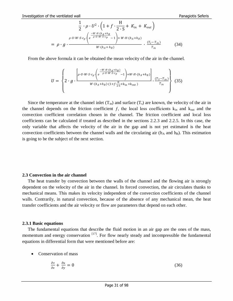
From the above formula it can be obtained the mean velocity of the air in the channel.
𝑈 =
2 ∙ 𝑔 ∙
𝜌∙𝑈∙𝑊∙𝑆∙𝑐𝑝 ∙ 𝑒
−𝑊∙𝐻∙(𝐴+𝐵 )𝜌 ∙𝑈 ∙𝑊 ∙𝑆∙𝑐𝑝 −1 +𝑊∙𝐻∙(𝐴+𝐵 )
𝑊∙ 𝐴+𝐵 ∙(1+ƒ∙H
2∙S+k in +kout )
∙(𝑇𝑆−𝑇𝑖𝑛 )
𝑇𝑖𝑛
(35)
Since the temperature at the channel inlet (Tin) and surface (Ts) are known, the velocity of the air in
the channel depends on the friction coefficient ƒ, the local loss coefficients kin and kout and the
convection coefficient correlation chosen in the channel. The friction coefficient and local loss
coefficients can be calculated if treated as described in the sections 2.2.3 and 2.2.5. In this case, the
only variable that affects the velocity of the air in the gap and is not yet estimated is the heat
convection coefficients between the channel walls and the circulating air (hA and hB). This estimation
is going to be the subject of the next section.
2.3 Convection in the air channel
The heat transfer by convection between the walls of the channel and the flowing air is strongly
dependent on the velocity of the air in the channel. In forced convection, the air circulates thanks to
mechanical means. This makes its velocity independent of the convection coefficients of the channel
walls. Contrarily, in natural convection, because of the absence of any mechanical mean, the heat
transfer coefficients and the air velocity or flow are parameters that depend on each other.
2.3.1 Basic equations
The fundamental equations that describe the fluid motion in an air gap are the ones of the mass,
momentum and energy conservation [17]
. For flow nearly steady and incompressible the fundamental
equations in differential form that were mentioned before are:
Conservation of mass
𝜕𝜈
𝜕𝑥+
𝜕𝑢
𝜕𝑦= 0 (36)

Investigation of the ventilated wall Panagiotis Seferis
Page 32 of 98
Conservation of momentum in the x direction
𝜌 ∙ 𝜈 ∙𝜕𝜈
𝜕𝑥+ 𝑢 ∙
𝜕𝜈
𝜕𝑦 = −
𝜕𝑃
𝜕𝑥+ 𝜇 ∙
𝜕2𝜈
𝜕𝑥2 + 𝜕2𝜈
𝜕𝑦2 (37)
Conservation of momentum in the y direction
𝜌 ∙ 𝜈 ∙𝜕𝑢
𝜕𝑥+ 𝑢 ∙
𝜕𝑢
𝜕𝑦 = −
𝜕𝑃
𝜕𝑦+ 𝜇 ∙
𝜕2𝑢
𝜕𝑥2 + 𝜕2𝑢
𝜕𝑦2 − 𝜌 ∙ 𝑔 (38)
Conservation of energy
𝜈 ∙𝜕𝑇
𝜕𝑥+ 𝑢 ∙
𝜕𝑇
𝜕𝑦= 𝛼 ∙
𝜕2𝑇
𝜕𝑥2 + 𝜕2𝑇
𝜕𝑦2 (39)
The coordinates x and y are defined in the next figure.
Figure 11
Equations (36), (37), (38) and (39) connect the horizontal (u) and vertical (ν) velocities in the air
gap with pressure and temperature. There are only some special conditions for which analytical
solutions could be found [17]
. For these conditions reasonable degrees of decoupling or similarity
analysis can be obtained.

Investigation of the ventilated wall Panagiotis Seferis
Page 33 of 98
The general natural convection flow in a channel is approximately the bounded between two
limiting phenomena:
The natural convection flow along a single vertical plate and
The fully developed channel.
These two phenomena are going to be analyzed in more detail in the next two paragraphs.
2.3.1.1The free vertical plate
In this limiting case, it can be assumed that, when the distance between the two walls of the air gap
(S) is large compared with the height of the channel (H) or when the air velocity is low then the flow
will be similar to the one that is developed along a free vertical surface. Ostrach [18]
and Holman [19]
have already managed to find approximate analytical solutions for this limiting case.
The basic assumption made in order to find these analytical solutions was that the velocity of the
fluid at the edge of the boundary layer is zero. In the case of the ventilated wall the conservation of
mass requires the fluid velocity, even outside of the thermal boundary layer, to be greater zero. It can
be said that an assumption like this is valid only if the aspect ratio H/S is small or if the air flow rates
are very low. Since the second of the conditions can be met, the natural convection along a vertical
plate can be taken as a limiting case of this problem. The next formula [20]
is based on experimental
data, is valid for any value of Rayleigh number and has been used frequently in engineering
applications.
NuL = 0.825 + 0.387 ∙𝑅𝑎𝐿
1/6
1+ 0.492
𝑃𝑟
9/16
8/27
2
(40)
2.3.1.2 The fully developed flow
In order to acquire an analytical solution for the fully developed flow, the equations of paragraph
2.3.1 are used [21]
. Equation (38), for the fully developed flow where ν=0 and 𝜕𝑢
𝜕𝑦= 0 becomes:
0 = − 𝜕𝑃
𝜕𝑦+ 𝜇 ∙
𝜕2𝑢
𝜕𝑥2 − 𝜌 ∙ 𝑔 (41)
Applying the Stevin law of hydrostatic [22]
to the air bordering to the exterior side of the channel the
pressure gradient 𝜕𝑃
𝜕𝑦 is found to be:

Investigation of the ventilated wall Panagiotis Seferis
Page 34 of 98
𝜕𝑃
𝜕𝑦= −𝜌∞ ∙ 𝑔 (42)
Using the Boussinesq approximation, like in a previous paragraph, the local fluid density ρ can be
related with the free fluid density 𝜌∞ through the thermal expansion coefficient β.
𝜌 ≅ 𝜌∞ ∙ 1 − 𝛽 ∙ 𝑇 − 𝑇∞ (43)
Substituting ρ and 𝜕𝑃
𝜕𝑦 in equation (41) results:
0 = − 𝜌∞ ∙ 𝑔 + 𝜇 ∙𝜕2𝑢
𝜕𝑥2− 𝜌∞ ∙ 1 − 𝛽 ∙ 𝑇 − 𝑇∞ ∙ 𝑔 =>
𝜇 ∙𝜕2𝑢
𝜕𝑥2 = −𝛽∙ 𝑇− 𝑇∞
1− 𝛽∙ 𝑇− 𝑇∞ ∙ 𝑔 (44)
If the wall temperatures are moderate, like in the case of the ventilated wall, the quantity
β∙(T - T∞) << 1 and instead of the kinematic v replaces the dynamic viscosity μ. So, equation (44)
finally becomes:
𝜕2𝑢
𝜕𝑥2 = − 𝛽 𝑇− 𝑇∞
𝑣∙ 𝑔 (45)
According to Bejan [21]
, in the fully developed region of the flow the temperature T is nearly equal
to TS, meaning that:
(T - T∞) (TS - T∞) (46)
The above assumption if combined with the boundary condition that at the channel walls the fluid
temperature in the horizontal axis is zero, u = 0, makes the solving of equation (45) easier. It also
obtains the profile of the velocity in the fully developed region.
𝑢 𝑥 = 𝑔∙𝛽∙ 𝑇𝑆− 𝑇∞ ∙𝑆3
8∙𝑣∙ 1 −
𝑥𝑆
2
2
(47)
By the integration of the equation (47) it is possible to estimate the mass flow rate per unit width of
the channel.
𝑚
𝑊= 𝜌 ∙ 𝑢 𝑥 ∙ 𝑑𝑥 =
𝜌∙𝑔∙𝛽 ∙ 𝑇𝑆− 𝑇∞ ∙𝑆3
12∙𝑣
𝑆
0 (48)
Additionally, the energy balance in the air gap between its entry and its exit is [20]
:

Investigation of the ventilated wall Panagiotis Seferis
Page 35 of 98
𝑄
𝑊=
𝑚
𝑊∙ 𝑐𝑝 ∙ 𝑇𝑆 − 𝑇∞ (49)
Alternatively, the transferred heat to the air in the gap equals to [20]
:
𝑄
𝑊= 2 ∙ 𝐻 ∙ ∙ 𝑇𝑆 − 𝑇∞ (50)
The combination of equations (49) and (50) is:
𝑚
𝑊∙ 𝑐𝑝 ∙ 𝑇𝑆 − 𝑇∞ = 2 ∙ 𝐻 ∙ ∙ 𝑇𝑆 − 𝑇∞ (51)
Noting that the heat transfer coefficient between the air and the wall of the channel can be
estimated by the general formula [16]
:
= 𝑁𝑢𝑆 ∙𝑘
𝑆 (52)
It can be obtained an equation that relates the Nusselt number NuS for the walls of the air channel
with heir Rayleigh number RaS and the basic dimensions of the air gap.
𝑁𝑢𝑆 = 𝑅𝑎𝑆 ∙𝑆
24∙𝐻 (53)
The Rayleigh number RaS based on the channel width S equals to:
𝑅𝑎𝑆 = 𝛽∙𝑔∙ 𝑇𝑆− 𝑇∞
𝑣∙𝛼 (54)
2.3.2 Combined correlations
In paragraphs 2.3.1.1 and 2.3.1.2 there were presented two correlations for the calculation of the
heat transfer between the air and the walls in a channel. These two correlations represented two
different cases for the flow in an air gap: the single plate and the fully developed channel flow.
The reason for the choice of these two limiting cases is the fact that the flow in an air channel lays
between them. When the flow rate or the aspect ratio H/S is low the heat transfer from convection
behaves closer to the single plate. Contrarily, when the flow rate or the aspect ratio is high the
convection heat transfer is expected to behave like in the case of the fully developed flow.

Investigation of the ventilated wall Panagiotis Seferis
Page 36 of 98
There were various proposals for a general methodology that would combine the already mentioned
two limiting cases. One of them by Churchill and Usagi [23]
has the following general form:
𝑁𝑢 = 1
𝑁𝑢𝑠𝑝 𝑛
+ 1
𝑁𝑢𝑓𝑑 𝑛
−
1
𝑛
(55)
where Nusp and Nufd are the Nusselt number calculated for the case of the single plate and the fully
developed flow respectively.
Based on this general formula there were plenty of propositions about the blending constant n.
Churchill and Usagi proposed that n = 1.5. On the other hand the proposition by Bar – Cohen and
Rohsenow [24]
was for a blending constant of n = 2. It has to be mentioned that this methodology was
applied in the investigation of the cooling in a variety of electronic devices and the optimal spacing
between vertical plates.
Churchill and Usagi correlation
𝑁𝑢 = 1
𝑁𝑢𝑠𝑝
1.5
+ 1
𝑁𝑢𝑓𝑑
1.5
−1
1.5
(56)
Bar – Cohen and Rohsenow correlation
𝑁𝑢 = 1
𝑁𝑢𝑠𝑝
2
+ 1
𝑁𝑢𝑓𝑑
2
−1
2
(57)
Another correlation that is used both for a vertical channel with isothermal walls is of Incropera and
DeWitt [6]
and for a vertical channel with only one of the facing walls heated (Sparrow and Azevedo
[25]) is:
𝑁𝑢𝑆 = 5.76 ∙ 𝑅𝑎𝑆𝑆
𝐻 −2
+ 2.87 ∙ 𝑆
𝐻 −
1
2
−1
2
(58)

Investigation of the ventilated wall Panagiotis Seferis
Page 37 of 98
2.3.3 Comparison of correlations
The use of equations 40, 53, 56 and 57 led to the creation of figure 12, which shows the Nusselt
number as a function of the modified Rayleigh number. This last mentioned parameter comes from the
multiplication of the Rayleigh number by the aspect ratio of the air channel (S/H).
As expected, the results that come from the blending of Churchill and Usagi (n=1.5) are quite
similar to those of the Bar – Cohen and Rohsenow blending (n=2). Also these two correlations give
results close to the ones of the fully developed flow when the aspect ratio 𝑆
𝐻 → 0 and close to the ones
of the single plate when 𝑆
𝐻 → ∞.
Figure 12 – Nusselt number vs. modified Rayleigh number for a channel of 4 cm width and 1.375 m height
-10
0
10
20
30
40
50
60
70
-200 0 200 400 600 800 1000 1200 1400 1600
Nu
s
Ras*(S/H)
Single plate
Fully developed flow
Churchill and Usagi, n=1.5
Bar-Cohen and Rohsenow, n=2

Investigation of the ventilated wall Panagiotis Seferis
Page 38 of 98
3. Experimental setup
3.1 Introduction
For the experimental part of this study, the experimental data obtained from tests of a ventilated
wall in the frame of the AIRinSTRUCT project were used. A prototype of the PROKELYFOS
ventilated wall component was constructed in the frame of the AIRinSTRUCT project in order for a
series of tests to be carried out. This test component consisted of a prototype wall component that was
built in one to one scale and tested under real outdoor weather conditions. [27, 28]
The objectives of the experiments of the wall component were:
Collection of information about the wall component operational characteristics in order for its
specific aspects of design and operation to be understood in the greatest deal possible.
Investigation of the thermal performance of the ventilated wall component during the heating
and the cooling period.
Deeper understanding and classification of the effects of different parameters such as:
- the inlet and outlet opening area of the ventilation gap
- the radiant barrier the was installed at the ventilation gap
- the air flow mode (natural convection)
Validation of the simulation model that was created for this project.
The wall component consisted of two different ventilated wall parts. These parts have the same area
but different characteristics. The measurements at both of these wall parts were simultaneously carried
out in order to achieve a comparative study about the performance on the two components. They were
both installed at the south side of the test cell and covering, each one of them, half of the total wall
area. The separation of them was achieved by an insulation layer. [27, 28]
The PASSYS Test Cell that the experiments were carried out was located at the CRES (Centre of
Renewable Energy Sources) site, at Pikermi. The specific place is just outside Athens which has a
latitude of 37o 58‟ N, a longitude of 23
o 42‟ E and is placed at an altitude of 130m. The installation of
the wall component was on the Mediterranean PASSYS test cell. This cell had a removable south wall
and a roof equipped with a Pseudo – Adiabatic Shell (PAS). [27, 28]

Investigation of the ventilated wall Panagiotis Seferis
Page 39 of 98
3.2 Description of the wall component
The experimental wall component was created by the manufacturing company PROKELYFOS
S.A. For the construction of the wall components the design and the technical specifications of the
prefabricated building were followed by the above company. The wall, which has a length and a height
of 2.75m each, was split into two equal areas.
Half of the wall was constructed as the PROKELYFOS ventilated wall component and was
called ‘Typical wall’ and
The other half was constructed as the PROKELYFOS ventilated wall component with and
additional layer of radiant barrier installed in its internal surface of the prefabricated external
concrete slab. This part of the ventilated wall was called ‘Upgraded Ventilated wall’.
Each equal half of the wall covers the same area of 3.69m2. Figure 12 shows the overall dimensions
of the south facing wall which is separated into the two different wall components. [27, 28]
Figure13
[VI] - Total dimensions of ventilated wall – Sensors position

Investigation of the ventilated wall Panagiotis Seferis
Page 40 of 98
3.2.1 Composition of the wall component
Typical wall
The Typical PROKELYFOS ventilated wall covered half of the test cell‟s south wall and its
structure consisted of:
Plaster, in the interior of the room, with a thickness of 2 cm,
a brick layer made of 9x6x19 cm bricks with a total thickness of 9 cm,
a rockwool insulation layer of 5 cm that is in contact with the brick layer,
an air gap with a width of 4 cm,
a 2.5 cm thickness of prefabricated, reinforced concrete slab and,
a 1.5 cm thickness of mortar placed on the external surface of the wall.
The width and height of the „Typical wall‟ are 1.375m and 2.75m respectively. Adding the
thickness each layer and air gap that are mentioned before gives a total wall thickness of 24cm. [27, 28]
Figure 14
[VI] - Typical wall cross section – Sensors position

Investigation of the ventilated wall Panagiotis Seferis
Page 41 of 98
Upgraded Ventilated wall
The composition of this wall part is:
a 2 cm thickness plaster in the interior of the room,
a 9 cm thickness brick layer made of 9 x 6 x 19 cm bricks,
a 5 cm thickness of rockwool insulation layer in contact with the bricks,
an air gap of 4 cm width,
a radiant barrier in contact with the reinforced, prefabricated concrete slab,
a 2.5 cm thickness of prefabricated, reinforced concrete slab and
a 1.5 cm thickness of mortar on the external surface of the wall
Like the „Typical wall‟, the dimensions of the „Upgraded Ventilated wall‟ are the same, 2.75m to
1.375m of height and width. The total wall thickness can also be taken as 24cm since the radiant
barrier that was added has a thickness of 0.1mm, which is negligible. [27, 28]
Figure 15
[VI] - Upgraded Ventilated wall cross section – Sensors position

Investigation of the ventilated wall Panagiotis Seferis
Page 42 of 98
3.2.2 Phases of the Ventilated wall construction
The wall component that was tested was placed inside an insulated frame which was made of
polystyrene insulation and plywood layers. The reason for the design and construction of this frame
was the prevention of thermal edge effects and the promotion of one - dimensional heat transfer
through the wall test components. Frames like this can be used for the testing of wall components of
up to 40 cm.
The steps for the construction of the ventilated wall were:
1. In order to avoid heat transfer between the walls, each wall part, at the beginning, was
constructed singularly on the insulation frame and was separated with an 8 cm thick insulation
layer (extruded polystyrene). (Figures 16, 17)
Figure 16
[VI] – Construction of the brick layer

Investigation of the ventilated wall Panagiotis Seferis
Page 43 of 98
Figure 17
[VI] - Positioning of the special metal support elements for the fixing of the prefabricated
concrete slab
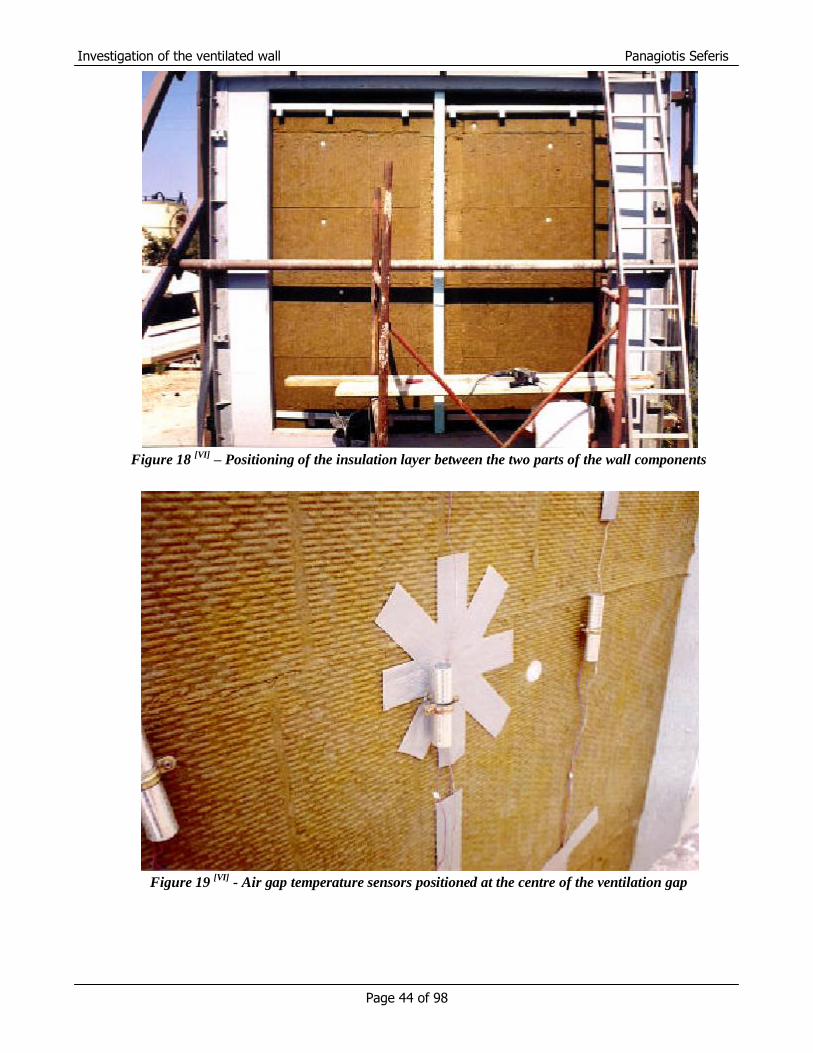
2. In order to ensure the constant and specific air gap thickness (4 cm), special metal support
elements were used. This elements were designed and manufactured by the PROKELYFOS
S.A and were positioned at the top and the bottom of each brick wall part. This way, the
external prefabricating slab was successfully supported in the prefixed distance from the brick
wall (Figures 18 and 19)
3. The insulation layer of the wall was placed in contact with the brick layer by using thin plastic
bolts and screwing them into the brick layer (Figure 18)
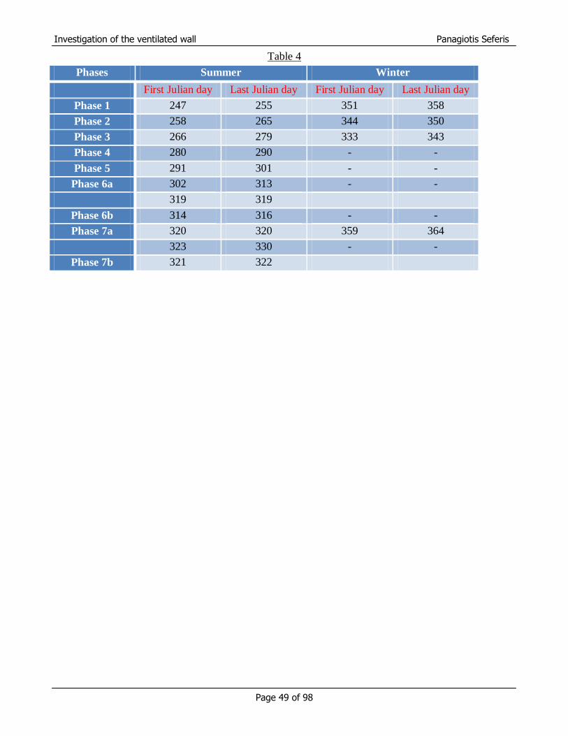
4. For the measurement of the air gap temperature distribution, 9 temperature sensors were
positioned in each the ventilation gap. For the elimination of the radiation effects that take
place between the two opposite internal surfaces, these sensors were shielded.
Investigation of the ventilated wall Panagiotis Seferis
Page 44 of 98
Figure 18
[VI] – Positioning of the insulation layer between the two parts of the wall components
Figure 19
[VI] - Air gap temperature sensors positioned at the centre of the ventilation gap

Investigation of the ventilated wall Panagiotis Seferis
Page 45 of 98
5. The external layer of the ventilated wall was made by a metallic mesh, paperboard and a
concrete layer of 2.5 cm thickness (Figure 20). The metal mess was used to reinforce the
concrete slab while the paperboard was added in order to protect the air temperature sensors
that were placed along the air gap. At the backside of the external layer of the „Upgraded
Ventilated wall‟, a sheet of radiant barrier was positioned. The ventilated wall‟s external layer
was fixed at the metal support elements that were placed on the brick wall part.
6. The air openings were created as rectangular openings of 15 cm length and 2 cm height. There
were 6 openings on each wall, three of them placed at the very bottom and the other three at the
very top of the external concrete slab. Having the option of having some of them open or
closed gives the capability to change the flow rate inside the air gap.
Figure 20
[VI] – Construction of the external concrete slab - view of the air gap temperature sensors

Investigation of the ventilated wall Panagiotis Seferis
Page 46 of 98
Figure 21
[VI] – Positioning of the wall component in the test cell – view of the meteorological mast
7. Both the interior and exterior sides of the wall consist of mortar layers of 1.5 cm and 2cm
thickness respectively. On these layers (interior and exterior surfaces), a series of temperature
sensors were also positioned.
8. In the „Typical wall‟ part a small hole of 2cm diameter was drilled in order for the air velocity
sensor to be positioned.(Figure 22)
9. For the whole construction made to dry out, the concrete slab remained unmoved for a period
of 10 days after its completion. After it was dried out, it was moved by a crane and placed on
the south side of the test cell.

Investigation of the ventilated wall Panagiotis Seferis
Page 47 of 98
Figure 21
[VI] – Final set up of the test cell
Facing the danger of the creation of thermal bridges between the wall components and in order to
ensure air tightness extra attention was given. At the internal perimeter of the wall joints with the
insulated frame special insulating tapes were placed.

Investigation of the ventilated wall Panagiotis Seferis
Page 48 of 98
3.3 Experimental procedure
During the experimental procedure simultaneous reading had been taken for both the „Typical
Ventilated wall‟ and the „Upgraded Ventilated wall‟. In both cases the air gap thickness had the
constant thickness of 4 cm. Each experimental layout was called „Phase‟. There were 9 „Phases‟ and
they were designed so that different parameters of the ventilated wall components to be investigated.
These parameters were:
The inlet and outlet area of the ventilation gap
The mode of the air flow inside the air gap (natural or forced convection)
The control scheme of the applied indoor temperature
A summary of the conditions of each Phase is presented in the next table
Table 3
Open slot
Inlet/Outlet
Flow Mode Control Scheme
Phase 1 1/1 Natural Flow Constant Indoor Temperature
Phase 2 2/2 Natural Flow Constant Indoor Temperature
Phase 3 3/3 Natural Flow Constant Indoor Temperature
Phase 4 2/3 Forced Ventilation 0.5 m/s Constant Indoor Temperature
Phase 5 3/3 Forced Ventilation 1.4 m/s Constant Indoor Temperature
Phase 6a 3/3 Forced Ventilation 1.4 m/s Constant Heating Power 150W
Phase 6b 3/3 Forced Ventilation 1.4 m/s Constant Heating Power 80W
Phase 7a 3/3 Natural Flow Constant Heating Power 150W
Phase 7b 3/3 Natural Flow Constant Heating Power 80W
- In Phase 6a the constant heating power of 150W is taken approximately equal to the
internal gains in the testroom.
- In Phase 6b the constant heating of 80W corresponds to the fan power used for the
circulation of air inside the testroom.
The constant indoor temperature as a control scheme is translated into a constant temperature of 27 oC ± 0.2
oC.
In order to have more representative data for the wall component behaviour the experiments took
place during two separate periods (winter and summer season). During the summer season all night
phases were extensively tested. On the contrary, during the winter season, only 4 phases were tested
(Phase 1, Phase 2, Phase 3 and Phase 7a). The reason for that was the fact that the remaining phases‟
flow mode was with forced convection, something that would have negative effects on the ventilated
wall‟s performance. The periods of each experimental phase are shown on the next table. [27]
Investigation of the ventilated wall Panagiotis Seferis
Page 49 of 98
Table 4
Phases Summer Winter
First Julian day Last Julian day First Julian day Last Julian day
Phase 1 247 255 351 358
Phase 2 258 265 344 350
Phase 3 266 279 333 343
Phase 4 280 290 - -
Phase 5 291 301 - -
Phase 6a 302 313 - -
319 319
Phase 6b 314 316 - -
Phase 7a 320 320 359 364
323 330 - -
Phase 7b 321 322

Investigation of the ventilated wall Panagiotis Seferis
Page 50 of 98
3.4 Instrumentation
For the monitoring of the thermal performance of the Test Cell, the standard PASLINK
instrumentation of the Test Site and was used. The environmental parameters that were also measured
were:
the ambient temperature,
the relative humidity,
the wind speed,
the wind direction,
the horizontal radiation,
the vertical radiation and
the diffuse solar radiation
Also, the sky long – wave radiation was monitored with the use of a Pyrgometer. There was a
number of sensors that were installed for the performance of the wall component to be measured.
Sensors of the wall component
The location and the names of the sensors used for this series of tests are shown in figures 1, 2, 3
and 11 and were placed:
In the Prefabricated reinforced concrete slab: 1 T – type thermocouple on the external surface
of each wall part. These thermocouples were firmly attached with two layers of tape, one of
them thermally insulated, covered with an external reflective tape.
In the air gap: 9 T – type thermocouples for the measurement of air temperature in the
ventilation air gap, in the middle of the width of the air gap of each wall part.
In the air gap: 1 low velocity, hot wire anemometer for the measurement of the air velocity in
the middle of the air gap of the „Typical Ventilated wall‟.
In the insulation layer, brick layer and mortar: 1 T – type thermocouple for the measurement
of the temperature on the external surface of each wall part.
On the plaster of the wall component: 2 heat flux meters installed on each wall part.
All the acquired data from the sensors were collected at the Test Cells accompanied Data
Acquisition System (DAS). [27]

Investigation of the ventilated wall Panagiotis Seferis
Page 51 of 98
3.4.1 Position of the wall component sensors
In the following table there are presented in detail not only the names of the sensors but also their
position on the wall component. [27]
Table 5
Sensor name Location Position Units
Typical wall Upgraded
wall
2PSE01 2FSE01 Prefabricated slab
surface external
temperature
Centre 2/3 height (oC)
2PISE01 2FISE01 Insulation external
surface
temperature
Centre 2/3 height (oC)
2PBE01 2FBE01 Brick layer external
surface
temperature
Centre 2/3 height (oC)
2PTI01 2FTI01 Plaster, internal
surface
temperature
Centre 2/3 height (oC)
2PAU01 2FAU01 Air gap
temperature
¼ width 15 cm from
top
(oC)
2PAU02 2FAU02 Air gap
temperature
½ width 15 cm from
top
(oC)
2PAU01 2FAU01 Air gap
temperature
¾ width 15 cm from
top
(oC)
2PAC01 2FAC01 Air gap
temperature
¼ width 2/3 height (oC)
2PAC02 2FAC02 Air gap
temperature
½ width 2/3 height (oC)
2PAC03 2FAC03 Air gap
temperature
¾ width 2/3 height (oC)
2PAL01 2FAL01 Air gap
temperature
¼ width 15 cm from
top
(oC)
2PAL02 2FAL02 Air gap
temperature
½ width 15 cm from
top
(oC)
2PAL03 2FAL03 Air gap
temperature
¾ width 15 cm from
top
(oC)
2PAV01 - Air velocity at the
air gap
Centre 2/3 height (m/s)
2HFS01 2HFS02 Heat flux sensor Plaster 2/3 height (oC)

Investigation of the ventilated wall Panagiotis Seferis
Page 52 of 98
3.4.2 Test cell sensors
The naming and position of the Standard PASLINK sensors that were used during the tests to
monitor the indoor environment of the Test Cell are:
2HPI01 : heating power of the heating resistances (W)
2HPI02 : heating consumed by the fan system (W)
2WFI01 : water flow of the cooling system (l/min)
2ATI01 : internal air temp., centre of floor, 15cm height (oC)
2ATI02 : internal air temp., centre of ceiling, 15cm below (oC)
2ATI03 : internal air temp., centre of east wall, 15cm off (oC)
2ATI04 : internal air temp., centre of west wall, 15cm off (oC)
2ATI05 : internal air temp., centre of test room (oC)
2ATI06 : internal air temp., centre of partition wall, 60cm off (oC)
2ATI07 : internal air temp., centre of calibration wall, 60cm off (oC)
2SFTAV : internal mean air temperature, software channel (oC)
2RTI01 : dry resultant temp. in centre of service room (oC)
3.4.3 Environmental sensors
The description and position of the Standard PASLINK environmental sensor are:
0ATE01 : Ambient air temperature, 2m height to south of cells (oC)
0GVE01 : Global vertical solar radiation, 2m height to south of cells (W/m2)
0GHE01 : Global horizontal radiation, test cell roof (W/m2)
0DHE01 : Diffuse horizontal radiation, test cell roof (W/m2)
0RHE01 : Relative humidity, 10m height (%)
0AVE01 : Wind speed, 10m height (m/s)
0ADE01 : Wind direction, 10m height (degrees)
0IRE01 : Sky longwave radiation (W/m2)

Investigation of the ventilated wall Panagiotis Seferis
Page 53 of 98
Figure 22 [VI]
Investigation of the ventilated wall Panagiotis Seferis
Page 54 of 98
4. Simulation model
4.1 The ESP – r simulation software
For the creation of the simulation model of this project the ESP – r (Environmental Systems
Performance research version) energy simulation environment was chosen [26]
. The main reasons that
led to this decision were:
It has a specific orientation concerning its abilities in research. The purpose of simulating the
real world is dictated by international research efforts and results. It only uses generally
applicable techniques meaning that for a specific technique there must be a certain amount of
international consensus in its use.
It takes into account all building and plant energy flows and their interconnections. It also
connects building and plant performance with the resulting thermal comfort. This function
makes ESP – r suitable for researches in which energy and mass flow play an important role.
It is free in its use. Its installer file can be downloaded by the website
http://www.esru.strath.ac.uk.
It is well documented having notices that can be used during its use or in the case of a detailed
written user manual which is renewed on regular basis.
Various international research groups use ESP – r contributing to the improvement of its
various functions by giving helpful notices from real case studies.
This software still remains until the present day a subject of a number of international
validation programmes.
It offers a well build graphic environment.
Even if ESP – r was built in the UNIX code environment, the last years, it runs on windows
environment as well. That makes it much more accessible to anybody that just uses an ordinary
PC.
4.2 Creation process
In order for the results of the upcoming simulation to be compared with the experimental ones, the
simulation model, which was constructed in ESP –,r was completely based on the PROKELYFOS test
cell.
After discussion with the supervisors of the project, it was decided that the simulation model would
be created based on the setting of „Phase 3‟ of the experimental series. The reason of this decision was
that it was much more interesting, even though it is generally more complex the investigation of the
natural flow inside the air gap and the fact that there were climate data taken for both winter and
summer period. All the above would have led to more sufficient outcomes.

Investigation of the ventilated wall Panagiotis Seferis
Page 55 of 98
For this „Phase‟ all the air gap openings (3 inlet and 3 outlet) were open. Also, as mentioned in the
above paragraph, the air inside the facade circulated by natural means mostly because of the difference
in temperature and pressure between the inlet and outlet openings. Finally, for both periods the
temperature inside the testroom was kept constant at 27 oC.
Climate data
The file of the climate data was provided by members of staff that took part in the experiment and it
contained measurements of the basic weather parameters which were taken during the test period.
These parameters were the ambient temperature (oC), diffuse solar radiation (W/m
2), direct solar
radiation (W/m2), wind velocity (m/s), wind direction and relative humidity (%). The measurements
were taken every 10 minutes from the 266th to the 279
th Julian day (summer period) and from the
333th to the 343th Julian day (winter period).
Materials
The next step was the creation of the materials which the „Typical ventilated wall‟ and the
„Upgraded Ventilated wall‟ consisted of. These materials and their basic properties are shown in the
next table.
Table 5
Density
(kg/m3)
Thickness
(m)
Conductivity
(W/m∙oC)
Mortar 1900 0.015 0.870
Plaster 1900 0.02 0.870
Rockwool 40 0.05 0.035
Brick layer 1000 0.09 0.460
Concrete slab* 1950 0.025 1.060
*in the case of the „Upgraded Ventilated wall‟ the emissivity of the concrete slab was considered to be
0.20 instead of 0.90 of the „Typical Ventilated wall‟ because of the radiant barrier that was added on
its surface.
Constructions
For reasons that will be explained in a following paragraph, each one of the „Typical Ventilated
wall‟ and the „Upgraded Ventilated wall‟ were divided into two individual walls. This way the „wall
1‟, „wall 2‟ and „wall 2 with radiant‟ were created. Their composition, starting from the outer layer,
was:

Investigation of the ventilated wall Panagiotis Seferis
Page 56 of 98
Vent. Wall 1
Coating with 0.02 m thickness.
Brick layer with 0.09 m thickness.
Rockwool insulation with 0.05 m thickness
Vent. Wall 2
Coating with 0.015 m thickness.
Prefabricated concrete block with 0.09 m thickness.
Vent. wall 2 with radiant barrier
Coating with 0.015 m thickness.
Prefabricated concrete block with 0.09 m thickness and low emissivity of 0.2.
Finally, the rest of the walls of the testroom were characterized as „simple vent. wall‟ with
composition of:
Coating with 0.015 m thickness.
Prefabricated concrete block with 0.09 m thickness.
Rockwool insulation with 0.05 m thickness
Brick layer with 0.09 m thickness.
Coating with 0.02 m thickness.
Zones
It can be said that this was actually the part where the research of the projects begins. Up until then,
all the steps that needed to be done were a straight forward act. The creation of the air zones required a
deeper understanding of the nature of the project. All the natural processes that were involved, like
natural and forced convection, conduction, radiation, fluid flow variations etc., had to be taken into
account so that the model was as accurate as possible and to reduce differences between model
predictions and measurements.
Primarily, three air zones were created:
1. the facade 1 air zone
2. the facade 2 air zone and
3. the testroom air zone
The facade 1 air zone and the facade 2 air zone represented the 4 cm air gap in the „Typical
Ventilated wall‟ and the „Upgraded Ventilated wall respectively while the testroom air zone, as its
name indicates, represented the air zone in the test cell.

Investigation of the ventilated wall Panagiotis Seferis
Page 57 of 98
In the next figures they are presented the entire simulation model and the facade 1 individually as
they were constructed in the ESP – r environment.
Figure 23 – Simulation model in ESP - r
Figure 24 – Facade 1

Investigation of the ventilated wall Panagiotis Seferis
Page 58 of 98
The testroom was 2.75x2.75x2.75 m in length, width and height. Each facade, on the other hand,
had a length of 1.35m, width of 0.04m and height of 2.75m.
This first stage of the construction of the ESP – r model established the basic principles on which
the project would be based on and designated its continuance and evolution.
Figure 25
The final adjustment regarding the air zones was the separation of each air facade into three parts in
order to take into account of temperature stratification. The shape and dimensions of the air channel
zones are represented in figure 25. The separation of the two initial air zones made the model‟s results
more accurate since the air zones were of smaller volume. With three zones on each side of the wall
there were more options provided in the investigation of the air channel. Along with the previous
change in the air facade zones, the testroom had to be altered in order to accomplish the appropriate
correspondence between the opposite surfaces (Figure 26).

Investigation of the ventilated wall Panagiotis Seferis
Page 59 of 98
Figure 26 – Final shape of the testroom
The surface attribute of each air zone are analytically presented in the next tables. Figures 26 and
27 indicate the naming of the surfaces in the testroom and each air zone of the facades.
Figure 27 – Facade 1b

Investigation of the ventilated wall Panagiotis Seferis
Page 60 of 98
Table 6 – Facade 1a
Name Composition Facing
Wall 1 Vent. Wall 2 Exterior environment
Wall 2 Insulation material Adiabatic*
Wall 3 Vent. Wall 1 Another zone
Wall 4 Simple vent. wall Adiabatic**
Base Simple vent. wall Adiabatic
Top Fictitious Another zone
Table 7 – Facade 1b
Name Composition Facing
Wall 1 Vent. Wall 2 Exterior environment
Wall 2 Insulation material Adiabatic*
Wall 3 Vent. Wall 1 Another zone
Wall 4 Simple vent. wall Adiabatic**
Base Fictitious Another zone
Top Fictitious Another zone
Table 8 – Facade 1c
Name Composition Facing
Wall 1 Vent. Wall 2 Exterior environment
Wall 2 Insulation material Adiabatic*
Wall 3 Vent. Wall 1 Another zone
Wall 4 Simple vent. wall Adiabatic**
Base Fictitious Another zone
Top Fictitious Another zone
Table 9 – Facade 2a
Name Composition Facing
Wall 1 Vent. Wall 2 with rad. barrier Exterior environment
Wall 2 Simple vent. wall Adiabatic**
Wall 3 Vent. Wall 1 Another zone
Wall 4 Insulation layer Adiabatic*
Base Simple vent. wall Another zone
Top Fictitious Adiabatic

Investigation of the ventilated wall Panagiotis Seferis
Page 61 of 98
Table 10 – Facade 2b
Name Composition Facing
Wall 1 Vent. Wall 2 with rad. barrier Exterior environment
Wall 2 Simple vent. wall Adiabatic**
Wall 3 Vent. Wall 1 Another zone
Wall 4 Insulation layer Adiabatic*
Base Fictitious Another zone
Top Fictitious Another zone
Table 11 – Facade 2c
Name Composition Facing
Wall 1 Vent. Wall 2 with rad. barrier Exterior environment
Wall 2 Simple vent. wall Adiabatic**
Wall 3 Vent. Wall 1 Another zone
Wall 4 Insulation layer Adiabatic*
Base Fictitious Adiabatic
Top Simple vent. wall Another zone
Table 12 – Testroom
Name Composition Facing
Wall 1 Vent. Wall 1 inv.*** Another zone
Wall 2 Simple vent. wall Exterior environment
Wall 3 Simple vent. wall Exterior environment
Wall 4 Simple vent. wall Exterior environment
Top Simple vent. wall Exterior environment
Base Simple vent. wall Exterior environment
Wall 7 Vent. Wall 1 inv*** Another zone
Wall 8 Vent. Wall 1 inv*** Another zone
Wall 9 Vent. Wall 1 inv*** Another zone
Wall 10 Vent. Wall 1 inv*** Another zone
Wall 11 Vent. Wall 1 inv*** Another zone

Investigation of the ventilated wall Panagiotis Seferis
Page 62 of 98
*It was initially set that between the ventilation gaps there was no heat exchange. This is why it is set
to „adiabatic‟ instead of „another zone‟.
**Because of the insignificant side area of the facades, the heat exchange between them and the
environment can be set to 0. On this occasion the facing column is set to „adiabatic‟ instead of
„external environment‟.
***On respect of the testroom, the wall that separates its surfaces and the ones of the air facades is the
„Ventilated wall 1‟ but inverted. This wall was entirely created by ESR – r itself during the process.
Convection coefficients
After the air zones were created and their surface attributes were set, it had to be investigated the
way of thermal exchange, because of the convection process, between the circulating air in the facades
and the inner surfaces of the walls.
Figure 26 – Convection correlations types
[30]

Investigation of the ventilated wall Panagiotis Seferis
Page 63 of 98
ESP – r comprises a number of different kinds of convection correlations that can be chosen
depending on a variety of parameters. The main characteristic that separates these correlations into
subcategories is the driven flow of the fluid (air or water). As figure 26 indicates, the user can choose
between a buoyancy, mechanically or a mixed (buoyancy and mechanically) driven flow. He (or she)
can also set a user defined values of the convective regime if the above choices do not correspond to
the nature of the fluid flow.
Options a-c are appropriate when convection in the zone is driven primarily by buoyancy resulting
from surface- to-air temperature differences caused by in-floor heating, a heated wall panel, sun-patch
or cold window.
Options d-e are appropriate when convection is driven primarily by buoyancy resulting from a
heating device (e.g. radiator, stove) located either under a window or at some other location in the
zone.
Options f-g are specific for treating convection inside open vertical channels with buoyancy driven
flow.
Options h-j are appropriate when convection is driven primarily by an air-handling system that
supplies heated or cooled air to the zone through ceiling floor or wall-mounted diffusers. It should not
be used when buoyancy is also a significant factor.
Option k is appropriate when convection in the zone is driven primarily by a heating or cooling
device that circulates air within the zone. There is no intentional supply or extract of air from the zone.
Options l-m are appropriate when convection in the zone is driven by both mechanical and buoyant
forces. The mechanical forces are caused by an air handling system (AHU) that supplies heated or
cooled air to the zone through ceiling, floor, or wall-mounted diffusers. The buoyant forces are caused
by surface-to-air temperature differences. This option is preferred over the `air-based HVAC system`
convective regime as it captures the combined influence of buoyant and forced effects.
The correlation that was chosen was the Bar – Cohen and Rosenhow correlation which was
generically developed for open vertical channels and was extensively mentioned in the theoretical part
of this project. This procedure was independently done for every air facade zone with a common
channel width of 0.04m and height that varies as it is shown in figure 24. No correlation was chosen
for the testroom air zone since it was not necessary (it was set as undefined).

Investigation of the ventilated wall Panagiotis Seferis
Page 64 of 98
Fluid flow network
In order for the fluid flow problem to be applied to the simulation system, the fluid flow network
has to be defined first. The nodes of the fluid network may represent rooms, connection points in a
duct or in a pipe network, the outdoor environment, etc. On the other hand, fluid flow components
correspond to discrete fluid flow passages like doorways, construction cracks, ducts, pipes, fans,
pumps, etc.
Node data
Nodes are characterised by a name/identifier, fluid type, node type, height above datum,
temperature, and up to two supplementary data items. ESP – r until now supports only two types of
fluid: air and water. At present only two fluid types are supported: air and water. The possibilities with
respect to node type are summarized in figure 27.
Figure 27 – Node types
[30]
The nodes of the network represent either internal or boundary pressures. The difference is that
only internal nodes are subjected to the mass balance approach. It has to be noted that ‟internal‟ is not
necessary equivalent to ‟inside‟ nor does ‟boundary‟ need to be equivalent to ‟outside‟. Usually the
pressure at an internal node is unknown.
The setting of the nodes concerning their position in the air facade zones was the same with the
temperature sensors in the experimental model. The height above the lower surface of the wall was
0.15 m, 1.83 m, and 2.60 for both sides of the wall (Figures 29 and 30). The lower external node was
placed 0.5 m lower of the base datum while the upper external node was 0.25 m above the roof
surface.

Investigation of the ventilated wall Panagiotis Seferis
Page 65 of 98
Obviously, pressures at boundary nodes must always be known, wind induced pressure is a special
case. The defined network is then arrived at by connecting a number of internal and boundary nodes
by branches which represent some resistance to inter - zone fluid flow.
Figure 28 – Fluid flow network and nodes
Figure 29 – Placing of nodes above the datum
Internal nodes
Boundary (wind induced) nodes
Controlled node
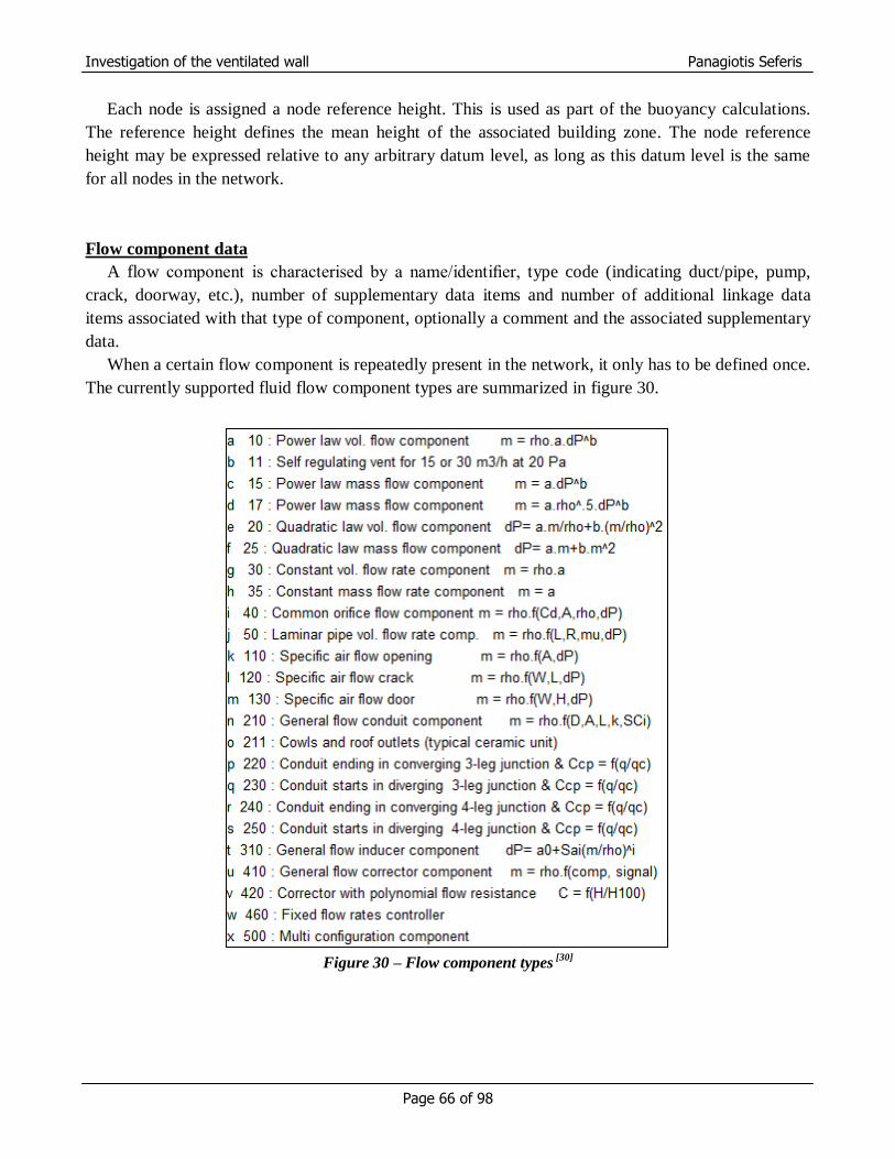
Investigation of the ventilated wall Panagiotis Seferis
Page 66 of 98
Each node is assigned a node reference height. This is used as part of the buoyancy calculations.
The reference height defines the mean height of the associated building zone. The node reference
height may be expressed relative to any arbitrary datum level, as long as this datum level is the same
for all nodes in the network.
Flow component data
A flow component is characterised by a name/identifier, type code (indicating duct/pipe, pump,
crack, doorway, etc.), number of supplementary data items and number of additional linkage data
items associated with that type of component, optionally a comment and the associated supplementary
data.
When a certain flow component is repeatedly present in the network, it only has to be defined once.
The currently supported fluid flow component types are summarized in figure 30.
Figure 30 – Flow component types
[30]
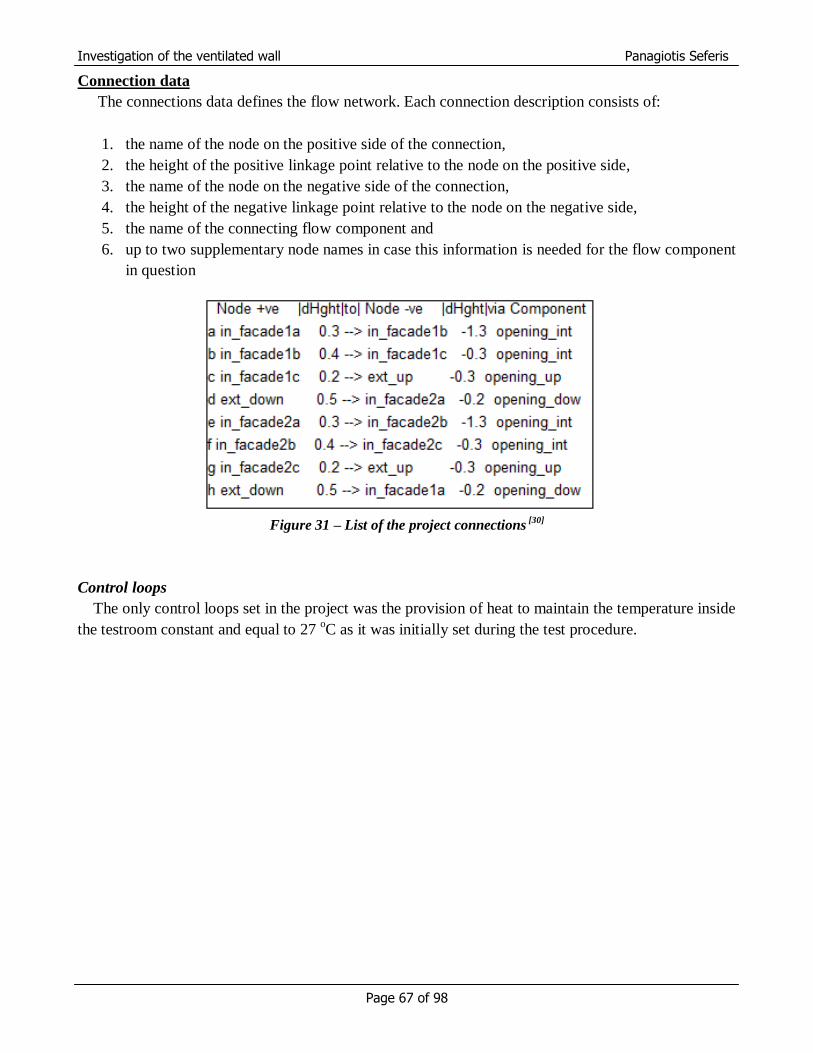
Investigation of the ventilated wall Panagiotis Seferis
Page 67 of 98
Connection data
The connections data defines the flow network. Each connection description consists of:
1. the name of the node on the positive side of the connection,
2. the height of the positive linkage point relative to the node on the positive side,
3. the name of the node on the negative side of the connection,
4. the height of the negative linkage point relative to the node on the negative side,
5. the name of the connecting flow component and
6. up to two supplementary node names in case this information is needed for the flow component
in question
Figure 31 – List of the project connections
[30]
Control loops
The only control loops set in the project was the provision of heat to maintain the temperature inside
the testroom constant and equal to 27 oC as it was initially set during the test procedure.
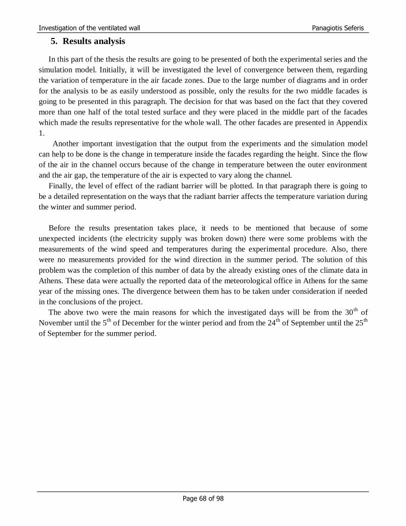
Investigation of the ventilated wall Panagiotis Seferis
Page 68 of 98
5. Results analysis
In this part of the thesis the results are going to be presented of both the experimental series and the
simulation model. Initially, it will be investigated the level of convergence between them, regarding
the variation of temperature in the air facade zones. Due to the large number of diagrams and in order
for the analysis to be as easily understood as possible, only the results for the two middle facades is
going to be presented in this paragraph. The decision for that was based on the fact that they covered
more than one half of the total tested surface and they were placed in the middle part of the facades
which made the results representative for the whole wall. The other facades are presented in Appendix
1.
Another important investigation that the output from the experiments and the simulation model
can help to be done is the change in temperature inside the facades regarding the height. Since the flow
of the air in the channel occurs because of the change in temperature between the outer environment
and the air gap, the temperature of the air is expected to vary along the channel.
Finally, the level of effect of the radiant barrier will be plotted. In that paragraph there is going to
be a detailed representation on the ways that the radiant barrier affects the temperature variation during
the winter and summer period.
Before the results presentation takes place, it needs to be mentioned that because of some
unexpected incidents (the electricity supply was broken down) there were some problems with the
measurements of the wind speed and temperatures during the experimental procedure. Also, there
were no measurements provided for the wind direction in the summer period. The solution of this
problem was the completion of this number of data by the already existing ones of the climate data in
Athens. These data were actually the reported data of the meteorological office in Athens for the same
year of the missing ones. The divergence between them has to be taken under consideration if needed
in the conclusions of the project.
The above two were the main reasons for which the investigated days will be from the 30th
of
November until the 5th
of December for the winter period and from the 24th
of September until the 25th
of September for the summer period.

Investigation of the ventilated wall Panagiotis Seferis
Page 69 of 98
5.1 Temperature variation in the air facade
Winter period
Figure 32 – Simulation and experimental temperature variation of the facade 1b during the winter period
(30th
of November to 5th
of December)
Figure 33 – Simulation and experimental temperature variation of the facade 2b during the winter period
(30th
of November to 5th
of December)
0
5
10
15
20
25
30
00:00 12:00 00:00 12:00 00:00 12:00 00:00 12:00 00:00 12:00 00:00 12:00 00:00
Tem
pe
ratu
re T
(o
C)
Time (Days)
facade 1b(sim)
Facade 1b(exp)
0
5
10
15
20
25
30
00:00 12:00 00:00 12:00 00:00 12:00 00:00 12:00 00:00 12:00 00:00 12:00 00:00
Tem
per
atu
re T
(o
C)
Time (Days)
Facade 2b(sim)
Facade 2b(exp)

Investigation of the ventilated wall Panagiotis Seferis
Page 70 of 98
Figure 34 – Simulation and experimental temperature difference of the facade 1b and 2b during the winter
period (30th
of November to 5th
of December)
In figures 32 and 33 is plotted the temperature variation inside the facades 1b and 2b during the
winter period according to the experimental and the simulation results. For each air zone the
temperature curve of the simulation and experimental output has the same shape but with differences
in their values.
Figure 34 shows this difference in temperature between the experimental and the simulation results
through time. A first notice is that the divergence is greater (with the experimental temperatures being
greater than the simulation ones) in the case of the wall with the radiant barrier (facade 2b) except the
period of every day when both the air zones reach their maximum temperature (around 12.00 at noon).
In that case the difference between them is greater, but with negative sign (the simulation temperatures
are greater than the corresponding experimental). In general, during the winter period, the highest
temperature difference was 4.5 oC in favour of the experimental temperature results and 6
oC in favour
of the simulation ones. Additionally the mean difference for the facade 1b is 1.55 oC while for the
facade 2b was slightly higher with a value of 2.19 oC.
-8
-6
-4
-2
0
2
4
6
00:00 12:00 00:00 12:00 00:00 12:00 00:00 12:00 00:00 12:00 00:00 12:00 00:00
Te
mp
era
ture
T (o
C)
Time (Days)
Facade 1b
Facade 2b
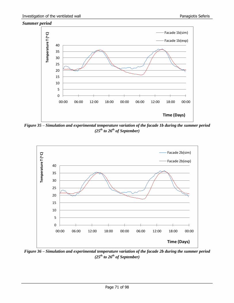
Investigation of the ventilated wall Panagiotis Seferis
Page 71 of 98
Summer period
Figure 35 – Simulation and experimental temperature variation of the facade 1b during the summer period
(25th
to 26th
of September)
Figure 36 – Simulation and experimental temperature variation of the facade 2b during the summer period
(25th
to 26th
of September)
0
5
10
15
20
25
30
35
40
00:00 06:00 12:00 18:00 00:00 06:00 12:00 18:00 00:00
Tem
pe
ratu
re T
(o
C)
Time (Days)
Facade 1b(sim)
Facade 1b(exp)
0
5
10
15
20
25
30
35
40
00:00 06:00 12:00 18:00 00:00 06:00 12:00 18:00 00:00
Tem
per
atu
re T
(o
C)
Time (Days)
Facade 2b(sim)
Facade 2b(exp)

Investigation of the ventilated wall Panagiotis Seferis
Page 72 of 98
Figure 37 – Simulation and experimental temperature difference of the facades 1b and 2b during the
summer period (25th
to 26th
of September)
The experimental and simulation results for the summer period as shown graphically in figures 35,
36 and especially 37 present a higher difference between them than the ones from the winter period.
The highest difference occurs on the second day at around 8.00 in the morning. At this time the
temperature given by the simulation model is around 10 oC higher than the corresponding
experimental in both the air facades. Consequently, the main differences in temperature results are
2.25 oC and 2.20
oC in facades 1b and 2b respectively.
An assumption for the temperature difference previously found is the fact that for the simulation
model, regarding the parameters that affect the flow in its air channel, it wasn‟t taken into account the
difference in pressure. The pressure coefficients for both the air openings were set to equal. Therefore,
the air flow inside the facades was caused only by temperature difference between the environment
and the air gap. The choice of that setting was the fact that there were a lot of measurements
(especially in the summer period) where the wind speed was equal to zero (figures 38 and 39). A
further investigation of the weather data in Athens (data taken by the meteorological institute for the
area of Athens) indicated that, in general, the wind speed values should have been greater. The result
was, according to the simulation model, a poorer circulation of air in the facades which allowed the
temperature rise.
-10
-8
-6
-4
-2
0
2
4Te
mp
era
ture
T (
o C
)
Time (Days)
Facade 1b
Facade 2b

Investigation of the ventilated wall Panagiotis Seferis
Page 73 of 98
Figure 38 – Wind speed vs time - winter period (30
th of November to 5
th of December)
Figure 39 – Wind speed vs time - summer period (25
th to 26
th of September)
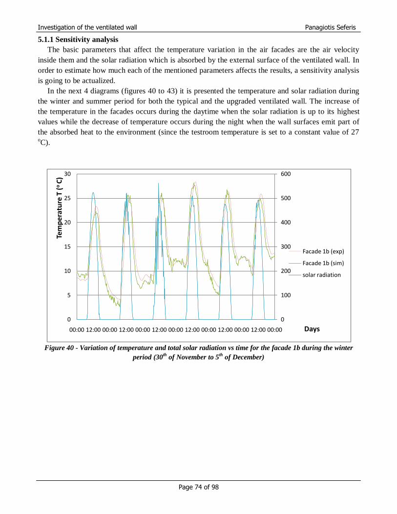
Investigation of the ventilated wall Panagiotis Seferis
Page 74 of 98
5.1.1 Sensitivity analysis
The basic parameters that affect the temperature variation in the air facades are the air velocity
inside them and the solar radiation which is absorbed by the external surface of the ventilated wall. In
order to estimate how much each of the mentioned parameters affects the results, a sensitivity analysis
is going to be actualized.
In the next 4 diagrams (figures 40 to 43) it is presented the temperature and solar radiation during
the winter and summer period for both the typical and the upgraded ventilated wall. The increase of
the temperature in the facades occurs during the daytime when the solar radiation is up to its highest
values while the decrease of temperature occurs during the night when the wall surfaces emit part of
the absorbed heat to the environment (since the testroom temperature is set to a constant value of 27 oC).
Figure 40 - Variation of temperature and total solar radiation vs time for the facade 1b during the winter
period (30th
of November to 5th
of December)
0
100
200
300
400
500
600
0
5
10
15
20
25
30
00:00 12:00 00:00 12:00 00:00 12:00 00:00 12:00 00:00 12:00 00:00 12:00 00:00
Tem
pe
ratu
re T
(o
C)
Days
Facade 1b (exp)
Facade 1b (sim)
solar radiation

Investigation of the ventilated wall Panagiotis Seferis
Page 75 of 98
Figure 41 - Variation of temperature and total solar radiation vs time for the facade 2b during the winter
period (30th
of November to 5th
of December)
Figure 42 - Variation of temperature and total solar radiation vs time for the facade 1b during the summer
period (25th
to 26th
of September)
0
100
200
300
400
500
600
0
5
10
15
20
25
30
00:00 12:00 00:00 12:00 00:00 12:00 00:00 12:00 00:00 12:00 00:00 12:00 00:00
Tem
per
atu
re T
(o
C)
Days
Facade 2b (exp)
Facade 2b (sim)
solar radiation
0
100
200
300
400
500
600
700
800
900
0
5
10
15
20
25
30
35
40
00:00 12:00 00:00 12:00 00:00
Tem
per
atu
re T
( o
C)
Time (h)
Facade 1b (exp)
Facade 1b (sim)
Solar radiation
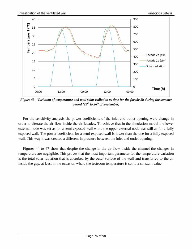
Investigation of the ventilated wall Panagiotis Seferis
Page 76 of 98
Figure 43 - Variation of temperature and total solar radiation vs time for the facade 2b during the summer
period (25th
to 26th
of September)
For the sensitivity analysis the power coefficients of the inlet and outlet opening were change in
order to alterate the air flow inside the air facades. To achieve that in the simulation model the lower
external node was set as for a semi exposed wall while the upper external node was still as for a fully
exposed wall. The power coefficient for a semi exposed wall is lower than the one for a fully exposed
wall. This way it was created a different in pressure between the inlet and outlet opening.
Figures 44 to 47 show that despite the change in the air flow inside the channel the changes in
temperature are negligible. This proves that the most important parameter for the temperature variation
is the total solar radiation that is absorbed by the outer surface of the wall and transferred to the air
inside the gap, at least in the occasion where the testroom temperature is set to a constant value.
0
100
200
300
400
500
600
700
800
900
0
5
10
15
20
25
30
35
40
00:00 12:00 00:00 12:00 00:00
Tem
per
atu
re T
(oC
)
Time (h)
Facade 2b (exp)
Facade 2b (sim)
Solar radiation

Investigation of the ventilated wall Panagiotis Seferis
Page 77 of 98
Winter period
Figure 44 – Temperature variation inside the air facade 1b of the simulation model with and without
pressure difference between the openings during the winter period ((30th
of November to 5th
of December)
Figure 45 – Temperature variation inside the air facade 2b of the simulation model with and without
pressure difference between the openings during the winter period ((30th
of November to 5th
of December)
0
5
10
15
20
25
30
00:00 12:00 00:00 12:00 00:00 12:00 00:00 12:00 00:00 12:00 00:00 12:00 00:00
Tem
per
atu
re T
(o
C)
Time (Days)
facade 1b(sim)
Facade 1b(sim pres. diff)
0
5
10
15
20
25
30
00:00 12:00 00:00 12:00 00:00 12:00 00:00 12:00 00:00 12:00 00:00 12:00 00:00
Tem
per
atu
re T
(o
C)
Time (Days)
Facade 2b(sim)
Facade 2b(sim pres. diff)
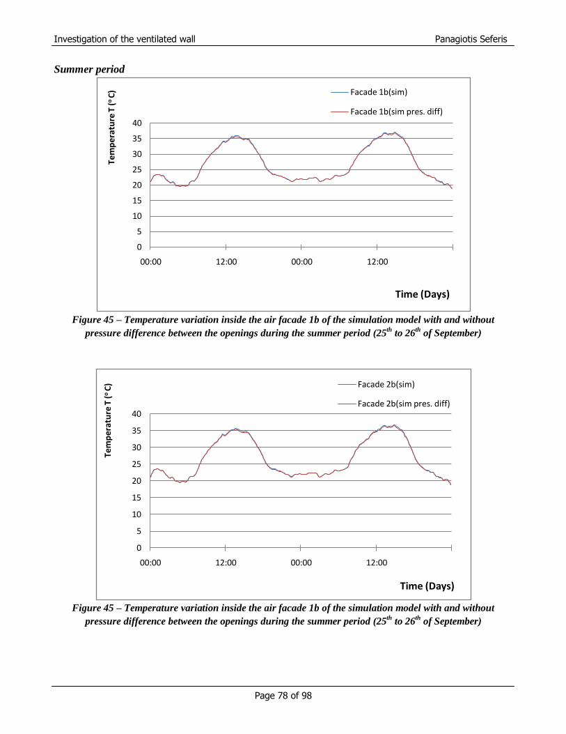
Investigation of the ventilated wall Panagiotis Seferis
Page 78 of 98
Summer period
Figure 45 – Temperature variation inside the air facade 1b of the simulation model with and without
pressure difference between the openings during the summer period (25th
to 26th
of September)
Figure 45 – Temperature variation inside the air facade 1b of the simulation model with and without
pressure difference between the openings during the summer period (25th
to 26th
of September)
0
5
10
15
20
25
30
35
40
00:00 12:00 00:00 12:00
Tem
per
atu
re T
(o
C)
Time (Days)
Facade 1b(sim)
Facade 1b(sim pres. diff)
0
5
10
15
20
25
30
35
40
00:00 12:00 00:00 12:00
Tem
per
atu
re T
(o
C)
Time (Days)
Facade 2b(sim)
Facade 2b(sim pres. diff)
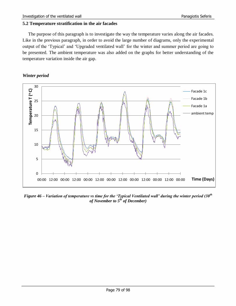
Investigation of the ventilated wall Panagiotis Seferis
Page 79 of 98
5.2 Temperature stratification in the air facades
The purpose of this paragraph is to investigate the way the temperature varies along the air facades.
Like in the previous paragraph, in order to avoid the large number of diagrams, only the experimental
output of the „Typical‟ and „Upgraded ventilated wall‟ for the winter and summer period are going to
be presented. The ambient temperature was also added on the graphs for better understanding of the
temperature variation inside the air gap.
Winter period
Figure 46 – Variation of temperature vs time for the ‘Typical Ventilated wall’ during the winter period (30
th
of November to 5th
of December)
0
5
10
15
20
25
30
00:00 12:00 00:00 12:00 00:00 12:00 00:00 12:00 00:00 12:00 00:00 12:00 00:00
Tem
per
atu
re T
(o
C)
Time (Days)
Facade 1c
Facade 1b
Facade 1a
ambient temp
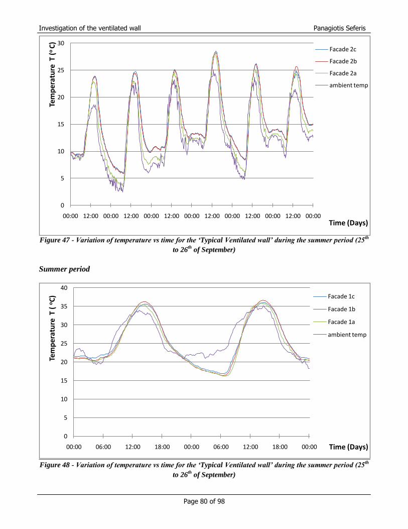
Investigation of the ventilated wall Panagiotis Seferis
Page 80 of 98
Figure 47 - Variation of temperature vs time for the ‘Typical Ventilated wall’ during the summer period (25
th
to 26th
of September)
Summer period
Figure 48 - Variation of temperature vs time for the ‘Typical Ventilated wall’ during the summer period (25
th
to 26th
of September)
0
5
10
15
20
25
30
00:00 12:00 00:00 12:00 00:00 12:00 00:00 12:00 00:00 12:00 00:00 12:00 00:00
Tem
pe
ratu
re T
(o
C)
Time (Days)
Facade 2c
Facade 2b
Facade 2a
ambient temp
0
5
10
15
20
25
30
35
40
00:00 06:00 12:00 18:00 00:00 06:00 12:00 18:00 00:00
Tem
pe
ratu
re T
( o
C)
Time (Days)
Facade 1c
Facade 1b
Facade 1a
ambient temp

Investigation of the ventilated wall Panagiotis Seferis
Page 81 of 98
Figure 49 - Variation of temperature vs time for the ‘Upgraded Ventilated wall’ during the summer period
(25th
to 26th
of September)
There are two main questions that are tried to be answered in this paragraph; the temperature
variation in the air facades of each wall comparing to each other and to the ambient temperature.
During the winter period (Figures 46 and 47) the temperature variation of the air facades for both
the walls are of similar shape to each other and also similar but always higher to the ambient
temperature. This indicates that the air gap works as an additional insulation which actually helps to
the decreasing of the overall heat losses. The lowest facades (1a and 2a) are the ones with the lowest
temperature comparing to the other since the air entering the channel keeps absorbing heat as it rises
along the gap. The absorption of heat can be explained by the fact that the ambient temperature is
always lower than 27 oC which is the constant temperature of the testroom and the wall that separates
the testroom and the air gap is obviously not well enough insulated.
In the summer period as the ambient temperature become greater than 27 oC at times the lowest
facades are not always the ones with the lowest temperature (Figure 49) since the circulating air tends
to lower its temperature. Another important point that needs to be noticed is that the temperature in the
air channel during the night time is lower than the ambient. This notice leads to the conclusion that the
air gap, during the night hours, actually works as a chilling zone.
The differences in temperature of the air zones to each other and between them and the ambient one
is an indicator of the air flowrate inside the channel. The lower the difference in temperature between
two consecutive air zones or between them and the ambient temperature the highest the air mass
0
5
10
15
20
25
30
35
40
00:00 06:00 12:00 18:00 00:00 06:00 12:00 18:00 00:00
Tem
per
atu
re T
(oC
)
Time (Days)
Facade 2c
Facade 2b
Facade 2a
ambient temp

Investigation of the ventilated wall Panagiotis Seferis
Page 82 of 98
flowrate inside the channel. If the air flowrate is low the result is that the air has more time to
exchange heat with the surfaces of the inner walls of the channel. This exchange leads to the alteration
of the air temperature along the gap.
5.3 Level of effect of the radiant barrier
From the beginning of the ventilated wall construction a very important issue was how much and in
which way the radiant barrier that was installed on one half of the wall would affect the temperature of
the circulating air along the air gap. In the next figures the temperature variation in the middle air
facade zones is presented (Facades 1b and 2b). The rest of the air zones are represented in the
Appendix 2. In each figure of the experimental and simulation output there are two curves representing
the temperature variation of each air facade zone in the „Typical ventilated wall‟ compared with the
corresponding air facade zone in the „Upgraded ventilated wall‟ for both the winter and summer
period. This way the resulting comparison would indicate only level of impact because of the radiant
barrier installation on the ventilated wall. A third graph is also provided to plot the difference between
the experimental and simulation results.
Winter period
Experimental data
Figure 50 – Variation of temperature vs time in the air facades 1b & 2b during the winter period (30
th of
November to 5th
of December)
0
5
10
15
20
25
30
00:00 12:00 00:00 12:00 00:00 12:00 00:00 12:00 00:00 12:00 00:00 12:00 00:00
Tem
per
atu
re T
(o
C)
Time (days)
Facade 1b
Facade 2b
ambient temp

Investigation of the ventilated wall Panagiotis Seferis
Page 83 of 98
Simulation data
Figure 51 – Variation of temperature vs time in the air facades 1b & 2b during the winter period (30
th of
November to 5th
of December)
Figure 52 - Simulation and experimental temperature difference of the facades 1b and 2b during the winter
period (30th
of November to 5th
of December)
0
5
10
15
20
25
30
00:00 12:00 00:00 12:00 00:00 12:00 00:00 12:00 00:00 12:00 00:00 12:00 00:00
Tem
per
atu
re T
(o
C)
Days
Facade 1b
Facade 2b
ambient temp
-2.25
-2
-1.75
-1.5
-1.25
-1
-0.75
-0.5
-0.25
0
0.25
0.5
0.75
00:00 12:00 00:00 12:00 00:00 12:00 00:00 12:00 00:00 12:00 00:00 12:00 00:00Tem
per
atu
re T
(o
C)
Days
Facade b (sim)
Facade b (exp)

Investigation of the ventilated wall Panagiotis Seferis
Page 84 of 98
Figures 50 and 51 show an obvious difference between the experimental and the simulation results
regarding the temperature variation if the air zones 1b and 2b. This difference is clearer plotted in
figure 52. According to the experimental results, the radiant barrier that was added in half of the
ventilated wall is responsible for keeping the temperature higher inside air facade 2b during night time
and slightly lower during day time. This happens because the radiant barrier actually works as an
additional insulation making the response of the air zones slower. The effect is more severe in the
night hours where the temperature difference between the air facade 2b and air facade 1b reaches the
value of around 1.8 oC.
Summer period
Experimental data
Figure 53 - Temperature vs time in the air facades 1b & 2b during the summer period
(25th
to 26th
of September)
0
5
10
15
20
25
30
35
40
00:00 12:00 00:00 12:00 00:00
Tem
per
atu
re T
( o
C)
Time (days)
Facade 1b
Facade 2b
ambient temp

Investigation of the ventilated wall Panagiotis Seferis
Page 85 of 98
Simulation Data
Figure 54 - Temperature vs time in the air facades 1b & 2b during the summer period
(25th
to 26th
of September)
Figure 55 - Simulation and experimental temperature difference of the facades 1b and 1b during the summer
period (25th
to 26th
of September)
0
5
10
15
20
25
30
35
40
00:00 12:00 00:00 12:00 00:00
Tem
per
atu
re T
( o
C)
Time (days)
Facade 1b
Facade 2b
ambient temp
-1.5
-1.25
-1
-0.75
-0.5
-0.25
0
0.25
0.5
0.75
1
1.25
00:00 06:00 12:00 18:00 00:00 06:00 12:00 18:00
Tem
per
atu
re T
( o
C)
Time (days)
Facade b (sim)
Facade b (exp)
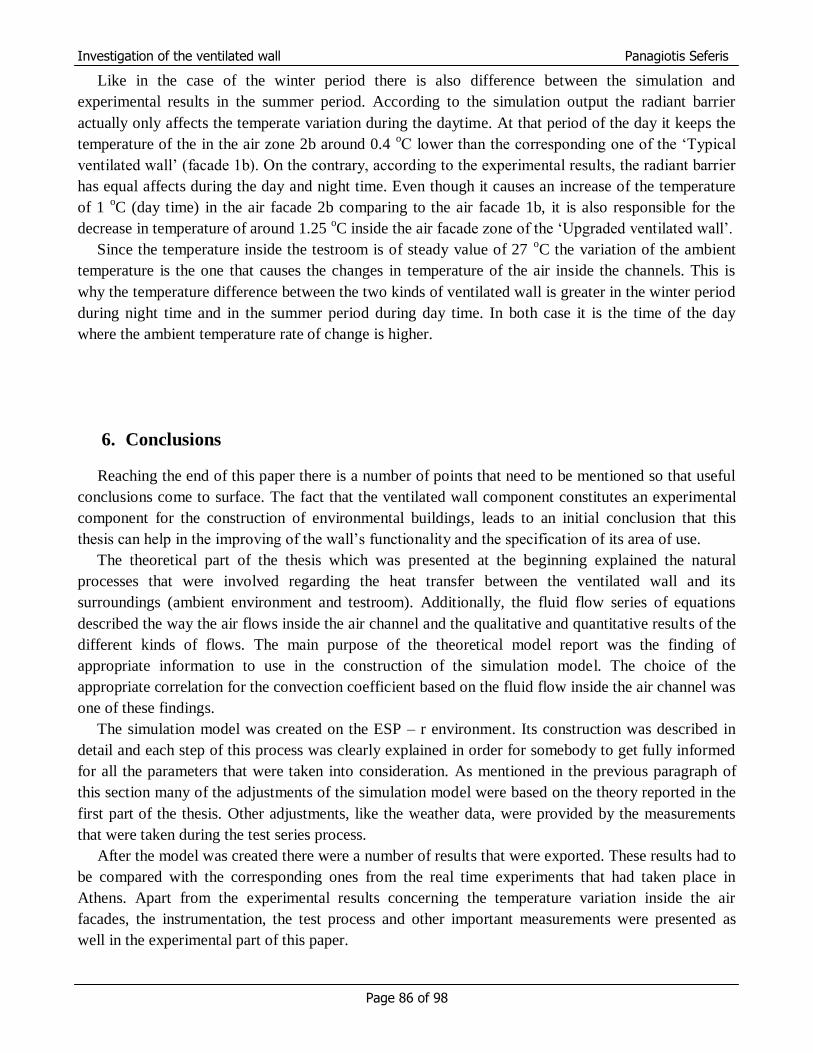
Investigation of the ventilated wall Panagiotis Seferis
Page 86 of 98
Like in the case of the winter period there is also difference between the simulation and
experimental results in the summer period. According to the simulation output the radiant barrier
actually only affects the temperate variation during the daytime. At that period of the day it keeps the
temperature of the in the air zone 2b around 0.4 oC lower than the corresponding one of the „Typical
ventilated wall‟ (facade 1b). On the contrary, according to the experimental results, the radiant barrier
has equal affects during the day and night time. Even though it causes an increase of the temperature
of 1 oC (day time) in the air facade 2b comparing to the air facade 1b, it is also responsible for the
decrease in temperature of around 1.25 oC inside the air facade zone of the „Upgraded ventilated wall‟.
Since the temperature inside the testroom is of steady value of 27 oC the variation of the ambient
temperature is the one that causes the changes in temperature of the air inside the channels. This is
why the temperature difference between the two kinds of ventilated wall is greater in the winter period
during night time and in the summer period during day time. In both case it is the time of the day
where the ambient temperature rate of change is higher.
6. Conclusions
Reaching the end of this paper there is a number of points that need to be mentioned so that useful
conclusions come to surface. The fact that the ventilated wall component constitutes an experimental
component for the construction of environmental buildings, leads to an initial conclusion that this
thesis can help in the improving of the wall‟s functionality and the specification of its area of use.
The theoretical part of the thesis which was presented at the beginning explained the natural
processes that were involved regarding the heat transfer between the ventilated wall and its
surroundings (ambient environment and testroom). Additionally, the fluid flow series of equations
described the way the air flows inside the air channel and the qualitative and quantitative results of the
different kinds of flows. The main purpose of the theoretical model report was the finding of
appropriate information to use in the construction of the simulation model. The choice of the
appropriate correlation for the convection coefficient based on the fluid flow inside the air channel was
one of these findings.
The simulation model was created on the ESP – r environment. Its construction was described in
detail and each step of this process was clearly explained in order for somebody to get fully informed
for all the parameters that were taken into consideration. As mentioned in the previous paragraph of
this section many of the adjustments of the simulation model were based on the theory reported in the
first part of the thesis. Other adjustments, like the weather data, were provided by the measurements
that were taken during the test series process.
After the model was created there were a number of results that were exported. These results had to
be compared with the corresponding ones from the real time experiments that had taken place in
Athens. Apart from the experimental results concerning the temperature variation inside the air
facades, the instrumentation, the test process and other important measurements were presented as
well in the experimental part of this paper.

Investigation of the ventilated wall Panagiotis Seferis
Page 87 of 98
The comparison of the experimental and the simulation model results regarding the temperature
variation in the air facades showed satisfactory levels of convergence. The only occasion in which
there was a significant divergence between the results was for the summer period during the night
hours. A sensitivity analysis was carried out by changing the flow rate in the facades and checking if
this change would affect the resulting temperature alteration inside the air channel. Up until then, the
air circulation, for the simulation model, was set to be dependent only by the difference in temperature
between the environment and the air gap since the pressure coefficients of the inlet and outlet openings
were set to equal. Unfortunately, there were no experimental measurements about these pressure
coefficients and this was why, they were used preset values from ESP – r.
The effectiveness of the radiant barrier was tested through the difference in temperature that
occurred between the corresponding air zones of the „Typical‟ and „Upgraded ventilated wall‟. Its
usage can be characterized as positive since it managed to keep the air facade zones of the „Upgraded
ventilated wall‟ warmer during the winter period (especially during night time when the need for heat
is higher). On the other hand, during the summer period, it succeeded on keeping the air facade zones
in levels less warm than in the corresponding ones of the „Typical ventilating wall‟.
In order to come to more sufficient results about the functionality of a wall component like the
„Ventilated wall component‟ it would be expedient to run a similar process like the one of this thesis
but in a real time building and possibly without setting the internal temperature at a constant value.
Also the use of some additional instrumentation for the measurements of the flowrate in the facades
and for the pressure coefficients in the inlet and outlet openings could significantly help on that
investigation. The main differences between the experimental and the simulation results could be
solved if the above parameters can be set.
In general the „Ventilated wall component‟ constitutes a very interesting project which can be
commercialized in the rear future. This thesis as mentioned just earlier in this paragraph proved the
positive functions that provides regarding the levels of air temperature that keeps inside its facades. A
further number of experiments should focus on the testing of new construction materials for the wall.
But the most important is for the total cost of it construction to be kept in low levels. A future
econometric analysis would be very important in order to provide important information of how much
the use of more sophisticated materials which will increase its total performance would affect its final
prise of construction.
This investigation of the „Ventilated wall components‟ with and without the addition of the radiant
barrier could be actualized in a different city than Athens, with different weather characteristics. A
colder city like Glasgow could be an appropriate choice. This can lead to a more detailed amount of
information about the advantages and disadvantages of this wall component.

Investigation of the ventilated wall Panagiotis Seferis
Page 88 of 98
References
1. Chiras, D., “The Solar House: Passive Heating and Cooling”, Chelsea Green Publishing
Company, 2002.
2. Michael F. Hordeski, „Dictionary of Energy Efficiency Technologies‟, The Fairmont Press,
Inc., 2004
3. Duffie J.A. and Beckman W.A. Solar Engineering of Thermal Processes, 2nd ed. pp. Wiley
Interscience, New York, 1991.
4. Ní Riain, C. M. Kolokotroni, M. Davies, J. Fisher, M. White, J. Littler, "Cooling Effectiveness
of South Facade Passive Stacks in a Naturally Ventilated Office Building - Case Study". Indoor
and Built Environment, 1999.
5. Dai, Y. J.; K. Sumathy, R. Z. Wang, and Y. G. Li, "Enhancement of natural ventilation in a
solar house with a solar chimney and a solid adsorption cooling cavity", Elsevier Science B.V,
2003.
6. Incropera, F. and D. DeWitt, “Fundamentals of Heat and Mass Transfer”, fourth edition, John
Wiley & Sons, 1996.
7. David P. Kessler, Robert A. Greenkorn, “Momentum, Heat, and Mass Transfer Fundamentals”,
CRC Press, 1999
8. McAdams, W. H., “Heat Transmission”, New York, McGraw-Hill, 1954
9. Ito, N., K. Kimura and J. Oka, “A field experiment study on the convective heat transfer
coefficient on exterior surface of a building”, ASHRAE Transactions, 1972.
10. Kimura, K., “Scientific basis of air conditioning”, London, Applied Science Publishers, Ltd.,
1977
11. Yazdanian, M. and J. H. Klems, “Measurement of the exterior convective film coefficient for
windows in low-rise buildings”. Proceedings of the ASHRAE Winter Meeting, Jan 23-26
1994, New Orleans, USA, 1994.
12. Sandberg, M. and B. Moshfegh, “Buoyancy-induced air flow in photovoltaic facades effect of
geometry of the air gap and location of solar cell modules”. Building and Environment Vol. 37,
2002.
13. J. S. Turner, “Buoyancy Effects in Fluids”, Cambridge University Press, 1980
14. Joseph A. Schetz, Allen E. Fuhs, “Fundamentals of Fluid Mechanics”, Wiley-IEEE, 1999

Investigation of the ventilated wall Panagiotis Seferis
Page 89 of 98
15. Shah R.K. and A.L. London, 1978, 'Laminar Flow Forced Convection in Ducts', Supplement 1
in Advances in Heat Transfer, Academic, NY, 1978.
16. Munson, B., D. Young and T. Okiishi, “Fundamentals of Fluid Mechanics”, third edition. New
York, U.S.A., John Wiley & Sons, 1998.
17. Vedat S. Arpaci, Yıldız Bayazıtoğlu, „Fundamentals of natural convection‟, American Society
of Mechanical Engineers, 1990.
18. Ostrach, S., “An Analysis of Laminar-Free-Convection Flow and Heat Transfer about a Flat
Plate Paralell to the Direction of the Generation Body Force”, NACA Technical Report 1111,
1953.
19. Holman, J. P., “Heat Transfer”, Ninth Edition, McGraw-Hill, 2002.
20. Churchill, S. W. and H. H. S. Chu, “Correlating equations for laminar and turbulent free
convection from a vertical plate”, International Journal of Heat and Mass Transfer, 1975.
21. Bejan, A., “Convective heat transfer”, New York, John Wiley & Sons, 1984
22. G. A. Tokaty, „A History and Philosophy of Fluid Mechanics‟, Courier Dover Publications,
1994.
23. Churchill, S. W. and Usagi, “A general expression of rates of heat transfer and other
phenomena”, A.I. CHE. J. Vol. 18, 1972.
24. Bar-Cohen, A. and W. M. Rohsenow, “Thermally Optimum Spacing of Vertical, Natural
Convection Cooled Parallel Plates”. Journal of Heat Transfer, Transactions ASME Vol. 106,
1984.
25. Sparrow, E. M. and L. F. A. Azevedo, “Vertical-channel Natural Convection Spanning
Between the Fully-Developed Limit and the Single-Plate Boundary-Layer Limit”, International
Journal of Heat and Mass Transfer Vol. 28, 1985.
26. Energy Systems Research Unit, „The ESP – r System for Building Energy Simulation User
Guide Version 10‟, University of Strathclyde, October 2002.
27. Dimoudi A., Lykoudis S., Androutsopoulos A., „Testing of the Prokelyfos ventilated wall
component at CRES test site‟, Final Technical Report AIRinSTRUCT project: „Integration of
Advanced Ventilated Building Components and Structures for Reduction of Energy
Consumption in Buildings, EC-DG XII, Contract No JOE3 – CT97 – 7003, Passive Solar and
Hybrid Systems Department - Centre for Renewable Energy Sources (CRES), 2000.
28. Dimoudi A., Androutsopoulos A., Lykoudis S. „Energy conservation in buildings with
integration of advanced ventilated wall components‟, 22nd
annual AIVC conference „Market

Investigation of the ventilated wall Panagiotis Seferis
Page 90 of 98
Opportunities for Advanced Ventilation Technology‟,, Bath, United Kingdom, 11 – 14
September 2001.
Pictures references
I. http://livemodern.com/buildblogs
II. http://livemodern.com/designblogs
III. www.azsolarcenter.com
IV. www.brightworks.net
V. http://habitbydesign.blogspot.com
VI. Dimoudi A., Lykoudis S., Androutsopoulos A., „Testing of the Prokelyfos ventilated wall
component at CRES test site‟, Final Technical Report AIRinSTRUCT project: „Integration of
Advanced Ventilated Building Components and Structures for Reduction of Energy
Consumption in Buildings, EC-DG XII, Contract No JOE3 – CT97 – 7003, Passive Solar and
Hybrid Systems Department - Centre for Renewable Energy Sources (CRES), 2000.

Investigation of the ventilated wall Panagiotis Seferis
Page 91 of 98
Appendix 1
Winter period
Figure 56 – Simulation and experimental temperature variation of the facade 1a during the winter period
(30th
of November to 5th
of December)
Figure 57 – Simulation and experimental temperature variation of the facade 2a during the winter period
(30th
of November to 5th
of December)
0
5
10
15
20
25
30
00:00 12:00 00:00 12:00 00:00 12:00 00:00 12:00 00:00 12:00 00:00 12:00 00:00
Tem
pe
ratu
re T
(o
C)
Time (Days)
Facade 1a(sim)
Facade 1a(exp)
0
5
10
15
20
25
30
00:00 12:00 00:00 12:00 00:00 12:00 00:00 12:00 00:00 12:00 00:00 12:00 00:00
Tem
per
atu
re T
(o
C)
Time (Days)
Facade 2a(sim)
Facade 2a(exp)

Investigation of the ventilated wall Panagiotis Seferis
Page 92 of 98
Figure 58 – Simulation and experimental temperature difference of the facade 1a and 2a during the winter
period (30th
of November to 5th
of December)
Figure 59 – Simulation and experimental temperature variation of the facade 1c during the winter period
(30th
of November to 5th
of December)
-8
-6
-4
-2
0
2
4
6
00:00 12:00 00:00 12:00 00:00 12:00 00:00 12:00 00:00 12:00 00:00 12:00 00:00
Tem
per
atu
re T
(o C
)
Time (Days)
without rad_barrier
with rad_barrier
0
5
10
15
20
25
30
00:00 12:00 00:00 12:00 00:00 12:00 00:00 12:00 00:00 12:00 00:00 12:00 00:00
Tem
per
atu
re T
(o
C)
Time (Days)
Facade 1c(sim)
Facade 1c(exp)

Investigation of the ventilated wall Panagiotis Seferis
Page 93 of 98
Figure 60 – Simulation and experimental temperature variation of the facade 2c during the winter period
(30th
of November to 5th
of December)
Figure 61 – Simulation and experimental temperature difference of the facade 1b and 2b during the winter
period (30th
of November to 5th
of December)
0
5
10
15
20
25
30
00:00 12:00 00:00 12:00 00:00 12:00 00:00 12:00 00:00 12:00 00:00 12:00 00:00
Tem
pe
ratu
re T
(o
C)
Time (Days)
Facade 2c(sim)
Facade 2c(exp)
-5
-4
-3
-2
-1
0
1
2
3
4
5
00:00 12:00 00:00 12:00 00:00 12:00 00:00 12:00 00:00 12:00 00:00 12:00 00:00
Tem
per
atu
re T
(o
C)
Time (Days)
without rad_barrier
with rad_barrier

Investigation of the ventilated wall Panagiotis Seferis
Page 94 of 98
Summer period
Figure 62 – Simulation and experimental temperature variation of the facade 1a during the summer period
(25th
to 26th
of September)
Figure 63 – Simulation and experimental temperature variation of the facade 2a during the summer period
(25th
to 26th
of September)
0
5
10
15
20
25
30
35
40
00:00 06:00 12:00 18:00 00:00 06:00 12:00 18:00 00:00
Tem
pe
ratu
re T
(o
C)
Time (Days)
Facade 1a(sim)
Facade 1a(exp)
0
5
10
15
20
25
30
35
40
00:00 06:00 12:00 18:00 00:00 06:00 12:00 18:00 00:00
Tem
per
atu
re T
(o
C)
Time (Days)
Facade 2a(sim)
Facade 2a(exp)
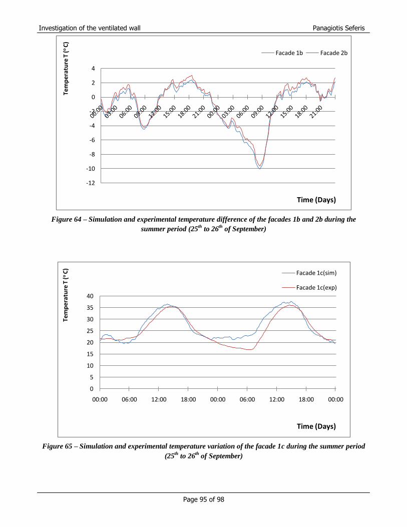
Investigation of the ventilated wall Panagiotis Seferis
Page 95 of 98
Figure 64 – Simulation and experimental temperature difference of the facades 1b and 2b during the
summer period (25th
to 26th
of September)
Figure 65 – Simulation and experimental temperature variation of the facade 1c during the summer period
(25th
to 26th
of September)
-12
-10
-8
-6
-4
-2
0
2
4Te
mp
erat
ure
T (
o C
)
Time (Days)
Facade 1b Facade 2b
0
5
10
15
20
25
30
35
40
00:00 06:00 12:00 18:00 00:00 06:00 12:00 18:00 00:00
Tem
per
atu
re T
(o
C)
Time (Days)
Facade 1c(sim)
Facade 1c(exp)
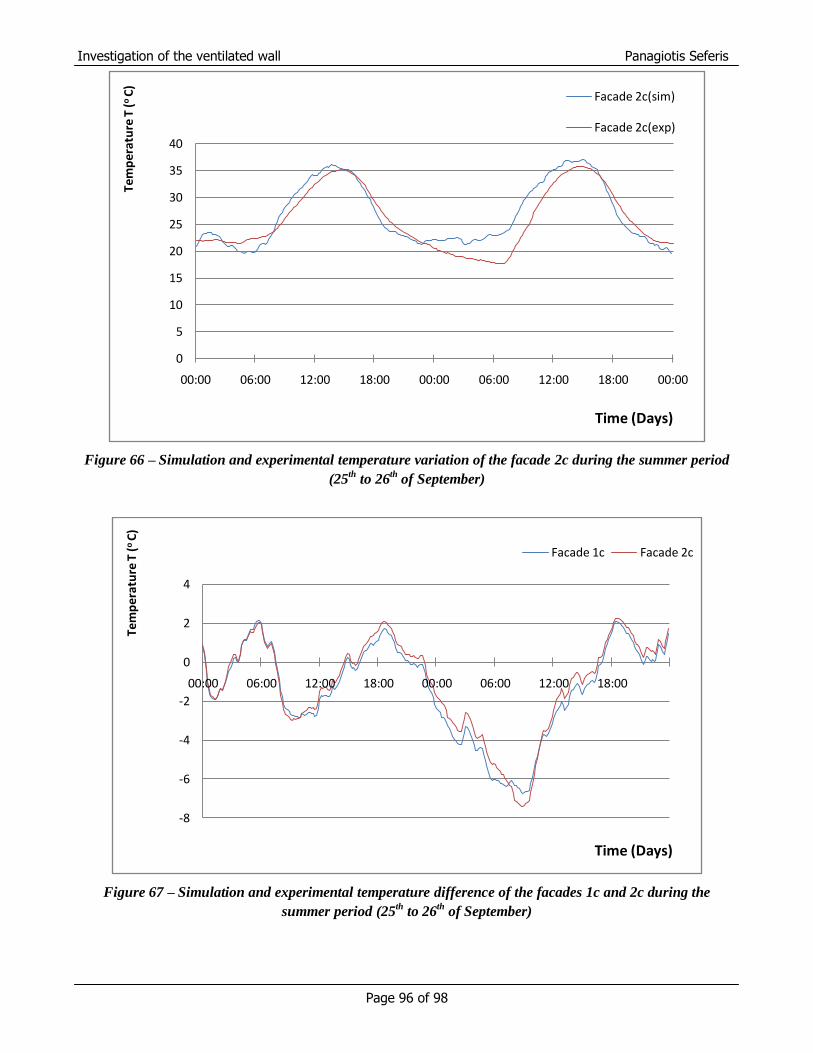
Investigation of the ventilated wall Panagiotis Seferis
Page 96 of 98
Figure 66 – Simulation and experimental temperature variation of the facade 2c during the summer period
(25th
to 26th
of September)
Figure 67 – Simulation and experimental temperature difference of the facades 1c and 2c during the
summer period (25th
to 26th
of September)
0
5
10
15
20
25
30
35
40
00:00 06:00 12:00 18:00 00:00 06:00 12:00 18:00 00:00
Tem
per
atu
re T
(o
C)
Time (Days)
Facade 2c(sim)
Facade 2c(exp)
-8
-6
-4
-2
0
2
4
00:00 06:00 12:00 18:00 00:00 06:00 12:00 18:00
Tem
per
atu
re T
(o
C)
Time (Days)
Facade 1c Facade 2c

Investigation of the ventilated wall Panagiotis Seferis
Page 97 of 98
Appendix 2
Winter period
Figure 68 – Variation of temperature vs time in the air facades 1a & 2a during the winter period (30th
of
November to 5th
of December)
Figure 69 – Variation of temperature vs time in the air facades 1c & 2c during the winter period (30th
of
November to 5th
of December)
0
5
10
15
20
25
30
00:00 12:00 00:00 12:00 00:00 12:00 00:00 12:00 00:00 12:00 00:00 12:00 00:00
Tem
per
atu
re T
(o
C)
Days
Facade 1a
Facade 2a
ambient temp
0
5
10
15
20
25
30
00:00 12:00 00:00 12:00 00:00 12:00 00:00 12:00 00:00 12:00 00:00 12:00 00:00
Tem
pe
ratu
re T
(o
C)
Days
Facade 1c
Facade 2c
ambient temp

Investigation of the ventilated wall Panagiotis Seferis
Page 98 of 98
Summer period
Figure 70 - Temperature vs time in the air facades 1a & 2a during the summer period
(25th
to 26th
of September)
Figure 71 - Temperature vs time in the air facades 1c & 2c during the summer period
(25th
to 26th
of September)
0
5
10
15
20
25
30
35
40
00:00 06:00 12:00 18:00 00:00 06:00 12:00 18:00 00:00
Tem
per
atu
re T
( o
C)
Time (days)
Facade 1a
Facade 2a
ambient temp
0
5
10
15
20
25
30
35
40
00:00 06:00 12:00 18:00 00:00 06:00 12:00 18:00 00:00
Tem
pe
ratu
re T
( o
C)
Time (days)
Facade 1c
Facade 2c
ambient temp