munich personal repec archive - uni-muenchen.de · munich personal repec archive ... a...
TRANSCRIPT

MPRAMunich Personal RePEc Archive
Financial Deregulation and ProfitEfficiency: A Non-parametric Analysis ofIndian Banks
Saibal Ghosh
Reserve Bank of India
November 2009
Online at https://mpra.ub.uni-muenchen.de/24292/MPRA Paper No. 24292, posted 10. August 2010 05:54 UTC

Financial Deregulation and Profit Efficiency: A Non-parametric Analysis of Indian Banks*
Abhiman Das@ Massachusetts Institute of Technology
and Reserve Bank of India
Saibal Ghosh& Reserve Bank of India [email protected]
Abstract The paper investigates the performance of Indian commercial banking sector during the post reform period 1992-2004. The results indicate high levels of efficiency in costs and lower levels in profits, reflecting the importance of inefficiencies on the revenue side of banking activity. The decomposition of profit efficiency shows that a large portion of outlay lost is due to allocative inefficiency. The proximate determinants of profit efficiency appears to suggest that big state-owned banks performed reasonably well and are more likely to operate at higher levels of profit efficiency. A close relationship is observed between efficiency and soundness as determined by bank’s capital adequacy ratio. The empirical results also show that the profit efficient banks are those that have, on an average, less non-performing loans. JEL classification: D61; G21; G34 Keywords: Indian Banks; Deregulation; Profit efficiency; DEA model
* This work was initiated when the first author was a post-doctoral fellow at MIT. The authors would like to thank, without implicating, two anonymous referees for their insightful and painstaking comments on an earlier draft which greatly improved the clarity and exposition of the paper. The opinion expressed in the paper are the sole responsibility of the authors and do not necessarily reflect the position of the institutions with which they are affiliated. @Corresponding author. Department of Statistical Analysis and Computer Services, Reserve Bank of India, Bandra-Kurla Complex, Bandra(E), Mumbai - 400051 INDIA. &Department of Economic Analysis and Policy, Reserve Bank of India, Fort, Mumbai 400001 INDIA.

1
Financial Deregulation and Profit Efficiency: A Non-parametric Analysis of Indian Banks *
I. Introduction
In recent years, a growing body of literature has analysed the efficiency of banks and financial
institutions, mostly centering around costs and technical efficiency and predominantly on
developed countries. On the cost side, differences in average costs have been examined by
estimating economies of scale and, to a lesser extent, of scope economies. As against this,
there is limited empirical evidence on profit efficiency of banks. However, the objective of
profit maximization not only requires that goods and services be produced at a minimum cost,
it also demands the maximization of revenues. Banks that show the highest inefficiencies and
incur the highest cost might be able to generate greater profits than more cost efficient banks
(Berger and Humphrey, 1997; Berger and Mester, 2003). Computing profit efficiency,
therefore, constitutes a more important source of information for bank management.
The paper addresses this issue in a developing country context, focusing on India as a case
study. A number of factors make the study of banking in India an interesting one. First, over
the 1990s, India has undergone significant deregulation with the objectives of enhancing
efficiency, productivity and profitability of banks. Salient among the measures introduced
include (a) lowering of statutory reserve requirements; (b) liberalizing the interest rate regime,
allowing banks the freedom to determine their deposit and lending rates; (c) infusing
competition by allowing more liberal entry of foreign banks and permitting the establishment
of de novo private banks; (d) introduction of micro-prudential measures such as capital
adequacy requirements, income recognition, asset classification and provisioning norms for
loan classification as also exposure norms and accounting standards; (e) diversifying the
ownership base of state-owned banks by enabling them to raise up to 49% of their capital from
the market and (f) mandating greater disclosures in the balance sheets to ensure greater
transparency and market discipline. Second, India is one of the largest and fastest growing
emerging economies with a gamut of banks across different ownership categories.1 It would be
* This work was initiated when the first author was a post-doctoral fellow at MIT. The authors would like to thank, without implicating, two anonymous referees for their insightful and painstaking comments on an earlier draft which greatly improved the clarity and exposition of the paper. The opinion expressed in the paper are the sole responsibility of the authors and do not necessarily reflect the position of the institutions with which they are affiliated. 1The banking system in India comprises commercial and co-operative banks, of which the former accounts for around 95% of banking system assets. The commercial banking sector consists of state-owned or public sector banks, Indian private banks and foreign banks operating in India. State-owned banks cover nationalised banks (majority equity holding being with the Government), the State Bank of India (majority equity holding being with the Reserve Bank of India) and its associate banks (majority

2
of interest to examine if the diversification of the ownership of state-owned banks and the
penetration of private and foreign banks has had an impact on profit efficiency. Third, studies
on efficiency in Indian banks have typically examined the cost and technical efficiency
(Bhattacharya et al., 1997; Das, 1997; Shanmugam and Das, 2004; Das et al., 2005; Das and
Ghosh, 2006; Chatterjee, 2006).2 Banking sector liberalization, in its wake, has lead to
significant improvements in the quality of output (ATM, internet banking, convenient banking
hours, etc.). Such quality changes are, however, not captured in the conventional outputs used
in the empirical efficiency analysis due to unavailability of data on output quality. Examining
whether and to what extent such quality changes are manifested in profit efficiency is a major
concern of the paper. Fourth,, the paper augments the extant literature by shedding light on the
proximate determinants of profit efficiency for Indian banks. This assumes relevance, given
the significant changes in terms of scope, opportunities and operational buoyancy of Indian
banks and the increasing competitive pressures being faced by state-owned banks. Finally, the
time period of the study coincides with the inception of economic reforms beginning from
1992 and therefore offers an ideal vehicle to ascertain whether the financial sector reforms
have had any salutary effect on the cost and profit efficiency of Indian banks. The findings so
obtained may be representative of the impact of liberalization on profit efficiency of banks
across different ownership groups in other emerging markets.
In the light of the aforesaid discussion, the present study estimates the cost and profit
efficiency of Indian commercial banks during the post reform period, 1992-2004. Towards this
end, we employ the non-parametric data envelopment analysis (DEA) methodology for
obtaining the efficient benchmark profit frontier and optimal profit of individual bank.3 In
addition, the paper explores the proximate sources of (in)efficiency under a multivariate
framework, and relates the findings to the spate of ongoing reforms. The findings reveal high
levels of efficiency in costs and lower profitability levels, supporting the importance of
inefficiencies on the revenue side of banking activity. More importantly, the variation in terms
of profit efficiency was observed to be greater than in terms of cost efficiency. The evidence
also indicates that the efficiency gains wrought in by broad-basing the ownership of state-
owned banks through reduction in government holding have, at best, been limited.
equity holding being with State Bank of India). Besides, state-owned banks and State Governments jointly sponsor a number of Regional Rural Banks. These banks account for, on an average, over 70% of commercial banking assets. 2 Cost efficiency implies producing a given level of outputs using the mix of inputs at minimum possible cost. Technical efficiency, on the other hand, is producing maximum output with the available mix of inputs. 3 Non-parametric approaches put relatively little structure on the specification of the best-practice frontier. The parametric approach, on the other hand, specifies a functional form for the cost, profit of production relationship among inputs and outputs and allows for a random error.

3
The remainder of the paper proceeds as follows. Section 2 presents a brief overview of
efficiency studies on banking. Section 3 provides the conceptual framework for measuring
profit efficiency and its decomposition. The specifications of DEA models for estimating
profit efficiency are presented in Section 4. The issue of defining banks inputs, and outputs
and data are discussed in Section 5. Section 6 discusses the empirical findings, followed by the
concluding remarks.
2. Review of Literature
Most of these studies on profit efficiency are based on developed countries. The balance of
evidence indicates that profit efficiency is lower than cost efficiency, the former reaching an
average value of 64% for the studies referring to the US banking system (Berger and
Humphrey, 1997). Contrary to expectations, their findings revealed that profit efficiency is not
positively correlated with cost efficiency, suggesting the possibility that cost and revenue
inefficiencies may be negatively correlated. Recently, Amel et al. (2004) provided a
comparative international review of profit efficiency in the context of consolidation within the
financial sector. They found an average level of profit efficiency of about 50% and cautioned
that such estimates are very sensitive to specification and estimation methods.
Studies on European nations also emphasized the role of relatively high profit inefficiency
among banks. Lozano (1997) estimated profit efficiency of Spanish savings banks using the
thick frontier approach during 1986-1991 coinciding with deregulation in their banking sector,
based on both alternative and standard profit function specifications.4 The result based on
alternative profit function suggests that the profit inefficiency of Spanish savings banks, which
averaged 28%, fell by 40% between 1986 to 1991. Based on German banking sector during
1989-1996, Altunbas et al. (2001) studied ownership-efficiency relationship based on
parametric cost and profit function approach and found little evidence that suggest privately
owned banks are more efficient than their public-sector counterparts. In a broader set-up,
Maudos and Pastor (2001) analyzed the cost and profit efficiency of a sample of 14 countries
of the European Union, as well as Japan and the USA. The evidence indicates that since the
start of the 1990s, increasing competition has led to gains in profit efficiency in the USA and
Europe but not so in the Japanese banking system. More recently, Bonin et al. (2005)
examined both cost and profit efficiency for 11 transition countries during 1996 to 2000 based
on stochastic frontier approach and conclude that privatization, by itself, is not sufficient to
increase bank efficiency as government-owned banks are not appreciably less efficient than
domestic private banks.
4 The standard profit function is specified as a function of input and output prices, whereas the alternative profit function is specified as a function of input prices and output quantities.

4
Among the earliest studies on the efficiency of Indian banking, Bhattacharya et al. (1997)
found that Indian public sector banks were the best performing banks and these banks
improved their efficiency in the deregulated environment. The study, however, essentially
pertained to the pre-deregulation era. Since the liberalization of the banking sector was
initiated in 1991-92, it is likely that its effect on efficiency would have manifested itself only
at a later date. A more recent study addresses this lacuna by covering both the pre- and post-
liberalization era (Kumbhakar and Sarkar, 2003). Using the generalized shadow cost function,
the study examined whether regulation engendered distortions in input choices by Indian
public and private banks. The results indicate that total factor productivity growth has not been
significant post deregulation and importantly, there was no evidence of narrowing of
performance differentials across ownership category following deregulation. Subsequently,
Shanmugam and Das (2004) observed that technical efficiency of raising interest margin of
Indian commercial banks during 1992-99 is time invariant, while the efficiencies of raising
other outputs-non-interest income, investments and credits are time varying. Based on non-
parametric approach, Rammohan and Ray (2004) and Das et al. (2005) compared the various
efficiency measures of banks across different ownership groups during the post liberalization
period. The broad finding emanating from these studies was that state-owned banks performed
significantly better than private sector banks on revenue maximization efficiency, although the
efficiency differential between state-owned and foreign banks was not significant. The
evidence of a few very recent studies indicates that inefficiency is a major source of
performance inadequacies of Indian banks and both size and increasing competitiveness in the
Indian banking sector have favorably impacted on efficiency. It seems likely that medium
sized state-owned banks are more likely to be operating at higher levels of technical efficiency
and have, on an average, less non-performing loans (Kumbhakar and Sarkar, 2005; Das and
Ghosh, 2006; Chatterjee, 2006).
While these studies have enhanced out understanding of deregulation and efficiency change in
Indian banking, there is admittedly limited evidence about the association between cost and
profit efficiency and their proximate determinants. The significant deregulation of the Indian
banking sector over the last decade-and-a-half has underscored the need of improved
efficiency and productivity so that banks can withstand the risk of new challenges and
competition ushered by deregulation. Against this background, this paper argues that cost
efficiency, by itself, is not sufficient to achieve high profitability and in order to address the
underperformance of banks, it is necessary to juxtapose both cost and profit efficiency to
address the performance problems.
5
3. Data and Methodology
Although there is no consensus on the best method for measuring technical efficiency, the
most popular approach used for banks is frontier analysis. However, the major measurement
problem is distinguishing variations in technical efficiency from random error (Bauer et al.,
1998). To overcome this shortcoming, we employ the non-parametric Data Envelopment
Analysis (DEA) in our exercise. The use of non-parametric techniques to calculate the frontier
is in many cases a preferable alternative to parametric techniques because they enable
efficiency scores to be obtained without having to assume any distribution function for
inefficiencies or to specify any functional form for the frontier. However, these techniques do
not consider the existence of an error term, so its existence may bias the results. Accordingly,
we employs a univariate cross-tabulation approach to examine the empirical correlates of cost
and profit (in)efficiency across different ownerships and size classes and thereafter, employ a
two-stage approach to identify the proximate causes of (in)efficiency.
The reminder of the section continues as follows. We first describe the data and choice of
inputs and outputs and thereafter, briefly describe the methodology of computation of cost and
profit efficiency. Accordingly, a univariate cross-tabulation approach is employed to examine
the empirical correlates of cost and profit (in)efficiency across ownerships and size classes.
Subsequently, we detail the disaggregation of profit efficiency and the two-stage approach
towards computation of efficiency.
3.1 Data Sample and Choice of Inputs and Outputs For selecting inputs and outputs of banks, we have adopted intermediation approach.5 Four
inputs are considered – deposits, number of employees, fixed assets and equity. Compared
with the other three inputs, the level of equity is much more difficult to alter – especially in the
short run. For this reason, we treat equity as quasi-fixed in our measurement of profit
efficiency without any associated price. The prices of the first three inputs are respectively-
cost of deposits, measured by average interest paid per rupee of deposits, average staff cost per
employee and cost per unit fixed assets as measured by non-labour operational cost per rupee
amount of fixed asset. On the output side, we use three measures- investments, loans and
advances and other non-interest fee based incomes. While the first two are fairly standard in
the literature, the third follows from Rogers (1998). The choice of this variable is dictated by
the fact that, in recent years, an increasing portion of bank income has been generated through
5 Typically, public sector banks in India service a large number of small sized deposit accounts. Therefore, ideally one should use valued-added approach for selecting inputs and outputs. However, in such case, it is difficult to define prices of inputs and outputs which are essential for profit efficiency estimation.

6
fee-based activities. Illustratively, the fee income of banks as a percentage of their total
income has doubled from around 10% in 1992 to nearly 20% in 2004. The associated price
indicator for the first two output measures are average interest earned on per rupee of
investment and average interest earned on per rupee of loan and advances, respectively. For
non-interest income, the total amount itself is taken as an output in value term. Non-interest
income emanates from fee, commission, brokerage, etc. and has fairly standardised pricing
mechanism. Thus, we have assumed that price of non-interest income is unity throughout the
years for all banks. Summary statistics of selected variables are presented in Table 1.
[Table 1]
Our sample covers all commercial banks in India and span over 13-year period beginning with
the financial year 1992 up to 2004. Based on this criterion and availability of data, we have 72
banks in the year 1991-92 and 85 banks in the terminal year of the study. These banks
accounted for more than 90% of total bank assets in India. The data for inputs, outputs and
prices are culled out from various issues of Statistical Tables Relating to Banks in India, a
yearly publication by the Reserve Bank of India, the Indian central bank which publishes
balance sheet numbers and profit and loss information of individual banks and IBA Bulletin, a
yearly publication by the Indian Banks Association.
32. Cost and profit efficiency using non-parametric DEA methodology
The two types of efficiency analysed – cost and profit efficiency - corresponds to two
important economic objectives: respectively, minimization of costs and maximization of
profits, and are based on the comparison of observed values (of costs and profits) with the
optima, determined by the respective frontier. Thus, cost efficiency (CE) is defined as the
quotient between the minimum cost at which it is possible to produce a given vector of output
as determined by the frontier (C*) and the cost actually incurred (C). Thus, a cost efficiency
value of CE=C*/C implies that it would be possible to produce the same vector of production
with a saving in cost of (1-CE)*100 per cent.
Unlike cost efficiency, profit efficiency relates the profits generated with a specific production
vector (P) to the maximum possible profit associated with that vector as determined by the
frontier (P*). Depending on whether or not we consider the existence of market power in the
pricing of outputs, following Berger and Mester (1997), we can distinguish between two profit
frontiers: the standard profit frontier and the alternate profit frontier.
Thus, the standard profit frontier expresses observed profits (P) as function of input prices
(w), output prices (r) and the level of inefficiency in costs (u) according as:
P = P (w, r, u)
Standard profit efficiency is defined as the quotient between observed profit (P) and the
maximum profit attainable as determined by the standard profit frontier given the prices of

7
inputs and outputs (SP*). Thus, a standard profit efficiency value of SPE=P/SP* implies that it
would be possible to increase the profits of the firm by (1-SPE)·100 per cent given the input
and output prices faced by the firm. The exogenous nature of the price of the output vector in
the above concept of profit efficiency has the disadvantage that it implies assuming the non-
existence of market power in pricing.
If instead of taking this price vector as given, we assume the possibility of imperfect
competition or market power in the setting of prices, we will take as given the vector of output
(y), but not that of output prices (r). In this case we will be looking at the alternative profit
frontier:
P = Pa (y,w,u)
Observe that at the alternative profit frontier firms take as given the vector of outputs (y) and
the vector of input prices (w) and maximise profits by adjusting the vector of output prices (r)
and the amount of input (x). The measure of alternative profit efficiency is defined, as in the
case of standard efficiency, as the quotient between observed profit (P) and the maximum
profit as determined by the alternative profit frontier (AP*). An alternative profit efficiency
value of APE=P/AP* implies that it would be possible to increase the company's profit by (1-
APE)·100 per cent given the input and output prices faced by the firm. As indicated by Berger
and Mester (1997) and Rogers (1998), alternative efficiency is a closer representation of
reality whenever the assumption of perfect competition in the setting of prices is questionable,
when there are differences in output quality among individuals of the sample, or when there
are problems of information for the calculations of output prices.
3.2.1 Decomposition of profit efficiency Consider an industry producing m outputs from n inputs. An input-output bundle (x, y) is
considered feasible when the output bundle y can be produced from the input bundle x. The
technology faced by the firms in the industry can be described by the production possibility set
T = {(x, y): y can be produced from x}. (1)
The standard profit-maximization problem of a competitive firm is
Max.Π = xwyp ′−′ subject to (x, y)∈ T,
where p = (p1, p2, …….,pm) is the vector of output prices and w = (w1, w2,…..,wn) is the vector
of input prices.
For single-input (x), single-output (y) case, one can conceptualize the production function as
y* =f(x) = max y: (x, y)∈ T. (2)
8
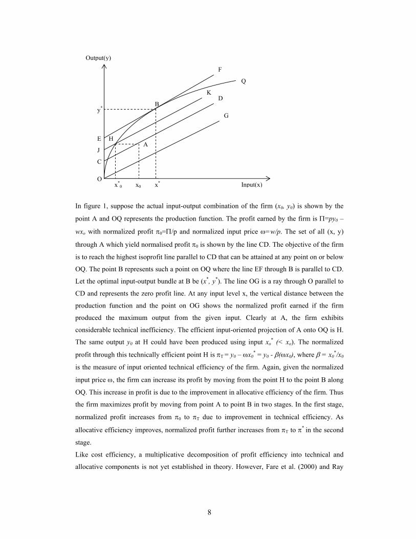
In figure 1, suppose the actual input-output combination of the firm (x0, y0) is shown by the
point A and OQ represents the production function. The profit earned by the firm is Π=py0 –
wxo with normalized profit π0=Π/p and normalized input price ω=w/p. The set of all (x, y)
through A which yield normalised profit π0 is shown by the line CD. The objective of the firm
is to reach the highest isoprofit line parallel to CD that can be attained at any point on or below
OQ. The point B represents such a point on OQ where the line EF through B is parallel to CD.
Let the optimal input-output bundle at B be (x*, y*). The line OG is a ray through O parallel to
CD and represents the zero profit line. At any input level x, the vertical distance between the
production function and the point on OG shows the normalized profit earned if the firm
produced the maximum output from the given input. Clearly at A, the firm exhibits
considerable technical inefficiency. The efficient input-oriented projection of A onto OQ is H.
The same output y0 at H could have been produced using input xo* (< xo). The normalized
profit through this technically efficient point H is πT = y0 – ωx0* = y0 - β(ωx0), where β = x0
*/x0
is the measure of input oriented technical efficiency of the firm. Again, given the normalized
input price ω, the firm can increase its profit by moving from the point H to the point B along
OQ. This increase in profit is due to the improvement in allocative efficiency of the firm. Thus
the firm maximizes profit by moving from point A to point B in two stages. In the first stage,
normalized profit increases from π0 to πT due to improvement in technical efficiency. As
allocative efficiency improves, normalized profit further increases from πT to π* in the second
stage.
Like cost efficiency, a multiplicative decomposition of profit efficiency into technical and
allocative components is not yet established in theory. However, Fare et al. (2000) and Ray
x*0 x0 x*
A
B
G
D K
Q
F
E
J
C
O
y*
H
Input(x)
Output(y)

9
(2004) provided an alternative additive decomposition of profit efficiency. For multiple-input,
multiple-output case, define:
Δ = Π* - Π0 = (ΠT - Π0) + (Π* - ΠT)
⇒ δ = Δ/C0 = (ΠT - Π0)/C0 + (Π* - ΠT)/C0,
where, C0 is the actual cost of the firm with input-output bundle (x0, y0). Here δ represents the
lost or unrealized part of the maximum return on outlay. The first component of δ is δT =
)1(/)]()[( 00000 ββ −=′′−′−′−′ xwxwypxwyp = input oriented technical inefficiency of
the bank. The other component δA = 00*0* /)]()([ xwxxwyyp ′−′−−′ β denotes the return
on outlay lost due to allocative inefficiency. As β lies between 0 and 1, δT also lies between 0
and 1. But δA (≥0) can actually exceed 1 and thus normalized difference measure of profit
inefficiency can also exceed 1.
3.3 Univariate analysis and determinants of inefficiency Multivariate approach: a Tobit analysis
In order to examine the sources of efficiency, efficiency estimates derived in the first stage
DEA are regressed on several bank attributes. The primary goal of the second-stage analysis is
to test various hypotheses on how efficiency is related to these factors by treating them as
potential correlates of efficiency. Several hypotheses are postulated in the literature, mostly
dealing with ownership, size, corporate governance, market power, risk, balance sheet
composition and age.
A commonly held view in the efficiency literature is that the use of Tobit model can handle the
characteristics of the distribution of efficiency measures and thus can provide important policy
guidelines (De Young and Hassan, 1998). As the estimated value of profit efficiency score
(dependent variable) is bounded between 0 and 1, an appropriate theoretical specification is a
Tobit model with two-side censoring. However, banks with efficiency score of 0 will never be
observed in practice. Therefore, the results of the empirical analysis will not be different if one
specifies a one or a two-sided Tobit model. Accordingly, DEA profit efficiency scores
obtained in the first stage are used as the dependent variables in the second stage one-side
censored Tobit model in order to allow for the restricted (0, 1] range of efficiency values.6 The
standard Tobit model can be defined as follows:
00/*
0 εβ += xy
*00 yy = if 0*
0 >y , and 0, otherwise (6)
6 Profit efficiency, by definition, can be negative. However, our empirical estimates of profit efficiency of individual banks consistently fell within (0, 1] throughout 1992-2004.

10
where, x0 is a vector of explanatory variables and β is the set of parameters to be estimated.
),0(~ 20 σε N denotes the error term. The *
0y is a latent variable and 0y is the profit
efficiency score obtained from the first stage DEA models.
Using the profit efficiency scores as the dependent variable, we estimate the following
regression model:
Θjt = β0+ ∑=
04
93_
kk kYRβ +β1SIZEjt+β2LISTINGjt+β3DEP_SIjt+β4PRO_DIVjt+β5AGEjt+
β6PUBLICjt+β7PRIVATEjt+β8(PRIVATE*AGE)jt+β9TERM_Djt+β10CURRENT_Djt+ β11LOANjt+β12LIQUIDITYjt+β13AST_Gjt+β14NNPAjt+β15CRARjt+β16RWAjt+ εjt
(7) Where, Θjt is the profit efficiency of the jth bank in period ‘t’ obtained from the
DEA model. The independent variables capture the various facets of banking activity. On the liability side,
we include three variables: the share of deposits in total deposits (DEP_SI) as a proxy
indicator of individual bank’s market control. If concentration leads to higher prices and
profits, then we expect a positive coefficient. Second, we include the proportion of term
deposits to total deposits (TERM_D). A large share of term deposits in total deposits in an
environment of falling interest rates is expected to lead to higher cost and, therefore, we expect
a negative coefficient of this variable. Berger and Mester (2003) report that banks those rely
more on purchased funds (core deposits) tend to have lower profit efficiencies. Third, we
include the proportion of current deposits to total deposits (CURRENT_D) in order to
ascertain the effect of heterogeneity in liability structure on efficiency.
Two variables are included on the asset side. The loan ratio (LOAN), defined as the ratio of
loans to total assets, takes into consideration the most risky bank asset. An increase in the loan
ratio implies a higher risk profile of the bank balance sheet and therefore, a rise in risk-
weighted assets. To the extent that such credit extension is accompanied by prudent risk
management practices, this is expected to raise interest incomes and consequently, profits.
Besides, higher loan-to-asset ratio might imply higher market power in loan markets. Second,
the proportion of liquid assets to total assets (LIQUIDITY) is included to capture banks' cash
management practices.7 A high proportion of liquid assets could be indicative of poor cash
management which results to low interest income. The coefficient on this variable, is,
therefore, expected to be negative.
We include a variable PRO_DIV to capture the product diversity of the bank. Product diversity
is closely related to scope efficiency, whether a bank is producing the most cost efficient 7 Comprising of cash in hand, balances with the central bank, money at call and short notice and liquid securities.

11
combination of products. Therefore, banks shifting towards producing a broader mix of
services are expected to experience higher profit efficiency.
Among the bank-specific controls, we include bank size (SIZE), defined as logarithm of total
assets. We also include the growth of total assets (ASST_G). While an over-extension of credit
by banks is likely to engender faster asset growth with concomitant rise in profits, on the flip
side, this can lead banks to compromise on their credit risk management practices, leaving
them with higher delinquent loans on their books and lower profitability levels. The sign on
this variable is, therefore, ambiguous. We also focus on the banks' asset quality, soundness and
portfolio risk on the estimated profit efficiency.
Any analysis of efficiency needs to take on board the various macroeconomic, regulatory and
other factors. To address this aspect, we include several dummy variable. First, the dummy
variable (LISTING) equals 1 in the year in which a bank (state-owned or private) made an
equity offering and for all subsequent years thereafter and zero, otherwise (Das, 2002; Ghosh
and Das, 2006). Second, AGE is included as an indicator variable which equals one if the bank
became operational after 1992 and zero otherwise. Third, we include dummies for bank
ownership. Accordingly, we include the variable PUBLIC which equals one for state-owned
banks, else zero. Likewise, a dummy variable PRIVATE equals one if a bank is private, else
zero. The interaction of PRIVATE with AGE is included to ascertain the differential behaviour
of de novo private banks (established post initiation of reforms in 1992) as compared with old
private banks (in existence prior to 1992) on profit efficiency. Finally, we include year
dummies for from 1993 to 2004 (excluding the base year 1992) to account for changes in the
macroeconomic environment and in the regulatory treatment of banks over time.
We estimated 4 variants of the Tobit model (Models 1 to 4) depending on the availability of
data (Table 11). The base model is estimated over the entire period 1992-2004 (Model 1),
while the second model is based on 1993-2004 since one year of observation is lost with the
inclusion of ASST_G as an additional variable (Model 2). Models 3 and 4 sequentially include
the bank soundness and portfolio risk variables, respectively, and are estimated over a shorter
time frame, coinciding with the availability of bank-level data on these variables. The
specified Tobit model in (8) is estimated with heteroscedasticity option using the maximum
likelihood method. Given the unbalanced nature of the panel, we have a maximum of 1111
bank-years (as in Model 1) to a minimum of 575 bank-years, as in Model 4.
6. Empirical Results
The empirical results are classified into three broad heads: first, it describes the estimates of
overall cost and profit efficiency during 1992-2004. Second, it employs a univariate cross-

12
tabulation approach to examine the empirical correlates of cost and profit (in)efficiency across
different ownerships and size classes. This approach, however, does not satisfactorily address
the interrelationship among various efficiency measures and bank financial parameters, since
most bank characteristics would be correlated with each other. Thereafter, a multivariate
regression framework is also employed to relate efficiency scores to bank characteristics.
6.1 Cost and profit efficiency of Indian Banks
Table 3 presents the year-wise distribution of cost and profit efficiency scores. High level of
relative average cost efficiency scores (along with low standard deviation) of Indian banks
illustrates that most of the banks lies close to the benchmark cost frontier. The average cost-
inefficiency of Indian banks was found to be relatively low. In other words, both technical
efficiency (input-oriented) and allocative efficiency (input-oriented) of Indian banks are at a
reasonably high level. In other words, the evidence suggests that these banks are able to
control the underutilization and wastage of valuable input resources and to a great extent
managed to choose proper input-mix as against their competing demands.
Unlike cost efficiency, profit efficiency estimates suggest a large asymmetry among banks.
More specifically, banks appear to lie well inside the efficient profit frontier. For majority of
the years, average profit efficiency was below 50%. In latter half of the sample period, as
profit considerations of banks gained prominence, more number of banks performed relatively
close to the benchmark which resulted in some improvement in profit efficiency, particularly
after 2000. These results are in sharp contrast to the findings of Bauer et al. (1998) who
observed that X-inefficiency is the major source of performance problems among financial
institutions.
[Table 2]
6.2 Univariate approach
Under the univariate approach, the estimates of cost and profit efficiency scores obtained from
the DEA models are cross tabulated and analysed to examine how cost and profit efficiency
varies across ownerships and size classes. As the difference in cost efficiency scores are not
perceptibly large, we restricted our analysis only to profit efficiency scores.
In contrast, average profit efficiency of Indian private banks and foreign banks operating in
India has been much lower than that of state-owned banks. In particular, there is no clear
evidence of relative improvement of profit efficiency over time for foreign banks. The average
efficiency scores of Indian private banks have moved somewhat erratically over the years but
their performance seems to have improved slowly over the period. In order to further
investigate the difference in profit efficiency scores across ownerships, we perform Kruskal-
Wallis’ non-parametric tests separately for individual years. The results indicate that, in most
of the years, the average efficiency scores between various bank groups are significantly

13
different. Efficiency estimates of public sector banks are significantly higher than Indian
private or foreign banks. Significant efficiency differential between Indian private and foreign
banks also underscored the need for separate treatment in designing specific policy guidelines
within the private sector.
The relationship between profit efficiency and bank size is presented in Table 3.8 Both the big
and large banks recorded relatively high efficiency scores; profit inefficiency was persistent
primarily for small banks. These results indicate that except for the small banks, across all
other size categories, banks moved progressively closer to the profit frontier and this trend
gathered momentum during the latter half of the sample period. It is, therefore, clear that the
banks in India can increase their profit performance significantly merely by adopting the best
practices within their peer size groups. Low level of efficiency among the banks in the
smallest size class indicates that with the existing scale of operations, these banks are
operating far below the efficient frontier. On the other hand, big and large banks do not appear
to exhibit major size related cost disadvantage compared to small banks.
[Table 3] 6.3 Decomposition of profit efficiency
Following from the earlier discussion, a simple additive decomposition of profit efficiency is
presented in Table 6. It is observed that the loss or unrealized part of the maximum return on
outlay (δ) has been declining over time. On the other hand, commercial banks are losing very
little profit due to their (input-oriented) technical inefficiency. For most of the years after
deregulation, technical inefficiency remained small around 5%. On the contrary, a large
portion of return on outlay lost is emanating from the high levels of allocative inefficiency.
Dimensionally, allocative inefficiency alone accounted for more than 85% return on outlay
lost and such phenomenon is fairly persistent even after a decade of deregulation.
Traditionally, banks in India support the government borrowing programs by way of large
investments in government securities. In addition, strict capital regulations also instigated
Indian banks to divert resources from conventional lending to risk-free government securities.
Therefore, as competition intensifies, banks will need to undertake pro-active measures to
further improve their efficiency.
The results of the multivariate regressions are set out in Table 4. In Model 1, the positive and
statistically significant coefficient on SIZE is consistent with the fact that larger banks are
better able to reach their optimal mix and scale of outputs and hence raise their profit
efficiency. Second, the coefficient on DEP_SI is positive and statistically significant. Banks in
8 Following Mohan (2006), four size classes have been considered. These are: I-small: Assets up to Rs.50 billion, II-medium: Assets between Rs.50 billion to Rs.100 billion, III-big: Assets between Rs.100 billion to Rs.200 billion, IV-large: Assets above Rs.200 billion.

14
less competitive markets can charge higher prices for their services and eventually make
supernormal profits. Empirical results for the U.S. banking industry also confirm a similar
phenomenon (Stiroh and Starhan, 2003). As markets become more open, the link between
performance and market share intensifies. Over time, these competitive dynamics reallocated
control of the banking industry toward the better-run banks. Third, the coefficient of AGE is
observed to be negative and statistically significant. Age effect on profit efficiency of these
banks, as captured by PRIVATE*AGE, has been positive and statistically significant.
The empirical evidence strongly supports the claim that banks with greater reliance on term
deposits (TERM_D) are less profit efficient. Typically, private and foreign banks finance their
business expansion with expensive term deposits. In fact, the coefficient of term deposits was
found to be negative and statistically significant in 3 out of the 4 models. Therefore, high input
cost is a key determinant of low profit efficiency of the Indian banking sector. The positive
coefficient on the LOAN variable provides support to the efficient structure hypothesis: due to
their ability to manage operations more productively, relatively efficient banks might have
lower production cost, which enables them to offer more loan on more competitive terms and
ultimately garner larger market shares.
The results indicate a positive coefficient of size and it is statistically significant when the
selected models control for asset quality and risk exposure. The larger banks might be better
able to reach their optimal mix and scale of outputs and hence increasing profit efficiency.
Besides, larger banks might become efficient simply by virtue of their ability to achieve
optimal output, i.e., large banks may have higher profits for a given set of prices primarily
because they were able to gain size over a period.
In the second model (Model 2), the coefficient on the asset growth variable is estimated to be
positive and statistically significant. If banks asset base expand depending on the growth in
demand for banking services, this greater demand might provide more opportunities to make
profits in the short run. Thus, our results confirm the existence of external factors shaping the
profitability of banks.
The third model includes the bank soundness (CRAR) and asset quality (NNPA) variables.
Clearly, banks with higher regulatory capital were observed to be more profit efficient. One
possible reason might be that efficient banks generate higher profits, which might lead to
higher capital as a result of high reserve accumulation. Evidence for the US banking industry
is also supportive of this fact (Kwan and Eisenbis, 1997).
In the final specification (Model 4), it is observed that banks with greater portfolio risk (RWA)
exhibit lower profit efficiency. This finding concurs with the ‘bad management hypothesis’
(Berger and DeYoung, 1997). In other words, low profit efficiency is a manifestation of
inadequate loan monitoring and control practices, a factor that is typically associated with
subpar management quality.

15
Summing up, the evidence indicates that, large, listed banks with a bigger loan portfolio
exhibit greater profit efficiency. Furthermore, well-capitalized and well-managed banks are
able to generate higher profits. And finally, state-owned banks have been able to successfully
withstand the competitive pressures from their private and foreign counterparts and in fact,
their profit efficiency was observed to be higher than the private players.
7. Conclusion
Financial sector reforms in India, initiated about one and a half decades ago, have strengthened
the health of financial intermediaries, deepened financial markets and enhanced the
instruments available in the financial system. Notwithstanding these salutary developments,
there is enough scope for further improvements of the performance of banks. In comparison
with international standards, Indian banks would need to improve their technological
orientation and expand the possibilities for augmenting their financial activities in order to
improve their profit efficiency in the near future.

16
References Ahluwalia M.S. (2002): “Economic Reforms in India Since 1991: Has Gradualism Worked?”, Journal of Economic Perspectives, 16, 67-88. Akhigbe, A. and J.E. McNulty (2003): “The profit efficiency of small US commercial banks”, Journal of Banking and Finance, 27, 307–325. Amel, D., C. Barnes, F. Panetta and C. Salleo (2004): “Consolidation and efficiency in the financial sector: A review of the international evidence,” Journal of Banking and Finance, 28, 2493-2519. Banker, R.D., A. Charnes and W. W. Cooper (1984): “Some Models for Estimating Technical and Scale Inefficiencies in Data Envelopment Analysis”, Management Science, 30, 1078-1092. Barr, R.S., K.A. Killgo, T.F. Siems and S. Zimmel (2000): “Evaluating the Productive Efficiency and Performance of U.S. Commercial Banks”, Managerial Finance, 28, 3-25. Bauer, P.W., A.N. Berger, G.D. Ferrier and D.B. Humphrey (1998): “Consistency conditions for Regulatory Analysis of Financial Institutions: A Comparison of Frontier Efficiency Methods”, Journal of Economics and Business, 50, 85-114. Berger, A.N. and L.J. Mester (2003): "Explaining the dramatic changes in performance of US banks: technological change, deregulation, and dynamic changes in competition," Journal of Financial Intermediation, 12, 57-95. Berger, A.N., D.B. Humphrey (1992), “Measurement and efficiency issues in commercial banking” in Z. Griliches (ed.), Output Measurement in the Service Sector, National Bureau of Economic Research, Studies in Income and Wealth, University of Chicago Press, IL, 245-279. Berger, A.N. and D.B. Humphrey (1997): “Efficiency of Financial Institutions: International Survey and Directions for Future Research”, European Journal of Operations Research, 98, 175-212. Bhattacharyya, A., C.A.K. Lovell and P. Sahay (1997): “The Impact of Liberalisation on the Productive Efficiency of Indian Commercial Banks”, European Journal of Operations Research, 98, 332-345. Bonin, J.P., I. Hassan and P. Wachtel (2005): Bank performance, efficiency and ownership in transition countries, Journal of Banking and Finance, 29, 31–53. Chatterjee, G. (2006): “Is Efficiency of Banks in India a Cause for Concern? Evidence from Post-reform Era”, forthcoming, Journal of Emerging Market Finance. Charnes, A., W.W. Cooper and E. Rhodes (1978): “Measuring the Efficiency of Decision Making Units”, European Journal of Operations Research, 2, 429-444. Clark, J.A. and T.F. Siems (2002): “X-Efficiency in Banking: Looking beyond the Balance Sheet”, Journal of Money, Credit, and Banking, 34, 987-1013. Das, Abhiman (1997): “Technical, Allocative and Scale Efficiency of Public Sector Banks in India”, Reserve Bank of India Occasional Papers, June-September, 18, 279-301.

17
Das, Abhiman, A.K. Nag and S.C. Ray (2005): “Liberalization, Ownership and Efficiency in Indian Banking”, Economic and Political Weekly, 40, 1190-1197. Gilbert, R.A. and P.W. Wilson (1998): “Effects of Deregulation on the Productivity of Korean Banks”, Journal of Economics and Business, 50, 133-155. Government of India (1991): Report of the Committee on the Financial System, Government of India: New Delhi. Government of India (1998): Report of the Committee on Banking Sector Reforms, Government of India: New Delhi. Hao, J, C.W. Hunter and W.K. Yang (2001): “Deregulation and Efficiency: The Case of Private Korean Banks”, Journal of Economics and Business, 53, 237-254.
Ishik I. and M. K. Hassan (2003): Efficiency, Ownership and Market Structure, Corporate Control and Governance in the Turkish Banking Industry” Journal of Business Finance and Accounting, 30, 1363-1421.
Jalan, B. (2002). ‘Indian Banking and Finance: Managing New Challenges’, Speech delivered at the Bank Economists’ Conference, Kolkata, January 14. Karim, M.Z.A. (2001): “Comparative bank efficiency across select ASEAN countries”, ASEAN Economic Bulletin, 18, 289-304. Kawn S.H. (2003): Operating performance of banks among Asian economies: An international and time series comparison, Journal of Banking and Finance 27, 471–489. Kumbhakar, S. C. and S. Sarkar (2005): “Deregulation, Ownership and Efficiency Change in Indian Banking: An application of Stochastic Frontier Analysis”, in Theory and Application of Productivity and Efficiency, Econometric and DEA Approach, Ghosh, R. and C. Neogi, eds., Macmillan, India. Kumbhakar, S. C. and S. Sarkar (2003): “Deregulation, Ownership and Productivity Growth in the Banking Industry: Evidence from India”, Journal of Money, Credit, and Banking, 35, 403-414. Leightner, E.J and C.A.K. Lovell (1998): “The Impact of Financial Liberalization on the Performance of Thai Banks”, Journal of Economics and Business, 50, 115-132. Mohan, R. (2006): “Reforms, Productivity and Efficiency in Banking: The Indian Experience”, Address delivered at the Conference of the Pakistan Society of Development Economicts, Islamabad. Available at <www.rbi. org.in> Rammohan, T.T. (2002): “Deregulation and Performance of Public Sector Banks”, Economic and Political Weekly, 37, 393-397. Rammohan, T.T. (2003): “Long-Run Performance of Public and Private Sector Bank Stocks”, Economic and Political Weekly, 38, 785-788. Rammohan, T.T. and S.C. Ray (2004): “Comparing Performance of Public and Private Sector Banks: A Revenue Maximisation Efficiency Approach”, Economic and Political Weekly, 39, 1271-1276.
18
Reddy Y.V. (2002): “Public Sector Banks and the Governance Challenge: Indian Experience”, Lecture delivered at the World Bank, IMF and Brookings Institutions Conference. Reserve Bank of India (1954): All India Rural Credit Survey Committee, Mumbai. Reserve Bank of India: Statistical Tables Relating to Banks in India (various years), RBI: Mumbai. Sarkar, J., S. Sarkar, and S.K. Bhaumik (1998): “Does Ownership Always Matter? Evidence from the Indian Banking Industry”, Journal of Comparative Economics, 26, 262-281. Shanmugam, K.R. and Abhiman Das (2004): Efficiency of Indian Commercial Banks during Reform Period, Applied Financial Economics, 14, 681-686. Shyu, J. (1998): “Deregulation and Bank Operating Efficiency: An Empirical Study of Taiwan Banks”, Journal of Emerging Markets, 3, 27-46. Stiroh, K (2004): “Diversification in Banking: Is Noninterest Income the Answer?” Journal of Money, Credit, and Banking, 36, 853-882. Stiroh, K. and P.E. Strahan (2003): “Competitive Dynamics of Deregulation: Evidence from U.S. Banking”, Journal of Money, Credit, and Banking, 35, 801-828. Vander Vennet, R (2002): “Cost and Profit Efficiency of Financial Conglomerates and Universal Banks in Europe”, Journal of Money, Credit, and Banking, 34, 254-282. Williams J. and N. Nguyen (2005): “Financial liberalisation, crisis, and restructuring: A comparative study of bank performance and bank governance in South East Asia”, Journal of Banking and Finance, 29, 2119–2154.

19
Table 1: Summary Statistics of Inputs, Outputs and Prices
(Amount in Rs. billion) Year/variables 1992 1998 2004
Mean Std. Dev.
Mean Std. Dev.
Mean Std. Dev.
Inputs xd Deposits 36.45 80.70 68.84 156.49 186.11 389.10 xl Labour – No. of employees 12912 29328 10352 27728 10088 24742 xk Capital – fixed assets 0.27 0.55 1.34 2.26 2.50 5.47xq Quasi-fixed inputs - equity 1.23 2.29 5.69 11.61 13.71 25.82 Input prices wd Price of deposits 0.0635 0.0113 0.0769 0.0258 0.0480 0.0159 wl Price of labour 0.0084 0.0051 0.0287 0.0258 0.0517 0.0648wk Price of capital 0.0077 0.0064 0.0049 0.0050 0.0075 0.0088 Outputs
y1 Loans and advances 22.01 56.54 34.65 84.94 102.32 203.13 y2 Investments 13.54 30.45 29.06 65.18 94.80 218.89 y3 Other income 0.65 1.72 1.29 3.12 4.70 9.49 Output prices p1 Price of loans and advances 0.1551 0.0819 0.1349 0.0365 0.0935 0.0464 p2 Price of investments 0.0895 0.0132 0.1084 0.0262 0.0814 0.0216 Cost 2.59 6.00 5.01 11.29 9.23 21.32 Revenue 4.80 11.70 8.61 19.57 20.78 42.64 Profit 2.22 5.82 3.59 8.35 11.56 21.92 All nominal variables have been deflated by the Wholesale price Index (Base 1993-94=100)

20
Table 2: Cost and Profit Efficiency of Domestic Indian banks
Year No. of banks
Cost efficiency Profit efficiency Mean Std.
Dev. Mean Std.
Dev. 1992 51 0.9072 0.0854 0.5049 0.2338 1993 51 0.8754 0.0911 0.4258 0.2361 1994 51 0.9124 0.0811 0.4275 0.2586 1995 51 0.9191 0.0647 0.4004 0.2466 1996 61 0.9047 0.0894 0.4591 0.2603 1997 59 0.9418 0.0656 0.4880 0.2494 1998 59 0.9606 0.0480 0.5615 0.2337 1999 58 0.9267 0.0748 0.5975 0.2347 2000 59 0.9546 0.0679 0.6382 0.2285 2001 58 0.9370 0.0673 0.6270 0.2331 2002 57 0.8566 0.1243 0.6503 0.2189 2003 56 0.8621 0.1237 0.6624 0.2144 2004 55 0.8921 0.1122 0.7063 0.2066
Note: Domestic Indian banks refers to includes state-owned and private banks
Table 3: Size and Profit Efficiency of Indian banks Year/Size I-Small II-Medium III-Big IV-Large
Mean Std.
Dev. Mean Std.
Dev.Mean Std.
Dev.Mean Std.
Dev.1992 0.2726 0.2395 0.2583 0.0971 0.4311 0.2056 0.4170 0.19101993 0.3407 0.2372 0.3568 0.1922 0.4559 0.2767 0.3720 0.2049 1994 0.2505 0.1813 0.3590 0.1399 0.5284 0.2605 0.4717 0.24371995 0.2167 0.1714 0.3295 0.1063 0.5005 0.2878 0.4174 0.2184 1996 0.3878 0.2382 0.4641 0.2169 0.5195 0.2663 0.4369 0.2520 1997 0.3486 0.2656 0.4497 0.1437 0.5213 0.2350 0.5421 0.2627 1998 0.3791 0.2403 0.6103 0.1757 0.6378 0.2288 0.5631 0.2496 1999 0.4183 0.2645 0.5905 0.1946 0.6356 0.2216 0.6524 0.2393 2000 0.3923 0.2541 0.5899 0.1286 0.7220 0.1879 0.6765 0.2494 2001 0.3232 0.2387 0.4713 0.0833 0.6415 0.2253 0.6729 0.2083 2002 0.3224 0.2459 0.5236 0.1138 0.6809 0.2140 0.7120 0.2172 2003 0.3395 0.2529 0.5753 0.1316 0.6872 0.1725 0.7354 0.2049 2004 0.3434 0.2739 0.5910 0.1950 0.7467 0.1633 0.7618 0.1926
* Based on total assets, four size classes have been considered. These are: I: Assets up to Rs.50 billion, II: Assets between Rs.50 billion to Rs.100 billion, III: Assets between Rs.100 billion to Rs.200 billion, IV: Assets above Rs.200 billion.

21
Table 4: Parameter Estimates of Tobit Regression
Parameters Model 1 Model 2 Model 3 Model 4 Intercept 0.1989
(0.1237) 0.1772
(0.1344)0.3610
(0.1565)0.1240
(0.1834) SIZE 0.0320*
(0.0063) 0.0275* (0.0067)
0.0189** (0.0083)
0.0141 (0.0105)
LISTING 0.0147 (0.0175)
0.0225 (0.0182)
0.0395*** (0.0206)
0.0451** (0.0210)
DEP_SI 1.2558* (0.2979)
1.2356* (0.3116)
1.2495* (0.3565)
1.3604* (0.3571)
PRO_DIV -0.0090 (0.0425)
0.0292 (0.0453)
0.0029 (0.0486)
0.0786 (0.0639)
AGE -0.1344* (0.0222)
-0.1369* (0.0235)
-0.1136* (0.0273)
-0.0500 (0.0436)
PUBLIC 0.0366 (0.0313)
0.0613*** (0.0326)
0.0831** (0.0370)
0.0461 (0.0428)
PRIVATE 0.0144 (0.0262)
0.0213 (0.0272)
0.0057 (0.0297)
-0.0604*** (0.0356)
PRIV_AGE 0.1165* (0.0311)
0.1228* (0.0327)
0.1271* (0.0370)
0.0630 (0.0497)
TERM_D -0.3478* (0.1018)
-0.3388* (0.1088)
-0.2697** (0.1221)
-0.0837 (0.1463)
DEMAND_D -0.1725 (0.1145)
-0.1366 (0.1236)
0.0381 (0.1413)
0.1852 (0.1980)
LOAN 0.3722* (0.0815)
0.4154* (0.0880)
0.2708* (0.0944)
0.8914* (0.1334)
LIQUIDITY -0.0637 (0.0866)
-0.0554 (0.0933)
-0.0868 (0.1007)
0.0538 (0.1483)
AST_G
0.0004** (0.0002)
0.0003** (0.0002)
0.0001 (0.0002)
NNPA
-0.0013 (0.0010)
-0.0001 (0.0016)
CRAR
0.0023* (0.0004)
0.0051* (0.0010)
RWA
-0.3240* (0.0758)
Year dummies YES YES YES YES N 1111 1008 788 575 Log Likelihood 197.9018 183.8397 163.9996 176.9841
Figures in bracket indicate standard errors. ***, ** and * indicate statistical significance at 1, 5 and 10%, respectively