MPRAMunich Personal RePEc Archive

Finite State Markov-ChainApproximations to Highly PersistentProcesses

Karen A. Kopecky and Richard M. H. Suen

University of California, Riverside

8. May 2009

Online at http://mpra.ub.uni-muenchen.de/15122/MPRA Paper No. 15122, posted 9. May 2009 18:03 UTC

Finite State Markov-Chain Approximations to

Highly Persistent Processes�

Karen A. Kopeckyy Richard M. H. Suenz

May 2009

Abstract

This paper re-examines the Rouwenhorst method of approximating �rst-order autore-

gressive processes. This method is appealing because it can match the conditional and

unconditional mean, the conditional and unconditional variance and the �rst-order au-

tocorrelation of any AR(1) process. This paper provides the �rst formal proof of this

and other results. When comparing to �ve other methods, the Rouwenhorst method

has the best performance in approximating the business cycle moments generated by the

stochastic growth model. It is shown that, equipped with the Rouwenhorst method, an

alternative approach to generating these moments has a higher degree of accuracy than

the simulation method.

Keywords: Numerical Methods, Finite State Approximations, Optimal Growth Model

JEL classi�cation: C63.

�We thank Russell Cooper and conference participants at the UCR Conference on Business Cycles forhelpful comments and suggestions. We thank Yundong Tu for excellent research assistance.

yDepartment of Economics, Social Science Center, Room 4701, The University of Western Ontario, London,Ontario, N6A 5C2, Canada. Email: kkopecky@uwo.ca.

zCorresponding author. Department of Economics, Sproul Hall, University of California, Riverside CA92521-0427. Email: richard.suen@ucr.edu. Tel.: (951) 827-1502. Fax: (951) 827-5685.

1

1 Introduction

In macroeconomic models, the exogenous stochastic process is typically assumed to follow a

stationary �rst-order autoregressive process. Two well-known examples are the asset pricing

model à la Lucas (1978), and the standard real business cycle (RBC) model. In Lucas�model,

the stochastic dividend stream is assumed to follow a Markov process. In the RBC model, the

logarithm of the productivity shock is assumed to follow a Gaussian AR(1) process. In order

to solve these models numerically, the continuous-valued autoregressive process is usually

approximated by a discrete state-space Markov chain. To this end, researchers typically

employ the approximation method proposed by Tauchen (1986), or the quadrature-based

method developed in Tauchen and Hussey (1991). Although these methods di¤er substantially

in details, the underlying idea is the same, that is to construct a discrete state-space Markov

chain with transition probabilities that provide a good approximation for the conditional

density of the autoregressive process. For AR(1) processes with low persistence, these methods

can generate an accurate approximation even when a very coarse state space is used in the

approximate Markov chain. However, the performance of these methods deteriorates when the

serial correlation is very close to one.1 This particular problem has been examined closely in a

recent study by Flodén (2008). This author shows that the accuracies of the Tauchen (1986)

method and the Tauchen-Hussey method are signi�cantly lowered when the serial correlation

of the underlying process is greater than 0.95. This problem persists even if one signi�cantly

increases the number of states in the discrete state-space Markov chain.

The �ndings in Flodén (2008) raise concerns because macroeconomic studies often employ

highly persistent processes. These �ndings thus call for a more reliable technique to approxi-

mate highly autocorrelated processes. The main objective of this paper is to consider such a

technique. More speci�cally, the current study re-examines a discrete approximation method

�rst proposed in Rouwenhorst (1995) but largely overlooked by the existing literature.2 Sim-

ilar to the aforementioned methods, the Rouwenhorst method is about the construction of an

approximate discrete state-space Markov chain. But unlike the other methods, the transition

1This weakness is acknowledged in the original papers. In Tauchen (1986, p.179), the author notes that�Experimentation showed that the quality of the approximation remains good except when � [the serial cor-relation] is very close to unity.� In Tauchen and Hussey (1991), the authors note that for processes with highpersistence, �adequate approximation requires successively �ner state spaces.�

2An exception is Lkhagvasuren and Galindev (2008) which uses the Rouwenhorst method to approximate�rst-order vector autoregressive processes.

2

probabilities of the approximate Markov chain are not intended to mimic the conditional dis-

tribution of the underlying AR(1) process. This might seem like a weakness at �rst, but the

Rouwenhorst method has a number of desirable features that are not matched by the other

methods. First, only a few parameters are used in constructing the approximate Markov

chain under this method. It is thus much more parsimonious and much easier to implement

than the quadrature-based method developed in Tauchen and Hussey (1991). Second, the

constructed Markov chain can be calibrated to match �ve important statistics of any station-

ary AR(1) process. These are the conditional and unconditional mean, the conditional and

unconditional variance, and the �rst-order autocorrelation. Thus, even though the transition

probabilities of the approximate Markov chain do not mimic the conditional distribution of

the underlying AR(1) process, it can still exactly match the �rst two moments. Third, the

Rouwenhorst method is particularly desirable for approximating Gaussian AR(1) processes.

This is because the invariant distribution of the constructed Markov chain is a binomial dis-

tribution, which converges to the standard normal distribution when the number of states in

the state space is su¢ ciently large.

Some of these features have been mentioned in Rouwenhorst (1995). But a formal proof

of these results is still lacking. It is also unclear whether matching the moments of the

AR(1) process is important in terms of solving dynamic general equilibrium models. In

quantitative studies, obtaining a good approximation for the AR(1) process is seldom an end

in itself. Thus a more appropriate metric for evaluating approximation methods in general

would be their impact on the computed solutions of the general equilibrium models. Very

few attempts have been made to assess the relative performance of the Rouwenhorst method

and other approximation methods on this ground. Thus it remains unclear how the choice of

approximation method would a¤ect the accuracies of the computed solutions in these models.

The current study is intended to �ll these gaps.

The main contribution of this paper is two-fold. First, this paper provides formal proofs

of all the results mentioned above. These results encompass the claims made in Rouwenhorst

(1995). They also extend and generalize those claims in two ways. (i) Rouwenhorst mentions

that when the transition matrix of the approximate Markov chain is symmetric, the invariant

distribution is given by a binomial distribution. The current study shows that the invariant

distribution is binomial even if the symmetric assumption is relaxed. (ii) Rouwenhorst also

3

claims that in the symmetric case, the approximate Markov chain can be calibrated to match

the unconditional mean, the unconditional variance and the �rst-order autocorrelation of

any stationary AR(1) process. This paper shows that the Markov chain can also match the

conditional mean and the conditional variance.

The second contribution of this paper is to compare the Rouwenhorst method to �ve

other approximation methods that are commonly used in the literature. These include the

Tauchen (1986) method, the original quadrature-based method developed in Tauchen and

Hussey (1991), two variations of this method considered in Flodén (2008), and the Adda-

Cooper (2003) method. To achieve this, the prototypical stochastic neoclassical growth model

without leisure is used as the analytical vehicle.3 There are two main reasons why we choose

this particular model. First, the neoclassical growth model is by far the most common analyt-

ical framework in macroeconomics. Variations of the original model have been used to study

a wide range of economic issues. Second, it is possible to derive closed-form solutions for the

neoclassical growth model under certain speci�cations. This property of the model provides

tremendous convenience for evaluating the accuracy of the approximation methods.

The main criterion for evaluating the six approximation methods is the accuracy in ap-

proximating the business cycle moments as predicted by the stochastic growth model. Two

approaches to generating these moments are considered. In the baseline approach, an approx-

imation for the stationary distribution of the state variables is �rst derived. The moments of

interest are then computed directly from this distribution. In the second approach, the busi-

ness cycle moments are generated using the Monte Carlo simulation method. This involves

simulating the model repeatedly using the actual AR(1) process and the computed policy

function, and thus does not require approximating the stationary distribution. One major

di¤erence between these two approaches is the sources of the errors that they introduce. While

both methods su¤er from errors in the computation of the policy function, under the baseline

approach, additional errors arise when approximating the stationary distribution. However,

this approach does not su¤er from the sampling errors that the simulation method generates.

One important �nding of this paper is that, regardless of which approach is taken, the

choice of approximation method can have a large impact on the accuracy of the business

3The same model is used in Taylor and Uhlig (1990) and the companion papers to illustrate and comparedi¤erent solution methods. More recently, Aruoba, Fernández-Villaverde and Rubio-Ramírez (2006) use thesame model, but with labor-leisure choice, to compare di¤erent solution methods.

4

cycle moments computed. Under the baseline approach, the choice of discretization method

has a large impact on the accuracy of the stationary distribution approximation that is used

to compute the moments. In general, a method that generates a good approximation for

the moments of the AR(1) process also tends to yield an accurate approximation for the

stationary distribution. The Rouwenhorst method has the best performance in this regard,

followed by a variation of the quadrature-based method considered in Flodén (2008). In the

sensitivity analysis, it is shown that the superior performance of the Rouwenhorst method is

robust under a wide range of parameter values.

When the Monte Carlo simulation method is used to generate the business cycle moments,

no single method dominates all others in all cases. With a logarithmic utility function and

full depreciation, the six methods yield almost identical results. When a more realistic value

of the depreciation rate is used, the relative performance of the six methods depends on

the number of states in the Markov chain. When a rather coarse state space is used, the

Rouwenhorst method again has the best overall performance. However, when the �neness of

the state space increases, the Adda-Cooper method improves signi�cantly and yields the best

overall performance.

Another important �nding of this paper is that the baseline approach, equipped with the

Rouwenhorst method, has a higher degree of accuracy than the simulation method. This result

is one of interest because the simulation method is considered standard practice in estimating

unknown statistics of stochastic models. Our results, however, show that this is not the most

e¤ective method for generating business cycle moments in the neoclassical growth model.

The rest of this paper is organized as follows. Section 2 presents the Rouwenhorst method.

Section 3 presents the analytical results pertaining to this method. Section 4 presents the

numerical results. Section 5 concludes.

2 The Rouwenhorst Method

Consider the following AR(1) process

zt = �zt�1 + "t; (1)

5

where "t is a white noise with variance �2": If j�j < 1, then the AR(1) process is stationary

and the random variable zt has a mean of zero, a variance of

�2z =�2"

1� �2 ; (2)

and autocorrelations given by

�s =E (ztzt�s)

var (zt)= �s; for s = 0; 1; 2; ::::

If, in addition, "t is normally distributed in each time period, then zt is also normally distrib-

uted.

Rouwenhorst (1995) proposes a discrete approximation to the AR(1) process in (1). This

involves constructing an N -state Markov chain characterized by (i) a symmetric and evenly-

spaced state space YN = fy1; :::; yNg ; with y1 = � and yN = ; and (ii) a transition matrix

�N : For any N � 2; the transition matrix is determined by two parameters, p; q 2 (0; 1) ; and

is de�ned recursively as follows:

Step 1: When N = 2; de�ne �2 as

�2 =

264 p 1� p

1� q q

375 :Step 2: For N � 3; �rst construct the N -by-N matrix

p

264 �N�1 0

00 0

375+ (1� p)264 0 �N�1

0 00

375+(1� q)

264 00 0

�N�1 0

375+ q264 0 00

0 �N�1

375 ; (3)

where 0 is a (N � 1)-by-1 column vector of zeros.

Step 3: Divide all but the top and bottom rows by two so that the elements in each row

sum to one.

6

Rouwenhorst mentions two important attributes of this Markov chain. First, for any

N � 2; the �rst-order autocorrelation is always given by p+ q � 1: Second, in the symmetric

case where p = q; the invariant distribution of �N is a binomial distribution with parameters

N �1 and 1=2: Formally, let � = (�1; :::; �N ) be the invariant distribution of �N :When p = q

holds, the elements in � are given by

�i =

�N�1i�1�

2N�1; for i = 1; 2; :::; N:

It follows that the unconditional mean of the Markov process is zero and the unconditional

variance is

�2y = 2

N � 1 :

These properties are particularly useful when it comes to approximating Gaussian AR(1)

processes. First, the �rst-order autocorrelation of the original AR(1) process (�) and its

variance��2z�can be perfectly matched by setting

=p(N � 1)�z and p = q =

1 + �

2:

Second, since the invariant distribution is a binomial distribution, it is a close approximation

for the standard normal distribution when N is su¢ ciently large. This feature is desirable

because for a Gaussian AR(1) process fztg ; the invariant distribution of the standardized

process fzt=�zg is the standard normal distribution. Thus, the invariant distribution of the

process fyt=�yg can be made arbitrarily close to the invariant distribution of fzt=�zg by

increasing the number of grid points, N:

3 Analytical Results

The objective of this section is to derive and generalize the results mentioned in the previous

section. One problem with the Rouwenhorst method is that the matrix �N generated by the

three-step procedure is very di¢ cult to work with analytically. For this reason, this section

begins by o¤ering a new and simpler procedure for generating the Rouwenhorst matrix. Using

this new procedure, it is shown that a Markov chain with state space YN and transition

7

matrix �N has a unique invariant distribution in the form of a binomial distribution. Unlike

Rouwenhorst (1995), which only considers the case when p = q; the current study shows

that the invariant distribution is binomial for any p; q 2 (0; 1) : The result reported in here

thus encompasses the symmetric case as a special case. Once the invariant distribution is

determined, it is used to derive a set of conditional and unconditional moments for the Markov

chain.

3.1 Reconstructing the Rouwenhorst Matrix

For any p; q 2 (0; 1) ; and for any integer N � 2; de�ne a system of polynomials as follows

� (t;N; i) � [p+ (1� p) t]N�i (1� q + qt)i�1 ; (4)

for i = 1; 2; :::; N: The polynomials in (4) can be expanded to become

� (t;N; i) =

NXj=1

�(N)i;j t

j�1; for i = 1; 2; :::; N: (5)

De�ne an N -by-N matrix �N =h�(N)i;j

iusing the coe¢ cients in (5). Using the generating

function in (4), one can derive the elements in �N recursively using the elements in �N�1; for

N �1 � 2: The details of this procedure are described in Appendix A. The main result of this

subsection is Proposition 1 which states that the matrix �N is identical to the Rouwenhorst

matrix �N for any integer N � 2: Before proceeding to the main result, let�s consider a couple

of simple examples.

For N = 2; the system of polynomials in (4) can be expressed as

264 � (t; 2; 1)� (t; 2; 2)

375 =264 p 1� p

1� q q

375| {z }

�2

264 1t

375 :

Obviously �2 is identical to the Rouwenhorst matrix �2: ForN = 3; the system of polynomials

8

is 266664� (t; 3; 1)

� (t; 3; 2)

� (t; 3; 3)

377775 =266664

p2 2p (1� p) (1� p)2

p (1� q) pq + (1� p) (1� q) q (1� p)

(1� q)2 2q (1� q) q2

377775| {z }

�3

2666641

t

t2

377775 :

Again �3 is identical to the Rouwenhorst matrix �3 (see Rouwenhorst, 1995, p.327). The

general result is established in Proposition 1. All proofs can be found in Appendix B.

Proposition 1 For any N � 2; and for any p; q 2 (0; 1) ; the matrix �N de�ned above is

identical to the Rouwenhorst matrix �N generated by Steps 1-3.

The next result states that �N is a stochastic matrix with non-zero entries. To begin

with, set t = 1 in both (4) and (5) to obtain

NXj=1

�(N)i;j = 1; for i = 1; 2; :::; N:

This means the elements in any row of �N sum to one. If, in addition, �(N)i;j � 0 for all i and

j, then �N is a stochastic matrix. This is proved in the following lemma.

Lemma 2 For any N � 2; the matrix �N de�ned above is a stochastic matrix with no zero

entries.

3.2 Discrete State-Space Markov Chain

Consider a Markov chain with a symmetric and evenly-spaced state space YN = fy1; :::; yNg

de�ned over the interval [� ; ] : In other words, the elements in the state space are given by

yi = � +2

N � 1 (i� 1) ; for i = 1; 2; :::; N:

The transition matrix of the Markov chain is given by �N =h�(N)i;j

ias de�ned above. The

following result follows immediately from Lemma 2.

Proposition 3 For any N � 2; the Markov chain with state space YN = fy1; :::; yNg and

transition matrix �N has a unique invariant distribution �(N) =��(N)1 ; :::; �

(N)N

�, where

9

�(N)i � 0 and

PNi=1 �

(N)i = 1:

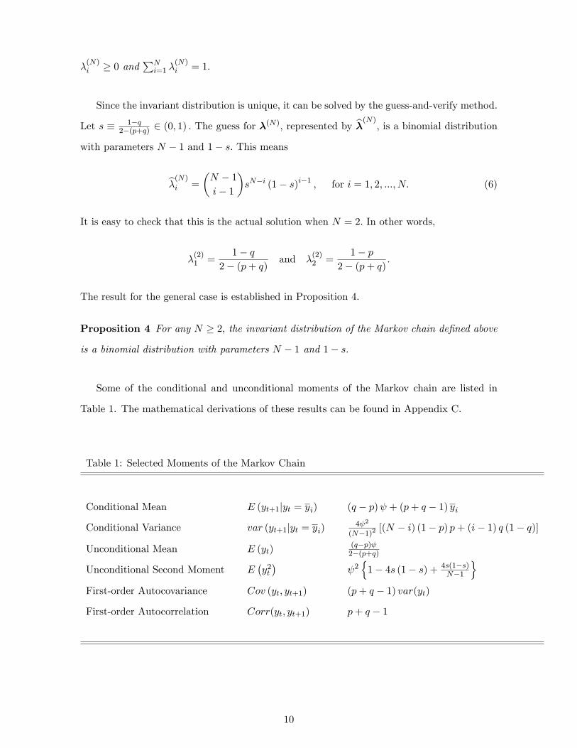
Since the invariant distribution is unique, it can be solved by the guess-and-verify method.

Let s � 1�q2�(p+q) 2 (0; 1) : The guess for �

(N); represented by b�(N); is a binomial distributionwith parameters N � 1 and 1� s: This means

b�(N)i =

�N � 1i� 1

�sN�i (1� s)i�1 ; for i = 1; 2; :::; N: (6)

It is easy to check that this is the actual solution when N = 2: In other words,

�(2)1 =

1� q2� (p+ q) and �

(2)2 =

1� p2� (p+ q) :

The result for the general case is established in Proposition 4.

Proposition 4 For any N � 2; the invariant distribution of the Markov chain de�ned above

is a binomial distribution with parameters N � 1 and 1� s:

Some of the conditional and unconditional moments of the Markov chain are listed in

Table 1. The mathematical derivations of these results can be found in Appendix C.

Table 1: Selected Moments of the Markov Chain

Conditional Mean E (yt+1jyt = yi) (q � p) + (p+ q � 1) yi

Conditional Variance var (yt+1jyt = yi)4 2

(N�1)2 [(N � i) (1� p) p+ (i� 1) q (1� q)]

Unconditional Mean E (yt)(q�p) 2�(p+q)

Unconditional Second Moment E�y2t�

2n1� 4s (1� s) + 4s(1�s)

N�1

oFirst-order Autocovariance Cov (yt; yt+1) (p+ q � 1) var(yt)

First-order Autocorrelation Corr(yt; yt+1) p+ q � 1

10

3.3 Approximating AR(1) Processes

The task at hand is to approximate a given stationary AR(1) process with an N -state Markov

chain. Let fztg be a stationary AR(1) process as de�ned in (1). The random disturbance

term "t is assumed to follow an i.i.d. process with �nite variance �2": As mentioned above, the

unconditional mean of zt is zero, the unconditional variance is given by (2) and the �rst-order

autocorrelation is �: Conditional on the realization of zt�1; the mean and variance of zt are

given by

E (ztjzt�1) = �zt�1 and var (ztjzt�1) = �2":

Next, de�ne an N -state discrete Markov process fytg as in section 3.2 with the following

restrictions imposed:

p = q =1 + �

2and =

pN � 1�": (7)

Using the equations listed on Table 1, it is immediate to see that the resulting Markov chain

fytg has the same unconditional mean, unconditional variance and �rst-order autocorrelation

as fztg : Suppose yt = yi for some t � 0 and for some yi in the state space YN : The conditional

mean and conditional variance of yt+1 are given by

E (yt+1jyt = yi) = �yi and var (yt+1jyt = yi) = �2":

Thus the Markov chain fytg has the same conditional mean and conditional variance as the

AR(1) process fztg :

Two remarks regarding this procedure are worth mentioning. First, under the Rouwen-

horst method, the approximate Markov chain is constructed using � and �2" alone. In particu-

lar, the transition matrix �N is not a discretized version of the conditional distribution of zt:

This is the fundamental di¤erence between this method and the ones proposed by Tauchen

(1986) and Tauchen and Hussey (1991). Second, the above procedure can be applied to any

stationary AR(1) process, including those with very high persistence. Thus, unlike the other

two methods, the one proposed by Rouwenhorst can always match the unconditional variance

and the �rst-order autocorrelation of zt:

Suppose now the random disturbances term "t in the AR(1) process is also normally

11

distributed in each time period t: Then the distribution of zt is a normal distribution. In this

case, the invariant distribution of the Markov chain fytg can provide a good approximation for

the distribution of zt: As shown in Proposition 4, the invariant distribution of yt is always given

by a binomial distribution. Under (7), the mean and variance of the invariant distribution

are zero and �2 � �2"=�1� �2

�, respectively. Thus the standardized process fyt=�g would

converge to the standard normal distribution when N is made su¢ ciently large. According

to the Berry-Esséen Theorem, the rate of convergence is on the order of N�1=2:

4 Stochastic Neoclassical Growth Model

Consider the planner�s problem in the stochastic neoclassical growth model,

maxfCt;Kt+1g1t=0

E0

" 1Xt=0

�tU (Ct)

#

subject to

Ct +Kt+1 = AtK�t + (1� �)Kt;

Ct;Kt+1 � 0;

where Ct denotes consumption at time t; Kt denotes capital and At is the stochastic techno-

logical factor. The function U (�) is the per-period utility function. The parameter � 2 (0; 1)

is the subjective discount factor, � 2 (0; 1) is the share of capital income in total output

and � 2 (0; 1] is the depreciation rate of capital. The logarithm of the technological shock,

represented by at � lnAt; is assumed to follow an AR(1) process,

at+1 = �at + "t+1; (8)

where "t+1 � i.i.d. N�0; �2"

�and � 2 (0; 1) : Conditional on at = a; the random variable

at+1 is normally distributed with mean �a and variance �2": Let F (�ja) be the conditional

distribution function. For any given value of a, de�ne K (a) by

K (a) =

�exp (a)

�

� 11��

:

12

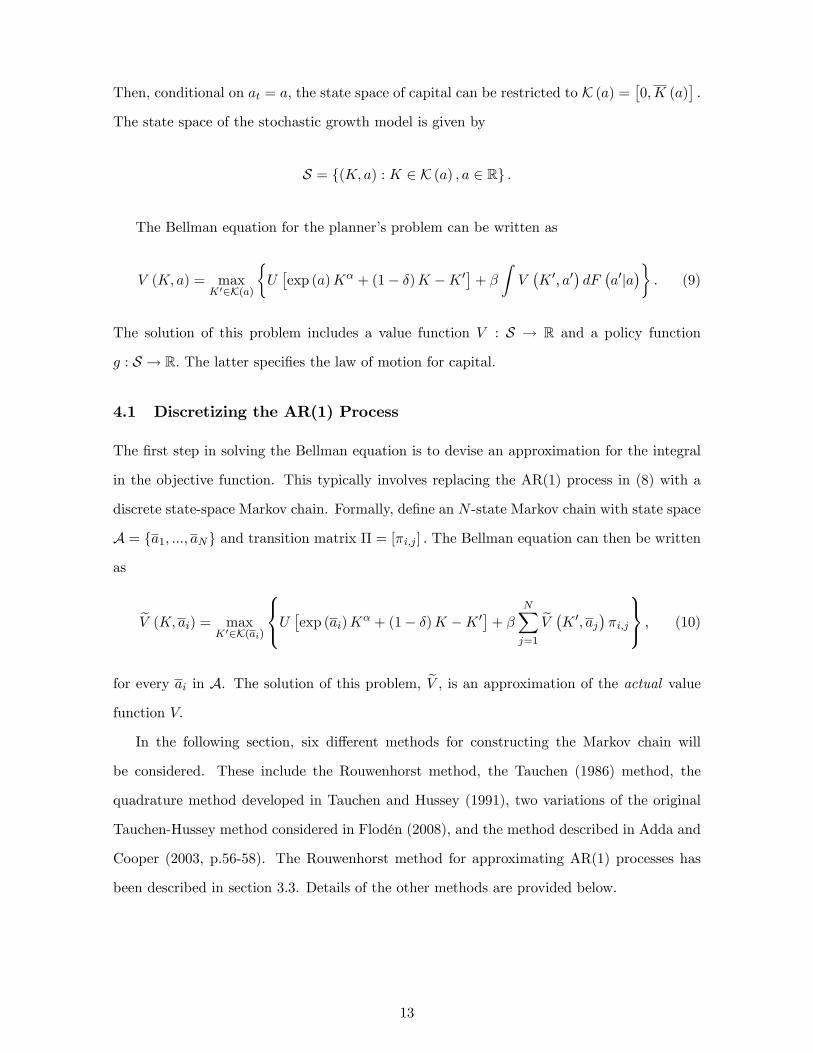
Then, conditional on at = a; the state space of capital can be restricted to K (a) =�0;K (a)

�:

The state space of the stochastic growth model is given by

S = f(K; a) : K 2 K (a) ; a 2 Rg :

The Bellman equation for the planner�s problem can be written as

V (K; a) = maxK02K(a)

�U�exp (a)K� + (1� �)K �K 0�+ � Z V

�K 0; a0

�dF�a0ja

��: (9)

The solution of this problem includes a value function V : S ! R and a policy function

g : S ! R: The latter speci�es the law of motion for capital.

4.1 Discretizing the AR(1) Process

The �rst step in solving the Bellman equation is to devise an approximation for the integral

in the objective function. This typically involves replacing the AR(1) process in (8) with a

discrete state-space Markov chain. Formally, de�ne an N -state Markov chain with state space

A = fa1; :::; aNg and transition matrix � = [�i;j ] : The Bellman equation can then be written

as

eV (K; ai) = maxK02K(ai)

8<:U �exp (ai)K� + (1� �)K �K 0�+ � NXj=1

eV �K 0; aj��i;j

9=; ; (10)

for every ai in A. The solution of this problem, eV ; is an approximation of the actual valuefunction V:

In the following section, six di¤erent methods for constructing the Markov chain will

be considered. These include the Rouwenhorst method, the Tauchen (1986) method, the

quadrature method developed in Tauchen and Hussey (1991), two variations of the original

Tauchen-Hussey method considered in Flodén (2008), and the method described in Adda and

Cooper (2003, p.56-58). The Rouwenhorst method for approximating AR(1) processes has

been described in section 3.3. Details of the other methods are provided below.

13

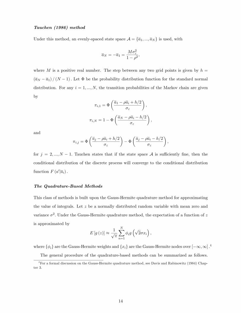
Tauchen (1986) method

Under this method, an evenly-spaced state space A = fa1; :::; aNg is used, with

aN = �a1 =M�2"1� �2 ;

where M is a positive real number. The step between any two grid points is given by h =

(aN � a1) = (N � 1) : Let � be the probability distribution function for the standard normal

distribution. For any i = 1; :::; N; the transition probabilities of the Markov chain are given

by

�i;1 = �

�a1 � �ai + h=2

�"

�;

�i;N = 1� ��aN � �ai � h=2

�"

�;

and

�i;j = �

�aj � �ai + h=2

�"

�� �

�aj � �ai � h=2

�"

�;

for j = 2; :::; N � 1: Tauchen states that if the state space A is su¢ ciently �ne, then the

conditional distribution of the discrete process will converge to the conditional distribution

function F (a0jai) :

The Quadrature-Based Methods

This class of methods is built upon the Gauss-Hermite quadrature method for approximating

the value of integrals. Let z be a normally distributed random variable with mean zero and

variance �2: Under the Gauss-Hermite quadrature method, the expectation of a function of z

is approximated by

E [g (z)] � 1p�

NXn=1

�ig�p2�xi

�;

where f�ig are the Gauss-Hermite weights and fxig are the Gauss-Hermite nodes over [�1;1] :4

The general procedure of the quadrature-based methods can be summarized as follows.

4For a formal discussion on the Gauss-Hermite quadrature method, see Davis and Rabinowitz (1984) Chap-ter 3.

14

First, the elements of the state space A are determined by

ai =p2�xi; for i = 1; 2; :::; N:

Second, the elements in the transition matrix � are given by

�i;j =f (aj jai)f (aj j0)

wjsi;

where wj = �j=p�; the function f (aj jai) is the density function for a normal distribution

with mean �ai and variance �2; and

si =NXn=1

f (anjai)f (anj0)

wn:

The only di¤erence between the original method considered in Tauchen and Hussey (1991)

and the variations considered in Flodén (2008) is the choice of �: In the original version,

the standard deviation � is taken to be �": In other words, the transition probabilities of

the Markov chain are constructed using the conditional density function of a: In the �rst

variation, the standard deviation of at is used instead, i.e., � = �a = �"=p1� �2. In the

second variation, � is a weighted average between �a and �": In particular,

� = !�" + (1� !)�a;

with ! = 0:5 + 0:25�:

The Adda-Cooper Method

The �rst step of this method is to partition the real line into N intervals. These intervals

are constructed so that the random variable at has an equal probability of falling into them.

Formally, let In = [xn; xn+1] be the nth interval with x1 = �1 and xN+1 = +1: The cut-o¤

points fxngNn=2 are obtained by solving the following system of equations:

�

�xn+1�a

�� �

�xn�a

�=1

N; for n = 1; 2; :::; N;

15

where � is the probability distribution function for the standard normal distribution. The

nth element in the state space A = fa1; :::; aNg is then given by the mean value of the nth

interval, i.e.,

an = E [aja 2 In] :

For any i; j 2 f1; 2; :::; Ng ; the transition probability �i;j is de�ned as the probability of

moving from interval Ii to interval Ij in one period. Formally, this is given by

�i;j = Pr�a0 2 Ij ja 2 Ii

�:

4.2 Experiments and Evaluation

The objective of this section is to evaluate the performance of di¤erent discretization methods.

To achieve this, we focus on the business cycle moments generated by the stochastic growth

model. The main criteria for evaluating the six discretization methods is the accuracy in

approximating these moments.

Solution Method

The �rst step in computing the business cycle moments is to choose a speci�c form for the

utility function and a set of values for the parameters f�; �; �; �"; �g : In the baseline model,

the utility function is logarithmic and there is full depreciation. The full depreciation assump-

tion is later relaxed in section 4.4. Under the baseline speci�cations, it is possible to derive

analytically (i) the policy functions for investment and consumption, (ii) the stationary dis-

tribution of the state variables, and (iii) the variances and �rst-order autocorrelations of the

endogenous variables. These closed-form solutions play a key role in evaluating the discretiza-

tion methods. This will become clear in subsequent discussions. The other parameter values

are chosen to be the same as in King and Rebelo (1999): � = 0:33; � = 0:984; �" = 0:0072

and � = 0:979:

The next step is to discretize the state space S of the stochastic growth model. First, the

AR(1) process in (8) is approximated using the methods mentioned above. The resulting N -

state Markov chain is characterized by a state space A = fa1; :::; aNg and a transition matrix

� = [�i;j ] : Second, the continuous state space for capital is replaced by an evenly-spaced grid.

16

De�ne the variable k � lnK: The set of grid points for k is represented by K =�k1; :::; kM

.

The discretized state space for the stochastic growth model can be expressed by

bS = ��km; an� : km 2 K; an 2 A : (11)

In the baseline case, the number of states in the Markov chain is set to �ve and the number

of grid points for capital is 1000. As reported in Flodén (2008), the performance of the

quadrature-based methods in approximating highly persistent processes is very sensitive to

the number of points in A. As a robustness check, we also consider the cases when N = 2 and

N = 10 in section 4.3. After the discrete state space bS is formed, the value function and theassociated policy function are solved using the value-function iteration method described in

Tauchen (1990) and Burnside (1999). The outcome of this procedure includes a set of N �M

values of the policy function evaluated on bS. This set of values is represented by �bg �km; an� :The �nal task is to compute the stationary distribution of the state variables (k; a) : The

�rst step to achieve this is to construct the transition matrix for these variables. Under the

discrete state-space method, the probability of moving from state�km; an

�in bS to another

state�kl; aj

�in bS in one period is speci�ed by

Pr��k0; a0

�=�kl; aj

�j (k; a) =

�km; an

��=

8><>: �n;j if kl = bg �km; an�0 otherwise.

(12)

The resulting NM -by-NM transition matrix is denoted P: Let b�=(b�1; :::; b�NM ) be the sta-tionary distribution associated with P: Formally, this is de�ned by

b�P = b�:In principle, b� can be obtained as the eigenvector of P corresponding to eigenvalue 1, with

the normalizationPNM

i=1 b�i = 1: This method, however, is not practical when the number ofgrid points for capital (M) or the number of grid points in the discrete Markov chain (N)

is large. In the following experiments, an approximation for the stationary distribution is

obtained by iterating the equation

e�lP = e�l+1: (13)

17

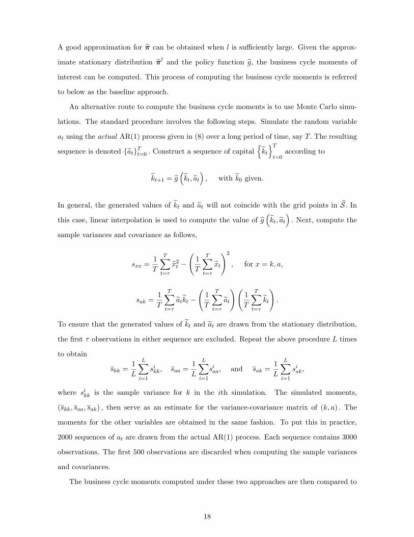
A good approximation for b� can be obtained when l is su¢ ciently large. Given the approx-imate stationary distribution e�l and the policy function bg; the business cycle moments ofinterest can be computed. This process of computing the business cycle moments is referred

to below as the baseline approach.

An alternative route to compute the business cycle moments is to use Monte Carlo simu-

lations. The standard procedure involves the following steps. Simulate the random variable

at using the actual AR(1) process given in (8) over a long period of time, say T: The resulting

sequence is denoted featgTt=0 : Construct a sequence of capital nektoTt=0

according to

ekt+1 = bg �ekt;eat� ; with ek0 given.In general, the generated values of ekt and eat will not coincide with the grid points in bS: Inthis case, linear interpolation is used to compute the value of bg �ekt;eat� : Next, compute thesample variances and covariance as follows,

sxx =1

T

TXt=�

ex2t � 1

T

TXt=�

ext!2 ; for x = k; a;

sak =1

T

TXt=�

eatekt � 1T

TXt=�

eat! 1T

TXt=�

ekt! :To ensure that the generated values of ekt and eat are drawn from the stationary distribution,

the �rst � observations in either sequence are excluded. Repeat the above procedure L times

to obtain

skk =1

L

LXi=1

sikk; saa =1

L

LXi=1

siaa; and sak =1

L

LXi=1

siak;

where sikk is the sample variance for k in the ith simulation. The simulated moments,

(skk; saa; sak) ; then serve as an estimate for the variance-covariance matrix of (k; a) : The

moments for the other variables are obtained in the same fashion. To put this in practice,

2000 sequences of at are drawn from the actual AR(1) process. Each sequence contains 3000

observations. The �rst 500 observations are discarded when computing the sample variances

and covariances.

The business cycle moments computed under these two approaches are then compared to

18

their true values obtained using the closed-form solutions. It turns out that the two approaches

would yield very di¤erent results. These di¤erences are reported in the error analysis section.

Baseline Results

Table 2 presents the baseline results obtained under the above procedure. The six discretiza-

tion methods are compared on three grounds: (i) the accuracy in approximating the AR(1)

process, (ii) the precision in approximating the stationary distribution of the state variables,

and (iii) the accuracy in approximating the business cycle moments. The true values obtained

under the closed-form solutions are used as the yardstick for comparison in each step.

Panel (A) of Table 2 shows the performance of these methods in approximating the AR(1)

process.5 As explained in section 3.3, the transition matrix in the Rouwenhorst method (R)

can be calibrated to match exactly the persistence parameter, the standard deviation of " and

the standard deviation of a: Among the other �ve methods, the Adda-Cooper method (A-C)

has the highest accuracy in terms of matching the persistence parameter. This is followed

by the second variation of the Tauchen-Hussey method (F-2), the Tauchen (1986) method

and the �rst variation of the Tauchen-Hussey method (F-1). The original Tauchen-Hussey

method has the lowest accuracy in terms of approximating the persistence parameter.

When it comes to matching the standard deviation of a, all �ve methods (excluding the

Rouwenhorst method) have di¢ culties in replicating the true value. With a relative error of

2.15 percent, the F-1 method has the best performance within this group. The other four

methods have relative errors ranging from �ve percent to 60 percent. In particular, the original

Tauchen-Hussey method can only replicate 40 percent of the actual value of �a: This problem

of the Tauchen-Hussey method is also reported in Flodén (2008). For the Tauchen (1986)

method, the F-2 method and the Adda-Cooper method, the low precision in approximating

�a is associated with a low precision in approximating �":

Next, we consider the accuracies of these methods in approximating the stationary dis-

tribution of the state variables. With a logarithmic utility function, full depreciation, and

"t following a Gaussian white noise process, the actual stationary distribution of (k; a) is a

5The relative errors reported in panel (A) are directly comparable to those reported in Flodén (2008) Table2 for n = 5 and � = 0:98: The only di¤erence is Flodén did not consider the Rouwenhorst method.

19

bivariate normal distribution with mean vector

�0 =

�ln(��)1�� 0

�;

and variance-covariance matrix

� =

264 �2k �ka

�ka �2a

375 ;where

�2k =(1 + ��)�2a

(1� �2) (1� ��) ;

�ka =��2a1� ��; and �2a =

�2"1� �2 :

Panel (B) of Table 2 shows the performance of these methods in approximating the stan-

dard deviation of k and the covariance between a and k. In general, a discretization method

that generates an accurate approximation for �a also has high precision in approximating

these two moments. Among these six methods, the Rouwenhorst method has the highest

accuracy in approximating these two moments. The relative errors for the two are about 0.14

percent. This outperforms the other methods by a signi�cant margin. The F-1 method, which

is the second best, has a relative error of about three percent in approximating �k and an

error of eight percent in approximating �ka:

Finally, we compare the performance of these methods in approximating the business

cycle moments. In particular, we focus on the standard deviation of output, consumption and

investment (in logarithmic terms) and the �rst-order autocorrelation of output (in logarithmic

terms).6 The results are shown in panel (C) of Table 2. Again the Rouwenhorst method has

the best performance in terms of approximating all these moments. The F-1 method is

the second best method in terms of �overall� performance. In terms of approximating the

�rst-order autocorrelation of output, the Tauchen (1986) method and the F-2 method are

actually more accurate than the F-1 method. However, the F-1 method performs better in

approximating the standard deviation of the endogenous variables.

6The �rst-order autocorrelation of consumption and investment (in logarithmic terms), and the cross-correlation between output and these variables are not shown in the paper. These results are available fromthe authors upon request.

20

Two things can be observed when comparing across all three panels. First, the relative

errors in approximating �a are very similar to those in approximating the standard deviation

of capital, output, consumption and investment. Second, the relative errors in approximating

� are close to those in approximating the �rst-order autocorrelation for output. These results

suggest that a good approximation for the moments of the AR(1) process is important in

obtaining an accurate approximation for the business cycle moments.

Error Analysis

The relative errors reported in Table 2 have a number of sources. For the purpose of this

discussion, we classify these into two groups. The �rst group of errors arises when solving the

Bellman equation in (9). This includes the errors that arise when we restrict the choice of

next-period capital to a discrete set of values, and the truncation errors that emerge when we

approximate the �xed point of the Bellman equation using a �nite number of iterations. The

second group of errors occurs during the computation of the stationary distribution of the state

variables. First, the transition matrix P , constructed using the discrete Markov chain and

the computed policy function, is an approximation of the actual transition function. Second,

truncation errors arise when we approximate the stationary distribution using a �nite number

of iterations. The second group of errors would not occur if Monte Carlo simulations are used

to generate the business cycle moments. In this case, however, a new source of error arises

when we estimate the actual moments by a �nite sample.

When the actual policy function is known, it is possible to disentangle the two groups

of errors. With logarithmic utility function and full depreciation, the policy function for

next-period capital (in logarithmic terms) is given by

kt+1 = g (kt; at) � ln�� + at + �kt: (14)

Now consider the following experiment. Construct a discrete state space bS as in (11) using oneof the six discretization methods. Construct the transition matrix P as in (12) but replace the

computed policy function bg (k; a) with the actual one in (14). Iterate equation (13) successivelyto obtain an approximation for the stationary distribution of the state variables. Finally, use

the approximate stationary distribution and the actual policy function g (k; a) to compute the

21

business cycle moments. By replacing bg (k; a) with the actual policy function, this proceduree¤ectively removes all the errors involved in solving the Bellman equation. The remaining

errors are thus due to the approximation of the stationary distribution of the state variables.

The results of this procedure are reported in panel (B) of Table 3. To facilitate comparison,

the baseline results are shown in panel (A) of the same table.

It is immediate to see that the �gures in the two panels are almost identical. Replacing

the computed policy function with the actual one does not a¤ect the approximation of the

technology shock process. As a result, the approximated values for �; �" and �a are identical

in the two sets of results. As for the standard deviations of the endogenous variables, only

minor discrepancies are observed in the two panels. In other words, even though we have

removed all the errors in computing the policy function, the baseline results remain largely

unchanged. This has two implications. First, this implies that almost all the relative errors in

the baseline case are due to the approximation of the stationary distribution b�: Second, thismeans the choice of discretization method has only a relatively minor impact on the solution

of the Bellman equation. In sum, this experiment illustrates that the choice of discretization

method matters because it would signi�cantly a¤ect the approximation of the stationary

distribution.

The same conclusion can be drawn from another experiment. Suppose now the business

cycle moments are computed using Monte Carlo simulations. More speci�cally, after solving

the dynamic programming problem in (9), the model is simulated using the actual AR(1)

process and the computed policy function bg (k; a) : Under this procedure, the choice of dis-cretization method only a¤ects the simulated moments through the computed policy function.

Table 4 presents the relative errors obtained under this procedure alongside with the baseline

results. The two methods of generating business cycle moments have produced very di¤erent

results. When the model is simulated using the actual AR(1) process, all six discretization

methods generate almost identical results. This again implies that the di¤erences in the

baseline results across the six discretization methods are due to the approximation of the

stationary distribution b�:The results in Table 4 also show that the accuracy of the Monte Carlo simulation method

cannot be taken for granted. This method is able to yield highly accurate estimates for �;

�" and �y: But it also yields a relative error of 2.6 percent when approximating the standard

22

deviations and an error of four percent when approximating �ka: When comparing between

these and the baseline results, it is obvious that the baseline approach, equipped with the

Rouwenhorst method, outperforms the Monte Carlo simulation method.

4.3 Robustness Check

In this section, it is shown that the relative performance of the six discretization methods are

robust to changes in (i) the number of points in the discrete state space N , (ii) the persistence

parameter �, and (iii) the standard deviation of the white noise process �":

Changing the Number of States

Table 5 compares the performance of the six methods under di¤erent choices of N . Intuitively,

increasing the number of states in the Markov chain should improve the performance of the

discretization methods. This is true for the Rouwenhorst method, the original Tauchen-Hussey

method, the F-2 method, and the Adda-Cooper method. However, this is not true for the

Tauchen (1986) method and the F-1 method.

The results in Table 5 show that the superior performance of the Rouwenhorst method

is robust even when there are only two states in the discrete Markov chain. As explained

in section 3.3, this method can always match the values of �; �" and �a regardless of the

choice of N: The relative errors in approximating the standard deviations of output, capital,

consumption and investment are similar in all three cases. In particular, increasing the number

of states from �ve to ten increases the precision only marginally. The original Tauchen-Hussey

method has the lowest precision among the six in all three cases. Even when the number of

states is increased to ten, the Tauchen-Hussey method can only replicate 57 percent of the

actual value of �y. The performance of this method is much better when approximating �y

but the precision is still the lowest among the six.

The performance of the F-2 method and the Adda-Cooper method improves signi�cantly

when the number of states increases. Similar to the baseline results, the F-2 method performs

better in terms of approximating the standard deviations of the endogenous variables, whereas

the Adda-Cooper method performs better in approximating �y:

Next, we consider the performance of the Tauchen (1986) method. As mentioned above,

the precision of this method does not necessarily improve when the number of states increases.

23

When there are only two states, the relative errors in approximating the standard deviations

are about sixteen percent. These drop to twelve percent when there are �ve states but rise

back to eighteen percent when there are ten states.7 In either case, the Tauchen (1986)

method has a lower precision than the Rouwenhorst method, the F-1 method and the Adda-

Cooper method. As in the baseline case, the Tauchen (1986) method performs better when

approximating �y: With a ten-state Markov chain, the relative error is about 0.16 percent,

which is among the lowest in the group. Finally, Table 5 shows that, in terms of approximating

the standard deviations, the F-1 method actually works best with a two-state Markov chain.

The relative error in approximating �y is a mere 0.65 percent when there are only two states.

Whereas, the relative error in approximating �y remains the same in all three cases.

Changing the Persistence Parameter

Table 6 compares the performance of the six methods under di¤erent values of �: The superior

performance of the Rouwenhorst method is robust to changes in this parameter. In particular,

increasing the persistence of the AR(1) process from 0.5 to 0.979 has very little impact on its

precision. This shows that the Rouwenhorst method is a reliable technique for approximating

stationary AR(1) process in general.

The performance of the three quadrature-based methods and the Tauchen (1986) method is

very sensitive to the value of �: Similar to Flodén (2008), our results show that the quadrature-

based method and the Tauchen (1986) method work best in approximating AR(1) processes

with low persistence. But unlike Flodén (2008) which only focuses on the parameters of the

AR(1) process, the current study also considers the impact of these methods on the mo-

ments of the endogenous variables. When � equals to 0.5 or 0.6, the original Tauchen-Hussey

method and its two variations can generate highly accurate approximations that are compara-

ble to those generated by the Rouwenhorst method. The relative errors for the business cycle

moments are all less than one percent. Within this range of �; the three quadrature-based

methods are more accurate than the Tauchen (1986) method. When � equals to 0.5, the

Tauchen (1986) method has a relative error of �ve percent in approximating �ka and an error

of two percent in approximating �y: However, the accuracies of the Tauchen-Hussey method

7A similar pattern is also observed in Flodén (2008) Table 2. The table shows that when � = 0:98; therelative error in approximating �a under the Tauchen (1986) method is 11.7 percent when N = 5 and 18.9percent when N = 10:

24

and the F-2 method deteriorate quickly when the persistence parameter approaches one. For

instance, the Tauchen-Hussey method has a relative error of 25 percent in approximating �y

when � equals to 0.9 and an error of 61 percent when � is 0.979. A similar but less dramatic

pattern is observed for the F-2 method. Among the three quadrature-based methods, the F-1

method is least sensitive to changes in the persistence parameter. Increasing this parameter

from 0.7 to 0.979 raises the relative errors in approximating �y from 0.39 percent to three

percent. The relative error in approximating �y increases from 0.88 percent to 1.1 percent

under the same change.

Unlike the quadrature-based methods, the Adda-Cooper method is more accurate when

the underlying AR(1) process is more persistent. When � equals to 0.5, the relative errors

in approximating �ka and �y are 20 percent and four percent, respectively. These reduce to

sixteen percent and two percent, respectively, when � is 0.979. The precision in approximating

the standard deviations does not seem to be a¤ected by the changes in �:

Finally, it is worth mentioning that the results of the two experiments conducted in the

error analysis section are also robust to di¤erent values of the persistence parameter. These

results are summarized as follow.8 First, the �gures reported in Table 6 are largely una¤ected

when we replace the computed policy function with the actual one. Second, when the business

cycle moments are computed using Monte Carlo simulations, all six discretization methods

generate very similar results.

Changing the Standard Deviation of the White Noise Process

The performance of the six methods under di¤erent values of �" are shown in Table 7. In

terms of approximating the AR(1) process, increasing the value of �" from 0.001 to 0.1 does

not seem to a¤ect the performance of these methods. In terms of approximating the standard

deviations of the endogenous variables and the covariance between a and k; the accuracies

of the Tauchen (1986) method, the original Tauchen-Hussey method, the F-2 method and

the Adda-Cooper method improve when the AR(1) process is less volatile. The opposite is

true for the Rouwenhorst method. The variations in the relative errors, however, are not

signi�cant. More speci�cally, increasing �" from 0.001 to 0.1 changes the relative errors by

less than two percentage points in most cases. Unlike the other methods, the performance of

8The numerical results are not shown in the paper but are available from the authors upon request.

25

the F-1 method is more sensitive to the value of �": For instance, when �" equals to 0.001

the relative errors in approximating �k and �ka are 0.5 percent and �ve percent, respectively.

These become 1.6 percent and 2.3 percent, respectively, when �" is 0.1. Finally, the precision

of all six methods in approximating �y is not sensitive to changes in the value of �":

4.4 Relaxing the Assumption of Full Depreciation

This section evaluates the performance of the six discretization methods in solving the stochas-

tic growth model when the full depreciation assumption is relaxed. The rate of depreciation

is now taken to be 2.5 percent, which is the same as in King and Rebelo (1999). All other

parameters remain the same as in the baseline case. The same evaluation process is performed

as in section 4.2. For each of the six discretization methods, we compute the business cycle

moments using the baseline approach and the Monte Carlo simulation method. Without full

depreciation, however, a closed-form solution for the policy function is not available and the

actual values of the business cycle moments are unknown. Thus we derive a highly accurate

approximation for the actual moments which is then used as our yardstick for comparison.

To achieve this, we �rst construct an extremely �ne discrete state space with 2000 grid points

for capital and 400 states in the Markov chain constructed by the Rouwenhorst method. We

then compute the business cycle moments using the baseline approach described earlier. The

rationale for this procedure is as follows. As explained in the error analysis section, the base-

line approach involves two groups of errors: (i) errors that arise when solving the Bellman

equation, and (ii) errors that arise when computing the stationary distribution. When the

number of grid points in the discrete state space is su¢ ciently large, the value function iter-

ation method is able to yield highly accurate solutions for the Bellman equation. Thus, by

adopting an extremely �ne state space, the above procedure should render the �rst group of

errors very small. As for the second group of errors, our baseline results for the full depre-

ciation case show that combining the Rouwenhorst method and the baseline approach can

yield a highly accurate approximation for the stationary distribution. As a robustness check

on this procedure, we double the size of the state space and �nd that it has no e¤ect on the

computed statistics. The business cycle moments obtained under this procedure are referred

to below as the true solutions.

The main �ndings of this exercise are as follows. First, the superior performance of the

26

baseline approach combined with the Rouwenhorst discretization method is robust to relaxing

the full depreciation assumption. Second, the overall performance of the other methods

deteriorates signi�cantly when � is less than one. Panel (A) of Table 8 shows the results

obtained under the baseline approach for three di¤erent values of N . Panel (B) of the same

table reports the simulation results. First note that the Rouwenhorst method has the best

overall performance for each grid sizeN when comparing both across columns in Panel (A) and

between Panels (A) and (B). Thus the Rouwenhorst method under the baseline approach is

not only superior to the other methods but also to computing the statistics using Monte Carlo

simulations. Second, note that the overall performance of the other methods, as measured

by the size of the relative errors in their estimates, is substantially worse with � set at 2.5

percent than in the full depreciation case (Tables 2 and 5). This is particularly true for the

estimates of �ka and �i. For example, consider the F-1 method which has the second highest

precision in the full depreciation case. With only �ve states in the Markov chain and full

depreciation, this method generates a relative error of eight percent in approximating �ka and

an error of about three percent in approximating �i (see Table 2). These become 26 percent

and 21 percent, respectively, when � equals 0.025. In contrast, relaxing the full depreciation

assumption has only a negligible e¤ect on the estimates of �y.

A closer look at Panel (A) of Table 8 reveals that, similar to the results in Table 5,

increasing the number of states in the Markov chain usually improves the accuracy of the

approximations. However, the performance of the methods varies signi�cantly when it comes

to approximating the standard deviations and the covariance between k and a, even when

N is large. For the Rouwenhorst method, a �ve-fold increase in the number of states only

marginally a¤ects the precision of the results. However, unlike the full depreciation case,

increasing the number of states does not always improve the precision. In particular, the

relatively large error in approximating �i remains even when there are 25 states. For the

original Tauchen-Hussey method, its performance improves signi�cantly when the �neness

of the state space increases. However, even when there are 25 states, this method can only

replicate 67 percent of the true value of �ka and 83 percent of the true value of �y. The overall

performance of the Tauchen (1986) method and the F-1 method is also rather disappointing

in this case. A �ve-fold increase in the number of states does not seem to have a signi�cant

impact on their precision. On the other hand, when N is large the F-2 method is able to yield

27

highly accurate approximations that are comparable to those generated by the Rouwenhorst

method. It thus has the best performance among the three quadrature-based methods. As

for the Adda-Cooper method, relatively large errors remain even when there are 25 states.

For instance, the relative errors in approximating �ka and �i are about �ve percent.

Unlike the full depreciation case, the six discretization methods under the Monte Carlo

simulation approach do not generate near identical results. This can be seen by comparing

the columns in Panel (B) of Table 8. Thus the choice of discretization method matters even

when the business cycle moments are computed using Monte Carlo simulations. This is due

to the following reason. In the absence of full depreciation, the policy function for next-period

capital (in logarithms), represented by

kt+1 = g(kt; at);

is no longer a linear function. Consequently, additional approximation errors arise when

we compute g(kt; at) for values of kt and at that are outside the discrete state space. The

size of these errors depends on the location of the grid points and hence the choice of the

discretization method. As the number of states in the Markov chain increases, the state space

becomes �ner and the errors associated with the interpolation procedure falls. For this reason,

a �ve-fold increase in N signi�cantly reduces the relative errors of the discretization methods.

Finally, under the Monte Carlo simulation approach, no single method dominates all others

in all three choices of N . When there are �ve states in the Markov chain, the Rouwenhorst

method has the best overall performance within the group. But when there are 25 states,

the Adda-Cooper method has the best overall performance. In this case, the Tauchen (1986)

method, the original Tauchen-Hussey method and the F-2 method all perform equally well as

the Rouwenhorst method.

5 Conclusions

This paper re-examines the Rouwenhorst method of constructing a discrete-valued Markov

chain to approximate a given �rst-order autoregressive process. Under this method, the con-

structed Markov chain can be calibrated to match the conditional and unconditional mean,

the conditional and unconditional variance and the �rst-order autocorrelation of any station-

28

ary AR(1) process. Because of this distinctive feature, the Rouwenhorst method is more

reliable than the Tauchen (1986) method and the Tauchen-Hussey method to approximate

highly persistent processes. In this paper, a new and simpler procedure for generating the

transition matrix in the Rouwenhorst method is developed and the �rst formal proof for all

the important properties of the constructed Markov chain is provided.

In the quantitative analysis, the Rouwenhorst method is compared to �ve other discretiza-

tion methods. These methods are evaluated based on their performance in approximating the

business cycle moments generated by the standard neoclassical growth model without leisure.

Two approaches to generate these moments are considered. In the baseline approach, an

approximation for the stationary distribution of the state variables is �rst computed. In the

second approach, the moments of interest are generated using Monte Carlo simulations. Our

quantitative analysis yields two important messages. First, under both approaches, the choice

of approximation method can have a large impact on the accuracy of the solutions. Under the

baseline approach, an accurate approximation of the moments of the AR(1) process is im-

portant in accurately approximating the business cycle moments. The Rouwenhorst method

has the best performance in this regard and outperforms the other methods by a signi�cant

margin. Its superior performance is robust under a wide range of parameter values. Under the

second approach, no single method dominates all others in all cases. When a realistic value of

the depreciation rate is used, the Rouwenhorst method again has the best overall performance

when there are only �ve states in the Markov chain. However, when the �neness of the state

space increases, the Adda-Cooper method improves signi�cantly and yields the best overall

performance. Second, the simulation method is not the best approach to generate the business

cycle statistics in the neoclassical growth model. Our results show that the combination of

the baseline approach and the Rouwenhorst method has a higher degree of accuracy than the

simulation method.

In this paper, we use a standard representative-agent model as our test model. We believe

that similar results can be obtained in heterogeneous-agent economies. However, we leave a

detailed exploration of these models for future research.

29

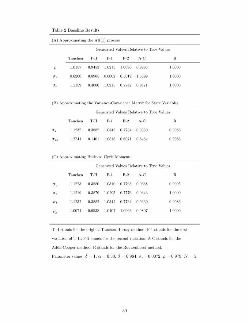
Table 2 Baseline Results

(A) Approximating the AR(1) process

Generated Values Relative to True Values

Tauchen T-H F-1 F-2 A-C R

� 1.0157 0.9453 1.0215 1.0096 0.9993 1.0000

�" 0.6260 0.8905 0.0002 0.5019 1.5599 1.0000

�a 1.1159 0.4006 1.0215 0.7742 0.9471 1.0000

(B) Approximating the Variance-Covariance Matrix for State Variables

Generated Values Relative to True Values

Tauchen T-H F-1 F-2 A-C R

�k 1.1232 0.3882 1.0342 0.7734 0.9330 0.9986

�ka 1.2741 0.1401 1.0818 0.6071 0.8464 0.9986

(C) Approximating Business Cycle Moments

Generated Values Relative to True Values

Tauchen T-H F-1 F-2 A-C R

�y 1.1223 0.3880 1.0310 0.7763 0.9338 0.9995

�c 1.1219 0.3879 1.0295 0.7776 0.9343 1.0000

�i 1.1232 0.3882 1.0342 0.7734 0.9330 0.9986

�y 1.0074 0.9538 1.0107 1.0063 0.9807 1.0000

T-H stands for the original Tauchen-Hussey method; F-1 stands for the �rst

variation of T-H; F-2 stands for the second variation; A-C stands for the

Adda-Cooper method; R stands for the Rouwenhorst method.

Parameter values: � = 1; � = 0:33; � = 0:984; �"= 0:0072; � = 0:979; N = 5:

30

Table 3 Error Analysis

(A) Using Computed Policy Function (Baseline case)

Generated Values Relative to True Values

Tauchen T-H F-1 F-2 A-C R

� 1.0157 0.9453 1.0215 1.0096 0.9993 1.0000

�" 0.6260 0.8905 0.0002 0.5019 1.5599 1.0000

�a 1.1159 0.4006 1.0215 0.7742 0.9471 1.0000

�k 1.1232 0.3882 1.0342 0.7734 0.9330 0.9986

�ka 1.2741 0.1401 1.0818 0.6071 0.8464 0.9986

�y 1.1223 0.3880 1.0310 0.7763 0.9338 0.9995

�c 1.1219 0.3879 1.0295 0.7776 0.9343 1.0000

�i 1.1232 0.3882 1.0342 0.7734 0.9330 0.9986

�y 1.0074 0.9538 1.0107 1.0063 0.9807 1.0000

(B) Using Actual Policy Function

Generated Values Relative to True Values

Tauchen T-H F-1 F-2 A-C R

� 1.0157 0.9453 1.0215 1.0096 0.9993 1.0000

�" 0.6260 0.8905 0.0002 0.5019 1.5599 1.0000

�a 1.1159 0.4006 1.0212 0.7742 0.9471 1.0000

�k 1.1219 0.3880 1.0292 0.7777 0.9343 1.0000

�ka 1.2726 0.1400 1.0762 0.6104 0.8475 1.0000

�y 1.1219 0.3879 1.0292 0.7777 0.9343 1.0000

�c 1.1219 0.3879 1.0292 0.7777 0.9343 1.0000

�i 1.1219 0.3880 1.0292 0.7777 0.9343 1.0000

�y 1.0074 0.9537 1.0107 1.0063 0.9807 1.0000

T-H stands for the original Tauchen-Hussey method; F-1 stands for the

�rst variation of T-H; F-2 stands for the second variation; A-C stands for

the Adda-Cooper method; R stands for the Rouwenhorst method.

Parameter values: � = 1; � = 0:33; � = 0:984; �"= 0:0072; � = 0:979; N = 5:

31

Table 4 Baseline Approach vs. Monte Carlo Simulations

(A) Baseline case

Generated Values Relative to True Values

Tauchen T-H F-1 F-2 A-C R

� 1.0157 0.9453 1.0215 1.0096 0.9993 1.0000

�" 0.6260 0.8905 0.0002 0.5019 1.5599 1.0000

�a 1.1159 0.4006 1.0215 0.7742 0.9471 1.0000

�k 1.1232 0.3882 1.0342 0.7734 0.9330 0.9986

�ka 1.2741 0.1401 1.0818 0.6071 0.8464 0.9986

�y 1.1223 0.3880 1.0310 0.7763 0.9338 0.9995

�c 1.1219 0.3879 1.0295 0.7776 0.9343 1.0000

�i 1.1232 0.3882 1.0342 0.7734 0.9330 0.9986

�y 1.0074 0.9538 1.0107 1.0063 0.9807 1.0000

(B) Monte Carlo Simulations

Generated Values Relative to True Values

Tauchen T-H F-1 F-2 A-C R

� 0.9983 0.9983 0.9983 0.9983 0.9983 0.9983

�" 1.0001 1.0001 1.0001 1.0001 1.0001 1.0001

�a 0.9748 0.9748 0.9748 0.9748 0.9748 0.9748

�k 0.9744 0.9745 0.9745 0.9745 0.9746 0.9745

�ka 0.9575 0.9575 0.9575 0.9575 0.9576 0.9575

�y 0.9744 0.9744 0.9744 0.9744 0.9744 0.9744

�c 0.9744 0.9744 0.9744 0.9744 0.9744 0.9744

�i 0.9744 0.9745 0.9745 0.9745 0.9746 0.9745

�y 0.9991 0.9991 0.9991 0.9991 0.9991 0.9991

T-H stands for the original Tauchen-Hussey method; F-1 stands for the

�rst variation of T-H; F-2 stands for the second variation; A-C stands for

the Adda-Cooper method; R stands for the Rouwenhorst method.

Parameter values: � = 1; � = 0:33; � = 0:984; �"= 0:0072; � = 0:979; N = 5:

32

Table5ChangingtheNumberofStatesintheMarkovChain

N=2

N=5(Baseline)

N=10

GeneratedValuesRelativetoTrueValues

GeneratedValuesRelativetoTrueValues

GeneratedValuesRelativetoTrueValues

Tau

T-H

F-1

F-2

A-C

RTau

T-H

F-1

F-2

A-C

RTau

T-H

F-1

F-2

A-C

R

�1.0214

0.7688

1.0215

1.0206

0.8879

1.0000

1.0157

0.9453

1.0215

1.0096

0.9993

1.0000

1.0045

0.9867

1.0214

1.0006

1.0038

1.0000

�"

0.0465

0.6584

0.0000

0.0805

1.9346

1.0000

0.6260

0.8905

0.0002

0.5019

1.5599

1.0000

1.0963

0.9493

0.0225

0.8886

1.2781

1.0000

�a

0.8318

0.2039

1.0000

0.4071

0.7979

1.0000

1.1159

0.4006

1.0215

0.7742

0.9471

1.0000

1.1874

0.5860

1.0076

0.9558

0.9793

1.0000

�k

0.8433

0.1844

1.0040

0.4095

0.7718

0.9966

1.1232

0.3882

1.0342

0.7734

0.9330

0.9986

1.1892

0.5794

1.0122

0.9583

0.9753

0.9988

�ka

0.7183

0.0283

1.0281

0.1705

0.5400

0.9966

1.2741

0.1401

1.0818

0.6071

0.8464

0.9986

1.4171

0.3260

1.0444

0.9190

0.9386

0.9988

�y

0.8399

0.1870

1.0065

0.4099

0.7682

0.9989

1.1223

0.3880

1.0310

0.7763

0.9338

0.9995

1.1889

0.5788

1.0144

0.9573

0.9743

0.9996

�c

0.8383

0.1882

1.0078

0.4101

0.7664

1.0000

1.1219

0.3879

1.0295

0.7776

0.9343

1.0000

1.1888

0.5784

1.0154

0.9569

0.9739

1.0000

�i

0.8433

0.1844

1.0040

0.4095

0.7718

0.9966

1.1232

0.3882

1.0342

0.7734

0.9330

0.9986

1.1892

0.5794

1.0122

0.9583

0.9753

0.9988

�y

1.0107

0.8752

1.0107

1.0103

0.9422

1.0000

1.0074

0.9538

1.0107

1.0063

0.9807

1.0000

1.0016

0.9817

1.0107

1.0015

0.9922

1.0000

TaustandsfortheTauchen(1986)method;T-HstandsfortheoriginalTauchen-Husseymethod;F-1standsforthe�rstvariationofT-H;F-2standsforthe

secondvariation;A-CstandsfortheAdda-Coopermethod;RstandsfortheRouwenhorstmethod.

Parametervalues:�=1;�=0:33;�=0:984;�"=0:0072;�=0:979:

33

Table6ChangingthePersistenceParameter

�=0:5

�=0:6

�=0:7

GeneratedValuesRelativetoTrueValues

GeneratedValuesRelativetoTrueValues

GeneratedValuesRelativetoTrueValues

Tau

T-H

F-1

F-2

A-C

RTau

T-H

F-1

F-2

A-C

RTau

T-H

F-1

F-2

A-C

R

�0.9686

0.9997

1.0007

1.0000

0.9310

1.0000

0.9739

0.9986

1.0039

0.9999

0.9471

1.0000

0.9798

0.9953

1.0174

0.9997

0.9665

1.0000

�"

1.0139

0.9994

0.9998

0.9999

0.9737

1.0000

1.0234

0.9972

0.9977

0.9993

0.9888

1.0000

1.0392

0.9905

0.9819

0.9969

1.0112

1.0000

�a

1.0012

0.9990

0.9999

0.9999

0.9471

1.0000

1.0035

0.9950

0.9996

0.9993

0.9471

1.0000

1.0085

0.9793

0.9982

0.9963

0.9471

1.0000

�k

0.9973

1.0025

0.9973

1.0048

0.9364

1.0010

0.9983

0.9973

0.9988

1.0017

0.9345

0.9991

0.9996

0.9788

1.0085

0.9969

0.9243

0.9983

�ka

0.9581

0.9995

0.9971

1.0035

0.8050

1.0011

0.9629

0.9873

1.0021

0.9998

0.8072

0.9981

0.9734

0.9456

1.0238

0.9925

0.8050

0.9985

�y

0.9952

0.9996

0.9993

1.0009

0.9336

1.0002

0.9964

0.9948

1.0000

0.9997

0.9316

0.9996

1.0003

0.9769

1.0039

0.9963

0.9282

0.9996

�c

0.9944

0.9983

1.0004

0.9992

0.9324

1.0001

0.9957

0.9938

1.0006

0.9989

0.9304

1.0000

1.0007

0.9761

1.0018

0.9962

0.9302

1.0003

�i

0.9973

1.0025

0.9973

1.0048

0.9364

1.0010

0.9983

0.9973

0.9988

1.0017

0.9345

0.9991

0.9996

0.9788

1.0085

0.9969

0.9243

0.9983

�y

0.9824

1.0002

0.9997

1.0009

0.9588

1.0001

0.9828

0.9985

1.0014

1.0003

0.9599

0.9999

0.9836

0.9943

1.0088

0.9997

0.9613

0.9998

TaustandsfortheTauchen(1986)method;T-HstandsfortheoriginalTauchen-Husseymethod;F-1standsforthe�rstvariationofT-H;F-2standsforthe

secondvariation;A-CstandsfortheAdda-Coopermethod;RstandsfortheRouwenhorstmethod.

Parametervalues:�=1;�=0:33;�=0:984;�"=0:0072;N=5:

34

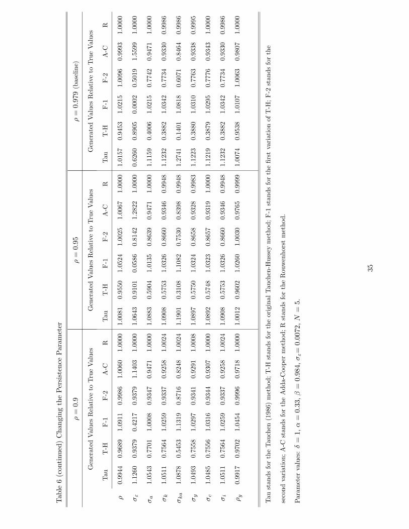
Table6(continued)ChangingthePersistenceParameter

�=0:9

�=0:95

�=0:979(baseline)

GeneratedValuesRelativetoTrueValues

GeneratedValuesRelativetoTrueValues

GeneratedValuesRelativetoTrueValues

Tau

T-H

F-1

F-2

A-C

RTau

T-H

F-1

F-2

A-C

RTau

T-H

F-1

F-2

A-C

R

�0.9944

0.9689

1.0911

0.9986

1.0060

1.0000

1.0081

0.9550

1.0524

1.0025

1.0067

1.0000

1.0157

0.9453

1.0215

1.0096

0.9993

1.0000

�"

1.1260

0.9379

0.4217

0.9379

1.1403

1.0000

1.0643

0.9101

0.0586

0.8142

1.2822

1.0000

0.6260

0.8905

0.0002

0.5019

1.5599

1.0000

�a

1.0543

0.7701

1.0008

0.9347

0.9471

1.0000

1.0883

0.5904

1.0135

0.8639

0.9471

1.0000

1.1159

0.4006

1.0215

0.7742

0.9471

1.0000

�k

1.0511

0.7564

1.0259

0.9337

0.9258

1.0024

1.0908

0.5753

1.0326

0.8660

0.9346

0.9948

1.1232

0.3882

1.0342

0.7734

0.9330

0.9986

�ka

1.0878

0.5453

1.1319

0.8716

0.8248

1.0024

1.1901

0.3108

1.1082

0.7530

0.8398

0.9948

1.2741

0.1401

1.0818

0.6071

0.8464

0.9986

�y

1.0493

0.7558

1.0297

0.9341

0.9291

1.0008

1.0897

0.5750

1.0324

0.8658

0.9328

0.9983

1.1223

0.3880

1.0310

0.7763

0.9338

0.9995

�c

1.0485

0.7556

1.0316

0.9344

0.9307

1.0000

1.0892

0.5748

1.0323

0.8657

0.9319

1.0000

1.1219

0.3879

1.0295

0.7776

0.9343

1.0000

�i

1.0511

0.7564

1.0259

0.9337

0.9258

1.0024

1.0908

0.5753

1.0326

0.8660

0.9346

0.9948

1.1232

0.3882

1.0342

0.7734

0.9330

0.9986

�y

0.9917

0.9702

1.0454

0.9996

0.9718

1.0000

1.0012

0.9602

1.0260

1.0030

0.9765

0.9999

1.0074

0.9538

1.0107

1.0063

0.9807

1.0000

TaustandsfortheTauchen(1986)method;T-HstandsfortheoriginalTauchen-Husseymethod;F-1standsforthe�rstvariationofT-H;F-2standsforthe

secondvariation;A-CstandsfortheAdda-Coopermethod;RstandsfortheRouwenhorstmethod.

Parametervalues:�=1;�=0:33;�=0:984;�"=0:0072;N=5:

35

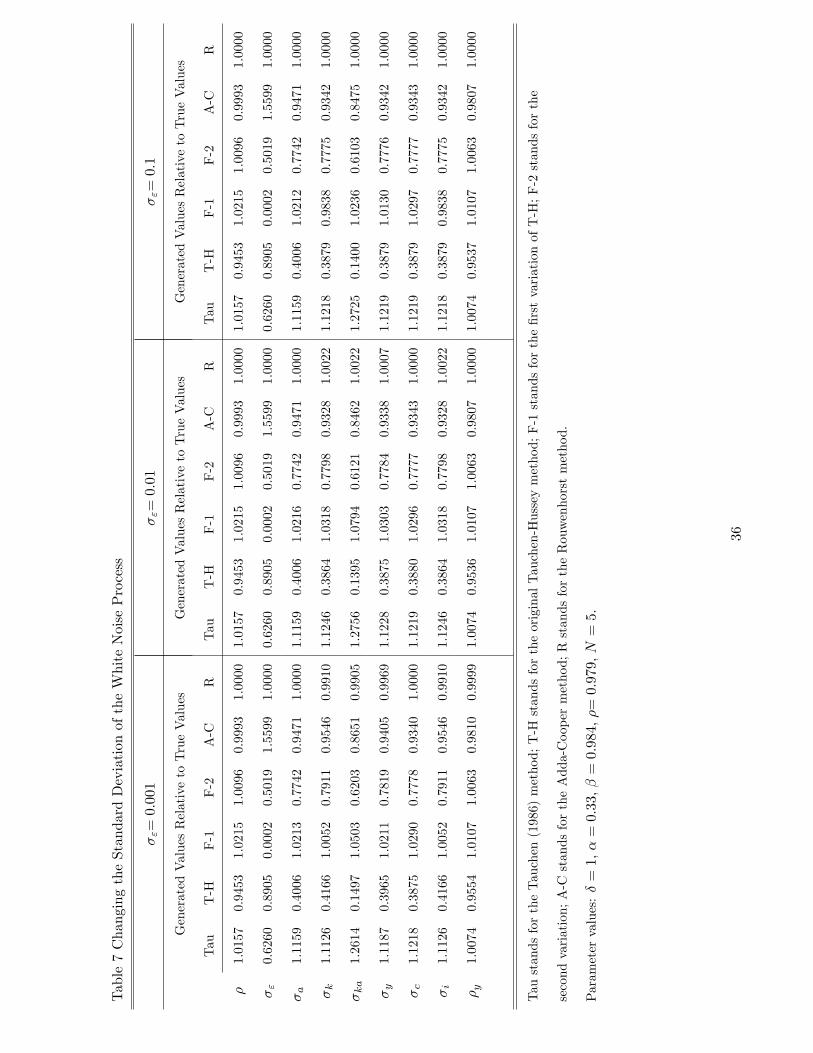
Table7ChangingtheStandardDeviationoftheWhiteNoiseProcess

�"=0:001

�"=0:01

�"=0:1

GeneratedValuesRelativetoTrueValues

GeneratedValuesRelativetoTrueValues

GeneratedValuesRelativetoTrueValues

Tau

T-H

F-1

F-2

A-C

RTau

T-H

F-1

F-2

A-C

RTau

T-H

F-1

F-2

A-C

R

�1.0157

0.9453

1.0215

1.0096

0.9993

1.0000

1.0157

0.9453

1.0215

1.0096

0.9993

1.0000

1.0157

0.9453

1.0215

1.0096

0.9993

1.0000

�"

0.6260

0.8905

0.0002

0.5019

1.5599

1.0000

0.6260

0.8905

0.0002

0.5019

1.5599

1.0000

0.6260

0.8905

0.0002

0.5019

1.5599

1.0000

�a

1.1159

0.4006

1.0213

0.7742

0.9471

1.0000

1.1159

0.4006

1.0216

0.7742

0.9471

1.0000

1.1159

0.4006

1.0212

0.7742

0.9471

1.0000

�k

1.1126

0.4166

1.0052

0.7911

0.9546

0.9910

1.1246

0.3864

1.0318

0.7798

0.9328

1.0022

1.1218

0.3879

0.9838

0.7775

0.9342

1.0000

�ka

1.2614

0.1497

1.0503

0.6203

0.8651

0.9905

1.2756

0.1395

1.0794

0.6121

0.8462

1.0022

1.2725

0.1400

1.0236

0.6103

0.8475

1.0000

�y

1.1187

0.3965

1.0211

0.7819

0.9405

0.9969

1.1228

0.3875

1.0303

0.7784

0.9338

1.0007

1.1219

0.3879

1.0130

0.7776

0.9342

1.0000

�c

1.1218

0.3875

1.0290

0.7778

0.9340

1.0000

1.1219

0.3880

1.0296

0.7777

0.9343

1.0000

1.1219

0.3879

1.0297

0.7777

0.9343

1.0000

�i

1.1126

0.4166

1.0052

0.7911

0.9546

0.9910

1.1246

0.3864

1.0318

0.7798

0.9328

1.0022

1.1218

0.3879

0.9838

0.7775

0.9342

1.0000

�y

1.0074

0.9554

1.0107

1.0063

0.9810

0.9999

1.0074

0.9536

1.0107

1.0063

0.9807

1.0000

1.0074

0.9537

1.0107

1.0063

0.9807

1.0000

TaustandsfortheTauchen(1986)method;T-HstandsfortheoriginalTauchen-Husseymethod;F-1standsforthe�rstvariationofT-H;F-2standsforthe

secondvariation;A-CstandsfortheAdda-Coopermethod;RstandsfortheRouwenhorstmethod.

Parametervalues:�=1;�=0:33;�=0:984;�=0:979;N=5:

36

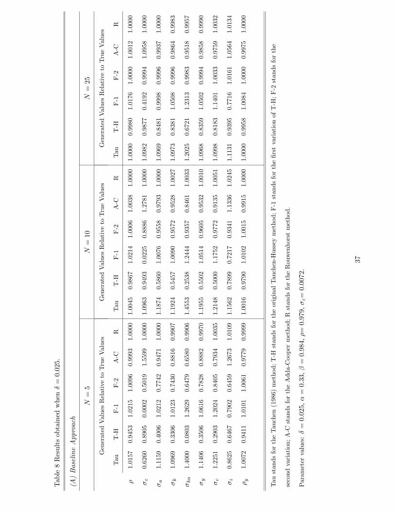
Table8Resultsobtainedwhen�=0:025:

(A)BaselineApproach

N=5

N=10

N=25

GeneratedValuesRelativetoTrueValues

GeneratedValuesRelativetoTrueValues

GeneratedValuesRelativetoTrueValues

Tau

T-H

F-1

F-2

A-C

RTau

T-H

F-1

F-2

A-C

RTau

T-H

F-1

F-2

A-C

R

�1.0157

0.9453

1.0215

1.0096

0.9993

1.0000

1.0045

0.9867

1.0214

1.0006

1.0038

1.0000

1.0000

0.9980

1.0176

1.0000

1.0012

1.0000

�"

0.6260

0.8905

0.0002

0.5019

1.5599

1.0000

1.0963

0.9493

0.0225

0.8886

1.2781

1.0000

1.0982

0.9877

0.4192

0.9994

1.0958

1.0000

�a

1.1159

0.4006

1.0212

0.7742

0.9471

1.0000

1.1874

0.5860

1.0076

0.9558

0.9793

1.0000

1.0969

0.8481

0.9998

0.9996

0.9937

1.0000

�k

1.0969

0.3306

1.0123

0.7430

0.8816

0.9907

1.1924

0.5457

1.0090

0.9572

0.9528

1.0027

1.0973

0.8381

1.0508

0.9996

0.9864

0.9983

�ka

1.4000

0.0803

1.2629

0.6479

0.6580

0.9906

1.4553

0.2538

1.2444

0.9357

0.8461

1.0033

1.2025

0.6721

1.2313

0.9983

0.9518

0.9957

�y

1.1406

0.3506

1.0616

0.7828

0.8882

0.9970

1.1955

0.5502

1.0514

0.9605

0.9532

1.0010

1.0968

0.8359

1.0502

0.9994

0.9858

0.9990

�c

1.2251

0.2903

1.2024

0.8405

0.7934

1.0035

1.2148

0.5000

1.1752

0.9772

0.9135

1.0051

1.0998

0.8183

1.1401

1.0033

0.9759

1.0032

�i

0.8625

0.6467

0.7902

0.6459

1.2673

1.0109

1.1562

0.7899

0.7217

0.9341

1.1336

1.0245

1.1131

0.9395

0.7716

1.0161

1.0564

1.0134

�y

1.0072

0.9411

1.0101

1.0061

0.9779

0.9999

1.0016

0.9790

1.0102

1.0015

0.9915

1.0000

1.0000

0.9958

1.0084

1.0000

0.9975

1.0000

TaustandsfortheTauchen(1986)method;T-HstandsfortheoriginalTauchen-Husseymethod;F-1standsforthe�rstvariationofT-H;F-2standsforthe

secondvariation;A-CstandsfortheAdda-Coopermethod;RstandsfortheRouwenhorstmethod.

Parametervalues:�=0:025;�=0:33;�=0:984;�=0:979;�"=0:0072:

37

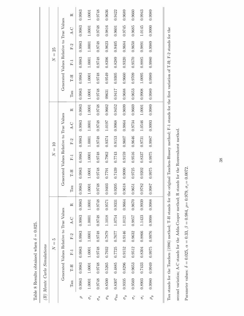
Table8Resultsobtainedwhen�=0:025:

(B)MonteCarloSimulations N=5

N=10

N=25

GeneratedValuesRelativetoTrueValues

GeneratedValuesRelativetoTrueValues

GeneratedValuesRelativetoTrueValues

Tau

T-H

F-1

F-2

A-C

RTau

T-H

F-1

F-2

A-C

RTau

T-H

F-1

F-2

A-C

R

�0.9983

0.9983

0.9983

0.9983

0.9983

0.9983

0.9983

0.9983

0.9983

0.9983

0.9983

0.9983

0.9983

0.9983

0.9983

0.9983

0.9983

0.9983

�"

1.0001

1.0001

1.0001

1.0001

1.0001

1.0001

1.0001

1.0001

1.0001

1.0001

1.0001

1.0001

1.0001

1.0001

1.0001

1.0001

1.0001

1.0001

�a

0.9748

0.9748

0.9748

0.9748

0.9748

0.9748

0.9748

0.9748

0.9748

0.9748

0.9748

0.9748

0.9748

0.9748

0.9748

0.9748

0.9748

0.9748

�k

0.8500

0.5265

0.7932

0.7879

1.1018

0.9571

0.9403

0.7791

0.7962

0.9374

1.0197

0.9662

09631

0.9549

0.8396

0.9623

0.9816

0.9636

�ka

0.8307

0.4885

0.7725

0.7677

1.0754

0.9331

0.9205

0.7439

0.7743

0.9153

0.9968

0.9452

0.9417

0.9305

0.8289

0.9405

0.9601

0.9422

�y

0.9335

0.8296

0.9152

0.9146

1.0121

0.9664

0.9618

0.9090

0.9159

0.9607

0.9864

0.9699

0.9688

0.9660

0.9320

0.9684

0.9745

0.9689

�c

0.9569

0.9653

0.9512

0.9632

0.9857

0.9670

0.9651

0.9725

0.9516

0.9646

0.9734

0.9669

0.9653

0.9709

0.9570

0.9650

0.9685

0.9660

�i

0.8903

0.7433

0.8304

0.8866

1.1423

0.9939

0.9782

0.9202

0.8337

0.9731

1.0546

1.0001

0.9908

1.0095

0.8885

0.9891

1.0145

0.9943

�y

0.9980

0.9949

0.9975

0.9976

0.9998

0.9988

0.9987

0.9975

0.9975

0.9987

0.9993

0.9989

0.9989

0.9989

0.9980

0.9989

0.9990

0.9989

TaustandsfortheTauchen(1986)method;T-HstandsfortheoriginalTauchen-Husseymethod;F-1standsforthe�rstvariationofT-H;F-2standsforthe

secondvariation;A-CstandsfortheAdda-Coopermethod;RstandsfortheRouwenhorstmethod.

Parametervalues:�=0:025;�=0:33;�=0:984;�=0:979;�"=0:0072:

38

Appendix A

Fix N � 3: The objective of this section is to derive a set of equations that can be used to

describe the elements in �N : The proof of Proposition 1 is built upon these equations.

To begin with, the elements in the �rst and the last rows of �N can be obtained by

expanding the polynomials [p+ (1� p) t]N�1 and (1� q + qt)N�1 ; respectively. Using the

binomial formula, we can obtain

�(N)1;j =

�N � 1j � 1

�pN�j (1� p)j�1 ; (15)

and

�(N)N;j =

�N � 1j � 1

�(1� q)N�j qj�1; (16)

for j = 1; 2; :::; N:

For all other rows, i.e., i = 2; :::; N � 1; the elements in �N can be de�ned recursively

using the elements in �N�1: Begin with the system for N �1 � 2: The system of polynomials

is given by

� (t;N � 1; i) = [p+ (1� p) t]N�1�i (1� q + qt)i�1 =N�1Xj=1

�(N�1)i;j tj�1;

for i = 1; :::; N � 1: There are two ways to relate this system to the one for N :

� (t;N; i) = [p+ (1� p) t] � (t;N � 1; i) ; (17)

for i = 1; :::; N � 1; and

� (t;N; i) = (1� q + qt) � (t;N � 1; i� 1) ; (18)

for i = 2; :::; N: Substituting (5) into (17) gives

NXj=1

�(N)i;j t

j�1 = [p+ (1� p) t]N�1Xj=1

�(N�1)i;j tj�1

=

N�1Xj=1

p�(N�1)i;j tj�1 +

N�1Xj=1

(1� p)�(N�1)i;j tj ;

39

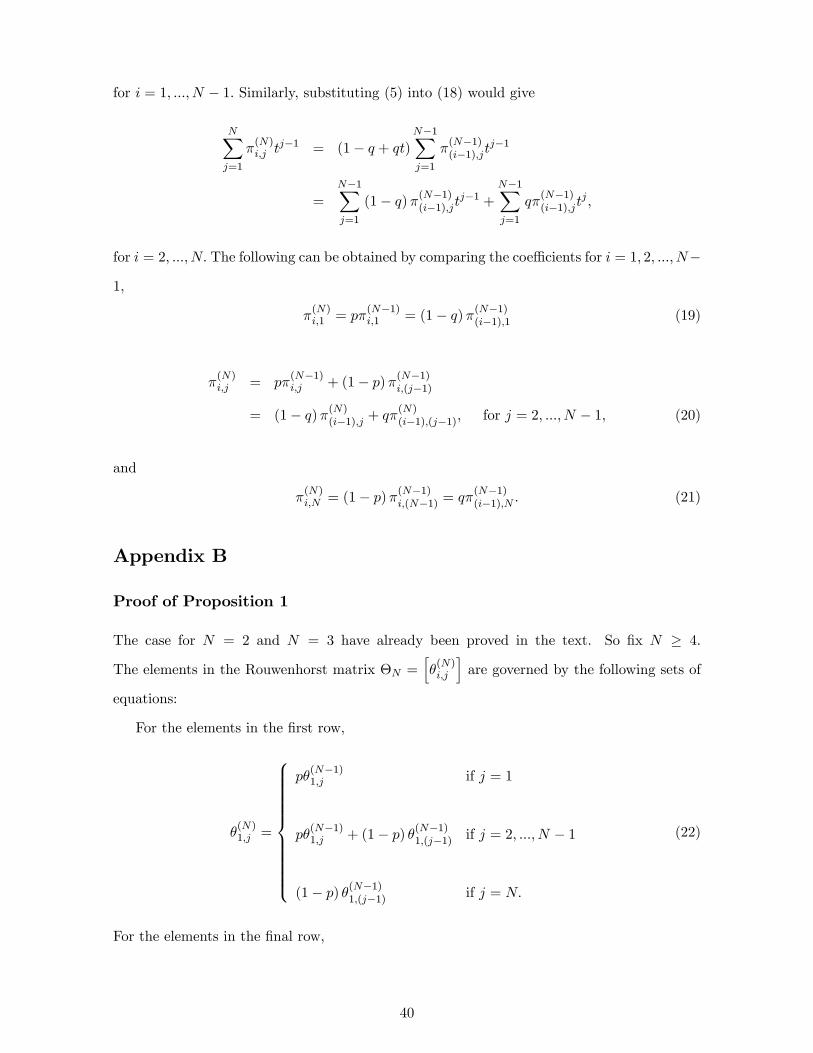
for i = 1; :::; N � 1: Similarly, substituting (5) into (18) would give

NXj=1

�(N)i;j t

j�1 = (1� q + qt)N�1Xj=1

�(N�1)(i�1);jt

j�1

=N�1Xj=1

(1� q)�(N�1)(i�1);jtj�1 +

N�1Xj=1

q�(N�1)(i�1);jt

j ;

for i = 2; :::; N: The following can be obtained by comparing the coe¢ cients for i = 1; 2; :::; N�

1;

�(N)i;1 = p�

(N�1)i;1 = (1� q)�(N�1)(i�1);1 (19)

�(N)i;j = p�

(N�1)i;j + (1� p)�(N�1)i;(j�1)

= (1� q)�(N)(i�1);j + q�(N)(i�1);(j�1); for j = 2; :::; N � 1; (20)

and

�(N)i;N = (1� p)�(N�1)i;(N�1) = q�

(N�1)(i�1);N : (21)

Appendix B

Proof of Proposition 1

The case for N = 2 and N = 3 have already been proved in the text. So �x N � 4:

The elements in the Rouwenhorst matrix �N =h�(N)i;j

iare governed by the following sets of

equations:

For the elements in the �rst row,

�(N)1;j =

8>>>>>>>>>><>>>>>>>>>>:

p�(N�1)1;j if j = 1

p�(N�1)1;j + (1� p) �(N�1)1;(j�1) if j = 2; :::; N � 1

(1� p) �(N�1)1;(j�1) if j = N:

(22)

For the elements in the �nal row,

40

�(N)N;j =

8>>>>>>>>>><>>>>>>>>>>:

(1� q) �(N�1)(N�1);j if j = 1

(1� q) �(N�1)(N�1);j + q�(N�1)(N�1);(j�1) if j = 2; :::; N � 1

q�(N�1)(N�1);(j�1) if j = N:

(23)

For the elements in row i = 2; :::; N � 1;

�(N)i;j =

8>>>><>>>>:12

hp�(N�1)i;j + (1� q) �(N�1)(i�1);j

iif j = 1

12

h(1� p) �(N�1)i;(j�1) + q�

(N�1)(i�1);(j�1)

iif j = N;

(24)

and for j = 2; :::; N � 1;

�(N)i;j =

1

2

hp�(N�1)i;j + (1� p) �(N�1)i;(j�1) + (1� q) �

(N�1)(i�1);j

+q�(N�1)(i�1);(j�1)

i; (25)

For any given �N�1; the system of equations (22)-(25) de�nes a unique �N : Similarly, for

any given �N�1; the system of equations (15)-(21) de�nes a unique �N : Since �2 = �2; it

su¢ ce to show that the elements in �N generated by (15)-(21) satis�es the system (22)-(25).

Consider the �rst row (i.e., i = 1) in �N : According to (15),

�(N)11 = pN�1 = p�

(N�1)11 ;

and

�(N)1;N = (1� p)

N�1 = (1� p)�(N�1)1;(N�1):

For j = 2; :::; N � 1; since

�(N�1)1;j =

�N � 2j � 1

�pN�1�j (1� p)j�1 ,

�(N�1)1;(j�1) =

�N � 2j � 2

�pN�j (1� p)j�2 ;

41

and �N � 1j � 1

�=

�N � 2j � 1

�+

�N � 2j � 2

�;

we have

�(N)1;j = p�

(N�1)1;j + (1� p)�(N�1)1;(j�1):

This shows that the elements in the �rst row of �N satis�es (22). Using (16) and the same

procedure, one can show that the elements in the last row of �N satis�es (23).

The rest of the proof follows immediately from (19)-(21). For any row i = 2; :::; N � 1 in

�N ; (19) implies

�(N)i;1 =

1

2

hp�

(N�1)i;1 + (1� q)�(N�1)(i�1);1

i:

Similarly, (20) and (21) imply

�(N)i;N =

1

2

h(1� p)�(N�1)i;(N�1) + q�

(N�1)(i�1);N

i;

and

�(N)ij =

1

2

hp�

(N�1)ij + (1� p)�(N�1)i;(j�1) + (1� q)�

(N�1)(i�1);j

+q�(N�1)(i�1);(j�1)

i; (26)

for j = 2; :::; N � 1; respectively. Thus all the elements in row i = 2; :::; N � 1 in �N satis�es

(24) and (25). This completes the proof.

Proof of Lemma 2

It su¢ ce to check that all the elements of �N are strictly positive. From (15) and (16), it is

obvious that the elements in the �rst and the last rows are strictly positive. For the other

rows, a simple induction argument is used. First, �2 is a stochastic matrix with non-zero

entries. Suppose the result is true for N � 1 � 2: It follows from (19)-(21) that �(N)ij > 0 for

i = 2; :::; N � 1 and for j = 1; 2; :::; N: This completes the proof.

42

Proof of Proposition 4

As mentioned in the proof of Proposition 1, the �rst column of �N is given by

�(N)i;1 = pN�i (1� q)i�1 ;

for i = 1; 2; :::; N: De�ne b�(N)i as in (6). Then

NXi=1

b�(N)i �(N)i;1 =

NXi=1

�N � 1i� 1

�sN�i (1� s)i�1 pN�i (1� q)i�1

=

NXi=1

�N � 1i� 1

�(sp)N�i (1� s)i�1 (1� q)i�1

= [sp+ (1� s) (1� q)]N

= sN = b�(N)1 :

For all other columns except the �rst one, an induction argument is used to prove the

result. As mentioned in the text, the guess is correct when N = 2: Suppose the guess is

correct for some N � 2; i.e.,

b�(N)j =NXi=1

b�(N)i �(N)i;j ; for j = 1; 2; :::; N: (27)

We have already proved that this is true when j = 1; so proceeds to j = 2; :::; N + 1:

Using (6), the following can be derived

b�(N+1)i =

8>>>><>>>>:sb�(N)i for i = 1

sb�(N)i + (1� s) b�(N)i�1 for i = 2; :::; N;

(1� s) b�(N)i�1 for i = N + 1:

(28)

43

Using these one can obtain

N+1Xi=1

b�(N+1)i �(N+1)i;j

= b�(N+1)1 �(N+1)1;j +

NXi=2

b�(N+1)i �(N+1)i;j + b�(N+1)N+1 �

(N+1)(N+1);j

= sb�(N)1 �(N+1)1;j +

NXi=2

hsb�(N)i + (1� s) b�(N)i�1

i�(N+1)i;j + (1� s) b�(N+1)N �

(N+1)(N+1);j

=NXi=1

sb�(N)i �(N+1)i;j +

N�1Xi=1

(1� s) b�(N)i �(N+1)(i+1);j + (1� s) b�(N+1)N �

(N+1)(N+1);j

=

NXi=1

sb�(N)i �(N+1)i;j +

NXi=1

(1� s) b�(N)i �(N+1)(i+1);j : (29)

Based on (20), the following can be obtained

�(N+1)i;j = p�

(N)i;j + (1� p)�(N)i;j�1;

and

�(N+1)i+1;j = (1� q)�(N)i;j + q�

(N)i;(j�1);

for j = 2; 3; :::; N: Substituting these into (29) gives

N+1Xi=1

b�(N+1)i �(N+1)i;j

= s

NXi=1

b�(N)i

hp�

(N)i;j + (1� p)�(N)i;(j�1)

i+ (1� s)

NXi=1

b�(N)i

h(1� q)�(N)i;j + q�

(N)i;(j�1)

i= [sp+ (1� s) (1� q)]

NXi=1

b�(N)i �(N)i;j + [s (1� p) + (1� s) q]

NXi=1

b�(N)i �(N)i;(j�1):

Using the induction hypothesis (27), the following can be obtained

N+1Xi=1

b�(N+1)i �(N+1)i;j = [sp+ (1� s) (1� q)] b�(N)j + [s (1� p) + (1� s) q] b�(N)j�1

= sb�(N)j + (1� s) b�(N)j�1

= b�(N+1)j ;

44

for j = 2; 3; :::; N: The last line is obtained by using (28). SincePN+1

i=1b�(N+1)i = 1 andPN+1

j=1 �(N+1)i;j = 1; the remaining equation

N+1Xi=1

b�(N+1)i �(N+1)i;j = b�(N+1)j ; for j = N + 1;

must be satis�ed. This completes the proof.

Appendix C

The objective of this section is to derive the moments listed on Table 1. Since it is under-

stood that these are moments for an N -state Markov chain, the notations �(N)i;j and �(N)j are

simpli�ed to become �i;j and �j ; respectively.

Preliminaries

The following result is used in deriving the conditional mean for the Markov chain.

Lemma 5 For any N � 2; and for i = 1; :::; N;

NXj=1

�i;j (j � 1) = (1� p) (N � i) + (i� 1) q; (30)

NXj=1

�1;j (j � 1)2 =

24 NXj=1

�i;j (j � 1)

352 + (N � i) (1� p) p+ (i� 1) q (1� q) : (31)

Proof. Recall the following expression

[p+ (1� p) t]N�i (1� q + qt)i�1 =NXj=1

�i;jtj�1; (32)

for i = 1; :::; N: Equation (30) can be obtained in two steps: (i) Di¤erentiate both sides of

(32) with respect to t: (ii) Set t = 1:

45

Equation (31) can be obtained as follows: Fix i = 1; :::; N: Di¤erentiate both sides of (32)

with respect to t twice and set t = 1. This gives

NXj=1

�i;j (j � 1) (j � 2) =

NXj=1

�i;j (j � 1)2 �NXj=1

�i;j (j � 1)

= [(N � i) (1� p) + (i� 1) q]2 � (N � i) (1� p)2 � (i� 1) q2

=

24 NXj=1

�i;j (j � 1)

352 � (N � i) (1� p)2 � (i� 1) q2:

Equation (31) can be obtained by combining this and equation (30). This completes the proof

of Lemma 5.

The following equations are useful in deriving the other moments. For a binomial distri-

bution with parameters N � 1 and 1� s; the �rst two moments are given by

NXi=1

�N � 1i� 1

�sN�i (1� s)i�1 (i� 1) = (N � 1) (1� s) ; (33)

NXi=1

�N � 1i� 1

�sN�i (1� s)i�1 (i� 1)2

= (N � 1) (1� s) s+ (N � 1)2 (1� s)2 : (34)

Conditional Mean

We are now ready to compute the conditional means. Conditional on yt = yi; the mean value

of yt+1 is given by

E (yt+1jyt = yi) =

NXj=1

�i;jyj =

NXj=1

�i;j

�� + 2

N � 1 (j � 1)�

= � + 2

N � 1

NXj=1

�i;j (j � 1) :

It follows from (30) that

NXj=1

�i;j (j � 1) = (1� p) (N � i) + (i� 1) q

= (1� p) (N � 1) + (q + p� 1) (i� 1) :

46

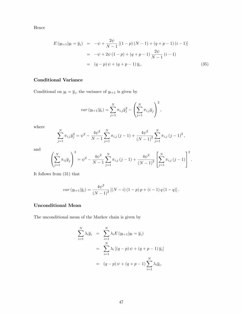
Hence

E (yt+1jyt = yi) = � + 2

N � 1 [(1� p) (N � 1) + (q + p� 1) (i� 1)]

= � + 2 (1� p) + (q + p� 1) 2

N � 1 (i� 1)

= (q � p) + (q + p� 1) yi: (35)

Conditional Variance

Conditional on yt = yi; the variance of yt+1 is given by

var (yt+1jyi) =NXj=1

�i;jy2j �

0@ NXj=1

�i;jyj

1A2 ;where

NXj=1

�i;jy2j = 2 � 4 2

N � 1

NXj=1

�i;j (j � 1) +4 2

(N � 1)2NXj=1

�i;j (j � 1)2 ;

and 0@ NXj=1

�ijyj

1A2 = 2 � 4 2

N � 1

NXj=1

�i;j (j � 1) +4 2

(N � 1)2

24 NXj=1

�i;j (j � 1)

352 :It follows from (31) that

var (yt+1jyi) =4 2

(N � 1)2[(N � i) (1� p) p+ (i� 1) q (1� q)] :

Unconditional Mean

The unconditional mean of the Markov chain is given by

NXi=1

�iyi =

NXi=1

�iE (yt+1jyt = yi)

=NXi=1

�i [(q � p) + (q + p� 1) yi]

= (q � p) + (q + p� 1)NXi=1

�iyi:

47

HenceNXi=1

�iyi =(q � p) 2� (p+ q) � �: (36)

Unconditional Second Moment

NXi=1

�iy2i =

NXi=1

�i

�� + 2

N � 1 (i� 1)�2

=

NXi=1

�i

� 2 � 4 2

N � 1 (i� 1) +4 2

(N � 1)2(i� 1)2

�

= 2 � 4 2

N � 1

NXi=1

�i (i� 1) +4 2

(N � 1)2NXi=1

�i (i� 1)2 :

Using (33) and (34), we have

NXi=1

�iy2i = 2 � 4 2 (1� s) + 4

2 (1� s) sN � 1 + 4 2 (1� s)2

= 2�1� 4 (1� s) s+ 4 (1� s) s

N � 1

�:

First-order Autocovariance

First consider the following expression,

E (ytyt+1) =NXi=1

�iE (yt+1ytjyt = yi)

=NXi=1

�iyiE (yt+1jyt = yi) :

Using (35), we have

E (ytyt+1) =

NXi=1

�iyi [(q � p) + (q + p� 1) yi]

= (q � p) NXi=1

�iyi + (q + p� 1)NXi=1

�iy2i : (37)

48

Let �2y be the unconditional variance of the Markov chain so that

�2y =NXi=1

�iy2i � �2;

where � is the unconditional mean de�ned in (36). Substituting this into (37) gives

E (ytyt+1)

= (q � p) �+ (q + p� 1)��2y + �

2�

= [(q � p) + (q + p� 1)�]�+ (q + p� 1)�2y;

where

(q � p) + (q + p� 1)� = (q � p) 2� (p+ q) = �:

Hence

E (ytyt+1) = �2 + (q + p� 1)�2y:

Thus the �rst-order autocovariance is given by

E [(yt � �) (yt+1 � �)] = E (ytyt+1)� �2 = (q + p� 1)�2y:

49

References

[1] Adda, J., Cooper, R., 2003. Dynamic Economics: Quantitative Methods and Applica-

tions. MIT Press, Cambridge, MA.

[2] Aruoba, S., Fernández-Villaverde, J., Rubio-Ramírez, J., 2006. Comparing Solution

Methods for Dynamic Equilibrium Economies. Journal of Economic Dynamics and Con-

trol 30, 2477-2508.

[3] Burnside, C., 1999. Discrete State-Space Methods for the Study of Dynamic Economies.

In: Marimon, R., Scott, A. (Ed.), Computational Methods for the Study of Dynamic

Economies. Oxford University Press, Oxford, 95-113.

[4] Davis, P.J., Rabinowitz, P., 1984. Methods of Numerical Integration 2nd Ed. Academic

Press, Orlando, FL.

[5] Flodén, M., 2008. A Note on the Accuracy of Markov-chain Approximations to Highly

Persistent AR(1) Processes. Economic Letters 99, 516-520.

[6] King, R.G., Rebelo, S.T., 1999. Resuscitating Real Business Cycles. In: Taylor, B.J.,

Woodford, M. (Ed.), Handbook of Macroeconomics, Volume 1. Elsevier, Amsterdam,

927-1007.

[7] Lkhagvasuren, D., Galindev, R., 2008. Discretization of Highly-Persistent Correlated

AR(1) Shocks. Unpublished manuscript, Concordia University.

[8] Lucas, R.E., 1978. Asset Prices in an Exchange Economy. Econometrica 46, 1429-1445.

[9] Rouwenhorst, K.G., 1995. Asset Pricing Implications of Equilibrium Business Cycle Mod-

els. In: Cooley, T.F. (Ed.), Frontiers of Business Cycle Research. Princeton University

Press, Princeton, NJ, 294-330.

[10] Tauchen, G., 1986. Finite State Markov-chain Approximations to Univariate and Vector

Autoregressions. Economic Letters 20, 177-181.

[11] Tauchen, G., 1990. Solving the Stochastic Growth Model by using Quadrature Methods

and Value-Function Iterations. Journal of Business and Economic Statistics 8, 49-51.

50

[12] Tauchen, G., Hussey, R., 1991. Quadrature-Based Methods for Obtaining Approximate

Solutions to Nonlinear Asset Pricing Models. Econometrica 59, 371-396.

[13] Taylor, J., Uhlig, H., 1990. Solving Nonlinear Stochastic Growth Models: A Comparison

of Alternative Solution Methods. Journal of Business and Economic Statistics 8, 1-18.

51