munerical md rhhlytical lumomrssi …f f, dimensionless stream function in navier-stokes equations f...
TRANSCRIPT

1I 13 THE MUNERICAL MD RhhLYTICAL STUDY' OF UZFURRTION IND /INULTICELLULAR FLO.. (U) RIR FORCE INST OF TECNNRIGNT-PATTERSON Fl ON D 9 FANT 1987
LUMOMRSSI FIEFTClI/NR-S7-13DF/G 29/0 L
mEEEEEEEh h

* - - . a. St a a - - - - S - - -
*1
ISII
IS.
'S.
.5..
SI'S
55
p.-I.-.
-S-p...
Hit j*~~ 128flit ,~ *32 WM'2
13611111 L* L..
lAO
* II IIItI~'~H1 ''
'p
-S
-S.5I.
-S
'4-
* -S-S
4 -S* -S
.~ ~v P1 ~ .d* -. . -. .P. . .5 ~

111AIASS I FLH'~~~ ~SECURITY CLASSIFICATION OF THIS PAGE (When Data ' nlere) __________________
REPORT DOCUMENTATION PAGE READ___ INSTRUCTIONS __
I. REPORT NUMBER 2. GOVT ACCESSION No. 3. RECIPIE CMPFTNU FOR
AFLT/CI/NR 87- 134D/.ff T fNUBRi1I
4. TITLE (and Subtitle) S. TYPE OF REPORT & PERIOD COVERED
The Numerical and Analytical Study of Bifurcatior~$SDSETTOand Multicellular Flow Instability Due to_______________Natural Convection Between Narrow Horizontal 6. PERFORMING OIG. REPORT NUMBER
Isothermal Cylindrical Annuli at High Rayleigh Nimbers7. ~ AU THOR(&) S. CONTRACT OR GRANT NUMBER(s)
00 Daniel Bartholemew Fant
9. PERFORMING ORGANIZATION NAME AND ADDRESS 10. PROGRAM ELEMENT. PROJECT. TASK
AFIT TUDEN AT:AREA & WORK UNIT NUMBERS
Iowa State University _______________It. CONTROLLING OFFICE NAME AND ADDRESS 12. REPORT DATE
AFIT/NR 1987WPAFB OH 45433-6583 13. NUMBER OF PAGES
25114. MONITORI-1NG AGENCY NAME 8 ADDRESS(i( different from Cotitroiiing Office) 1S. SECURITY CLASS. (of this repot)
UNCLASSIFIED15a. DECLASSIFICATION/ DOWNGRADING
SCHEDULE
16. DISTRIBUTION STATEMENT (of this Report)
*APPROVED FOR PUBLIC RELEASE; DISTRIBUTION UNLIMITED DI
17. DISTRIBUTION STATEMENT (of the abstract entered In Block 20, It different fromt Report)
il. SUPPLEMENTARY NOTES
*APPROVED FOR PUBLIC RELEASE: IAW AFR 190-1 r
Iarf Research an'Professional Development
AFIT/NR19. KEY WORDS (Continue on reverse side If necessary and Identify by block number)
20. ABSTRACT (Continue on reverse side It necessary aid Identify by block number)
ATTACHED
DD I1JAN 73 1473 EDITION OF I NOV65 IS OBSOLETE
SECURITY CLASSIFICATION OF THIS PAGE (07ven Plato Entered)

The numerical and analytical study of bifurcation and multicellular
flow instability due to natural convection between narrow horizontal
isothermal cylindrical annuli at high Rayleigh numbers
Daniel Bartholemew Fant
Under the supervision of Joseph M. PrusaFrom the Department of Mechanical Engineering
Iowa State University
This-restafcIffort deals with a numerical and analytical study
of multicellular flow instability due to natural convection between
narrow horizontal isothermal cylindrical annuli.
Buoyancy-induced steady or unsteady flow fields between the annuli
are determined using the Boussinesq approximated two-dimensional (2-0)
Navier-Stokes equations and the viscous-dissipation neglected thermal-
energy equation. The vorticitystream function formulation of the
NavierJStokes equations is adopted.
Both thermal and hydrodynamic instabilities are explored. An
asymptotic expansion theory is applied to the Navier-Stokes equations in
the double-limit of Rayleigh number approaching infinity and gap width
approaching zero. This double-limiting condition reduces the governing
equations to a set of Cartesian-like boundary-layer equations. These
equations are further simplified by considering the extreme limits of .
Pr * and Pr - 0. The former limit yields an energy equation which 0"
retains the nonlinear convective terms, while the vorticity equation ................:
reduces to a Stokes-flow equation, signifying the potential for thermal
instability. In the latter limit, the nonlinear terms in the vorticity, D.1*
OPY0%

equation remain, while the energy equation collapses to a one-dimensional
conduction equation, signifying the potential for hydrodynamic
instability.
Thermal instability of air near the top portions of narrow annuli
is considered for various size small gap widths. For these narrow gaps,
the Rayleigh numbers corresponding to the onset of steady multicellular
flow are predicted. Numerical solutions of the 2-0 Navier-Stokes
equations also yield hysteresis behavior for the two-to-six and two-to-
four cellular states, with respect to diameter ratios of 1.100 and 1.200.
In contrast, an unsteady hydrodynamic multicellular instability is
experienced near the vertical sections of narrow annuli when the Pr - 0
boundary-layer equations are solved numerically.
In addition, analytical steady-state perturbative solutions to the
boundary-layer equations are obtained. These results compare favorably
to related numerical solutions of both the Navier-Stokes and the Pr - 0
simplified equations.
In all cases, finite-differenced solutions to the governing
equations are obtained using a stable second-order, fully-implicit
time-accurate Gauss-Seidel iterative procedure.
J 4: X'? 4 i < - - ; L ; ';. ,: , : : :

ii
TABLE OF CONTENTS
Page
NOMENCLATURE v
1. INTRODUCTION 1
2. LITERATURE REVIEW 3
2.1. Analytical Studies 4
2.2. Experimental Studies 13
2.2.1. Heat transfer correlations 19
2.3. Numerical Studies 23
2.4. Variable Fluid Properties 33
2.5. Flow Bifurcation 35
2.6. Natural Convection in Vertical Slots 39
2.7. Concluding Remarks 44
3. MATHEMATICAL ANALYSIS 46
3.1. The Physical Model 46
3.2. The Complete Set of Governing Equations 48
3.3. The Dimensional Formulation 49
3.3.1. Governing equations in primitive variables 493.3.2. Governing equations using the stream
function-vorticity approach 523.3.3. Boundary conditions 553.3.4. Initial conditions 57
3.4. The Dimensionless Formulation 57
3.4.1. Coordinate transformation 583.4.2. Governing equations 583.4.3. Boundary conditions 633.4.4. Initial conditions 63
4. ASYMPTOTIC ANALYSIS 65
4.1. The Inviscid Core 66
.-.'.. %- ' ..,'- ' " -. .. %... .. - ... . - v-,.,-' .-w ... . ... -& . 2-,.. - -. .-.-.-... J-., .. ,.

iii '
Page
4.2. The Boundary-Layer Expansion 70
4.3. The Analytical Cell-Development Regime 74
4.4. The Perturbative Solution to the Steady-StateFinite-Prandtl Number Equations 78
4.4.1. Heat transfer relations 85
4.5. The Zero Prandtl Number Limit 87
4.6. The Perturbative Solution to- the Steady-StateZero Prandtl Number Equations 92
4.7. The Infinite Prandtl Number Limit 97
5. NUMERICAL ANALYSIS 103
5.1. The Numerical Method of Solution 104
5.1.1. Variable increment finite-differenceformulas 106
5.1.2. Finite-difference equations for thedependent variables 108
5.1.2.1. 2-D Navier-Stokes equations 1085.1.2.2. Finite-Prandtl number boundary-
layer equations 1135.1.2.3. Zero-Prandtl number boundary-
layer equations 118
5.1.3. Boundary conditions 120
5.1.3.1. 2-D Navier-Stokes equations 1205.1.3.2. Finite-Prandtl and Zero-
Prandtl number equations 123
5.2. The Computational Procedure 124
5.2.1. Iteration sequence and convergencecriterion 125
5.2.2. Relaxation parameters 1265.2.3. Multicellular flow determination 1285.2.4. Computational details and discussion 129
6. RESULTS AND DISCUSSION 136
6.1. Thermal Instability 136
, '," ' - ,Ze Z 'Z j,''.' . ." ,, . ,/./ "... ' '"' -, '. t', . .' " "" ,'.'. ' '- \'. ". '. '" , -""1"

iv
Page
6.1.1. Hysteresis behavior 1366.1.2. Analytical comparison 1546.1.3. Small-gap number stability curves 160
6.2. Hydrodynamic Instability 163
6.2.1. Pr - 0 numerical solution 1656.2.2. Pr - 0 perturbative solution 1876.2.3. Small-Prandtl number stability curves 196
7. CONCLUSIONS 204
8. REFERENCES 208
9. ACKNOWLEDGMENTS 219
10. APPENDIX A: ANALYTICAL COEFFICIENTS 220
11. APPENDIX B: LIMITING CONDITIONS OF THE 2-DNAVIER-STOKES EQUATIONS 224
11.1. The Pr - 0 Equations 224
11.2. The Pr - - Equations 227
12. APPENDIX C: En VERSUS En+l FORMULATION 231
12.1. En Truncation - Error Analysis 231
12.2. Numerical Comparison of En Versus En+l 235
13. APPENDIX D: HEAT TRANSFER AND SHEAR STRESSRELATIONS 238
13.1. Dimensionless Nusselt Numbers 238
13.2. Dimensionless Shear Stresses 239
13.3. Heat Transfer and Shear Stress Finite-Difference Expressions 240
14. APPENDIX E: TRUNCATION-ERROR STUDY 244
14.1. Upwind Versus Central - Differencing 244
14.2. Mesh Resolution Study 246
14.3. Mean Nusselt Number Correlations 250

V
NOMENCLATURE
a Inner cylinder radius
b Outer cylinder radius
c Specific heat
er Unit vector in radial direction
Unit vector in angular direction
f f, dimensionless stream function in Navier-Stokes
equations
f Dimensionless stream function in finite-Pr boundary-
layer equations
g g, acceleration of gravity
h Heat transfer coefficient
hb, hf Variable radial increments
k Thermal conductivity
kbpkblkf~kfl Variable angular increments
k Equivalent thermal conductivity (actual heat fluxeq divided by conductive heat flux)
p Pressure
q Local heat flux
r b-a dimensionless radial coordinater b-a
t dimensionless time in Navier-Stokes equationsa
t RaI/2 t, dimensionless scaled time in finite-Prboundary-layer equations
Ra 1/2t (-) t, dimensionless scaled time in zero-Pr
boundary-layer equations
*% a.aa~aa1J5V.;.%.~a~. ~ ~ a~' ~aa-a
vi
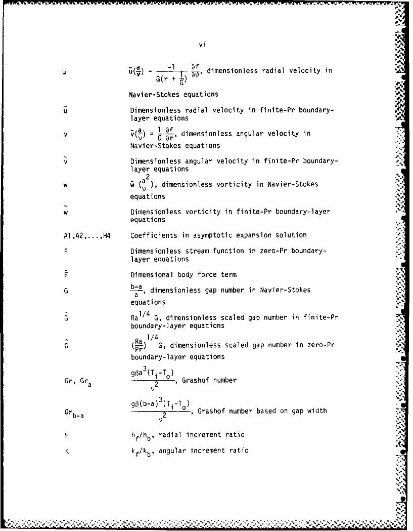
u 7-, dimensionless radial velocity inVaye G(r + )
Navier-Stokes equations
u Dimensionless radial velocity in finite-Pr boundary-layer equations
w (! =( --- , dimensionless angular velocity in
Navier-Stokes equations
v Dimensionless angular velocity in finite-Pr boundary-layer equations
w (L-), dimensionless vorticity in Navier-StokesV
equations
w Dimensionless vorticity in finite-Pr boundary-layerequations
Al,A2,...,H4 Coefficients in asymptotic expansion solution
F Dimensionless stream function in zero-Pr boundary-layer equations
Dimensional body force term
G b-a dimensionless gap number in Navier-Stokes
equations V
G Ra1/4 G, dimensionless scaled gap number in finite-Prboundary-layer equations
1/4G (-) G, dimensionless scaled gap number in zero-Pr Ol
Prboundary-layer equations
ga 3 (T -To )Gr, Gr 2 , Grashof number
a 2
gs(b-a) 3(Ti-T 0 )Grba 2 , Grashof number based on gap width
H hf/hb, radial increment ratio
K kf/kb, angular increment ratiof b9

vii
NR Number of nodes in radial direction
NS Number of nodes in angular direction
Nu qa/{k(Ti-T )}, local Nusselt number
Nu Mean Nusselt number
Nb} -1, conductive Nusselt numberNUCOND a(n
P, Q Dummy variables
Pr v/c, Prandtl number
R -a/S, stretched inner radial coordinate
ga 3(Ti-T )Ra V 10, Rayleigh number
RATR Rayleigh number characterizing the onset ofmulticellular transition
Rab~a 1) , Rayleigh number based on gap width
S Source term in numerical method
T-T o
T -, dimensionless temperature in Navier-StokesT i T To
equations
T Dimensionless temperature in finite-Pr boundary-
layer equations
Ti Inner cylinder temperature
T Outer cylinder temperatureo
W Dimensionless vorticity in zero-Pr boundary-layerequations
D/Dt Total time derivative

viii
Greek symbols
k thermal diffusivity
Coefficient of thermal expansion
Boundary-layer thickness
S Convergence criterion, or dimensionless eccentricityvariable
a T-a-, dimensionless local shear-stress14.
Y Dimensionless average shear-stress
xParameter in finite-difference equations
IDynamic viscosity, or parameter in finite-differenceequation
v -, momentum diffusivityP
i, dimensionless angular coordinate
p Density
TLocal shear-stress, or time increment in numericalmethod
Arbitrary dependent variable
r Parameter in finite-difference equations
Q1' Q2 Relaxation parameters in numerical method
V Gradient differential operator
VI,V2,V Parameters in finite-difference equations
V2, 2 Second-order differential operators
' r F

ix
Superscripts
m Iteration number
n Time level
Subscripts
BL Boundary-layer
c Inviscid-core
i Radial position, or heated inner cylinder surface
j Angular position
o Cooled outer cylinder surface
O,,,,8,10,12 Node position in computational molecule
0,1,2,3,4 Order of expansion term in asymptotic analysis
%9
- ~ ~ , -- -

1. INTRODUCTION
From a practical standpoint, the study of natural conrec",
between horizontal isothermal concentric cylinders has a wi e
of technological applications, ranging from nuclear reactors arc
thermal storage systems to cooling of electronic components, a'r r'
fuselage insulation, underground electrical transmission lines arc er
the flow in the cooling passages of turbine blades (Tsui and Tremblay,
1984).
However, in a different perspective, the work set forth in this
research effort was undertaken to gain a more practical understanding
of the effects of nonlinearity with regard to natural convective flow
instabilities. Still not well understood is the influence of Orandtl
number variations on the nonlinear processes involved in triggering
either thermal or hydrodynamic types of instabilities. Also of
relevance is the aspect of nonuniqueness, which allows the possibility
of hysteresis behavior associated with thermal-convective
instabilities. These important issues and concerns are addressed and
studied in this thesis.
In light of the above, the work in this thesis is separated into
three main areas.
First, a stable second-order finite-difference solution to the
2-D Navier-Stokes equations is implemented in order to investigate
possible hysteresis behavior in relation to multicellular thermal
instability near the top of narrow horizontal annuli for air.
A r -
. -. I

2
The second area of work involves an asymptotic expansion theory
applied to the 2-D Navier-Stokes equations in the double-limit of
Rayleigh number approaching infinity and gap width approaching zero. ,
In this double-limit, the Navier-Stokes equations are reduced to
Cartesian-like boundary-layer equations. Analytical steady-state
solutions to these simplified equations are also obtained, and the
results are compared to related 2-D Navier-Stokes numerical data.
Moreover, in order to obtain further insight into the nonlinearity
associated with extreme Prandtl number variations, limiting boundary-
layer equations for Pr - 0 and Pr are derived.
Thirdly, the Pr - 0 simplified boundary-layer equations are
solved numerically to investigate the full effects of nonlinearity,
which were believed to cause an unsteady hydrodynamic multicellular
instability between the vertical portions of narrow horizontal annuli.
Before delving into deep analysis and discussion of these topics,
an intensive literature review and derivation of the applicable
governing equations are presented in Chapters 2 and 3, respectively.
Finally, the key results and conclusions of this work are given in
Chapters 6 and 7.
de
%.

3
2. LITERATURE REVIEW
Natural convection phenomena between horizontal isothermal
concentric cylinders have been scrutinized experimentally, analytically,
and numerically throughout the past few decades. In the 1960s, most
work was experimental in nature. In the '70s and '80s, many numerical
studies dominated the literature due to the advent of the modern computer.
Analytical studies, in general, have been much more limited.
This thesis concentrates on the high Rayleigh number/small-gap
flow regime. It has been found that while numerical studies in the low
to moderate Rayleigh number range are quite abundant and agree rather
favorably with related experimental work, the numerical work in the
high Rayleigh number multicellular flow regime (usually associated with
narrow gaps) has been much less exhaustive. This is due to the fact
that many computational schemes either could not resolve the transition
to the laminar multicellular flow field, or they became unstable just
prior to it. Analytical approaches, especially with regard to the
high Rayleigh number/small-gap flow regime, have been virtually
unexplored.
To better understand how the various studies were conducted and
evolved, this literature survey will be essentially divided into three
main categories; namely, the analytical analyses, the experimental
approaches, and the numerical studies. In addition, three sections will
be included near the end of this chapter to further support some of the
assumptions and findings relevant to this present study. These
- . - ' . . Sd .. d

4
sections will touch upon variable fluid property effects, flow
bifurcation, and natural convective flow between vertical slots.
Although many of the reviews will relate to the pretransition, non-
multicellular flow studies, their inclusion is necessary to fully
appreciate some of the follow-up work described in this thesis.
The basic flow field normally encountered between horizontal
isothermal concentric cylinders (see Figure 6.3a) is the bicellular
kidney-shaped pattern that results strictly from buoyancy effects:
density differences occur due to the inner cylinder being hotter than
the outer one. The lighter, hotter fluid begins to rise in a boundary-
layer manner near the warmer inner cylinder while ascending more
uniformly in the inviscid core region near the center of the annulus.
Finally, it separates and impinges upon the top of the outer cylinder
via the thermal plume. The cooler, more dense fluid, then, descends
along the outer cylinder and regains its upward cyclic ascent near the
lower oortion of the annulus. A similar kidney-shaped flow pattern will
also occur when the inner cylinder is cooled and the outer one heated.
Other interesting flow patterns are possible and will be discussed in
the sections that follow. Symbols will be either directly defined or
their meaning may be found in the Nomenclature.
2.1. Analytical Studies
Eight analytical studies pertaining to natural convective flow
between horizontal concentric cylinders were found in the literature
search. Of the eight, seven involved perturbation methods and only
%N

-7 ...- - , 'rVvvy'w
5
one dealt with linearized stability theory. All but one related to the
relatively small Rayleigh number domain.
Mack and Bishop (1968) used a Rayleigh number power series
expansion to obtain a steady-state solution for natural convection
between 2-D horizontal isothermal cylinders. The dimensionless
vorticity-transport and energy equations were assumed to govern the flow
field in this analysis. They eioanded temperature (T) and the stream
function (') in the following mf,'ier:
T E AJTj(r,e) (2.1a)
j=O
= AJ4j(r,e) (2.1b)j=l
where A signified the Rayleigh number and G the angular coordinate.
The first term in their expansion represented the creeping-flow
solution and was in agreement with that obtained by Crawford and
Lemlich (1962). The expansions for temperature and stream function
were carried out to three terms. It was estimated that for Pr - 1,
the convection terms were negligible in comparison to the conduction
terms for Rayleigh numbers ranging up to approximately 104 and R (the
radius ratio) in the range of 1.15 to 4.15. Vertical symmetry was
assumed, and for Pr > 1, the flow resulted in the single-cell kidney-
shaped pattern for moderate Rayleigh numbers. But for A ~ 0 (104), the
second and third terms in the stream function expansion started to
outgrow the first term, so any resulting flow patterns were deemed
,owe~~V I-*.Ct'F%

6
invalid. For the case of Pr .02 (liquid mercury), A : 300 and
R = 2.0, a multicellular flow was reported. Two weak secondary cells
formed at the top and bottom, while a stronger primary cell formed near
the center of the annulus. At the time though, experimental results for
the larger gap low-Prandtl number range were unavailable; hence, their
multicellular flow pattern could not be fully supported. Note that a
similar perturbation analysis was performed for spherical annuli in
Mack and Hardee (1968). Their flow field patterns were very similar
to those obtained in the concentric cylinder geometry.
Rotem (1972) studied the conjugate problem of conduction within
the inner cylinder coupled with convective motion in the gap. Through
a trial-and-error procedure, he was able to obtain the following
expansions for stream function and temperature:
= G G 2,a + Pr G 3 + PrGb
W i 1 GP 2+PG 2 3 3
+ Pr2 G3 c + .... (1 < r < R) (2.2a)3
T = To + RT+RGTa 2RAl A2+ RAT2 b + RAGT3 + .... (2.2b)
where G was the Grashof number based on (R-l), RA represented the
Rayleigh number, and R the outer-to-inner radius ratio. The first term
in these expansions corresponded to the creeping-flow solution.
Rotem (1972) carried out the stream function expansion to two terms
and calculated three terms for the temperature perturbation expansion.
.f , ;' .'.i ,- [" ; ".'-.-.. ' -. .- . :.,. -. -p

7
Through his results, Rotem (1972) confirmed the basic single-cell
solution and reinforced the idea that one should be careful in reporting
counter-rotating cells with an asymptotic method, since this usually
signifies that the expansions are starting to diverge. He did not
investigate the extreme Prandtl number cases, but he did express the
fact that further transformations were needed to eliminate Pr as an
independent parameter and render the equations free from singularities
in the limits of Pr - 0 and Pr - o. Such has been obtained, for
example, in his analysis on natural convection above unconfined
horizontal surfaces (Rotem and Claassen, 1969).
Hodnett (1973) used a perturbation method to analyze the same
problem as Mack and Bishop (1968), except that his analysis was in
terms of primitive variables. He extended his work in order to determine
how large R could be, at a given value of Grashof number, for the
problem to remain conduction dominated. He found that convection was
negligible only when R satisified
R3 Zn-I R = O[(G)-l] (2.3)
where cG represented his Grashof number and c was given by
Ti - TO
T0
while G signified a natural convective type Reynolds number.

8
Huetz and Petit (1974) performed a theoretical study of free
convection in a horizontal annulus for low values of Grashof number.
Their governing equations were written in the same form as Mack and
Bishop (1968), and vertical symmetry was also assumed. They expanded
stream function and temperature in a power series with respect to
Grashof number (Gr), where Gr was based on the inner cylinder radius.
Two case studies were investigated. Case I related to a constant heat
flux imposed on the inner wall and constant temperature on the outer
wall, and vice-versa for case II. For Pr - 1, only monocellular flow
was obtained in both cases I and II, regardless of the radius ratio for
Grashof numbers less than 1,000. However, for Pr = .02, R = 2.0, and
Gr = 15,000 (or Ra = 300), a multicellular flow was observed. Secondary
cells formed at the top and bottom of the annulus with the primary cell
in the center, but the secondary cells did not appear simultaneously.
In case I, the bottom cell appeared first, and in case I, the upper
cell appeared first. Thus, the results of this study further support
the multicellular flow recognized by Mack and Bishop (1968).
Custer and Shaughnessy (1977a) investigated natural convection
within a horizontal annuli for very low Prandtl numbers by solving the
dimensionless thermal energy and vorticity equations with a double
perturbation expansion in powers of Grashof and Prandtl numbers. The
stream function and temperature expansions were written as:
)(r,) Z Pm rr,) (2.4a)n=o m=0 ro nm

W - ., f
.' '. , . ... . .0 , . -, -_ - -, ,* . -
9
T(r,e) E z Pr GrTroT k (r,e) (2.4b)j=0 k=0 0 j
For a fairly large gap of R = 5 and Pr - 0, they reported that the
center eddy fell downward as the Grashof number increased, which was
contrary to the behavior of fluids for Pr > .7. For this same size
gap, at Gr 12,000, they observed the formation of a weak eddy nearro0
the top of the inner cylinder. For R = 2, at Grro = 120,000, two weak
eddies formed near the top and bottom of the annulus while the
stronger kidney-shaped one remained in the center. Vertical symmetry
was again assumed for this problem. These conclusions also help to
confirm the multicellular flow pattern observed by Mack and Bishop
(1968). Custer and Shaughnessy also stressed that only numerical
solutions to the full nonlinear equations, or experiments, could
actually establish the true existence of this multicellular flow field.
Custer and Shaughnessy (1977b) continued to study the problem
described in the above review. In this analysis, the dependent
variables in the governing equations were represented by the following
partial spectral expansions:
Oo
7(r,3) = n (r) sin no (2.5a)n=l
T(r,o) nZ gn(r) cos no (2.5b)n.O

Ir .r , V. ; W. IV -l.1 "W v 1.: : - r-,V-W-%W -,,-- .
10
The use of these expansions resulted in ordinary differential equations
governing fn(r) and gn(r). The equations were solved numerically and
their results were based on the series being truncated after three
terms. For Pr = .01 and Ra < 50 (or Gr < 5,000), they obtained the
following correlation for their heat transfer data (note that Ra and Gr
were based on the inner cylinder radius):
at R = 2.00, keq = 1 + 5 x 10⁻⁸ Ra2 0 1 4 (2.6a)
at R = 4.00, keq = 1 + 1 x 10. 4 Ra1.935 , (2.6b)
where keq signifies the average equivalent thermal conductivity and
represents the actual mean heat flux divided by the heat flux for pure
conduction. For a radius ratio of 1.1, they found that k was equaleq
6to 1 out to a Grashof number of approximately 10 . Also, for all the
cases studied, only the single-cell flow field resulted in the vertical
half of the annulus.
Walton (1980) utilized a multiple-scales linearized stability
theory to study the instability of natural convective flow between
narrow cylindrical annuli. First, he represented the basic flow by
expanding the stream function (f')) and temperature (T) in terms of the
dimensionless gap width, c:
( ,T) 0 ,T0 ) + C(' lT + E2(2,T2) (2.7a)
. '....-._-.. . .. - .-. - -...-,.. . .. ... .... ..... , ...-..-.. ... . -. - - . d.o.- .'.-.-. .-.- - -

where
r- r.1 0 and l << 1 (2.7b)
ri
He then let ' and T' represent small perturbations to P and T given
in Eq. (2.7a). By using the dimensionless forms of the vorticity and
energy equations, he was able to consider the stability of the basic
flow to small disturbances, via linearized stability theory. He
determined that the convective flow became unstable at a critical value
of the Rayleigh number, R, (associated with a particular wavenumber)
given by:
R=R +eR + (2.8)
where, for Pr .7, Rc 1707.762 and R= 258.4. Thus, as c 0,
R - 1707.762. According to his results, the narrow-gap annulus
collapsed to the horizontal flat plate B~nard problem as the gap width
tended to zero. Hence, for Pr - 1, a thermal-type instability should
arise near the top of the annulus.
Jischke and Farshchi (1980) studied the boundary-layer regime for
laminar free convection between 2-D horizontal annuli at the large
Rayleigh number limit. They divided the flow field into five
physically distinct regions, valid for the high Rayleigh number
limiting condition. They assumed a stagnant regime for the bottom part
of the annulus; a boundary-layer type behavior near the inner and
outer cylinders; an inviscid core region in the center portion of the

12
annulus; plus a thermal plume section along the vertical line of
symmetry above the inner cylinder, where the inner boundary-layer joins
up with the outer boundary-layer. Their governing equations were
written in terms of primitive variables, and they employed a zeroth-order
asymptotic expansion to represent the velocity and temperature fields
within the annulus. For the boundary-layer regime, they assumed (from
free convective boundary-layer studies of a single horizontal cylinder)
that the velocity and temperature fields would scale as:
u Ra1/4
vv V 0 + ..
T T +.... (2.9)
where u signified the radial velocity and, v, the tangential velocity
component. Their simplified equations, resulting from the Ra -
limit, were solved by means of an integral method in the limit of
Pr - -. They compared their heat transfer results to those of Kuehn
and Goldstein (1976a) for a radius ratio of R = 2.6, Pr = .706 and
4Ra = 4.7 x 10 . Qualitatively, their basic flow field and results were
very similar, but significant deviation was apparent in their plots of
the variation of local Nusselt number with angular position on the
inner cylinder. Their best agreement was achieved near the top of the
inner cylinder, at e = 1800. They seemed to have captured the
essential features of the flow field in their boundary-layer analysis,
.9 " * ' ' ' ' ' ' ' ''-- . .. ... - - - ': u '
'" . ':'' - r" , , -• m -m , =

13
although only bicellular-type flows were studied. The authors of this
article did not investigate the narrow-gap limit of their Ra
equations.
2.2. Experimental Studies
Most of the articles in this section relate to natural convection
between either concentric cylinders or spheres. Various flow patterns
have been investigated in the experimental work, ranging from the
multicellular flow prevalent in the narrow gaps to the unsteady type
flows originating in the larger gaps. Studies include both 2-D and 3-D
phenomena over a range of fluids such as air, water, liquid mercury, oil
and glycerin.
Liu et al. (1962) studied natural convection heat transfer for air,
water and silicone oil (0.7 < Pr < 3,500) between horizontal
cylindrical annuli. They considered five different geometries with
radius ratios of R = 1.154, 1.5, 2.5, 3.75 and 7.5. For the larger
radius ratios, all three fluids experienced a slow sideways oscillation
near the top of the cylinders as the Rayleigh number (Rab-a) exceeded
some limiting value, and this valt.-. decreased with gap size. For the
smaller gap, R = 1.154, a multicellular type flow (near the top) was
observed for air and silicone oil, at Rab-a of approximately 2,000
and 18,000, respectively. A kidney-shaped flow pattern was maintained
below the counter-rotating cells that formed near the top of the
annulus. They speculated that for gaps smaller than R = 1.154, the
Bdnard critical Rayleigh number (Rab-a 1700) would be approached.
b-a
-p - . ~~ *% .. -. . . . . . . ~. . . .

I-
14
Bishop et al. (1964) investigated natural convective heat transfer
between concentric spheres. They examined two radius ratios, R = 3.14
and R = 1.19. For the larger gap, only the kidney-shaped flow pattern,
similar to that seen for concentric cylinders, was observed. No
sideways oscillations were noticed. But in the smaller gap, R = 1.19,
two counter-rotating cells appeared near the top at a Raba of about
3,600. However, due to the spherical geometry, the two secondary cells
almost immediately began to coalesce into an elongated shape and soon
became indistinguishable. Although the geometries are different,
the multicellular flow observed in the narrow spherical annuli supports
the same type of flow seen by Liu et al. (1962) in the narrow
cylindrical annuli.
Grigull and Hauf (1966) used a Mach-Zehnder interferometer to
measure the temperature field between horizontal cylindrical annuli
filled with air. From these measurements, they were able to obtain the
local Nusselt numbers for a particular gap size and Grashof number. They
discussed three different regimes of convective flow:
1. A 2-D pseudo-conductive regime for Gr < 2,400. Here,b-a
conduction effects were dominant, although some convective
motion was evident.
2. A transitional regime with 3-D convective motion, for
2,400 < Grb-a < 30,000. For the intermediate-size gaps,
(1.2 < R < 2.0), the flow field transitioned to a form of
3-D vortices in unsteady oscillatory motion.
% -.
I l i I " l' i I -'-'- .... " . .... . .. .... .. " " "

15
3. A 2-D fully-developed laminar convective motion regime
p for 30,000 < Grb-a < 716,000. The 2-D motion was considered
steady for the larger gap widths in this particular range of
Grashof numbers. They did notice that as Grashof number
increased, the centers of the kidney-shaped cells moved
closer to the upper portion of the annulus.
Vivid flow pictures (observed by cigarette smoke) were included for all
three convective flow regimes.
Bishop et al. (1966) extended their study of 1964 (Bishop et al.,
1964) to include the effects of various radius ratios, ranging from
R = 1.19 to R = 3.14. In their experiments, they confirmed the
occurrence of counter-rotating cells previously observed in the smallest
gap width, R = 1.19. For the relatively narrow gaps (slightly greater
than R = 1.19) in the high Grashof number range, they observed a
boundary-layer type flow near the walls of the annulus, coupled with a
slower, more uniform type of fluid motion near the center. Also, from
their measured heat-transfer data for four different radius ratios,
they obtained two Nusselt-Grashof number correlations that fit their
data to within 15.5 percent.
Lis (1966) studied the flow behavior in simple and obstructed
annuli using the Schileren technique with both sulphur hexafluoride
and nitrogen as the working fluid. The six axial spacers used in the
obstructed annuli provided for enhanced heat transfer effects (compared
to the simple annuli) due to more efficient mixing near the upper parts
of the annulus. Also, for 2 < R < 4, the flow pattern became unstable
16
at the higher Rayleigh numbers and random oscillations developed near
the top of the gap (for the unobstructed annuli).
Bishop and Carley (1966) performed photographic studies of natural
convective air patterns between concentric cylinders. They observed an
oscillatory flow for R = 3.69, that started at Raba 270,000 (a much
larger value than that indicated by Liu et al. (1962) for the same size
gap). They also tried to reproduce the multicellular flow field
observed by Liu et al. (1962) for the small gap, R = 1.154. They used
a gap width of .688 inches, and for Rayleigh numbers (Raba) up tob-a
20,000, no type of multicellular flow occurred. Either the gap size
was too large, or a much higher Rayleigh number was needed to observe
the cells with their particular apparatus.
Bishop et al. (1968) re-examined experimentally, for air, the
oscillatory flow in the larger size cylindrical annuli. For gap widths
of R 3.70, 2.46 and 1.846, they observed that the oscillations
started at Rayleigh numbers (Rab-a) of approximately 240,000, 150,000
and 35,000, respectively. Using the data from these three gaps, they
obtained empirical correlations for the period, wavelength and
amplitude of the oscillations.
Powe et al. (1969) experimentally studied the natural convective
flow of air between h'.rizontal concentric cylinders for various radius
ratios. They characterized the flow into three basic regimes:
1. 2-D multicellular flow for R < 1.2,
II. 3-D spiral flow for 1.2 < R < 1.7, and
III. 2-0/3-0 oscillatory flow for R > 1.7.
.o

17
Regimes II and III were unsteady. The multicellular flow field in
Regime I remained steady for a small number of cells, but as the
Rayleigh number increased and the chain of cells near the top stopped
forming, slight oscillations about the vertical center-line occurred.
Yin et al. (1973) experimentally investigated the natural
convective flow patterns between isothermal concentric spheres for air
and water. For air, with R = 1.4 and Rab-a = 5930, they observed two
steady counter-rotating cells near the top of the annulus. With the
larger gaps (R = 2.17 and 1.78), for both air and water, the familiar
kidney-shaped pattern resulted for relatively small Rayleigh numbers.
But as Rayleigh number increased, an unsteady flow behavior was
initiated.
Kuehn and Goldstein (1976a) studied the natural convective flow of ,
air and water between isothermal concentric cylinders both
experimentally and numerically. A Mach-Zehnder interferometer was used
to obtain temperature profiles for both air and water with an annulus
of R = 2.6. Heat transfer correlations were found by using a least-
squares regression analysis. For air,
S .159R 272 , 2.1 x 10⁴ < Ra < 9.6 x 10 (2.10)eq b-a b-a
and for water,
k =.234 Ra 2.3 x l0 < Ra < 9.8 x 10 (2.11)eq b-a b-a
4 . . . . . '.'. % .V '' .]'. ~ % .

18
At similar Rayleigh numbers, the temperature distributions for air and
water were essentially the same. The flow field remained steady and
symmetric for all Rayleigh numbers investigated at R = 2.6. There was
no sign of any type of multicellular flow behavior.
Kuehn and Goldstein (1978) studied the effects of eccentricity and
Rayleigh number on natural convection heat transfer between horizontal
annuli filled with pressurized nitrogen. A Mach-Zehnder interferometer
was again used to obtain interferograms of the working fluid. For an
eccentric geometry of ev/L < (meaning the inner cylinder is set I.
above the concentric center), the overall heat transfer rates were
within ten percent of that for concentric cylinders at the same Rayleigh
number. But local changes in the heat transfer rates were significant
where the cylinder walls were nearly touching. When the inner cylinder
was closest to the bottom of the outer cylinder (v /L = -.623), an
unsteady thermal plume behavior was witnessed, with the flow eventually
transitioning to turbulence upon further increase in Rayleigh number.
Warrington and Powe (1985) experimentally examined natural
convection between concentrically located isothermal spherical,
cylindrical and cubical inner bodies, surrounded by a cubical
enclosure. To within 15 percent of their experimental data, mean
Nusselt number correlations were obtained for all three
configurations. In comparison to heat transfer data from spherical
annuli, they found that cubical enclosures with a spherical inner
body yielded larger Nusselt numbers for a given Rayleigh number
and aspect ratio. Also, for the higher Rayleigh numbers, a
'N
-,'.,'.." .'.." ." ," .*-. ,.' .'.'.o -.'." ." ." ." ." ," .- .- - " % - , , - , , -%- - .% w% - ¢ -% -.. ,."." .- - .- ,. . .- ",p

19
multicellular flow field was encountered for the cubical enclosures
with cylindrical inner bodies.
2.2.1. Heat transfer correlations
Some basic correlations are presented in McAdams (1954) for
natural convection from single horizontal cylinders. He observed that
the heat transfer data for single cylinders should approach that
obtained with concentric cylinders in the limit as R . McAdams
also presented expressions for natural convective heat transfer between
horizontal and vertical enclosed air spaces. All of his correlations
btook on the form Nu = a(Ra) , where b was typically 1/4 for laminar
flows and 1/3 for turbulent-type flows.
Itoh et al. (1970) proposed a new method for correlating heat
transfer coefficients for natural convection between horizontal
cylindrical annuli. They claimed that heat transfer coefficients (hiV
ho) are well correlated by the mean Nusselt number, Nu, and the mean
Grashof number, Grm , defined as follows:
hi[r in(r /ri)] h o[r on(r /ri)]1 01 0 0 0 (2)u = = =k(2.12)
k k
ga(T 1 - T2 )( r iro )zn(r0/ri)] (1
Grm = 2 (2.13) "
With these definitions, any resulting heat transfer data (for laminar
flow) could be represented by
Nu c1 Gr Ml4 (2.14a)
VI

20
where cI is a constant value.
Powe (1974) examined heat transfer correlations given by Liu et al.
(1962) and Scanlan et al. (1970) to determine the bounding effects of
heat loss by free convection from concentric cylinders and spheres,
respectively. For various Rayleigh numbers, he calculated limiting
bands at which the empirical equations were valid. Beyond these limits,
the equations either collapsed to the conduction solution for small gap
widths, or to natural convective flow of a single cylinder (or sphere)
exposed to an infinite atmosphere, for the larger gap sizes.
Raithby and Hollands (1975) proposed a heat transfer correlation
for isothermal concentric cylinders. Based on their experimental data
for air, water and silicon oil, they obtained the following correlation
(valid for the convection-dominated flow regime):
k = .386 [Pr/(.861 + Pr)] 1/4 Racc1/4 (2.14b)eq c
where
[Zn (Do/Di)] 4
Racc ( ) 3 / 5 3 /5)5' Raba (2.14c)(b-a) 3 (I/D i 35+ I/Do035) -
and b-a = annulus gap-width. They mentioned that the correlation
worsened as the annular gap spacing increased, but appeared to be
highly satisfactory for the relatively narrow and intermediate size
gaps.
-U ~ *~'. I-. U'~L/..*...L/~V 1.'. ~ I1N %~%.V!

21
Kuehn and Goldstein (1976b) obtained correlating equations for
heat transfer between horizontal concentric cylinders. For R = 2.6
and .01 < Pr < 1,000, the following expression (for the mean inner-
diameter Nusselt number) represented their heat transfer data to
within 2 percent:
2
2+ [(.518 Ra1/4 [+(559) 3/51-5/12)15+(1 Ra1/3)15 1/15
S Di Pr D Pri
Zn2
2 5/3+(587 G Ra1/4 )5/313/5 15/(3.1 Ra1/3 )15}1/151(( -e-2 5 / + . 7 G Do 01 + . R Do
(2.15)
where
[(I + 0.6 ++ (A 2.6 pr7)-5]- I/5Pr-7
and Rai, Rao signify the Rayleigh numbers evaluated at the inner
and outer cylinder diameters. They also discussed that as the diameter
of the outer cylinder increased, the heat transfer approached that of
a single horizontal cylinder. They found that to have heat transfer
within 5 percent of a free cylinder required D0 /Di - 360 at
7 -Ra = 10 and D /Di > 700 for Ra = 10D 1
N4 1i

22
Boyd (1981) used a unified theory to correlate steady laminar
natural convection heat transfer between horizontal annuli. His
correlations were successfully extended to annuli with irregular
boundaries. For isothermal concentric cylinders, he suggested the
following relationship for the mean Nusselt number based on the gap
width, A:
Nu. C4 Pr Ral/4 (2.16)
where
n* C5 + C6 Pr
and C4, C5 and 06 were constants that depended on related heat transfer
data. These constants were evaluated using data from Keuhn and
Goldstein (1976a). The result is given by
n* 1/4 .Nu, .796 Pr Ra (2.17)
where
n*= .00663 - .0351 Pr- 1/3
1 7According to Boyd, this expression was valid for 10 Ra 10.706 < Pr < 3100, and .125 < < 2.0; where represented the aspectr706o_ _ e- an rr n t
ratio for the annulus. *

23
2.3. Numerical Studies
As previously mentioned, most of the numerical studies for
natural convection between horizontal annuli pertain to the bicellular
solutions associated with the low to moderate Rayleigh numbers.
Although the reviews in this section will be rather concise, particular
attention will focus on the finite-differencing methods used, especially
with regard to the numerical representation of the nonlinear convective
terms.
Crawford and Lemlich (1962) studied natural convection of air
between horizontal cylindrical annuli. They numerically examined three
different radius ratios, R = 2, 8, and 57, and confined their study
to extremely low Grashof numbers, the so-called creeping flow solution.
In their numerical method, conventional central-differencing was used
throughout, and the stream function and temperature were calculated
using a Gauss-Seidel iterative procedure. Vertical symmetry was
assumed and their results revealed the characteristic kidney-shaped
circulation pattern.
Abbott (1964) discussed a numerical method for solving the same
problem as Crawford and Lemlich (1962), except for very narrow annuli.
He studied four types of narrow gaps, R = 1.0256, 1.0170, 1.0084 and
1.0040. Abbott began his solution process by first obtaining solutions
to the conduction-dominated energy equation and the creeping-flow
(negligible convective acceleration terms) momentum equation. He then
used these results to approximate the convective terms in the full set
of governing equations. Thus, by linearizing the equations in terms
. . . .5- - - -.. V . .-5. * -.. .- - _:i-"-, :.- -

24
of the unknowns, he was able to obtain successive approximations to the
nonlinear terms. He solved for the unknown temperatures and stream
functions by using a matrix inversion technique. His results represent
only slight convective perturbations to the creeping-flow solution.
For all cases, he obtained the basic kidney-shaped flow pattern.
Powe et al. (1971) obtained the first semblance of a secondary
air flow captured numerically in narrow horizontal annuli. They assumed
vertical symmetry and used a complete central-difference representation
for the nonlinear convective terms in the governing energy and
vorticity-transport equations. Their equations were formulated for
the steady-state case. Moreover, their numerical solutions could only
capture the flow field up to the point where the stream function changed
its sign (signifying counter-rotating flow). After this point, their
code would no longer converge. Thus, they could not fully resolve the
multicellular flow field for the narrow gaps, but they were able to
make estimates of the transitional Rayleigh numbers. Using this
approach, they estimated a transitional Rayleigh number of
Ra = 452,000 for R = 1.2. Their mean Nusselt numbers were not at all
affected by the appearance of these unresolved secondary flows.
Charrier-Motjtabi et al. (1979) used an ADI scheme to numerically
solve for the natural convective flow field between horizontal annuli.
Coupled with the energy equation, they used the stream function-
vorticity approach to analyze the flow. Also, a fictitious time was
defined so as to more readily achieve the steady-state condition. They
did not mention what type of finite-differencing was employed for the

25
nonlinear convective terms. For the narrow gap of R = 1.2 and Rayleigh
numbers up to Ra = 875,000, no multicellular flow field was observed
for air. However, for Pr = .02 and R = 2.0, they obtained a
multicellular flow similar to that described by Mack and Bishop (1968).
Astill et al. (1979) obtained numerical solutions for natural
convection in concentric spherical annuli. They considered fluids with
Prandtl numbers between .7 and 5.00, and radius ratios from 1.03 to
2.00. Pure central-differencing was used to obtain approximations to
the steady-state stream function and energy equations. The system of
equations was solved using a Gauss-Seidel iterative procedure with
under-relaxation, and vertical symmetry was again assumed. They mainly
observed the typical kidney-shaped pattern for all fluids and gaps
studied. However, for air and R = 1.1 and 1.2, they resolved a second
vortex formation occurring at Ra b-a = 25,000 and 8,000, respectively.
These counter-rotating cells were seen experimentally by Bishop et al.
(1964), but at a much lower Rayleigh number for R = 1.2.
Caltagirone et al. (1979) also performed a numerical study of
natural convection between spherical annuli filled with air. They
used an ADI scheme to solve for the stream function, temperature and
vorticity fields. They considered vertical symmetry and radius ratios
between 1.15 and 3.00. Using "zero" initial conditions, only
5bicellular solutions were found for Rayleigh numbers up to 10. But
upon using an initial temperature distribution of the form
T a sin (7r) cos (be) (2.18)
26
(where 'a' was an amplitude value and 'b' a characteristic wavenumber),
the converged flow field for R = 2 and Ra = 50,000 experienced a
counter-rotating cell near the top of the half-annulus. Associated
with this secondary flow was a rise in the mean Nusselt number.
But, this multicellular flow field was probably unrealistic, since
this type of flow has only been observed experimentally for the very
narrow spherical annuli, R < 1.4.
Kuehn and Goldstein (1980b) studied the effects of Prandtl number
and diameter ratio on natural convection between horizontal cylindrical
annuli. They employed an explicit finite-difference scheme to solve
the energy, stream function and vorticity equations for steady laminar
flow. They used a hybrid technique for the nonlinear terms, which
switched from central to upwind differencing when the mesh Reynolds
number constraint was exceeded. For large Prandtl numbers, a fully-
developed boundary-layer with an impinging thermal plume resulted,
whereas, as Pr - 0, the temperature distribution approached the pure
conduction limit. Also, the mean Nusselt number asymptotically
approached the single horizontal cylinder value as R - -. The authors
derived a correlation valid for laminar flow over .001 < Pr < 1,000
and 1.0 < R < (although the correlation fit best for Pr = .7):
L' %

27
2D. 2iCONV
1 +&n { "5 18 R a 1/ 4 [1 + ( .55 }" 2( •19
( .518 Ra594 3/5 -5/12
D Pr1
9,n 1 (2.1 9a)
.587 RaI/4
2
N'uD. =n (DoDi) (2.19b)1COND
15 15 1/15(Nu 5 + Nu0 ) (2.19c)
1 iCOND 1CONV
where Ra D and Ra D are the same as those described in Eq. (2.15).
Over their range of data, they reported a maximum deviation of 13
percent occurring for Prandtl numbers near .02.
Projahn et al. (1981) solved the energy and the vorticity-stream
function equations numerically by using a strongly implicit method as
described by Weinstein et al. (1970). The convective terms were written
in divergence form and were differenced using a corrected upwind scheme
obtained from Jacobs (1973). In their analysis of natural convection
between concentric and eccentric cylinders, they reported that for a
negative (downward) vertical displacement of the inner cylinder, the
a-
a .' ' Z ' ' ' - € . ' ' ' . - ' ' ' - . - - - - - . - - - - . . . . , . , . . , , . . , .
d " - % - % , % % - % " . . ' ' ° % " ' ." % - ' . - - - ' , % - % % - . - % , . % % '. ,

28
mean Nusselt number was always greater than that in the concentric case.
Also, for Pr = .7 and R = 2.6, they obtained a counter-rotating cell
near Ra = 12,000, but attributed this cell formation to their
assumption of symmetrical boundary conditions.
Ingham (1981) solved a set of equations similar to that described
by Projahn et al. (1981), but Ingham's equations were formulated in a
more general fashion to account for either the concentric spherical or
cylindrical geometry. He assumed steady-state and vertical symmetry
and used central-differencing throughout, except for the nonlinear
terms where he employed a cleverly weighted second-order upwind-
differencing scheme. He tested for steady multicellular flows by
considering a spherical radius ratio of R = 1.19 with Pr = .7, and
for a range of values of Ra up to 2.5 x 10, he did not obtain any sign
of a multicellular structure.
Farouk and Guceri (1982) were the first to study turbulent natural
convection numerically between 2-D horizontal concentric cylinders.
They used a k - 6 turbulence model and obtained steady-state results
that were in good agreement with experimental data. All of their
test cases pertained to R = 2.6 with vertical symmetry assumed, and
6 7they considered Rayleigh numbers (based on gap width) up to 10 - 10
Cho et al. (1982) studied the natural convection of air in
eccentric horizontal isothermal cylindrical annuli. They solved the
problem using bipolar coordinates with the assumption of vertical
symmetry. Central-differencing was employed for all the derivatives,
including the nonlinear terms. They numerically investigated a
S*...-t'*..-.-...-..-... .. - .. . .. , .. -..... . , . . , , . . ..... ,....''' A . . ,~b ... . . .

29
radius ratio of R =2.6 with varying degrees of eccentricity, for
4Raleigh numbers (based on gap width) less than 5.0 x 10 . Their
.a
numerical results agreed rather well with experimentally obtained
interferograms. It was observed that the average heat transfer £
increased as the inner cylinder moved downward along the vertical
center-line.
Prusa and Yao (1983) numerically examined natural convection
between eccentric horizontal cylinders, similar to that described in
the above with Cho et al. (1982). However, they employed a unique
radial transformation method that allowed them to study various
eccentricities while avoiding any type of singular behavior in the
limit of zero eccentricity. They also developed a convenient variable'a
mesh routine which provided the flexibility of concentrating grid
nodes within the boundary-layer and thermal plume regions. Central-
differencing was used throughout, along with a stable corrected second- -
order central difference scheme to represent the nonlinear terms. They
obtained very good agreement with experimental and analytical data, and
confirmed the fact that the overall heat transfer could be reduced or
enhanced with respect to the upward or downward shift of the inner
cylinder about the vertical center-line. In addition, they appeared to
be the first to determine the critical eccentricity associated with
minimum heat transfer for various Grashof numbers.
Chandrashekar et al. (1984) studied natural convective flow of a
Boussinesq heat-generating fluid between two horizontal concentric
cylinders. They investigated the effects of two driving mechanisms -
., ., , .... .-..-. .. a- .- . ,_,, ,.... .....-.................. ...... ...... .............. .-... . . .. _ .:-:-,

- - - -- - - - 3L W-5 %.7 ILI
30
an externally imposed temperature gradient across the annulus, coupled
with a uniform internal heat generation. The parameter that
represented the ratio of the internal heating to the applied temperature
difference was denoted by S, where the S = 0 limit corresponded to
the isothermal concentric cylinder case. They assumed vertical
symmetry and marched numerically in time to achieve the steady-state
condition. The governing equations were solved with an ADI scheme on
a uniform mesh, and central-differencing was used throughout. They
found that as S increased from zero, a transition took place (for
Pr = .7) from a unicellular to a bicellular circulation in each half-
cavity. For this transition, the critical value of S depended on both
the Rayleigh number and the radius ratio.
Tsui and Tremblay (1984) used an unsteady code to obtain steady-
state solutions for natural convective air flow between horizontal
annuli. They employed an ADI scheme to solve the energy and
vorticity-stream function equations. They assumed vertical symmetry
and used a relatively coarse mesh of 16 radial nodes together with
21 angular nodes. For moderate size Rayleigh numbers, they achieved
steady-state results for three radius ratios, R = 1.2, 1.5 and 2.0.
In all of these cases, they obtained the steady-state kidney-shaped
flow pattern.
Lee (1984) studied laminar convection of air between concentric
and eccentric heated rotating cylinders. His numerical method
involved a mesh transformation technique coupled with the introduction
of false transient time terms that facilitated steady-state solutions
31
to the problem. He studied a radius ratio of 2.6 at different Rayleigh
numbers, Reynolds numbers, and eccentricities. His governing equations
were solved with an ADI method and all spatial derivatives were
approximated by second-order central-differences. Second-order
upwind-differencing was used on the convective terms. For Ra = 25,000,
he obtained a multicellular type flow when the inner cylinder was
shifted upward next to the outer cylinder (c = 2/3). When the inner
cylinder was rotated, various patterns of skewed cells resulted.
Rao et al. (1985) investigated natural convective flow patterns in
horizontal cylindrical annuli. They appear to be the first group of
researchers that fully resolved numerically the counter-rotating
cells for air, which are experienced at high Rayleigh numbers in the
narrow type gaps. An unsteady formulation of the (2-D) energy and
d vorticity-stream function equations was used, and they solved the
equations using an ADI scheme with central-differencing throughout.
For R = 1.175 and a Rayleigh number (Ra) of approximately 750,000,
they obtained two counter-rotating cells near the top of the half-
annulus. They reported a jump in the steady-state mean Nusselt number
when the flow made the transition from unicellular to multicellular
flow. Numerically, they could not resolve any type of oscillatory
flow for the larger gap widths, but they did experimentally verify
the 3-0 spiral flow associated with the intermediate size gaps.
Hessami et al. (1985) studied natural convection in a wide
horizontal annulus with a radius ratio of R 11.4. They obtained

32
experimental and numerical data for air, glycerin and liquid mercury
in the ranges of .023< Pr < 10,000 and .03 < GrDi < 3 x 10⁶. The
influence of variable versus constant fluid properties was also
explored numerically.
Experimentally, they observed the regular kidney-shaped pattern
for air, and a multicellular flow pattern for the liquid mercury case,
similar to that described by Mack and Bishop (1968). Numerically, they
assumed vertical symmetry and used a basic central-differencing scheme,
except for the convective terms which were discretized by using a
hybrid-differencing technique developed by Spalding (1972). This
hybrid scheme collapsed to first-order accuracy upon exceeding the mesh
Reynolds number constraint. Globally, the heat transfer computations
for air, mercury and glycerin did not change with variation of fluid
properties. However, local estimates of the Nusselt number did
exhibit significant discrepancy for glycerin between the constant and
variable fluid property cases.
Ozoe et al. (1985) performed a 3-D numerical analysis of natural
convection in a spherical annulus for Pr = 1 and Ra = 500. By
imposing a sinusoidal temperature field on the outer cylinder, they
were able to obtain both symmetrical and unsymmetrical cell formation.
They solved the governing equations with an ADI scheme, using
central-difference approximations at all points.
;-% ', .'d '4" 9. -. ' .-. ,', " . ' ' . ,- -.- '.x...',-,::.. : ' : v . " . ... : " ."..

33
2.4. Variable Fluid Properties
Since the mathematical model in this thesis is based upon the
Boussinesq approximation, the effects of variable fluid properties and
viscous dissipation on laminar natural convective flows should be
addressed. The reviews in this section will consider some of these
effects with regard to various surface geometries.
Sparrow and Gregg (1958) analyzed the influence to variable fluid
properties on an isothermal vertical flat plate. They reported that
laminar free convection heat transfer under variable property conditions
could be accurately computed by using constant property results when
evaluated at an adequate reference temperature, Tr' For air and
liquid mercury, the film temperature, Tf, given by
Tf = (Tw + T)/2 (2.20)
was valid for most applications. However, specific reference
temperature relations were derived and are listed below.
For gases:
T = T - .38 (T - T ) (2.21a)r w w
and for liquid mercury:
Tr = Tw - .3 (Tw T.) (2.21b)
w ?). 22b
34 A
Gebhart (1962) considered the effects of viscous dissipation on
natural convective heat transfer for vertical surfaces subject to both
isothermal and uniform-flux surface conditions. For such fluids as
liquid sodium, gases and water, the standard practice of neglecting
viscous dissipation for natural convective type flows was quite valid,
especially in the laminar regime. But, he found that important viscous
dissipation could result when the flow made the transition toA
turbulence. Also, he discussed the fact that significant viscous
dissipation might occur for laminar flows subject to large
decelerations or high rotative speeds.
Gray and Giorgini (1976) determined that for gases and most
liquids, in geometries such as vertical plates and horizontal cylinders,
the strict Boussinesq approximation was valid for Rayleigh numbers
17(based on the fluid layer depth) up to 10 , nearly 13 decades above
the transition point for turbulence (provided << 1).p
Clausing and Kempka (1981) experimentally investigated natural
convective heat transfer from a vertical isothermal heated surface to
gaseous nitrogen. They found that variable properties caused
virtually no influence in heat transfer rates in the laminar regime,
whereas dramatic increases were seen in the turbulent regime.
Hessami et al. (1984) studied the effects of variable fluid
properties on natural convective heat transfer between horizontal
concentric cylinders, for R = 2.6. They concluded that for air,
the constant fluid property assumption was quite valid (for Rayleigh
numbers based on gap up to 9 x 10⁴), and could probably be extended to A.

35
all gases. In contrast, for glycerin, significant differences in the
temperature field resulted between the constant and variable fluid
property assumptions, although average values of the Nusselt number
were very similar.
Mahony et al. (1985) investigated variable property effects on
the laminar natural convection of air between horizontal cylindrical
annuli. They numerically computed velocity and temperature profiles
for R = 1.5, 2.28, 2.6 and 5.0, with Rayleigh numbers based on gap
width up to 1.8 x lO5 . They claimed that the Boussinesq approximation
was valid for a temperature difference ratio, eo , of less than .2,
where o was given as
TH -T cco H T (2.22)
c
But for all the numerical studies discussed in the previous section,
e was smaller than .1; hence any related heat transfer results were
not affected by the constant property assumption. They also mentioned
that since relatively low velocities are encountered in laminar
natural convection, the variable property assumption should usually
prove of little influence on calculated heat transfer rates.
2.5. Flow Bifurcation
Due to the tendency of multicellular flow to occur between narrow
horizontal concentric cylinders at high Rayleigh numbers, flow
bifurcation with related hysteresis behavior is definitely possible.

36
This section will briefly touch upon some articles that aid in the
description of nonuniqueness and the bifurcation phenomena associated
with various flows.
Coles (1965) experimentally studied flow transition between
vertical concentric rotating cylinders. The so-called Taylor
instability resulted when the inner cylinder achieved some critical
speed. At certain speeds, Coles was able to observe both singly and
doubly-periodic type motion. In this paper, Coles claims that "the
property of nonuniqueness is most vividly demonstrated by the
existence of a number of hysteresis loops, in which the flow changes
from one state to another and back again as the speed of the inner
cylinder is slowly increased and then decreased." He mentions that this
same kind of behavior is possible with the cellular convection patterns
that occur between horizontal heated surfaces.
In Benjamin (1978), some of the basic theory associated with
bifurcation phenomena in steady flows is described. First, he points
out that an instability phenomenon probably exists if a precise
critical value of some parameter can be related to the onset of
cellular motion. Then, a secondary mode of motion is usually realized
after the primary flow becomes unstable due to some type of disruptive
instability. He also stated that the Rayleigh number (in the B~nard
problem) played a role similar to that corresponding to the Reynolds
number in the Taylor problem.
Benjamin and Mullin (1982) observed fifteen different kinds of
steady multicellular flow produced in a Taylor apparatus with the

5.4
3 7 .".5
outer wall stationary. They discussed various forms of bifurcation
that might result due to sudden changes in the flow field induced by
variations in the Reynolds number. And, they noted that depending on
the particular cellular mode initiated at the outset, many different
paths to turbulence could be followed.
Nandakumar and Masliyah (1982) investigated the occurrence of dual
solutions in curved ducts through a numerical solution of the Navier-
Stokes equations in a bipolar-toroidal coordinate system. The Dean
number was the critical parameter used in this study, and was given by: .5
Dn - Re/R 1/2 (2.23)c
where Re represented the Reynolds number and R c the dimensionless radius
of curvature of the duct. In addition to the Dean number, the shape of 0
the duct was also varied systematically in order to study the
bifurcation of a two-vortex solution into a two and four-vortex
solution. They found that flow bifurcation was possible irrespective
of the shape of the tube, but it was much easier to obtain a dual -'.5
solution when the outer surface of the duct was nearly flat.
Cliffe (1983) numerically studied the flow in a Taylor apparatus
where the length of the annulus was shortened so that only one or
two Taylor cells would result. He solved the Navier-Stokes equations
with a finite-element method and then, applied the methods of
bifurcation theory (see Keller, 1977) to obtain multiple solutions of
the equations as the Reynolds number and aspect ratio varied. At a
'
.5

38
Reynolds number of 175, he obtained three distinct flows: a stable
two-cell flow, an unstable asymmetric flow, and a stable single-cell
flow. His numerical method was able to resolve the extremely delicate
hysteresis effect, and he claimed that his method was powerful enough
to capture the more complicated flows observed in the Taylor experiment
for moderate aspect ratios.
Nandakumar et al. (1985) studied laminar mixed-convective flow in
horizontal ducts of rectangular, circular and semicircular cross-sections.
In all cases, dual solutions of two and four-vortex patterns were
observed. The governing equations, subject to the Boussinesq
approximation and an axially uniform heat-flux condition, were solved
numerically with central-differencing used for both the diffusive and
convective terms. For the case of the rectangular duct with a 21 x 21
uniform grid, flow hysteresis with respect to both average Nusselt
number and friction-factor occurred when the flow made the transition
from a two to a four-vortex steady solution. The fluid in this case
was air, Pr = .73.
Kolodner et al. (1986) experimentally studied the flow patterns
associated with Rayleigh-B~nard convection in rectangular containers
having an intermediate aspect ratio of about 10 to 5, for Prandtl
numbers between 2 and 20. In their experiments, they observed 2-D
skewed-varicose and knot type instabilities, which were found to
trigger successive transitions between time-independent flow patterns.
In the larger Rayleigh number regime, for Pr < 10, the flow
instabilities appeared to have an intrinsic oscillatory-like time
%5

-, - _ _ _ - - W W
39
dependence.
Also related to flow bifurcation is the phenomena of strange
attractors. In some systems that experience a bifurcation by way of
a flow instability, an ordered route to chaos has been reported (see
Ruelle and Takens, 1971; Newhouse et al., 1978; Giglio et al., 1981;
Brandstater et al., 1983; Grebogi et al., 1983; and Guckenheimer,
1986). A typical sequence of events is as follows. First, the system
behaves in a time-periodic manner after the onset of the initial
instability. Then, upon further increase of a system parameter (such
as Reynolds or Rayleigh number), a cycle of periodic-doubling is
usually observed, until finally, chaotic behavior sets in via small-
scale spectral-broadening.
Some of these strange but ordered characteristics seem to have
been numerically predicted in this present study. A description of
the numerical technique and related results will be given in
Chapters 5 and 6, respectively.
2.6. Natural Convection in Vertical Slots
Based upon the work set forth in this thesis, it appears that a
multicellular instability may occur in the vertical sections of very
narrow horizontal cylindrical annuli. Because of this likelihood,
several papers dealing with laminar natural convection in vertical
slots will be reviewed in order to shed more light on the
manifestation of this unique type of hydrodynamic instability.
p

40
Elder (1965) performed an experimental study of natural convection
for a liquid (Pr = 1,000) in a vertical slot with isothermal walls
(the left wall being hottest). Unicellular flows resulted when the
Rayleigh number based on gap width was less than 105. But for the
larger aspect ratio (narrow gap) slots, with Rayleigh numbers slightly
5greater than 10 , a steady 'cats-eye' patterned secondary flow became
superimposed on the basic unicellular flow. And, upon further6I
increasing Rayleigh number to above 106, Elder (1965) reported the
emergence of a tertiary flow with counter-rotating type cells.
Elder (1966) numerically solved the same problem as described
above, except in this case, he considered only the moderate-size
vertical slots. He was able to duplicate the basic flow field
obtained in his experiments, but was not able to resolve the secondary
flow that was present in his previous work. Elder mentioned that the
nonlinear terms began to dominate the motion as Rayleigh number
increased, and he was able to numerically show the development of the
boundary-layers and the fully-developed boundary-layer flow.
Vest and Arpaci (1969) analytically investigated the stability
of natural convection in a narrow vertical slot. By using linearized
hydrodynamic stability theory, they were able to obtain a neutral
stability curve for the conduction-dominated flow regime. For .01 < Pr
< 10, the variation of the critical Grashof number was found to be less
than .7 percent. Hence, for Prandtl numbers in this range, they
determined a single critical Grashof number of 7,880 at a wavenumber
of 2.65. Also, their analytically obtained stream function plots for
41
the secondary flow qualitatively agreed with related flow pictures
obtained experimentally.
Thomas and Vahl Davis (1970) numerically studied natural convection
between vertical cylindrical annuli, with the inner cylinder being at
a higher temperature than the outer. (Note that a similar study with
more basic results can be found in Vahl Davis and Thomas, 1969.)
They solved the unsteady vorticity and energy equations using an ADI
scheme. For an aspect ratio of H = 25 (length of annulus to gap
width), and a Rayleigh number of 22,500 (based on gap width), they
observed an unsteady type of multicellular flow for Pr = 1.0. This
phenomena was similar to that reported by Elder (1965), except that
Elder's secondary flow maintait.:d the steady-state condition.
Korpela et al. (1973) used linear stability theory to examine
the stability of the conduction regime for natural convection in a
vertical slot. For Pr < 12.7, they claimed that the instability set
in as horizontal cells. They observed a critical Grashof number of
7,932, at a wavenumber of 2.65, for Pr = 0. This particular type of
instability was thought to be hydrodynamic in origin, resulting from
the vorticity distribution of the base flow.
Korpela (1974) studied a problem similar to that described above,
except in this case, he assumed that the narrow slot was maintained
at an angle 6 with the vertical. For Pr < 12.7, he found that the
instability set in as transverse travelling waves for small angles of
inclination, and that longitudinal cells formed as 6 reached a certain
value. In the range of .24 < Pr < 12.7, he determined that the
*V*V *V~ %*. ~ ~. . . .;. % -. -h-. ~ % *% ~ .,'

42
instability would lead to horizontal cells for angles close to the
vertical, whereas longitudinal cells would result as the slot was
further inclined. For Pr < .24, he claimed that only horizontal
cells were possible and that the stability of the flow was mainly a
function of Pr tan 6.
Pepper and Harris (1977) numerically obtained 2-D natural
convective flow patterns in rectangular and annular vertical cavities.
The energy and vorticity equations were written in divergence form and
were solved using central-differencing with a strongly implicit
proch: re. 'or the rectangular slot with an aspect ratio of 10, for
Pr = 1,000, they obtained a weak multicellular flow pattern at a
5Rayleigh number (based on gap width) of approximately 5 x 10
Seki et al. (1978) performed an in-depth experimental analysis of
natural convection in narrow vertical rectangular cavities. They
considered transformer oil, water and glycerin as the working fluids.
All three fluids yielded a multicellular type of secondary flow at a
certain Rayleigh number, Ra based on the height of the slot. For
oil, as the temperature differe ice was increased, they noticed a
tertiary flow with counter-rotating cells, until finally, the flow
near the upper region of the hot wall became unsteady and turbulent.
For the oil, for an aspect ratio of 15, the secondary motion
began at RaH = 6 x 10⁸ and the transition to turbulence took place at
about RaH = 1.5 x 10¹⁰. They concluded that the flow field more easily
shifted from laminar to transitional flow as the Prandtl number
decreased and the cavity width increased. Another interesting
...............................-....

43
description of these secondary and tertiary motions can be found in
Vahl Davis and Mallinson (1975).
Using linear theory, Choi and Korpela (1980) studied the stability
of the conduction regime for natural convection in a vertical annulus.
They found that for all Prandtl numbers, the instability set in as
an upward travelling wave. Hence, stationary cells were no longer
possible as with the vertical slot geometry. For low Prandtl numbers,
the larger the curvature, the more stable the flow, while the reverse
was true for the higher Prandtl number fluids. From experimental data,
the measured wavelength of the cells was in good agreement with their
linear analysis.
Orszag and Kells (1980) studied the role of two- and three-
dimensional finite-amplitude disturbances in the breakdown of plane
Poiseuille and plane Couette flows. To determine the evolution of
these disturbances, they solved the 3-D time-dependent Navier-Stokes
equations using spectral methods with Fourier and Chebyshev polynomial
series. They claimed that the 3-D finite-amplitude effects produced
strong inflexional velocity profiles that eventually caused the
transition to turbulence; whereas the 2-D disturbances proved to be
much less destabilizing, and seemed powerless for Reynolds numbers
below 3,000. The contour velocity plots due to the 3-D disturbances
evolved into a 'cats-eye' pattern very similar to that observed by
Lee and Korpela (1983) and Elder (1965) in their study of multicellular
natural convective flow in a vertical slot.
,.,.

44
Lee and Kurpela (1983) succeeded in numerically resolving
multicellular natural convective flow in narrow vertical slots. They
attributed their success to the 4th-order differencing method of
Arakawa (1966), which was used in approximating the nonlinear
convective terms. The important buoyancy term for the vertical slot
geometry was represented by the single component, 3T/3x, in the
vorticity-transport equation. This resembled the buoyancy term
obtained in the boundary-layer equations of Chapter 4 of this thesis,
where the term reduced to simply aT/3r at t = 900 (see Figure 3.1 and
Eq. (4.25b)). They were able to obtain steady multicellular flow for
Prandtl numbers ranging from zero to 1,000. However, as the Prandtl
number increased, the aspect ratio (H) had to be increased
significantly in order to trigger the multicells. For Pr = 0, and
H = 15, they obtained a secondary-flow transition to six cells at a
Grashof number (based on gap width) of 8,000. This number agreed
quite well with their analytical prediction of 7,932 derived in
Korpela et al. (1973). The six cells formed in the vertical slot
appeared fairly constant in strength. They were not sure whether a
further transition to periodic flow was possible for this 2-D flow or
whether the next physically important structure was a 3-D steady or
periodic-type flow.
2.7. Concluding Remarks
This literature review discusses the various assumptions and
solution methods employed by researchers in studying natural convection

-" , , S . .. -W F. Mr a
.
45 a.
between horizontal concentric cylinders. Some contradictory
conclusions and results have been highlighted. Of particular
importance, experimenters have verified that for air at high Rayleigh
numbers, a multicellular flow is possible near the top of narrow
horizontal cylindrical annuli. However, not all numerical investigators
confirmed this fact. It seemed that the transition to multicells could
not be captured due to either first-order upwind differencing of the
convective terms, or a lack of numerical stability experienced when
approaching high Rayleigh numbers. Thus, it appears that at least
second-order accuracy is a prerequisite for resolving this multicellular
type of instability. In addition, for this geometry there appears
to be a void in the research regarding the possibility of related
hysteresis behavior associated with the transition to multicells.
Also from this literature review, it can be seen that the
potential multicellular flow in the vertical portions of narrow
horizontal annuli, as described in this research effort, has not been a
examined.
,'
4'
-K
.

46
3. MATHEMATICAL ANALYSIS
In this study, the Boussinesq approximated Navier-Stokes equations
and the viscous-dissipation neglected thermal-energy equation will be
used to determine the buoyancy-induced steady or unsteady flow fields
between horizontal isothermal concentric cylinders. The Boussinesq
approximation states that density perturbations are only felt in the
body force terms and can be neglected in the acceleration and viscous
components. Furthermore, the vorticity-stream function formulation of
the Navier-Stokes equations will be adopted. Using this approach
completely eliminates the pressure gradient terms and automatically
satisfies the conservation of mass principle. An added advantage is
that stream function and vorticity contours are well-suited for
visualizing and analyzing the flow.
3.1. The Physical Model
a. The model is unsteady and two-dimensional (see Figure 3.1).
b. Initially, the fluid is at rest.
c. The cylinders are assumed horizontal and isothermal, with the
inner cylinder temperature exceeding the outer.
d. Laminar fluid motion is induced by buoyancy effects. The
fluid is Newtonian.
e. All material properties are assumed constant. Density
variations are allowed to occur via the Boussinesq
approximation.
SI

47
1800
Figure 3.1. 2-D concentric cylinder geometry

48
3.2. The Complete Set of Governing Equations
Before formally deriving the dimensional and nondimensional forms
of the governing equations, the complete system of equations will be
given below. This is done to provide for easy access when the equations
are numerically solved or referred to in subsequent chapters of this
thesis. The dimensionless system of coupled partial differential
equations is
Thermal-energy:
2 TfT 3fT 1 2+ (r + !)- al / r = { r
TtG DrT ; rar2
+ (r + !)- IT-+ (r + L)-2 12 T} (3.1a)
Vorticity:
2-w 1-1 3f 3@w 3£f 3w)
Pr {G2 + (r + ) (afa f -r-)
= Pr {2w + (r + L)-) Iw + (r + L)-2 a2w
ar2 G 3r G 2
+ G(Ra) (sin T + cosp 2T3r (r 1 ) (3.1b)
Stream function:
32f 1 lf 12 2
a2f+ (r + !l@+ (r + -2 -p- G2w (3.1c)G r G -_-
while the related boundary conditions are
WA'.-

49
p.
at r 0 (inner cylinder):
T 1 2.f
G arf
f: 0 (3.1d)
at r 1 (outer cylinder):
T= 0
12W 1 a2f I
f :0 (3.1e) "
The derivation and explanation of important terms and symbols, together
with the boundary and initial conditions, follow in the next two
sections.
3.3. The Dimensional Formulation
3.3.1. Governing equations in primitive variables
Four governing equations are needed in order to describe the
transport of mass, momentum and energy between the horizontal
concentric cylinder geometry. These equations are written in terms of
primitive variables using polar coordinates (r,ip) (see Figure 3.1).
The bar over the variable signifies a dimensional quantity. The radial
and angular coordinates are given by r and p, respectively. T is the
...
" '/ i 4 i < 4 * : : <, Z ; "'+' ' .".. C' .-"".-9 ' +.

'4
.4I
50 .-,
temperature and t denotes time. The radial velocity is represented by "'
u and the angular or tangential velocity is given by v. P is the .,
pressure term, while ,o and at are the momentum and thermal diffusivities,.,
respectively. Lastly, p is the density and F is the body force term
in the equations of motion. The 2-D governing equations in primitive
variables are
Equation of continuity:
u + + 3v 0 (3.2a)
ar r r p
Equations of motion:
-2Du -2 - + V2- u 2 - -
Du v _ -l_ + (Vu u- - - ) + F (3.2b)- -2 -2 r
Dt r 3r r r
Dv + uv..-l jp + v( 2 v 2 au -,"
4- - _ - -2 +r2v) + (3.2c)Ot r pr aW r r DIP
Equation of thermal-energy:
Dit V2 T (3.2d)
Dt
where D/Dt, the substantial or material derivative, represents a
combination of the local and convective changes of a particular property
(usually associatea with the acceleration terms), and is given by
D _ + +
Dt 3t 3r r 3q. S
o'4
"9

*~~~i N: lk K- V. UL V *N *. - . ,' - .- .- -
51
22
Also, 12 (the 2-D cylindrical Laplacian) is given by
2: 2 + + 1 2 2(3.3)ar r ar r
The centrifugal acceleration term, v2/r, in Eq. (3.2b), represents
the effective force per unit mass and volume in the radial direction,
resulting from fluid motion in the angular direction. Whereas, uv/r in
Eq. (3.2c) designates the Coriolis acceleration, and represents the
effective force (per unit mass and volume) in the angular direction
when fluid motion occurs in both the radial and angular directions.
It should be noted that these two terms arise automatically upon
transformation from rectangular to cylindrical coordinates (Bird et al.,
1960). The F terms in Eqs. (3.2b) and (3.2c) are due to the buoyancy
force. They can be evaluated with the aid of the Boussinesq
approximation, which allows density to be variable only in the body
force terms of the momentum equation. The corresponding change in
fluid density with temperature is related by
, -Po - (T - T0)
where po0 T represent property values evaluated at some known
reference state (e.g., the initial density and temperature of the
fluid within the annulus), and B is the coefficient of thermal S
expansivity, which becomes the negative reciprocal of absolute
%$* p* * * '.4** *~********~* ~ * -. ~.. ~

52
temperature for an ideal gas. One can regard the expression for p as
the first two terms of a Taylor-series expansion about T . The net:!L _
0body force term, Po g j, can now be broken down into its radial and
angular components:
- To)J = -g(T - T )Cosp e-g( -T0) 0 r
+ ga(T - T )sin e (3.4)
where g is the acceleration of gravity.
The Boussinesq approximation is normally considered quite accurate
when dealing with laminar-type flows, especially for Prandtl numbers
ranging from near zero to one and for small AT (AT - 0 (150C) or less)
(Gray and Giorgini, 1976; Hessami et al., 1984; Mahony et al., 1985).
As a final note, the viscous dissipation term has not been included
in the thermal-energy equation. This term is usually only significant
in high-speed flow applications, or for laminar flows subject to large
decelerations (Gebhart, 1962).
3.3.2. Governing equations using the stream function-vorticity approach
The stream function (f) is defined in such a way so as to
automatically satisfy the continuity equation. It is valid for all
two-dimensional flows, both rotational and irrotational, and can be
defined as:
- - -u - _ and v - (3.5)r p
I

53
The number of dependent velocity variables has now been reduced by one.
Physically, for 2-D incompressible flows, the volumetric flow rate,5
between two streamlines is given by the difference in f.
To further simplify the remaining governing equations, the
vorticity-transport equation will be derived by taking the curl of the
Navier-Stokes equations. To begin, the equations of motion for a
Newtonian fluid of constant density and viscosity will be written in
vector form (which is valid for any coordinate system):
at + (v - v + ' 2 F B (3.6)
Note that V +- e. in 2-D cylindrical coordinates, and vrr ~
represents the velocity vector. Next, the convective term in Eq. (3.6)
is expanded using the following vector identity:
(v • 7)v -V(v v) -v x (V x v)
Then, since vorticity (which physically represents the rotation of
an infinitesimal fluid particle) is given by
and by utilizing other appropriate vector identities along with the
continuity equation, one obtains the following result:
°.
" 5*' , - - . . 5 . w. % , % . 's % * . . -5% %55'' '.' ' " - ' , ---... " * ' , ' - .'- " .. " ."* ."-..

54
t+ (V • )w = (w V V)v + VVw + V x FB (3.7)
The left side on Eq. (3.7) describes the total rate change of particle
vorticity. (w • V)v, which represents the rate of stretching of
vortex lines, is identically zero for 2-D flows since the vorticity
vector in the 2-D case is always perpendicular to the plane of flow.
2-OV w signifies the net rate of vorticity diffusion due to viscous
effects. The last term, V x FB9 represents the rate of internal
vorticity generation due to body forces, which result from significant
density perturbations in natural convective flows (Panton, 1984).
Note the fact that the pressure term does not appear explicitly in the
vorticity equation. Thus, the vorticity and stream function (velocity)
fields can be determined without any prior knowledge of the pressure
distribution (Currie, 1974).
Using the result of Eq. (3.4) to evaluate V x FB, and upon
substituting the stream function for the velocity terms, the final form
of the vorticity-transport equation is obtained, namely:
w + 3(f,w) - ~sn T++ (3.8aB_ w +I__ _ :g(sin __T + cos' 1) + v2w (3.8a)
at r 3(r, ) 3r r 3
and likewise, the thermal-energy and stream function equations
simplify to:
2T + (fT) C 2 (3.8b)at r a(r,f)
I

55
2?
W V f (3.8c)
where V2 is the same as in Eq. (3.3), and the Jacobian, a(P,Q)/a(x,y),
is defined as
3 =y ax ay ay 3x .'
Equations (3.8a, b, and c) are the three coupled governing equations
that describe the dependent variables w, T, and f for the horizontal
annulus.
3.3.3. Boundary conditions
The energy, vorticity, and stream function equations are all
second-order partial differential equations. Therefore, two boundary
conditions (in each spatial coordinate) for each equation are needed
to properly define a well-posed mathematical problem. For
temperature, isothermal cylinders are assumed, with the inner
cylinder being hotter than the outer one. Thus,
T T at r a
and
T = T at r = b , (3.9a)0
where Ti is greater than TO .
Since both u and v are identically zero at the stationary cylinder
walls due to the no-slip condition, the vorticity boundary condition
'-9

56
becomes:
-2i -
w =7:- at r = a and r = b (3.9b)
Again, because of no-slip at the walls, the stream function must remain
constant and can be taken as:
f = 0 at r = a and r = b (3.9c)
Since the complete annular cylindrical space (0-27T) is being analyzed,
the following boundary conditions (in I) are needed because of
continuity at zero and 27r radians:
¢o = 2Tr
and - 0 1 for any given r, a < r < b (3.9d)3(3.9d)iPo BP 2rr
where takes on values of either temperature, vorticity, or stream
function.
For certain cases (as will be described in the numerical analysis
of Chapter 5), symmetry about the vertical axis will be assumed. In
these cases, the condition defined by Eq. (3.9d) will be replaced by
the following symmetrical boundary conditions:
f w = 0 and-- - 0 at P - 0 and 7 radians (3.10)

57
3.3.4. Initial conditions
Since initially there is no fluid motion, the initial conditions
for this problem are straightforward. Thus,
f = w = 0 and T = T( 3.11a)
throughout the annulus, except at the walls where:
T = T. and T = T (3.11b)1 0
at r = a and r = b, respectively.
Prescribed initial conditions, other than "zero" fluid motion,
will be used in this study when checking for hysteresis loops. These
conditions will be briefly discussed after the nondimensional formulation
is derived in the next section.
3.4. The Dimensionless Formulation
The advantages of casting equations in dimensionless format are
that first, it helps transform the mathematical or numerical results
into a simpler (normalized) form, thus allowing for better graphical
interpretation. Second, measurement scales are no longer an intrinsic
part of the physical quantities, so that any laws governing physical
variables are valid for ill iilerent ),easurement systems (Panton,
1984 . Most i~rnortart , n(ndimensionalized, fewer
variables are rou'pi: rc W' Us needed to
specify a ar' " . .. r .'' -r'I.
.7... . .. . . . . *.. **-~~**K . %

58
3.4.1. Coordinate transformation
The radial coordinate is nondimensionalized so that the outer
boundary at r = b is transformed into the unit circle r = 1 (see
Figure 3.2). The inner boundary, r = a, is transformed into the pole,
r = 0. The following is then obtained:
r = r- a = (coordinate (3.12a)
b -a transformation)
and the other independent variable, time, is scaled as
t =t V-2(3.12b)a
3.4.2. Governing equations
The remaining dependent variables are now scaled to produce the
following dimensionless set of dependent variables:
T T0T = T (temperature) (3.12c)
1 0
a2w = w a (vorticity) (3.12d)
f =- (stream function) (3.12e)
Equations (3.12) can now be substituted into Eqs. (3.8a-c),
yielding the following nondimensional governing equations:
• ...- -..-. ..- .-. -...y ..... ., ...- -. --.- -...-. ... ... -. .-. ....., ..- -.. -.. ..o- ..- -,- ... .-.... -. .I

59
-49
Op)
400
Figure 3.2. Dimensionless coordinate system for the concentriccylinder geometry

60
Pr{ w+ (r + I)-I r v
aT +cosWb aT
+ Ra {sin -+( + -') I (3.13a)
3r (r + -1)-W
Tt G 3~(r,flT) -
V2 f = G2w (3.13c)2
where
2+ (r + 1-a
2 ar 2 G 3 r G 2
and again,
W Q =P _ VQ P 2ax ay ay ax
Also,
Pr = (Prandtl number) (3.13d)
gaa 3 (Ti - To) (Rayleigh numberRa = based on the inner (3.13e)
V a radius, a)
and G = b - a (gap number) . (3.13f)a
G was chosen such that as the inner radius (a) approached the outer
radius (b), the gap number would tend to zero.

61 J
.e
Therefore, the three dimensionless groups brought forth from this
analysis are G, Pr, and Ra. These three variables will be used to
simulate the various flow conditions and geometries under consideration.
The Rayleigh number alone is normally considered the critical parameter
which predicts the onset of thermal and/or hydrodynamic instability
(variations of this will be discussed in Chapter 4), and can be
interpreted as the ratio of the destabilizing buoyant forces to the
stabilizing viscous forces. The Prandtl number characterizes the
fluid, and the gap number identifies the geometry.
In the formulation of Eqs. (3.13), the variables w, f, and t were
nondimensionalized with v instead of a. This was done in the hope that
for Pr < 1, the numerical stability of the problem would be enhanced.
For these low range Prandtl numbers, investigated in this study, the
flow field should be thermal-diffusion dominated. This is consistent
with the thermal-energy equation (Eq. 3.13b); that is, as Pr decreases
from one, the diffusion-side of Eq. (3.13b) increases. Representing
the equations in this nondimensional form better supports diagonal
dominance when the equations are solved numerically, since less
emphasis is given to the left-hand side (off-diagonal contributing)
nonlinear terms.
The Jacobian terms in Eqs. (3.13a and b) can also be written in
terms of the velocity variables, where u and v are:
- 1 a (radial velocity) (3.14a)
G(r + )

62
and
• v = f v () (tangential velocity). (3.14b)
With these substitutions, the dimensionless governing equations in
(3.13) become:
Energy:
2 3T 3T vG 3TG + uG 3 (+ 1)
I (r+ -)3
1 32T 1 3T 1 32T
Pr r2 13r 12 2 (3.15a)= r r (r + ) r (r + 2
Vorticity:
Pr {G2 w + w vG wTt ar (r + WBi
a Pr {2 w I N 1w a 2wPr r+ (r+ - }
-." 2 r - )I (r + _)2 3 2
1T 1od 3TG 1
G(Ra) {sin T + osP aT (3.15b)r +l)3
Stream function:
+ 1 I a 1 2 f 2+ 1 r 1 2f G w (3.15c)3r (r + )r (r +) 2
--

.*
63
Equations (3.15a-c) were written in the above form so as to facilitate
the asymptotic analysis that will follow in Chapter 4, in which the
double-limit of Ra and G 0 is examined.
3.4.3. Boundary conditions
The nondimensional boundary conditions for this problem are
obtained by substituting Eqs. (3.12) into Eqs. (3.9). They are given
in Eqs. (3.1d) and (3.1e) for r = 0 and 1, respectively.
The continuity boundary condition applies at zero and 27T radians,
and is similar to that described in Eq. (3.9d), except that
dimensional variables are now nondimensionalized. Likewise, if
vertical symmetry is assumed, one gets:
fw 0,'T _0 at= 0 and radians (3.15d)
3.4.4. Initial conditions
The dimensionless initial conditions are essentially the same as p
those listed in Eqs. (3.11). That is, for the entire annulus,
T f = w 0 , (3.16a)
except at the isothermal walls, where:
T = I at r =0and
T = 0 at r = 1 (3.16b)

*' i .II * .h - , ,
64
Again, these initial conditions arise by assuming that initially the
fluid is motionless, or Ra = 0. Thus, the problem initially reduces
to the I-D steady-state conduction case for a cylindrical annulus.
However, when numerically searching for transitional Rayleigh numbers
and hysteresis behavior, initial conditions other than "zero" are
used. These procedures will be outlined in detail in Chapter 5.
- . . -...

N-
65 N.
4. ASYMPTOTIC ANALYSIS
In this chapter, a high Rayleigh number/small-gap asymptotic
expansion theory is described in which the 2-D Navier-Stokes (N-S)1
equations collapse into cartesian-like boundary-layer equations.
The purpose of this analysis was to gain a deeper understanding
of the transitional tendency toward multicellular flow in narrow gaps,
especially with regard to the mechanism that triggers the multicells.
To understand this mechanism, key points had to be resolved: (1) does
the source of instability originate from thermal or hydrodynamic
effects, and (2) once determined, do these effects ever coexist or does
one always outweigh the other? N'
Also from this asymptotic analysis, results were obtained which
serve as convenient checks for the pretransitional nurierical results
generated in the flow bifurcation study of this research effort.
At the high Rayleigh number limit, the annular flow field can be
divided into an inner and outer boundary-layer with an inviscid core
in the center. In general, the boundary-layers are noninteracting,
which disallows an inviscid core solution to be arbitrarily set.
Also, since inviscid flows are nonunique, the correct core solution must
be chosen in order to avoid a singularity at separation (Goldstein,
1948). Since the correct inviscid solution is usually not known a
priori, one needs a type of interactive boundary-layer theory which
1Throughout this chapter, the 2-D N-S equations refer to thoseoutlined in Eq. (3.15).
1"1

66
supports separation. A good way of devising such a theory for this
particular geometry is to look for the point where the boundary-layers
merge. Then, the inviscid core can be asymptotically matched with the
boundary-layer to verify the small-gap boundary-layer structure.
Work begins with the construction of inviscid core expansions for
Ra - and G - 0. This construction is necessary to facilitate a valid
match of the core and boundary-layer tangential velocities, which, in
turn, provides for the correct scaling of the boundary-layer variables.
4.1. The Inviscid Core
For finite values of the coordinates, the viscous terms in the
2-D N-S vorticity equation can be neglected in the limit as Ra 0..
This results in an inviscid vorticity equation in which the buoyancy
forces are balanced by the convective acceleration forces at
steady state. Since vorticity is represented as the curl of the
velocity field, and because the gap scaling has been taken care of in
the nondimensionalization, one can assume that velocity expands like
vorticity, which gives
w ~ u ~ v - Ra I/12
c uc V
by inspection of the inviscid vorticity equation. More formally, the
following expansions can be substituted into the inviscid vorticity
equation to provide the same result to leading order, namely,

a., 67
uIN 6 u +6 uN +c 0 00 1
vc =6f v+ 6,v +
T Y YT + Y T + *. (4.1)0 0 1
where 6 1/2whre6 Ra .Likewise, upon substituting the expansions for f
and w into the stream function equation, one gets
TO-6 0 - R /
Similarly, because velocity scales become large as Ra - ,the viscous
terms in the energy equation can also be neglected. Assuming that
temperature is of order one in the core, from the anticipated match
with the wall boundary-layers, Y 0 - 1. Thus, to first order, the
inviscid core expansions become:
1/2%4uc= Ra u0 +0(1)
Vc v0 +0
wc =Ra1' w0 + 0(1)
fN Ra' fN + 0(0)c 0
T +=0TR+ 1/2) (4.2)0
With these expansions, the inviscid governing equations, for a finite-

, 6 w - V 'T V.W WLA C N rI LX - -II
68
gap inviscid core, take on the following form (to first order in the
limit as Ra - )
Energy:
G-T+ G u 0 + G V T 0 (4.3)atr r +- 1 (43)
Vorticity:
r2 aw w0 G aw 0Pr {G - + u0 G - + 1
at r +-
3T0 CO DTG {sini-+ 1 wi (4.4)
Dr r + a
Stream Function:2 2o+_ 1 afo 1 22
2 + 1r + - G w (4.5)r 2 r + G (r + 1)2 3 2 0
*G
where t = Ra 1 2t.
With the above time-scaling factor, the local acceleration terms
are retained in the governing equations. Although steady-state
analytical solutions are sought, the unsteady terms enable one to solve
the equations numerically by marching in a time-accurate fashion. Thus,
the capability exists for resolving either steady or unsteady effects
within the resulting flow field. Also of importance, the Rayleigh
number dependence, which was one of the key dimensionless parameters
in the 2-D N-S equations, has been completely factored out in
Eqs. (4.3) and (4.4).
,''.''% .. 'v_,. , , ,± 6 _" ' '
"" '" " " "- 4 '"*" U '. ' '. '*.'
, *' -' '
,' ° ' ' ' , "
" '" "" % " - '" '" %
-" " '" """" " '
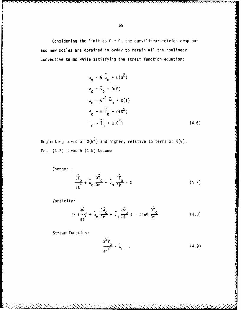
69
Considering the limit as G 0 0, the curvilinear metrics drop out
and new scales are obtained in order to retain all the nonlinear
convective terms while satisfying the stream function equation:
u - G u0 + O(G2)
v-v+ 0(G)0 0
wo 0~ G- w + 0()
f- G fo + 0(G2
T - T + 0(G2) (4.6)00
Neglecting terms of O(G 2 ) and higher, relative to terms of O(G),
Eqs. (4.3) through (4.5) become:
Energy:
;T 3T DT- + v - 0 (4.7)at
Vorticity:
0 0 ; w 0o (4.8)Pr {-- + u 0 + vo a (4
at
Stream Function:2-.
o = w (4.9)
.ro . 0

70
In these equations, the G dependency, which was again important in the
2-D N-S equations, has also vanished. The stream function equation
appears to be in boundary-layer format, as should also be the case for
the energy and vorticity equations when the viscous terms are included.
The inviscid (ore equations can satisfy the flow tangency condition,
but cannot satisfy the physical no-slip condition that must be met
at the walls, where the viscous terms play their important role. At
this point, one gathers from Eq. (4.8) that the gravitational terms
have reduced to simply sin 3T 0 /9r, as G - 0. This first-order term
is essential in driving the buoyancy-induced flow field, and its effect
seems just as significant in the adjacent boundary-layers, as will be
shown in the next section. Note, however, that the gravitational
term proportional to cosW 1T /31P comes in as a second-order
effect within the small-gap inviscid core solution. But its effect
should prove negligible (or of much less importance) within the
boundary-layers since being consistent with boundary-layer theory,
3T/3<< aT/ar.
4.2. The Boundary-Layer Expansion
To incorporate the higher order viscous derivatives, the inner
radial coordinate is stretched as
r-a rGa
where 5 is the inner boundary-layer thickness. Then, in it', tran, .,r"en

711
3f
state, the tangential velocity (v T- r) within the boundary-layer,
VBL' becomes (for a finite-gap size):
1 3f
VBL - 6 R (4.11)
and due to asymptotic matching principles, one must have
V Vc O(Ra 2) .(4.12)VBL vc
For this condition to hold, the stream function variable within the
boundary-layer must scale as
fBL 0(6 Ra /2 (4.13)
The raiial velocity (u - -+ ) then goes as f (for finite-gap),
or
uBL 0(6 RaI/2 (4.14)
From the definition of vorticity, one gets
VYBL )(Ra I ' (4.15)
A e' ' L _ 'r , i n trie core, it must also match
. " - . .'."., . " " us the boundary-layer
7. . . . . . . . . .

72
expansions are:
UBL = Ra1/2 U° +
VBL Ral/2 V0 +...
Ra/2WBL W +....
fBL 6 Ra l / 2 Fo +
TBL T + (4.16)
Using the above boundary-layer expansions together with the fact that
6 - 0 in the limit as Ra - , one can reduce the 2-D N-S equations to
the following form.
Energy:
Ra1/2 1 ;T oo+ VTo a __T
R a 0 * R a 4 - 2 2 -
Vorticity:
;W oo + o W Pr • a o
a t 0 a W S 2 Ra 1/2 R2
JT
+ sin R
Stream Function:
'2F a 2 W° (4.17)77 Wa
a"

73
and again, t : Ra 1 2t.
These equations clearly bring forth the scaling required for the
boundary-layer thickness, that is
R- 1/4- Ra-'1 (4.18)
where the 1/4 power is typical for natural convective laminar-type flows.
Using Eq. (4.18), the boundary-layer expansions become:
1/4 14UBL Ra U0 +
112VBL Ra V0 + 0()
W6L Ra 3/4 .+
(Ra1/ 4
f Ra /4F + 0(Ra 1 "4 )BL o
T = T + O(Ra - 1/2) (.19)TBL To
Physically these expansions make sense, since within the boundary-layer,
vorticity should be much larger than the stream function or velocity
components, and the tangential velocities should be greater than the
radial velocities for this particular flow geometry. Also, following
the same aforementioned steps, the outer boundary-layer thickness can
be shown to scale in the same manner as the inner one.
Now, as G 0 0, the boundary-layers must merge at some point
giving
" i m-- ' ""¢.. . "'" """" " "" """ ' " " " " . . . . . . . . . ....... . . . . I
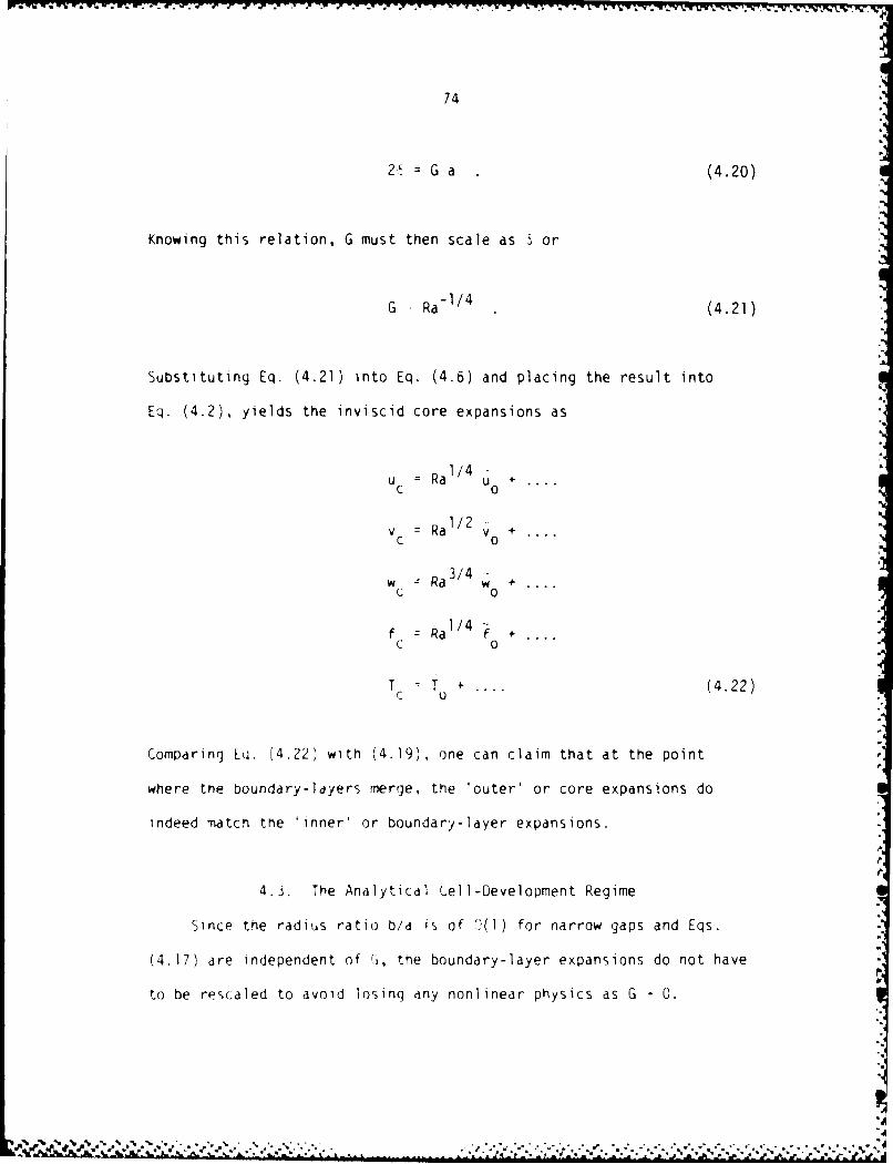
. q - .* ~~ *J. ~ ~ * W ~ - l ° -
74
2 G a (4.20)
Knowing this relation, G must then scale as 6 or
G Ra - I 4 (4.21)
Substituting Eq. (4.21) into Eq. (4.6) and placing the result into
Eq. (4.2), yields the inviscid core expansions as
u = Ra 4 uuC U0+
v = Ra 2 v +c o
w Ra3 w +c 0
f = Ra1/4 f +C 0
T r T .. . (4.22)
Comparing Eq. (4.22) with (4.19), one can claim that at the point
where the boundary-layers merge, the 'outer' or core expansions do
indeed match the 'inner' or boundary-layer expansions.
4.3. The Analytical Cell-Development Regime
Since the radius ratio b/a is of 0(l) for narrow gaps and Eqs.
(4.17) are independent of 1j, the boundary-layer expansions do not have
to be rescaled to avoid losing any nonlinear physics as G 0.
%

75
Therefore, it can now be inferred that the dependent variables in the
governing N-S equations will scale the same as in the boundary-layer
for the double limit of Ra - and G - 0. Thus, we take
G = Ra"1 /4 G (4.23)
and the expansions
u = RaI/4 u + O(Ra-1/4)
v = Ra1/2 v + 0(I)
3/4 1/4w = Ra3 4 w + O(Ra / )
f = Ra1/4 f + O(Ra-1 /4)
T = T + O(Ra - 2) . (4.24)
With Eqs. (4.23) and (4.24) in-hand, the 2-D N-S equations collapse into
Cartesian-like, boundary-layer type equations. In final form, they
become:
Energy:
-2 3T f @T f aT 1 2 (4.25a)G _+ G i _ a-- r- ---a i Pr (4.25a
9t Dr
I

w~~ ~ ~ V' W .; WJW T-; UV*Wj. -IW. n-rWIj x --. ~ ~ I 1i
76
Vorticity:
62 Pr-+G Pr{ fw + 2f aw
Pr a 2 + G sin * Dr (4.25b)
Stream Function:
2 G2 w (4.25c)
r2
with related boundary conditions of:
S(0,') : 1, T (1,') : 0 (4.25d)
(0,) : f (I,4) 0 (4.25e)
(0,4') GI r2 (4.25f)Tr r=O,l
where again, G, the scaled gap, is defined as
= Ra1/4 G (4.26a)
and the time-term is also scaled the same as in the boundary-layer, or
t Ra112 t (4.26b)
I~' V .V~~V .V ~V*..~ ~\f* J '~ I._
.1* ~ "

77
Equations (4.25) represent the key governing equations for arbitrary
Prandtl number in the double limit of Ra - and G - 0. The numerical
method used to solve these equations will be described in Chapter 5.
These equations can be further simplified under certain limiting
conditions. Three limiting cases will be investigated; namely, the
G - 0 limit, plus the vanishingly small and infinite Prandtl number
limits.
To leading-order, in the limit as G 0 0, Eqs. (4.25) reduce to:
Energy:
2i
Vorticity:
2-70
Stream Function:
S0 (4.27)
Thus, the energy equation simplifies to the steady-state 1-D
conduction equation, which integrates to
T 1 -r (4.28)
p, ,,., , -, ..- ,.,,, ,.,,-,, . , i ". ., ,- -,,,. .',,.. ', ", ,....,-.- .-. ,..,-. . ..... . ...-.. ..- -,,.,-.,

7 8
for the isothermal boundary conditions of this problem. Also, from
the no-slip condition, the vorticity and velocity components become
identically zero. Hence, convective effects are discarded, and the
temperature field becomes completely determined by the linear
relationship of Eq. (4.28).
From the above analysis, one can conclude that a Stokes-layer or
a conductive/viscous dominated flow field prevails as 0 C. Therefore,
the multicellular regime that is associated with the narrow type gaps
(at high Rayleigh number) most likely reverts back to two cells and
then, finally to a pure conductive mode when the velocities tend to
zero as G - 0 (or G - 0 for a specified Rayleigh number). Contrary to
this result, many investigators (Walton, 1980; Powe et al., 1971; Liu
et al., 1962) believed that as the gap approached zero, a true B6nard
type instability would evolve, where the typical critical Rayleigh
number (Ra b a ) of about 1,700 is approached. Instead, it appears that
after a certain point, the transitional Rayleigh number increases with
decreasing gap size (to well above 1,700), until eventually, a conduction-
dominated flow results as the gap approaches zero (see Chapter 6).
4.4. The Perturbative Solution to the Steady-State
Finite-Prandtl Number Equations
From numerical results obtained in this study, and results
discussed in Powe et al. (1971) and Rao et al. (1985), it can be seen
that the narrow-gap solutions for flows prior to multicellular
transition (and even beyond to a certain extent) behave in a

79
seemingly steady-state manner. Assuming the steady-state condition
and using the leading-order solution of Eq. (4.27), the convective terms
in the vorticity equation of (4.25) become zero. From this, w must
then scale as G in order to balance viscous and buoyancy effects, and
upon entering the stream function equation of (4.25), one sees that
f . This logic can be repeated in a successive manner (without
neglecting cross terms) until the following asymptotic expansions are
obtained for the steady-state case:
+ 14 16T = (l-r) + GT + GT 2 + GIT 3 + O(G1 )- +5 - 13w -1
w = G Gw +Gw + Gw 3 + + O(G )
- 3l 7f 11 lf + 15 + 9
=G3f+Gf2 +G f3 G 5f4 + O(G1 ) (4.29a)
while the related boundary conditions are:
T(O,W) = 1, T(l,f) 0 o
f(O') = f(l,,) = 0
r (0,) =- I (IP) = 0 (4.29b)
All of the important physics are included in the first two terms of
the expansions in Eq. (4.29a); that is, the gravitational, viscous and
convective effects are accounted for.
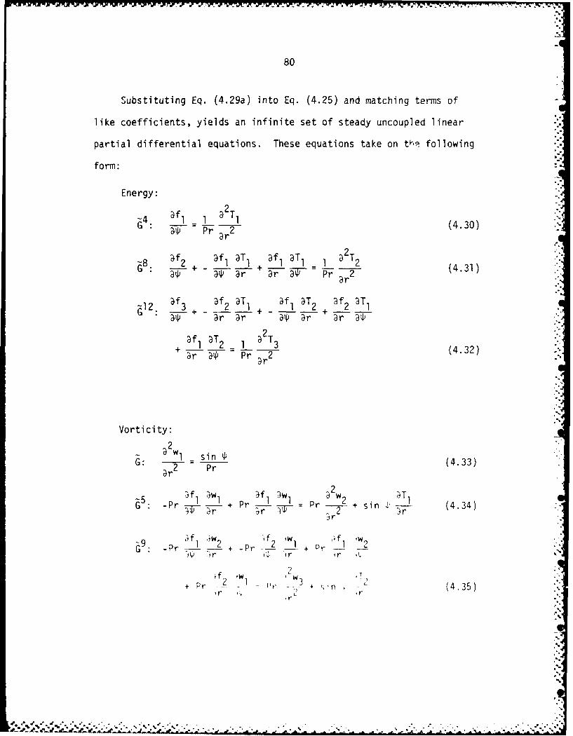
80
Substituting Eq. (4.29a) into Eq. (4.25) and matching terms of
like coefficients, yields an infinite set of steady uncoupled linear
partial differential equations. These equations take on tk- following
form:
Energy:
2-4 1 - 1 - T1 (430 -
Prr3r (4.31)
22
+ ±: 2 + 1 1 2T (4.32)
T r iP 3r 21 r r 9
22
Prf, 2 (4.33)
2 2
G: -r Pr (4.33)+
95 f w 4 f w
G -Pr + Pr-Pr-_ + s 1nPr . (4.34)92
Pr - r *. (4325)7
: d jl r. . r\~ 4. r ,-,

81
Stream Function:a2 fl
1 l (4.36)
2 2 w (4.37)
r2 2
3 3 w3 (4.38)
Equations (4.30) - (4.38) were solved analytically with the following
result (note: vorticity, temperature and stream function were carried
out to the first three nonzero terms):
(Al) (4.39)24 Pr
sin (Bl) (4.40)Wl T Pr
T cos (Cl) (4.41)1 44-0 (
96 Pr -P-(A2 + 9-) (4.42)
w sin 2* (C2+D) (4.43)2 96 Pr P
T2 cos 2 (E2 +2) + cos2(96 Pr Pr) 34560 (G2)
+ sin2L (H2) (4.44)
34560

82 I
f sin 2* cos (A B3) + cos 2* sin D 3
Pr --- ~-(C3+-2304 Pr 96 Pr P
96 Pr (3 Pr~ (G3) P
sin (H3)__ (4.45)34560.P
sin 2*cos* B4 cos 2* sin'P0
w3 2304 Pr2 Pr6 Pr P
+ cos 2*P sin E4* F4- + cos * sin *P (G496 Pr (E Pr~- 34560 Pr
+ sMn (4.46)34560 Pr (.6
where .
2 2Al =r (r-1) (4.47)
Bl r(r-l) + (4.48)
5 A 3
Cl =r(2r 5 6r 4 + 5r 3 1) (4.49)
and A2 through H4, which are also functions of r only, are given in
Appendix A.
In Equations (4.39) - (4.46), the stream function and vorticity
expansions have the same angular dependence, and to leading-order,
are inversely proportional to Prandtl number. For temperature, however,

83
the conductive term (1 - r) and Ti are completely independent of the
Prandtl number.
From Eq. (4.39), it can be seen that, to leading-order, the
stream function is positive for all i at a given value of r (for the half
annulus), and becomes zero at 0 = , T. Therefore, the primary basic
flow does indeed consist of two counter-rotating kidney-shaped cells
as discussed in the literature survey of Chapter 2. It is interesting
to note that the second and third terms of the stream function
expansion are proportional to sin 2*; thus, the basic flow has the
potential of obtaining more than two cells in the complete annulus -
especially when the Prandtl number is sufficiently small (Mack and
Bishop, 1968; Walton, 1980).
Before completing this section, the asymptotic expansions of
Eq. (4.29) will be placed in a compact recursive notation:
(1- r) + z G4n T
n=l n
I 4n-3
n=l n
f 4n- l f (4.50)n=1 n
The angular dependent coefficients (to be denoted by F, W and T) in
Eqs. (4.39) (4.46) can also be written in the following revealing
notation:
I
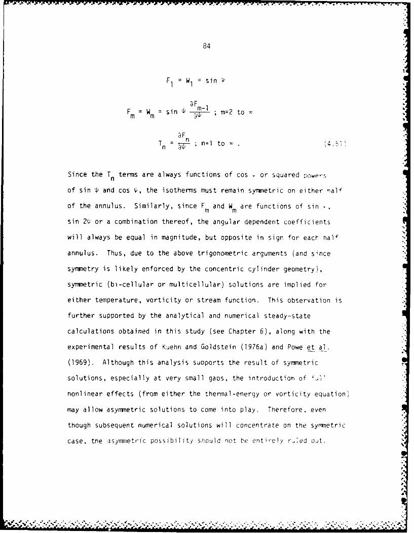
84
F1 1 = sin '
Fm Wm sin , m-2 to
3Fn .
Tn n ; n=l to . (4.51
Since the Tn terms are always functions of cos or squared powers
of sin and cos W, the isotherms must remain symmetric on either nalf
of the annulus. Similarly, since F and W are functions of sinm m
sin 2y or a combination thereof, the angular dependent coefficients
will always be equal in magnitude, but opposite in sign for each half
annulus. Thus, due to the above trigonometric arguments (and since
symmetry is likely enforced by the concentric cylinder geometry),
symmetric (bi-cellular or multicellular) solutions are implied for
either temperature, vorticity or stream function. This observation is
further supported by the analytical and numerical steady-state
calculations obtained in this study (see Chapter 6), along with the
experimental results of Kuehn and Goldstein (1976a) and Powe et al.
(1969). Although this analysis supports the result of symmetric
solutions, especially at very small gaps, the introduction of f61
nonlinear effects (from either the thermal-energy or vorticity equation)
may allow asymmetric solutions to come into play. Therefore, even
though subsequent numerical solutions will concentrate on the symmetric
case, the asyrrnetric possibility should not be entirely rxfled out.
LZ.
a
._'W' , % , .. -,,%-. -. % -............................-.......-.............-.-..-..-..... ... ......-..
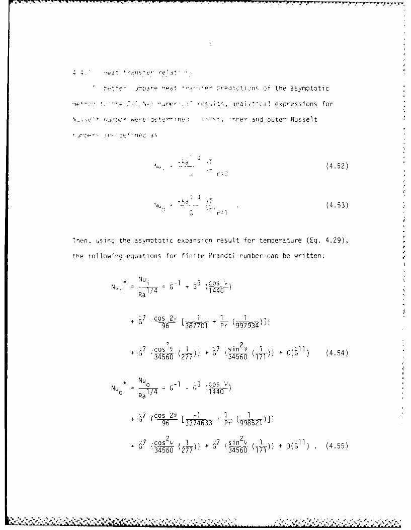
.~~~r . . .ela! F-~
,**, .m~r-e iea! *i, ~: ~ i )n s of the asymptotic
I *"e .i- - ner, -es~ ts, anal tica I expressions for
rr e we~e e lli.rS*~ ner 3fld outer Nusselt
A -- a(4.52)
i - (4.53)
Then, using the asymototic expansion result for temperature (Eq. 4.29),
th~e Tollowinq equations for finite Prandtl number can be written:
Nu GRa /41440
+ 97 6 387701 +r 9 97934)]
2G a7 ~-o' 7 -sin 0 1454~34560 T277~ G 34560 171~- (G 1 (.4
Nu Nu 0 G-1 G ~3 (COS
+ a7 cos 214 [ 1 +
+ 3S6 G ~ 7) G I36 )) + 0( G ).(4.55)

-R166 113 THE NUMERICAL RND RNALYTICRI. STUDY OF BIFURCATION AID 2/3MULTICEU.ULAR FLO.. (U) RJR FORCE INST OF TECHNRIGHT-PSTTERSON SF9 ON 0 FANT 196?
UNCLSSIFIED FIT/C/NR-13 F/ 29/13 L
mhhhhmmhhhmhmlsmhhhhhhmmsm

-7 RU1
T NEF.F] :11.2.
111I 2 Ijll 1-4 11111-
k -
*W
p.
, I .'::z- " " +' : :, ', ' ; P ' '," -'- 4 " '"" " , - ." I--,- IH--' . '. "-p ". - - "" - - ''.+"-"",," ," " """

86
The first term in Eqs. (4.54) and (4.55), G-, represents the purelyconductive contribution to heat transfer. The convective influence
is provided by the remaining two terms of order 6' and 7.
In the limits as Pr - 0 and Pr - - (see Sections 4.5 and 4.7),
analytical expressions for the inner and outer Nusselt numbers can
also be obtained. Hence, from forthcoming equations (4.76) and
(4.106), one gets:
For Pr - 0:* *
Nui = Nuo = G-I (4.56)
where G is given by Eq. (4.67), or
G G Pr-I 4
For Pr
N* 6--1 + G3 (cosP + 7 cos 24 1Nui : G- + G31440- + 96 (387701}
+ 7COS2 ( _L)} + 67 sin' (1-)}34560 277 34560 17
+ O(Gll ) (4.57)
Nu* - 3 (cos' + G7 {cos 21 -10 1440 96 (3374633)}
+ 67 cos21 1 + 67 (sin __} + 0(11
+ 34560 + 34560 )
(4.58)

87
Equation (4.56) signifies the pure conduction result for Pr 0 0, and
thus, does not retain any convective influence to heat transfer.
Equations (4.57) and (4.58) are similar to those for finite Prandtl
number, except terms proportional to Pr-l have vanished.
4.5. The Zero Prandtl Number Limit
In this section, the previously derived small-gap (finite-Prandtl
number) equations will be used to analyze the theoretical effects as
Pr - 0. From a practical standpoint, the behavior of liquid metals should
fall within this low-Prandtl number approximation, and this analysis has
application to the study of liquid metal-cooled nuclear reactors.
It appears from the literature that Pr - 0 limits have not been studied
either numerically, analytically or experimentally for the horizontal
narrow-gap concentric cylinder geometry. Lee and Korpela (1983) have
studied a similar type of natural convective flow between vertical
slots, where the left wall is heated. They demonstrated that in the
narrow (high aspect-ratio) slots, a stationary multicellular flow
resembling an hour-glass configuration is initiated near the center
of the slot, and appears strongest for the near-zero Prandtl number
cases. But the source of this unique instability is hydrodynamic
rather than thermal, because for Pr - 0, the large thermal diffusitives
that result most probably rule out any type of thermal perturbations.
Realizing this, one can speculate that in the vertical portions of a
narrow horizontal annulus, the same type of hour-glass shaped
hydrodynamic instability is possible. Furthermore, Korpela (1974) and

MMIN 171 Ti 17 IT -~ KV 7V-I- -Z -T
88
Walton (1980) discuss the fact (for flow due to natural convection in
an inclined channel, see Chapter 2) that for Pr > .24, a true Benard-
type thermal instability prevails, whereas for 0 < Pr < .24, a mixture of
thermal and hydrodynamic instabilities result, until finally at Pr = 0,
the instability is purely hydrodynamic. Thus, one might now look upon
the narrow horizontal annulus geometry as a combination of horizontal,
inclined and vertical channels. Both types of instability appear to
have a definite role in the cellular patterns that develop in this
geometry, as a function of Prandtl number. Therefore, the small-gap/
finite-Prandtl number equations derived in Eq. (4.25) may prove useful
in studying the cellular-structure variation with Prandtl number.
But, since the limiting equations for Pr - 0 have not yet been obtained,
the following analytical analysis was conducted.
To begin, let Pr 0 0, and assume again that temperature is of '.
0(l) from the boundary conditions. Then, assume that
w =X 1 W +.... (4.59)
f X2 F ... (4.60)
and consider the stream function equation in (4.25) to get
X 2 ~ 2 X 1 (4.61)
Using Eqs. (4.59) and (4.60), the vorticity equation in (4.25) becomes:
.5'
;.
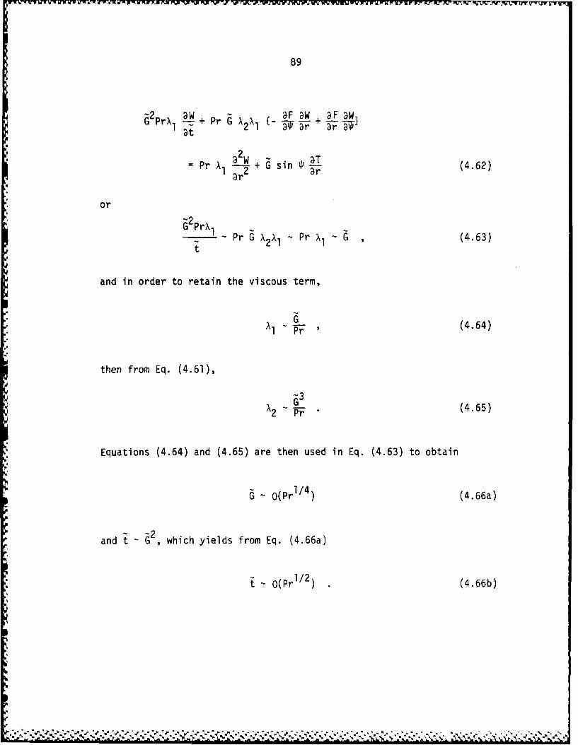
89
G2 PrX 2- + Pr G Xa F 3W 3F 9W1 at 2 ~ 4 1 TT + Tr-3
=Pr X1 a W + si 'T (4.62)
or
Pr G X2x I - Pr X1 - G ,(4.63)
t
and in order to retain the viscous term,
xl - 6 (4.64)
then from Eq. (4.61),
X2Pr (4.65)
Equations (4.64) and (4.65) are then used in Eq. (4.63) to obtain
G-O(Pr 1 4) (4.66a)
and t- G , which yields from Eq. (4.66a)
t-O(Pr 1/2) (4.66b)
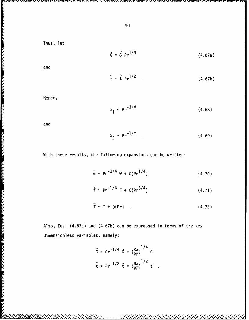
%-Lvw-~ ~ ~ ~ ~ %mFl . jWLAIrLW-~VF~W7VwVwIjWT.'.T' 4 Q rYY~rrT. ~r~'LFVV~V.WV in"
90
Thus, let
G = G Pr11 (4.67a)
and
t= t Pr~' (4.67b)
Hence,
X -3/ (4.68)
and
X2 Pr11 (4.69)
With these results, the following expansions can be written:
- -3/4 1/4 (.0
w - Pr W + 0(Pr )(.0
f- Pr-1/4 F + 0(Pr3/) (4.71)
T -T +(Pr) .(4.72)
Also, Eqs. (4.67a) and (4.67b) can be expressed in terms of the key
dimensionless variables, namely:
G Pr-' P ra) 1/
1/2 (~1/2 t

U 91
These new scales, when written in the above form, clearly display
their unique dependency on Ra, Pr, G and t. Upon substituting Eqs.
(4.70), (4.71) and (4.72), Eqs. (4.25) reduce to the following set
in the limit as Pr - 0:
Energy:~2TT= 0 (4.73)
'U' Vorticity:
'2 3W 3F 3W +F 3W a G n Tt _ + G { + G sin aT (4.74)at 3TT r2T r2 3r
Stream Function:
a 2F - a2 W (4.75)3r
2
The energy equation in this case also reduces to the steady-state
conduction equation. For the boundary conditions considered, the
linear temperature distribution across the gap takes on the following
simple solution:
T = l - r (4.76)
Thus, as Pr - 0, only concentric isotherms should result, regardless
of the flow field that develops. The energy equation has now
completely uncoupled itself from the vorticity equation, and since
..
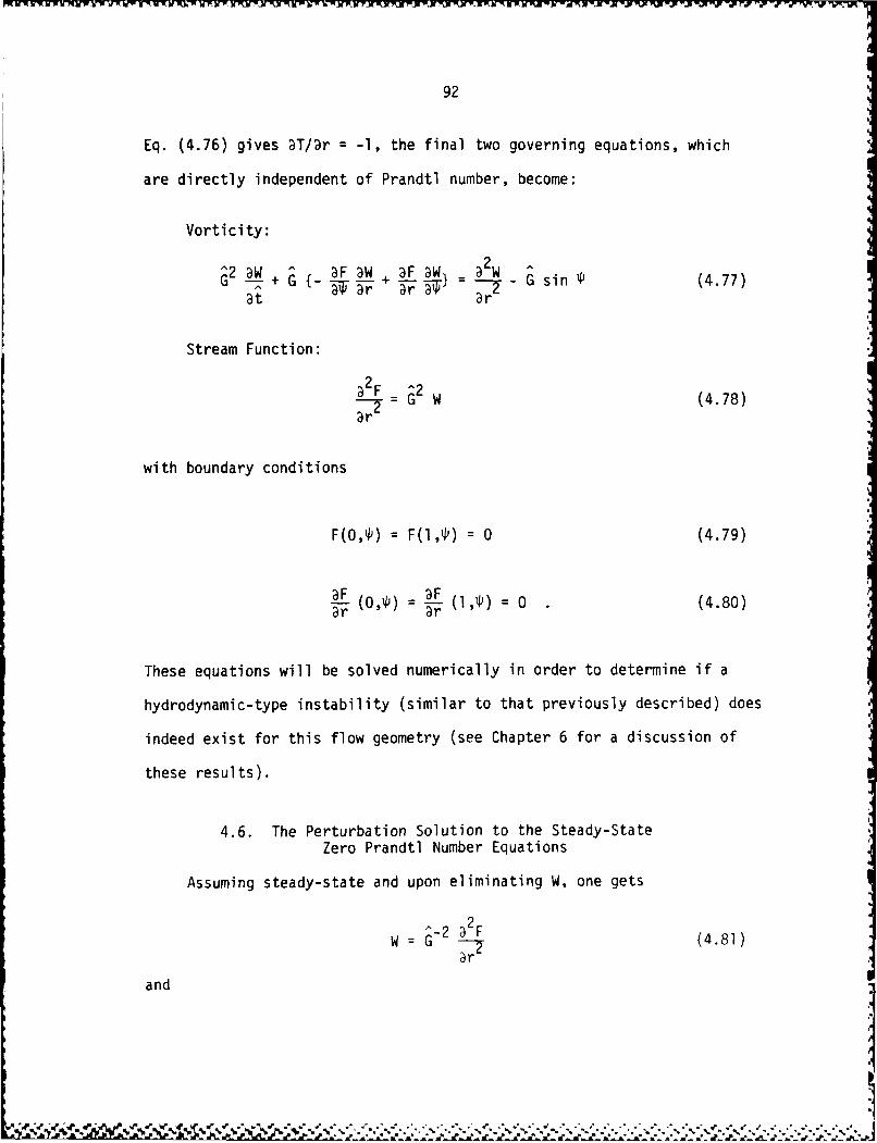
92
Eq. (4.76) gives aT/Dr = -1, the final two governing equations, which
are directly independent of Prandtl number, become:
Vorticity:
^2 3W 3F 3W + F 3W a 2 WG2 _ + G {_ W T -- G sin (4.77)
at 3r
Stream Function:
"2F 62 W (4.78)
with boundary conditions
F(O,f) = F(l,l) = 0 (4.79)
F (OM = F (lW) =0 (4.80)
These equations will be solved numerically in order to determine if a
hydrodynamic-type instability (similar to that previously described) does
indeed exist for this flow geometry (see Chapter 6 for a discussion of
these results).
4.6. The Perturbation Solution to the Steady-StateZero Prandtl Number Equations
Assuming steady-state and upon eliminating W, one gets
W G 2 F (4.81)3r
and
:1

aY TOT
93
3F a F _ 3_F_ 4 F 63
G 1- W T r 2 sin . (4.82)I ar arThe logic used to derive the expansions in Eq. (4.29) when G - 0 can
again be used to derive the expansions for the G - 0 limit. Thus,
considering Eq. (4.82), the stream function expansion should behave as
31 + l 15FOG(F GF 2 + F3 +( ) (4.83)
and from Eq. (4.78), the vorticity expansion becomes
W G W + GW2 + G W 3 + 0(G) (4.84)
Notice that the power of the coefficients in the above expansions is
identical with those in Eqs. (4.29), as should be the case. However,
in deriving the asymptotic expansions of Eqs. (4.29), the buoyancy
aTterm, G sin ' -T (in Eq. 4.25b), maintained the same order as theIDr
viscous term for all orders of the vorticity expansion. But for the
Pr - 0 limit, the buoyancy term comes directly into play only in the
leading order W term, where the viscous term is balanced by the
buoyancy force; while in the other terms of the vorticity expansion,
the convective forces are equated with the viscous ones and the
buoyancy effects contribute only indirectly through F1 and WI.
Substituting expansion (4.83) into Eq. (4.82), and matching terms
of like coefficients, yields the following steady-state result:

94
G r--4- sin 4 (4.85)
^ 7 a 4 F2_ 3F 13 FI + Fl a 3FI1
G 4 T F r3 3 r rTF (4.86)
Integrating Eq. (4.85), one gets
_ r4 r3 r2F, sin + c L+ c2 + c r + c , (4.87)
14 3. 2 3 4
while the constants of integration are obtained from the boundary
conditions of Eqs. (4.79) and (4.80) to give:
F = r2 (r-1)2 sin (414 (4.88)
Differentiating Eq. (4.88) twice with respect to r gives
W = {r(r-l) + 1} 4 (4.89)6 2
Using Eq. (4.88), Eq. (4.86) becomes
4F 2 = {6r 5 - 15 r4 + 14 r3 _ 6 r2 + r} 2 sin N (4.90)ar4 242
Integrating Eq. (4.90) and applying boundary conditions (Eq. 4.79) and
(Eq. 4.80) yields
..

95
F = sin 24'2 96 (B2) (4.91)
and W2 follows as
sin 2(2 96 (02) (4.92)
where B2 and D2 are the same as those in Eqs. (4.42) and (4.43), and
again, are given in Appendix A.
The equations for F1 , W1 and F2 , W2 take on forms similar to those
in Eqs. (4.39) through (4.43), except that in the former, the Prandtl
number dependency and the coefficients A2 and C2 completely vanish for
the limit of Pr - 0. Then, by neglecting terms A3, C3, E3 in Eq. (4.45)
and A4, C4, E4 in Eq. (4.46) for the limit as Pr 0 0, one easily
obtains solutions for F3 and W3, respectively.
Since F2, F3 and W2 , W3 involve terms proportional to sin 24, it
can be reasoned that these terms must contribute to the potential
multicellular transition of the flow field occurring at some critical
value of G. By performing a simple order-of-magnitude analysis, one
can estimate when these terms become of equal importance with the
leading order expansion terms. From this result, the onset of
multicellular flow can be approximately predicted. Carrying out this
analysis, one finds that the sum of G7 F2 and GI F3 achieves the same
order as G F1, when G = 7.2. Similarly, for vorticity, G 2 and OW3
achieve the same order as GWl at G = 7.5. Hence, the critical value
of G appears to be about 7.

96
For the pretransitional cases, the first-order expansions of
Eqs. (4.83) and (4.84) provide good approximations in describing the
behavior of stream function and vorticity (respectively) for the limit
as Pr - 0. Since it is likely that terms beyond F3 and W3 play
dominating roles in triggering the instability, the critical value of
G might be lower than that predicted by the above order-of-magnitude
analysis. To properly estimate this value, the full effects of
nonlinearity must be taken into account. This will be done in Chapter 6
when the equations are solved numerically. Considering the above
discussion, one obtains the following relations:
F 2 2 sin 'PF G r (r-1) 24 (4. 3)
W 1 sin 'PG {r (r-l) + } s2 (4.94)
Equations (4.93) and (4.94) represent analytical profiles for the
steady-state pretransitional stream function and vorticity, which
are valid throughout the annulus (0 - 2T). Comparisons to related
numerical results will be given in Chapter 6. From these relations,
it can be seen (for the half-annulus) that the vorticity given by
Eq. (4.94) takes on positive values within the boundary-layers (for
r near zero and one), and negative values within the inviscid core.
The stream function (from Eq. 4.93) always remains non-negative, since
the r terms are squared. This reasoning can be extended throughout the
entire flow field, at least for the bicellular case.

97
Referring to Eqs. (4.93) and (4.94), it can be seen that any
resulting bicellular profiles must be symmetric with respect to both
the vertical and horizontal centerlines, or at O=, T, T and L2r2' 2 n .Ti
suggests that for the Pr - 0 limit, the pretransitional flow fields
are completely symmetric, although the possibility exists for the
occurrence of asymmetric solutions due to nonlinearity, especially
after the onset of instability. In addition, for the half-annulus
basic cell-structure, the stream function achieves its maximum, and
vorticity its maximum or minimum (depending on r), at P = j for any
particular r location.
Furthermore, because the extremum stream function location
occurs at (or very near) T2 2j r for Pr - 0, and since the buoyancy
term sin ip reduces to -sin i for this case, one can speculate that@r
the upward or downward shift in the stream function's position (caused
by an increase in Rayleigh number) is probably dependent upon theT
magnitude of L-and the type of fluid used - or the value of Prandtl
number.
4.7. The Infinite Prandtl Number Limit
To properly complete the analytical analysis of this particular
flow geometry, the other end of the Prandtl number spectrum will be
considered. Thus, simplified governing equations are sought for the
Pr - ' limit. Many important fluids (such as glycerin and most oils)
possess a large Prandtl number dnd should be fairly accurately described
by the infinite Prandtl number approximation.
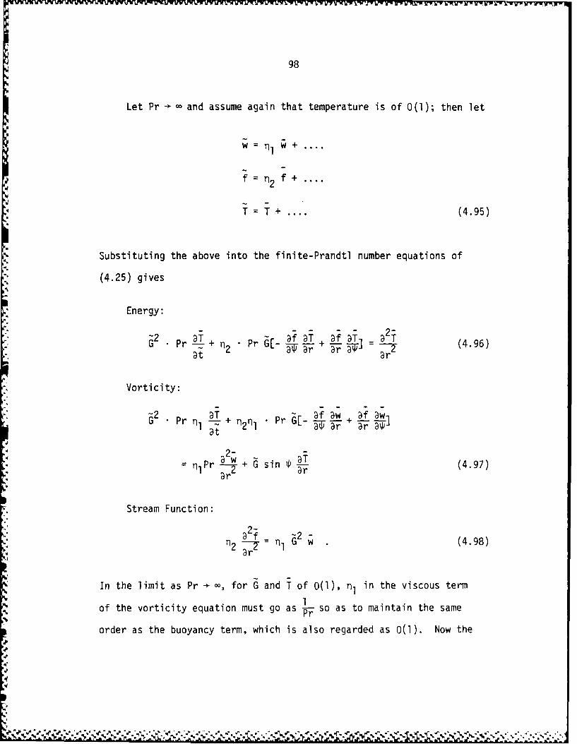
98
Let Pr o and assume again that temperature is of 0(1); then let
=n2 f+....
T + .... (4.95)
Substituting the above into the finite-Prandtl number equations of
(4.25) gives
Energy:
G 2 . Pr- afDT f D a Tr n2 r r -- 7 (4.96)
Vorticity:
'2 Pr TI T + n2nl Pr af aw + f awat
: -Pr a + G sin 9- (4.97)
3r a
Stream Function:
2-
rn2 a f TI w (4.98)
In the limit as Pr 0, for G and T of 0(1), n, in the viscous term
of the vorticity equation must go as 1- so as to maintain the same
order as the buoyancy term, which is also regarded as 0(I). Now the
;61

nil X7 TA . - . W V W .
99
stream function equation must be satisfied; thus from Eq. (4.98), one
obtains
1n2 -~ l Pr ~p(4.99)
and this expression for n2 also satisfies the energy equation of (4.96)
at steady-state. However, the unsteady time term in the energy equation
can be retained by scaling t as
t = Pr t (4.100)
or from Eq. (4.26b) one gets
- .i1a/ 2
Pr = ( pr )t (4.101)
Hence, for the Pr limit, the following expansions result:
w = Pr 1 w + O(Pr 2)
= Pr 1 f + O(Pr -2)
T = T + O(Pr - ) (4.102)
With Eqs (4.100) and (4.102) in-hand, the governing equations become
(in the limit as Pr c):
I

100 ',
Energy:
- - - - - 2-3T f T + f 3T D Tt + - --3T3 (4.103)
Vorticity:
a2w IT
+ G sin 3r-0 (4.104)
Stream Function:
a 2i _ 2 w (4.105a)
ar2
with boundary conditions
T(O'P) = , T-(lP): 0
f(o,') = f(l, ) 0
and -- (0,) _ - (1,') = 0 (4.105b)
By letting Pr 0, the nonlinear convective terms in the vorticity
equation have completely dropped out. However, since the nonlinear
terms in the energy equation still remain, the decoupling effect
between the energy and vorticity equations is no longer possible, as
it was with the Pr - 0 limiting solution. Also in the above equations,
the Prandtl number dependency has again been eliminated.
A!
pN

101
Similar to the finite-Prandtl number equations, the G - 0 limit
yields a purely conductive-dominated flow field, where again, the
temperature profile reduces to the 1-D steady-state conduction case.
Hence, steady-state expansions can once again be found by proceeding
with the G -~ 0 solution. As expected, the expansions that result take
on the same form as those in Eq. (4.29a):
T= (l-r) + 64 T + 68 T2 + 0(G12 )
w= Gw1+ 0w 2 + 0(69)
f =3 fI + 67 f2 + 0(G11) (4.106)
Perturbative solutions to the infinite Prandtl number equations are
readily found by neglecting the Prandtl number dependency and the
coefficients of o(L) relative to those of 0(l), in Eqs. (4.39) throughPr
(4.46). This approach is similar to that used in the Pr - 0 limit,
but with opposite terms neglected.
Finally, then, in the limits of small and very large Prandtl
number, the governing equations for the narrow-gap limit have become
much simpler. In the former, the nonlinear terms in the vorticity
equation (which could give rise to hydrodynamic instabilities) dominate,
whereas in the latter case, the nonlinear terms in the energy equation
(which should give rise to thermal-type instabilities) dominate. Thus,
by examining these two limiting conditions, the crucial mechanism for
causing potential natural convective instabilities between narrow
N N N

102
concentric horizontal isothermal cylinders is clearly set forth.
Simplified governing equations for Pr - 0 and Pr - - can also be
obtained from the 2-D N-S equations, which include both buoyancy
terms and are valid for arbitrary gap size and Rayleigh number. These
limiting conditions are explored and discussed in Appendix B.
Although the material in this chapter is very analytical in nature,
many of the equations derived (with the exception of those relating to
the infinite Prandtl number limit) will also be solved numerically in
Chapter 6. Hence, useful comparisons to the analytical results can
be made, and the critical effects of the nonlinear terms can be
interpreted.
4
103
5. NUMERICAL ANALYSIS
This chapter is divided into two sections. The first describes
the finite-differencing method used in solving the coupled set of
governing partial differential equations. Two systems of equations
will be considered: the 2-D unsteady elliptic Navier-Stokes equations
derived in Chapter 3, and the 2-D unsteady boundary-layer equations
developed in Chapter 4. The second section deals mainly with
describing the numerical procedure employed in determining the onset
of an instability, either thermal or hydrodynamic, for both the 2-D
Navier-Stokes and boundary-layer equations. Procedures for capturing
related hysteresis behavior will also be discussed. In addition,
important computational details will be provided at the end of this
section.
The essential features of the numerical method were adopted from
Prusa (1983). However, several important modifications were
incorporated into his scheme in order to enhance numerical stability
and efficiency when solving the system of equations in the high Rayleigh
number/small-gap multicellular flow regime. Of particular importance
was the handling of the nonlinear convective terms, in which two types
of representations were employed: a corrected second-order central
difference scheme for the 2-D Navier-Stokes equations, and a
corrected second-order upwind scheme for the boundary-layer-like
equations. Also, the unsteady form of the equations was used to take
advantage of achieving steady-state in a more stable manner and

104
allowing the opportunity to capture unsteady behavior when solved in
a time-accurate fashion.
5.1. The Numerical Method of Solution
The 2-D Navier-Stokes equations outlined in Eq. (3.1) are
discretized using finite-differencing techniques. This converts the
equations into an algebraic system that is well-suited for computation
on a high-speed computer. In the transformed plane, the computational
domain was divided into a number of cells. This cellular mesh was
formed by the intersection of a set of radial lines with a set of
circular arcs concentric with the boundary, r = 1. The grid nodes are
variably spaced and are defined by the intersection of these radial
lines and concentric arcs. The variable increment nodes are depicted
in Figure 5.1 by using an extended version of Southwell's (1946)
notation in the immediate neighborhood of a typical node. Initially,
the complete annular flow field (0 to 2f) was resolved numerically.
However, if symmetric cellular patterns resulted, vertical symmetry was
assumed and only the half-annulus (0 - Tr) was computed for
subsequent calculations.
The use of variable increments allowed for the concentration of
grid nodes in areas of large gradients within the computational
domain, such as the inner and outer boundary-laye-rs and the thermal
plume region near the top of the inner cylinder. iowever, it should
be noted that the use of variable increments may result in a loss of
formal truncation error (Roache, 1976), where the loss becomes less

.105
5'.j
1C~I
c.4)
co.
C~£
% %
106
severe in the finer portions of the mesh and more severe in the coarser
areas (this result is discussed further in subsection 5.1.2). A
convenient 2-D coordinate variable mesh routine was developed in
Prusa (1983), in which the variable nodal positions were computed by
using a smooth fourth-order polynomial stretch that imposed a zero
gradient increment variation at the edges of the mesh. This routine,
with minor changes to accommodate the complete (0 - 2Tr) annulus, was
used in this study to generate the various computational meshes. The
program was relatively simple to use and proved quite valuable in
resolving the multicellular flow field.
5.1.1. Variable increment finite-difference formulas
The formal Taylor series approach will be used to develop variable
increment finite-difference approximations of the derivatives in the
governing equations. The dependent variables T, w and f will be
denoted by ¢; kf and kb denote the increments in the directions of
increasing and decreasing angular variation, from a given discrete
point (ri, 4'.) (see Figure 5.1). Using Southwell's notation, the
Taylor series expansions of 2 and 4 (ri,'.) are:
+ k + k 2+ 1 kf3 + (5.1a)2 = 0 kf + 2 k...2 0 0 2~'of 6 t~
'o b 2 1 3 kb3 + ... (5.1b)4~ = 3z b 2 0 k b2 6 3 0 k b 3
L4 ¢F: ' . " . . . . . . . . . . - . . . . . .

107
Equation (5.1a) can now be solved explicitly to give a forward-
difference representation of / :
kf1 + 0(kf) ,(5.1c)
while Eq. (5.1b) yields the backward-difference form:
0 O + O(kb (5.1d)
Subtraction of Eq. (5.1b) from Eq. (5.1a) gives the (second-order-like)
centered-di fference result:
0 2 kf + +O(kf - kb + 0(kf2. kfkb kb 2 (5.1e)
A second linear combination of Eqs. (5.1a) and (5.1b) gives the
centered second derivative:
a2 k -0 k + k00+kf0
(kf 2b10 (kkf4k~-(f + b)kfk b
+ O~k f - k b) + 2~ k f kb' k b) (5.1f)
The counterpart radial expressions for Eqs. (5.1c) through (5.1f)
are easily obtained by substituting r for iand cO1, 43 and hf, h b for
108
¢2' c4 and kf, kb, respectively.
Finite-difference formulas for the unsteady terms are found by
using the standard, but generally stable, forward-difference molecule:
n+l n_ 0 - 0 + O(At) (5.2)
at 0 At
where n designates the time level at which the dependent variable $ is
evaluated. When marching in time to steady-state, the first-order
truncation error should not influence the final result; hence, time
steps as large as possible should be considered. However, when
unsteady behavior had to be resolved (as with the Pr - 0 case in this
study), very small time steps should be used to avoid large truncation
error, thus obtaining a time-accurate solution.
5.1.2. Finite-difference equations for the dependent variables
All spatial derivatives in the governing equations are second-order
centrally (or upwind) differenced. This includes the convective terms
which are represented by a first-order upwind expression together with
a correction term for second-order-like accuracy. The convective terms
are split in order to maintain diagonal dominance of the coefficient
matrix at high Rayleigh numbers (as with pure upwind differencing),
thus providing stable convergence toward the desired centrally
differenced (or second-order upwind differenced) representation.
5.1.2.1. 2-D Navier-Stokes equations The nonlinear convective
terms in the 2-D Navier-Stokes equations can be expressed as:
II

109
2 t- 3 +p 1 + H03 - (1 + H)O02 r = ( - IXI) { h + hb + hf
-l -(1 ++0 -+ 3 (5.a
+ + jj) {l hf hb + hf (5.3a)
and
2p an -@ 4 +2 + k 4 - (I + k)o 0U 0 k kff+ k b
+ N + 0- 0 02 + 04 "k(I+(5kb k f +kb+ H + I ) {____ 2f kf +k kb } (5.3b)
where 0 represents the dependent variables T, w, or f, and
_ h k
The first terms within the brackets are the first-order upwind-difference components and the second terms are the added corrections
which bring the differencing up to second-order accuracy. The terms
within the parentheses (outside of the brackets) ensure that stable
differencing 'into-the-wind' is enforced.
Using the above relations, Eqs. (3.1a, b, or c) can be manipulated
into the following general form:
2 -)2 2A2 {- AG2 t + (r + a) + 2A Xr+ 2 - + S 0 (5.4)
3r G lp2
;
S

110
where
2A (r + -) {A2 + Al 3f} (5.5a)
2p (5.5b)r +
and
Pr, ¢ T 1, :T
Al : Pr, w A2= Pr, p=w
0, ¢=f 1, t=f
while
Pr, = T
A Il, w
0, ¢: f
The derivatives in Eqs. (5.5a) and (5.5b) are represented by standard
central-difference expressions, as in Eq. (5.1e).
Employing Eqs. (5.3a and 5.3b) and substituting the appropriate
differences of Eqs. (5.lc-f), results in a general finite-difference
equation for ¢ = T, w, or f:
= A n0 + CI Cn+l
+ C3 3n+l + C44n+l + En + Sn+l (5.6a)
+Cp Cr E +A
where
C (A2) A G + 2[hA2 + A2
fb kf kb (r + 1
+ xL L + X ! +!w-) +F r (hf hb hb hf kf kb
+ Fr11 (1 + 1L-.6b
= 2(A2) + (x + lXI) (.cC1 hf hf + hb) h f (.
C22 (A2) + r' + PLi) (5.6d)(r + I ) 2(kf + kb)kf kf
03 = 2(A2) ( x (b.6e)
C=2(A2) FW- 411)4 (r + 2. (kf +k)kb k (5.6f)
* Note that a negative contribution to C~ is possible if hf/hb or kf/kb
departs too far from 1. Thus, unstable calculations may result if
diagonal dominance is lost as Co gets smaller in magnitude.

112
En ___{___ ( I n3
h h ,n (1 + n (H - 1) - n (H -hf + hb 1 H 30 H
I xJI) nf (l + .1) + n ( (2 + H +1(hf + hb I3 (1 + H) - (0
(f+k n 1l- n n 1)
+ r bp_) {,n (1 4) + ,n (k - 1)- n0 (k - -1
kf +kb 2 K 40 k
r , n (I + _L + ,2 n n+1} (.g"(kf + kb 2k 4 (l + k) - (2+k+(.g
0 T
F n+lSn+l G Ra (sin T + cos aT W
0 r + 10
-G 2 w 0n+ l , = f (5.6h)
and I, = T
1, =w
0, p : f (5.6i)
The derivatives - and - in Eq. (5.6h) are evaluated by usingar e0 f u dt
standard central-difference formulas. T denotes the time increment,
T*-.--- Kr IV K"A-m . -K -A
113
while the superscripts, n, n+l, are as discussed in Eq. (5.2).
For a fully-implicit method, the correction term E, should be
evaluated at the new-time level, E .+l However, as seen in Eq. (5.6g),
the correction term for the 2-D Navier-Stokes equations was evaluated
at the old-time level, En. Although the En method introduced a time
truncation error of O(At), it still remained consistent with the rest
of the formulation. Also, since En uses known information from the
previous time level, its contribution to the off-diagonal terms (,
n2' 3 nand 04) was kept constant when evaluating flow properties at
the new-time level. This factor apparently helped to enhance
numerical stability, which in turn, improved the convergence rate and
accuracy of the numerical method when compared to the En+l
formulation. This was especially true for the highly convective flows
associated with multicellular development (see Appendix C). In comparing
n+l nto En , a truncation error analysis demonstrated that the E method
preserved the formal accuracy of the system of equations. A
description of this analysis and a tabular comparison of the two
approaches is given in Appendix C.
5.1.2.2. Finite-Prandtl number boundary-layer equations The
boundary-layer equations of (4.25) are numerically treated in a manner
similar to that used on the 2-D Navier-Stokes equations. But since
Eqs. (4.25a-c) are only first-order in >,', a slightly modified version of
Eq. (5.4) results:
A2 {-A G2 2w4 1 + 2X + 2u =(5.7)Dt 3r Or

114
where
2X = Al a (5.8a)
2 p = A - 3 (5 .8 b )Dr
The first-order derivatives in the 2pj and 2X coefficients are
approximated by central-differences. Also,
Pr G, do T 1, =-
Al = Pr A2 Pr, w_
0, 1O = , = "
while
( Pr, = T-I-
Aj 1, d=wo,
Except for the definition of X, the convective term 2A - is
represented as in Eq. (5.3a). However, because of the parabolic nature
of these boundary-layer equations, which are first-order in lP, a central-
difference representation of the streamwise convective terms is no
longer valid. Instead, a stable corrected second-order upwind-
differenced scheme is employed. Namely,

-u jw -j Jr ~n ~r. r
115
kbc* 0 " ¢4 + k- l ) 1 0 - 4
2ii = (i- I I) { 0kb4 +kb ba0 k kb + kb1
kf.
2 - ¢ + ( -kfi)( 2 - 12 )
+ N + IIl{2k0+ kf + (5.9)
kf kf +k f 1
(see Figure 5.1 for related nodal positions). The second term within
the brackets represents the added correction to the first-order
differenced component needed to achieve a second-order upwind-
differenced expression.
Using the above results, the boundary-layer equations of (4.25)
can be cast into a finite-difference form similar to that of Eq. (5.6a):
C0n+1 (A2) 2 n + n+l++ l
C o ¢o + Cl l + C2 2 n+l + C3n + l
+ C404n+l + En+l + Sn+l (5.10a)
where
C (A2)A 2 + 2 (A2) + rA( 1 + + 1: h hf hb h f h hb) + h b + ff
Lr() + (I- + 1-) (5.10b)kf kb kb kf

116
C 2 (A2) + r(x + XIl (5.IOc)I h f(hf + hfb hf
C2 = r(u + Jl) (5.1Od)kf
C3 2(A2) r(X- (5.1Oe)3 (hf + hb)hb hb
-r= - I ) (5.1Of)C4 k kb
and r is defined as in Eq. (5.6i), with 4 now denoting the boundary-
layer dependent variables. Before defining the correction term En+l
let
kl I k2 = cb' d
where a = kf, b = kfl, c = kb, d = kbl. Then:
E n+l 1,n+l l n+l (H - 1) _ 0n+l (HE n l (h f + h b) {I l l -HL) + 3n l
- , n+l + 1 n+l,, + H) _ n+l( 2 + H +1-rhf + hb H) + 3 H
+ F{@2n+l[(I + kl)/(a + b)] - 4n+l [( + k2)/(c + d)]
[a b
p

117
+ 4 n1l [1/(c + d) -1/(a + b)]
+ cp10 n~ [k2/(c + d)] - 412fl [kl/(a + b)]}
+ l1iIF{4,2 n+1 [(1 + kl)/(a + b)] + 4n~ [(1 + k2)/(c + d)]
- n1[1/(c + d) + 1/(a + b)] - 4 10n+ Lk2/(c + d)]
-p ~l[kl/(a + b)]} (5.10g)
and lastly,
0T
S sno F0r (5.1h)
where 0 is central ly-di fferenced.
The first two terms of Eq. (5.10g) represent the second-order
corrections corresponding to central-differencing in the transverse or
radial direction, whereas the last two terms signify the corrections
118
necessary to obtain second-order upwind differencing in the streamwise
or angular direction. In contrast to the 2-D Navier-Stokes equations,
the correction terms for the boundary-layer equations were evaluated at
the new-time level, En+l. Since it is usually the central-differenced
streamwise convective terms that cause stability probIL7s at high
Rayleigh numbers, the En approach was adopted to alleviate this
predicament for the Navier-Stokes equations. However, since second-order
upwind differencing is generally more stable than central-differencing,
the En+l method worked fine and remained stable for the boundary-layer
calculations. Note that the En+l method also converged for the Navier-
Stokes calculations, but the En formulation proved to be more efficient
(see Appendix C). Based on the literature review and work in this study,
it was found that although first-order upwind differencing is extremely
stable at high Rayleigh numbers, at least second-order accuracy is
needed to resolve the multicells.
5.1.2.3. Zero-Prandtl number boundary-layer equations In the
Pr - 0 limit, the energy equation reduced to simply T = 1 - r, therefore
decoupling itself from the vorticity equation. Hence, only the vorticity
and stream function equations had to be solved numerically in a coupled
manner. The following one-equation format, similar to Eq. (5.7), can
again be used to represent these two coupled equations as derived in
Chapter 4 (Eqs. 4.77 and 4.78):
2 62 + 1A2 {- G + + 2, + 2 + S = 0 (5.11)
wrt e
"' where

119
2X = Al .F (5.12a)
S-A (5.12b)
and
G, ¢:W 1, ¢:WAI A2=
0, =F 1, '=F
while
A= I W0, :F
The finite-difference form of Eq. (5.11) is identical to Eq.
(5.10a) for the finite-Prandtl number boundary-layer equations, except
that G is now replaced by G. The same applies to the coefficient
equations for Co, C1, C2, C3 and C4 in Eqs. (5.10b) - (5.10f), but
with X and p being defined by Eqs. (5.12a) and (5.12b), respectively.
The En+l correction term is similarly represented by Eq. (5.10g),
while again making the appropriate substitutions for X and i. Also,
Sn+l G (5.13)2 0 n+lT0 p=F

120
5.1.3. Boundary conditions
5.1.3.1. 2-D Navier-Stokes equations Considering the complete
annulus, the finite-difference form of the boundary conditions for the
2-D Navier-Stokes equations is:
Energy:
T n+l 1 (5.14a)
Tn+l = 0 (5.14b)
NR J
Vorticity:2f n+ l
n+l 2 ,1 (5.14c)Wl ,j (Gh )2
2f n+l :
n = "f-NR-l,j1 (5.14d)NR,j (GhNRI)
Stream Function:
fn+l 0.0 (5.14e)1 ,j
fn+l = 0.0 (5.14f)
Because of continuity at zero and 27 radians, a computational
continuous condition must be defined such that:

N. . - W . . i r. 1. .
121
0 n+l =n+l (5.14g)il i,NSl
where takes on values of either temperature, vorticity, or stream
function.
When symmetry about the vertical center-line is considered, the
conditions imposed by Eq. (5.14g) are replaced by:
' = 0:
Tn +l = Tn+l -A k (5.15a)i'l i,2 i,l 1
n+l = 0.0 (5.15b)
In'l
fil+l = 0.0 (5.15c)
'P = rr:"
Tn+l =Tn+l A ki,NS i,NS-l i,NSkNs-I (515d)
W -,N = 0.0 (5.15e)1,NS
f n+l = 0.0 (5.15f)
where
k Tn+l (Tn+l Tn+l
A 21i1 - (k + k21 i 2 +k 1 i,3i,1 k2 (k, + k2 )
• o q • w w - - • . .. .. . , . . .. . . . ...- "* ]

122
%" n+l kvr
k kNS-2 T -+ S ( NS-l + kNS- 2' 'Sl + kN ln+1A i,NSNS-I n+I NS-ITi,Ns-2
SkNS- 2(kNs-I + kNS2)
and for Eqs. (5.14) and (5.15), hi = ri+ l - ri, k =P - Pj" Also,
the i index refers to the radial position with i = 1 corresponding to
the inner cylinder, r = 0; and i = NR corresponding to the outer
cylinder, r = 1. The j index signifies the angular position with
j = 1 referring to'P= 0', j = NS referring to'P= 180', andj = NSI
referring to P 3600.
The symmetry conditions for temperature were obtained from Taylor-
series expansions about j = l and NS, namely (for ' = 0):
= 3T k + k 321 + . .T. T + kk,Ti,2 Til i,l 1
and upon assuming symmetry, one gets:
aT -0
Then, solving for Ti,1 and substituting the second-order difference
expression for 2 (evaluated at j = 1), the final form of
Eq. (5.15a) is obtained. Equation (5.15d) can also be approximated in
a similar manner.
The formal Taylor-series approach is also used to derive the
vorticity-wall boundary conditions. At the inner wall, r 0, let:
a' °. . . .

w XWJ(_ l - VUWI .V '7% V DVr .L A.- -. A 9jF V* ** ,. VJ _ . .
123
f + f hl+ 2 f h 12 + 0(hl) 3f 2,j 3r fl1 2 Dr 1~ l j 1
0, at wall 0, no-slip
Then,
2 2f 2 ,
ar l,j h 2 + 1
and from the definition of vorticity, one obtains:
Wj 2f 2 L(Gh1 )2
Likewise, the condition for the outer wall can be derived. According
to Roache (1976), this first-order difference form of the vorticity
boundary condition is the safest and most stable, and in fact, is
sometimes more accurate than other second-order approximations.
5.1.3.2. Finite-Prandtl and zero-Prandtl number equations The
finite-difference expressions for the boundary conditions of the
finite-Prandtl and zero-Prandtl number equations are similar to those
of the 2-D Navier-Stokes equations. These expressions can be found
by simply replacing G with G, G, and f, w, T, t with f, w, T, t and
F, W, T, t, in Eqs. (5.14) and (5.15), respectively. Note again that
for the Pr - 0 case, the energy equation reduced to T = 1 - r, thus
decoupling itself from the vorticity equation. Therefore, if vertical

124
symmetry is assumed, the 3 = 0 constraint drops out of the boundary
conditions at ' : 0 and P = 7T.
Finite-difference expressions for Nusselt number and shear stress
are derived and explained in Appendix D.
5.2. The Computational Procedure
The systems of coupled finite-difference equations (as described
in the preceding section) were solved implicitly in time using a
point iterative Gauss-Seidel method with underrelaxation. The
dependent variables at a given time level were found by repeated
iterations of the governing equations.
Except for the preset isothermal boundary conditions, the
dependent variables were first initialized by setting them all to zero.
(However, as will be explained later, initial conditions other than
zero were used when searching for hysteresis loops.)
For the first several time steps, the iterative solution process
-was initiated as follows. First, the E correction terms were set to
zero and a converged first-order upwind differenced solution was
obtained. This converged result was then used as an initial condition
for obtaining a solution to the corrected central differenced scheme.
This two-step method allowed for an enhanced convergence rate when the
flow field was diffusion-dominated--usually associated with the first
few time steps of a developing flow. However, for subsequent time
steps, when convective effects became more significant, the correction
terms were always retained and previously converged old-time second-
.' . . - '- ....... -.. ,,- -- ,.. .-.- , . ..-. .,. . . ., -,, .-.. ,
I,
125
order accurate results were used as an initial start-up for the next
time level. The advantages of this procedure are more fully explained
and discussed in Kassinos (1986). Using this approach allowed for
numerical solutions to be efficiently computed to any arbitrary time.
5.2.1. Iteration sequence and convergence criterion
The governing finite-difference equations (both the 2-D Navier-
Stokes and the boundary-layer equations) were numerically iterated in
the following sequence:
i. energy equation
ii. vorticity equation
iii. stream function equation.
This sequence was repeated until the iterations converged to within
a prescribed tolerance. The maximum modulus of the difference between
temperature, vorticity and stream function for two successive iteration
values was used as the relative convergence constraint, namely,
m+l, n+l m, n+l
max < 1 x 10⁻⁶ (5.16)(m+l, n+l
)max
where P represents temperature, vorticity or stream function. The
iterative process was terminated and the numerical solution was
considered converged when the above criterion was satisfied. In
Eq. (5.16), the m referred to the iteration number, while the time
level index was denoted by n. The vorticity iterations usually
. .

126
converged the slowest (about lO3 times slower when compared to
temperature), especially for highly convective or multicellular-type
flows.
5.2.2. Relaxation parameters
Two independent relaxation parameters, 0l and Q2' were
incorporated into the equations in order to gain some control on the
rate of convergence of the iterations. The first relaxation parameter,
01, was used only with the vorticity boundary conditions for both the
2-D Navier-Stokes and the boundary-layer equations. Its use on the
inner cylinder boundary can be illustrated as follows (for the
Navier-Stokes equations): 2IwM+1l, n+l Q 2fm' :n+l/ Gln~l = I {2fj ~/(Ghl) 2}
+ (1 - l)wl,j along r = 0 (5.17)
If Q < 1, then the m + 1 iterated value of w becomes a weighted
average of the newly computed value and the old m iterated value of w.
Generally, .1 < 1 < .5 was used to help stabilize the numerical
computations. When multicellular flow was encountered, the relaxation
parameter was usually reduced to the smaller values. The above
procedure was also used for the boundary-layer equations.
Since the central differenced correction terms of the 2-D
Navier-Stokes equations were based on the old-time level (E n), an

127
underrelaxation procedure was not needed to aid in computational
stability. However, for the finite-Prandtl and the zero-Prandtl
number boundary-layer equations, a second relaxation parameter, £2'
was used with the second-order upwind (or central) differenced
correction terms which were based on the new-time level (En+l). The
interior point equations for the dependent variables ' = T and w for the
finite-Prandtl number equations, and ' = W for the zero-Prandtl number
equations, were computed according to:
m+I, n+l A2)A 2 (or 2) n m, n+l m, n+l(A2 o r j 0 + {CI I + C2 2
+ m+l, n+l m+l, n+l sm+l, n+l+3 3 + C4 + , }/CO
+ {Q2 Em+l, n+l + (1 - £2) Em, n+lI/C0 (5.18)
In Eq. (5.18), the Em term uses 40' 019 and 2 evaluated at the m - I
iteration and n + 1 time level, together with 'p3 and '4 evaluated at
the m iteration and n + 1 time level. Also, @n does not require an0iteration index since it represents the previously converged value
at the old-time level. For Q2 < 1, the differencing of the correction
term becomes a weighted average of Gauss-Seidel (current level) and
Jacobi (previous level) iterations. Generally, .1 < £2 Q .5 was used
in the numerical computations. For the highly convective flows, the
relaxation parameter was decreased to .2 or .1.

128
5.2.3. Multicellular flow determination
In the 2-D Navier-Stokes equations, multicellular flow near the
top of the annulus was investigated for Pr = .706. When searching
for the transitional Rayleigh numbers associated with particular narrow
gap widths (numbers which characterize the transition from bicellular
to multicellular flow), "zero" initial conditions were used for only
the first pretransitional Rayleigh number case. Then, for each
successive slightly higher Rayleigh number (Ra) run, the previous
converged Ra solution was used to start the new solution. This
procedure was repeated until at some Ra a transition to multicells
occurred. In order to find hysteresis loops, prescribed multicellular
initial conditions (usually associated with the multicellular flow
field characterized by the transitional Rayleigh number) were used for
gradually backtracking the Ra (also in a successive manner) until the
bicellular solution again became apparent. Different solutions,
dependent upon the initial conditions, are possible as a result of
nonuniqueness inherent in nonlinear-type problems.
For the boundary-layer equations, a multicellular flow occurring
near the vertical portions of a narrow annulus was investigated for
the small-Prandtl number cases. The values of G or G (which are
proportional to Rayleigh number) corresponding to multicellular
transition were determined in a manner similar to that just described,
but with G or G replacing Ra in the above procedure.
% %

[.-
129
5.2.4. Computational details and discussion
The majority of the calculations were carried out with 31 radial
nodes and 102 angular nodes for either the 0 - 7r or the 0 - 27r test
cases. Using the variable-mesh algorithm, the mesh spacing was
slightly reduced (generally by a factor of 1.5 for the largest to
smallest increment size) near the inner and outer boundary-layers and
also in the thermal plume region (for air) near the top of the inner
cylinder.
For the 2-D Navier-Stokes equations, steady-state pretransitional
solutions were obtained by using a time step of 5 x 10 - . Typically,
300 time steps (t = .15) were required to reach a convincing steady-
state result. The program was generally more stable with smaller time
steps. This was probably due to increased diagonal dominance, since
the C0 coefficient gets larger in magnitude as T decreases (see
Eq. 5.6b). For larger time steps (between .001 and .01), the
solution would often diverge as the Rayleigh number increased; this was
especially true for the multicellular flow calculations. Thus, a
small constant time step was used for most of the computations.
A typical pretransitional steady-state result took approximately
5-10 CPU hours on the Perkin-Elmer 3242 computer system (where 1 unit
of CRAYI time corresponds to approximately 50-60 units of Perkin-Elmer
time), or an average of 1-2 minutes per time step. The average number
of iterations per time step was approximately 20-30. However, when
the transition to multicells occurred (two-to-four or two-to-six
cells), the time step was maintained at 5 x 10 - , but the amount of
*~~ - -I, - -~\ -d -
"o~

130
CPU time needed to achieve steady-state (t = .15) increased to
approximately 30 hours or an average of six minutes (for approximately
100 iterations) per time step.
For two of the narrow gaps (G = .100 and G = .200) associated with
hysteresis behavior (Pr = .706), the complete annular gap was
determined numerically. This was done in order to ascertain if
symmetric cell development ensued near the top of the annulus, as
initially expected. In both of these cases, symmetric cellular
patterns resulted. Based on this information, all other narrow gaps,.
for air were numerically studied by considering only the half-annulus
with symmetry boundary conditions imposed at ) = 0 and 1800. A
31 x 102 mesh was again used for these symmetric cases, thus creating
an extremely fine grid for the half-plane geometry. Aside from G = .100
and .200, the transitional Rayleigh numbers predicted for the narrow
gap widths were calculated by assuming symmetry about the vertical
center-line. Note that for G = .100 and .200 (where the complete
annulus was used), a 31 x 102 mesh was still employed, but the grid
points were significantly concentrated near the top portion of the
annular gap (by factors of 2.1 and 1.7, respectively) in order to achieve
the necessary accuracy to resolve the symmetric multicellular flow
field. For the G = .100 case, an erroneous asymmetric cellular pattern
actually resulted when using a mesh with nodes concentrated near the top
by a factor of 1.7. However, a six-cellular symmetric pattern became
evident when the nodes were further concentrated to a factor of 2.1.

131
For the Pr - 0 boundary-layer equations, symmetry about the
vertical center-line was assumed for a 31 x 102 size mesh (this
assumption is discussed in detail in the latter part of this subsection).
Prior to the point of multicellular instability in the vertical portion
of the annulus (G < 5.1), steady-state solutions were easily achieved
within 50 time steps for a At of 1.0. This size time step was also
relatively small since t = (Ra/Pr) t. Hence, as the Rayleigh
number increased, t, in turn, decreased in proportion to Ra-I 2 The
amount of CPU-time required to reach the steady-state condition was
approximately three hours or an average of 3.6 minutes (for
approximately 80 iterations) per time step. However, when the
multicellular flow instability set in at G = 5.2, the steady-state
condition could no longer be achieved. In order to obtain an efficient
and time-accurate response of the unsteady flow field, five different time
steps were considered: At = .1, .25, .5, 1.0 and 2.0. The first four
time steps provided time-responses of the stream function at r = .5/&
: 900 to within 1 percent error of each other. Also, all four of these
time steps were able to resolve the small but sudden variations of
the stream function with time. For At = 2.0, a notable difference in
the time-response was observed. That is, the small sudden variations
of the stream function with time could no longer be resolved. Values
of the stream function were in error by approximately 4-5 percent when
compared to those corresponding to At = .10. These differences are
most likely due to increased time truncation error when using At 2.0.
In addition, for At = 2.0, the number of iterations required for
-h:N VN
132
convergence at a particular time level was disproportionately larger
when compared to that for At = 1.0. For example, an increase in t
from 35.0 to 36.0 (At = 1.0) took approximately 550 iterations,
whereas an increase in t from 35.0 to 37.0 (At = 2.0) required about
1375 iterations for convergence. This was probably due to a slight
loss in numerical stability as a result of a decrease in the C0
coefficient (see Eq. 5.10b) when At increases from 1.0 to 2.0.
Thus, due to computational time and accuracy considerations, the
time step of 1.0 was chosen to numerically predict the time-response
of the multicellular flow at G = 5.2. Therefore, for values of G %
slightly greater than 5.2, a time step of 1.0 or less should be employed.
For At = 1.0, the average CPU-time per time step amounted to 12-14 %
minutes (for approximately 300 iterations) with G = 5.2 and a half-
annular mesh of 31 x 102 nodes. The number of nodes in the angular
direction was based on the maximum possible to properly capture cellular
development while considering computer power and time limitations. In
Section 6.2, a grid study for four different size meshes showed that
the 31 x 102 node mesh was fine enough to resolve the same number of
initial cells (seven) as the finer mesh of 41 x 132. In further
support of using the 31 x 102 mesh, Lee and Korpela (1983) indicated
that 10 grid points per cell were adequate for properly resolving
cellular development in multicellular natural convective flow between
long and narrow vertical slots. Therefore, since the instability at
G = 5.2 resulted in 7-8 cells per half-annulus, 102 nodes in the
angular direction satisfied their particular recommendation for
# A. .. .. tt A,"." .. A . . . . " . '- . . - .- , . - . , ' • - 5 - . " - ".- .' " . - s -

133
avoiding significant resolution problems.
The use of symmetry boundary conditions with regard to unsteady
cellular behavior in the half-annulus can be supported by the nature
of the cellular activity that occurred. The strongest cellular
behavior took place near the 90°-point vertical section of the annulus,
whereas near P = 0° and P = 1800, the flow field remained quiet and
undisturbed, preserving the end portions of the familiar steady-state
kidney-shaped flow pattern. In support of this claim, the analytical
steady-state result derived in Chapter 4 (for the Pr - 0 limit)
demonstrated that the steady-state solutions were completely symmetric
about ' = 0 and 1800. Moreover, the cellular development in the
vertical section of the half-annulus was not counter-rotating, hence
the fluid was retained within the outer kidney-shaped streamline. This
tends to indicate that the cellular flow in each half-annulus develops
simultaneously and independently of each other. Also, when negative
is substituted into the Pr - 0 governing equations, the original
form of the equations is maintained--again implying symmetry about
= 0 and 1800.
However, in order to properly verify this salient symmetry
assumption, the symmetry conditions were relaxed and the flow in the
complete annular gap was determined. For the complete annulus (0 - 27),
a 31 x 202 mesh was used and the initial time-response behavior of
the unsteady cellular motion was obtained with At = 1.0. The initial
conditions used to start the run were provided by the half-annular
7-cell solution at t = 35.0 (a mirror-image of this solution was used
... a.
134
to incorporate the whole annulus). The initial time-response behavior
(the first 832 time steps corresponding to one cycle) of the 0 - 27
run reproduced that of the 0 - Tr run within one percent error (see
Figure 6.14). The important changes of the cellular pattern with
time were also duplicated. For the complete annulus, the average
CPU-time per time step was about 26 minutes (for approximately 400
iterations).
Based on this single test case and preceding relevant supportive
discussion, the half-annular symmetry assumption was used throughout
this research to predict the unsteady cellular behavior associated with
the vertical portions of a narrow annulus (for Pr - 0). Proceeding
with this symmetry assumption substantially reduced the CPU-time
necessary for a converged solution, thus rendering the problem at
hand feasible to study on the Perkin-Elmer 3242 computer system.
The numerical handling of the finite-Prandtl number boundary-layer
equations was very similar to that previously described for the Pr - 0
equations. These equations were also solved assuming symmetry using
a half-arnular mesh of 31 x 102 nodes with At = 1.0. The finite-
Prandtl number equations were usually solved numerically to determine
the transitional values of G, for various low-Prandtl number fluids,
corresponding to the onset of multicellular instability. These
equations were not used to study any type of unsteady behavior relating
to a finite-Prandtl number hydrodynamic instability.
Upon solving the equations, it was noticed that as Prandtl number
increased, so did the computation time necessary to reach convergence
z
I
.. .

135
at a particular time level. This was because the governing equations
were nondimensionalized with respect to momentum diffusivity as opposed
to thermal diffusivity, thus allowing the energy equation to become
diffusion dominated for small Prandtl numbers. To reverse this
situation, the governing equations must be recast to allow the vorticity
equation to become diffusion dominated as Prandtl number increases.
Lastly, it should be noted that for both the 2-D Navier-Stokes
and finite-Prandtl number boundary-layer equations, another important
measure of numerical accuracy can be determined for the steady-state
cases. That is, the average inner Nusselt number (-Ui) should equal
the average outer Nusselt number (N0) at steady-state. For all of the
steady-state test results, the equality was in error by less than
.1 percent. For the pretransitional results of the 2-D Navier-Stokes
equations, Nu-0 was slightly less than Nui. However, for the
multicellular flows, Nu0 was slightly greater than Nui.
.

136
6. RESULTS AND DISCUSSION
This chapter consists of two sections. The first essentially
describes the hysteresis behavior associated with steady multicellular
flow occurring in narrow gaps for air. This type of multicellular flow
apparently originates because of thermal instability, and develops near
the top portion of a narrow horizontal annulus.
The second section mainly describes an unsteady multiceilular flow
that develops near the vertical portions of a narrow horizontal annulus
for small-Prandtl number fluids. This particular type of instability
appears to be hydrodynamic in origin.
Wherever possible, results pertinent to this study will be compared
to related analytical, numerical and/or experimental work.
6.1. Thermal Instability
6.1.1. Hysteresis behavior
As described in Chapter 5, the complete annular flow field (0-2T)
was determined numerically when searching for hysteresis behavior. A
31 x 102 mesh was employed with the grid points concentrated near the
top horizontal portion of the annulus - where the multicellular flow
field tended to develop for air.
The average Nusselt number and shear-stress results are presented
in Figures 6.1a, 6.1b and 6.2, respectively, for a gap number G = .200
and Pr .706 (note that these average dimensionless parameters are
defined in Appendix D). The transition of the flow field from two
..-.

137
a)
C)C
La)oo -
a) a) c
0 C C
0 4-)0 o +.(W
0
I ~ u --
C)LC
CDCV
=(U
C -a) I va)
4-
C3 Co
Uewm~~~ i]snNN3
S-1

138
0~cu
4.
a.)
.CD
.CD
CD.
0
0L C
4 0
- ;
ObL O' 99 021 oos b
U3w 11SnNN3

- -- -- ----- -- ~ -
139
ivVc
ea)
cz CD LItC4-
oo D
CI, -j
o) o~ -
oj
CT)0 V) a
-4-)
* >-
CT) cm
0019h ~ ~ ~ ~ ~ ~ .00hoj~ol 0*6 02
OLX)SSRI- V3S d3NI 3VW3A

140
to four cells occurred abruptly at a Rayleigh number of approximately
351,000 (or Rab-a = 2808). Associated with this transition was a
sudden rise ir. the average Nusselt number (see Figure 6.1a) due mainly
to Pic- efficient fluid mixing created by the counter-rotating
sc.zoadary cellular motion. This is analogous to the increase in heat
transfer experienced when a flow makes the transition from laminar to
turbulent fluid motion. Note that the above four-cell transition does
not indicate the onset of turbulence, but rather signifies a more complex
laminar multicellular flow condition. Also, because of the two smaller
counter-rotating cells initiated near the top of the annulus, the local
shear-stress in this region reversed its sign. Hence, a sudden
decrease in the average inner shear-stress (for the half-annulus)
occurred at the transition from two to four cells (see Figure 6.2).
This particular phenomena bears resemblance to a similar occurrence
in the Taylor-Instability problem of Coles (1965), for fluid flow between
vertical concentric narrow rotating cylinders. In this problem, a
hysteresis effect of the torque on the inner cylinder (which is
directly proportional to shear-stress) was observed by Eagles (1974).
He showed that at a certain Taylor number, the Taylor-vortex flow
would change to a wavy-vortex flow; and associated with this change
was a sudden lowering of the inner cylinder torque (as also discussed
in Stuart, 1960), although the Taylor number had actually increased
in magnitude.
Both the Nusselt number and the shear-stress data exhibited a
hysteresis behavior as the Rayleigh number was gradually increased
p
I1

[7 Kr IQ- K W.- -- . V W,
141
and then decreased past the transition point. For Ra > 350,000, only
a four-cell solution prevailed, while for Ra < 285,000, only a two-cell
solution prevailed. However, between these two limits, both types of
solutions were possible, thus forming a hysteresis loop. The numerical
approach used to determine the transitional Rayleigh numbers and related
hysteresis behavior was described in detail in Chapter 5.
Powe et al. (1971) numerically estimated a transitional Rayleigh
number of 452,000 for G = .200 based upon the point at which the stream
function changed its sign. However, they could not fully resolve the
smaller counter-rotating cell with their particular method (see
Chapter 2). They used a uniform increment mesh with 35 angular and
15 radial nodes for the half-annulus. The fact that they used a
relatively coarse mesh in the angular direction may have caused
resolution problems which delayed their transitional Rayleigh number
to a value approximately 30 percent higher than the 351,000 value
predicted in this study. A similar four-cellular flow pattern was
experimentally observed by Bishop et al. (1964) in a concentric spherical
geometry. For G = .19, they obtained a transitional Rayleigh number
(based on gap width) of about 3600, which corresponds to approximately
Ra = 525,000.
These earlier results agree with the present work in that a
four-cell pattern predominates immediately after the thermal instability
sets in for G = .200.
To improve the numerical prediction of the corresponding
transitional Rayleigh number, grid nodes should be concentrated in the

142
thermal plume region where the smaller counter-rotating cells develop,
as was properly done in this study (see Section 5.2.4 and Appendix E
for further discussion).
Streamline plots of the cellular flow field development for
G = .200 are depicted in Figures 6.3a-6.3c. Figure 6.3a corresponds
to a pretransitional result, Ra = 350,000, and demonstrates the usual
kidney-shaped flow pattern. Figure 6.3b shows the initial development
of the two smaller counter-rotating cells for Ra = 351,000. Figure 6.3c
depicts the secondary flow in a much stronger state beyond transition,
at Ra = 900,000. A typical multicellular temperature profile is also
given in Figure 6.3d for Ra = 900,000. The shape of the isotherms was
responsive to the fluid motion for Pr = .706, resulting in an inverted
thermal plume near the top portion of the annulus. In Figures 6.3a-d,
the diameter ratio is shown as 1.5 times its actual size for ease of
viewing.
Similarly, for G = .100, an abrupt rise in heat transfer occurred
as the flow field made the transition from two to six cells at
RaTR = 2,841,000 (or Rab- a = 2841), as shown in Figure 6.4. The
hysteresis loop for this case expanded from Ra = 2,570,000 to
Ra = 2,840,000, a change of approximately 270,000. Below this range,
only the two-cell solution prevailed, while above this range, only the
six-cell solution prevailed. For G = .200, the Rayleigh number change
in the hysteresis loop amounted to approximately 65,000, considerably
smaller than for G = .100. Furthermore, the rise in the average Nusselt
number associated with the G .200 multicellular transition was greater
- ~' ': . ------. . . .- ... . .... •. -, .- -,.-.-. , .. -,-

,%.%-"" nx 1%7 p rip 'jri .F. JvIM. X F wJur r ~~~ '~wi -11~ YVTY'N ~~
143
Figure 6.3a. Streamlines of a two-cellular flow field atRa = 350,000 for G = .200 and Pr =.706(diameter ratio shown as 1.5 times actual size)

144
Figure 6.3b. Streamlines of an initial four-cellular flow fieldat Ra = 351,000 for G = .200 and Pr = .706(diameter ratio shown as 1.5 times actual size)
* ' -

145
Figure 6.3c. Streamlines of a more developed four-cellular flowfield at Ra = 900,000 for G .200 and Pr = .706(diameter ratio shown as 1.5 times actual size)...

146
Figure 6.3d. Isotherms of a more developed four-cellular flowfield at Ra =900,000 for G =.200 and Pr = .706(diameter ratio shown as 1.5 times actual size)

147
S-
0
U)
0 -
00I. .- C-
>-
CDa)
C -co CC20
LD10a
==C
> -0
0- aa'
LC.D
-
C)"
4 o10
O~T O~t 09,01 09,01 011, S1
b 3awfN 113SSflN NV3W U

-N a~ VI .OI-I -. r ri k - .-. - -
,V 1~48
than for G : .100 by an amount of approximately .052, or about a 50
percent increase.
The above occurrences may be explained as follows. As the gap
decreases in size, both the viscous effects and the restraining
influence of the geometry become more significant for a given value of
Rayleigh number, thus suppressing natural convective fluid motion within
the annulus. This has several ramifications. First, because of the
fluid motion hindrance, a higher transitional Rayleigh number is needed
to trigger the instability for G = .100, compared to that for G = .200.
Secondly, once the multicellular instability results, related hysteresis
effects persist longer for G = .100 due to suppressed fluid motion
changes. Hence, a greater Rayleigh number range for the hysteresis
loop of this gap occurs. Thirdly, suppressed convective effects for
G = .100 may also cause a less pronounced rise in the average Nusselt
number associated with multicellular transition, compared to that for
G = .200. Lastly, as the gap decreases, curvature effects diminish,
resulting in a better comparison to the B6nard type of instability
between horizontal parallel flat plates. This, coupled with increased
viscous effects, may cause the number of cells occurring at transition
to increase, i.e., a two to six cell transition for G = .100 as opposed
to the two to four cell transition with G = .200.
The results of this study seem to indicate that for G < .175 + .015
an initial transition from two to six cells occurs, rather than the
two to four cell transition for G = .200. This statement is supported
by the numerical results of Rao et al. (1985), where they graphically
.U K.
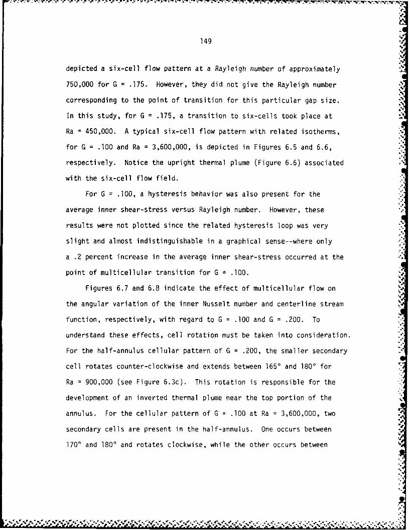
149
depicted a six-cell flow pattern at a Rayleigh number of approximately
750,000 for G = .175. However, they did not give the Rayleigh number
corresponding to the point of transition for this particular gap size.
In this study, for G = .175, a transition to six-cells took place at
Ra = 450,000. A typical six-cell flow pattern with related isotherms,
for G = .100 and Ra = 3,600,000, is depicted in Figures 6.5 and 6.6,
respectively. Notice the upright thermal plume (Figure 6.6) associated
with the six-cell flow field.
For G .100, a hysteresis behavior was also present for the
average inner shear-stress versus Rayleigh number. However, these
results were not plotted since the related hysteresis loop was very
slight and almost indistinguishable in a graphical sense--where only
a .2 percent increase in the average inner shear-stress occurred at the
point of multicellular transition for G = .100.
Figures 6.7 and 6.8 indicate the effect of multicellular flow on
the angular variation of the inner Nusselt number and centerline stream
function, respectively, with regard to G = .100 and G = .200. To
understand these effects, cell rotation must be taken into consideration.
For the half-annulus cellular pattern of G = .200, the smaller secondary
cell rotates counter-clockwise and extends between 1650 and 1800 for
Ra = 900,000 (see Figure 6.3c). This rotation is responsible for the
development of an inverted thermal plume near the top portion of the
annulus. For the cellular pattern of G = .100 at Ra = 3,600,000, two
secondary cells are present in the half-annulus. One occurs between
170' and 1800 and rotates clockwise, while the other occurs between

150
Figure 6.5. Streamlines of a six-cellular
flow field at
Ra = 3,600,000
for G .100 and Pr =
.706(diameter
ratio shown as 1.5 times actual size)

151
Figure 6.6. Isotherms of a six-cellular flow field at Ra=3,600,000 for G = .100 and Pr .706(diameter ratio shown as 1.5 times actual size)
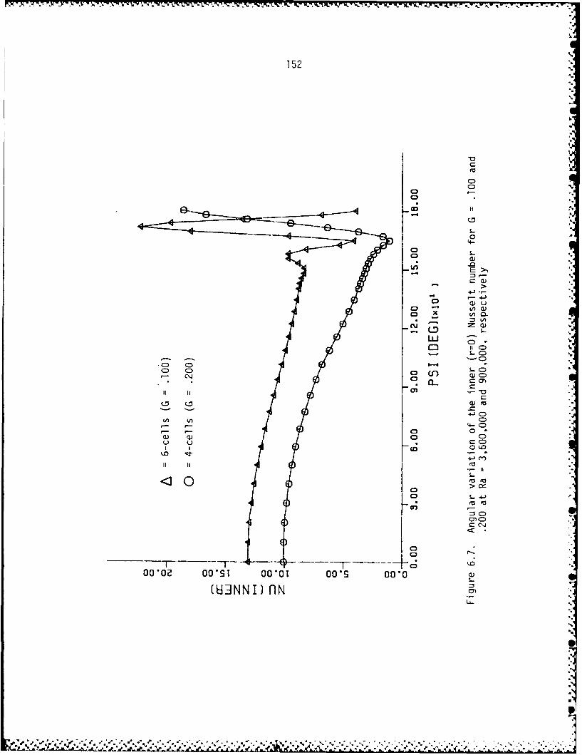
IV VI . = . 1v %.-7k.w.L--,L-cv- R -- - Zo Z-7 ZU- , = -7-4
152
C)
0 -00I- II
0C c
C)a
o -4-'V
LU)SIi 4
C- CJ :)0CD c a)C)4L3i:KY ..
IIc
a0
oe
=3 CD~
0)C
00 *0 OO*s1 GO*Ot 00's 0010 (U
(HINNi) flN
U-U

153
C30
coo
V) a)
CLK D4-
C) x)
C3C
u CD
C)u-ci
L >
-r s- (=
00' 00* 0000 1 0
Lz-'

154
1650 and 170' and rotates counter-clockwise (see Figure 6.5).
Due to the inverted thermal plume for G = .200, Figure 6.7 shows
a local maximum in heat transfer on the inner wall at ' = 180' and a
local minimum near ' = 1650. In contrast, the six-cell flow pattern
of G = .100 shows a local maximum in heat transfer near = 1700 due
to the counter-clockwise rotating secondary cell, while a local minimum
results at ' : 1800. This minimum occurs because the clockwise
rotating secondary cell causes an upright thermal plume near the top
of the inner cylinder. Also, smaller local maximum and minimum in heat
transfer result near ' = 1550 and 1650, respectively, due to the thermal
response of the clockwise rotating primary cell (which bottle-necks)
near ' 155' coupled with the counter-clockwise rotating secondary cell.
In a similar manner, the two types of multicellular flow also cause
a departure of the unicellular sinusoidal-like stream function
distribution between ' = 1500 and 1800. This departure is illustrated
in Figure 6.8 for the four and six-cell flow patterns.
6.1.2. Analytical comparison
The analytical perturbation expressions derived in Chapter 4,
from the finite-Prandtl number boundary-layer equations, were employed
as convenient checks to the pretransitional results generated in the
preceding numerical analysis.
The forthcoming comparison has a dual purpose: first, it is
valuable in the sense that the amount of available data pertaining to
local flow changes in the narrow-type gaps is extremely scarce for the
~.1
,'a' r > ' . J . -I"! -*. ," '-" - .. "-"• •"-" ,"-" "• ".•," *

155
high Rayleigh number range; and second, a valid comparison will serve
to support the numerical method used in this study, which in turn,
supports the asymptotic analysis described in Chapter 4.
The three-term inner Nusselt number perturbation expression given
in Eq. (4.54), together with the three-term expressions for vorticity
and stream function given in Eq. (4.29), will be used to generate
comparative data for the pretransitional 2-D Navier-Stokes numerical
results. Comparisons for the inner (r = 0) Nusselt number, the inner-
wall (r = 0) vorticity and the center-line (r = .5) stream function are
provided in Figures 6.9-6.11, respectively.
Figure 6.9 depicts the angular variation of the inner Nusselt
number using the analytical expression (4.54) with G = 4.0 and Pr = .706.
It is worth noting that G 4.0 does not correspond to a conduction-
dominated flow (as with G = 1.0 or 2.0), but rather a flow subject to
significant convective effects. Recalling that G = Ra /4G, four
different combinations of G and Ra corresponding to G = 4.0 will be
used as numerical comparisons to the analytical result. These
combinations are G = .200 (Ra = 160,000), G = .150 (Ra = 505,680),
G = .100 (Ra = 2,560,000) and G = .025 (Ra = 6.554 x 10⁸). Related
results are also displayed in Figure 6.9.
The best comparison to the analytical result corresponded to
G = .025. This was expected since the asymptotic analysis was tailored
for the small-gap/high Rayleigh number flow regime. Therefore, the 2-D
Navier-Stokes solutions do indeed converge toward the perturbation
solutions as G - 0. In the comparisons that follow, relative errors

156
ES- 0
C3 o 0 ..
+4 CD-
.'1
Lfl (
E 0
- >
LUI
S- C
CD-
U; r-
CD C) CDOXOa) O9o oO
kc c -t u cor_ C4.0 LO - -
C)a l .4tD C)4-
U' -J t

157
of the 2-D Navier-Stokes results with respect to the analytical results
are calculated. For G = .025, a maximum error of 1.5 percent resulted
near the top of the inner cylinder, ' = 1800. The three larger size
gaps also compared favorably. For G : .200, .150 and .100, maximum
respective errors of 11.5, 8.5 and 6.0 percent occurred, also at ' = 1800.
In Figure 6.10, a comparison similar to Figure 6.9 is presented.
This new comparison regards the angular variation of the inner-wall
vorticity for G = 4.0 and Pr = .706. For G = .200, .100 and .025,
maximum respective errors of 7.1, 3.5 and 1.0 percent resulted near
'= 900, or approximately the point of maximum fluid velocity.
Lastly, Figure 6.11 depicts the angular variation of the center-line
stream function for G = 4.0 and Pr = .706. This particular comparison
was in very close agreement to the 2-D Navier-Stokes results, with
maximum respective errors of 2.0, 1.5 and 1.0 percent for G = .200,
.100 and .025.
Although the inner Nusselt number (which is proportional to the
radial temperature gradient) is generally considered the least sensitive
parameter of the three, it did not agree as closely as did the
inner-wall vorticity and the center-line stream function comparisons.
Most probably, this agreement would improve if more expansion terms
are incorporated into the analytical expression for the inner Nusselt
number. But overall, all three analytical comparisons agreed rather
well with the 2-D Navier-Stokes results, hence supporting both the
numerical and analytical work set forth in this thesis.
It

Kj - -
158
0
ES- 00 u4--
C)~ >,
4-) L/n
OS->
C) >
00- - CI.J
C)Li S- 0)
. Lo LO ~ ~0) LO L) 41. -ro to e~ o C a
4-i
0 0D LA 4-.-. ~~, 00C) 00r
11 It 11 0
4-)
eo -
0 -?
* C3' (a 0
0D
44Y0a
O1,1O 0O10 0*0 OP0 00 0 cS.-
OIVM- 3NN-
%

159
0 04- tf
-S.-
ma 0
C)L
.1.
U U
C)) 4
L U (a
4- -. )un
CD (a
CDW 0C)4~
I-C3 ~ w UC
-~4-JCD CDI
-~4-0
0 + -
00 X 00 * a lo U.A -. '
0 0* Osl 00) W0
II '~- w .-
CD 0
160
*, In summary, the first three terms of the perturbation solution
appear to be valid to within approximately 10 percent for the
pretransitional cases of G < .200. Thus, quick and fairly accurate
approximate solutions to the 2-D Navier-Stokes equations, in this
particular range of narrow-gap widths, can be obtained from the
analytical expressions derived in this study.
6.1.3. Small-gap number stability curves
As discussed in Chapter 4, previous investigators (Walton, 1980;
Powe et al., 1971; Liu et al., 1962) speculated that as the narrow
annular gap spacing approaches zero, a true B6nard-type instability
would erupt, corresponding to a critical Rayleigh number (Rab-a) of
approximately 1700. Instead, it appears from Figure 6.12 that the
minimum transitional Rayleigh number approaches 2400 for G = .175.
Beyond this point, the transitional Rayleigh number begins to increase
substantially with decreasing gap number; where at G = .050, the
thermal instability sets in at approximately Raba = 4560.
Directly related to the stability curve of Figure 6.12 is
Figure 6.13, which was obtained from the relation G Ra1/4G. This
new curve appears monotonic and seems to indicate that for very small
gaps, the instability sets in at a near-constant value of G equal to
approximately 3.90.
All data points on the stability curve of Figure 6.12 were
calculated assuming vertical symmetry for a half-annular mesh of
31 x 102 nodes, except for G .100 and .200 where the complete annulus

161
V)
r-o
LA 3
(U
0
0*
IL - ' S.
X 0
'D == a)
.0j '-C (
(U -CO
00
(aC
100
00'h? 0O*O!i 00 9c 00*c 00*92 OOh2
a-
OL)U wm H11A1S

162
-~S-
4-
9Li) C.D4-
-
0(
0
-4-
LrL
CD
U-
V.L
NOII.V

163
(0 - 27T) was considered when investigating possible hysteresis behavior.
The vertical symmetry assumption proved to be valid, as was discussed
in Section 5.2.4. In order to obtain some type of tolerance criteria
for the numerically predicted transitional Rayleigh numbers, a mesh
resolution study was performed (see Appendix E) for three different
size gap widths. Based on these results, it appears that the predicted
transitional Rayleigh numbers are within 5 to 15 percent uncertainty.
This error range seems to indicate fairly reasonable accuracy when
compared to some of the larger discrepancies reported in the literature
for predicting the onset of secondary motion (Elder, 1965; Powe et al.,
1971; Rao et al., 1985).
Also in Appendix E is a comparison of the cellular development
for G = .200 when using either a first-order upwind or a second-order
central-differencing method. This comparison demonstrated that even
at very high Rayleigh numbers, the first-order upwind differencing
scheme could not capture multicellular flow transition. In addition,
this appendix compares mean Nusselt numbers predicted numerically for
G = .200 to that estimated by the correlation of Raithby and
Hollands (1975), which was valid for narrow gaps in the pretransitional
convective-dominated flow regimes, and also to the correlation of
Kuehn and Goldstein (1980b).
6.2. Hydrodynamic Instability
Under certain conditions, an unsteady multicellular flow
instability originates in the vertical sections of two-dimensional
-I- - S.,

164
narrow horizontal cylindrical annuli. This particular type of
multicellular flow was captured numerically from the simplified
governing equations derived in Section 4.5, corresponding to the high
Rayleigh number/narrow-gap/small-Prandtl number limiting conditions.
The multicells apparently result because of hydrodynamic
instability, and are analogous to those investigated by other researchers
with regard to the vertical slot geometry, as discussed in detail in
Section 2.6.
In contrast to the vertical slot studies, the multicellular flow
initiated in the vertical portions of a horizontal annulus is unsteady.
Results from this study seem to indicate that the initial instability
behaves in a rather periodic manner. That is, the strength of the
cells appears to increase and decrease with time in a cyclic fashion.
Closely related to this observation is the phenomena of strange-
attractors. In some systems that experience a multicellular-like flow
instability, an ordered route to chaos has been reported (see Section
2.5 for specific references and related discussion). Briefly though,
a typical sequence of events consists of the system first behaving in
a time-periodic manner, followed by a cycle of periodic-doubling until
finally, the system is stressed into chaotic-like nonperiodic motion.
This present flow under study seems to have the potential to
follow a similar ordered path to chaos.
The following subsections deal with a thorough discussion of both
the numerical and analytical results relating to this unique type of
secondary-flow instability.

165
6.2.1. Pr - 0 numerical solution
Assuming synnetry about the vertical center-line greatly reduced
the amount of CPU-time associated with the numerical computations.
This assumption was based on the detailed discussion given in Section
5.2. The above symmetry condition was proven valid in Figure 6.14a.
Here, the first 832 time steps (for At = 1.0) of the numerical solution
to the complete annulus (31 x 202 nodes) produced the cellular cycle of
the half-annulus (31 x 102 nodes) almost identically, and graphically,
no notable differences could be discerned. Also, for both the full and
half-annulus, the inner-wall vorticity at t = 832 were compared in
Figure 6.14b. The two cases were again in close agreement, to within
approximately one percent error. Note that these curves are presented
at this time to support the assumption of vertical symmetry. The exact
nature and meaning of the cellular behavior described by these curves
will be explained later in this section. Therefore, for the results
that follow, a half-annulus mesh of 31 radial nodes and 102 angular
nodes was employed. In general, the justification for this size mesh
was due to proper resolution of the cellular structure and also to
computer power and time limitations. These considerations are again
discussed in more detail in Section 5.2.
Steady-state results were obtained up to a G value of 5.1. Then,
at G = 5.2, a seven-cell unsteady instability set in at a t value of
approximately 30.0. Note that the converged steady-state results for
G = 5.1 were used as initial conditions to start the G = 5.2 case.
Prior to the seven-cell development, the instability first occurs near
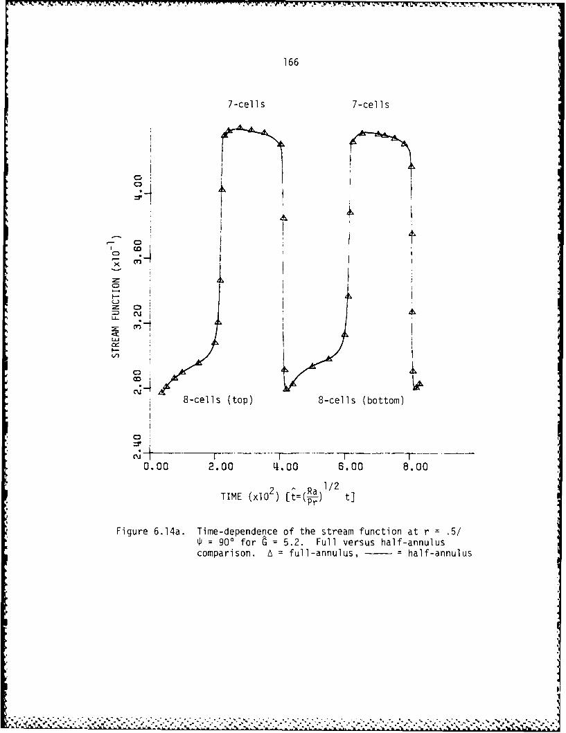
S. ~ ~ ~ ~ V W . I
166
7-cells 7-cells
o~r
C)
0,
CT -4
0.00 2.00 41.00 6.00 6.00
TIME WxO 2) [tI(L 11 t]
Figure 6.14a. Time-dependence of the stream function at r .5/S=90' for =5.2. Full versus half-annulus
comparison. A full-annulus, =half-annulus

167
C,,
oc
CDC
C) <4QD c
0 - I
0
C-0
3-
0o (f) C
CT)O
4- C:
0
> In
L
i
OV- C
CD~
09009,0 olf h ~ 0,0 f0l
L.
-t-

168
= 90, where the maximum buoyancy force causes the most rapid rising
and falling of the fluid, as illustrated in Figure 6.15a. Also in
Figure 6.15b, the cellular pattern is displayed at a time slightly
beyond the initial development stage. The cellular instability then
grew until the relatively stable seven-cell pattern resulted at
t = 30.0. The initial seven-cell solution encompassed an arc of about
80 degrees near the vertical portion of the annulus (see Figure 6.16).
It is important to note that this multicellular flow instability
was preserved with both finer and coarser mesh sizes, as evidenced by
the data in Table 6.1. The coarser mesh, 31 x 72, could not resolve the
smaller cells near the top and bottom portion of the vertical section,
thus resulting in only five cells for the initial instability. The
other three mesh sizes indicate that the instability sets in as a six
or seven-cellular flow pattern. This result was in close agreement with
that reported by Lee and Korpela (1983) for their vertical slot geometry.
Table 6.1. Mesh resolution comparison
Mesh G Geometry Cells Convergence Precisionsize transitional constraint
31 x 72 5.7 half-annulus 5 1 x 10⁻⁶ single
31 x 102 5.2 half-annulus 7 1 x 10⁻⁶ single
41 132 4.9 half-annulus 7 1 x 10⁻⁸ double
31 162 5.2 full-annulus 6 1 x 10⁻⁶ single
~.t

Wit~~~~~~~~~ ~ ~ ~ ~ ~ ~ ~ KY. 1pplvk- N.1F-r 1W -,VI-1 1A .
169
-----------
Figue 615a Stramlnesof a intia devlopentstag fo th
onse of ydrdynaic nstailit atG 5. an
21.0 (diaeterrati 1.5

- 4~.~*~ . - - - - - A . . . - - -. .
170
p
AhA
A
p
4,.
a'.
p
pp4-
.4
I.
P4.
Figure 6.15b. Streamlines of the cellular instability slightlybeyond the initial development stage for G 5.2and t = 25.0 (diameter ratio = 1.5)
-a'.
a
9
~:~.-* .* *A.* -'- .- -

171
Figure 6.16. Streamlines of the initial seven-cellular flowfield for G=5.2 and £=35.0 (diameter ratio=1.5)
S. k.A
172
They claimed that a six-cellular flow pattern initially appeared at
Grb-a = 8000 for a Prandtl number very near zero (see Section 2.6).
This Grashof number of 8000 compared favorably with the transitional
value of this study, where G = 5.2 translated to a Grashof number (based
on gap width) of 7855. Furthermore, transitional values of 7880 and
7932 were predicted analytically by Vest and Arpaci (1969) and Korpela
et al. (1973), respectively, for a similar vertical slot geometry.
Lee and Korpela (1983) also reported a wavenumber of 2.80
associated with the six-cellular flow pattern in their narrow vertical
slot. They defined the wavenumber as 2n/Z, where Z represented thecenter-point distance between two adjacent cells. When this study's
initial seven-cellular state at t = 35.0 was compared to their narrow
vertical slot geometry (aspect ratio = 15), the wavenumber was
determined to be approximately 2.60--a good correlation.
However, as previously mentioned, the cellular flow within the
vertical slot geometry was steady, whereas in this study, the
multicellular flow at G 5.2 seemed to vacillate periodically about
the seven-cell state. That is, upon increasing t, a cyclic pattern
resulted: an additional eighth cell formed on top of the 800 arc,
reverted back to seven cells, then an additional eighth cell formed
on the bottom of the 800 arc, and again, reverted back to seven cells,
forming an 8-7-8-7 cellular pattern (see Figure 6.17). In the
seven-cell formation, the stronger cells appeared near i= 900 (see
Figures 6.16 and 6.18). The remaining cells successively decreased in
strength (in approximate proportion to sin ) as they proceeded away
S -- - i.

~W. ~ V~~Wr.'FV ~ ~ It~ ~!~YJ'~..WJdjF1W~v " M yv PVT Av-,% lvw -W- Fr - v-, rr
173
0
LIL- 1
'00
- D0
. LO,00
0 LUj
u 0 L0
C) L -C)
0
cucoo
ojrUC,
E 0:
0C)
U
(OLx) NQIIJNlA WV38iS
~ . ~ *~*~,* ~ ~ ~~ *~ /~/\ * *~ ~'%

174
C3C
LLLiuw
CD
4E) C) Li
- -e
&& 42 C
ELi
-e CD,
- > -
o h 60 2001001
(A I-1H~NA L-

175
from the 90° point.
At the start of the cellular cycle, the seven cells weakened (the
maximum stream function decreased) as the eighth cell formed on top
(see Figure 6.19). Then, the eight-cell pattern grew in strength until
the two larger cells near 90' merged into one with the maximum stream
function shifting upward to 92', thus forming an upward-shifted seven
cellular flow pattern. Similarly, these seven cells then weakened as
the eighth cell formed on the bottom portion of the chain of cells
(see Figure 6.20). Again, the eight-cell pattern grew in strength until
the two larger cplus merged into one with the maximum stream function
shiftinq downwards now to 87', thus forming a downward-shifted
seven-el luldr flow pattern completing the 8,-7-8-7 cycle. A cycl1(
behavl()r ,)f th,, avera(je inner shiear-stress also accompanied this
hanq]jnq el lular pdttern. Table b.c' outlines a typical cycle.P
ot9 thdt tnese relations hi;s would rePeat for subsequent cycles.;"J.
Table b.2. 1horacteristlcs of the 8-7-8-7- cellular cycle
(,el 1 t Average Maximum Maximumstructure inner stream function stream
shear-stress location function value
8-top 85.0 .23722 870 .4506
7-top 280.0 .23644 92"' .4815
8-bottom 350.0 .237247 82' .4501
7-bottom 680.0 .23627 870 .4824
°,
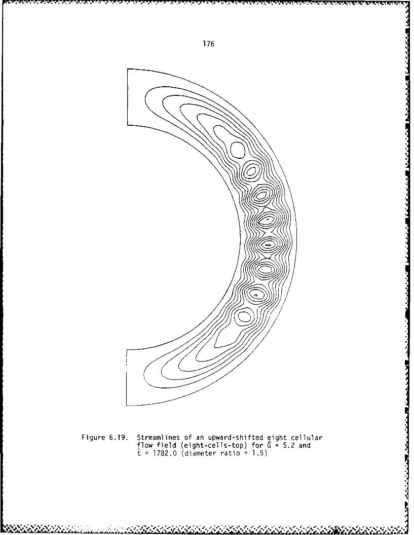
176
Figure 6.19. Streamlines of an upward-shifted eight cellularflow field (eight-cells-top) for G 5.2 andt 1782.0 (diameter ratio 1.5)
U ,,,.,.1~ -U' ,b.

* ~ ~ ~ ~ r .. T vv.M h- a . aa
177
J
Figure 6.20. Streamlines of a downward-shifted eight cellular* flow field (eight-cells-bottom) for G =5.2 and
t 1182.0 (diameter ratio 1.5)

178
This table, along with the particular nature of the cellular activity,
seems to imply a potential energy exchange in the 8-7-8-7 cellular cycle.
That is, the most potential energy seems to be stored within the seven-
cell formation, corresponding to a minimum average shear-stress and a
larger maximum stream function. It then appears that some of the
potential energy is released and is converted to shear energy which aids
in the creation of an eighth-cell. This then causes a rise in the
average inner shear-stress and a corresponding decrease in the maximum
stream function.
The strength of the stream function at ' : 90'/r = .5 behaved in
a square-wave-like time-periodic fashion, as clearly illustrated in
Figure 6.17. The period of this cyclic pattern was approximately 800
time (t) units.
The fact that the cellular behavior at G = 5.2 is unsteady can be
supported by the work of Thomas and Vahl Davis (1970). They observed
a multicellular flow, similar to that reported by Elder (1965) and
Lee and Korpela (1983), in narrow vertical cylindrical annuli (see
Section 2.6). Even though they were only interested in predicting
the onset of this multicellular flow, they did report that the flow
was unsteady and attributed this unsteadiness to curvature effects.
Figure 6.21 displays the vorticity distribution at the inner
cylinder wall for both unicellular and multicellular flows. The
unicellular steady-state result, for G = 5.1, behaved in a sinusoidal
manner with the maximum vorticity occurring near 4 = 900. Then, due to
the multicellular instability at G = 5.2, the vorticity distribution
... '. , . -. . Z.'.,, .. j.' '-. - - - - ... - . - - - . -.- -.- , - .'.°....-.- - .' .#.''-s

~~mJ ~ ~ " Y7v-r hP7 r-P rF 'y" W 'J \P
179
C3.
a0
CDCDA
C~j LU
o1 -~ C).
V C)
00C3
0D 0 ea
y ' I... C3l)
0t 11 c IV
S0 +~
Lflm -I I 03
N % %

180
was clearly disturbed and behaved in an intense oscillatory manner near
the vertical portion of the half-annulus. This extremely wavy
vorticity pattern shifted only slightly as the number of _e',..>-
transition from eight-cells-top, to seven-cells, t., e -
The seven-cell solution experienced the strongest variatl:n wa'
vorticity. For individual comparison, the four curves < .
Figure 6.21 are depicted separately in Fiq, ures 6. :" -, .
To examine the change in cellular enar - .
5.5 was calculated using the G = 5.2 seven-_el>Id',a .
at t = 35.0. Figure 6.26a displays t.ne :wle .ar- .
function at 90'/r = .5, using a ,constir*t 1-it,
to t = 400, a hint of double-periodl(-lt, seer - :, ..
afterwards, the flow seems to become ader -)jl .,-,,,- .
of chaotic motion. The multicellular atterr wa'
G = 5.2, except in this case, the cei ,lar :,, .-it
between nine, ten and eleven cells. The -da !- "-.ur
occurring near 'Y = 90', was greatest for the n , it- .
least for the eleven-cell structure A t: V i LI '-,
is shown in Figure 6.26b. Also, in general, t, ,,
G= 5.5 was similar to that experienced witn -
The preceding results show that a multicellIfl,, :,
instability is indeed probable in the vertical se,-tns ,,
horizontal annuli. It appears that this instabilit, drs, e , ,
of the coupling of the nonlinear terms with the buoyancy ter•
"71

-4-v
dr c494
4 A
ANC~

-Al" 113 THE NMERICAL AND ANALYTICAL STUDY OF BIFURCATION AND 3/3HULTICELLULAR FLOGI..(U) AIR FORCE INST OF TECHNAIANT-PATTERSON AFD ON4 0 FONT 1907
UNCLSSIFIED AIFIT.'CI/MR-97-1340 F/G 20/13 ML
,loss EEEEE
ILI R WT IW~iLl W wl.TIiM4
2.2.
11111*' 5IL 1 1112.0
iii1.05 1111 . 11 1.
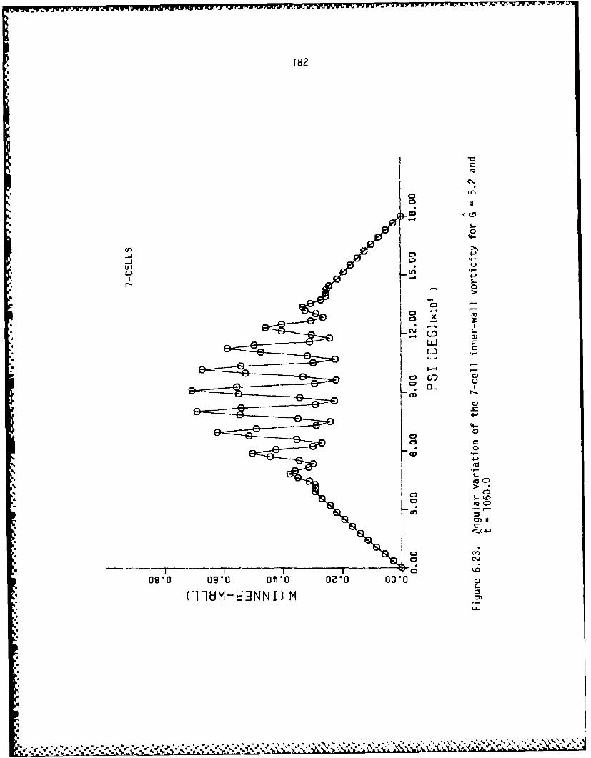
182
0
o3L
4-0
CY)
UIIEI-6(f) I )

183
co <CD
a.. 4--
-J 19
I oo o
>~ .
C3C
Lo
.00
U-)
C"C
4--
~010~I
>CD
0S C\J
08.0 0910 ohO *0 020 0010
(TlHMH NNI) MS.-
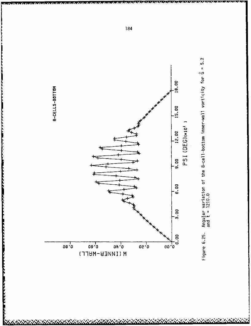
184
o1 0
too
00
0
-44
ov .
1S--
o (to
0)
0910019 0 Ol *0 210 0 *
LA-S
te'0

185
04-
C3
L9
11
i II 4--
0
C C
0 .
LC
-- 4-09*0 Oslo Ob*O 0610 0210
C\1
NoI1oNl WOKS %D

186
Fiue62b9temie fa eee-ellrfo il o
G9 . n 010(imtrrto=15

187
-G sin P, in the vorticity equation. Considering this statement
together with the fact that periodicity is iJst for G = 5.5, one might
infer that the effects of the nonlinear terms become more and more
pronounced as G increases.
Based on this reasoning, it is anticipated that for some
intermediate value of G between 5.2 and 5.5, the possibility of an
emerging doubly-periodic solution is likely, thus causing the system
to make a further transition on its ordered path to chaos.
6.2.2. Pr - 0 perturbative solution
To verify the Pr - 0 perturbative expansion solution, the
analytical results will be compared to related numerical results for
the pretransitional case G = 5.1. As discussed in Section 4.6, only
F1 and W, (as given in Eqs. (4.93) and (4.94), respectively) appear to
be significant prior to the onset of multicellular flow. This claim
will now be tested in the following comparisons.
An analytical expression for the inner wall vorticity was found
by evaluating Wl at r = 0 for G = 5.1:
Winner .425 sin
A comparison to the numerical result at G 5.1 is given in Figure
6.27. The largest deviations occurred near = 45 and 1350,
corresponding to relative errors of nearly five percent. At the point
of maximum vorticity, P 900, the error was only about .1 percent.
-,U " '' " 3 . " "" ° - . ' "
.°. - - . " -' . " - - " . ' - . " - . - . .

188
S-
o
-JO
-
u CC
-~ -4 xa
CC
LU,
CU
CYa)
4--
0:<.C3C
(-1-13M-H N I
189
Similarly, an analytical expression for the vorticity at the
horizontal center-line was obtained by evaluating Wl at ' 900 and
G= 5.1:
W = 2.55 (r2 _ r +
This result was compared to the numerical result in Figure 6.28. The
vorticity was positive near the walls of the annulus, .81 < r < .19,
signifying the boundary-layer region. It became negative within the
center portion of the annulus, representing the inviscid-core region.
A maximum error of approximately 3.5 percent occurred near the
switching point, where the vorticity changed from positive to negative.
The maximum vorticity occurred at the walls, r = 0 and 1, and took on
a value of approximately .425. For r = .5, the vorticity reached a
minimum at -.2125.
The analytical expression for stream function at ' 900 and
G = 5.1 is given by:
F90o- 5.527125 r2 (r - 1)2
Figure 6.29 displays its comparison to the numerical result. A
maximum error of about one percent occurred at r = .5, where the
stream function reached its maximum value of approximately .346.
The above results indicate that the pretransitional flow field
(G < 5.1) can be adequately represented by the first-term expansions
% N

190
S-'
0
go
4J.
lo C)
o -i
00
0 4
0r~ U 43
E e
r_. >o C3.r
e C0
0210O~ 0010 0210- 01110-
AlDI ibOA

191
LO
S-
*00
0
0 ~4-)
44
C)~
11 1
II

192
(W1 and Fl) of the perturbation solution, which do not account for
nonlinear effects. That is, the problem appears to be linear and steady
up to G = 5.1. This suggests that the full nonlinear influence only
becomes evident just prior to and beyond the point of instability. For
this case, the nonlinear effects appear to come into play for G > 5.2.
Figure 6.30 was generated in order to show how the Pr - 0
perturbative solution breaks down as the Prandtl number increases.- pr1/4,
Using the relationship G = G Pr , two numerical results corresponding
to Pr = .7 and 2.0 were compared to the analytical solution for G = 4.0.
Surprisingly, for Prandtl numbers as large as 2.0, the comparison
between the analytical and numerical results was fairly close. For
Pr = .7 and 2.0, respective maximum errors of 3.5 and 10.5 percent
occurred near = 1400. Thus, for air, the use of Pr - 0 expansions
should provide for relatively good estimates of the local flow
variables, at least for the pretransitional cases.
The finite-Prandtl number perturbative solution of Eq. (4.29) can
also be used to obtain analytical results for small Prandtl number cases.
Using the three-term perturbative solution (F1 , F2 and F3 ), all of the
important physics can be taken into account, including the first effects
of nonlinearity through F2 and F3. For liquid mercury, Pr = .02, a
six-cellular counter-rotating flow was encountered at G = 3.5. In the
complete annulus, the large kidney-shaped cells maintained themselves
near = 90 and 2700, while two smaller counter-rotating cells formed
first at the bottom, then at the top portions of the annulus - Y' = 0 and
1800. This multicellular flow pattern was more fully developed for
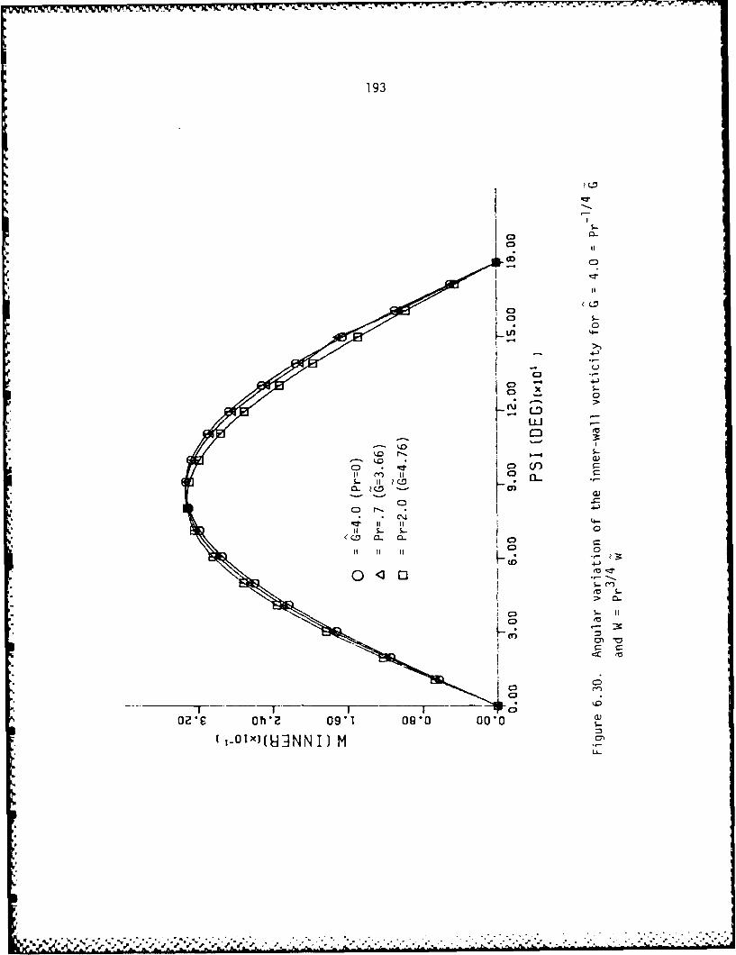
193
IF C:)
0
0n
C)-
uco
S.- if If 4
<~ 11 - S-
00
.,- (n-
(o S..
0n -
cm r-
ozc Oh 0911 90 0* a)
-Olxl(HIJ.NN I] M

194
G= 4.0, and is depicted in Figure 6.31. This particular flow pattern
was very similar to that observed by Mack and Bishop (1968) and Huetz
and Petit (1974) for a larger gap width, G = 1, and Pr = .02. They
graphically depicted the multicellular behavior at Ra = 300, but
mentioned that it initially occurred (analytically) at a lower value of
Rayleigh number. In addition, the presence and shape of the secondary
cells for G = 1 and Pr = .02 were confirmed by the numerical experiments
of Charrier-Mojtabi et al. (1979), where they reported a similar type of
multicellular flow that began to develop near Ra = 300.
Using the relation G = Ra1/4G, G = 4.0 translates into a Rayleigh
number of 256 for G = 1.0, thus reaffirming the results described above.
Note also that Huetz and Petit (1974) claimed that the bottom cell
developed first. However, when the finite-Prandtl number boundary-layer
equations were solved numerically for Pr = .02 (thus incorporating the
full effects of nonlinearity), a multicellular flow field resembling
that described with the Pr - 0 numerical solution resulted in the
vertical section of the half-annulus at G = 1.92 (G = 5.106).
From these results, one might conclude that the effects of the
boundary-layer are less significant in the larger size gaps, thus
creating a weakly nonlinear instability as originally reported by
Mack and Bishop (1968). But for the narrow-gap widths, the boundary-
layer effects are much more dominant, thus creating stronger nonlinear
interactions which trigger the hydrodynamic type of instability as
described in this study for the small-gap/small-Prandtl number limiting
conditions. These results are discussed further in Appendix B.

195
Figure 6.31. Streamlines of the steady six-cellular perturbationsolution corresponding to Pr = .02 and
= 4.0 (diameter ratio = 2.0)

196
6.2.3. Small-Prandtl number stability curves
In order to obtain a more universal relationship for predicting
multicellular flow instability with regard to small-Prandtl number
fluids in the narrow horizontal annuli, the following derivation was
considered.
It was shown in Chapter 4 that
SRa 1/ 4 G = Pr I / 4 G (6.1)
but since Ra = Gra Pr, Eq. (6.1) becomes (after some manipulation):
4.4
Gra = G (6.2)
where Gra is the Grashof number based on the inner cylinder radius.U.
Then, using the relation
Grb-a =Gra
one obtains:
Grb-a G (6.3)
where Gr b-a now represents the Grashof number based on the gap width.
For Pr = 0, the transition to multicellular flow occurred at G = 5.2.
Using this result transforms Eq. (6.3) into a universal relation which

197
is inversely proportional to the gap number, G:
Grba 731 (6.4a)ba G
This relationship is plotted for various values of G in Figure 6.32.
Note that the transitional value of Grba 8000, as predicted in this
study and by Lee and Korpela (1983), corresponds to a gap number of
approximately G = .10. Also, the shape of the stability curve seems to
make sense, since for the vertical slot studies it was reported by Lee
and Korpela (1983) and Elder (1965) that as the gap width increased, the
transition to turbulence occurred sooner. Similarly, in this study, it
was shown for very small-gap widths (for air) that as the gap number 5
decreased, the transitional Rayleigh number for multicellular flow
increased. The above statements indicate that as gap width decreases,
the onset of instability is suppressed. Thus, the stress parameter G
or Rayleigh number, must increase accordingly in order to trigger the
respective hydrodynamic or thermal instability. Qualitatively, the shape
of the stability curve in Figure 6.12 for Pr = .706 (in the small-gap
limit) is similar to that in Figure 6.32 for Pr 0 0. Also, for thermal
instability, the following relation holds:
'4Grb-a G • Pr
where for air in the small-gap limit, Pr .706 and GTR 4.0, hence:
Grba air _)363air - (6.4b)
lair

198
CD~
* E
C3C
100
C3 -0V 0)'4--
I -
cc 0
C 0'
Lo
a -
0 '4-)
-Q
. C
-T*. T C a
00*2c~~~~~ ~ ' 00*12 0.1 0* 00S
(,OLX UawN JOSV..

199 p
This relationship is very similar to that for hydrodynamic instability
(Pr = 0), except the proportionality constant differs by a factor of
two.
Taking the above approach a step further, one can also determine a
stability curve based on finite-Prandtl number by using the relation
G= 5.2 PrI/4, where G = 5.2 again represents the transitional value for
Pr = 0. The new stability curve is shown in Figure 6.33. These
analytical predictions were compared against numerically predicted
transitional values of G (obtained from the finite-Prandtl number
boundary-layer equations) for four different small-Prandtl number fluids
(see Table 6.3).
Table 6.3 indicates that for small-Prandtl numbers, the
relationship G = 5.2 Pr1/4 appears to be valid for predicting the
transitional G associated with hydrodynamic instability in the vertical
sections of narrow annuli. For Pr .02, an initial seven-cell unsteady
flow field, resembling that of Pr 0, was obtained at G = 1.92.
Table 6.3. Numerical predictions of G transitional as a function ofPrandtl number
Prandtl number G (transitional) G(= GPr-I/4
.02 1.92 5.106
.2 3.42 5.114
.3 3.80 5.135
.35 3.99 5.187

200
1%
0
M
0
S..
* C) Cl
IL 4-W
-E S
r--4
%0tzz-
S- u
C) c4-
V)
S-Cosle ~~ ~ ~ ~ =oe O* oe O'
NOUISMI -

201
However, for Pr = .35 (at G = 3.99), an interesting change occurred--
only a six-cell pattern resulted (see Figure 6.34) and the solution
achieved a steady-state condition similar to that reported for the
cellular instability between narrow vertical slots. Also, at Pr = .35,
the isotherms were no longer perfectly concentric as with the Pr = 0
solution. Instead, they responded quite closely with the fluid motion
(see Figure 6.35).
From these results, it appears that the same type of hydrodynamic
instability as for Pr = 0 extends to at least Pr = .35. But, the nature
of the multicellular flow has changed from seven-cells unsteady for
Pr = .02 to six-cells steady with Pr = .35. Perhaps, though, if one
stresses the Pr = .35 case past G = 3.99, an unsteady cellular motion
may ensue. Note that for Pr = .2 and .3, the cellular flow field was
not resolved; only the point of instability was determined.
The two stability curves described above should provide for simple
and convenient comparisons to future related studies of narrow
horizontal annuli (especially experimental ones). Note that the curve
in Figure 6.33 could easily be extended for comparison to data in the
larger Prandtl number range, thus, eventually establishing an
acceptance band on this asymptotically generated stability curve.

202
Figure 6.34. Streamlines of the steady six-cellular flow fieldfor Pr .35 at G=3.99 (diameter ratio 1.5)
'I

'aA
,5%*
203*0
5'
a'
SI
a,Aa,ag
a
.5'
5'
5,
.5
5-
-t
-5
5%
'5'a
Figure 6.35. Isotherms of the steady six-cellular flow fieldfor Pr .35 at G = 3.99 (diameter ratio 1.5)

204
7. CONCLUSIONS
Numerical solutions of the 2-D Navier-Stokes equations yielded
steady laminar multicellular flow for air near the top portions of
narrow horizontal isothermal concentric cylinders. It was shown that
hysteresis behavior exists for G = .100 and .200, with regard to sudden
changes in the mean Nusselt number and average shear-stress as the
Rayleigh number was slowly increased and then decreased past the
multicellular transition point. Also, for G less than approximately
.175, the results for air indicate that the transitional Rayleigh number
increases as the gap number decreases. The minimum transitional Rayleigh
number occurred at Rab-a = 2400 for G = .175.
In performing this multicellular flow study, first-order upwind
differencing of the nonlinear convective terms proved inadequate. In
relation to the pretransitional flow field cases, the first-order
method was in good agreement with the results obtained from the
second-order central-differenced numerical scheme. However, for the
higher Rayleigh number flow regimes, the artificial viscosity
associated with the first-order differencing of the nonlinear convective
terms suppressed the development of secondary counter-rotating cells.
Thus, it appears that at least second-order accuracy is needed to
properly capture multicellular flow behavior. Moreover, multicellular
flow resolution is also strongly dependent upon mesh size. That is,
coarse meshes frequently failed to resolve the multicells, while
finer meshes would sometimes result in asymmetric cellular patterns

~~A ~ y.~J.- 3.. - -
205
when not enough nodes were concentrated in the thermal plume region
for air.
A high Rayleigh number/small-gap asymptotic expansion theory was
constructed which simplified the 2-D Navier-Stokes equations intoCartesian-like boundary-layer equations. Analytical perturbative
solutions to these equations were obtained and the results compared
favorably with the pretransitional numerical data generated in the 2-D
Navier-Stokes hysteresis study of this thesis. For the limit as
G - 0, the boundary-layer equations reduced to viscous-dominated
Stokes-flow equations, as shown in Chapter 4. This implies that for
either Ra - 0 or G - 0, a conductive-dominated flow results.
In addition, simplified limiting equations for Pr - 0 and Pr -
were obtained from the finite-Prandtl number boundary-layer equations.
In the Pr limit, only the nonlinear terms in the energy equation
remained and the vorticity equation reduced to a Stokes-flow equation,
suggesting the possibility of a Benard-type thermal instability, as
seen with air near the top portion of narrow annuli. In direct
contrast, the energy equation decoupled from the vorticity equation
and reduced to simply T = l-r for the limit as Pr - 0. Thus, only the
nonlinear terms in the vorticity equation came into play, suggesting
a source of hydrodynamic instability.
When the Pr - 0 equations were solved numerically, an unsteady
time-periodic multicellular instability developed (at G = 5.2) in the
vertical portions of a narrow horizontal annulus. Both the wavenumber
and the transitional Grashof number (based on gap width) of the

.4 W W W -V~ W. - - - - - - - - - - --- i- - _I_%VI'j~ -
206a
initial seven-cellular instability compared favorably with the steady
six-cellular instability experienced in a narrow vertical slot of
aspect ratio equal to 15, as studied by Vest and Arpaci (1969) and
Lee and Korpela (1983).
Upon increasing time, cyclic changes in the multicellular flow
pattern resulted for G = 5.2, forming an 8-7-8-7 repetitive cellular
behavior. However, this periodic flow pattern was lost when G was
increased from 5.2 to 5.5, resulting in a seemingly chaotic cellular
behavior between nine, ten and eleven cells.
Also, the Pr - 0 analytical pretransitional solutions were in
good agreement with the numerical results up to G = 5.1. Based on this
comparison, the Pr - 0 problem appeared linear and steady prior to the
point of instability.
Moreover, a universal relationship for small-Prandtl number
fluids,
Grb-a _731b-a G
was suggested as a simple guide for predicting the onset of
hydrodynamic instability between narrow vertical slot-like geometries.
Figure 6.13 shows that for air (Pr = .706) in very narrow-gap
widths (G < .075), thermal instability sets in near G = 3.90. But for
Pr = 0, hydrodynamic instability sets in at G = 5.2, which corresponds
to a G of approximately 4.8 for air when using the analytical relation
G 5.2 Pr1 /4. This difference in G indicates that the mechanism which
-4

206b
triggers the instability for air is different than that for Pr : 0 (as
previously discussed), and is probably largely due to the nonlinear
terms in the energy equation being coupled with the buoyancy termT
cos in the 2-D Navier-Stokes equations (see Appendix B).
Considering the above, competing effects of both thermal and
hydrodynamic instability may result for Prandtl numbers between zero
and .706.
In order to more fully support and study the nature of the
unsteady multicellular instability described in this research effort,
an experimental analysis of a narrow horizontal annulus filled with
liquid mercury (Pr = .02) is recommended as a possible follow-up
project. Also, numerical solutions relating to G = 5.3 or 5.4 should
be carried out to determine if a doubly-periodic cellular behavior does
indeed precede the chaotic state noted at G = 5.5, as suggested in
the 'ordered path to chaos' scenario described by Ruelle and Takens
(1971).
In addition, the energy spectrum of the fluid motion at G= 5.2
and 5.5 could be calculated in order to reveal any type of spectral
broadening (or fundamental frequencies) associated with flow changes
from time-periodic to chaotic-like behavior.
Lastly, the Pr boundary-layer equations should be solved
numerically to determine the nature of any cellular instability that
might develop. In the same spirit, the limiting 2-D Navier-Stokes
equations derived in Appendix B should also be further investigated
numerically for different size gap widths.
.J.
4' > ,-,- > ," -', -,? _'< - ',:', ,j';' ,' '. -' ' ' '%' ." '+, .'-' -. ' +..-o'.'.'.-..'. '.-,€, '..,-." - .,-

IU - - ,
207
In closing, since natural convective flow instabilities generally
develop slowly, especially in narrow horizontal annuli where the
geometry itself limits the number of degrees of freedom, a more
thorough investigation of laminar flow transition can be undertaken.
Also, it has been conjectured that the transition to chaos in a system
with many degrees of freedom (such as a fluid flow at large Reynolds
numbers) is not qualitatively different from the transition to chaos
in a system with a few degrees of freedom (Jensen, 1987). Thus, it is
hoped that further study of simple geometries, such as described in
this thesis, will lead to a deeper understanding of the nonlinear
processes involved in the mysterious, yet ever-present dynamics of
fluid flow instability phenomena.

208
8. REFERENCES
U
Abbott, M. R. 1964. A numerical method for solving the equations ofnatural convection in a narrow concentric cylindrical annuluswith a horizontal axis. Quart. J. Mech. and Applied Math. 17:471-481.
Arakawa, A. 1966. Computational design of a long-term numericalintegration of the equations of fluid motion: Two dimensionalincompressible flow. J. Comp. Phys. 1:119-143.
Arpaci, V. S. and P. S. Larsen. 1984. Convection heat transfer.Prentice-Hall, Inc., Englewood Cliffs, New Jersey.
Astill, K. N., H. Leong and R. Martorana. 1979. A numerical solutionfor natural convection in concentric spherical annuli. R-1028.The Charles Stark Draper Laboratory, Inc., Cambridge, MA.
Benjamin, T. B. 1978. Bifurcation phenomena in steady flows of aviscous fluid. Proc. R. Soc. London, Ser. A, 359:1-26.
Benjamin, T. B. and T. Mullin. 1982. Notes on the multiplicity offlows in the Taylor experiment. J. Fluid Mech. 121:219-230.
Bird, R. B., W. E. Stewart and E. N. Lightfoot. 1960. Transportphenomena. John Wiley & Sons, Inc., New York.
Bishop, E. H. and C. T. Carley. 1966. Photographic studies of naturalconvection between concentric cylinders. Proc. Heat Trans.Mech. Inst. 63-78.
Bishop, E. H., R. S. Kolflat, L. R. Mack and J. A. Scanlan. 1964.Convective heat transfer between concentric spheres. Proc. HeatTrans. Mech. Inst. 69-80.
Bishop, E. H., L. R. Mack and J. A. Scanlan. 1966. Heat transfer bynatural convection between concentric spheres. Int. J. Heat MassTrans. 9:649-662.
Bishop, E. H., C. T. Carley and R. E. Powe. 1968. Natural convectiveoscillatory flow in cylindrical annuli. J. Heat and Mass Trans.11:1741-1752.
Boyd, R. D. 1981. A unified theory for correlating steady laminarnatural convective heat transfer data for horizontal annuli.Int. J. Heat Mass Trans. 24(9):1545-1548.
. . .. . . . . . . ..

209
Brandst~ter, A., J. Swift, H. L. Swinney and A. Wolf. 1983. Low-dimensional chaos in a hydrodynamic system. Phys. Rev. Letters51(b):1442-1445.
Busse, F. H. and R. M. Clever. 1981. An asymptotic model of two-dimensional convection in the limit of low Prandtl number. J.Fluid Mech. 102:75-83.
Caltagirone, J. P., M. Combarnous and A. Mojtabi. 1979. Naturalconvection between two concentric spheres: Transition towardsa multicellular flow. Proc. of the First Int. Conf. on NumericalMethods in Thermal Problems, Pineridge, Swansea, U.K.
Chand, J. and D. Vir. 1980. Natural convection heat transfer fromhorizontal cylinders. IE (1) J.-CH. 60:34-40.
Chandrashekar, B., P. Vasseur and T. Hung Nguyen. 1984. Naturalconvection in a heat generating fluid bound by two horizontalconcentric cylinders. The Can. J. Chem. Eng. 62:482-489.
Charrier-Mojtabi, M. C., A. Mojtabi and J. P. Caltagirone. 1979.Numerical solution of a flow due to natural convection inhorizontal cylindrical annulus. ASME J. Heat Trans. 101:171-173.
Cho, C. H., K. S. Chang and K. H. Park. 1982. Numerical simulationof natural convection in concentric and eccentric horizontalcylindrical annuli. ASME J. Heat Trans. 104:624-630.
Choi, I. G. and S. A. Korpela. 1980. Stability of the conductionregime of natural convection in a tall vertical annulus. J. FluidMech. 99:725-738.
Chou, F. C. and G. J. Huang. 1984. Combined free and forced laminarconvection in horizontal rectangular channels for high ReRa. TheCan. J. Chem. Eng. 62:830-836.
Clausing, A. M. and S. N. Kempka. 1981. The influences of propertyvariations on natural convection from vertical surfaces. ASMEJ. Heat Trans. 103:609-612.
Clever, R. M. and F. H. Busse. 1981. Low-Prandtl-number convectionin a layer heated from below. J. Fluid Mech. 102:61-74.
Cliffe, K. A. 1983. Numerical calculations of two-cell and single-cell Taylor flows. J. Fluid Mech. 135:219-233.
Coles, D. 1965. Transition in circular Covette flow. J. Fluid Mech.21:385-425.
**% .~ % * % * ~ ** . . - . .
~ ~,* *% - ]

210
Crawford, L. and R. Lemlich. 1962. Natural convection in horizontalconcentric cylindrical annuli. I&EC Fund. 1(4):260-264.
Currie, I. G. 1974. Fundamental mechanics of fluids. McGraw-Hill,Inc., New York.
Custer, J. R. and E. J. Shaughnessy. 1977a. Thermoconvective motion oflow Prandtl number fluids within a horizontal cylindrical annulus.ASME J. Heat Trans. 99:596-602.
Custer, J. R. and E. J. Shaughnessy. 1977b. Natural convection inliquid metals in an enclosure. ASME J. Heat Trans. 99:675-676.
Daniels, P. G. and P. M. Eagles. 1983. Slender channel theory in flowbetween two cylinders. J. Eng. Math. 17:125-147.
Eagles, P. M. 1974. On the torque of wavy vortices. J. Fluid Mech.
62(1):1-9.
Edelson, E. 1986. The ubiquity of nonlinearity. MOSAIC 17(3):10-17.
Elder, J. W. 1965. Laminar free convection in a vertical slot. J.Fluid Mech. 23(l):77-98.
Elder, J. W. 1966. Numerical experiments with free convection in avertical slot. J. Fluid Mech. 24(4):823-843.
Farouk, B. and S. I. Giceri. 1982. Laminar and turbulent naturalconvection in the annulus between horizontal concentric cylinders.ASME J. Heat Trans. 104:631-636.
Fasel, H. 1976. Investigation of the stability of boundary layersby a finite-difference model of the Navier-Stokes equations.J. Fluid Mech. 78(2):355-383.
Fife, P. C. and D. D. Joseph. 1969. Existence of convective solutionsof the generalized Benard problem which are analytic in theirnorm. Arch. Rational Mech. Anal. 33:116-138.
Gebhart, B. 1962. Effects of viscous dissipation in naturalconvection. J. Fluid Mech. 14:225-232.
Giglio, M., S. Musazzi and V. Perini. 1981. Transition to chaoticbehavior via a reproducible sequence of period-doublingbifurcations. Phys. Rev. Letters 47(4):243-246.
Gill, A. E. 1966. The boundary-layer regime for convection in arectangular cavity. J. Fluid Mech. 26(3):515-536.
.-. ~- -- -

211
Goldstein, S. 1948. On laminar boundary-layer flow near a positionof separation. Quart. J. Mech. and Applied Math. 1:43-69.
Gray, D. and A. Giorgini. 1976. The validity of the Boussinesqapproximation for liquids and gases. Int. J. Heat Mass Trans.19:545-551.
Grebogi, C., E. Ott and J. A. Yorke. 1983. Are three-frequencyquasiperiodic orbits to be expected in typical nonlinear dynamicalsystems? Phys. Rev. Letters 51(5):339-342.
Grigull, U. and W. Hauf. 1966. Natural convection in horizontalcylindrical annuli. Proc. of the Third Int. Heat Trans. Conf.,Am. Inst. Chem. Engrs., New York.
Guckenheimer, J. 1986. Strange attractors in fluids: Another view.Ann. Rev. Fluid Mech. 18:15-31.
Hessami, M. A., A. Pollard and R. D. Rowe. 1984. Numericalcalculation of natural convective heat transfer between horizontalconcentric isothermal cylinders-effects of the variation of thefluid properties. ASME J. Heat Trans. 106:668-671.
Hessami, M. A., A. Pollard, R. D. Rowe and D. W. Rtuh. 1985. A studyof free convective heat transfer in a horizontal annulus with alarge radii ratio. ASME J. Heat Trans. 107:603-610.
Hodnett, P. F. 1973. Natural convection between horizontal heatedconcentric circular cylinders. J. Applied Math. and Phys.24:507-516.
Holmes, P. J. and F. C. Moon. 1983. Strange attractors and chaos innonlinear mechanics. J. Applied Mech. 50:1021-1032.
Horne, R. N. and M. J. O'Sullivan. 1974. Oscillatory convection in aporous medium heated from below. J. Fluid Mech. 66(2):339-352.
Huetz, J. and J. P. Petit. 1974. Natural and mixed convectiot -iconcentric annular spaces-experimental and theoretical resultsfor liquid metals. Proc. of the Fifth Int. Heat Trans. Conf.,Tokyo, Japan.
Ingham, D. B. 1981. Heat transfer by natural convection between
spheres and cylinders. Num. Heat Trans. 4:53-67.Itoh, M., T. Fujita, N. Nishiwaki and M. Hirata. 1970. A new method
of correlating heat-transfer coefficients for natural convection
in horizontal cylindrical annuli. Int. J. Heat Mass Trans.13:1364-1368.

212
Jacobs, D. A. H. 1973. A corrected upwind differencing scheme usinga strongly implicit solution procedure. Pages 84-98 in Proc.of the Int. Conf. on Num. Methods in Fluid Dynamics, U-niv. ofSouthampton, Southampton, England.
Jeffreys, H. 1927. Some cases of instability in fluid motion. Proc.R. Soc. London, Ser. A. 118:195-208.
Jensen, R. V. 1987. Classical chaos. Amer. Sci. 75:168-181.
Jischke, M. C. and M. Farshchi. 1980. Boundary layer regime forlaminar free convection between horizontal circular cylinders.ASME J. Heat Trans. 102:228-235.
Kassinos, A. 1986. Melting in rectangular geometries in the presenceof subcooling and density change effects. M.S. Thesis. IowaState University, Ames, IA.
Keller, H. B. 1977. Numerical solutions of bifurcation and nonlineareigenvalue problems. Pages 359-384 in P. H. Rabinowitz, ed.Applications of bifurcation theory. Academic Press, New York.
Kolodner, P., R. W. Walden, A. Passner and C. M. Surko. 1986.Rayleigh-Benard convection in an intermediate-aspect-ratiorectangular container. J. Fluid Mech. 163:195-226.
Korpela, S. A. 1974. A study on the effect of Prandtl number on thestability of the conduction regime of natural convection in aninclined slot. Int. J. Heat Mass Trans. 17:215-222.
Korpela, S. A., D. Gozum and C. B. Baxi. 1973. On the stability ofthe conduction regime of natural convection in a vertical slot.Int. J. Heat Mass Trans. 16:1683-1690.
Kuehn, T. H. and R. J. Goldstein. 1976a. An experimental and
theoretical study of natural convection in the annulus betweenhorizontal concentric cylinders. J. Fluid Mech. 74(4):695-719.
Kuehn, T. H. and R. J. Goldstein. 1976b. Correlating equations fornatural convection heat transfer between horizontal circularcylinders. Int. J. Heat Mass Trans. 19:1127-1134.
Kuehn, T. H. and R. J. Goldstein. 1978. An experimental study ofnatural convection heat transfer in concentric and eccentrichorizontal cylindrical annuli. ASME J. Heat Trans. 100:635-640.
Kuehn, T. H. and R. J. Goldstein. 1980a. Numerical solution to theNavier-Stokes equations for laminar natural convection about a
*horizontal isothermal circular cylinder. Int. J. Heat Mass Trans.23:971-979.

213
Kuehn, T. H. and R. J. Goldstein. 1980b. A parametric study ofPrandtl number and diameter ratio effects on natural convectionheat transfer in horizontal cylindrical annuli. ASME J. HeatTrans. 102:768-770.
Kuiken, H. K. and Z. Rotem. 1971. Asymptotic solution for plume atvery large and small Prandtl numbers. J. Fluid Mech. 45(3):585-600.
Kuo, H. P., S. A. Korpela, A. Chait and P. S. Marcus. 1986. Stabilityof natural convection in a shallow cavity. Proc. of the EighthInt. Heat Trans. Conf., San Francisco, CA 4:1539-1544.
Lanford, 0. E. Ill. 1982. The strange attractor theory of turbulence.Ann. Rev. Fluid Mech. 14:347-364.
Lee, T. S. 1984. Numerical experiments with laminar fluid convectionbetween concentric and eccentric heated rotating cylinders.Num. Heat Trans. 7:77-87.
Lee, Y. and S. A. Korpela. 1983. Multicellular natural convectionin a vertical slot. J. Fluid Mech. 126:91-121.
Liang, S. F., A. Vidal and A. Acrivos. 1969. Buoyancy-drivenconvection in cylindrical geometries. J. Fluid Mech. 36(2):239-256.
Lis, J. 1966. Experimental investigation of natural convection heattransfer in simple and obstructed horizontal annuli. Proc. of theThird Int. Heat Trans. Conf., Chicago, IL.
Liu, C., W. K. Mueller and F. Landis. 1962. Natural convection heattransfer in long horizontal cylindrical annuli. ASME Int.Devel. in Heat Trans., Proc. of the 1961-1962 Int. Heat Trans.Conf., University of Colorado and London, England.
Lorenz, E. 1963. Deterministic nonperiodic flow. J. of Atmos. Sci.20:130-141.
McAdams, W. H. 1954. Heat Transmission. 3rd ed. McGraw-Hill, NewYork.
McLaughlin, J. B. and P. C. Martin. 1975. Transition to turbulencein a statically stressed fluid system. Phys. Rev. A. 12(1):186-203.
Mack, L. R. and E. H. Bishop. 1968. Natural convection betweenhorizontal concentric cylinders for low Rayleigh numbers. Quart.J. Mech. and Applied Math. 21(2):223-241.
'W

214
Mack, L. R. and H. C. Hardee. 1968. Natural convection betweenconcentric spheres at low Rayleigh numbers. Int. J. Heat MassTrans. 11:387-396.
Mahony, D. N., R. Kumar and E. H. Bishop. 1985. Numericalinvestigation of variable property effects on laminar naturalconvection of gases between two horizontal isothermal cylinders.ASME Nat'l. Heat Trans. Conf., Denver, CO. 85-HT-23.
Marcus, P. S. 1981. Effects of truncation in modal representationsof thermal convection. J. Fluid Mech. 103:241-255.
Mittai, R. C. and P. K. Sharma. 1985. A one-parameter family of LADmethods for the steady-state Navier-Stokes equations. Comp. &Fluids 13(4):507-511.
Nandakumar, K. and J. H. Masliyah. 1982. Bifurcation in steady laminarflow through curved tubes. J. Fluid Mech. 119:475-490.
Nandakumar, K., J. H. Masliyah and H. Law. 1985. Bifurcation in steadylaminar mixed convection flow in horizontal ducts. J. FluidMech. 152:145-161.
Newhouse, S., D. Ruelle and F. Takens. 1978. Occurrence of strangeaxiom A attractors near quasi periodic flows on Tm , m43. Commun.Math. Phys. 64:35-40.
Ohring, S. 1986. Calculations of self-excited impinging jet flow.J. Fluid Mech. 163:69-98.
Orszag, S. A. and L. C. Kells. 1980. Transition to turbulence inplane Poiseville and plane Covette flow. J. Fluid Mech. 96(l):159-205.
Orszag, S. A. and A. T. Patera. 1983. Secondary instability ofwall-bounded shear flows. J. Fluid Mech. 128:347-385.
Ozoe, H., K. Fujii, T. Shibata and H. Kuriyama. 1985. Three-dimensional numerical analysis of natural convection in a sphericalannulus. Num. Heat Trans. 8:383-406.
Panton, R. L. 1984. Incompressible flow. John Wiley & Sons, Inc.,New York.
Pepper, D. W. and S. D. Harris. 1977. Numerical simulation ofnatural convection in closed containers by a fully implicit method.ASME J. Fluids Eng. 99:649-656.
V

215
Powe, R. E. 1974. Bounding effects on the heat loss by freeconvection from spheres and cylinders. ASME J. Heat Trans. 96(4):558-560.
Powe, R. E. and R. M. Comfort. 1978. Numerical solution of two-dimensional natural convection in enclosed spaces. ASME WinterAnnual Meeting, San Francisco, CA. 78-WA-HT-ll.
Powe, R. E., C. T. Carley and E. H. Bishop. 1969. Free convectiveflow patterns in cylindrical annuli. ASME J. Heat Trans. 91(3):310-314.
Powe, R. E., C. T. Carley and S. L. Carruth. 1971. A numericalsolution for natural convection in cylindrical annuli. ASME J.Heat Trans. 93:210-220.
Proctor, M. R. E. 1977. Inertial convection at low Prandtl number.J. Fluid Mech. 82(l):97-114.
Projahn, U., H. Rieger and H. Beer. 1981. Numerical analysis oflaminar natural convection between concentric and eccentriccylinders. Num. Heat Trans. 4:131-146.
Prusa, J. 1983. A spatial Stefan problem modified by melting arounda horizontal heated cylinder. Ph.D. Dissertation. University ofIllinois at Urbana-Champaign, Urbana, IL.
Prusa, J. and L. S. Yao. 1983. Natural convection heat transferbetween eccentric horizontal cylinders. ASME J. Heat Trans.105:108-116.
Quon, C. 1972. High Rayleigh number convection in an enclosure - Anumerical study. The Phys. of Fluids 15(l):12-19.
Rabinowitz, P. H. 1968. Existence and nonuniqueness of rectangularsolutions of the B~nard problem. Arch. Rational Mech. Anal. 29:32-57.
Raithby, G. D. 1976. A critical evaluation of upstream differencingapplied to problems involving fluid flow. Computer Methods inApplied Mech. and Eng. 9:75-103.
Raithby, G. D. and G. T. Hollands. 1975. A general method ofobtaining approximate solutions to laminar and turbulent freeconvection problems. Pages 265-315 in T. F. Irvine, Jr. and J. P.Hartnett, eds. Advances in heat transfer. Vol. 11. AcademicPress, New York.
. , , -, . 2. 1 , . .. I

216
Rao, Y., Y. Miki, K. Fukada, Y. Takata and S. Hasegawa. 1985. Flowpatterns of natural convection in horizontal cylindrical annuli.Int. J. Heat Mass Trans. 28(3):705-714.
Ratzel, A. C., C. E. Hickox and D. K. Gartling. 1979. Techniques forreducing thermal conduction and natural convection heat lossesin annular receiver geometries. ASME J. Heat Trans. 101:108-113.
*Reynolds, W. C. and M. C. Potter. 1967. Finite-amplitude instabilityof parallel shear flows. J. Fluid Mech. 27(3):465-492.
Roache, P. J. 1976. Computational fluid dynamics. Hermosa Publishers,Albuquerque, New Mexico.
Robbins, K. A. 1979. Periodic solutions and bifurcation structure athigh R in the Lorenz model. SIAM J. Applied Math. 36(3):457-472.
Rotem, Z. 1972. Conjugate free convection from horizontal conductingcircular cylinders. Int. J. Heat Mass Trans. 15:1679-1693.
Rotem, Z. and L. Claassen. 1969. Natural convection above unconfinedhorizontal surfaces. J. Fluid Mech. 38(l):173-192.
Rudraiah, N. and T. Musuoka. 1982. Asymptotic analysis of naturalconvection through horizontal porous layer. Int. J. Eng. Sci.1:27-39.
Rudraigh, N. and S. B. Rao. 1982. Nonlinear cellular convection andheat transport in a porous medium. Applied Sci. Research 39:21-43.
Ruelle, D. and F. Takens. 1971. On the nature of turbulence.Commun. Math. Phys. 20:167-192.
Sande, E. van de and B. J. G. Hamer. 1979. Steady and transientnatural convection in enclosures between horizontal circularcylinders (constant heat flux). Int. J. Heat Mass Trans.22:361-370.
Scanlan, J. A., E. H. Bishop and R. E. Powe. 1970. Natural convectionheat transfer between concentric spheres. Int. J. Heat MassTrans. 13:1857-1872.
Seki, N., S. Fukusako and H. Inaba. 1978. Visual observation ofnatural convective flow in a narrow vertical cavity. J. FluidMech. 84(4):695-704.
Sen, P. K., D. Venkateswarlu and S. Maji. 1985. On the stability ofpipe-Poiseville flow to finite-amplitude axisymmetric and non-axisymmetric disturbances. J. Fluid Mech. 158:289-316.
-. ° V . .v.r f***dt ~ .. P

217
Solov'ev, S. V. and A. S. Lyalikov. 1979. Natural convective heatexchange between isothermal concentric spheres. Inzhenero-Fizicheskii Zhurnal. 36(5):807-813.
Southwell, R. V. 1946. Relaxation methods in theoretical physics.Oxford University Press, New York.
Spalding, D. B. 1972. A novel finite difference formulation fordifferential expressions involving both first and secondderivatives. Int. J. for Num. Methods in Eng. 4:551-559.
Sparrow, E. M. and J. L. Gregg. 1958. The variable fluid-propertyproblem in free convection. ASME J. Heat Trans. 80:879-886.
Sreenivasan, K. R. and P. J. Strykowski. 1984. On analogies betweenturbulence in open flows and chaotic dynamical systems. Pages191-196 in T. Tatsumi, ed. Turbulence and chaotic phenomena influids. Elsevier Science Publishers, B.V. (North-Holland).
Stewart, J. T. 1977. Bifurcation theory in nonlinear hydrodynamicstability. Pages 127-147 in P. H. Rabinowitz, ed. Applicationsof bifurcation theory. Academic Press, New York.
Stewartson, K. and J. T. Stuart. 1971. A non-linear instabilitytheory for a wave system in plane Poiseuille flow. J. Fluid Mech.48(3):529-545.
Stuart, J. T. 1960. On the non-linear mechanics of wave disturbancesin stable and unstable parallel flows. J. Fluid Mech. 9:353-370.
Thomas, R. W. and Vahl Davis, G. de. 1970. Natural convection inannular and rectangular cavities - a numerical study. Proc. ofthe Fourth Int. Heat Trans. Conf., Paris, France, NC2.4.
Tsui, Y. T. and B. Tremblay. 1984. On transient natural convectionheat transfer in the annulus between concentric, horizontalcylinders with isothermal surfaces. Int. J. Heat Mass Trans.27(1):103-111.
Tuann, S. and M. D. Olson. 1978. Review of computing methods forrecirculating flows. J. Comp. Phys. 29:1-19.
Vahl Davis, G. de and G. D. Mallinson. 1975. A note on naturalconvection in a vertical slot. J. Fluid Mech. 72(l):87-93.
Vahl Davis, G. de and G. D. Mallinson. 1976. An evaluation of upwindand central difference approximations by a study of recirculatingflow. Comp. and Fluids 4:29-43.

4V - - M - . l .1w W. V- -4V 11 .v - 1% ~ IV U .V N N7I
218
Vahl Davis, G. de and R. W. Thomas. 1969. Natural convection betweenconcentric vertical cylinders. Phys. Fluids Suppl. 11:198-207.
Vest, C. M. and V. S. Arpaci. 1969. Stability of natural convectionin a vertical slot. J. Fluid Mech. 36(l):1-15.
Wacholder, E., S. Kaizerman and E. Elias. 1982. Numerical analysisof the stability and transient behavior of natural convectionloops. Int. J. Eng. Sci. 20(l):1235-1254.
Walton, I. C. 1980. The stability of free convection in a horizontalcylindrical annulus. Quart. J. Mech. and Applied Math. 33(2):125-139.
Warrington, R. 0., Jr. and R. E. Powe. 1985. The transfer of heat bynatural convection between bodies and their enclosures. Int. J.Heat Mass Trans. 28(2):319-330.
Weinstein, H. G., H. L. Stone and T. V. Kwan. 1970. Simultaneoussolution of multiphase reservoir flow equations. Soc. of PetroleumEng. Journal, June:99-110.
Wirtz, R. A. and L. H. Liu. 1975. Numerical experiments on the onsetof layered convection in a narrow slot containing a stablystratified fluid. Int. J. Heat Mass Trans. 18:1299-1305.
Yao, L. S. 1980. Analysis of heat transfer in slightly eccentricannuli. ASME J. Heat Trans. 102:279-284.
Yao, L. S. and F. F. Chen. 1980. Effects of natural convection in themelted region around a heated horizontal cylinder. ASME J. HeatTrans. 667-672.
Yin, S. H., R. E. Powe, J. A. Scanlan and E. H. Bishop. 1973. Naturalconvection flow patterns in spherical annuli. Int. J. Heat MassTrans. 16:1785-1795.

219
9. ACKNOWLEDGMENTS
I wish to thank the Air Force, through AFIT sponsorship under
Dr. Peter J. Torvik, for allowing me the valuable time and opportunity
to pursue this advanced degree. I would like to thank my majorJ4
professor, Dr. Joseph M. Prusa, for his suggestions and many hours of
help with the numerical method and the writing of this thesis;
Dr. Alric P. Rothmayer for introducing me to perturbation methods and
greatly helping with the asymptotic analysis; Dr. Bruce R. Munson for
his helpful assistance in analyzing numerical results; and thanks to
Dr. William J. Cook and Dr. Leroy D. Sturges for their supportive
discussion. I would also like to express my thanks to Dr. Richard H.
Pletcher and Dr. George H. Junkhan for providing EVAX and Perkin-Elmer
computer time; Adonis Kassinos for his graphics routine and help with
the contour plots; and my sincere appreciation to Barbara Dubberke
for typing this manuscript.
I would especially like to thank my wife, Ellen, for her love,
patience and understanding when for the last two years, I have devoted
more time to this thesis than to her. But most of all, I wish to
thank my parents -- for they taught me how to live, to hope and to
dream. To them, I dedicate this work.

220
10. APPENDIX A: ANALYTICAL COEFFICIENTS
The perturbative coefficients corresponding to the analytical
solution of the finite-Prandtl number boundary-layer equations,
(4.39) - (4.46), are listed below. Note again that all of the
coefficients (A2 through H4) are functions of r only.
A2 _ r9 + 8
+-7 r4 - 3 2_
7560 1680 1260 720 690~ 2520
B2 r9 +-r8 +r 7 +-r 6 + - 21512 33 18 18 r60 112 54
C2 +r r6 + r+ f_ + +110 30 60 115 1260
D2 rE7 +-r' 7r' -r'4 r 3 +-r + 1
21~ 6 30 6 18 25-2 2520
E2 = __L_ 1 r9 +r 6 -r + r 4 + -r415800 +75600 +45360 +10800 +6900 +15120 +387701
F2 = r1 + _r10 r + + + -r9 r8 7_ - 5 r4 + -r83160 +15120 +6480 5040~ 7560 +15120 +30240 +997934
q6r n 3 10 +- 23 r9 5 8 -10 755 5 18 4 21 30 10 12 277
+4 2 10 -5 + 3 8 -57 2 6 +-3 5H2 +-ll r +-r9 -r + -r +-Lr 1 +--r55 56 4 21 1504
+r + -r
6 171

221
14 r13 71r 12 Ir 11 rI 0 r9 -r 8r3 - 7 -r+++++
A3 -458640 ++655 1163200 + 7325 32-4- 90720--- + 38640
4r 7 _r6 r5 -r3 _r 2++ + ++
152145 37950 75600 4695894 1178430
912 131 +383r 2 + 3r -rlO +23r 9 + -r 8
91728 13104 1663200 7700 2493 90720 10584
7 6 5 - 3 r2
+ + -r r + + r40740 75600 151200 1257992 5034689
14 13 12 11 10 9C3 -r + r + r + r + -r + r
8255520 1179360 439560 369600 907200 1088640 .
+ r8 + r7 + + r5 +241920 162960 248400 907200 58658832
+8519738
r14 -r 13 r1 2_ _rl l 83r l 0O -19r 9
D3 -+ - + 12+ _rl+ +1651104 235872 76680 43200 3230640 1088640
r8 r7 _ 6 r5 r3
+ r8 + + r6 + + r181440 795480 544320 1814400 3724001
+ -r 2
4020927
E3 r14 -r13 + r12 + r 9 r 8
9.0811 x 10⁸ +1.2973 x 18 59875200 5443200 2318400
-r 7 r 4 -r 3 -r 2++ +T8 +
3175200 9304824 26554595 79473251
,I.7A
FjnL I]I* O. . -,

l222
-r 14 r 1 3 22 -r 12 r 11 10F38 25945920 8 553600 4 989600 +5443200
1.8162 x 10
+ r 8 + -r 7 + r 4 + r35080320 6350400 23950428 7.353 x 10 1
+ -
71688776
G3 = l r -r9 + 2r2+ -r+ r+ -r9 + r8+ -r720020 +2860 23760 792 1512 15120 3360 2520
+ r4+ -r 3 + -6648 -4-179 4 19259
H3= ____+ -r1 3 +r 12 + rl+r1 r 9 + __ -L8- __-r30030 +4290 1584 1320 3024~ 3780 +1120 +1260
+ r4 + r3 + -r 24104 3172589 12102
A4 _ I + 71r 10 + _2r 9 +r 8 +r 7 +-r 6 +8r 5 +-r42520 420 12600 315 360~ 1260 690~ 7245 +1265
+ r3 + -r + -13780 782649 589215
B4= r12 r11 383 10 2r9 + _r8 2r 7 + r6 +r 5 -r
504 ~84~ 12600 ~70 277 16 8 7 2520
+ r 3 + -r + 1TS-6- 20-9-665 S' -1 4-1

223
C4 -r 12 r l rl 0 +r 8 r 7 _r 6 545360 + 7560 + 3330 3360 10080 + 15120 r4320 3880
+ -r4 + r3 + -r + 1+ F +45360 97-7 + 4259869
D4 r12 rll llr1 0 + -llr 9 +83r 8 -19r 7 +r 6
9072 1512 6390 4320 35896 15120 3240 18940
4 r3 r-
+ -4 + r + r + -198T-4 0720 -62785 201-0- -
E 4 r 2 r 1 r 1 0 _ r 7 r 6 _ r 5 r 2
4989600 + 831600 + 453600 + 75600 + 41400 + 75600 + 775402
+ -r + -14425766 39736626
F4 r 12 + _ r 0 + +r8 r6 +997920 166320 64800 45360 60480 90720 151200
2+ + + -1
1995869 2255 35844388
G4 r12 -3r11 1 23ri0 -r9 Sr8 r7 r6 -r 5 + 2G4 11l0 + 55 + 180-+36-+8+ 2TO+60 60 + -5 54
+ -r -+763+ 9629
H4 1r -2r I 1 0 +-r 9 5r8 _ -2r7 r6 r5 r2165 55 12 12 168 105 20 30 342
+ -r -57 6051
.,
#',
., , .. -,.,"-. , • . , - . . .,..... :, --, .. .,.- ... • . , ...,. ..,... ...... .. ... ... .-.

224
11. APPENDIX B: LIMITING CONDITIONS OF THE 2-DNAVIER-STOKES EQUATIONS
Since the simplified boundary-layer equations of Chapter 4 (in
the limits of Pr - 0 and Pr - -) applied only to the narrow-gap/high
Rayleigh number regime, the effects of small and large Prandtl number
on arbitrary gap size and Rayleigh number could not be explored. To
consider these effects, the 2-D Navier-Stokes equations of Chapter 3
must be employed. This appendage will derive these limiting equations,
and will explain the important features and differences of both
approaches.
11.1. The Pr - 0 Equations
In the limit as Pr - 0, the thermal-energy equation of (3.la)
becomes:
a -2T + (r + 31 3T + + 1- 2T 0 (11.1)
subject to the following boundary conditions (assuming symmetry):
T(O, 4) 1 (11.2a)
T(l, 4) : 0 (11.2b)
aT (r, 4 0, 7) 0 (ll.2c)
225
Given Eqs. (ll.2a-c), the solution to Eq. (11.1) is
T = 1 - Zn(l + Gr) (11.3)Zn (I + G)
which is simply the steady-state conduction solution for the concentric
cylindrical annulus. Because Eq. (11.3) is independent of P, one gets:
T 0 (11.4)
and
3T _ -G (r (1 +Gr)in(l + G) (11.5)
DT
Hence, for the limit as Pr 0 0, the buoyancy term, -cos T in
Eq. (3.1b), reduces to zero, whereas sin T becomes:arr
sin aT _ -G sin (ar (1 + G.r)Zn(l + G) (11.6)
Thus, the energy equation has again decoupled itself from the vorticity
equation.
Now, in the limit as G , Eq. (11.6) vanishes (or approaches
zero from the negative side). But as G - 0, Eq. (11.6) simplifies to:
sin 1 2TG -sin P (11.7)
ar IG-0

226
Therefore, sin 1- achieves its maximum absolute value at 1 90 andar
2700 for G - 0, thus duplicating the Pr - 0 condition described in
Chapter 4 in which a hydrodynamic (or shear-flow) instability is
probable for the narrow-size gap widths.
From the above results, one may deduce that as G - 0, the shearing
influence of the inner and outer boundary-layers is strong enough to
cause hydrodynamic instability to originate near the points of maximum
velocity, or at 4 = 90 and 2700. In contrast, as gap size increases,
the shearing influence of the boundary-layers is less destabilizing
since the buoyancy-induced velocities are reduced. However, at high
enough Grashof numbers within the inviscid core, a thermal-like
multicellular instability develops near the upper and lower portions of
the annulus (' = 0 and 1800), where smaller counter-rotating cells have
been reported (Mack and Bishop, 1968; Huetz and Petit, 1974; Charrier-
Mojtabi et al., 1979) (also see Subsection 6.2.2 and Figure 6.31).
After factoring out the Prandtl number dependency in the vorticity
equation of (3.1b) and using the results of Eqs. (11.4) and (11.5),
the governing equations for the Pr - 0 limit become:
Vorticity:
2 3w 1 3f 3w 3f wG -t + (r + ) ( - 37 T r) '
2- 1 -2 2.a w + (r + ) w + (r + 2w.- r r 32 G 3
+ G(Gr) -G +g.rn(l + G)} (11.8a)I + Gr)9.nI + G
dip°

227
Stream Function:
af+(r +) f +(r +) 2f C 2.
with boundary conditions:
f(O, ') = f(l, 'P) = 0 (11.8c)
and
w(r 0, 1; a- (11.8d)G (r.r=0,l
Consistent with the Pr - 0 result discussed in Chapter 4, the nonlinear
terms in the vorticity (momentum) equation remain and the energy
equation decouples and reduces to the simple conduction solution.
Importantly, though, the equations given in (11.8) are valid for
arbitrary gap and Grashof number, thus enabling one to further
investigate the various effects of each parameter.
11.2. The Pr Equations
For the boundary-layer equations of Chapter 4, in the limit as
Pr -, specific expansions were derived in order to retain all of
the important physics. Using the same rationale (see Eq. (4.102)),
the following expansions will be adopted for this more general approach:
,
p' ; ' , , ' , , ' W 'w , " W "- " .e " , " r , " - . " . " . "# ", ", " . " . ", " .

228
w = Pr1 W + O(Pr -2)
f = Pr l F + O(Pr -2) (11.9)
TT+ O(Pr I )
Then, in the Pr - limit, Eqs. (3.la-e) simplify to:
Thermal Energy:
-12" -1l l a BF T 2T 1 -
G2 3T + (r +) (- 1) : + (r+) -T(i r W r -TG ar
+ (r + ) 2 (11.lOa)
(where t Pr- t)
Vorticity:
1 -1 122+ (r + T + (r + -If) 2W
G r 2
+ G(Ra) (sin 2T + cos1P3T = (11.10b)Sr+
Stream Function:
1 - 22 2"+ (r + ) F + (r + ) 2F - G2W (11.lOc)
r2 G 3r 302
,: % ; > ; ; ii ?; :; -,:,.;'. ... ,i,> ",i.---.:-? ,.-.>.' - -P- -,'P-

..
229
with boundary conditions:
T(O, f) = 1; T(l ) 0 (llld) '
F(O, 4) = F(l, 4) = 0 (ll.lOe)
A 2"W(r = 0, 1; 2) 2 r(l . f)
r0,l l1lf
In the above equations, only the nonlinear terms in the thermal-energy
equation remain and the Prandtl number dependency has again vanished.
However, both buoyancy terms are retained in the Stokes-like vorticity
equation, and Eqs. (ll.lOa-f) are also valid for arbitrary gap and
Rayleigh number.
As Pr , the thermal-energy diffuses much more slowly than for
Pr - 0; hence, the radial temperature gradient, -T, tends toward itsar
minimum in the former case and approaches its maximum in the latter.
This implies that as Pr , the tendency of a hydrodynamic instability
to originate near the vertical portion of the annulus is reduced,aTsince the term sin 4 - is rot as strong as in the Pr - 0 case. This
statement is further supported by the results of Lee and Korpela (1983).
They found that as Prandtl number increased, the width of the
vertical slot had to be decreased (or aspect ratio increased) in order
to trigger the multicellular instability more readily seen in the
smaller Prandtl number fluids.
Vp
I
'S.
,d"

230
Furthermore, regardless of the flow, only concentric isotherms
result for Pr - 0. However, the isotherms are significantly
influenced by the flow field for Pr - , thus causing the angular3T
temperature gradient iF-to be of much more importance. This behavior
is especially true for the thermal plume region near the top of the
inner cylinder (4 = 1800), whereas near the bottom of the annulus
(' = 0°), T is minimal for flow fields in this larger Prandtl number
range. Then, since cos is -1 at 4 = 1800 and zero at 4 90',aT
and because 5 is most significant in the vicinity of ' = 1800, the3T
buoyancy term cos P reaches its absolute maximum near 4 = 1800,T
where sin 4 tends to zero.
From the above discussion, the following conclusions can be
drawn. Due to the nonlinear terms in the energy equation being coupled
with the buoyancy term cos a thermal-type multicellular flow
instability near the top of narrow annuli may occur for large Prandtl
number fluids. Whereas, for Pr - 0, a hydrodynamic instability is
probable near the vertical portions of narrow annuli, due to the
nonlinear terms in the vorticity equation being coupled with the
buoyancy term sin as previously shown in Chapter 4.
ar'
%
,p

231
12. APPENDIX C: En VERSUS En+l FORMULATION
As discussed in Chapter 5, a correction term was added to the
first-order upwind-differenced representations of both the streamwise
(angular) and transverse (radial) convective terms. This was done in
order to gain second-order central-differencing accuracy while avoiding
the stability problems of spurious wiggles at high Rayleigh numbers,
associated with ordinary central-differencing of the nonlinear terms.
For the 2-D Navier-Stokes equations, the correction term (E) in
Eqs. (5.6a-f) was evaluated at the old-time level E n , as opposed to the
new-time level En+l, for a truly implicit method. This particular
change seemed to further aid in stabilizing the numerical method for
highly convective flows, and also significantly reduced the total
number of iterations required for convergence to a steady-state
solution, as will be shown in Section 12.2.
To show that this substitution (En for En+ l ) does not affect the
formal accuracy of the numerical method, a formal truncation-error
analysis was performed on the governing set of equations as written
in (5.4) and (5.6). The basic procedure and final results are given
in the following section.
12.1. En Truncation - Error Analysis
Using the En formulation, the general finite-difference equation
for p = T, w or f can be written as:
I

232
C00n+ (A2)AG n +C + C0n+l + C n+l0 0 T 0 1 Cl1 2 2 2n 3 C3
+ C4o4 n+l + En + Sn + 1 (12.1)
where the nodal point locations are depicted in Figure 5.1 and the
symbols and coefficients are as described in Eqs. (5.5) and (5.6). In
general, En is a function of n' on, n' n and n , as shown in0 1' 2' 3 4'Eq. (5.6g). To properly show the truncation-error of this scheme,
the coefficients in Eq. (12.1) are first written in terms of Taylor-
series expansions about node zero (at the new-time level):
n+l n+l n+ln n+l - 1 +2 _ 1 ttt 3
O 0 A~pt + Att A0
+ O(At) 4 (12.2a)
n+l n+l n+ln+l n+l + 1 h + 2 2 + h3
0 0
+ 0(hf)4 (12.2b)
n+l n+l n+ln+2 n+l + k + 1 2 1 k 3
0 0 0
+ 0(kf) 4 (12.2c)

233
n+l n+l n+l w
1n+l h + h 2 1lh 33 0 r b 2rr b 6rrr b
0 0 0
+ 0(hb) 4 (12.2d)
n+l n+l n+l04n+l jn+1 _ k + 10 kb 1 k 3
40b 2 4P1P b 6I$flP b0 0 0 p
+ 0(kb)4 (12.2e)
Th rmanig ers n n n n n n w
The remaining terms in En, 2 2 q3 and 49 are represented by double
Taylor-series expansions; for example:
n+l n+l n+ln n+l 1 2
01 - 0t At + ttt + dr h
0 0 0"p
n+l nl n+l
2 r0 h f6 t A rrr h f0 0
n+l n+l n+l2 'rrt f tr f ttt
0 0 0
4 4+ O(At) + 0(hf) 4 (12.2f)
"m I ' ] m "
W '. "I . , -. -. . " . .-. -. . . . . . . . . -. . . . . . . . . . .. . .. . . . . . . . .

234
and similarly for 42' 3 and 4
2' 3 4
Considering the stream function equation, the appropriate
expansions of Eq. (12.2) are substituted into Eq. (12.1), resulting
in the following simplified expression:
nrr + (r + 1) - n + 2X r - G2 w0 n+lrr r 0
0 0 0A
+ (TE)f : 0 (12.3)
where (TE)f signifies the stream function truncation-error and is
given by:
2 2(TE)f =O[At(hf - hb), hfhb,kf-kb,hf, hb
3 3 3Lt3 , kf3 , kb3
Note that for the stream function equation, both the unsteady and
streamwise convective terms are absent, as shown in Eqs. (5.4) and (5.5).
Thus, Eq. (12.3) recovers the proper differential equation, and (TE)f
identifies that the formal accuracy of the differencing method is not
altered when replacing En+l with En in the stream function equation.
In a similar manner, the energy equation simplifies to:
4
,' rT h~.*4,.g- ' . 4.m ., 4 -' , . .. -, -• . _ z , . m y m r t t ; ,: : r._-- '

235
n+l n+1 n+l
-A2 G2 t + A2 rr + 2
0 0 (r+ 0
n+-I n+l
+ 2X r + 211 + (TE) T = 0 (12.4)0 0
where the thermal-energy equation truncation-error is given by:
(TE)T = O[At(hf - hb), At(kf - kb), At, hf - hb, kf - kb9
hf 2 , hb2, kf2 , kb 2
Hence, the original energy equation is recovered and the formal
accuracy of the method is not sacrified. Likewise, the vorticity
truncation-error is of the same order as the energy equation.
To compare the differences of the two formulations, several test
cases were performed and are discussed in the next section.
n n+l12.2. Numerical Comparison of En Versus E
For the test cases that follow, steady-state results were obtained
by using a time-step of 5 x 10⁻⁴ carried out to t = .150. Also, the
0 - 27 program was used with a mesh size of 31 x 102 nodes. For the
pretransitional cases compared below, the gap size was G = .200 and
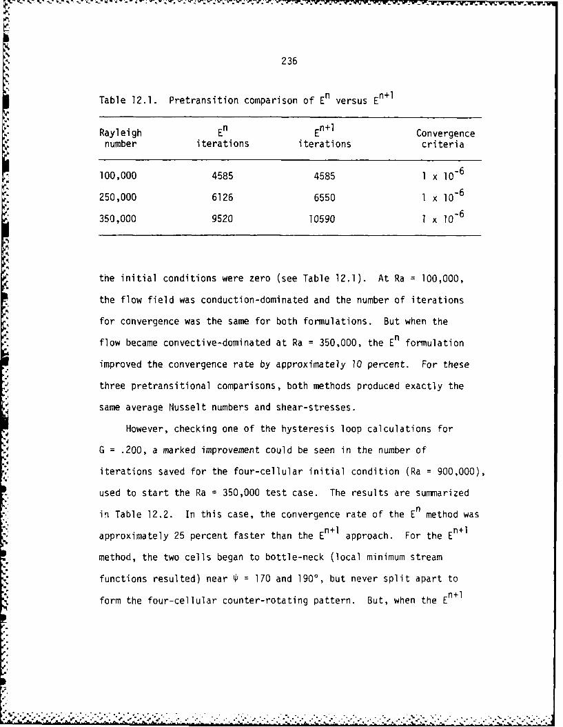
236
Table 12.1. Pretransition comparison of En versus En+1
Rayleigh En En+ 1 Convergencenumber iterations iterations criteria
100,000 4585 4585 1 x 1O6
250,000 6126 6550 1 x 1O6
350,000 9520 10590 1 x 10⁻⁶
the initial conditions were zero (see Table 12.1). At Ra = 100,000,
the flow field was conduction-dominated and the number of iterations
for convergence was the same for both formulations. But when the
flow became convective-dominated at Ra = 350,000, the En formulation
improved the convergence rate by approximately 10 percent. For these
three pretransitional comparisons, both methods produced exactly the
same average Nusselt numbers and shear-stresses.
However, checking one of the hysteresis loop calculations for
G = .200, a marked improvement could be seen in the number of
iterations saved for the four-cellular initial condition (Ra = 900,000),
used to start the Ra = 350,000 test case. The results are summarized
nin Table 12.2. In this case, the convergence rate of the E method was
approximately 25 percent faster than the En l approach. For the En+l
method, the two cells began to bottle-neck (local minimum stream
functions resulted) near J 170 and 1900, but never split apart to
form the four-cellular counter-rotating pattern. But, when the En+l
F;:.(~-

237
Table 12.2. Multicellular flow comparison of En versus En+ l
Rayleigh Iteration Convergence Cellularnumber number criteria structure
E 350,000 5850 1 x I06 4-cells
En+l 350,000 7790 1 x 1O-6 2-cells
method was repeated with a convergence constraint of 7.5 x 10 -7 , the
4-cell pattern was achieved. Therefore, it appears that as the En+l
convergence constraint is reduced, its calculations compare more
favorably to those of En for multicellular flows.
Thus, the En method has both speed and accuracy advantages when
multicellular flow is experienced. This is most probably due to
added stability, since En is always constant when iterating on flow
variable calculations for a new time-step. Also, a relaxation strategy
is not necessary when using the En formulation. For these reasons, the
En approach was used in the 2-D Navier-Stokes numerical scheme.

238
13. APPENDIX D: HEA TRANSFER AND SHEARSTRESS RELATIONS
13.1. Dimensionless Nusselt Numbers
The local heat transfer rates along the heated inner cylinder wall
and the cooled outer cylinder wall are calculated from first principles.
For the inner and outer cylinders, these local rates are given by: p.
3TS
qi -k - (13.1)
r=a
qo -k . .r (13.2)
r= b
where a, b are the radii of the inner and outer cylinders,
respectively. Using the definition of Nusselt number based on the•Kinner cylinder radius, Eqs. (13.1) and (13.2) can be nondimensionalized
to yield the following expressions:
aqi 1 3TNu = '~ (13.3) "Nui : k(Ti - To) -G r:rO (3)"
*l 0 r=.
a qo - 1 3T (13.4)
Nu0 = k(T - T0) - G Tr r=l
The average heat transfer rates can be found by simply integrating
the local radial temperature gradients along the inner and outer
cylinder walls:
'p%
.5'S.q
• .. ..-.,-.....-,.- . .-, .- .- , - . .. , . .. . . . % -. . - . - - , -. - -. . -. . • . . . . . . . .5;

239
2Nu '= T dlP (13.5)Ni : 2T-G 0 a- r:0=
= -T d P . (13.6)
U 2-rG 0 rrl
Note that when symmetry is assumed, the integrations are carried out
for only the half-annulus, or from 0 to Tr. Numerically, the integrations
of (13.5) and (13.6) are approximated by using a second-order trapezoidal
rule with variable increments, thus preserving the formal second-order
accuracy of the numerical method. Also note that since there are no
internal heat-generating sources (or sinks), the inner and outer
average Nusselt numbers should equal each other upon reaching steady
state, i.e., Nui = N-0
13.2. Dimensionless Shear Stresses
Also from first principles, the local shear stresses at the inner
and outer cylinder walls are defined as:
i : - -r(13.7)r =a
= - P(13.8)
r=b
where u is the dynamic viscosity coefficient and - is the radial
gradient of the tangential velocity component. Expressing in terms

240
of the stream function and then, nondimensionalizing yields the
following relations for the local shear stresses:
_ 1 a 2f (13.9)Yi ' G- ar- lr=O
2
Y 0 a 1 2 (13.10)YO -I G'- 3r- -lr=l
The average shear stresses can also be obtained by integrating the
local values along the inner and outer cylinders:
_ -I. - d4' (13.11)i 27rG 0 ar r=O
-1 2i2O- 1- f a f d . (13.12)
2 TG 0 ar r=l
Again, the integrations were carried out numerically by using a
second-order trapezoidal rule with variable increments.
13.3. Heat Transfer and Shear Stress Finite-DifferenceExpressions
In order to numerically approximate the local and average Nusselt
numbers as given in Eqs. (13.3) - (13.6), finite-difference expressions
for the radial temperature gradient on the inner and outer cylinder
walls must first be obtained. To do this, a second-order polynomial
curve fit was employed:
i%

241
Tn+l= an + l + bn+l Ari + c n+l Ar 2 (13.13)i~j 3 .) 1
n+lUsing the inner cylinder boundary condition, ,j = 1, the following
equations can be written:
T = an~l 1 for all j (13.14a)1,j j
Tn+l bn+l n+l Ar22,j l+ Ar2 + j 2 (13.14b)
Tn+3j I + b n+ (Ar2 Ar 3 ) + Cn+l (Ar2 + Ar3)2
(13.14c)
where Ar1 =0 and Ar. = r. - r. for i = 2, 3. Note that i 11 i-l
corresponds to the inner cylinder wall at r = 0 and i = 2, 3 represent
consecutive nodal points in the positive radial direction. Then, sincep
n+laT bn+l
ar bi~
one obtains, after some algebra, the following expression for the
inner local Nusselt number:
• n+l , _Tn+l
Nu. - 2 (13.15)G Ar2
where
7, '# € , , , ," " .. '" . .'. 5 *' ". .'_: ",' .'_' ";" . :w " ."* . ... - "r , " . .. ,,-, S." .r, r ',o .. q.. e _, ._ . ' .- , . *.. .... . .

I . k -. .
242
Tn+l Ar 2 + Ar3) Tn+l
n+l 1 + Ar 2 2,jci
~r2
(Ar +-Ar 2 22 3) ( 1 Ar2 + Ar 3
, Tn+ 1Similarly, using the outer wall boundary condition, T = 0, the
NRJ =0 h
expression for the outer local Nusselt number becomes:
T n+l ANAr + ArNR1 _ Tn+l
NRI,j (Ar NR NR TNR2,jNu0 = N N N2 (13.16)
G(Ar + A rNR + ArNR1NR ArNRl )( ArNR
where
ArNR = rNR -r NRl
Ar r - rNR1 NRl NR2
and i = NR corresponds to the outer cylinder wall at r 1, while
i = NRl, NR2 represent consecutive nodal points in the negative radial
direction.
In the same fashion, a similar polynomial fit as in Eq. (13.13),
can also be used for the stream function in order to obtain
expressions for the inner and outer local shear stresses. Employing
-1

.- .,% .. .. ._ '_ V _ 4 .. °
243
the boundary conditions
ffn+l = fn+ll,j -NR,j
Eqs. (13.9) and (13.10) can be cast into the following algebraic
representations:
-2 (fn+l Ar2 + Ar3 fn+l3,j Ar2 2,j
Ari 2( = r2 (13.17)G2 (Ar + Ar2 + Ar3 )
and
-fn+l ArNR + ArNRl fn+l-2 NR2,j - NR NRl ,j
N= . (13.18)
G G2 (ArN + )2 ArNRN ArNRl ( ArNR + ArNR1
The above relations are valid for the 2-D Navier-Stokes equations
as used in this study. However, these relations can also be used with
the finite and zero-Prandtl number boundary-layer equations by simply
substituting the appropriate related variables for temperature, stream
function and gap number. Also, since a second-degree polynomial curve
fit was used, the Nusselt number expressions are typically of second-
order accuracy for uniform increments, while the shear stress
expressions are of first-order accuracy.

244
14. APPENDIX E: TRUNCATION-ERROR STUDY
This appendix investigates the effect of truncation error on the
numerical solution to the 2-D Navier-Stokes equations. Work begins
with the comparison of first-order upwind differencing versus second-
order central differencing of the nonlinear convective terms in the
2-D Navier-Stokes equations. Then, a mesh resolution study for three
different size gap widths is conducted to gain an idea of the uncertainty
involved in the numerically predicted transitional Rayleigh numbers of
Section 6.1. Lastly, two correlations for the mean Nusselt number are
compared to related numerical results with respect to an annulus of
diameter ratio 1.200.
14.1. Upwind Versus Central - Differencing
In Figure 14.1, the two different schemes are compared for a
pretransitional Rayleigh number of 300,000. The complete annulus was
considered with G = .200 and a mesh size of 31 x 102 nodes. The
upwind scheme was employed by setting the correction term (En) to zero
in Eq. (5.6g). The first-order upwind method compared rather well to
the central-differencing scheme in this case, with maximum relative
errors of 2-3 percent occurring near = 1800 and $ = 00, respectively.
Hence, for the pretransitional cases, the first-order upwind-
differencing method should yield fairly accurate numerical results.
However, for Ra = 1,000,000 (well beyond the point of multicellular
transition as predicted with the central-differencing scheme), the

245
00
0
co
C30
00
0ocC)
- .4.
LOL
(no
o CC)
0 &0
CU S-
4- CU4- 4- 41 D
4- -04-- 4
M, >
C3- C-
0 0
I CD
O0l O1 00*1 09*0 09*0
(Y NN I) flNU-

246
first-order upwind method was not able to resolve the multicellular
flow field, as indicated in Figure 14.2. This was most likely due to
artificial viscosity effects associated with first-order upwind-
differencing schemes. Thus, it appears that at least second-order
accuracy is needed to capture multicellular flow transition.
14.2. Mesh Resolution Study
This study examines three different gap widths with a mesh of
31 x 102 nodes for both the complete and half-annulus. Thus, the
number of angular nodes in the half-annulus is approximately doubled
compared to that in the full-annulus.
For the half-annulus, vertical center-line symmetry was assumed.
This assumption was proven valid by the symmetric multicellular flow
patterns shown in Figures 6.3c and 6.5 for G = .200 and .100,
respectively. In Figure 14.3, the angular variation of the inner-wall
vorticity is plotted for the full and half-annulus at Ra = 2,500,000
and G = .100. The results of the half-annulus mesh are nearly
identical to those of the full-annulus, within one percent relative
error for this pretransitional case. These results provide confidence
that the half-annular calculations are indeed valid.
Considering the above symmetry discussion, the following study
was performed (note: the convergence constraint was 1 x 10⁻⁶ for all
test cases shown below in Table 14.1).
Based on the results of this table, it appears that the numerically
predicted transitional Rayleigh numbers (associated with the full-annulus
N !

247
o0C)
o
oo
.. )
CD
CDC
4-)
-O.
-/ -
o ,oEV
c\Ju
// °~C3'.0
w ,-) -M
== 00
S- II
SI II0'
0W O ' 0 "I0 " 00"0
I -a N I] n
C.)C)
C33
S,
u a) CT"
0< C",
0I
4-)
4-
C3 0 L.%
',_
c
4,. "" " -" " "," """ " "'" "-" " " " "'- .,,'..'w" .% ." ," " " - " - - .. .- ... - ."4,., ._ .. ... ' . .. . . .. _ .. -. -; ; " . .. . .. - _- ... -.4*-. . .4- 4-") ; .. ... (0. ." -,, ,"

%k
248
C)
o o
CD
C)C
-~ r- c
00~-
Io ClLU
<? C
CD
00*2c~~~~~. -0*io0*101 G 0c
OLX)AiDI 0A IVM-3NN

249
Table 14.1. Mesh resolution comparison
G Mesh Geometry RaTR Rab-a Percentsize relative
error
.100 31 x 102 full-annulus 2,840,000 2840}4.4
.100 31 x 102 half-annulus 2,720,000 2720
.150 31 x 102 full-annulus 810,000 2730}7.7
.150 31 x 102 half-annulus 751,000 2535
.200 31 x 102 full-annulus 350,000 2800}14.75
.200 31 x 102 half-annulus 305,000 2440
mesh) are within 5-15 percent uncertainty. This uncertainty tends to
decrease with decreasing gap size. In addition, the transitional
Rayleigh numbers predicted with the half-annulus mesh (used mostly
in generating the small-gap stability curve of Figure 6.12) are
probably within five percent uncertainty.
It should also be noted that when a 21 x 48 full-annulus mesh
was used for G = .100 and .200, the transition to multicells did not
occur. Therefore, the ability to capture multicellular flow transition
appears to be very sensitive to first-order upwind-differencing and
mesh coarseness.
fk - -.- e_ -. . . -

250
14.3. Mean Nusselt Number Correlations
In this section, two correlations for the mean Nusselt number are
compared to this study's pretransitional numerical results for G = .200
and Pr = .706, with a full-annulus mesh of 31 x 102 node. The
empirical correlations used are those of Raithby and Hollands (1975)
and Kuehn and Goldstein (1980b), outlined in Eqs. (2.14) and (2.19),
respectively.
In Figure 14.4, the above two correlations were used to obtain mean
Nusselt numbers within 2.5 percent relative error of those obtained
numerically - for a range of Rayleigh numbers between 275,000 and
350,000. This comparison is fairly good, considering these
correlations are fitted to within 10-15 percent uncertainty of the
experimental data.
A much more convincing measure of the accuracy of the numerical
method was given in Section 6.1. There, it was shown that 2-D Navier-
Stokes pretransitional numerical results (of local flow variables)
converged to related analytical perturbation results in the limit as
G - 0 and Ra . Note that local flow variable data for narrow gap
widths could not be found in the literature, hence reinforcing the
importance of a valid analytical solution comparison.
• ° .. . . • .
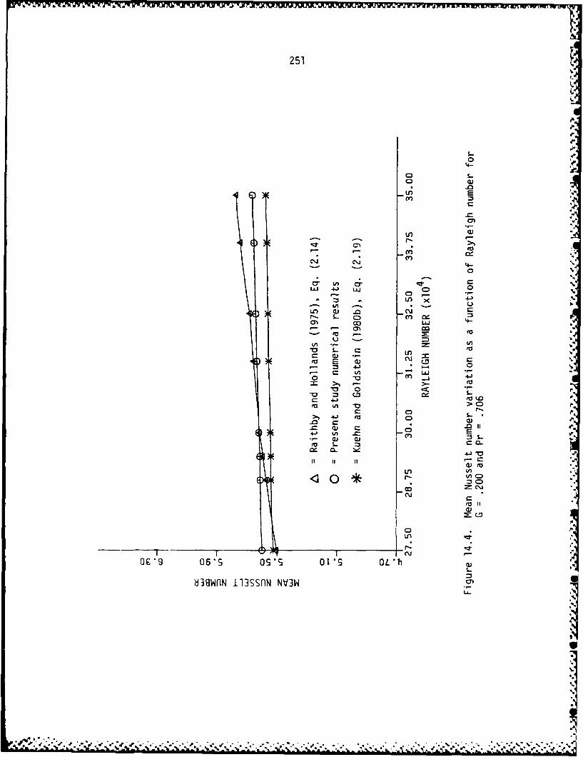
251
4-
0o
In
C),
- - 4-.
LUJ 4J LUj 0
4.*LI) x< .4-J %
fl- S- C)ao) 00 Lf) 4
,a 0-(
= >, >-(-~ 0
r_ 4j ut.0 e
>1 4.3 Vo C) '
a= CD E
S4-) A n:3S
cu o)
Lr))
0 Cru =C
cm a.
*c '9 0 6 S aos.*s 01* *s L* ~ * *..* *

- - - - .. .- ~. -
.. 4. I
V-4'.4.
4/.444
.4'I .4-
.4
.4~.
I.'-.
4% 4*4~
4%
4.4I.
'4$
.4.-
4%*44
... 4
'g~.4I-
4".'Sb
4$(.4.-~ ~4.
'.4Id
.4.4.
.~.4
*~~~$* ,.~..44
.4$%..4\.4,p.. . . * .4.4.4.4.... *.44$ ~.44$