1

Mumford–Shah Model for One-to-one EdgeMatching

Jingfeng Han∗, Benjamin Berkels, Marc Droske, Joachim Hornegger, Member, IEEE,Martin Rumpf, Carlo Schaller, Jasmin Scorzin and Horst Urbach

Abstract—This paper presents a new algorithm based on theMumford–Shah model for simultaneously detecting the edgefeatures of two images and jointly estimating a consistent set oftransformations to match them. Compared the current asymmet-ric methods in the literature, this fully symmetric method allowsone to determine one-to-one correspondences between the edgefeatures of two images. The entire variational model is realizedin a multi-scale framework of the Finite Element approximation.The optimization process is guided by an EM type algorithmand an adaptive generalized gradient flow to guarantee a fast andsmooth relaxation. The algorithm is tested on T1 and T2 magneticresonance image (MRI) data to study the parameter setting. Wealso present promising results of four applications of the proposedalgorithm: inter-object mono-modal registration, retinal imageregistration, matching digital photographs of neurosurgery withits volume data and motion estimation for frame interpolation.

Index Terms—Image registration, edge detection, Mumford–Shah model

I. INTRODUCTION

IN 1989 the general Mumford–Shah model [1] was firstproposed in the literature. In this model, an image is

approximated by a cartoon (u,K): u is a piecewise smoothimage with sharp edges and K is the discontinuity set inthe image domain. This model has been extensively studiedfor segmentation, image denoising and shape modelling, seei.e. [2], [3], [4], [5] and the references therein.

In 2005 Droske et. al [6], [7] expanded the Mumford–Shah model with the capability of matching the edge featuresof two images. The edge features are represented by twodifferent cartoon approximations of the images. A smoothdense warping function defines the mapping between theedge features. The modified Mumford–Shah model seeks tosimultaneously tackle two highly interdependent tasks: edgesegmentation and non-rigid registration. An important benefitof such a joint model is that the intermediate results of onetask serve as prior knowledge to the solution of the othertask. This advantage has already been pointed out by Yezzi,Zollei and Kapur [8], who simultaneously segmented edges indifferent images based on affine matching deformations and

Manuscript received January 8, 2007; revised May 2, 2007. The work issupported by Deutsche Forschungsgemeinschaft (DFG) under the grant SFB603, TP C10. The Associate Editors responsible for coordinating the review ofthis paper and recommending its publication was T. Aach. Asterisk indicatescorresponding author.∗J. Han and J. Hornegger are with the Chair for Pattern Recognition,

University of Erlangen-Nurnburg, Germany. B. Berkels, M. Droske and M.Rumpf are with the Institute for Numerical Simulation, University of Bonn,Germany. C. Schaller, J. Scorzin and H. Urbach are with the Department ofNeurosurgery, University of Bonn, Germany.

Fig. 1. Non-symmetric Mumford–Shah model for edge matching. R0

and T0 are the given reference and template images. R and T are therestored, piecewise smooth functions of image R0 and image T0. K is thecombined discontinuity set of both images. Function Φ represents the spatialtransformation from image T to image R.

an active edge model for the segmentation of implicit curvesand surfaces in images, similar to the one proposed by Veseand Chan [9].

A major drawback of the above Mumford Shah basedmatching is its asymmetry with respect to edge features andthe spatial mapping between them. The scheme of the modelis shown in Fig. 1. The definition of the similarity measure isnot symmetrical: a joint discontinuity set K is used to estimatethe edges of the restored template image T and the deformededges of the restored reference image R. The model of thespatial mapping between the two images is not symmetrical:the transformation Φ in Fig. 1 is only defined in one direction,from the image T0 to the image R0. The asymmetry of thesimilarity measure and the single directional transformation, aspointed out in [10], cannot ensure that the method is consistent,i.e., if one uses it to compute the transformation Φ from T0

to R0 and then switches the roles of T0 and R0 to computethe transformation Ψ from R0 to T0, it is uncertain whetherthese transformations are inverse to each other.

In this paper we propose a new symmetric model for edgematching again based on the Mumford–Shah model. Fig. 2shows the scheme of this symmetric model. We use tworelatively separated discontinuity sets (KR and KT in Fig. 2)to explicitly represent the edge sets of the associated images.For the ambiguity problem of the correspondence, we applythe idea of consistent registration [11], [12] to simultaneouslyestimate the forward and reverse transformations and to con-strain one transformation to be the inverse of the other one.

2

Fig. 2. Symmetric Mumford–Shah model for one-to-one edge matching. R0

and T0 are the given images. R and T are the restored, piecewise smoothfunctions of image R0 and image T0. KR and KT are the discontinuity setsof the images R and T , respectively. Function Φ represents the transformationfrom image T to image R and function Ψ represents the transformation fromimage R to image T .

In this way, the edge sets KR and KT of the images R andT , respectively, have equal influence on the edge registration.Thus, the proposed method is one-to-one in the sense, that itallows to determine one-to-one correspondences between theedge features of two images.

Symmetric one-to-one edge matching is not only moresound in the mathematical sense, but also very significantin a broad range of applications, where one is interestedin determining the correspondence of the same structure indifferent images (e.g., non-rigid registration for atlas con-struction [13], [14], historical biological images [15], [16] ormotion estimation).

The paper is organized as follows: In Section II, we in-troduce some basic knowledge about the classic Mumford–Shah model, the approximation proposed by Ambrosio andTortorelli and the Finite Element approximation as a prepa-ration for the discussion of the proposed method. After-wards, in Section III we present the method of one-to-oneedge matching, including the functional definitions, variationalformulations, numerical implementations and algorithm. InSection IV, we study the parameter setting of the algorithmand show experimental results for several applications. Finally,we draw conclusions in Section V. We note that a preliminaryversion of part of the work reported in this article has appearedin our conference paper [17].

II. BACKGROUND

A. Mumford–Shah Model

For a function u0 : Ω → R on an image domain Ω ⊂ Rd

with d = 2 or 3 and nonnegative constants α, β and ν, theMumford–Shah (MS) functional is given by

EMS(u,K) =α

2

∫

Ω

(u− u0)2

+β

2

∫

Ω\K|∇u|2 dx +

ν

2Hd−1(K).

(1)

The first term measures the degree of fidelity of the approxi-mation u with respect to the input data u0. The second term

acts as a kind of “edge-preserving smoother”, which penalizeslarge gradients of u in the homogeneous regions while notsmoothing the image in the edge set. The last term Hd−1

denotes the d − 1 dimensional Hausdorff measure, which isused to control the length of the edge set.

B. Ambrosio–Tortorelli Approximation

It is difficult to minimize the original Mumford–Shah func-tional (1) because of its implicit definition of the discontinuityset K. Various approximations have been proposed during thelast two decades. In this article we focus on the Ambrosio–Tortorelli approximation with elliptic functionals [18].

In the Ambrosio–Tortorelli (AT) approximation the discon-tinuity set K is expressed by a phase-field function v. Thisscalar function v approximates the characteristic function ofthe complement of K, (1− χK), i.e., v(x) ≈ 0 if x ∈ K andv(x) ≈ 1 otherwise. The entire approximation functional isdefined as follows:

EεAT[u, v] =

α

2

∫

Ω

(u− u0)2 dx +β

2

∫

Ω

v2‖∇u‖2 dx

+ν

2

∫

Ω

(ε‖∇v‖2 +14ε

(v − 1)2) dx,

(2)

The second term, still working as an “edge-preservingsmoother”, couples zero-regions of v with regions where thegradient of u is large. The following “coupling” between uand v is energetically preferable:

v(x) ≈ 0 where ‖∇u‖ À 0,≈ 1 where ‖∇u‖ ≈ 0.

(3)

The last term approximates the edge length, i. e. the d − 1dimensional measure Hd−1(K) of the edge set K. Theparameter ε controls the “width” of the diffusive edge set.Mathematically speaking, the sequence of functionals Eε

ATΓ−converges to the Mumford–Shah functional, i.e.

Γ− limε→0

EεAT = EMS.

For a rigorous proof and further explanation we refer to [19].

C. Finite element method

Finite Element (FE) methods are used in this work todiscretize the equations. The whole image domain Ω is coveredby an uniform rectangular mesh C, on which a standard multi-linear Lagrange finite element space is defined. We considerall images as sets of voxels, where each voxel corresponds toa grid node of C. Let N = x1, ..., xn denote the nodes of C.The FE basis function of node xi is defined as the piecewisemulti-linear function that fulfills:

ϕi(xj) =

1 i = j

0 i 6= j.

The FE-space V is the linear hull of the ϕi, i.e.

V := span(ϕ1, ..., ϕn).

The FE-space of vector valued functions is Vd, the canonicalbasis of this space, is

ϕ1e1, ..., ϕne1, ..., ϕ1ed, ..., ϕned,

3

where ei is the i-th canonical basis vector of Rd. In the FE-space scalar and vector valued functions, e.g. U and Φ, areapproximated as follows:

U ≈ U :=n∑

i=1

U(xi)ϕi(x) and

Φ =

Φ1

...Φd

≈ Φ :=

∑ni=1 Φ1(xi)ϕi(x)

...∑ni=1 Φd(xi)ϕi(x)

.

The FE approximation of a function can also be representedby the vector of the function values on the nodes, e.g.U := (U(xi), · · · ,U(xn))T and Φ := (Φ1, · · · ,Φd)T whereΦj = (Φj(x1), · · · ,Φj(xn))T . In this paper we denotecontinuous functions by uppercase letters (e.g. U or Φ), theirFE representation by boldface uppercase letters (e.g. U orΦ) and their vector representation by “over-lined” uppercaseletters (e.g. U or Φ).

III. ONE-TO-ONE EDGE MATCHING

A. Problem Statement

The major task of image registration is stated as follows:Find an appropriate transformation Φ such that the transformedtemplate image T0 Φ becomes similar to the reference imageR0 [20]. The degree of similarity (or dissimilarity) is evaluatedusing the gray values R0 and T0 or certain features such asedges. We consider a edge based matching method that seeksto register two images based on a joint edge extraction andregistration. Thus, the algorithm simultaneously has to fulfillthe two following tasks:

• Detection of the edge features from two noisy images.• Registration of two images using these detected edge

features.

The first task is more related to image denoising and edgedetection, for which we simply employ the Mumford–Shahmodel as the feature representation. In practice, the discon-tinuity sets are approximated by phase-field functions as inthe Ambrosio–Tortorelli approximation. Thus, four unknownsR, T, V, W are estimated, where (R, V ) and (T,W ) are thefeature representations of R0 and T0, respectively.

The second task is more related to image registration.The non-rigid transformation from image R0 to image T0 isfrequently different from the inverse function of the trans-formation from T0 to R0. In order to overcome such cor-respondence ambiguities, we follow the method of consistentregistration [11] to jointly estimate the transformations in bothforward and reverse directions. We denote the transformationfrom T0 to R0 as Φ and the transformation from R0 to T0 as Ψ.Functions Φ and Ψ are estimated to match the two feature rep-resentations (R, V ) and (T, W ) to each other. Additionally, Φand Ψ are required to be smooth and approximately inverse toeach other. For the desired spatial properties, a regularizationfunctional and a consistency functional are used to constrainthe transformations to satisfy these requirements.

B. Functional Definitions

The six unknowns - the restored reference image R, therestored template image T , the edge describing phase-fields Vand W of the reference and the template image, respectively,and the deformations Φ and Ψ from the template to thereference domain and vice versa - are estimated by minimizinga joint functional with the following structure:

ESYM = EAC + µECC + λEREG + κECON, (4)

where µ, λ and κ are nonnegative constants which controlthe contributions of the associated functionals. The detaileddefinitions of these functionals are as follows:

1) Auto-coupling Functional:

EAC =CAC[R, V ] + CAC[T,W ]:=Eε

AT[R, V ] + EεAT[T, W ].

(5)

Here EεAT denotes the functional of the Ambrosio–Tortorelli

approximation whose definition has been given in equation (2),where u0 is replaced by R0 or T0 respectively. The singleauto-coupling cost function, e.g., CAC[R, V ], essentially makesuse of the mechanisms of the Mumford–Shah model andits Ambrosio–Tortorelli approximation to estimate the featurerepresentation (R, V ) of the image R0, such that the piecewisesmooth function R optimally couples with the phase-fieldfunction V in a manner similar to equation (3). Roughlyspeaking, this auto-coupling functional is responsible for de-tecting the edge features of each image and for definingthe internal relation between the phase-field function V (orW respectively) and the piecewise smooth function R (or Trespectively). In this functional the segmented edge featuresof the two images, i.e. (R, V ) and (T, W ), are totally inde-pendent from each other.

2) Cross-coupling Functional:

ECC =CCC[R,W,Φ] + CCC[T, V,Ψ]

:=12

∫

Ω

(W Φ)2 ‖∇R‖2 dx

+12

∫

Ω

(V Ψ)2 ‖∇T‖2 dx.

(6)

This functional is responsible for matching the edge featuresof the two images. It favors spatial transformations Φ and Ψwhich optimally couple the feature representations (R, V ) and(T,W ) in the following way:

W Φ ≈

0 where ‖∇R‖ À 0,1 where ‖∇R‖ ≈ 0.

V Ψ ≈

0 where ‖∇T‖ À 0,1 where ‖∇T‖ ≈ 0.

By definition, this functional jointly treats segmentation andregistration: For the registration, the functional can act asthe similarity measure based on the intermediately segmentededge features. Instead of directly matching the phase-fieldsfunctions (V ↔ W ) and the smooth functions (R ↔ T ),the functional seeks to match the gradient field of the smoothfunction of one image to the phase-field function of the otherimage (V ↔ ∇T,W ↔ ∇R). For the segmentation, thisfunctional also imposes the influence of the edge features

4

segmented in the other image. In the following subsectionwe will see that both spatial transformations are controlledby regularization. The regularized spatial transformations leadto local edge feature correspondence.

3) Regularization Functional:

EREG =CREG[Φ] + CREG[Ψ]

:=12

∫

Ω

‖D(Φ− 11)‖2 dx

+12

∫

Ω

‖D(Ψ− 11)‖2 dx.

(7)

Here 11 : x 7→ x denotes the identity mapping and Φ − 11,Ψ − 11 the displacement fields corresponding to Φ and Ψ.Generally speaking, the regularization functional is used torule out singular transformations which may lead to cracks,foldings, or other undesired properties. In this work theregularization constraint is the sum of the norm of the Jacobianof both displacement fields (see [21] for further explanationsof regularization based on the Jacobians of transformations).

Other candidates for regularization constraints are linearelastic [22], [23] and viscous fluid [24], [23] regularizations.These two constraints make use of the continous mechanicalmodel to regularize the transformations [25]. Another alterna-tive, which already ensures a homeomorphism property, is thenonlinear elastic regularization which separately cares aboutlength, area and volume deformation and especially penalizesvolume shrinkage [26].

4) Consistency Functional:

ECON =CCON[Φ, Ψ] + CCON[Ψ, Φ]

:=12

∫

Ω

‖Φ Ψ(x)− x‖2 dx

+12

∫

Ω

‖Ψ Φ(x)− x‖2 dx.

(8)

The forward and reverse transformations Φ and Ψ are purelyindependent of each other in EAC and EREG and are implicitlycorrelated in ECC via the matching of the two image / phase-fields pairs, i.e. (R, W Φ) ↔ (T, V Ψ). The consistencyfunctional ECON in equation (8) explicitly specifies the rela-tionship between forward and reverse transformations: ECCis minimal if and only if Φ Ψ(x) = x = Ψ Φ(x),i.e., Φ ≈ Ψ−1 and Ψ ≈ Φ−1. The transformation in onedirection has to be the inverse function of the transformationin the other direction. For the registration, this consistencyconstraint favors an invertible and bijective correspondence ofthe segmented edge features.

C. Variational Formulation

We assume that the minimum of the entire energy ESYMis the zero crossing of its variation with respect to all theunknowns R, T, V, W,Φ, Ψ. The definition of the entirefunctional ESYM, as well as each individual functional EAC,ECC, EREG and ECON, is symmetric with respect to thetwo groups of unknowns: R, V, Φ and T, W,Ψ. Thus,we restrict ourself to the description of the computation ofvariations with respect to R, V, Φ. The variational formulasof the other group can be deduced in a complementary way.

Given an arbitrary scalar test function ϑ ∈ C∞0 (Ω), weobtain the variations with respect to R and V :

〈∂RESYM, ϑ〉 = 〈∂REAT, ϑ〉+ 〈∂RECC, ϑ〉=

∫

Ω

α(R−R0)ϑ + βV 2∇R · ∇ϑ dx

+∫

Ω

µ(W Φ)2∇R · ∇ϑ dx,

(9)

〈∂V ESYM, ϑ〉 = 〈∂V EAT, ϑ〉+ 〈∂V ECC, ϑ〉=

∫

Ω

β ‖∇R‖2 V ϑ +ν

4ε(V − 1)ϑ dx

+∫

Ω

νε∇V · ∇ϑ dx

+∫

Ω

µ‖∇T Ψ−1‖2V ϑ |detDΨ|−1 dx.

(10)

Here we have used the transformation rule∫

Ω

µ

2‖∇T‖2V 2 Ψdx

=∫

Ψ(Ω)

µ

2‖∇T Ψ−1‖2V 2 |det DΨ|−1 dx

and Ψ(Ω) = Ω. Given an arbitrary vector-valued test functionζ ∈ C∞0 (Ω,Rd), we obtain the variation with respect to Φ:

〈∂ΦESYM, ζ〉 = 〈∂ΦECC, ζ〉+ 〈∂ΦEREG, ζ〉+ 〈∂ΦECON, ζ〉=

∫

Ω

µ ‖∇R‖2 (W Φ)∇(W Φ) · ζ dx

+∫

Ω

λDΦ : Dζ dx

+∫

Ω

κ([Φ Ψ](x)− x) · [ζ Ψ](x) dx

+∫

Ω

κ([Ψ Φ](x)− x)DΨ(Φ(x)) · ζ(x) dx.

(11)

Due to the high complexity of the minimization prob-lem (four scalar functions and two vector-valued functions)the unknowns are estimated in an Estimation-Minimizationlike (EM) procedure: Let fi=1,...,m denote the unknownfunctions and E := E[f1, ..., fm] denote the functional.

while fi=1,...,m has not yet converged dofor i = 1 to m do

fi = arg minf E[f1, ..., fi−1, f, fi+1, ..., fm].end for

end while

D. Solution of the linear part

First we introduce generalized mass and stiffness matrices,which play the key roles in the discretization of equations (9)and (10) using FE approximation.

5

Given a function f(x) : Ω 7→ R, the generalized mass M [f ]and stiffness matrices L[f ] are defined as follows:

M [f ] =(∫

Ω

f(x)ϕi(x)ϕj(x) dx

)

i,j

(12)

L[f ] =(∫

Ω

f(x)∇ϕi(x) · ∇ϕj(x) dx

)

i,j

(13)

Both matrices are n× n-dimensional, where n is the numberof nodes in the FE space. Both matrices are sparse, i.e. mostentries are zero. An entry is non-zero, if and only if i = jor node i and j are adjacent in the mesh. To compute theintegrals in these non-zero entries we use a numerical Gaussianquadrature scheme of order three (cf. [27]). Obviously, thecommon mass matrix M and stiffness matrix L are just specialcases of the generalized ones, i.e. M := M [1] and L := L[1].

The variations in equation (9) and (10) are linear with re-spect to the unknowns R and V respectively. In each iterationof the EM procedure, the zero-crossings are simply calculatedby solving the corresponding linear systems. Replacing thecontinuous functions R0 and R with their FE approximationsR0(x) =

∑ni=1 Ri

0ϕi(x) and R(x) =∑n

i=1 Riϕi(x) andconsidering base functions ϕj of the FE space as test functions,the equation for zero crossings of (9) is equivalent to:

α

n∑

i=1

n∑

j=1

Ri

∫

Ω

ϕi(x)ϕj(x) dx

+ β

n∑

i=1

n∑

j=1

Ri

∫

Ω

V2(x)∇ϕi(x) · ∇ϕj(x) dx

+ µ

n∑

i=1

n∑

j=1

Ri

∫

Ω

(W Φ)2(x)∇ϕi(x) · ∇ϕj(x) dx

= α

n∑

i=1

n∑

j=1

Ri0

∫

Ω

ϕi(x)ϕj(x) dx

(14)

Using the notations of generalized mass (12) and stiffnessmatrices (13), equation (14) can be rewritten as:

(αM + βL

[V2

]+ µL

[(W Φ)2

])R = αMR0. (15)

Similarly (10) leads to:(

µM[‖∇T Ψ−1‖2 |detDΨ|−1

]

+βM[‖∇R‖2

]+

ν

4εM + νεL

)V =

ν

4εM1.

(16)

Here 1 denotes the one-vector, i.e. (1, · · · , 1)T . Analogously,we get the linear systems for T and W :

(αM + βL

[W2

]+ µL

[(V Φ)2

])UT = αMT0. (17)

(µM

[‖∇R Ψ−1‖2 |det DΨ|−1

]

+βM[‖∇T‖2

]+

ν

4εM + νεL

)VT =

ν

4εM1.

(18)

The linear systems (15) - (18) are solved with a preconditionedConjugate-Gradient (CG) method.

E. Solution of the nonlinear part

Equation (11) shows that the variation of the energy isnonlinear with respect to one of the transformations. Thusthe unknown transformation cannot be estimated by solvinga linear system. Instead we employ a regularized gradientdescent method to iteratively find the zero-crossing:

Φk+1 = Φk − τk · gradgσ

Φ E[Φk], (19)

where gradgσ

Φ E[Φk] is the regularized gradient with respect tothe unknown Φ and a metric gσ, and τk is the step size.

1) gradgσ

Φ E[Φk]: This regularized gradient combined withthe time discretization is closely related to iterative Tikhonovregularization, which leads to smooth paths from the initialdeformations towards the set of minimizers of the matchingenergy. As metric we choose:

gσ(Φ1,Φ2) = (Φ1,Φ2)L2 +σ2

2(DΦ1, DΦ2)L2 .

For theoretical details, we refer to [28], [29], [30]. In ourimplementation, the regularized gradient gradgσ

Φ E[Φk] is com-puted in two steps:• Compute the variation

∂ΦE[Φk] =⟨∂ΦESYM[Φk], ζ

⟩

according to equation (11), where the integrals are com-puted with a Gaussian quadrature scheme of order threeand the test functions are the canonical basis functionsof Vd, see Section II-C.

• The representation of the metric in FE-terms is

gσ(Φ1,Φ2) =(Mbl. + σ2

2 Lbl.

)Φ1 · Φ2

which leads to

gradgσ

Φ E[Φk] =(Mbl. + σ2

2 Lbl.

)−1 (∂ΦiE[Φk]

)i.

Here Mbl. and Lbl. denote d× d block matrices with thestandard mass and stiffness matrices respectively on thediagonal positions, and zero matrices on the off diagonalpositions. We use σ =

√10h, where h is the mesh

resolution. The solution of the linear system is computedby a single V -cycle of a multigrid solver.

At this point, we see that the principle difference from“classical” gradient descent methods is that the regularizedmethod does not use the primitive variation but a regularized(smoothed) one as descent direction.

2) τk: The step size of the gradient flow is determinedby the Armijo-rule[31], choosing the largest τk such thatenergy is minimized in a successive reduction rule. Thenatural way in the EM procedure is to estimate the step sizefor each transformation individually, i.e. estimating τΦ forthe transformation Φ then estimating τΨ for Ψ. However,if τΦ and τΨ are estimated sequentialy in each iteration,the consistency functional in (6) will prevent τΦ and τΨfrom being large, because large individual step sizes willincrease the consistency functional significantly. Consequently,the regularized gradient descent requires a large number ofiterations to approach the minimum. In order to solve this

6

Fig. 3. A simple 2-d example of nested mesh hierarchy. The nodes of thecoarse mesh C1 are a subset of the nodes of the fine mesh C2. The prolongationof a function from the mesh C1 to the mesh C2 only requires the interpolationof the function values on the new nodes.

problem, we simultaneously estimate both transformations andcompute one step size for both of them:

[Φk+1

Ψk+1

]=

[Φk

Ψk

]− τk

[gradgσ

Φ E[Φk,Ψk]gradgσ

Ψ E[Φk,Ψk]

]. (20)

Since Φ and Ψ are updated at the same time, the consistencyenergy does not penalize a large step size τk any more.

Let Θ := [Φ,Ψ]T , gradE[Θ] := [gradgσ

Φ E, gradgσ

Ψ E]T andE′[Θ] := [E

′[Φ], E

′[Ψ]]T . We define the condition for the

Successive Reduction Rule (SRR) as:

EREG[Θk − τk · gradE[Θk]]− EREG[Θk]〈E′ [Θk], gradE[Θk]〉 >

14.

The step size τk is estimated as follows:

% Initialize τk from previous iteration.if k = 0 then τk = 1.0else τk = τk−1

% Find the largest τk fulfilling SSR.if SSR succeeds then

do τk = 2τk until SSR failselse

do τk = 0.5τk until SSR succeedsend if

The regularization of the gradient and the adaptive estimationof the step size allow the regularized gradient descent methodto perform more efficiently than the classical ones. In mostcases we use five gradient descent steps to estimate thetransformations in each iteration of the EM procedure.

F. Multi-scale Algorithm

In order to avoid being trapped in local minima, the algo-rithm employs a spatial multi-scale scheme, in which globalstructures are segmented and matched before local ones.

The image domain Ω := [0, 1]d is discretized by a rec-tangular mesh Cm, which has 2m + 1 equidistant nodes ineach axis, thus n := (2m + 1)d nodes total. m is called thelevel of the mesh. A discrete function on the mesh Cm canalso be called a function on level m. Fig. 3 shows a 2-dexample of two nested meshes C1 and C2, in which the featurerepresentations R, V, T, W and the transformations Φ, Ψare first computed on the coarse mesh C1. Then the results areprolongated to the next higher level on the finer mesh C2.

Although such a nested mesh hierarchy is not natural forfinite difference methods, where commonly discrete imageswith 2m voxels in each axis are used, it is common for thecanonical hierarchy in the Finite Element context. This waythe prolongation from one level to the next higher level isvery convenient. Let Nm denote the set of nodes of the m-thmesh, as shown in Fig. 3. The nested mesh hierarchy ensuresNm−1 ⊂ Nm. During prolongation from level m−1 to m thefunction values stay the same on the nodes in Nm−1 and thefunction values on the nodes in Nm\Nm−1 are determined bymulti-linear interpolation from the values on the neighboringnodes in Nm−1.

The entire multi-scale algorithm is summarized as follows:

given images R0 and T0.given starting level m0 and ending level m1.given number of iterations on each level k1.intialize [Rm0 ,Vm0 ,Tm0 ,Wm0 ] with 0.intialize [Φm0 ,Ψm0 ] with 11.for m = m0 to m1 do

for k = 1 to k1 doupdate Rm through equation (15)update Vm through equation (16)update Tm through equation (17)update Wm through equation (18)update [Φm,Ψm] with 5 regularized gradient descent stepsthrough equation (20)

end forif m 6= m1 then

intialize [Rm+1,Vm+1,Tm+1,Wm+1,Φm+1,Ψm+1]through prolongation from [Rm,Vm,Tm,Wm,Φm, Ψm]

end ifend for

IV. RESULTS

Five experiments are performed to demonstrate the one-to-one edge matching algorithm. The first one is designed tostudy the parameter settings of the algorithm. We have chosenT1- and T2-MRI volumes of the same patient as input data.The second one is designed to show the effect of the algorithmin 3-d inter-object monomodal registrations, whose major taskis to build up anatomical correspondence between differentindividuals. The third experiment shows the application of thealgorithm in the registration of retinal images. Then we presentresults of matching 2-d photographs taken during neurosurgeryto the projections of 3-d MRI volume data. Finally we showthat the method can be used in the application of frameinterpolation. In order to comply with the mesh hierarchyintroduced in section III.F, the data sets in experiments A,B, C and D are resampled, while the data set in experimentE is cropped. We have chosen multi-linear interpolation, i.e.bilinear for 2-d data and trilinear for 3-d data, because itconveniently fits into our Finite Element framework and givesacceptable accuracy. But the method does not depend on theway the data is resampled nor on the concrete construction ofa multi-scale.

A. Parameter study for 3-d data

Two MRI volumes are acquired from the same individualand with the same machine but with the different scan pa-

7

T1 T2

V1 V2

A1

β = 7.92

µ = 0.08

λ = 1000

A2

β = 0.08

µ = 7.92

λ = 1000

A3

β = 4

µ = 4

λ = 1000

A4

β = 4

µ = 4

λ = 10

Fig. 4. Experiments A1-A4 show the influence of the parameters β, µ and λon the phase-field functions. In experiments A1-A3, the overwhelmingly largeλ disables the edge matching functionality and allows only edge detections.Furthermore, the ratio between β and µ determines whether the phase-fieldsrepresent edge features of its own image or the features of its counterpart. Inexperiment A4 edge matching as well as edge detection are enabled. Note thatedge matching merged the phase-fields of both sides compared to experimentA3.

rameters (T1/T2). The original T1-MRI (our reference imageR0) and T2-MRI (our template image T0) volumes are alreadynearly perfectly matched to each other. In order to demonstratethe effect of registration, the T2-MRI volume is artificiallydeformed by a given elastic transformation. We specifiedthe displacement vectors on eight points and computed thedisplacement vectors in the remaining part of the data usingthin-plate spline interpolation. Both of the given volumesare of size 512 × 512 × 101 and have been resampled to129 × 129 × 129 pixels to comply with the mesh hierarchypresented before. We performed 18 experiments with differentparameter settings. For each experiment 10 EM-iterations wererun on the 129× 129× 129 mesh. It took approximately twohours for each experiment on a standard PC with Intel Pentium4 processor 2.26 GHz and 2.0 GB RAM. It is expected thatthe computational time will decrease significantly by furtheroptimization of the code. Although these parameters are onlytested for T1-/T2-MRI edge matching, they can also be usedto determine the parameters for edge matching of the othermodalities.

Experiments A1-A4 demonstrate how the parameters β, µand λ balance the edge detection and the edge matching inthe algorithm. The other parameters are fixed at α = 2550,ν = 0.1, κ = 100, ε = 0.01. In this example, we denotethe phase field functions of T1- and T2-MRI volumes as V1

and V2 respectively. Fig. 4 shows how the two phase-fieldfunctions varied in a local region with different parameters. Inthe experiments A1-A3, the overwhelmingly large regulariza-tion weighting parameter λ (= 1000) prevents the algorithmfrom matching the edge features of the two images. Withoutconsideration of the edge matching, the detection of edgefeatures is controlled by the ratio between the auto-couplingweighting parameter β and the cross-coupling weighting pa-rameter µ. In experiment A1, since β is much larger thanµ, the auto-coupling functional EAC has more influence thanthe cross-coupling functional ECC. The resulting phase-fieldfunctions are more likely to describe its own edge feature.Experiment A2 is exactly the opposite case of A1. Withsmall β and large µ the phase-field function is more likelyto represent the edge feature of its counterpart. Namely, V1

shows the edge features of the image T2 and V2 shows theedge features of the image T1. The parameters β and µ needto be customized to specific applications. A general principle:β and µ need to be set in such a way that the resulting phasefield functions W and V clearly describe the edge featuresof both images, as shown in experiment A3. For the T1-/T2-MRI data in this experiment, it is reasonable to set β andµ equal. However, when the intensity patterns of images arelargely different, like in the neurosurgery photographes andthe brain MR projection in section IV.D, it can be necessaryto choose the parameters β and µ differently. In experimentA4, we activate the edge matching through a relative smallregularization weighting parameter λ (= 10). Each phase-fieldfunction describes, not only its own edge features but also, thetransformed edge features of the other image. From the figure,one can observe that the phase-field functions are merged withrespect to experiment A3.

Experiments B1-B7 and C1-C7 were used to study thesetting of the parameters λ and κ. We measured the cross-coupling cost CCC, regularization cost CREG and consistencycost CCON for each experiment. The values of these costsare shown in Table I and II and have been scaled by 10000for presentation purposes. The minimum and the inverse ofthe maximum of the determinant of the Jacobians of theforward and reverse transformations are computed to measurethe degree of preservation of the topology. If a transformationis regular, these determinants should be close to 1.

Experiments B1-B7 demonstrate the effect of the regular-ization functional as the weight parameter λ is varied. Inexperiments B1 and B2, there are minor regularization con-straints. A negative Jacobian of the transformations appeared.This means that the estimated transformation failed to preservethe topology of the images. As λ increases, the regularizationconstraints improve the transformations because the minimumJacobian and the inverse of the maximum Jacobian are far frombeing singular. Experiments C1-C7 demonstrate the effect ofthe consistency functional as the weight parameter κ varied.In the experiment C1, the consistency functional ECON has

8

no influence on the registration. The forward and reversetransformations are relatively independently estimated. Theinconsistency of the two transformations are confirmed bythe relatively large cost of the consistency functional. As κincreases, the cost of the consistency functional approaches tozero. This means that one transformation is more likely to bethe inverse function of the other one. Notice that the cost ofcross-coupling functional increases when the consistency con-straints and regularization constraints become strong, whichindicates a worse matching of edge features between the twoimages. The optimal parameters should be chosen so as toachieve optimal feature matching, least amount of topologicaldistortion and acceptable inconsistency of the transformations.According to our experience, it is safe to roughly fix fiveof the parameters in most 2-d and 3-d applications, i.e.λ = 10, κ = 100, α = 2550, ν = 0.1 ∼ 1, ε = 0.01 usuallyachieves good results.

B. Volumes of different individuals

In the following two experiments we use the one-to-oneedge matching method to solve the inter-object mono-modalregistration problem: registering two MR data sets (MR-to-MR) and two CT data sets (CT-to-CT). The two MR data showhealthy brains of two individuals. The two CT data show twoother patients, one normal and one abnormal. The data setsare collected by the same MR and CT scanners with the samescanning parameters. The MR data sets are preprocessed bysegmenting the brain from the head using MRIcro1.

The original sizes of the two CT data sets were 512×512×58 and 512 × 512 × 61 while the two MR data sets were256 × 256 × 160 and 256 × 256 × 170. All of them havebeen resampled into a 257× 257× 257 voxel lattice with thesame resolution in all three directions. The experiments wereperformed with the previously described multi-scale scheme,with 10 iterations for each of the levels: 33×33×33, 65×65×65, 129×129×129 and 257×257×257. It took approximately1 minute, 10 minutes, 90 minutes and 5 hours respectivelyfor each level. The parameters of the algorithm were set asfollows: α = 2550, β = 1, ν = 0.1, µ = 1, λ = 10, κ = 100,ε = 0.01.

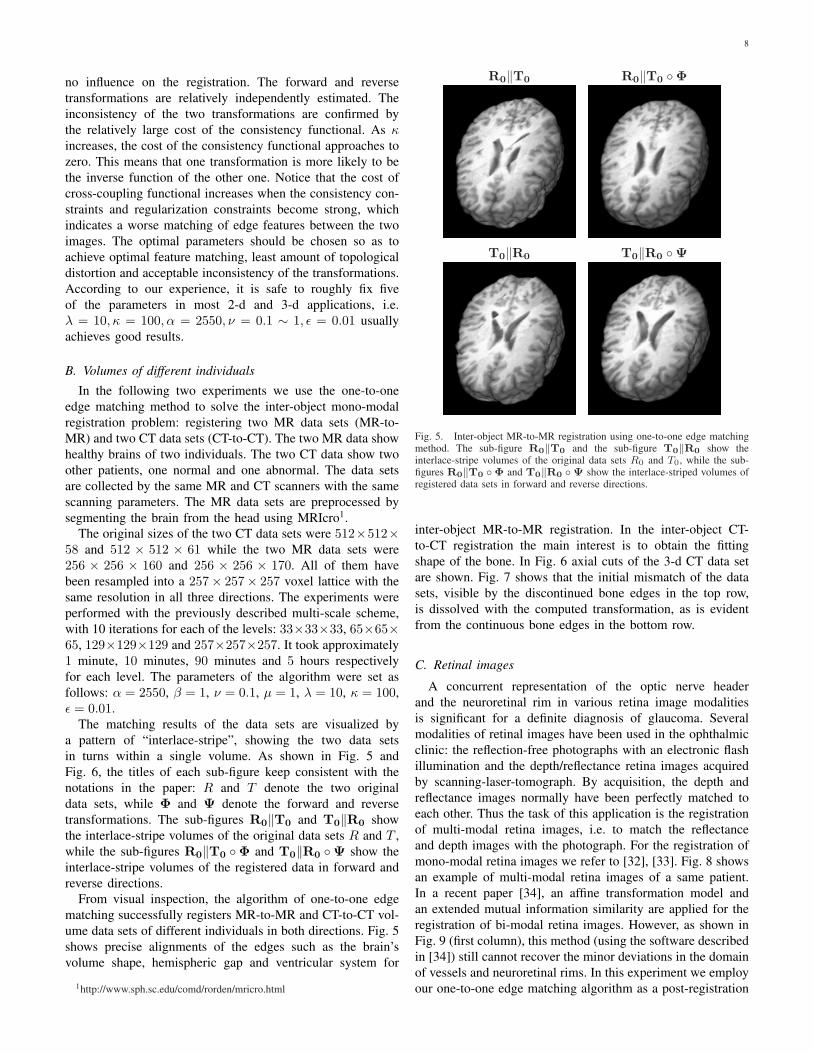
The matching results of the data sets are visualized bya pattern of “interlace-stripe”, showing the two data setsin turns within a single volume. As shown in Fig. 5 andFig. 6, the titles of each sub-figure keep consistent with thenotations in the paper: R and T denote the two originaldata sets, while Φ and Ψ denote the forward and reversetransformations. The sub-figures R0‖T0 and T0‖R0 showthe interlace-stripe volumes of the original data sets R and T ,while the sub-figures R0‖T0 Φ and T0‖R0 Ψ show theinterlace-stripe volumes of the registered data in forward andreverse directions.

From visual inspection, the algorithm of one-to-one edgematching successfully registers MR-to-MR and CT-to-CT vol-ume data sets of different individuals in both directions. Fig. 5shows precise alignments of the edges such as the brain’svolume shape, hemispheric gap and ventricular system for

1http://www.sph.sc.edu/comd/rorden/mricro.html

R0‖T0 R0‖T0 Φ

T0‖R0 T0‖R0 Ψ

Fig. 5. Inter-object MR-to-MR registration using one-to-one edge matchingmethod. The sub-figure R0‖T0 and the sub-figure T0‖R0 show theinterlace-stripe volumes of the original data sets R0 and T0, while the sub-figures R0‖T0 Φ and T0‖R0 Ψ show the interlace-striped volumes ofregistered data sets in forward and reverse directions.

inter-object MR-to-MR registration. In the inter-object CT-to-CT registration the main interest is to obtain the fittingshape of the bone. In Fig. 6 axial cuts of the 3-d CT data setare shown. Fig. 7 shows that the initial mismatch of the datasets, visible by the discontinued bone edges in the top row,is dissolved with the computed transformation, as is evidentfrom the continuous bone edges in the bottom row.

C. Retinal images

A concurrent representation of the optic nerve headerand the neuroretinal rim in various retina image modalitiesis significant for a definite diagnosis of glaucoma. Severalmodalities of retinal images have been used in the ophthalmicclinic: the reflection-free photographs with an electronic flashillumination and the depth/reflectance retina images acquiredby scanning-laser-tomograph. By acquisition, the depth andreflectance images normally have been perfectly matched toeach other. Thus the task of this application is the registrationof multi-modal retina images, i.e. to match the reflectanceand depth images with the photograph. For the registration ofmono-modal retina images we refer to [32], [33]. Fig. 8 showsan example of multi-modal retina images of a same patient.In a recent paper [34], an affine transformation model andan extended mutual information similarity are applied for theregistration of bi-modal retina images. However, as shown inFig. 9 (first column), this method (using the software describedin [34]) still cannot recover the minor deviations in the domainof vessels and neuroretinal rims. In this experiment we employour one-to-one edge matching algorithm as a post-registration

9

TABLE ISTUDY OF THE WEIGHT OF THE REGULARIZATION FUNCTIONAL EREG

Exp. λ CCC CREG CCON det DΦ det DΨFor Rev For Rev For Rev 1/ max min 1/ max min

B1 0.01 1982 2939 780.9 128.5 3.700 3.667 0.4736 −0.057 0.6933 0.4197B2 0.1 2221 2944 517.3 94.27 2.965 2.940 0.5671 0.088 0.7617 0.5195B3 1 2709 2971 181.2 59.70 2.032 2.029 0.7348 0.4737 0.7358 0.4899B4 5 3120 3050 44.24 27.27 1.149 1.146 0.8738 0.7296 0.8518 0.7464B5 10 3328 3165 20.02 11.00 0.9419 0.9415 0.9253 0.8209 0.9070 0.8706B6 20 3517 3243 6.180 3.031 0.7674 0.7699 0.9403 0.9000 0.9479 0.9301B7 50 3550 3314 1.053 0.5344 0.1792 0.1833 0.9832 0.9599 0.9802 0.9724

CCC: Cross-coupling functional, CREG: Regularization functional, CCON: Consistency functional. The otherweight parameters were set as follows: α = 2550, β = 1, ν = 0.1, µ = 0.5, κ = 100.

TABLE IISTUDY OF THE WEIGHT OF CONSISTENCY FUNCTIONAL ECON

Exp. κ CCC CREG CCON det DΦ det DΨFor Rev For Rev For Rev 1/ max min 1/ max min

C1 0 3044 3121 28.85 41.87 3.054 3.047 0.8824 0.7507 0.8475 0.7950C2 50 3072 3137 27.19 45.13 0.7922 0.7891 0.8782 0.7251 0.8548 0.8136C3 100 3088 3157 27.24 42.26 0.3255 0.3249 0.8751 0.7495 0.8569 0.8230C4 200 3236 3115 32.69 25.19 0.1720 0.1720 0.8996 0.8032 0.8624 0.8246C5 300 3279 3154 27.72 17.06 0.1430 0.1426 0.9061 0.8046 0.8971 0.8824C6 400 3291 3169 26.82 17.50 0.1118 0.1165 0.9079 0.8086 0.8977 0.8758C7 500 3334 3182 24.74 32.82 0.0803 0.0803 0.9115 0.8170 0.9917 0.8794

ECC: Cross-coupling functional, EREG: Regularization functional, ECON: Consistency functional. The otherweight parameters were set as follows: α = 2550, β = 1, ν = 0.1, µ = 0.5, λ = 10.

R0‖T0 R0‖T0 Φ

T0‖R0 T0‖R0 Ψ

Fig. 6. Inter-object CT-to-CT registration using one-to-one edge matchingmethod. The sub-figure R0‖T0 and the sub-figure T0‖R0 show theinterlace-stripe volumes of the original data sets R0 and T0, while the sub-figures R0‖T0 Φ and T0‖R0 Ψ show the interlace-striped volumes ofregistered data sets in forward and reverse directions.

Fig. 7. The matching of skulls in CT-to-CT registration. Above: Interlace-stripe volumes of skulls of original data sets. Bottom: Interlace-stripe volumesof matched skulls.

to compensate such small deviations of fine vessels.The images are pre-processed in the following way: ex-

tracting the green channel of the photograph as the inputfor the registration, affinely pre-registering the photograph toreflectance and depth images using the automatic softwaredescribed in [34], sampling the pre-registered images in amesh of 257 × 257. The algorithm is run for 10 iterations

10

Fig. 8. Multi-modal retina images of a same patient: photograph (left), depthimage (middle) and reflectance image (right).

Fig. 9. The example of post-registration of bi-modal retina images usingone-to-one edge matching. The photograph is registered with the depthimage (top) and the reflectance image (bottom). A published registrationmethod for bi-modal retina images cannot fully recover the minor deviationsof fine structures (first column). The forward and reverse transformationsestimated by the one-to-one edge matching successfully remove such minormismatching.

in three levels, which takes less than three minutes altogether.The parameters of the algorithm are set as follows: α = 2550,β = 1, ν = 0.1, µ = 0.5, λ = 10, κ = 100, ε = 0.01. FromFig. 9, one can observe that most minor deviations in thedomain of vessels are compensated by the computed non-rigidtransformations. Note that in this example with fine elongatedstructures, different from more volumetric image structuresin the other applications, an affine pre-registration is used tocompensate the large initial mismatch and to avoid gettingstuck in a local minimum.

D. Photographs of neurosurgery

In neocortical epilepsy surgery, the tumor (lesion) maybe located adjacent to, or partly within, so-called eloquent(functionally very relevant) cortical brain regions. For a safeneurosurgical planning, the physician needs to map the ap-pearance of the exposed brain to the underlying functionality.Usually, an electrode is placed on the surface of the brain inthe first operation for electrophysiological examination of theunderlying brain functionalities, then the photograph withinthe tested anatomical boundaries is colored according to thefunction of electrode contacts. On the other hand, the pre-operative 3-d MR data set contains the information of theunderlying tumor and healthy tissue as well. In the secondoperation, the registered photograph and MRI volume areused together to perform the cutting without touching eloquent

areas. At the moment a neocortical expert needs to manuallyrotate the 3-d MR to find the best 2-d projection matchingto the photographs. However, due to the different acquisitionsand the brain shift during surgery, the photograph and MRprojection cannot be accurately aligned. In this experiment, wemake use of our one-to-one edge matching algorithm to refinethe matching between a 2-d digital photograph of epilepsysurgery to the projection of 3-d MR data of the same patient.

The digital photographs of the exposed cortex are takenwith a handheld Agfa e1280 digital camera (Agfa, Cologne,Germany) from the common perspective of the neurosurgeon’sview. The high-resolution 3-d data set is acquired accordingto the T1-weighted MR imaging protocol (TR 20, TE 3.6,flip angle 30, 150 slices, slice thickness 1mm) using 1.5Tesla Gyroscan ACS-NT scanner (Philips Medical Systems).The brain is automatically extracted from the MRI volumeusing the SISCOM module of the Analyze software (MayoFoundation, Rochester, MN). For both the photograph and theMR projection, the regions of interest are manually selectedby a physician.

Fig. 10 shows the input images, preprocessed images,interlace-stripe registered and unregistered images. In sub-figure R0 the digital photograph shows the exposed lefthemisphere from an intraoperative viewpoint, the frontal lobeon the upper left, the parietal lobe on the upper right andparts of the temporal lobe on the bottom. The surface withthe gyri and sulci and the overlying vessels are clearly visible.Alongside, sub-figure T0 displays the left-sided view of therendered MR volume in the corresponding parts. Comparingsub-figures R0 and T0, one can notice that the undesiredsurface vessels and reflectance flash are strongly presented inthe digital photograph, while the MR projection images clearlydisplay the desired edge features. The photographic imageand the projection image were preprocessed by appropriateGIMP filter chains for edge enhancement. The preprocessedimages are displayed in sub-figures “R0 preprocessed” and“T0 preprocessed”, respectively. Both images were resampledto 2049× 2049 pixels. The algorithm was run from level 3 tolevel 11. We note that the values of the parameters β andµ are quite different from the other examples. The reasonis that the image modalities of the photograph and the MRprojection differ largely from each other. The two parametersare set as β = 100 and µ = 0.1, so that both phase fieldfunctions W and V clearly represent the edge features on thebrain and have comparable influence on the registration. Insub-figures T0‖R0 and R0‖T0, the interlace-stripe imagesillustrate the mismatch of photograph and MR projection. Sub-figures T0‖R0 Ψ and R0‖T0 Φ show that the methodgreatly refines the matching of the desired edge features.Especially the brain sulci and gyri, which are significant forneurosurgery, are nearly perfectly aligned to each other. Wehave implemented a mutual information algorithm in the sameFinite Element framework (including the step sized controlled,regularized, multi-scale descent) for a comparison. Overall,our method gives comparable results in most cases, especiallywhen dealing with coarse structures. However, in this examplethat contains a large number of fine structures, the edge-basedmatching gives better alignment. The zoom views of local

11

R0 T0 R0 prepr. T0 prepr.

R0‖T0 R0‖T0 Φ

T0‖R0 T0‖R0 Ψ

Fig. 10. Experimental results of matching a neurosurgery photograph of asection of the brain with its MR projection. All the sub-figures only display theregion of interest: the exposed cortex. R0: The photograph of the exposedleft hemisphere from an intraoperative view point. T0: The projection ofthe MR volume, whose orientation is specified by physicians. PreprocessedR0 and Preprocessed T0: The preprocessed photograph and MR projection.R0‖T0 and T0‖R0: The interlace-strip images of unregistered photographand MR projection. R0‖T0 Φ and T0‖R0 Ψ: The interlace-strip imagesof registered photograph and MR projection.

regions in Fig. 11 show that the edge-matching method canachieve a better alignment of fine structures than the mutualinformation based registration.

E. Motion estimation for frame interpolation

Temporal interpolation of video frames in order to increasethe frame rate requires the estimation of a motion field(transformation). Then pixels in the intermediate frame areinterpolated along the path of the motion vector. In this section,we give a proof of concept that the one-to-one edge matchingmethod can be used for this application. For a review oftechniques of frame interpolation, we refer to [35], [36].

We perform our test on the Susie sequence and interpolateframe 58 in Fig. 12. We use a 257 × 257 cropped versionfor the experiment. Frames 57, 58 and 59 are denoted asF57, F58 and F59 respectively. The forward transformationΦ : F57 → F59 and reverse transformation Ψ : F59 → F57 areestimated by the one-to-one edge matching with the parametersetting: α = 2550, β = 1, ν = 0.1, µ = 1, λ = 10, κ = 100,ε = 0.01. Frame 58 is interpolated as: F58 = 0.5 × (F57 0.5Φ + F59 0.5Ψ). It is compared with a standard blockmatching algorithm using an adaptive rood pattern search [37],16 × 16 blocks and a search range of [−16, 16] in thehorizontal and vertical directions. The experimental resultsshow that the block matching algorithm produces blocky andnoisy motion fields, while the one-to-one edge matching based

edge matching mutual information

Fig. 11. Comparison of one-to-one edge matching (left) and the mutualinformation based matching (right). The two algorithms are implemented in asame Finite Element framework including the step size controlled, regularizedmulti-scale descent. The first row shows how the pre-processed images areregistered by the two methods. The last two rows show zoomed views of localregions in the registered images. The comparison shows that one-to-one edgematching comes along with a significantly better registration of fine structures.

motion estimation gives an excellent visual quality of frameinterpolation.

V. CONCLUSION AND SUMMARY

This paper presents a new algorithm for the edge matchingproblem. It simultaneously performs the following three tasks:detecting the edge features from two images, computingtwo dense warping functions in both forward and reversedirections to match the detected features, and constrainingeach dense warping function to be the inverse of the other.An adaptive regularized gradient descent, in the frameworkof multi-resolution Finite Element approximation, enables thealgorithm to efficiently find the pair of dense transformations.The algorithm has been tested on T1-/T2-MR volume data.It is found that the proposed algorithm successfully preservedthe topology of the images and the bijectivity of the mappings.The paper also shows that the algorithm has been successfullyused in four applications: registration of inter-object volumedata, registration of retinal images, matching photographs ofneurosurgery with its volume data and motion estimation forframe interpolation.

ACKNOWLEDGMENT

The authors acknowledge Rudiger Bock (Chair of PatternRecognition, Erlangen-Nurnberg University) for providing the

12

Fig. 12. Motion estimation for frame interpolation. Top: Original frame 57,58 and 59 of Susie sequence. Bottom: the interpolated frame 58 using simplyaveraging (left), one-to-one edge matching motion estimation (middle) andstandard block matching motion estimation (right).

retinal images and the retina registration software for com-parison. The authors thank Michael Fried (Chair of AppliedMathematics, Erlangen-Nurnberg University) for his valuablecomments and suggestions. The authors thank HipGraphicsInc. for providing the software (InSpace) for volume rendering.

REFERENCES

[1] D. Mumford and J. Shah, “Optimal approximation by piecewise smoothfunctions and associated variational problems,” Communications on Pureand Applied Mathematics, vol. 42, pp. 577–685, 1989.

[2] J. M. Morel and S. Solimini, Variational methods in image segmentation.Cambridge, MA, USA: Birkhauser Boston Inc., 1995.

[3] T. F. Chan, B. Y. Sandberg, and L. A. Vese, “Active contours withoutedges for vector–valued images,” Journal of Visual Communication andImage Representation, vol. 11, pp. 130–141, 2000.

[4] T. F. Chan and L. A. Vese, “Active contours without edges,” IEEETransactions on Image Processing, vol. 10, no. 2, pp. 266–277, 2001.

[5] M. Fried, “Multichannel image segmentation using adaptive finite ele-ments,” Computing and Visualization in Science, to appear.

[6] M. Droske and W. Ring, “A Mumford-Shah level-set approach forgeometric image registration,” SIAM Appl. Math., 2007, to appear.

[7] M. Droske, W. Ring, and M. Rumpf, “Mumford-shah based registration,”Computing and Visualization in Science manuscript, 2007, to appear.

[8] T. Kapur, L. Yezzi, and L. Zollei, “A variational framework for jointsegmentation and registration,” Proceedings of the IEEE Workshop onMathematical Methods in Biomedical Image Analysis (IEEE CVPR -MMBIA), pp. 44–51, 2001.

[9] T. F. Chan and L. A. Vese, “Active contours without edges,” IEEETransactions on Image Processing, vol. 10, no. 2, pp. 266 – 277, 2001.

[10] P. Rogelj and S. Kovacic, “Symmetric image registration,” MedicalImage Analysis, vol. 10, pp. 484–493, 2006.

[11] G. E. Christensen and H. J. Johnson, “Consistent image registration,”IEEE Transactions on Medical Imaging, vol. 20, no. 7, pp. 568–582,2001.

[12] H. J. Johnson and G. E. Christensen, “Consistent landmark and intensity-based image registration,” IEEE Transactions on Medical Imaging,vol. 21, no. 5, pp. 450–461, 2002.

[13] D. Rueckert, A. Frangi, and J. Schnabel, “Automatic construction of 3-dstatistical deformation models of the brain using nonrigid registration,”IEEE Transactions on Medical Imaging, vol. 22, no. 8, pp. 1014–1025,2003.

[14] S. Marsland, C. Twining, and C. Taylor, “Groupwise non-rigid registra-tion using polyharmonic clamped-plate splines,” in Sixth InternationalConference on Medical Image Computing and Computer-Assisted In-tervention (MICCIA’03), ser. LNCS, R. E. Ellis and T. M. Peters, Eds.Montreal: Springer Verlag, 2003, pp. 246–250.

[15] C. Sorzano, P. Thevenaz, and M. Unser, “Elastic registration of biolog-ical images using vector-spline regularization,” IEEE Transactions onBiomedical Engineering, April 2005.

[16] I. Arganda-Carreras, C. Sorzano, R. Marabini, J. Carazo, C. Ortiz-De-Solorzano, and J. Kybic, “Consistent and elastic registration ofhistological sections using vector-spline regularization,” in workshop ofthe 9th European Conference on Computer Vision (CVAMIA-06), R. E.Ellis and T. M. Peters, Eds. In Press, 2006.

[17] J. Han, B. Berkels, M. Rumpf, J. Hornegger, M. Droske, M. Fried,J. Scorzin, and C. Schaller, “ A Variational Framework for JointImage Registration, Denoising and Edge Detection,” in ProceedingsBildverarbeitung fur die Medizin , H. Handels, J. Ehrhardt, A. Horsch,H. Meinzer, and T. Tolxdorff, Eds. Berlin: Springer, 2006, pp. 246–250.

[18] L. Ambrosio and V. M. Tortorelli, “Approximation of functionals de-pending on jumps by elliptic functionals via Γ-convergence,” Commu-nications on Pure and Applied Mathematics, vol. 43, pp. 999–1036,1990.

[19] R. March, “Visual reconstructions with discontinuities using variationalmethods,” Image and Vision Computing, vol. 10, no. 1, pp. 30–38, 1992.

[20] J. Modersitzki, Numerical Methods for Image Registration. Oxford:Oxford University Press, 2004.

[21] J. Ashburner, J. Andersson, and K. Friston, “High-dimensional nonlinearimage registration using symmetric priors,” NeuroImage, vol. 9, pp. 619–628, 1999.

[22] C. Broit, “Optimal registration of deformed images,” Ph.D. dissertation,University of Pensylvania, 1981.

[23] G. E. Christensen, S. C. Joshi, and M. I. Miller, “Volumetric transforma-tion of brain anatomy,” IEEE Transactions on Medical Imaging, vol. 16,no. 6, pp. 864–877, 1997.

[24] M. Bro-Nielsen and C. Gramkow, “Fast fluid registration of medicalimages.” Lecture Notes in Computer Science, vol. 1131, pp. 267–276,1996.

[25] M. E. Gurtin, An Introduction to Continuum Mechanics. Orlando,Florida: Academic Press, 1981.

[26] M. Droske and M. Rumpf, “A variational approach to non-rigid mor-phological registration,” SIAM Appl. Math., vol. 64, no. 2, pp. 668–687,2004.

[27] R. Schaback and H. Werner, Numerische Mathematik, 4th ed. Berlin:Springer-Verlag, 1992.

[28] O. Scherzer and J. Weickert, “Relations between regularization anddiffusion filtering,” Journal of Mathematical Imaging and Vision, vol. 12,no. 1, pp. 43–63, 2000.

[29] U. Clarenz, S. Henn, and K. Rumpf, M. Witsch, “Relations betweenoptimization and gradient flow methods with applications to imageregistration,” in Proceedings of the 18th GAMM Seminar Leipzig onMultigrid and Related Methods for Optimisation Problems, 2002, pp.11–30.

[30] U. Clarenz, M. Droske, and M. Rumpf, “Towards fast non–rigid registra-tion,” in Inverse Problems, Image Analysis and Medical Imaging, AMSSpecial Session Interaction of Inverse Problems and Image Analysis,vol. 313. AMS, 2002, pp. 67–84.

[31] P. Kosmol, Optimierung und Approximation. de Gruyter Lehrbuch,1991.

[32] A. Can, C. V. Stewart, B. Roysam, and H. L. Tanenbaum, “A feature-based, robust, hierarchical algorithm for registering pairs of images ofthe curved human retina,” IEEE Transactions on pattern analysis andmachine intelligence, vol. 24, no. 3, 2002.

[33] ——, “A feature-based technique for joint, linear estimation of high-order image-to-mosaic transformations: mosaicing the curved humanretina,” IEEE Transactions on pattern analysis and machine intelligence,vol. 24, no. 3, 2002.

[34] L. Kubecka and J. Jan, “Registration of bimodal retinal images - im-proving modifications,” in Proceedings of the 26th Annual InternationalConference of the IEEE Engineering in Medicine and Biology Society(EMBC 2004), vol. 3, 2004, pp. 1695– 1698.

[35] R. Krishnamurthy, J. Woods, and P. Moulin, “Frame interpolation andbidirectional prediction of video usingcompactly encoded optical-flowfields and label fields,” IEEE Transactions on Circuits and Systems forVideo Technology, vol. 9, pp. 713–726, 1999.

[36] H. A. Karim, M. Bister, and M. U. Siddiqi, “Multiresolution motionestimation for low-rate video frame interpolation,” Journal on AppliedSignal Processing, vol. 11, pp. 1708–1720, 2004.

[37] Y. Nie and K.-K. Ma, “Adaptive rood pattern search for fast block-matching motion estimation,” IEEE Transactions on Image Processing,vol. 11, pp. 1442 – 1449, 2002.