University of Alberta

Multivariate Analysis of Diverse Data for Improved Geostatistical Reservoir

Modeling

by

Sahyun Hong

A thesis submitted to the Faculty of Graduate Studies and Research

in partial fulfillment of the requirements for the degree of

Doctor of Philosophy

in

Mining Engineering

Department of Civil and Environmental Engineering

©Sahyun Hong

Fall 2010

Edmonton, Alberta

Permission is hereby granted to the University of Alberta Libraries to reproduce single copies of this thesis and to lend

or sell such copies for private, scholarly or scientific research purposes only. Where the thesis is converted to, or otherwise made available in digital form, the University of Alberta will advise potential users of the thesis of these

terms.

The author reserves all other publication and other rights in association with the copyright in the thesis and, except as herein before provided, neither the thesis nor any substantial portion thereof may be printed or otherwise reproduced in

any material form whatsoever without the author's prior written permission.

Examining Committee

Dr. Clayton Deutsch (Supervisor) , Civil and Environmental Engineering

Dr. Jozef Szymanski (Chair and Examiner), Civil and Environmental Engineering

Dr. Jerry Jensen (External Examiner), Chemical and Petroleum Engineering, Univ. of Calgary

Dr. Peter Hooper (Examiner), Mathematical and Statistical sciences

Dr. Hooman Askari-Nasab (Examiner), Civil and Environmental Engineering

Abstract Improved numerical reservoir models are constructed when all available diverse data sources are

accounted for to the maximum extent possible. Integrating various diverse data is not a simple

problem because data show different precision and relevance to the primary variables being

modeled, nonlinear relations and different qualities. Previous approaches rely on a strong

Gaussian assumption or the combination of the source-specific probabilities that are individually

calibrated from each data source.

This dissertation develops different approaches to integrate diverse earth science data. First

approach is based on combining probability. Each of diverse data is calibrated to generate

individual conditional probabilities, and they are combined by a combination model. Some

existing models are reviewed and a combination model is proposed with a new weighting scheme.

Weakness of the probability combination schemes (PCS) is addressed. Alternative to the PCS,

this dissertation develops a multivariate analysis technique. The method models the multivariate

distributions without a parametric distribution assumption and without ad-hoc probability

combination procedures. The method accounts for nonlinear features and different types of the

data. Once the multivariate distribution is modeled, the marginal distribution constraints are

evaluated. A sequential iteration algorithm is proposed for the evaluation. The algorithm

compares the extracted marginal distributions from the modeled multivariate distribution with the

known marginal distributions and corrects the multivariate distribution. Ultimately, the corrected

distribution satisfies all axioms of probability distribution functions as well as the complex

features among the given data.

The methodology is applied to several applications including: (1) integration of continuous

data for a categorical attribute modeling, (2) integration of continuous and a discrete geologic

map for categorical attribute modeling, (3) integration of continuous data for a continuous

attribute modeling. Results are evaluated based on the defined criteria such as the fairness of the

estimated probability or probability distribution and reasonable reproduction of input statistics.

Acknowledgement First of all, I would like to thank Dr. Clayton V. Deutsch for his guidance, patience and

unexhausted ideas. Both his mentorship and friendship made my times during my PhD exciting

and enjoyable.

My special thanks go to the industrial sponsors of Centre for Computational Geostatistics

(CCG) company members for their financial supports. Also, the financial supports for this

research provided by Provost Doctoral Entrance Award and J Gordon Kaplan Graduate Student

Award in the University of Alberta are greatly appreciated.

I would like to thank my parents for their endless love, support and for always having

confidence in me. My children Lindsay and Lynnwoo give me a lot of joy and happiness in my

life. Most importantly, I want to thank my wife, Jina. I would not be here without your love and

support.

Contents

Chapter 1 Introduction................................................................................................... 1 1.1  Primary and Secondary Data ................................................................................................ 3 1.2  Data Integration .................................................................................................................... 4 1.3  Problem Setting .................................................................................................................... 7 1.4  Dissertation Outline ............................................................................................................ 10 

Chapter 2 Probabilistic Reservoir Modeling .............................................................. 12 2.1  Probabilistic Approach ....................................................................................................... 12 2.2  Geostatistical Techniques for Reservoir Modeling ............................................................ 13 

2.2.1  Random Function Concept ....................................................................................... 13 2.2.2  Measure of Spatial Dependence ............................................................................... 14 2.2.3  Representative Statistics ........................................................................................... 16 2.2.4  Geostatistical Estimation Algorithms ....................................................................... 18 2.2.5  Geostatistical Simulation .......................................................................................... 23 

2.3  Discussions ......................................................................................................................... 23 

Chapter 3 Probability Combination Schemes ............................................................ 25 3.1  Combining Probabilities ..................................................................................................... 26 3.2  Simple Combination Models .............................................................................................. 27 

3.2.1  Conditional Independence Model ............................................................................. 27 3.2.2  Permanence of Ratios Model (PR model) ................................................................ 28 

3.3  Weighted Combination Model ........................................................................................... 32 3.3.1  Tau model ................................................................................................................. 32 3.3.2  Lamda Model ............................................................................................................ 36 

3.4  1-D Example ....................................................................................................................... 41 3.5  Applications of Combining Approaches ............................................................................ 46 3.6  Accuracy Assessment ......................................................................................................... 54 3.7  Building High Resolution Stochastic Model ...................................................................... 57 3.8  Remarks on the PCS ........................................................................................................... 60 

Chapter 4 Direct Modeling of Multivariate Distribution .......................................... 62 4.1  Modeling the Multivariate Probability Densities ............................................................... 63 4.2  Marginal Conditions of the Multivariate Distribution ........................................................ 68 

4.2.1  Imposing Marginal Conditions ................................................................................. 70 4.2.2  Examples .................................................................................................................. 72 

4.3  Convergence of Sequential Marginal Fitting Algorithm .................................................... 76 

Chapter 5 Applications of Multivariate Distribution Modeling ............................... 81 5.1  Integrating Multiple Soft Secondary Data .......................................................................... 82 

5.1.1  Amoco Examples ...................................................................................................... 83 5.1.2  West African Reservoir Example ............................................................................. 91 

5.1.3  Accounting for Large Scale Secondary Data .......................................................... 107 5.2  Debiasing with Multiple Soft Secondary Data ................................................................. 114 5.3  Integration of Soft Secondary and Geologic Map ............................................................ 118 5.4  Discussions ....................................................................................................................... 130 

Chapter 6 Advanced Application of the Multivariate Distribution Modeling ...... 131 6.1  Bayesian Updating ............................................................................................................ 131 

6.1.1  Resolution of Bayesian Updating ........................................................................... 132 6.1.2  Accounting for Non-linear Relations between Primary and Secondary Variables . 136 6.1.3  Examples ................................................................................................................ 141 

6.2  Discussions ....................................................................................................................... 150 

Chapter 7 Summary and Conclusions ...................................................................... 151  Bibliography .................................................................................................................. 155  A Symbols and Selected Terms .................................................................................... 161  Appendix A Factorial Kriging for Reservoir Feature Identification and Extraction......................................................................................................................................... 163

List of Tables Table 3.1: An example of the fairness measure for categorical variable ····························· 56

Table 3.2: Comparison of the reproduced global proportions from the generated realizations with

the input proportion p(s=1)=0.514 and p(s=2)=0.486. ·················································· 59

Table 5.1: Linear correlation among variables ··························································· 93

 

List of Figures Figure 1.1: Various scales and reservoir coverage of data (modified from Harris and Langan, 1997) ············································································································ 3

Figure 1.2: A workflow of geostatistical reservoir modeling in the presence of multiple secondary data. ············································································································· 6

Figure 1.3: An illustration for showing two different methods to estimate final conditional probability given multiple secondary data. ································································ 8

Figure 1.4: An example illustrating incremental information impact on the probability estimate. Probabilities are estimated with and without accounting for data redundancy. ······················· 9

Figure 3.1: A graphical illustration for calculating weights using weight calibration method 1. Weights are calculated based on the differences between true and combined probabilities. ······ 39

Figure 3.2: 1-D example along the horizontal transect. Modeling for the binary category is considered. Three conditioning secondary data D1,D2 and D3 are assumed to redundant since the probabilities p(s|Di) are positively correlated. The global proportion p(s) and the primary hard data ( ) are shown. ··························································································· 41

Figure 3.3: The combined probability using the conditional independence model (pCI). ·········· 42

Figure 3.4: The combined probability using the Lamda model with the first calibration method. To avoid the numerical instability, an artificial small value (ε) is injected to the calibration equation and the results become different based on the used small values. ·························· 43

Figure 3.5: The combined probability using the Lamda model with the second calibration method. ·················································································································· 45

Figure 3.6: The resulting combined probability from the different models: conditional independence and the Lamda model with different calibration approaches. ························· 46

Figure 3.7: 62 well location map of Amoco data. Scales are in ft. ··································· 46

Figure 3.8: A seismic amplitude map (left), probability distributions calibrated from the 62 wells (centre), and the derived facies probability map (right). ················································ 47

Figure 3.9: The trend of facies 1 generated by simple indicator kriging with isotropic variogram. ·················································································································· 48

Figure 3.10: A deterministic facies model is generated by subject drawing the facies boundary. Facies proportions are derived from the deterministic model by applying a moving window. ···· 48

Figure 3.11: The estimated facies probabilities from three different combination schemes: the conditional independence (top), Lamda model with calibration method 1 (middle) and 2 (bottom). ·················································································································· 51

Figure 3.12: Cross plots for showing the non-convex behavior of the combined probability; the input individual probabilities p(s=1|Di) for i=1,2,3 and the combined probabilities p(s=1|D1,D2,D3) from the different combination methods are plotted. Plotting is made when the p(s|Di) for i=1,2,3 are all greater than the global proportion p(s=1)=0.514. ················································ 53

Figure 3.13: Small example showing the risk of the classical accuracy measure. ·················· 55

Figure 3.14: Fairness plots of the combined probabilities from different combination models. The plotted fairness measure is averaged over facies s=1,2. ················································ 57

Figure 3.15: Variogram of indicator variable representing facies: experimental variograms (dots) and their fitted variograms (lines). ········································································· 58

Figure 3.16: Reproduced variograms (dashed lines) from the 21 realizations that are made by different simulation scenarios: simulation with well data only (SISIM) and with integrating secondary derived probabilities obtained from the different methods (SISIM with pCI, pLamda1, pLamda2). The input variogram is shown as heavy sold line. ············································ 60

Figure 4.1: Examples of 1-D kernel density estimates with varying bandwidths h. Standard deviation of experimental data σdata is 3.5 and h is arbitrarily chosen with approximately 14%, 28% and 57% of σdata, respectively. ·············································································· 64

Figure 4.2: Schematic illustration for comparing the reproduced with the known marginal distribution. Since the joint distribution is modeled with the limited well samples its reproduced marginal is not consistent with the (very well-known) marginal pdf which is a distribution of secondary data. ······························································································· 70

Figure 4.3: The example of the marginal fitting algorithm for the continuous variable. Initial bivariate pdf is shown in the left. The actual marginal and reproduced marginal distributions are shown as sold and dashed lines, respectively. The fitting algorithm updates the initial pdf as shown in the right. Each marginal pdf is exactly reproduced. ········································· 74

Figure 4.4: The effect of the initial distributions when applying the algorithm. Three different cases generate different final bivariate distributions with the same accuracy of marginal errors. 76

Figure 4.5: Small discrete example showing the convergence. ········································ 77

Figure 5.1: Cross plot of collocated secondary data. ···················································· 83

Figure 5.2: The modeled bivariate distribution of secondary data f(y1,y2). The experimental 4225 data points are overlaid. ····················································································· 84

Figure 5.3: The estimated joint probability distributions. The 3-D distribution is displayed separately for each facies category. ········································································ 85

Figure 5.4: The joint probability distributions modeled by kernel estimator (left column) and modified distributions constrained by the imposed marginal conditions (right column). The arrow shown in the middle represents the direction of marginal fitting: two horizontal directions are to compare the probability of facies p(s), and vertical direction is to compare the secondary data distribution f(y1,y2). ·························································································· 87

Figure 5.5: Averaged marginal errors versus iterations for Amoco test data. ························ 88

Figure 5.6: Estimated facies probability using the updated joint distribution and histograms of estimated soft values. ························································································ 89

Figure 5.7: Fairness plots of the local probabilities for the Amoco case. Actual fractions with few samples are shown as open circles and they are not used to evaluate the estimated local probability. ···································································································· 90

Figure 5.8: The reproduced variograms in NS direction from 21 realizations: SISIM without secondary data (left) and with secondary derived probability that are obtained from the multivariate pdf modeling technique. ····································································· 90

Figure 5.9: Interpreted stratigraphic units over the reservoir. Three massive bodies are interpreted with individual meandering channels. Four main facies are identified: high net-to-gross channel, sand, and low net-to-gross shale and shaly sand. ························································ 91

Figure 5.10: 3-D view of the first seismic attribute. ····················································· 92

Figure 5.11: Distributions of seismic attributes sampled from well locations. ······················ 93

Figure 5.12: Scatter plots of exhaustive seismic values and its modeled probability distributions. ·················································································································· 94

Figure 5.13: Scatter plots of the selected seismic variables (denoted as Y1 and Y2) with different facies types. The means of Y1 and Y2 for each facies are plotted in the bottom. ··················· 96

Figure 5.14: The modeled initial joint distributions (before constraining). Product kernel estimator is considered for multivariate nonparametric modeling. One reproduced marginal distribution is shown in the bottom. ······································································· 97

Figure 5.15: The corrected joint distribution f(s,y1,y2) after applying marginal constraints. ······· 98

Figure 5.16: The joint distributions modeled with different conditions of kernel bandwidths. Based on theoretical kernel bandwidth hopt, 60% changes are applied. ······························· 99

Figure 5.17: Cross plot of the actual secondary values and their corresponding bin values. 50 bins are defined for numerical joint density modeling and this level of binning does not invoke discretization errors. ······················································································· 100

Figure 5.18: Histograms of the secondary derived facies probability. Averages of each histogram are close to the declustered global proportions. ························································ 101

Figure 5.19: The improvements in the correlation between the used seismic and facies. ········ 101

Figure 5.20: Fairness plots for the West African reservoir example. Actual fractions defined in section 3.6 are plotted against predicted probabilities. The actual fractions are reasonably all on the diagonal line for facies 1, 4 and overall. ···························································· 102

Figure 5.21: Experimental and modeled variograms for four facies. ······························· 104

Figure 5.22: E-type estimate of channel facies from 21 realizations without secondary data. ·· 105

Figure 5.23: E-type estimate of channel facies from 21 realizations with secondary data. ······ 105

Figure 5.24: Variogram reproductions from the 21 realizations. Distances in horizontal and vertical directions are in meter and ft, respectively. ··················································· 106

Figure 5.25: A synthetic reference images and well data extracted from the reference image. Coordinates are all in meter. ·············································································· 108

Figure 5.26: Two simulated secondary data. Vertical resolution is 5 times larger than the modeling cell size. Kernel method is used for the modeling of bivariate relation. ··············· 109

Figure 5.27: Cross plots of block secondary values and facies proportions from 6 vertical wells. ················································································································ 109

Figure 5.28: For visualizing purposes, the facies proportions from the true image and estimated proportions are shown in the left column. Right column shows the scatter plots between the true and estimated proportions. ················································································ 111

Figure 5.29: Histograms of secondary derived facies proportions. Averages of each facies proportions are very close to the global representative facies proportions. ························ 113

Figure 5.30: Prepared reference image, well sample locations extracted from reference image and a simulated secondary data. Sample means are biased by 26% or above based on the true statistics. ····································································································· 115

Figure 5.31: Experimental data distribution and the modeled distribution f(s,y) based on sample data. The smooth line is a kernel estimator of bar chart. ············································· 116

Figure 5.32: The modified bivariate distributions by imposed marginal condition. A marginal distribution of secondary data is shown in the bottom. ··············································· 117

Figure 5.33: Reference image showing channel reservoir and 61 well data extracted from the reference image. X-Y coordinate is in meter. ·························································· 120

Figure 5.34: Two soft secondary variables are generated using the sequential Gaussian simulation and are correlated in a non-linear manner as shown in the cross plot of two variables. This non-linear pattern is to be accounted for by nonparametric technique. ·································· 121

Figure 5.35: A geologic map used for integrating with soft secondary data. ······················ 122

Figure 5.36: The modeled joint distribution of secondary data f(y1,y2,g), g=0,1. ·················· 123

Figure 5.37: The modeled initial joint distributions using the kernel estimator. ·················· 124

Figure 5.38: The corrected joint distributions under marginal constraints. ························ 125

Figure 5.39: Averaged marginal errors in % against the marginal fitting iterations. Errors are calculated by comparing the reproduced marginals from the joint distributions and the reference marginals. Marginal errors converge into very small percentage with 20 iterations where the corrected distributions become stable. ·································································· 126

Figure 5.40: Cross plot of actual and the binned soft secondary values. ··························· 127

Figure 5.41: The estimated probability of channel is shown at the middle. A 1-D section through X-X’ is plotted in the bottom showing the true values either 0 (non-channel) or 1 (channel) and the secondary guided channel probability (grey line). ················································ 128

Figure 5.42: The estimated probability of channel from integrating soft secondary and geology data, and soft secondary data only. Maps show the probability higher than 0.65: there is no special meaning of cutoff 0.65. This figure points out geologic heterogeneity is better reproduced and isolated pixels are reduced when considering both soft secondary and prior geologic information. ································································································· 129

Figure 6.1: An illustration of non-linear relation after individual normal score transform of each variable. ······································································································ 137

Figure 6.2: Workflow for the proposed approach······················································ 140

Figure 6.3: Simulated porosity used as secondary variable (left) for predicting permeability and sampled permeability at 62 well locations (right). ····················································· 141

Figure 6.4: Cross plot of normal scored permeability (primary) and porosity (secondary) variables. To check the bivariate normality, the generalized square distances are calculated from data and plotted against the analytical chi-square distances. Systematic differences represent non-biGaussian relation. ························································································ 142

Figure 6.5: Modeled bivariate pdf. Horizontal and vertical axes represent the primary and secondary variables. The described marginal fitting algorithm was applied to obtain this joint pdf. ················································································································ 142

Figure 6.6: Conditional means and variances obtained from the joint pdf modeled in a nonparametric way. Black dots (left) are the calculated conditional means of NS:per with respect to the varying secondary values NS:por. Open circles (right) are the conditional variances with respect to the secondary values. ·········································································· 144

Figure 6.7: Secondary data derived estimates and variances ········································· 144

Figure 6.8: Comparison of estimates and estimation variance from two different approaches. Solid and dashed lines represent estimate and estimation variance using linear assumption among variables and nonparametric approach, respectively. ················································· 145

Figure 6.9: Accuracy plots for the estimates from the linear assumption and the nonparametric method. ······································································································ 146

Figure 6.10: A trivariate pdf modeled by kernel density estimator with marginal correction process: the primary and two secondary variables are denoted as Z, Y1 and Y2, respectively. The lower order bivariate pdf reproduced from the trivariate pdf are checked with the input data scatter plots and distribution. ············································································· 147

Figure 6.11: The estimates and estimation variances from two different methods. Upper low shows the estimates from the linear and nonparametric approach given the secondary data values Y1 and Y2. Bottom low shows the estimation variance. Nonlinearity in the estimates and estimation variances is obvious. ·········································································· 148

Figure 6.12: The estimates and estimation variances from integrating two secondary data using the nonparametric method for all locations u∈A. ······················································ 149

Figure 6.13: Accuracy plots for the results from the linear assumption (left) and nonparametric (right). Goodness statistics are shown on each plot. ·················································· 149 

1

Chapter 1

Introduction

Building numerical reservoir models is an intermediate but essential step for reservoir

management. Numerical models are used to plan new wells, calculate overall hydrocarbon

reserves, predict the reservoir performance in a flow simulator, and to analyze the uncertainty in

reservoir performance forecasts. Accurate reservoir models may lead to accurate predictions of

reservoir performance and improve reservoir management decisions with less uncertainty. Thus,

constructing numerical geologic models is an important step in reservoir management. Accurate

reservoir modeling, however, is difficult to achieve given the few directly measured data; the

reservoir properties such as facies, porosities, permeabilities, hydrocarbon saturations, occurrence

of fault are typically sampled at very few well locations. These reservoir properties are

heterogeneous and the distribution is never known exactly. Moreover, these properties are highly

coupled with complex geological structures. Due to these reasons it is not desirable to consider

only one quantitative description of a reservoir in a deterministic way (Haldorsen and Damsleth,

1990; Ballin et al., 1992). Equally probable descriptions or realizations of the reservoir are useful

to account for a lack of knowledge or uncertainty. Stochastically generated realizations allow

quantifying the uncertainty in the spatial distribution of reservoir properties and the distribution

of reservoir responses. Risk-qualified decision making techniques can be applied with multiple

realizations to reach a final decision (Srivastava, 1987).

Improved numerical reservoir models can be constructed when all available diverse data are

integrated to the maximum extent possible. The uncertainty in the model will generally decrease

with additional data sources. The reservoir attribute of modeling is supplemented by additional

information from various data sources. Diverse data are commonly available in petroleum

applications. These data include seismic related attributes from the seismic exploration,

2

conceptual geologic map from geologist or analogue data and historical production data from

well test. Other reservoir related information such as reservoir top surface, bottom surface and

thickness are useful data though they do not arise from different sources.

The main purpose of reconciling these diverse data is to provide accurate models and reduce

the uncertainty in the reservoir performance predictions in a consistent manner. However, there

are some issues that should be addressed when accounting for the secondary data. Each data

source carries information on the reservoir properties at different scales and with varying levels of

precision (Deutsch and Hewett, 1996). For example, 3D seismic attributes data contain

information on reservoir properties such as the spatial distribution of major faults, lithofacies,

porosity and fluids carried by their respective porous rock and they are imprecisely related to the

reservoir properties of consideration (Lumley et al., 1997). Geologic map data reflect a geologic

realism of reservoir created by complex physical process. A certain geologic feature such as

connectivity of high and low permeable rock that is a first-order impact on fluid flow can be

better understood from incorporating geologic map. Production data consists of time series of

pressure and flow rate that are direct measurements of reservoir performance. Incorporating

production data could provide a coarse scale map of permeability. Despite increasing availability

of secondary data, integrating those data is not straightforward because of the various scale of

each data. For instance, seismic data are typically at a coarser vertical resolution than geological

models, usually 10 – 100 times the resolution of a geologic modeling cell although the horizontal

resolution of seismic data is often comparable with the modeling cells. A geologic map may be

established from a geologist’s hand-drawing or analog database from similar depositional settings

at a relatively large scale. Production data are measured in a single point but represent a large

volume and they are interpreted as effective properties representing that volume. All these issues

related with scale, precision and coverage should be overcome when constructing numerical

models. Figure 1.1 illustrates the varying degree of vertical resolution and reservoir coverage of

available data.

3

Figure 1.1: Various scales and reservoir coverage of data (modified from Harris and Langan, 1997)

1.1 Primary and Secondary Data

In geostatistical terminology, the data used for modeling can be divided into two types: primary

and secondary data. Direct measurements of target reservoir property are denoted as primary

data, while data that provide indirect measurements are denoted as secondary data. Primary data

are assumed to be direct measurements of the reservoir properties being predicted, but they are

sparsely available at the limited locations. Well log data are typical examples of the primary data

in geostatistical applications even if the raw well data are not direct measure of the reservoir

properties. Well logs are calibrated with core data and then well log inferred data are finally

ready for use as the primary data. Compared to the well data, seismic data are typical examples

of the secondary data. Seismic data are available exhaustively over the reservoir and they are

related to the reservoir properties being modeled. Previously simulated variables related to the

reservoir properties can be secondary data. Secondary data are often referred to as soft data

Maximum Vertical Resolution

Increasing resolving power

Res

ervo

ir C

over

age

in %

1mm 10mm 10cm 1m 10m 100m 1km

10-4

10-3

10-2

10-1

1

10

100

40

30

20

10

0

core plug

well log

sonic log

cross well seismic

vertical seismicprofile

3-D surfaceseismic conceptual

geology

4

because their spatial coverage is extensive rather than primary data whose spatial extent is fairly

limited. Production data measure and vertical seismic profiles are important sources of

information, however, gridded data covering the entire spatial extent of study domain are

considered as the secondary data of interest throughout the work. For example, seismic

amplitude or inverted high resolution seismic attributes and geologic map data are taken into

consideration. Integrating dynamic data with static data is another active research area (Datta-

Gupta et al., 1995; Wen et al., 2005; Castro, 2006).

1.2 Data Integration

Reconciling various data types is not easy because of several problems. The procedure of

geostatistical reservoir modeling with secondary data can be divided into two parts: secondary

data are first integrated together generating probability distributions related to the primary

variable, and then these distributions are integrated with the primary data. In the first part,

secondary data with comparable scales and sample density are integrated. The correlation

between primary and secondary data is modeled based on the collocated samples. The spatial

variability of the primary variable is not modeled. Conditional probability distributions given the

secondary values are derived in this step. In the second part, results from secondary data

integration are combined with available primary data. The cross correlation between the primary

and the integrated results from the first step are modeled. A spatial interpolator such as cokriging

is then applied to predict the primary attribute.

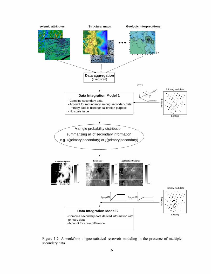
The sketch shown in Figure 1.2 demonstrates the overall workflow for reservoir modeling in

the presence of multiple secondary data. Exhaustiveness of the secondary data is an inherent

assumption. Qualitative maps from geologic interpretation should be converted into digitized

images. Data aggregation step is aimed at reducing the number of original secondary data by

removing irrelevant data, merging the relevant secondary data and both removing and merging.

The data aggregating step should be performed when too many secondary data, e.g., more than 6,

are initially prepared. Merged data will be treated as new secondary data for subsequent

integration. In the first integration step, the primary data are used only for calibrating the relation

between the primary and a set of secondary data. The spatial correlation of the primary data is

not considered in this step. No scale difference is assumed among the gridded secondary data.

As a result of the first step, several secondary data are converted into a single probability or

probability distribution term summarizing all secondary information. The relevance of the

secondary data to the primary data is fully accounted for in this step. For instance, higher

5

acoustic impedance may represent lower porosity or lower proportion of porous rock, and this

relation is quantified through probability distribution modeling. The second part in the overall

workflow (Figure 1.2) is to combine the primary data and the secondary data-derived

probabilities or probability distribution. Spatial cross correlation is modeled in this step.

Although the multiple secondary data are initially considered, a single calibrated secondary

variable is used hereafter because the first step integrates the multiple secondary data into a single

secondary derived variable. The effort of cross variogram modeling is considerably reduced; one

cross variogram is necessary regardless of the number of secondary data. The secondary data

themselves could be used as secondary variables for estimation and simulation without first

integration step. The secondary data calibration enters through the modeling of cross correlation

between the primary and secondary data. The relevance and redundancy of the secondary data

are implicitly modeled in cokriging (Journel and Huijbregts, 1978). Despite the flexibility of

cokriging, the two step modeling process is preferred because: (1) the inference of the cross

variogram becomes tedious in a direct use of secondary data, (2) any non-linear relations among

secondary data can be modeled in the secondary data integration, and (3) the integrated results

themselves may give useful information about the spatial variability of the primary variable

which could be used for reservoir management.

6

Figure 1.2: A workflow of geostatistical reservoir modeling in the presence of multiple secondary data.

-:fault

seismic attributes Structural maps Geologic interpretations

Data aggregation(if required)

Data Integration Model 1 - Combine secondary data - Account for redundancy among secondary data - Primary data is used for calibration purpose - No scale issue

Data Integration Model 2 - Combine secondary data derived information with primary data - Account for scale difference

A single probability distribution summarizing all of secondary information

e.g. p(primary|secondary) or f (primary|secondary)

0.0

1.0

Estimated prob Estimates

-2.0

0.0

2.0

Estimation Variance

γpri,sec(h)

0.0

1.0

Easting

Primary well data

Nor

thin

g

Easting

Primary well data

Nor

thin

g

secondary 1

secondary 2

primary

ρ

γpri,pri(h)

7

Cokriging is a spatial interpolator based on the spatial cross correlation; it is a well established

method for the second integration step of the workflow demonstrated in Figure 1.2. The scale

differences are accounted for by volume averaging covariances, and the redundancy of the

conditioning data are considered in the cokriging system of equations.

1.3 Problem Setting

This dissertation primarily focuses on the development of statistical approaches to integrate

secondary data. The necessity of an integrated probability that honors all of the given data is

universal in many scientific disciplines. Some previous works reached this goal by combining

probabilities that are individually calibrated with each data: see Winkler (1981), Bordley (1982)

and Clemen and Winkler (1999) in decision analysis, Lee et al. (1987) and Benediktsson and

Swain (1992) in image data fusion, and Journel (2002), Krishnan (2004), Krishnan et al. (2005)

and Polyakova and Journel (2007) in petroleum reservoir modeling. Individual conditional

probabilities, for example, p(sand|secondary data), can be the result of a physical equation or

statistical calibration. The univariate conditional probabilities are then combined leading to a

unified probability that is assumed to be jointly conditioned to all secondary data. The joint

relation modeling of the given data is not performed. In this approach, the important issue is to

reliably account for the redundancy or dependency among the secondary data. Data redundancy

is used as a term describing how much information originating from the diverse data are

redundant or overlapped. Redundancy could be alternatively interpreted as correlation between

data; high correlation means high redundancy and low correlation means less redundancy. As

pointed out by previous works, properly accounting for redundancy is crucial in the final

probability estimate (Benediktsson and Swain, 1992; Krishnan et al., 2004). Results could be

highly biased if the redundancy is not properly considered.

Another approach to integrate multiple secondary data is to model the joint relations directly

rather than calibrating and unifying the source-specific probabilities. In this approach, the

multivariate distribution is directly modeled and redundancy is implicitly accounted for through

the joint modeling. An external redundancy calibration, thus, is not required. Figure 1.3

demonstrates a brief sketch of two different methods to obtain the final probability conditioned to

all secondary data.

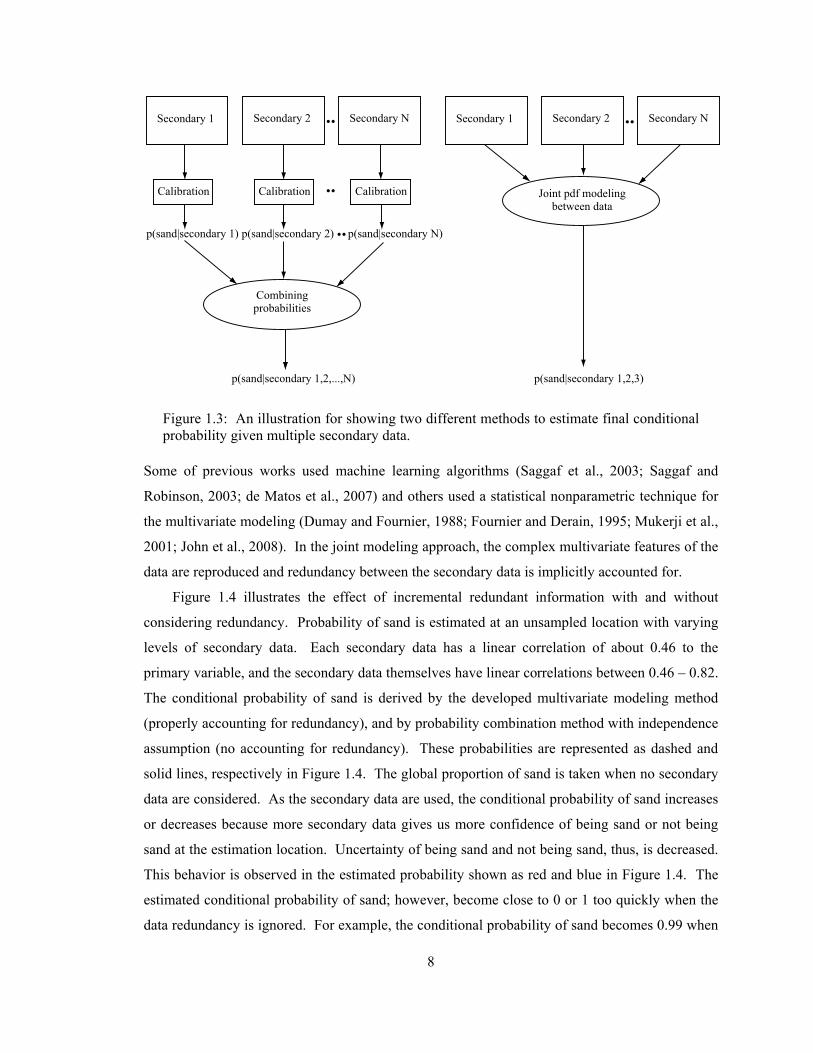
8

Figure 1.3: An illustration for showing two different methods to estimate final conditional probability given multiple secondary data.

Some of previous works used machine learning algorithms (Saggaf et al., 2003; Saggaf and

Robinson, 2003; de Matos et al., 2007) and others used a statistical nonparametric technique for

the multivariate modeling (Dumay and Fournier, 1988; Fournier and Derain, 1995; Mukerji et al.,

2001; John et al., 2008). In the joint modeling approach, the complex multivariate features of the

data are reproduced and redundancy between the secondary data is implicitly accounted for.

Figure 1.4 illustrates the effect of incremental redundant information with and without

considering redundancy. Probability of sand is estimated at an unsampled location with varying

levels of secondary data. Each secondary data has a linear correlation of about 0.46 to the

primary variable, and the secondary data themselves have linear correlations between 0.46 – 0.82.

The conditional probability of sand is derived by the developed multivariate modeling method

(properly accounting for redundancy), and by probability combination method with independence

assumption (no accounting for redundancy). These probabilities are represented as dashed and

solid lines, respectively in Figure 1.4. The global proportion of sand is taken when no secondary

data are considered. As the secondary data are used, the conditional probability of sand increases

or decreases because more secondary data gives us more confidence of being sand or not being

sand at the estimation location. Uncertainty of being sand and not being sand, thus, is decreased.

This behavior is observed in the estimated probability shown as red and blue in Figure 1.4. The

estimated conditional probability of sand; however, become close to 0 or 1 too quickly when the

data redundancy is ignored. For example, the conditional probability of sand becomes 0.99 when

Secondary 1 Secondary 2 Secondary N

Calibration Calibration Calibration

p(sand|secondary 1) p(sand|secondary 2) p(sand|secondary N)

p(sand|secondary 1,2,...,N) p(sand|secondary 1,2,3)

Combiningprobabilities

Secondary 1 Secondary 2 Secondary N

Joint pdf modelingbetween data

9

four secondary data are integrated without considering redundancy. This very high or very low

probability seems to be good in that the uncertainty is reduced in the resulting probability,

however, it has a risk of overestimation. The result with accounting for redundancy shows that

the probability is not as close to the extremes as the result without accounting for redundancy.

The increase in the estimated probability is not steep. The additional data becomes less helpful if

the added data are redundant. No or incorrectly accounting for redundancy leads to bias in the

estimated probability and it affects the final stochastic models.

Figure 1.4: An example illustrating incremental information impact on the probability estimate. Probabilities are estimated with and without accounting for data redundancy.

In the reservoir modeling studies, the use of multivariate density modeling is not new. This

dissertation advances a nonparametric multivariate analysis framework further; the joint relation

of the data is modeled in which different types of the data is not an issue and it is corrected by the

distribution constraints. The developed methodology leads to the joint distribution that ultimately

Number of secondary data

Correlatedsecondarydata

1

0

prob

(san

d)

Estimate without accounting forredundancy

Globalproportion ofsand

Estimate with accounting forredundancy

10

satisfies all axioms of probability distribution functions as well as the complex features among

the given data.

1.4 Dissertation Outline

Chapter 2 presents an overview of probabilistic modeling and fundamental geostatistical concepts.

Random function concepts and spatial variability are briefly introduced. Collocated cokriging

method is explained as a method to integrate primary well data and secondary derived results.

Debiasing with soft secondary data is addressed as a way to obtain representative global statistics.

Because the advanced debiasing technique with multiple soft secondary data is proposed in

Chapter 5, a key idea of debiasing is introduced in Chapter 2.

Chapter 3 introduces probability combination approaches for the secondary data integration.

The existing combination models are reviewed and some interesting points among them are

addressed. New weighted combination method, the Lamda-model, is developed and a key

contribution of the method is discussed. Some interesting features of the different combination

models are noted through a small 1-D example. The accuracy assessment criteria are introduced

in Chapter 3 that are used to evaluate the result through this dissertation.

Chapter 4 and 5 are involved in developing the multivariate density estimation technique to

the secondary data integration. In Chapter 4, the kernel density estimation method is introduced

as a nonparametric distribution modeling technique. Issues related to the choice of kernel

bandwidth and computational costs are explained. In the latter part of Chapter 4, marginality

constraints are introduced and how to impose them is discussed. An iterative marginal fitting

algorithm is proposed. The idea of the algorithm is to evaluate the extracted marginals from the

obtained joint distribution with the given reference marginals, and to correct the obtained

distribution by the amount of marginal differences. The convergence of the iteration is proved at

the end of the chapter. Chapter 5 presents application of the proposed multivariate analysis

framework to the facies modeling. Integrating multiple soft secondary data with varying scales

and integrating soft secondary and a geologic map are studied. Chapter 6 presents a derivation of

Bayesian updating in great details and proposes a new form of the updating equation. The

application of the multivariate modeling method to the Bayesian updating is presented with real

example.

Chapter 7 concludes the dissertation. The main contribution of this work, advantages and

disadvantages of the discussed methods are reviewed including possible future work.

11

Appendix A discusses the factorial kriging that is used to identify the spatial features or

factors based on scales. The technique can be used for filtering the unwanted noise or enhancing

the spatial features in the exhaustive secondary data before the secondary data integration. The

improved factorial kriging method is introduced in the appendix.

12

Chapter 2

Probabilistic Reservoir

Modeling

A probabilistic approach is preferentially adopted for numerical reservoir modeling because the

probabilistic model helps to describe the uncertainty in the constructed geologic model. At an

early stage of reservoir modeling, it is especially important to model the uncertainty associated

with the reservoir properties since this uncertainty could have a great impact on subsequent

reservoir modeling and the accuracy of reservoir forecasting. This chapter introduces

geostatistical theory, concepts and techniques that are used to quantify the uncertainty.

Geostatistical estimation and simulation methods are described briefly. One could also refer to

books on geostatistics for extensive discussions (Journel and Huigjbregts, 1978, Goovaerts, 1997,

Isaaks and Srivastava, 1989, Wackernagel, 2003).

2.1 Probabilistic Approach

Modeling the reservoir properties involves the uncertainty from the fact that the available data is

not exhaustive over the study domain. Let {z(uα), α=1,…,n} be the set of n measurements of

attribute z at n different locations. Samples are assumed to characterize the unknown population

over the domain A. A model is required to characterize the attribute z over the entire domain. A

model is a representation of the unknown reality. The reality may be deemed as spatial

distribution of facies, porosities, permeabilities, and fluid saturations in petroleum reservoir

modeling. A sequential modeling of reservoir properties is often followed. The facies rock types

13

are modeled first because they have first order impact on the distribution of other reservoir

properties. Porosities and permeabilities are then modeled on a by-facies basis.

A deterministic model associates a single estimated value z*(u) to each unknown value z(u).

A single estimate may rely on the physics that governs the phenomenon and thus the single value

is estimated without significant errors. The possibility of other potential states of reservoir

properties is neglected in a deterministic model. Instead of a single estimated value for each

unknown z(u), the probabilistic approach generates a set of possible with corresponding

probabilities. A probabilistic model quantitatively describes our uncertainty about the value by

probabilities.

Probabilistic models rely on data-driven statistics. For example, the spatial dependence of a

single attribute or the cross dependence of multiple attributes are inferred from the available

samples.

2.2 Geostatistical Techniques for Reservoir Modeling

Geostatistics is a branch of applied statistics dealing with spatial data. The goal of geostatistical

interpolation is to estimate the attribute of interest at unsampled locations and constructing the

probability distribution of the attribute. The constructed probability distribution characterizes the

local uncertainty. Stochastic heterogeneity modeling is based on these local uncertainty

distributions. Geostatistics has played an important role in building probabilistic models of

petroleum reservoirs. In particular, geostatistics is gaining applicability due to usefulness in

incorporating secondary data. Geostatistical techniques can build a probability distribution

conditioned to all primary and secondary information.

2.2.1 Random Function Concept

Geostatistics is largely based on the concept of a random function, whereby the set of unknown

values is regarded as a set of spatially dependent random variables. The local uncertainty about

the attribute value at any particular location u is modeled through the set of possible realizations

of the random variable at that location. The random function concept allows us to account for

structures in the spatial variation of the attribute. The set of realizations of the random function

models the uncertainty about the spatial distribution of the attribute over the entire area. The

location dependent random variable Z is denoted by Z(u). The random variable Z(u) is fully

14

characterized by its cumulative distribution function (cdf), which gives the probability that the

variable Z at location u is no greater than any given threshold z:

( ; ) Prob( ( ) )F z Z z= ≤u u

This cdf describes our uncertainty about the true value at the unsampled location u. Discrete

variables representing facies or rock type are denoted by S(u) and they take an integer code

s=1,…,K representing different types of facies. The probability of each category s=1,…,K to

prevail at location u is denoted as:

( ; ) Prob(S( ) ), 1,...,p s s s K= = =u u

Of course, the K probabilities p(u;s) must be non-negative and sum to one:

1

( ; ) 1K

s

p s=

=∑ u

A random function is defined as a set of usually dependent random variables Z(u), one for each

location u in the study area A, {Z(u),∀u∈A}. Any set of N locations uα, α=1,…,N corresponds a

vector of N random variables {Z(u1),…,Z(uα)} that is characterized by the N-variate of N-point

cdf:

1 1 1 1( ,..., ; ,..., ) Prob( ( ) ,..., ( ) )N N N NF z z Z z Z z= ≤ ≤u u u u

This joint cdf characterizes the joint uncertainty about the N values at N locations

{z(u1),…,z(uN)}. This spatial dependence defined by the multivariate cdf (equivalently pdf) is

referred to as spatial law of the random function Z(u). The joint uncertainty about the N

categorical values at N different locations can be similarly defined:

1 1 1 1( ,..., ; ,..., ) Prob( ( ) ,..., ( ) )N N N Np s s S s S s= = =u u u u

2.2.2 Measure of Spatial Dependence

One of the characteristics of earth science data is their spatial continuity. Whether the aim is the

estimation of unknown values at unsampled locations or simply the exploratory analysis of the

15

data set, the spatial continuity of the variable is an important factor. The foundation of

geostatistical algorithms, thus, is the description and inference of spatial continuity.

Covariance

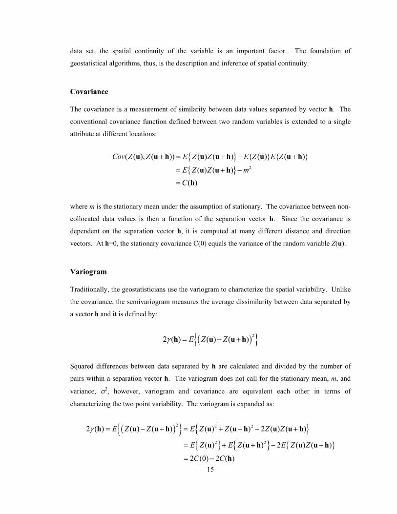
The covariance is a measurement of similarity between data values separated by vector h. The

conventional covariance function defined between two random variables is extended to a single

attribute at different locations:

{ }{ } 2

( ( ), ( )) ( ) ( ) { ( )} { ( )}

( ) ( )( )

Cov Z Z E Z Z E Z E Z

E Z Z mC

+ = + − +

= + −

=

u u h u u h u u h

u u hh

where m is the stationary mean under the assumption of stationary. The covariance between non-

collocated data values is then a function of the separation vector h. Since the covariance is

dependent on the separation vector h, it is computed at many different distance and direction

vectors. At h=0, the stationary covariance C(0) equals the variance of the random variable Z(u).

Variogram

Traditionally, the geostatisticians use the variogram to characterize the spatial variability. Unlike

the covariance, the semivariogram measures the average dissimilarity between data separated by

a vector h and it is defined by:

( ){ }22 ( ) ( ) ( )E Z Zγ = − +h u u h

Squared differences between data separated by h are calculated and divided by the number of

pairs within a separation vector h. The variogram does not call for the stationary mean, m, and

variance, σ2, however, variogram and covariance are equivalent each other in terms of

characterizing the two point variability. The variogram is expanded as:

( ){ } { }{ } { } { }

2 2 2

2 2

2 ( ) ( ) ( ) ( ) ( ) 2 ( ) ( )

( ) ( ) 2 ( ) ( )

2 (0) 2 ( )

E Z Z E Z Z Z Z

E Z E Z E Z Z

C C

γ = − + = + + − +

= + + − +

= −

h u u h u u h u u h

u u h u u h

h

16

This relation provides a key interpretation of variogram; (1) variogram and covariance have an

inverse relation, (2) at h=0, the variogram γ(0) is zero, (3) when h become large enough to have

no spatial correlation, then C(h) becomes zero leaving γ(h)=C(0)=σ2.

Indicator Variogram

Like the variogram of continuous random variable, spatial dependence of indicator variable can

be measured. Note that indicator variables are exclusive such as:

1, if facies occurs at

( ; )0, otherwise

sI s ⎧

= ⎨⎩

uu

Indicator covariance and variogram are calculated for the corresponding s=1,…,K as follows:

{ }

( ){ }

2

2

( ; ) I( ; )I( ; ) ( )and

( ; ) I( ; ) I( ; )

C s E s s p s

s E s sγ

= + −

= − +

h u u h

h u u h

p(s) is the stationary proportion of category s=1,…,K. Different categories surely show different

pattern of the spatial continuity so that the variogram, equivalently covariance of different facies

may be different. The indicator variogram and covariance have the following relation:

( ; ) (0; ) ( ; ), 1,...,s C s C s s Kγ = − =h h

2.2.3 Representative Statistics

Data are rarely collected with the goal of statistical representivity. Wells are often drilled in areas

with a greater probability of good reservoir quality. Core measurements are taken preferentially

from good quality reservoir rock. Physical inaccessibility also leads to data clustering. In almost

all cases, regular sampling is not practical. Naïve statistics from well samples could be biased.

The (unbiased) statistics, mean and variance, are needed as an input to the geostatistical

estimation and simulation. The importance of representative input parameters for geostatistical

simulation is well discussed in Pyrcz et al. (2006). Moreover, they provide a quick understanding

about the attribute being modeled over the domain: overall amount of porosities and oil saturation.

17

The mean computed from the unbiased distribution is a global estimate over the domain. The

mean is a naïve estimate at unsampled location without introducing any complicated local

estimation method.

Declustering

The original mean and standard deviation are calculated with the equal weights as:

2

1 1

1 1ˆ ˆ ˆand ( )n n

i ii i

m x x mn n

σ= =

= = −∑ ∑

where each datum xi, i=1,…,n has an equal impact for calculating the mean and standard

deviation. Declustering techniques assign each datum different weights, wi, i=1,…,n, based on its

closeness to surrounding data (Isaaks and Srivastava 1989; Deutsch and Journel, 1998).

Declustered mean and standard deviation are computed by:

2

1 1( )

n n

declustered i i declustered i i declusteredi i

m w x and w x mσ= =

= = −∑ ∑

where weights wi are greater than 0 and add to 1. Cell declustering methods computes the

weights based on the number of samples falling within the given cells (Deutsch, 2002).

Polygonal method calculates the weights based on the construction of polygons of influence

about each of the sample data (Isaaks and Srivastava, 1987).

Declustering with Soft Secondary Data

Declustering with the soft secondary data is another method to correct a biased distribution of a

primary variable being predicted. It assumes that the soft secondary data is representative of the

entire area of interest, and an understanding of the relationship between the primary and soft

secondary data. The underlying relation could be either linear or non-linear. The debiased

distribution of the primary variable could be obtained by numerical integral of the conditional

distribution over the range of all secondary data:

( ) ( | ) ( )Debiasedf z f z f d= ∫

y

y y y

18

where z and y are random variables of the primary and secondary data. f(z|y) is a conditional

distribution of the primary given the secondary data. In Chapter 5, debiasing technique using the

multivariate modeling framework is explained.

2.2.4 Geostatistical Estimation Algorithms

Kriging is a well-established methodology that provides the best linear unbiased estimate and its

variance at the unsampled locations. In theory, kriging is a statistically optimal interpolator in the

sense that it minimizes estimation variance when the covariance or variogram is known and under

the assumption of the stationarity.

Accounting for a Single Variable

Consider the problem of estimating the value of a continuous attribute z at an unsampled location

u using z-data available within the chosen area A. Most kriging estimators are linear combination

of the nearby conditioning data {z(uα), α=1,…n}. The kriged estimate is written:

*

1

( ) ( )[ ( ) ]n

Z m Z mα αα

λ=

− = −∑u u u

where n is the number of nearby data Z(uα) and λ(uα) are kriging weights assigned to datum Z(uα)

at the corresponding location uα. m is the expectation of random variable Z(u) being assumed

stationary. n is the number of associated nearby data to estimate Z(u) at unsampled location.

Solving the kriging equation is a process to achieve the kriging weights. Least square estimation

allows one to define the error variance between the estimate Z*(u) and the unknown true value

Z(u):

2 * 2( ) {( ( ) ( )) }error E Z Zσ = −u u u

The system of simple kriging equations is derived by minimizing the error variance as follows

(Goovaerts, 1997):

1

( ) ( ) ( ) 1,...,n

C C nβ α β αβ

λ α=

− = − =∑ u u u u u

19

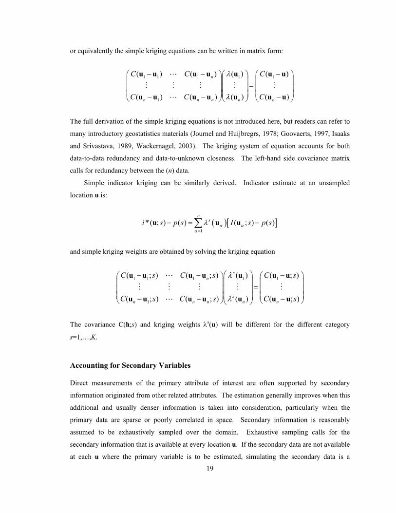
or equivalently the simple kriging equations can be written in matrix form:

1 1 1 1 1

1

( ) ( ) ( ) ( )

( ) ( ) ( ) ( )

n

n n n n n

C C C

C C C

λ

λ

− − −⎛ ⎞⎛ ⎞ ⎛ ⎞⎜ ⎟⎜ ⎟ ⎜ ⎟=⎜ ⎟⎜ ⎟ ⎜ ⎟⎜ ⎟⎜ ⎟ ⎜ ⎟− − −⎝ ⎠⎝ ⎠ ⎝ ⎠

u u u u u u u

u u u u u u u

The full derivation of the simple kriging equations is not introduced here, but readers can refer to

many introductory geostatistics materials (Journel and Huijbregrs, 1978; Goovaerts, 1997, Isaaks

and Srivastava, 1989, Wackernagel, 2003). The kriging system of equation accounts for both

data-to-data redundancy and data-to-unknown closeness. The left-hand side covariance matrix

calls for redundancy between the (n) data.

Simple indicator kriging can be similarly derived. Indicator estimate at an unsampled

location u is:

( )[ ]1

*( ; ) ( ) ( ; ) ( )n

si s p s I s p sα αα

λ=

− = −∑u u u

and simple kriging weights are obtained by solving the kriging equation

1 1 1 1 1

1

( ; ) ( ; ) ( ) ( ; )

( ; ) ( ; ) ( ) ( ; )

sn

sn n n n n

C s C s C s

C s C s C s

λ

λ

⎛ ⎞− − −⎛ ⎞ ⎛ ⎞⎜ ⎟⎜ ⎟ ⎜ ⎟=⎜ ⎟⎜ ⎟ ⎜ ⎟

⎜ ⎟ ⎜ ⎟⎜ ⎟− − −⎝ ⎠ ⎝ ⎠⎝ ⎠

u u u u u u u

u u u u u u u

The covariance C(h;s) and kriging weights λs(u) will be different for the different category

s=1,…,K.

Accounting for Secondary Variables

Direct measurements of the primary attribute of interest are often supported by secondary

information originated from other related attributes. The estimation generally improves when this

additional and usually denser information is taken into consideration, particularly when the

primary data are sparse or poorly correlated in space. Secondary information is reasonably

assumed to be exhaustively sampled over the domain. Exhaustive sampling calls for the

secondary information that is available at every location u. If the secondary data are not available

at each u where the primary variable is to be estimated, simulating the secondary data is a

20

reasonable approximation to complete the exhaustiveness of the secondary information (Almeida

and Journel, 1994).

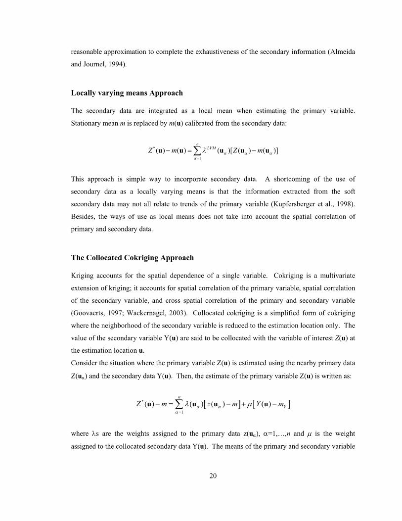
Locally varying means Approach

The secondary data are integrated as a local mean when estimating the primary variable.

Stationary mean m is replaced by m(u) calibrated from the secondary data:

*

1( ) ( ) ( )[ ( ) ( )]

nLVMZ m Z mα α α

α

λ=

− = −∑u u u u u

This approach is simple way to incorporate secondary data. A shortcoming of the use of

secondary data as a locally varying means is that the information extracted from the soft

secondary data may not all relate to trends of the primary variable (Kupfersberger et al., 1998).

Besides, the ways of use as local means does not take into account the spatial correlation of

primary and secondary data.

The Collocated Cokriging Approach

Kriging accounts for the spatial dependence of a single variable. Cokriging is a multivariate

extension of kriging; it accounts for spatial correlation of the primary variable, spatial correlation

of the secondary variable, and cross spatial correlation of the primary and secondary variable

(Goovaerts, 1997; Wackernagel, 2003). Collocated cokriging is a simplified form of cokriging

where the neighborhood of the secondary variable is reduced to the estimation location only. The

value of the secondary variable Y(u) are said to be collocated with the variable of interest Z(u) at

the estimation location u.

Consider the situation where the primary variable Z(u) is estimated using the nearby primary data

Z(uα) and the secondary data Y(u). Then, the estimate of the primary variable Z(u) is written as:

[ ] [ ]*

1( ) ( ) ( ) ( )

n

YZ m z m Y mα αα

λ μ=

− = − + −∑u u u u

where λs are the weights assigned to the primary data z(uα), α=1,…,n and μ is the weight

assigned to the collocated secondary data Y(u). The means of the primary and secondary variable

21

are denoted by m and mY, respectively. The cokriging equation is derived by minimizing the error

variance:

{ }2 * 2( ) ( ( ) ( ))error E Z Zσ = −u u u

The full system of collocated cokriging equation is followed by in a matrix form:

1 1 1 1 11

1 1

1

( ) ( ) ( ) ( )( )

( ) ( ) ( ) ( )( )( ) ( ) (0) (0)( )

ZZ ZZ a ZY ZZ

ZZ ZZ a ZY ZZ

YZ YZ YY YZ

C C C c

C C C cC C C c

α α α α

α

λ

λμ

− − − −⎡ ⎤ ⎡ ⎤⎡ ⎤⎢ ⎥ ⎢ ⎥⎢ ⎥⎢ ⎥ ⎢ ⎥⎢ ⎥ =⎢ ⎥ ⎢ ⎥⎢ ⎥− − − −⎢ ⎥ ⎢ ⎥⎢ ⎥− − ⎣ ⎦ ⎣ ⎦⎣ ⎦

u u u u u u u uu

u u u u u u u uuu u u u u

where the covariance Czz is the left hand matrix of the simple kriging system of Z(u) and cZZ is

the corresponding right hand side covariance vector. The vector cYZ contains the cross

covariances between the n samples of Z and the estimation location u with its collocated

secondary value Y(u). CYY(0) is the variance of Y and cYZ(0) is the cross-covariance between the

collocated Z(u) and Y(u).

The cross covariance cYZ is usually approximated using the Markov model (Journel, 1999).

The collocated cokriging system of equations can be written using the Markov model for the

cross covariance:

1 1 1 1 11

1 1

1

( ) ( ) ( ) ( )( )

( ) ( ) ( ) ( )( )( ) ( ) (0) (0)( )

ZZ ZZ a ZZ ZZ

ZZ ZZ a ZZ ZZ

ZZ ZZ YY YZ

C C bC c

C C bC cbC bC C c

α α α α

α

λ

λμ

− − − −⎡ ⎤ ⎡ ⎤⎡ ⎤⎢ ⎥ ⎢ ⎥⎢ ⎥⎢ ⎥ ⎢ ⎥⎢ ⎥ =⎢ ⎥ ⎢ ⎥⎢ ⎥− − − −⎢ ⎥ ⎢ ⎥⎢ ⎥− − ⎣ ⎦ ⎣ ⎦⎣ ⎦

u u u u u u u uu

u u u u u u u uuu u u u u

where b = (0) (0)(0)

ZYZ

Y

CC

ρ⎛ ⎞

⋅⎜ ⎟⎝ ⎠

, ρYZ(0) is the correlation coefficient of the collocated Z

and Y. The collocated cokriging approach with the Markov model only requires the primary

variable covariance function, the variance of the secondary data and the correlation coefficient

between the primary and the secondary data. Retaining the collocated secondary data may not

affect the estimates, however, the cokriging variances are often overestimated which can cause a

serious problem in a sequential simulation (Deutsch, 2002).

22

The Bayesian Updating Approach

The collocated cokriging with the Markov model is equivalent to the Bayesian expression of the

cokriging estimate (Doyen, 1996; Chiles and Delfiner, 1999). For example, the cokriging

estimate and variance are the mean and variance of the probability distribution conditioned to the

nearby primary and the collocated secondary data:

11

( ( ) | ( ),..., ( ))( ( ) | ( ),..., ( ), ( )) ( ( )) ( ( ) | ( )) ,( ( ))

f z z zf z z z y f z f y z C Af z

αα = ⋅ ∈

u u uu u u u u u u uu

where the C is the normalizing term and it does not affect the mean and variance of the

probability distribution. The conditional independence assumption is made to separate the

f(z(u)|z(u1),…, z(uα),y(u) into the product of f(z(u)|z(u1),…,z(uα)) and f(y(u)|z(u)). The

conditional probability function f(y(u)|z(u)) is a likelihood because the z(u) is the unknown and

the y(u) is the given known value. It is re-expressed as:

( ( ) | ( ))( ( ) | ( )) ( ( ))

( ( ))f z yf y z f y

f z=

u uu u uu

and then the following Bayesian updating equation can be derived,

11

( ( ) | ( ), ..., ( )) ( ( ) | ( ))( ( ) | ( ), ..., ( ), ( )) ( ( )) ,( ( )) ( ( ))

f z z z f z yf z z z y f z C Af z f z

αα = ⋅ ∈

u u u u uu u u u u uu u

where the probability distribution functions that are not related to the z(u) are absorbed in the

normalizing term C. Finally, the conditional probability function of interest is shown as the

production of two probability functions conditioned to the set of the primary data z(u1),…,z(uα)

and the collocated secondary data y(u), and the univariate probability function of z(u), f(z(u)).

Under the stationarity of the z(u), the f(z(u)) is replaced as the global pdf f(z). The simple kriging

estimate and estimation variance are the mean and variance of f(z(u)|z(u1),…,z(uα)) under the

multiGaussian assumption among z(u),z(u1),…,z(uα) (Verly, 1983). The mean and variance of

f(z(u)|y(u)) can be simplified using the correlation coefficient between Z and Y. Thus, the final

estimate and estimation variance of z(u) that are the mean and variance of the conditional

probability function above can be obtained by the simple kriging estimate and estimation variance,

linear correlation coefficient, and the global mean and variance. Similarly, the Bayesian

expression for the categorical variable can be shown as,

23

11

( ( ) | ( ),..., ( )) ( ( ) | ( ))( ( ) | ( ),..., ( ), ( )) ( ) ,( ) ( )

p i i i p i yp i i i y p s C Ap s p s

αα = ⋅ ∈

u u u u uu u u u u

where the conditioning data i(uα), α=1,…,n are indicators. These Bayesian expressions are often

useful to understand clearly: they decompose the final conditional probability of interest into the

primary variable-related and the secondary variable-related terms.

2.2.5 Geostatistical Simulation

Geostatistical simulation adds a random component to the kriging estimate to reproduce the

realistic heterogeneity of the reservoir. Multiple realizations of heterogeneity are obtained from

randomly drawing different random components. These realizations can provide an assessment

of the uncertainty about the reservoir properties being modeled. Motivations for the simulation

are in two aspects. First of all, geostatistical simulation corrects the smoothness in the kriging

estimates. Kriging estimates are theoretically right, however, it smears out the high frequency

features (Wackernagel, 2003). Secondly, geostatistical simulation allows the calculation of the

joint uncertainty when several locations are considered together. Quantifying the joint

uncertainty is very important to reflect the geologic heterogeneity and critical to the reservoir

performance.

There are many approaches that can be used for the geostatistical simulation. The most

popular and simplest technique is the sequential Gaussian simulation for the continuous variable,

and sequential indicator simulation for the categorical variable. Sequential simulation is based on

the application of the Bayes law to decompose the multivariate distribution at different locations

into a series of conditional distributions for each location. The random component that corrects

kriging smoothness is drawn from the local probability distributions that are obtained from

kriging or cokriging. Procedures for sequential simulation are well described in Goovaerts (1997),

Deutsch (2002) and other standard geostatistics references.

2.3 Discussions

Fundamental concepts of geostatistics are briefly reviewed. The goal of the geostatistical

estimation algorithm is to build the local conditional probability distribution. Geostatistical

simulation describes the uncertainty of the underlying geologic variability based on the local

conditional distribution.

24

Cokriging is a well-established technique to build local distribution using the primary and

the secondary data. Tedious efforts for cross variogram modeling required for the cokriging can

be eliminated using the Markov assumption, and thus, the collocated cokriging with the Markov

model is widely used in practice.

The collocated cokriging estimate and Bayesian expressions are exactly equivalent.

However, Bayesian form is easier to understand how different distributions conditioned to

different data are combined leading to a final conditional distribution.

25

Chapter 3

Probability Combination

Schemes

This chapter presents probability combination methods for calculating the probability of a

primary attribute conditioned to multiple secondary data. These approaches combine conditional

probabilities derived from calibrating each secondary data, possibly with different calibration

techniques. Probability combination schemes (PCS in short) have been developed independently

in many research areas in order to find a unified probability from using several single source

derived probabilities (Winkler, 1981; Bordley, 1982; Lee et al., 1987; Benediktsson and Swain

1992; Clemen and Winkler, 1999). Probability combination schemes were recently applied in

reservoir modeling for an improved reservoir characterization using various secondary data

(Krishnan, 2004; Liu et al., 2004; Polyakova and Journel, 2007; Castro et al., 2005).

The main goal of PCS is to approximate the target conditional probability through linking

the individual probabilities that are computed using individual data sources. The use of PCS is

very attractive when the conditional probability p(s|D1,…,Dm) where s is facies or rock type and

(D1,…,Dm) are m secondary data, is hard to obtain or even impossible to model in a coherent

manner. Alternatively, there may be no access to the data themselves directly but only access to

the calibrated probabilities p(s|Di). For example, the data Di for i=1,…,m can be seismic

attributes, trends from geology, analogue data and expert knowledge. PCS approaches

approximate the joint probability by linking probabilities individually calibrated with data Di,

i=1,…,m subject to the primary variable s. Inference of individual probabilities p(s|Di) is not an

interest. Each data could have a different calibration method based on statistical modeling,

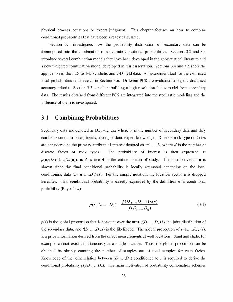
26

physical process equations or expert judgment. This chapter focuses on how to combine

conditional probabilities that have been already calculated.

Section 3.1 investigates how the probability distribution of secondary data can be

decomposed into the combination of univariate conditional probabilities. Sections 3.2 and 3.3

introduce several combination models that have been developed in the geostatistical literature and

a new weighted combination model developed in this dissertation. Sections 3.4 and 3.5 show the

application of the PCS to 1-D synthetic and 2-D field data. An assessment tool for the estimated

local probabilities is discussed in Section 3.6. Different PCS are evaluated using the discussed

accuracy criteria. Section 3.7 considers building a high resolution facies model from secondary

data. The results obtained from different PCS are integrated into the stochastic modeling and the

influence of them is investigated.

3.1 Combining Probabilities

Secondary data are denoted as Di, i=1,…,m where m is the number of secondary data and they

can be seismic attributes, trends, analogue data, expert knowledge. Discrete rock type or facies

are considered as the primary attribute of interest denoted as s=1,…,K, where K is the number of

discrete facies or rock types. The probability of interest is then expressed as

p(u;s|D1(u)…,Dm(u)), u∈A where A is the entire domain of study. The location vector u is

shown since the final conditional probability is locally estimated depending on the local

conditioning data (D1(u),…,Dm(u)). For the simple notation, the location vector u is dropped

hereafter. This conditional probability is exactly expanded by the definition of a conditional

probability (Bayes law):

11

1

( ,..., | ) ( )( | ,..., )( ,..., )

mm

m

f D D s p sp s D Df D D

= (3-1)

p(s) is the global proportion that is constant over the area, f(D1,…,Dm) is the joint distribution of

the secondary data, and f(D1,…,Dm|s) is the likelihood. The global proportion of s=1,…,K, p(s),

is a prior information derived from the direct measurements at well locations. Sand and shale, for

example, cannot exist simultaneously at a single location. Thus, the global proportion can be

obtained by simply counting the number of samples out of total samples for each facies.

Knowledge of the joint relation between (D1,…,Dm) conditioned to s is required to derive the

conditional probability p(s|D1,…,Dm). The main motivation of probability combination schemes

27

is based on the unavailability of the joint distribution. Some assumptions are required to

approximate the conditional probability without modeling the joint probability distribution.

3.2 Simple Combination Models

A simple combination model assumes the data (D1,…,Dm) are conditionally independent. These

assumptions greatly simplify the process of calculating the final conditional probability at the

possible expense of a loss in accuracy of the probability estimate.

3.2.1 Conditional Independence Model

A less strict assumption is that the secondary data (D1,…,Dm) are independent conditioned to the

possible outcomes of the primary variable s=1,…,K. The conditional independence assumption

decomposes the joint probability f(D1,…,Dm|s) into the linear product of f(D1|s)×⋅⋅⋅×f(Dm|s).

Equation (3-1) is expanded as:

1

1

1

1

1

11

1

( | ,..., )( ,..., | ) ( )

( ,..., )( | ) ( | ) ( )

( ,..., )( | ) ( ) ( )( | ) ( )

( ) ( ) ( ,..., )

m

m

m

m

m

m m

m

p s D Df D D s p s

f D Df D s f D s p s

f D Dp s D f D f Dp s D p s

p s p s f D D

=

⋅⋅⋅=

⋅⋅ ⋅= ⋅⋅⋅

(3-2)

Because f(D1)×⋅⋅⋅×f(Dm)/f(D1,…,Dm) does not affect the final conditional probability

p(s|D1,…,Dm), it is collapsed into a normalizing term C:

11

( | )( | )( | , ..., ) ( )( ) ( )

mm

p s Dp s Dp s D D p s Cp s p s

= ⋅⋅ ⋅ (3-3)

Thus, the conditional probability p(s|D1,…,Dm) can be now approximated by the product of

probability ratios p(s|Di)/p(s), i=1,…,m and the global proportion p(s). For example, consider

three data seen as three different secondary data D1, D2 and D3 informing about the probability of

facies s=1,2 and 3 occurring. The global proportion and individual probability of facies are

illustrated in the table below,

28

p(s) p(s|D1) p(s|D2) p(s|D1,D2)

s=1 0.2 0.3 0.45 0.535

s=2 0.3 0.4 0.35 0.37

s=3 0.5 0.3 0.2 0.095

marginal 1 1 1 1

Note that each data assess the possibility of facies s=1, 2 at higher probability than the global

proportion, and that of facies s=3 at lower probability than the global proportion. The combined

probability is shown in the last column. The marginal sum of p(s|D1,D2) amounts to 1 because of

standardization. An interesting aspect of the combined probabilities is that they become larger or

smaller if the individual conditional probabilities are all larger or smaller than the global

proportion. This phenomenon of pushing the resulting probability toward to the extremes is

called non-convexity and this property is discussed more in sections 3.4 and 3.5 through

examples. Note that the probabilities shown in the table above are arbitrarily injected merely to

see the non-convexity of the combined probability.

3.2.2 Permanence of Ratios Model (PR model)

Journel (2002) developed a permanence of ratios (PR) model that approximates the probability

assuming that ratios of probability increments from different data sources are constant. Although

the PR model was independently developed in the geostatistics literature, it is also used in other

fields (Pearl, 1988; Friedman et al., 1997). The principle of PR is that ratios are more stable than

the increments themselves (Journel, 2002). Consider the ratios of probability of s:

( ) [0, ]( )

p sap s

= ∈ ∞

what can be interpreted as the probability distance to s occurring, e.g. if p(s)=1 (s certainly occurs)

⇒ a=0 (distance) and if p(s)=0 (s certainly does not occur)⇒ a=∞ (infinite distance). Note that

p( s ) is the probability of not s that is, 1− p(s). Similarly, the probability distances to s given the

data D1 and D2 are, respectively:

29

1 21 2

1 2

( | ) ( | )[0, ] and [0, ]( | ) ( | )

p s D p s Dd dp s D p s D

= ∈ ∞ = ∈ ∞

The probability distance to be estimated is then:

1 2

1 2

( | , ) [0, ]( | , )

p s D Dxp s D D

= ∈ ∞

Permanence of ratios assumes that the incremental contribution of D2 to an event s with

knowledge of D1 is the same as that of D2 to an event s without knowing D1. This assumption is

expressed as the following equality:

2

1

x dd a

=

The ratio x/d1 represents the contribution of data D2 knowing D1; if data D2 has no contribution to

s then the ratio becomes unity. The ratio d2/a represents the contribution of data D2 to s. The

conditional probability of interest p(s|D1,D2) is now derived from the PR model (denoted as pPR):

1 21 2 1 2

1 2

1 ( )1 ( )( | , ) [0,1]

1 1 ( | ) 1 ( | )1 ( )( ) ( | ) ( | )

PR

p sa p sp s D D

x a d d p s D p s Dp sp s p s D p s D

−

= = = ∈+ + ⎛ ⎞⎛ ⎞− −−

+ ⎜ ⎟⎜ ⎟⎝ ⎠⎝ ⎠

This equation can be generalized with many conditioning data (D1,…,Dm) by:

1

1 1

1

1 ( )( )

( | ,..., ) [0,1]1 ( | )1 ( )

( ) ( | )

m

PR m m mi

i i

p sp s

p s D Dp s Dp s

p s p s D

−

−

=

⎛ ⎞−⎜ ⎟⎝ ⎠= ∈

⎛ ⎞⎛ ⎞ −−+ ⎜ ⎟⎜ ⎟

⎝ ⎠ ⎝ ⎠∏

(3-4)

The estimated probability pPR meets the closure condition and non negativity regardless of

number of conditioning data Di, i=1,…,m. The PR model, however, is limited to binary variable

modeling. For instance, consider that s can take three outcomes such as sand (coded as s=1),

intermediate sand (coded as s=2) and shale (coded as s=3). Arbitrary p(s), p(s|D1) and p(s|D2),

30

s=1,2,3 are shown in the table below. The combined probability using the PR model is indicated

in the right column.

p(s) p(s|D1) p(s|D2) pPR(s|D1,D2)

s=1 0.2 0.3 0.45 0.584

s=2 0.3 0.4 0.35 0.456

s=3 0.5 0.3 0.2 0.097

marginal 1 1 1 1.136

The marginal sum of pPR(s|D1,D2) does not equal to 1 as shown in the lower right corner. This

violation of the closure condition is not limited to this particular numeric example.

The assumption made in the PR model is the same as the independence assumption of

(D1,…,Dm) conditioned to primary variable s. Equivalence of the PR model and conditional

independence is proved for the binary case. As shown in Equation (3-3), the conditional

independence obtains the probability of interest as (denoted as pCI):

11

1

( | )( | )( | ,..., ) ( )( ) ( )

( | )( ) [0,1]( )

mCI m

mi

i

p s Dp s Dp s D D p s Cp s p s

p s Dp s Cp s=

= ×⋅⋅⋅×

⎛ ⎞= ∈⎜ ⎟

⎝ ⎠∏

(3-5)

C is the unknown normalizing term. By enforcing the closure condition, the C term will be

removed by standardization:

31

( )1

1

1 1

1

1

( | )( )( )

( | ,..., )( | ) 1 ( | )( ) 1 ( )

( ) 1 ( )

11 ( | )1 ( ) ( )1

( ) 1 ( ) ( | )

1 ( )( )

1 ( )( )

mi

iCI m m m

i i

i i

m mi

i i

m

p s Dp s Cp s

p s D Dp s D p s Dp s C p s C

p s p s

p s Dp s p sp s p s p s D

p sp s

p sp s

=

= =

=

−

⎛ ⎞⎜ ⎟⎝ ⎠=

⎛ ⎞ ⎛ ⎞−+ −⎜ ⎟ ⎜ ⎟−⎝ ⎠ ⎝ ⎠

=⎛ ⎞⎛ ⎞⎛ ⎞ −−+ ⎜ ⎟⎜ ⎟⎜ ⎟−⎝ ⎠⎝ ⎠ ⎝ ⎠

⎛ ⎞−⎜ ⎟⎝ ⎠=

⎛ −

∏

∏ ∏

∏

11

1

( | ,..., ) [0,1]1 ( | )

( | )

PR mm mi

i i

p s D Dp s D

p s D

−

=

= ∈⎛ ⎞⎞ −

+ ⎜ ⎟⎜ ⎟⎝ ⎠ ⎝ ⎠

∏

This equivalence holds for the binary case. The PR model is not strictly valid when more than

two categories are considered. Instead, conditional independence can be used for any case

because it enforces the closure condition, for example when three categories are considered with

s=1,2, and 3:

1

1

1 1 1

( | ,..., )

( | )( )( )

[0,1]( | ) ( ' | ) ( '' | )( ) ( ') ( '')

( ) ( ') ( '')

CI m

mi

im m m

i i i

i i i

p s D D

p s Dp sp s

p s D p s D p s Dp s p s p sp s p s p s

=

= = =

=

⎛ ⎞⎜ ⎟⎝ ⎠ ∈

⎛ ⎞ ⎛ ⎞ ⎛ ⎞+ +⎜ ⎟ ⎜ ⎟ ⎜ ⎟

⎝ ⎠ ⎝ ⎠ ⎝ ⎠

∏

∏ ∏ ∏

(3-6)

where s′≠s′′≠s=1,2,3. The conditional independence model should be used in the case of multiple

categories.

The permanence of ratios and conditional independence models assume independence

among the secondary data conditioned to the primary attribute of interest. By adopting this

independence assumption, the task of combining probabilities is simplified into the product of

individual probabilities, p(s|Di) for i=1,…,m. Correlation or redundancy among the data is simply

ignored for the convenience of calculation. In some cases, however, those simple models could

introduce a serious bias in the resulting probability. Advanced probability combination methods

to account for data redundancy are discussed next.

32

3.3 Weighted Combination Model

Ignoring the data redundancy assumes all secondary data are uncorrelated with little information

overlap. This could make the resulting combined probability close to an extreme probability of 0

or 1 as shown in the introductory example in Figure 1.4. The property of falling outside the input

probability p(s) and p(s|Di), is called non-convex property. This non-convexity is desirable if the

data are not highly correlated with each other, but may not be desirable if the data are highly

correlated. In reality, the secondary data are correlated to some degree through the primary

variable being modeled.

Weighted combination models were developed to mitigate the effect of the independence

assumption by adjusting the relative influence of the secondary data. If the data (D1,…,Dm) are

redundant with moderate to high degree then their influence should be reduced because some of

the data largely explain the rest of data. The tau model is one example proposed by Journel

(2002). In the tau model, probability ratios are weighted by exponents denoted as τ. Varying the

τ values adjusts the impact of individual probabilities on the combined probability. Krishanan

(2008) derived analytical solutions of these weight parameters that exactly quantify the

redundancy of the given conditioning data. Although the solution is analytically derived, they are

case dependent without general form. Another model, the Lamda model, is developed in this

thesis. Power weights are imposed on the individual probability ratios, but the calibration is

different from the Tau model. Weighted combination models can be expressed with data specific

power weights (w1,…,wm):

1

1 1( | ,..., ) ( | )( | ) ...( ) ( ) ( )

mw w

m mp s D D p s Dp s D Cp s p s p s

⎛ ⎞ ⎛ ⎞= × ×⎜ ⎟ ⎜ ⎟⎝ ⎠ ⎝ ⎠

(3-7)

Equation (3-7) reverts to the conditional independence model when the data specific weights wi

are all 1. If the weights are not unity, the contribution of p(s|Di) is adjusted. The degree of

adjustment depends on the data redundancy.

3.3.1 Tau model

The Tau model is one example of weighted combination methods. If the weights wi in Equation

(3-7) are replaced by τi and the binary category is considered then the weighted combination

33

shown in Equation (3-7) is referred to as the Tau model. Equivalence between Equation (3-7)

with the replaced τi and the original form of the Tau model is proved in the end of this section.

The Tau model is expressed as by Journel (2002):

2

1

dxd a

τ⎛ ⎞= ⎜ ⎟⎝ ⎠

(3-8)

where τ is dependent on the relation between D1 and D2. The range of the parameter τ is within

[0,∞] to make the resulting probability p(s|D1,D2) in [0,1]. By introducing this power weight, the

ratio (d2/a) will be increased or decreased. Equation (3-8) can be generalized with many data

(D1,…,Dm) by introducing successive m weights:

1 1

i im mi i

i i

d dx x aa a a

τ τ

= =

⎛ ⎞ ⎛ ⎞= ⇔ =⎜ ⎟ ⎜ ⎟⎝ ⎠ ⎝ ⎠

∏ ∏ (3-9)

The important factor in the Tau model is τi for i=1,…,m that can be in [−∞ ,∞ ] (Krishnan, 2008).

The probability of interest is derived from Equation (3-9) as:

1

1

1

1 1

1

1 ( | )1 ( | )1 ( | ,..., ) ( | )( | )1 ( )

1 ( ) 1 ( )( | ,..., ) ( )( ) ( )

i

m

mi

i

m

m m

m

dx aa

p s Dp s Dp s D D p s Dp s Dp s

p s p sp s D D p sp s p s

τ

ττ

=

⎛ ⎞= ⇔⎜ ⎟⎝ ⎠

−− ⎛ ⎞⎛ ⎞⎜ ⎟⎜ ⎟− − ⎜ ⎟⎜ ⎟= ×⋅⋅⋅×

− −⎜ ⎟⎜ ⎟⎜ ⎟ ⎜ ⎟⎝ ⎠ ⎝ ⎠

∏

And,

111

1

1( | ,..., )1 ( | )1 ( | )

( | )( | )1 ( )1 1 ( ) 1 ( )( )( ) ( )

mmm

m

p s D Dp s Dp s D

p s Dp s Dp sp s p sp s

p s p s

ττ=−− ⎛ ⎞⎛ ⎞

⎜ ⎟⎜ ⎟− ⎜ ⎟⎜ ⎟+ ×⋅⋅⋅×− −⎜ ⎟⎜ ⎟

⎜ ⎟ ⎜ ⎟⎝ ⎠ ⎝ ⎠

1

1

1

1

1 ( | )1 ( | )1 ( ) ( ) ( )1( ) ( | ) 1 ( ) ( | ) 1 ( )

m

m

m

p s Dp s Dp s p s p sp s p s D p s p s D p s

ττ=⎛ ⎞⎛ ⎞ −−−+ × ×⋅⋅ ⋅× ×⎜ ⎟⎜ ⎟− −⎝ ⎠ ⎝ ⎠

34

11 1

1

1

1 ( | )1 ( | )1 ( ) ( )1( ) 1 ( ) ( | ) ( | )

m

mii m

m

p s Dp s Dp s p sp s p s p s D p s D

τττ=

=∑ ⎛ ⎞⎛ ⎞⎛ ⎞ −−−

+ ×⋅⋅ ⋅× ⎜ ⎟⎜ ⎟⎜ ⎟−⎝ ⎠ ⎝ ⎠ ⎝ ⎠

1

11

1

1 ( ) ( )( ) 1 ( )

1 ( | )1( | )

1 ( ) ( )( ) 1 ( )

m

ii

i

m

ii

mi

i i

p s p sp s p s

p s Dp s D

p s p sp s p s

τ

τ

τ

=

==

∑⎛ ⎞−⎜ ⎟−⎝ ⎠=

⎛ ⎞−+ ⎜ ⎟

∑ ⎝ ⎠⎛ ⎞−⎜ ⎟−⎝ ⎠

∏

The above equation is rearranged:

1

1

1

1

( ) 1 ( )1 ( ) ( )

( | ,..., ) [0,1]1 ( | )( ) 1 ( )

1 ( ) ( ) ( | )

m

ii

m

iii

Tau mm

i

i i

p s p sp s p s

p s D Dp s Dp s p s

p s p s p s D

τ

ττ

=

=

=

∑⎛ ⎞−⎜ ⎟− ⎝ ⎠= ∈∑ ⎛ ⎞⎛ ⎞ −−

+ ⎜ ⎟⎜ ⎟− ⎝ ⎠ ⎝ ⎠∏

(3-10)

which is the Tau model that approximates the conditional probability of interest from the

weighted combination of individual probabilities. Similar to the PR model, the Tau model

ensures the closure condition only for the binary case of primary variable s. The closure

condition of pTau(s|D1,…,Dm) over s=1,…,K is not guaranteed. Equation (3-10) is a standardized

expression of Equation (3-7) using the complementary probability 1−p(s|Di) and 1−p(s), which

removes the constant term C as:

( )

1

11

1

1 1

( | )( | )( | ,..., ) ... ( )( ) ( )

( | )( )( )

( | ) 1 ( | )( ) 1 ( )( ) 1 ( )

m

i

i i

w w

mm

wmi

iw wm m

i i

i i

p s Dp s Dp s D D p s Cp s p s

p s Dp sp s

p s D p s Dp s p sp s p s

=

= =

⎛ ⎞ ⎛ ⎞= × ×⎜ ⎟ ⎜ ⎟⎝ ⎠ ⎝ ⎠

⎛ ⎞⎜ ⎟⎝ ⎠=

⎛ ⎞ ⎛ ⎞−+ −⎜ ⎟ ⎜ ⎟−⎝ ⎠ ⎝ ⎠

∏

∏ ∏

35

Note here that because the Tau and PR model holds for the binary category only the equivalence

between the weighted combination with wi shown in Equation (3-7) and the Tau model is proved

for the binary case only.

( )

( )( )

1

11

1 1

1

( | )( )( )

( | ,..., )( | ) 1 ( | )( ) 1 ( )

( ) 1 ( )1

1 ( | ) ( )1 ( )1( ) ( | ) 1 ( )

1

1 (1 ( ) ( )1( ) 1 ( )

i

i i

i

m

ii

wmi

im w wm m

i i

i i

wm

i

i i

w

p s Dp sp s

p s D Dp s D p s Dp s p s

p s p s

p s D p sp sp s p s D p s

pp s p sp s p s

=

=

= =

=

⎛ ⎞⎜ ⎟⎝ ⎠=

⎛ ⎞ ⎛ ⎞−+ −⎜ ⎟ ⎜ ⎟−⎝ ⎠ ⎝ ⎠

=⎛ ⎞−−

+ ⎜ ⎟−⎝ ⎠

=∑⎛ ⎞ −−

+ ⎜ ⎟−⎝ ⎠

∏

∏ ∏

∏

1

1

1

1

| )( | )

( ) 1 ( )1 ( ) ( )

1 ( | )( ) 1 ( )1 ( ) ( ) ( | )

i

m

ii

m

iii

wmi

i i

w

ww mi

i i

s Dp s D

p s p sp s p s

p s Dp s p sp s p s p s D

=

=

=

=

⎛ ⎞⎜ ⎟⎝ ⎠

∑⎛ ⎞−⎜ ⎟− ⎝ ⎠=∑ ⎛ ⎞⎛ ⎞ −− + ⎜ ⎟⎜ ⎟− ⎝ ⎠ ⎝ ⎠

∏

∏

If the weights wi are replaced by τi then the last equation in the above expansion is identical to the

Tau model shown in Equation (3-10).

Finding the τ parameters is as important as the individual data calibration (Krishnan, 2008).

Incorrectly selected τ values will generate wrong results. Analytical solutions of the τ parameters

are shown in Krishanan (2008), however, those are obtained from specific examples with no

general equation. One simple way for choosing the τ weight would be to use the linear

correlation coefficient such as τ = 1–|ρ|. For example, if two secondary data D1 and D2 are highly

correlated then the full use of information in (D1,D2) is not necessary because information from

D1 (or D2) is not much different from that from D2 (or D1). Therefore, the influence of either D1

or D2 should be reduced by the degree of correlation. The simple use of the linear correlation to

get the τ parameters would be straightforward when only two data are considered; weight of one

datum (τ1) is fixed as 1 and weight of other data (τ2) is extracted by 1–1 2

| |D Dρ . It is not

36

straightforward when more than two secondary data are considered because multivariate

correlation coefficient may be required such as τ1=1, τ2=1–1 2

| |D Dρ , and τ3=1–1 2 3

| |D D Dρ .

3.3.2 Lamda Model

The Lamda model, an original contribution of this thesis, can be interpreted as an expanded

version of conditional independence with introducing data specific weights that are denoted as λi,

i=1,…,m. The main principle of the Lamda model is to mitigate the independence assumption

applied when decomposing the f(D1,…,Dm|s) into f(D1|s)×⋅⋅⋅ ×f(Dm|s). Weights are imposed on

each data-specific likelihood f(Di|s) and then p(s|D1,…,Dm) becomes:

1

1

1

1

1

11

1 1

1

( | ,..., )( ,..., | ) ( )

( ,..., )1( | ) ( | ) ( )

( ,..., )

( | ) ( )( | ) ( )( )( ) ( )

( | )( ) [0,1]( )

m

m

i

m

m

m

mm

m m

mi

i

p s D Df D D s p s

f D D

f D s f D s p sf D D

p s D f Dp s D f Dp s Cp s p s

p s Dp s Cp s

λλ

λ λ

λ

=

=

= ×⋅⋅⋅×

⎛ ⎞ ⎛ ⎞= ×⋅⋅⋅×⎜ ⎟ ⎜ ⎟

⎝ ⎠ ⎝ ⎠

⎛ ⎞= ∈⎜ ⎟

⎝ ⎠∏

By enforcing the closure condition:

11

1,..., 1

11,...,

( | )( )( )

( | ,..., ) [0,1]( | )( )

( )

and

( | ,..., ) 1

i

i

mi

iLamda m

mi

s K i

Lamda ms K

p s Dp sp s

p s D Dp s Dp s

p s

p s D D

λ

λ=

= =

=

⎛ ⎞⎜ ⎟⎝ ⎠= ∈

⎛ ⎞⎛ ⎞⎜ ⎟⎜ ⎟⎜ ⎟⎝ ⎠⎝ ⎠

=

∏

∑ ∏

∑

(3-11)

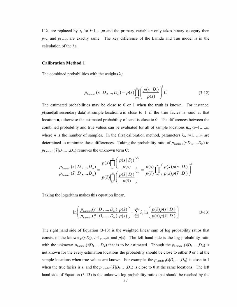
37

If λi are replaced by τi for i=1,…,m and the primary variable s only takes binary category then

pTau and pLamda are exactly same. The key difference of the Lamda and Tau model is in the

calculation of the λs.

Calibration Method 1

The combined probabilities with the weights λi:

1 11

( | )( | ,..., ) ( )( )

imi

Lamda mi

p s Dp s D D p s Cp s

λ

=

⎛ ⎞= ⎜ ⎟

⎝ ⎠∏ (3-12)

The estimated probabilities may be close to 0 or 1 when the truth is known. For instance,

p(sand|all secondary data) at sample location u is close to 1 if the true facies is sand at that

location u, otherwise the estimated probability of sand is close to 0. The differences between the

combined probability and true values can be evaluated for all of sample locations uα, α=1,…,n,

where n is the number of samples. In the first calibration method, parameters λi, i=1,…,m are

determined to minimize these differences. Taking the probability ratio of pLamda 1(s|D1,…,Dm) to

pLamda 1( s |D1,…,Dm) removes the unknown term C:

11 1

11 1

1

( | )( )( )( | ,..., ) ( ) ( | )( )

( | ,..., ) ( ) ( ) ( | )( | )( )( )

i

i

i

mi

miLamda m i

m iLamda m ii

i

p s Dp sp sp s D D p s p s Dp s

p s D D p s p s p s Dp s Dp sp s

λ

λ

λ=

=

=

⎛ ⎞⎜ ⎟ ⎛ ⎞⎝ ⎠= = ⎜ ⎟⎛ ⎞ ⎝ ⎠⎜ ⎟⎝ ⎠

∏∏

∏

Taking the logarithm makes this equation linear,

1 1

11 1

( | ,..., ) ( ) ( | )( )ln ln( | ,..., ) ( ) ( ) ( | )

mLamda m i

iiLamda m i

p s D D p s p s Dp sp s D D p s p s p s D

λ=

⎛ ⎞ ⎛ ⎞=⎜ ⎟ ⎜ ⎟

⎝ ⎠ ⎝ ⎠∑ (3-13)

The right hand side of Equation (3-13) is the weighted linear sum of log probability ratios that

consist of the known p(s|Di), i=1,…,m and p(s). The left hand side is the log probability ratio

with the unknown pLamda1(s|D1,…,Dm) that is to be estimated. Though the pLamda 1(s|D1,…,Dm) is

not known for the every estimation locations the probability should be close to either 0 or 1 at the

sample locations when true values are known. For example, the pLamda 1(s|D1,…,Dm) is close to 1

when the true facies is s, and the pLamda1( s |D1,…,Dm) is close to 0 at the same locations. The left

hand side of Equation (3-13) is the unknown log probability ratios that should be reached by the

38

weighted linear combination of log ratios of conditional probabilities and global proportions in

the right hand side. Since we have many pairs of input probabilities corresponding to the number

of samples (n), Equation (3-13) can be expressed as a matrix equation:

1 1 1 1 2 1 1

2 2 1 2 2 2 2

1 2

( ; ) ( ; | ) ( ; | ) ( ; | )( ; ) ( ; | ) ( ; | ) ( ; | )

( ; ) ( ; | ) ( ; | ) ( ; | )or

m

m

n n n n m m

b s a s D a s D a s Db s a s D a s D a s D

b s a s D a s D a s D

λλ

λ

⋅⋅⋅⎡ ⎤ ⎡ ⎤ ⎡ ⎤⎢ ⎥ ⎢ ⎥ ⎢ ⎥⋅⋅⋅⎢ ⎥ ⎢ ⎥ ⎢ ⎥=⎢ ⎥ ⎢ ⎥ ⎢ ⎥⋅⋅⋅⎢ ⎥ ⎢ ⎥ ⎢ ⎥⋅⋅⋅⎣ ⎦ ⎣ ⎦ ⎣ ⎦

= •

u u u uu u u u

u u u u

B A λ (3-14)

a(u1;s|D1), for example, represents 1

1

( | ) ( )ln ( | ) ( )p s D p s

p s D p s⎛ ⎞⎜ ⎟⎝ ⎠

at the location u1 where

the truth is s, b(u1;s) represents a target value at the location u1

1 1

1 1

( | ,..., ) ( )ln .( | ,..., ) ( )Lamda m

Lamda m

p s D D p sp s D D p s

⎛ ⎞⎜ ⎟⎝ ⎠

Note that the complementary

probability in the denominator of a(uα;s|Di) and b(uα;s) cannot be zero. In practice, a very small

value would be substituted for the exact zero probability in the denominator of b(uα;s), α=1,…,n.

The unknown weights are derived by minimizing the squared differences between B and Aλ such

as ||B - Aλ||2. The least square n solution of λ can be followed as:

1( ' ) '−=λ A A A B (3-15)

where A′ is the transpose of A. Figure 3.1 illustrates graphically how to build elements of the

matrix Equation (3-14). Two secondary data D1 and D2 are assumed to be processed to make

p(s|D1) and p(s|D2) where s takes ternary codes represented as black, dark and light gray colors.

Based on 7 well samples where the true facies are known, matrices for calculating weights are

built. The weights λi are obtained by accounting for the closeness of the combined probabilities

to the true probabilities at sample locations.

The motivation for putting weight parameters is to mitigate the independence assumption

made in the simple combination model. The levels of redundancy between the secondary data

may be different depending on different s. When taking the probability ratios in Equation (3-13),

however, λs are assumed to be independent of s.

39

Figure 3.1: A graphical illustration for calculating weights using weight calibration method 1. Weights are calculated based on the differences between true and combined probabilities.

1 1 1 1 2

2 2 1 2 2

3 3 1 3 2

4 4 1 4 2

5 5 1 5 2

6 6 1

7

( ; ) ( ; , ) ( ; , )( ; ) ( ; , ) ( ; , )( ; ) ( ; , ) ( ; , )( ; ) ( ; , ) ( ; , )( ; ) ( ; , ) ( ; , )( ; ) ( ; , )( ; )

b E a E D a E Db E a E D a E Db E a E D a E Db E a E D a E Db E a E D a E Db E a E Db E

= = =⎡ ⎤⎢ ⎥= = =⎢ ⎥⎢ ⎥= = =⎢ ⎥= = = =⎢ ⎥⎢ ⎥= = =⎢ ⎥

= =⎢ ⎥⎢ ⎥=⎣ ⎦

u u uu u uu u uu u uu u uu uu

1

2

6 2

7 1 7 2

( ; , )( ; , ) ( ; , )

a E Da E D a E D

λλ

⎡ ⎤⎢ ⎥⎢ ⎥⎢ ⎥

⎡ ⎤⎢ ⎥⎢ ⎥⎢ ⎥⎣ ⎦⎢ ⎥

⎢ ⎥=⎢ ⎥

⎢ ⎥= =⎣ ⎦

uu u

p(s= |D2)

p(s= |D2)

p(s= |D2)

p(s= |D1)

p(s= |D1)

p(s= |D1)

u1u3

u4u5 u6

u7

u2

1 2

1 21 2

( | ) ( | )( | , ) ( )( ) ( )Lamda

p E D p E Dp E D D p E Cp E p E

λ λ⎛ ⎞ ⎛ ⎞= =

= = = ⎜ ⎟ ⎜ ⎟= =⎝ ⎠ ⎝ ⎠

Matrix for weights calculation

well data

1 2

1 21 2

( | ) ( | )( | , ) ( )( ) ( )Lamda

p E D p E Dp E D D p E Cp E p E

λ λ⎛ ⎞ ⎛ ⎞= =

= = = ⎜ ⎟ ⎜ ⎟= =⎝ ⎠ ⎝ ⎠

1 2

1 21 2

( | ) ( | )( | , ) ( )( ) ( )Lamda

p E D p E Dp E D D p E Cp E p E

λ λ⎛ ⎞ ⎛ ⎞= =

= = = ⎜ ⎟ ⎜ ⎟= =⎝ ⎠ ⎝ ⎠

sssssss

sssssss

sssssss

s

s

s

s s s

ss

ss

ss

ss

s s

s

s

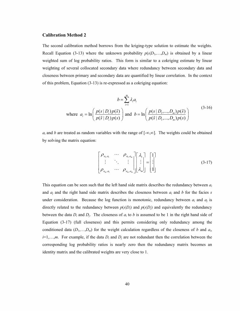
40

Calibration Method 2

The second calibration method borrows from the kriging-type solution to estimate the weights.

Recall Equation (3-13) where the unknown probability p(s|D1,…,Dm) is obtained by a linear

weighted sum of log probability ratios. This form is similar to a cokriging estimate by linear

weighting of several collocated secondary data where redundancy between secondary data and

closeness between primary and secondary data are quantified by linear correlation. In the context

of this problem, Equation (3-13) is re-expressed as a cokriging equation:

1

1

1

( | ) ( ) ( | ,..., ) ( )where ln and ln( | ) ( ) ( | ,..., ) ( )

m

i ii

i mi

i m

b a

p s D p s p s D D p sa bp s D p s p s D D p s

λ=

=

⎛ ⎞ ⎛ ⎞= =⎜ ⎟ ⎜ ⎟

⎝ ⎠ ⎝ ⎠

∑ (3-16)

ai and b are treated as random variables with the range of [-∞,∞]. The weights could be obtained

by solving the matrix equation:

1 1 1

1

, , 1

, ,

1

1

m

m m m

a a a a

a a a a m

ρ ρ λ

ρ ρ λ

⎡ ⎤ ⎡ ⎤ ⎡ ⎤⎢ ⎥ ⎢ ⎥ ⎢ ⎥=⎢ ⎥ ⎢ ⎥ ⎢ ⎥⎢ ⎥ ⎢ ⎥ ⎢ ⎥⎣ ⎦ ⎣ ⎦⎣ ⎦

(3-17)

This equation can be seen such that the left hand side matrix describes the redundancy between ai

and aj and the right hand side matrix describes the closeness between ai and b for the facies s

under consideration. Because the log function is monotonic, redundancy between ai and aj is

directly related to the redundancy between p(s|Di) and p(s|Dj) and equivalently the redundancy

between the data Di and Dj. The closeness of ai to b is assumed to be 1 in the right hand side of

Equation (3-17) (full closeness) and this permits considering only redundancy among the

conditioned data (D1,…,Dm) for the weight calculation regardless of the closeness of b and ai,

i=1,…,m. For example, if the data Di and Dj are not redundant then the correlation between the

corresponding log probability ratios is nearly zero then the redundancy matrix becomes an

identity matrix and the calibrated weights are very close to 1.

41

3.4 1-D Example

A small 1-D example is presented with the different probability combination methods for

graphical convenience. Figure 3.2 illustrates the sampled facies (rectangles), global proportion

(horizontal line) and calibrated conditional probabilities of facies code 1 (three dashed lines) at

every 1m along the horizontal transect. The generated conditional probabilities are positively

correlated each other with moderate-to-high probabilities of the correct facies in which the given

conditioning data D1, D2 and D3 are deemed to be redundant.

Figure 3.2: 1-D example along the horizontal transect. Modeling for the binary category is considered. Three conditioning secondary data D1,D2 and D3 are assumed to redundant since the probabilities p(s|Di) are positively correlated. The global proportion p(s) and the primary hard data ( ) are shown.

p(s|Di) for i=1,2,3 reasonably honors the primary hard data; they correctly inform the presence or

absence of the true facies overall. Inaccuracy of p(s|Di) is intentionally injected into around the

location index of 30 to underline the impact of different combination schemes. As shown in later

in Figure 3.6, the combined probability by the calibration method 1 corrects this artificially

injected inaccuracy. The conditional probability lines are combined using the conditional

independence model first and it is shown in Figure 3.3. Though the conditional independence is

equivalent to the PR model for this particular example (binary category modeling), the

conditional independence approach is only considered as a simple combination method because

the validity of the PR method is not general in multiple facies. The combined probability changes

drastically and it is not within the global and three conditional probability lines except in

transition zones where the conditional probabilities pass by the global proportion. The

combination method that makes the combined probability close to 0 or 1 seems to reduce the

10 20 30 40 500

0.2

0.4

0.6

0.8

1

Locations

Pro

babi

lity

p(s|D1)

p(s)

p(s|D2)p(s|D3)

sample

42

uncertainty in the final combined probability, and shows a high closeness to the true values at

sample locations. In particular, when the elementary conditional probabilities are highly

redundant, the combined probability should not be far away from the input conditional probability.

The danger of the conditional independence model is overfitting that would harm the fairness of

the final probability.

Figure 3.3: The combined probability using the conditional independence model (pCI).

The result of the Lamda model with the first calibration method is shown in Figure 3.4. The

calibration method computes the weights by minimizing the differences between the combined

probability and the true probability at sample locations. For the present 1-D example, 28 samples

are used to build the matrix equation 3-15: the individual conditional probabilities at 28 sample

locations constitute the matrix A, the true probability at sample locations constitute the vector B.

Care must be taken in building the vector B because the log ratio in the vector B becomes infinity

when the complementary probability p( s |D1,…,Dm) in the denominator has zero probability

when the true facies is s. To overcome this numerical instability, a minimum bound of

probability (denoted as ε) is used instead of exactly zero in the elements of the vector B. The

combined probability shown at the top of Figure 3.4 is obtained by substituting ε=0.001 for zero

and it overfits more than the conditional independence model. This is due to the fact that the

considered weight calibration method calculates the weight not by accounting for the redundancy

but by minimizing the least square errors. Thus, the wi parameters are chosen to make the

resulting probability as close as possible to the true probability (either 0 or 1) at sample locations.

Note, however, that the overfitting can be controlled by adjusting the artificial small value of

probability that is used when building the vector B in Equation (3-15). As smaller value is used,

the differences between the true and combined probability are elevated more, and thus the

10 20 30 40 500

0.2

0.4

0.6

0.8

1

Locations

Pro

babi

lity

pCI

43

magnitude of the weights becomes larger to minimize these differences. The bottom of Figure

3.4 shows several combined probability lines using the different ε. The use of small ε (such as

0.001) leads to overfit combined probabilities. The use of a relatively large value such as ε=0.1,

on the contrary, mitigates the accuracy of the elementary probabilities p(s|Di). The combined

probability should be reasonably close to the true probability where we know the correct facies

and it should be fair as well. Cross validation such as accuracy assessment discussed in Section

3.6 could be used for selecting the appropriate small value of ε.

Figure 3.4: The combined probability using the Lamda model with the first calibration method. To avoid the numerical instability, an artificial small value (ε) is injected to the calibration equation and the results become different based on the used small values.

Unlike the first calibration method, the second calibration method accounts for the redundancy

among the individual conditional probability obtained from each data. Equation (3-17) for

obtaining the weight is established as below,

10 20 30 40 500

0.2

0.4

0.6

0.8

1

Locations

Pro

babi

lity

10 20 30 40 500

0.2

0.4

0.6

0.8

1

Locations

Pro

babi

lity

pLamda1 with ε=0.001

pLamda1 with ε=0.001

pLamda1 with ε=0.03

pLamda1 with ε=0.1

44

1

2

3

1 0.903 0.94 10.903 1 0.89 10.94 0.89 1 1

λλλ

⎡ ⎤ ⎡ ⎤ ⎡ ⎤⎢ ⎥ ⎢ ⎥ ⎢ ⎥=⎢ ⎥ ⎢ ⎥ ⎢ ⎥⎢ ⎥ ⎢ ⎥ ⎢ ⎥⎣ ⎦ ⎣ ⎦ ⎣ ⎦

The weights are derived by solving the matrix equation:

Weights from calibration method 2

λ1 0.253

λ2 0.448

λ3 0.364

The calibrated weights are smaller than 1 because of the high correlation between the input

conditional probabilities. If the data had little redundancy (small correlation in the left hand side

matrix) then the weights would be close to 1. The data D1 receives the smallest weight and the

weight λ1=0.253 reduces the influence of p(s|D1)/p(s). The data D2 receives the largest weight

and the weight λ2=0.448 least reduces the influence of p(s|D2)/p(s). The combined probability

with the obtained weights above is shown in Figure 3.5. Weights less than 1 weaken the effect of

the non-convexity such as reducing the contribution of the probability ratio p(s|Di)/p(s) to the

final probability. For example, if the probability ratio is less than 1 then the weighted probability

ratio is increased by the applied weight less than 1, and thus the combined probability becomes

not far below the input p(s|Di) and p(s). Likewise, if the probability ratio is greater than 1 then

the weighted probability ratio is decreased by applying the weight less than 1, and the combined

probability becomes not far above the input p(s|Di) and p(s). In particular, if the given data are

highly redundant such as in this example, the calibration method 2 generates small weights that

make the probabilities more reasonable and less overfit.

One interesting aspect about the calculated weights from the second calibration method is

that their sum could represent the overall data redundancy quantitatively. For example, the sum

of the calculated weights for the illustrated 1-D example is about 1.06 and intuitively, this could

be interpreted that three conditioning data D1, D2 and D3 are regarded virtually as a single data.

The sum of weights would be interpreted as following:

45

Interpretations

1

m

ii

mλ=

≈∑ m secondary data are nearly independent

1

m

ii

mλ=

<∑ m secondary data are somewhat redundant

The overall redundancy among the given secondary data could be quantified as

( )11 /m

iimλ

=⎡ ⎤−⎢ ⎥⎣ ⎦∑ × 100 in %.

Figure 3.5: The combined probability using the Lamda model with the second calibration method.

The combined probabilities with the different combination schemes are demonstrated together in

one plot in Figure 3.6. The uncertainty in the final probability is decreased after integrating

different probabilities conditioned to the diverse data; however, the degree of reduction in the

uncertainty is different for each combination scheme. The simple combination method assumes

that the given conditioning data are independent and the method makes the probability quite

extreme. As mentioned previously, this overfitting becomes more risky when the given

secondary data redundant. The weighted combination methods do not pull the resulting

probability toward extremes as much as the simple combination method does. Among the two

calibration methods for the Lamda model, the result with the least square calibration method

honors the true values at sample locations very well and especially the result is in a good

accordance with the samples around 30m where other methods cannot account for. This is due to

the fact that the conditional independence and the Lamda model with the second calibration

10 20 30 40 500

0.2

0.4

0.6

0.8

1

Locations

Pro

babi

lity

pLamda 2

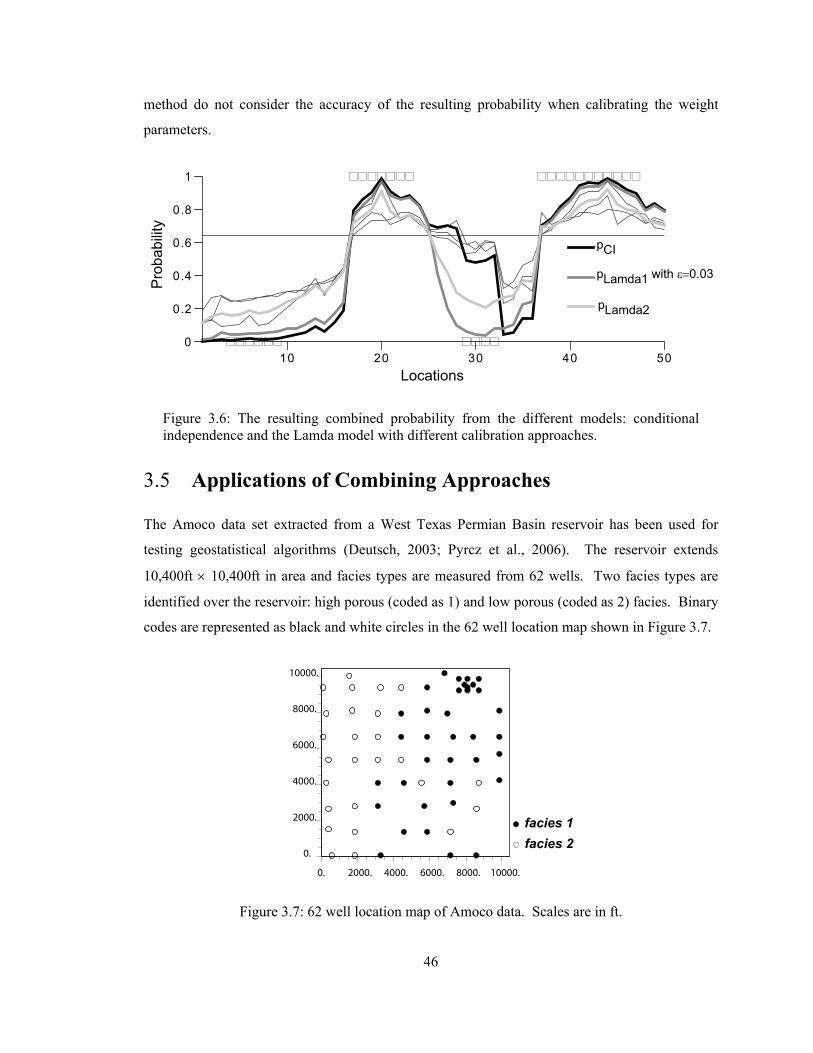
46

method do not consider the accuracy of the resulting probability when calibrating the weight

parameters.

Figure 3.6: The resulting combined probability from the different models: conditional independence and the Lamda model with different calibration approaches.

3.5 Applications of Combining Approaches

The Amoco data set extracted from a West Texas Permian Basin reservoir has been used for

testing geostatistical algorithms (Deutsch, 2003; Pyrcz et al., 2006). The reservoir extends

10,400ft × 10,400ft in area and facies types are measured from 62 wells. Two facies types are

identified over the reservoir: high porous (coded as 1) and low porous (coded as 2) facies. Binary

codes are represented as black and white circles in the 62 well location map shown in Figure 3.7.

Figure 3.7: 62 well location map of Amoco data. Scales are in ft.

10 20 30 40 500

0.2

0.4

0.6

0.8

1

Locations

Pro

babi

lity

pCI

pLamda1 with ε=0.03

pLamda2

facies 1facies 2

0. 2000. 4000. 6000. 8000. 10000.

0.

2000.

4000.

6000.

8000.

10000.

47

A seismic amplitude data is available over the area. The seismic measurements at the 62 well

locations are calibrated with the facies type at those locations. Nonparametric statistical

distribution modeling was used to build the probability distributions. Figure 3.8 illustrates the

seismic data map (left) and the calibrated facies probability distributions (middle). Well data

shown in the seismic amplitude map are used for the probability distribution calibration. Based

on the modeled probability distributions, the conditional probability of facies given the seismic

value is extracted. A 2-D map shown in the right of Figure 3.8 represents the probability of facies

1 given the seismic data.

Figure 3.8: A seismic amplitude map (left), probability distributions calibrated from the 62 wells (centre), and the derived facies probability map (right).

There is one secondary data available. Two more secondary data are generated to illustrate the

effect of integrating several secondary data. A trend is considered as secondary information and

it is generated using the 62 well data. Trends are important features that should be adequately

accounted for in the final geostatistical model. Simple indicator kriging with an isotropic

variogram using a large range (half of the domain) is used to make a smooth map of facies trend.

Explicit modeling of the trend and incorporating the trend into the final geostatistical model is a

widely used approach. Figure 3.9 shows the modeled trend of facies 1.

42000

56000

0.0

1.0

40000 44000 48000 52000 56000

Seismic amplitude

Seismic amplitude

Pro

babi

lity

Probability of facies 1

p(s=1|seis)p(s=2|seis)

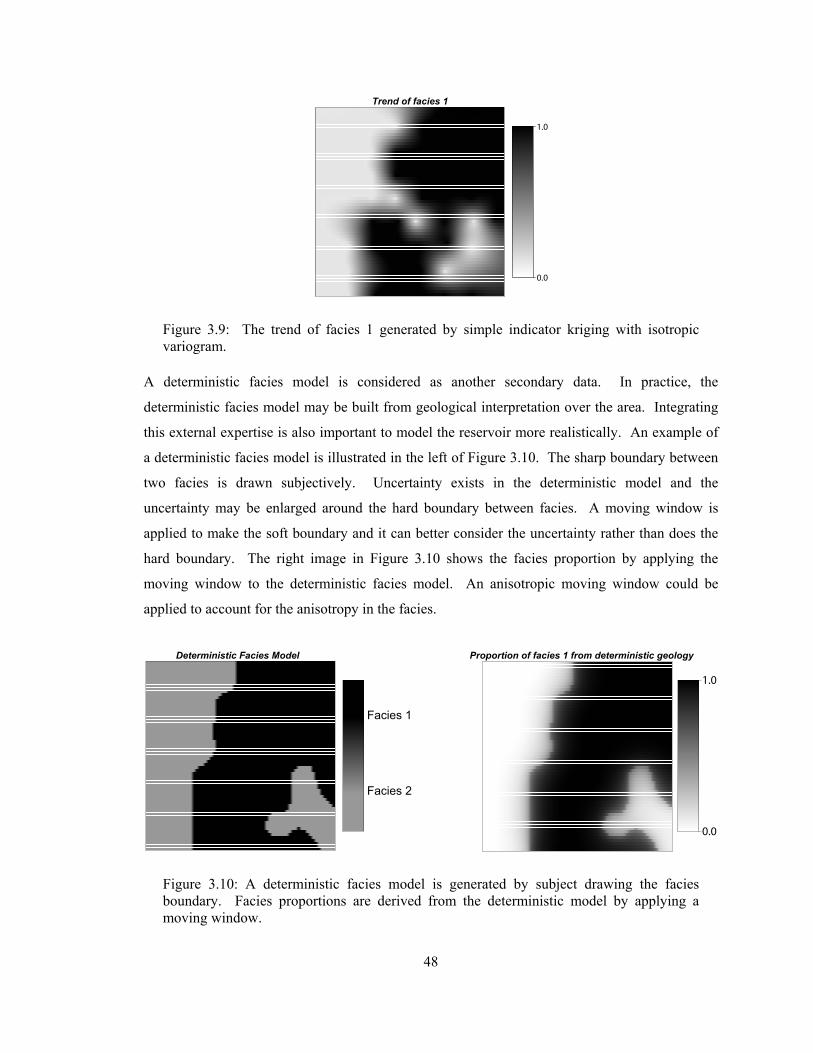
48

Figure 3.9: The trend of facies 1 generated by simple indicator kriging with isotropic variogram.

A deterministic facies model is considered as another secondary data. In practice, the

deterministic facies model may be built from geological interpretation over the area. Integrating

this external expertise is also important to model the reservoir more realistically. An example of

a deterministic facies model is illustrated in the left of Figure 3.10. The sharp boundary between

two facies is drawn subjectively. Uncertainty exists in the deterministic model and the

uncertainty may be enlarged around the hard boundary between facies. A moving window is

applied to make the soft boundary and it can better consider the uncertainty rather than does the

hard boundary. The right image in Figure 3.10 shows the facies proportion by applying the

moving window to the deterministic facies model. An anisotropic moving window could be

applied to account for the anisotropy in the facies.

Figure 3.10: A deterministic facies model is generated by subject drawing the facies boundary. Facies proportions are derived from the deterministic model by applying a moving window.

Trend of facies 1

0.0

1.0

Deterministic Facies Model

Facies 2

Facies 1

Proportion of facies 1 from deterministic geology

0.0

1.0

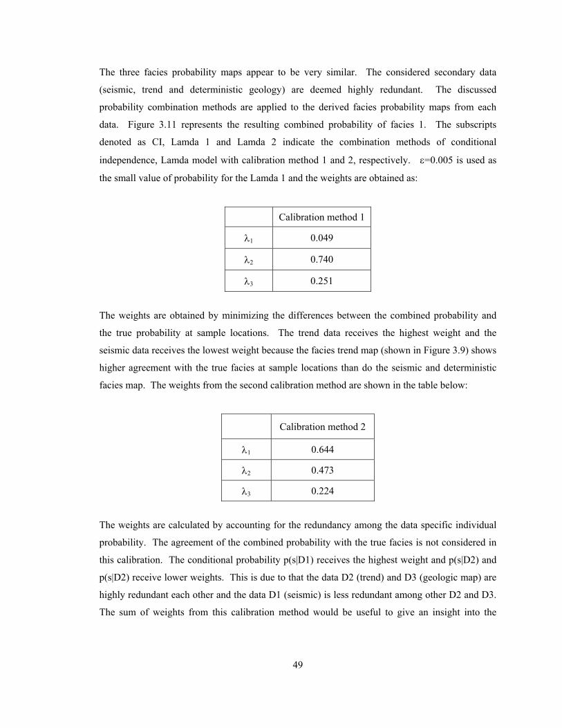
49

The three facies probability maps appear to be very similar. The considered secondary data

(seismic, trend and deterministic geology) are deemed highly redundant. The discussed

probability combination methods are applied to the derived facies probability maps from each

data. Figure 3.11 represents the resulting combined probability of facies 1. The subscripts

denoted as CI, Lamda 1 and Lamda 2 indicate the combination methods of conditional

independence, Lamda model with calibration method 1 and 2, respectively. ε=0.005 is used as

the small value of probability for the Lamda 1 and the weights are obtained as:

Calibration method 1

λ1 0.049

λ2 0.740

λ3 0.251

The weights are obtained by minimizing the differences between the combined probability and

the true probability at sample locations. The trend data receives the highest weight and the

seismic data receives the lowest weight because the facies trend map (shown in Figure 3.9) shows

higher agreement with the true facies at sample locations than do the seismic and deterministic

facies map. The weights from the second calibration method are shown in the table below:

Calibration method 2

λ1 0.644

λ2 0.473

λ3 0.224

The weights are calculated by accounting for the redundancy among the data specific individual

probability. The agreement of the combined probability with the true facies is not considered in

this calibration. The conditional probability p(s|D1) receives the highest weight and p(s|D2) and

p(s|D2) receive lower weights. This is due to that the data D2 (trend) and D3 (geologic map) are

highly redundant each other and the data D1 (seismic) is less redundant among other D2 and D3.

The sum of weights from this calibration method would be useful to give an insight into the

50

overall redundancy; 55% (1– 3

1/ 3ii

λ=∑ =1–0.45) information from the each data is redundant on

the average.

51

Figure 3.11: The estimated facies probabilities from three different combination schemes: the conditional independence (top), Lamda model with calibration method 1 (middle) and 2 (bottom).

Conditional Independence

Lamda Model with Calibration Method 1

Lamda Model with Calibration Method 2

0.0

1.0

0.0

1.0

0.0

1.0

52

Non-convex Property of the Combined Probability

The non-convex property refers to the situation when the integrated probability is not within the

range of the input probabilities p(s|Di) and the global proportion p(s). Non-convexity is natural in

data integration. Integrating diverse data amplifies the impact of data sources if they represent

the same direction of probability. The degree of non-convexity is affected by how redundant the

data Di are among themselves. Although all of the elementary probabilities p(s|Di) are in the

same direction (they are all higher or lower than the global p(s)), non-convexity may not be

significant when data are highly redundant, and thus the combined probability should not be very

high or very low for this case. Plotting the input individual probabilities and the integrated

probability is useful to check the degree of non-convexity of the result and checking the non-

convexity would be a justification for the calculated goodness measure that will be mentioned in

the next section. Figure 3.12 shows the scatter plots between the input individual probabilities

and the combined probability from the considered different combination methods. Plotting is

performed only when the input probabilities are greater than the global proportion for the facies 1

(p(s=1)=0.514). The individual probabilities greater than the global proportion are along the

abscissa and the combined probability with these individual probabilities are along the ordinate.

Points falling above the diagonal line represents non-convexity. The conditional independence

model shows stronger non-convexity than the weighted combination schemes. The independence

approach always leads to a combined probability that is higher than any of the input individual

probabilities. In other words, the compounding effect of corroborating information is the most

significant in the conditional independence model. In the plots from the weighted combination,

the majority of points are plotted above the diagonal line. The departure from the line and the

non-convexity are not so dramatic as the independence approach. Some points are plotted below

the diagonal line, which indicates the integrated probability becomes even smaller than the input

individual probabilities; 7% and 22% of total plotted dots are below the diagonal line for the

Lamda model with the weight calibration method 1 and 2, respectively. This is because the

weights are not calculated locally but globally.

53

Figure 3.12: Cross plots for showing the non-convex behavior of the combined probability; the input individual probabilities p(s=1|Di) for i=1,2,3 and the combined probabilities p(s=1|D1,D2,D3) from the different combination methods are plotted. Plotting is made when the p(s|Di) for i=1,2,3 are all greater than the global proportion p(s=1)=0.514.

54

The non-convexity is observed in Figure 3.12 when the input probabilities are larger than the

global proportion, however, the same result can be made for the case of plotting probabilities

smaller than the global proportion.

Although the non-convexity is a desirable property in data integration in terms of making the

final integrated probability be a certainty (push toward 0 or 1), the magnitude of non-convexity

relies on how redundant the data are, and thus the reasonableness must be judged by

understanding and quantifying the data redundancy. Alternatively, the resulting integrated

probability is directly assessed by cross validation techniques so as to check the reasonableness of

the applied weights and the non-convex behavior.

3.6 Accuracy Assessment

If the additional information is properly combined, integrating the secondary data helps build a

reservoir model with less uncertainty and high accuracy. The relevance between the secondary

and the primary data must be fully utilized and redundancy between secondary data is reasonably

accounted for. Secondary derived facies probabilities are evaluated before being incorporated in

sequential simulation for building the final facies model. There is a classical measure of

performance that assigns the most likely facies with a maximum probability and then count the

actual and predicted pixel number. A confusion matrix summarizes these results (Johnson and

Wichern, 2002):

Predicted pixel number

Actual pixel number

Facies 1 Facies 2

Facies 1 n11 n12

Facies 2 n21 n22

For example, n11 is the number of pixels correctly classified as facies 1 and n21 is the number of

pixels actually facies 1 that are misclassified. The classification accuracy of facies 1 is then

calculated by n11/(n11+n12). This simple evaluation method does not consider the uncertainty or

probabilities. Figure 3.13 illustrates a drawback of accuracy calculation using the classical

confusion matrix. A small 4 grid example is shown for illustration.

55

Figure 3.13: Small example showing the risk of the classical accuracy measure.

Probabilities around 0.5 are assigned at each location which introduces high uncertainty when

assigning facies 1 or 2 with the largest probability. Classification accuracy is calculated as 0%

for both facies. Based on 0% classification accuracy, it might be concluded that the secondary

data is useless when one wants to use them for identifying facies or the considered probabilistic

model is completely invalid. The classical accuracy measure does not account for the high degree

of uncertainty indicated by the estimated probability just below and above 0.5.

Reproduction of Global Proportions

Close reproduction of the global proportions is a quick check. The average of p(s|D1,D2,D3) over

the domain should be close to the representative global proportions of s. The reproduced

proportions from the different combination methods for the previous example are summarized.

Facies 1 (s=1) Facies 2 (s=2)

1 2 3( | , , )CIp s D D D 0.597(16.1%) 0.403(17.1%)

1 1 2 3( | , , )Lamdap s D D D 0.57(10.8%) 0.43(11.3%)

2 1 2 3( | , , )Lamdap s D D D 0.575(11.9%) 0.425(12.6%)

Differences in % with the input global proportions are shown in the parentheses. The

combination models reasonably reproduce the input proportions.

pS(s=1)

pS(s=2)

true facies

true facies

facies classification

Accuracy=0 %

Accuracy shown asclosenessCs=1 = 0.46Cs=2 = 0.48

assign withmax. prob

k=1 k=2

0.46 0.51

0.52 0.53

compare totrue facies

calculate Cs0.46 0.51

0.52 0.53

56

Accuracy of Local Estimated Probabilities

The next criterion is to assess the accuracy or fairness of the locally estimated probabilities.

When a model predicts the occurrence of sand with 10% probability, there should be actually be

sand at about 10% of those locations (Isaaks and Srivastava, 1989; Deutsch, 1997). The locally

estimated probabilities can be said to be accurate or fair if they reflect the true fraction of times

the predicted facies occurs (Deutsch, 2002). For example, consider all locations where we predict

0.3 probability of sand, then it is fair that 30% of those locations are sand. A fairness check is

conducted over 0 – 100% prediction intervals with user-input incremental levels. The fairness

measure is:

{ }Actual Fraction ( ; ) | ( ; ) , , 1,...,E I s p s p p s Kα α= = ∀ =u u (3-18)

where p(uα;s) are probabilities at sample location uα, α=1,…,n. p is a predicted probability.

Indicator function I(⋅) takes either 0 or 1 depending on facies type s. The actual fraction at p is an

average of indicator values under the predicted p. This actual fraction is calculated at all p values

and then plotted against p. The predicted probability and the actual fractions could be

summarized in a table:

Table 3.1: An example of the fairness measure for categorical variable

Predicted probability p

Total number (n0) of samples predicted as p

Actual number (n1) of samples identified as

facies s among n0

Actual fractions (n1/n0)

Ideal fractions

0.05 – 0.15 3 20 0.15 0.1

• • •

• • •

• • •

• • •

• • •

0.95 – 1.15 9 10 0.9 1.0

Sum Total sample number (n)

Total sample number of facies s (ns)

- -

The most fair or accurate case is when the actual fractions are identical to the predicted

probabilities for all intervals of predicted p. The calculated actual fractions, however, are

affected by the number of samples. For instance, if the total number of samples is 30 and

predicted probabilities have intervals of 0.1 then each interval of predicted probabilities might

57

have very few number of samples at the given predicted p, that is, 3 on the average. The

calculated fractions may be close to 0 in a low predicted p and close to 1 in a high predicted p.

Figure 3.14 shows the fairness measure in one plot. The plots shown in Figure 3.14 are overall

fairness measure (all facies), but one can plot by-facies fairness plot. Distant plotting from the

diagonal line will be a problem; falling in the lower area would suggest an overfitting of the

estimated probability to the sample data and falling in the above area would indicate the

probability of the facies but not to the extent of a high enough probability. Probability intervals

of 0.1 are applied to the predicted probability. The corresponding actual fractions are plotted as

dots. Plotting is not made when the actual fractions with zero number of n0 in which the actual

fractions cannot be computed. This qualitative checking method is aimed at identifying the case

where the actual fractions are significantly departed from the given predicted probability

(Deutsch, 1999). Figure 3.14 shows that the results from different combination schemes

accurately reflect the true fraction of times predicted facies present only when very high or very

low predicted probabilities are given. For this particular example, this may be caused by that the

elementary probabilities p(s|Di) are very extreme so that the combined probabilities are toward

extreme as well. The result from the independence model is relatively inaccurate given the

intermediate predicted probabilities of 0.45-0.55.

Figure 3.14: Fairness plots of the combined probabilities from different combination models. The plotted fairness measure is averaged over facies s=1,2.

3.7 Building High Resolution Stochastic Model

If the secondary data have been integrated to the units of the primary attribute, indicator kriging

can be used to integrate that information into an improved conditional probability for sequential

simulation. The uncertainty from different methods for integrating diverse secondary data will be

used in simulated realizations. Poor results caused by invalid secondary data integration methods

Act

ual F

ract

ions

Fairness plot of pCI Fairness plot of pLamda1 Fairness plot of pLamda2

0.00 0.20 0.40 0.60 0.80 1.000.00

0.20

0.40

0.60

0.80

1.00

Act

ual F

ract

ions

0.00 0.20 0.40 0.60 0.80 1.000.00

0.20

0.40

0.60

0.80

1.00

Act

ual F

ract

ions

0.00 0.20 0.40 0.60 0.80 1.000.00

0.20

0.40

0.60

0.80

1.00

Predicted probability Predicted probability Predicted probability

58

could lead to worse results and could be amplified during the simulation. This section describes

how the simulated facies realizations are affected by the different probability combination

methods. No direct comparison with the reference reservoir responses will be performed. Instead,

statistical consistency checks are done in terms of reasonable reproduction of the input statistics.

The Bayesian updating technique is adopted inside the sequential simulation to build the

local probability conditioned to the collocated secondary derived estimate and nearby primary

indicators,

sec

1 2 3( ( ) | ( ), ( ), ( ))*( ; )**( ; ) ( )( ) ( )

p s D D Di si s p s Cp s p s

=u u u uuu (3-19)

where i**(u;s) are the updated local probabilities for simulation, psec(s|D1,D2,D3) is the secondary-

derived probability of facies s. The full derivation of Equation (3-19) is described in section 2.2.4.

The superscript sec indicates different probability combination methods such as the CI, Lamda

model with weight calibration method 1 and 2. C is a normalizing constant to ensure a licit

probability of i**(u;s). Experimental and the fitted variogram are shown in Figure 3.15. As a

large scale feature, the facies has anisotropic spatial variation with N-S as the principal continuity

and E-W as the minor continuity. The small scale features are better modeled with an isotropic

variogram model.

Figure 3.15: Variogram of indicator variable representing facies: experimental variograms (dots) and their fitted variograms (lines).

γ

Distance (ft)

N-S direction

0. 1000. 2000. 3000. 4000. 5000. 6000. 7000.0.00

0.40

0.80

1.20

�

γ

Distance (ft)

E-W direction

0. 1000. 2000. 3000. 4000. 5000. 6000. 7000.0.00

0.40

0.80

1.20

γ(h) = 0.4Sph(h) + 0.6Sph(h)ahmax=2000ahmin=2000

ahmax=30000ahmin=4000

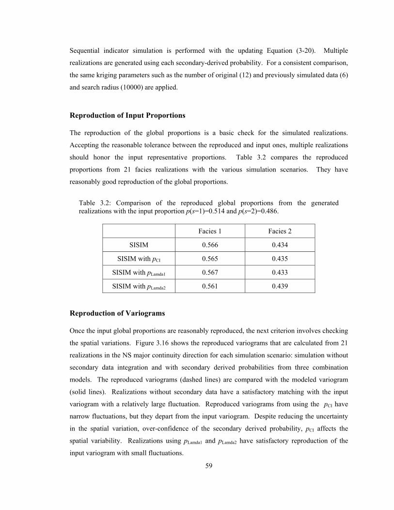
59

Sequential indicator simulation is performed with the updating Equation (3-20). Multiple

realizations are generated using each secondary-derived probability. For a consistent comparison,

the same kriging parameters such as the number of original (12) and previously simulated data (6)

and search radius (10000) are applied.

Reproduction of Input Proportions

The reproduction of the global proportions is a basic check for the simulated realizations.

Accepting the reasonable tolerance between the reproduced and input ones, multiple realizations

should honor the input representative proportions. Table 3.2 compares the reproduced

proportions from 21 facies realizations with the various simulation scenarios. They have

reasonably good reproduction of the global proportions.

Table 3.2: Comparison of the reproduced global proportions from the generated realizations with the input proportion p(s=1)=0.514 and p(s=2)=0.486.

Facies 1 Facies 2

SISIM 0.566 0.434

SISIM with pCI 0.565 0.435

SISIM with pLamda1 0.567 0.433

SISIM with pLamda2 0.561 0.439

Reproduction of Variograms

Once the input global proportions are reasonably reproduced, the next criterion involves checking

the spatial variations. Figure 3.16 shows the reproduced variograms that are calculated from 21

realizations in the NS major continuity direction for each simulation scenario: simulation without

secondary data integration and with secondary derived probabilities from three combination

models. The reproduced variograms (dashed lines) are compared with the modeled variogram

(solid lines). Realizations without secondary data have a satisfactory matching with the input

variogram with a relatively large fluctuation. Reproduced variograms from using the pCI have

narrow fluctuations, but they depart from the input variogram. Despite reducing the uncertainty

in the spatial variation, over-confidence of the secondary derived probability, pCI affects the

spatial variability. Realizations using pLamda1 and pLamda2 have satisfactory reproduction of the

input variogram with small fluctuations.

60

Figure 3.16: Reproduced variograms (dashed lines) from the 21 realizations that are made by different simulation scenarios: simulation with well data only (SISIM) and with integrating secondary derived probabilities obtained from the different methods (SISIM with pCI, pLamda1, pLamda2). The input variogram is shown as heavy sold line.

3.8 Remarks on the PCS

The probability combination schemes are discussed as methods to integrate multiple secondary

data. The approaches indirectly approximate the conditional probability that should be jointly

conditioned to several data through linking the individual probability that are separately

conditioned to each data. A very naïve model assumes the conditional independence between the

given secondary data conditioned to the facies type s. The independence model, however, simply

ignores the redundancy which causes inaccurate resulting combined probability. Weighted

combination models seem to generate reasonable results; however, the calibrated weights are

highly dependent on the calibration procedures. A calibration method 1 with the Lamda model

performs well in particular examples. The combined probability with that calibration method

seems to reasonably account for the redundancy. However, the relation between the calculated

weights and data redundancy is not clearly understood. One way to check the reasonableness of

γ

Distance

SISIM

0. 1000. 2000. 3000. 4000. 5000. 6000.0.00

0.40

0.80

1.20

γ

Distance

SISIM with pCI

0. 1000. 2000. 3000. 4000. 5000. 6000.0.00

0.40

0.80

1.20

γ

Distance0. 1000. 2000. 3000. 4000. 5000. 6000.

0.00

0.40

0.80

1.20

γ

Distance0. 1000. 2000. 3000. 4000. 5000. 6000.

0.00

0.40

0.80

1.20

SISIM with pLamda1 SISIM with pLamda2

61

the calculated weights is to use the pre-defined criteria such as the fairness of the local estimated

probability or reasonable reproduction of the input information from stochastic modeling.

An alternative approach to the PCS is discussed in the next chapter. The new method

directly models the joint distribution among variables and the conditional probability is

immediately derived from the modeled joint distribution. It does not require an external weight

calibration. Instead, the method inherently accounts for the data redundancy during the joint pdf

modeling.

62

Chapter 4

Direct Modeling of

Multivariate Distribution

Chapter 3 investigated probability combination schemes that are calibrated to individual

secondary data. Some theoretical drawbacks and difficulties in quantifying redundancy were

presented.

This chapter investigates directly estimating the joint probability distribution between all

secondary and primary variables instead of approximating the joint probability through linking

the individual probabilities. The proposed idea is motivated by some key points: (1) there are

suitable techniques for modeling the joint relations among variables including nonparametric

approaches and (2) one characteristic of secondary data is exhaustiveness and so the joint

distribution of secondary data can be modeled very reliably. By directly modeling the joint

distribution, data redundancy among variables is accounted for directly. Complicated weight

calibration is no longer required. Moreover, non-Gaussian features between variables can be

captured by applying non-parametric technique. The second motivation related to exhaustiveness

of the secondary data, plays a key role in the proposed approach. The secondary data distribution

is also modeled non-parametrically, but the modeling has very little uncertainty due to the vast

number of samples. One marginality condition of the joint distribution of interest is a reasonable

reproduction of the distribution of secondary variables where the secondary data distribution is

used as a reference marginal distribution. The other marginality condition is the reproduction of

the distribution of the primary variables. The modeled joint distribution between primary and all

63

of secondary variables is evaluated by these conditions and the joint distribution is modified if

differences are observed. An iterative algorithm is developed for the modification.

Section 4.1 discusses the details of kernel density estimation as a nonparametric density

modeling technique. Theoretical analysis on the accuracy of kernel density estimates, choices of

parameters and computational costs are discussed in this section. Section 4.2 investigates the

suggested marginal fitting algorithm that updates the joint distribution in a sequential manner,

termed sequential marginal fitting method. Detailed steps are described for refining the initially

modeled joint distribution under the known reference marginals. The convergence of the

proposed iterative procedure is discussed in Section 4.3.

4.1 Modeling the Multivariate Probability Densities

The joint pdf f(s,D1,…,Dm) is constructed based on the collocated samples of (s,D1,…,Dm)

extracted from wells. One simple way for modeling f(s,D1,…,Dm) is to assume a multivariate

Gaussian distribution between all variables. For example, if porosity is the primary variable of

interest and seismic attributes are the secondary data, then the (m+1) dimensional joint pdf can be

parametrically modeled:

1( 1) / 2 1/ 2 1( ) (2 ) | | exp ( ) ( )

2m tf π −+ − ⎧ ⎫= − − −⎨ ⎬

⎩ ⎭∑ ∑X x x μ x μ (4-1)

where the random vector x consists of porosity and seismic attribute variables. The mean vector

μ and covariance matrix ∑ are calculated at well locations. When the primary variable is not

continuous but categorical variable, the joint distribution would be parametrically modeled based

on categories by (Krzanowski, 1993; Li and Racine, 2003):

1/2 1/2 1( , ) ( )(2 ) | | exp ( ) ( ) , 1,...,

2m t

s sssf s p s s Kπ −− − ⎧ ⎫= − − − =⎨ ⎬⎩ ⎭

∑ ∑y y μ y μ (4-2)

where the joint modeling can be viewed as portioning the f(y) with different outcomes of

categories s=1,…,K. The mean vector μs and covariance matrix Σs are calculated for each

category. The multivariate Gaussian assumption cannot account for non-Gaussian features

between the variables.

Nonparametric density modeling techniques are distribution free methods that do not rely on

the assumption that the data are drawn from a given probability distribution. Various

64

nonparametric density estimation techniques such as the kernel method and its several variants

such as adaptive kernel estimator, maximum likelihood, nearest neighborhood, orthogonal series

estimators have evolved and they have demonstrated satisfactory results in various statistical

discriminant and inference applications (Izenman, 1991; Scott, 1992; Roberts, 1996; Bressan and

Vitria, 2003).

Kernel Density Estimator (Parzen Window Method)

Kernel density estimation (KDE) or the Parzen window method is used for nonparametric

modeling of data distribution since it is widely used and studied (Parzen, 1962; Silverman, 1986).

The KDE method models the data distribution smoothly through applying the kernel function or

weighting function centered on observation data and summing the calculated function values.

The kernel estimate for 1-D is defined by (Parzen, 1962; Silverman, 1986):

1

1( ) for 1 Dn

iKDE

i

x Xf x Wnh h=

−⎛ ⎞= −⎜ ⎟⎝ ⎠

∑ (4-3)

where h is a bandwidth of the applied kernel function, also referred to the smoothing parameter

because h controls the smoothness of the resulting density estimates. W(⋅) is a 1-D kernel

function satisfying W(x)≥0 and ∫W(x)dx = 1 and these conditions make the resulting density

estimates be positive and grand total of densities be 1. Quite often kernel function is taken to be a

standard Gaussian function with mean of 0 and variance of 1. Xi, i=1,…,n is a set of observation

data. Figure 4.1 shows 1-D kernel density estimation example with different bandwidths.

Figure 4.1: Examples of 1-D kernel density estimates with varying bandwidths h. Standard deviation of experimental data σdata is 3.5 and h is arbitrarily chosen with approximately 14%, 28% and 57% of σdata, respectively.

0 4 8 12 16 20 24 0 4 8 12 16 20 24 0 4 8 12 16 20 24

h = 0.5σdata= 3.5 σdata= 3.5 σdata= 3.5

h = 1.0 h = 2.0

65

The shape of the estimated density function changes depending on the choice of kernel bandwidth

h: small h makes less smooth and larger h makes more smooth density estimates. The choice of

bandwidth will be discussed below.

Accuracy of the Estimated Density Functions

Figure 4.1 illustrates the effect of varying the smoothing widths. Improper selection of h could

result in unreliable density estimates: too small h overestimates and too large h underestimates the

sample histogram. Theoretical accuracy analysis of kernel density estimate was investigated by

Rosenblatt (1956) and reviewed by others (Silverman, 1986; Izenman, 1991; Scott, 1992). This

section follows the work of Silverman (1986) to assess the accuracy of kernel density estimate.

The mean integrated square errors (MISE) between fKDE(x) and f(x) are defined as (Silverman,

1986):

{ }2( ( )) ( ) ( )KDE KDEMISE f x E f x f x dx= −∫ (4-4)

Since the integral and expectation operator are commutative, Equation (4-4) gives:

{ }{ }

{ }

2

2

2

( ( )) ( ) ( )

( )

( ) ( ) var ( )

( ) var ( )

KDE KDE

KDE

KDE KDE

KDE

MISE f x E f x f x dx

MSE f x dx

Ef x f x dx f x dx

bias x dx f x dx

= −

=

= − +

= −

∫∫∫ ∫∫ ∫

(4-5)

The mean integrated square error is sum of integrated squared bias and integrated variance.

These terms both depend on h. The bias term is expanded by Taylor expansions (see pages 39–41

in Silverman, 1986) then the integrated squared bias is approximated as:

2 4 22

1( ) w ''( )4

bias x dx h f x dx≈∫ ∫ (4-6)

where w2 is a second derivative term of the kernel function W:

22( ) w 0t W t dt = ≠∫ (4-7)

66

Equation (4-6) shows that bias in the estimation of f(x) is proportional to h: smaller h leads to an

unbiased estimate, and vice versa. Also, the variance term is expanded and shown as:

21var ( ) ( )KDEf x dx W t dtnh

≈∫ ∫ (4-8)

Equation (4-8) shows the variance of fKDE(x) is inversely proportional to h: smaller h makes larger

estimation variance. Comparing Equations (4-6) with (4-8), there is a conflict when choosing an

appropriate h. Attempts to reduce bias increase variance.

Selection of Kernel Bandwidths

The choice of a smoothing parameter is a trade-off in terms of minimizing the mean integrated

square error. Scott (1992) suggested plotting the density estimates and finding the appropriate h

in accordance with the user’s knowledge about the distribution. It should be noted that the

integrated estimation variance, as shown in Equation (4-8), depends not only on h but also on the

number of data n used for density modeling. Increasing the number of samples can relax the

necessity of a large h.

A large volume of literature exists on the selection of optimal bandwidth for kernel density

estimation (Marron 1987; Park and Marron, 1990; Hall et al., 1991; Jones et al., 1996).

Analytical optimal bandwidths were derived to minimize the estimation errors, however, they are

not available in practice since they rely on the true unknown density f. Alternatively, the amount

of smoothness is chosen based on the data. The following equation is an option for selecting the

data driven optimal h (Scott, 1992):

1/ 5ˆ1.06 for 1 Dh nσ −= − (4-9)

where σ̂ is a standard deviation of experimental data. The above relation is derived assuming

that the unknown true density function is a normal distribution with variance 2ˆ .σ Scott (1992)

recommend several attempts with ±20% changes based on the h to finally choose the best

smoothing parameter for the data at hand.

67

Kernel Density Estimation for Multivariate Data

The kernel density estimator in 1-D can be extended in a multivariate case. In its most general

form, the multivariate kernel density estimator is defined by (Silverman, 1986; Wand and Jones,

1996):

( )1

1( ) ( )n

ii

fn =

= −∑ Hx W x X (4-10)

for d-dimension. WH(x)=|H|-1/2W(H-1/2x), W(⋅) is a multivariate kernel function, and H is a

symmetric positive definite d×d matrix known as the bandwidth matrix. The multivariate normal

distribution is usually used as a kernel function W. Similar to the 1-D kernel estimate, the choice

of bandwidth matrix H is crucial to the multivariate density estimates. Sain et al. (1992)

discussed the performance of bootstrap and cross-validation methods for selecting the smoothing

parameters in multivariate density estimation, and found that the complexity of finding an optimal

bandwidth grows prohibitively as the dimension of data increases.

Product Kernel Implementation

Multivariate kernel density estimation requires the multidimensional kernel function WH, which

comes at a cost: inversion of the d×d covariance matrix and matrix multiplications are necessary

for n observation data at each density estimation step. A more practical implementation is to use

product kernel approach which estimates the multivariate densities by multiplying the 1-D kernel

estimates (Cacoullos, 1966; Sain et. al., 1992; Scott, 1992):

1 1, ,

11 1

( ) ( )1( ) W Wn

i d d i

id d

x X x Xf

nh h h h=

− −⎛ ⎞⎛ ⎞= ×⋅⋅⋅× ⎜ ⎟⎜ ⎟×⋅⋅ ⋅× ⎝ ⎠ ⎝ ⎠

∑x (4-11)

for d-dimension. W(⋅) is a 1-D kernel function applied to each variable Xj, j=1,…,d. Kernel

bandwidths hj, j=1,…,d could be different for different variables. Scott (1992) recommended a

data-based optimal bandwidth:

1/( 4)ˆ di ih nσ − += (4-12)

68

The use of the multivariate kernel function described in Equation (4-10) is theoretically correct;

however, the product kernel estimate has little differences in terms of accuracy (Scott, 1992).

Computational Considerations

The flexibility of nonparametric density estimation techniques is placed at the expense of

computational cost. Kernel density estimator used through this work evaluates densities at every

bin where we want to estimate density. For example, if we have 3 variables (1 primary and 2

secondary variables), 30 sample data and we want density estimates at every 50 bins of variables,

then total of 503 × 30 = 3,750,000 calculations are required for constructing a 3-dimensional

probability density functions. The complexity is expressed in general:

(# of variables)(# ) (# of samples)of bins × (4-13)

Practical implementation would limit the number of variables by merging secondary variables.

More than 5 secondary variables should be merged into less than 6 by aggregating closely related

variables

4.2 Marginal Conditions of the Multivariate Distribution

This section is aimed at checking axioms of the joint probability distributions: non negative

density functions, closure condition and reproduction of lower order marginal distributions. The

kernel density estimator meets the first two axioms if the kernel function W(⋅) follows W(x)≥0

and ∫W(x)dx=1. The third condition, reproduction of lower order marginal distribution, is a

marginality condition that the p-variate joint distribution should reproduce p′-variate distribution

where p′ < p. The followings are possible marginal conditions that the modeled joint distribution

f(s,D1,…,Dm) must meet:

1 1( , ,..., ) ( )m mf s D D dD dD p s⋅⋅⋅ ⋅⋅⋅ =∫ ∫ (4-14)

1 11,...,

( , ,..., ) ( ,..., )m ms K

f s D D f D D=

=∑ (4-15)

The marginal relation described in (4-14) states that integration of the multivariate probability

distribution over possible outcomes of the secondary data should amount to the 1-D global

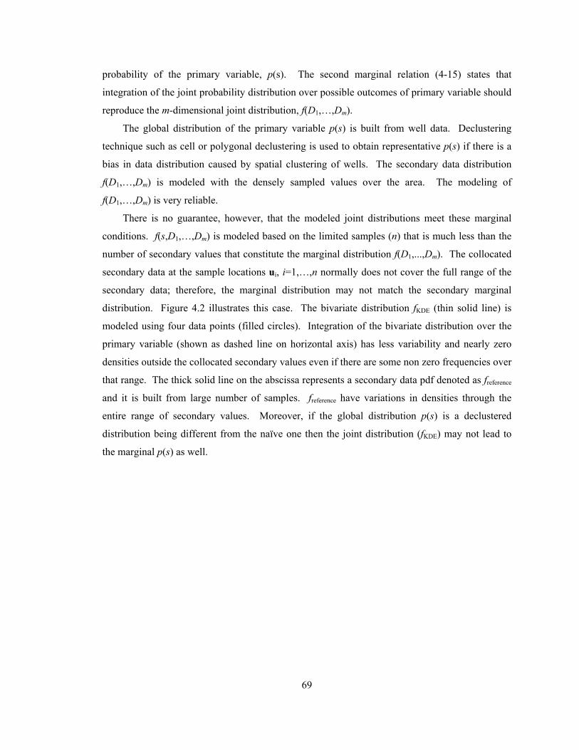
69

probability of the primary variable, p(s). The second marginal relation (4-15) states that

integration of the joint probability distribution over possible outcomes of primary variable should

reproduce the m-dimensional joint distribution, f(D1,…,Dm).

The global distribution of the primary variable p(s) is built from well data. Declustering

technique such as cell or polygonal declustering is used to obtain representative p(s) if there is a

bias in data distribution caused by spatial clustering of wells. The secondary data distribution

f(D1,…,Dm) is modeled with the densely sampled values over the area. The modeling of

f(D1,…,Dm) is very reliable.

There is no guarantee, however, that the modeled joint distributions meet these marginal

conditions. f(s,D1,…,Dm) is modeled based on the limited samples (n) that is much less than the

number of secondary values that constitute the marginal distribution f(D1,...,Dm). The collocated

secondary data at the sample locations ui, i=1,…,n normally does not cover the full range of the

secondary data; therefore, the marginal distribution may not match the secondary marginal

distribution. Figure 4.2 illustrates this case. The bivariate distribution fKDE (thin solid line) is

modeled using four data points (filled circles). Integration of the bivariate distribution over the

primary variable (shown as dashed line on horizontal axis) has less variability and nearly zero

densities outside the collocated secondary values even if there are some non zero frequencies over

that range. The thick solid line on the abscissa represents a secondary data pdf denoted as freference

and it is built from large number of samples. freference have variations in densities through the

entire range of secondary values. Moreover, if the global distribution p(s) is a declustered

distribution being different from the naïve one then the joint distribution (fKDE) may not lead to

the marginal p(s) as well.

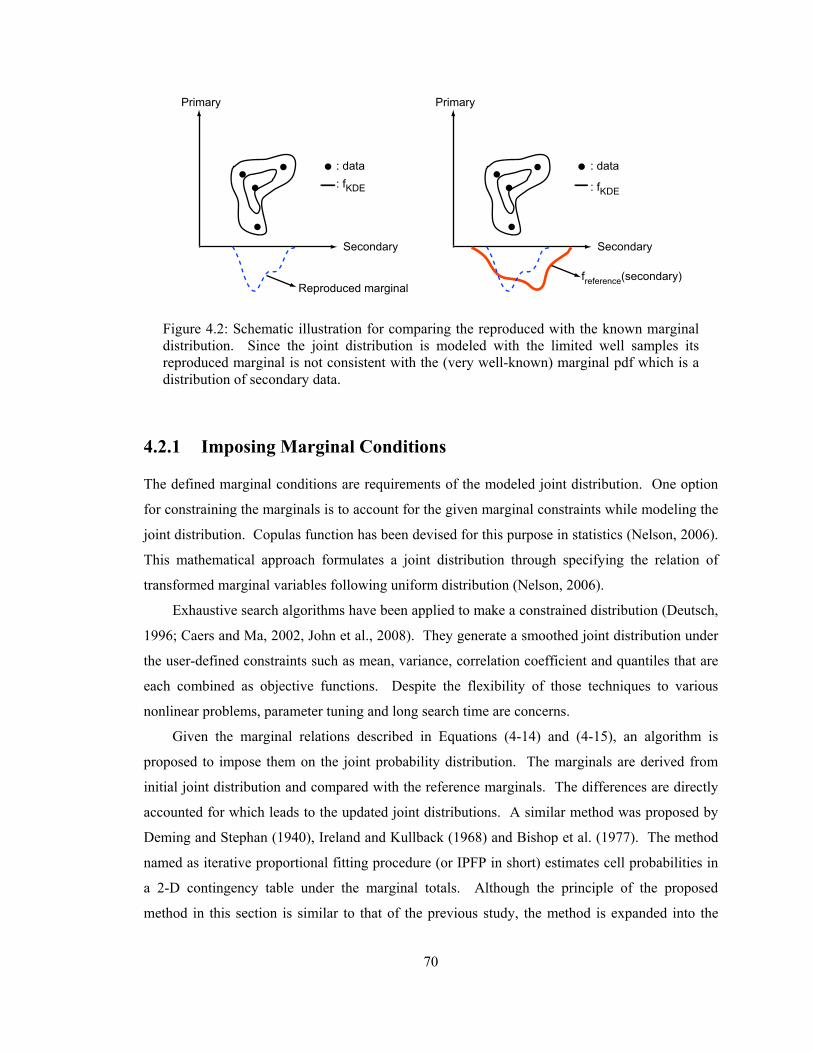
70

Figure 4.2: Schematic illustration for comparing the reproduced with the known marginal distribution. Since the joint distribution is modeled with the limited well samples its reproduced marginal is not consistent with the (very well-known) marginal pdf which is a distribution of secondary data.

4.2.1 Imposing Marginal Conditions

The defined marginal conditions are requirements of the modeled joint distribution. One option

for constraining the marginals is to account for the given marginal constraints while modeling the

joint distribution. Copulas function has been devised for this purpose in statistics (Nelson, 2006).

This mathematical approach formulates a joint distribution through specifying the relation of

transformed marginal variables following uniform distribution (Nelson, 2006).

Exhaustive search algorithms have been applied to make a constrained distribution (Deutsch,

1996; Caers and Ma, 2002, John et al., 2008). They generate a smoothed joint distribution under

the user-defined constraints such as mean, variance, correlation coefficient and quantiles that are

each combined as objective functions. Despite the flexibility of those techniques to various

nonlinear problems, parameter tuning and long search time are concerns.

Given the marginal relations described in Equations (4-14) and (4-15), an algorithm is

proposed to impose them on the joint probability distribution. The marginals are derived from

initial joint distribution and compared with the reference marginals. The differences are directly

accounted for which leads to the updated joint distributions. A similar method was proposed by

Deming and Stephan (1940), Ireland and Kullback (1968) and Bishop et al. (1977). The method

named as iterative proportional fitting procedure (or IPFP in short) estimates cell probabilities in

a 2-D contingency table under the marginal totals. Although the principle of the proposed

method in this section is similar to that of the previous study, the method is expanded into the

Primary

Secondary

: data: fKDE : fKDE

Primary

Secondary

: data

freference(secondary)Reproduced marginal

71

multidimensional problem with continuous variables. This correcting process is performed by the

following steps:

Step1. Model the joint distribution of secondary data, f(D1,…,Dm) and global distribution of

primary variable, p(s). Declustering is considered for obtaining an unbiased p(s) if required.

Step2. Model the joint distribution f(s,D1,…,Dm) and define it as f(0) to differentiate it from

the resulting joint distribution.

Step3. Scale the f(0) to ensure the marginal distribution shown in Equation (4-15). The

scaling equation below is proposed for ensuring the imposed marginal condition:

(0) (1)11 1(0)

11,...,

( ,..., )( , ,..., ) ( , ,..., )( , ,..., )

mm m

ms K

f D Df s D D f s D Df s D D

=

× →∑

(4-16)

The ratio f(D1,…,Dm)/Σs=1,…,K f(s,D1,…,Dm) is a modifying factor. If the marginal relation (4-

15) is satisfied then this factor becomes 1 leading to no changes in f(0). Otherwise, f(0) is

adjusted by the modifying factor that accounts for the differences between the reference

f(D1,…,Dm) and reproduced marginal distribution Σs=1,…,K f(s,D1,…,Dm). The corrected

distribution under one marginal condition is set as f(1) for the next step.

Step4. Scale the f(1) to ensure the marginal distribution shown in Equation (4-14). Similar to

the step 3, the scaling equation below is for updating the f(1):

(1) (2)1 1(1)

1 1

( )( , ,..., ) ( , ,..., )( , ,..., )m m

m m

p sf s D D f s D Df s D D dD dD

× →⋅⋅⋅ ⋅⋅ ⋅∫ ∫

(4-17)

The ratio p(s)/∫⋅⋅⋅∫f(1)(s,D1,…,Dm)dD1⋅⋅⋅dDm is another modifying factor. If the marginal

relation (4-14) is met then the factor becomes 1 leading to no change in f(1). Otherwise, f(1) is

adjusted by the modifying factor accounting for the differences between the reference

marginal distribution p(s) and the reproduced marginal distribution

∫⋅⋅⋅∫f(1)(s,D1,…,Dm)dD1⋅⋅⋅dDm . The corrected distribution under marginal condition (4-14) is

set as f(2).

Step5. Finish the procedure if the stopping rule is met, otherwise go to step 6.

Step6. Reset f(2) into f(0) and repeat steps 3 through 5.

Step 1 and 2 are initial steps to establish the marginal distributions p(s) and f(D1,…,Dm). p(s) is a

global distribution of the primary variable s constructed from well samples. f(D1,…,Dm) is m-

dimensional secondary data distribution. Steps 3 through 5 are employed to correct the initial

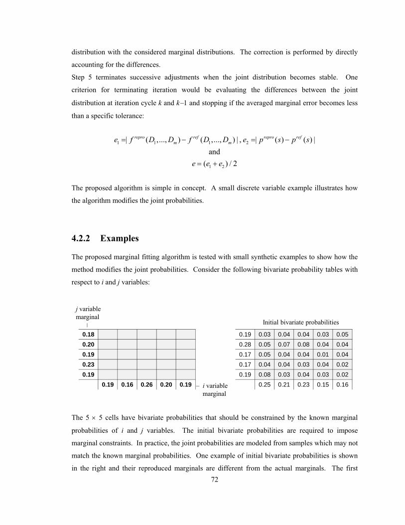
72

distribution with the considered marginal distributions. The correction is performed by directly

accounting for the differences.

Step 5 terminates successive adjustments when the joint distribution becomes stable. One

criterion for terminating iteration would be evaluating the differences between the joint

distribution at iteration cycle k and k−1 and stopping if the averaged marginal error becomes less

than a specific tolerance:

1 1 1 2

1 2

| ( ,..., ) ( ,..., ) | , | ( ) ( ) |and

( ) / 2

repro ref repro refm me f D D f D D e p s p s

e e e

= − = −

= +

The proposed algorithm is simple in concept. A small discrete variable example illustrates how

the algorithm modifies the joint probabilities.

4.2.2 Examples

The proposed marginal fitting algorithm is tested with small synthetic examples to show how the

method modifies the joint probabilities. Consider the following bivariate probability tables with

respect to i and j variables:

The 5 × 5 cells have bivariate probabilities that should be constrained by the known marginal

probabilities of i and j variables. The initial bivariate probabilities are required to impose

marginal constraints. In practice, the joint probabilities are modeled from samples which may not

match the known marginal probabilities. One example of initial bivariate probabilities is shown

in the right and their reproduced marginals are different from the actual marginals. The first

– i variablemarginal

Initial bivariate probabilities

0.180.200.190.230.19

0.19 0.16 0.26 0.20 0.19

0.19 0.03 0.04 0.04 0.03 0.050.28 0.05 0.07 0.08 0.04 0.040.17 0.05 0.04 0.04 0.01 0.040.17 0.04 0.04 0.03 0.04 0.020.19 0.08 0.03 0.04 0.03 0.02

0.25 0.21 0.23 0.15 0.16

j variablemarginal–

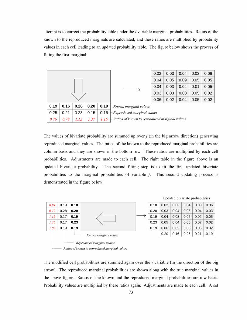
73

attempt is to correct the probability table under the i variable marginal probabilities. Ratios of the

known to the reproduced marginals are calculated, and these ratios are multiplied by probability

values in each cell leading to an updated probability table. The figure below shows the process of

fitting the first marginal:

The values of bivariate probability are summed up over j (in the big arrow direction) generating

reproduced marginal values. The ratios of the known to the reproduced marginal probabilities are

column basis and they are shown in the bottom row. These ratios are multiplied by each cell

probabilities. Adjustments are made to each cell. The right table in the figure above is an

updated bivariate probability. The second fitting step is to fit the first updated bivariate

probabilities to the marginal probabilities of variable j. This second updating process is

demonstrated in the figure below:

The modified cell probabilities are summed again over the i variable (in the direction of the big

arrow). The reproduced marginal probabilities are shown along with the true marginal values in

the above figure. Ratios of the known and the reproduced marginal probabilities are row basis.

Probability values are multiplied by these ratios again. Adjustments are made to each cell. A set

0.19 0.16 0.26 0.20 0.190.25 0.21 0.23 0.15 0.160.76 0.78 1.12 1.37 1.16

– Known marginal values– Reproduced marginal values

– Ratios of known to reproduced marginal values

0.02 0.03 0.04 0.03 0.060.04 0.05 0.09 0.05 0.050.04 0.03 0.04 0.01 0.050.03 0.03 0.03 0.05 0.020.06 0.02 0.04 0.05 0.02

0.94 0.19 0.180.72 0.28 0.201.15 0.17 0.191.36 0.17 0.231.03 0.19 0.19

Known marginal values

Reproduced marginal values

Ratios of known to reproduced marginal values

0.18 0.02 0.03 0.04 0.03 0.060.20 0.03 0.04 0.06 0.04 0.030.19 0.04 0.03 0.05 0.02 0.050.23 0.05 0.04 0.05 0.07 0.020.19 0.06 0.02 0.05 0.05 0.02

0.20 0.16 0.25 0.21 0.19

Updated bivariate probabilities

74

of horizontal and vertical comparison constitute one cycle for fitting the bivariate probabilities to

the known marginal probabilities. The updated bivariate probabilities shown in the right almost

exactly reproduce the true marginal probabilities. Initial bivariate probabilities are changed by 28%

on average after marginal correction. Another iteration could be performed with horizontal and

vertical summing and comparing with marginal values again: correction under the i variable

marginal probabilities and then correction under the j variable marginal probabilities. As iteration

proceeds (2nd, 3rd cycle and so on), the marginal errors will monotonically decrease (convergence

proof in section 4.3).

The 5×5 bivariate probability example demonstrates how the marginal fitting algorithm modifies

the initial probabilities at each iteration step. Figure 4.3 shows another example of applying the

algorithm to continuous variables. The initial bivariate pdf is modeled with samples. The

extracted univariate marginal distributions from the bivariate pdf do not agree with the true

marginal distributions. The extracted marginals and true marginals are shown as dashed and solid

lines, respectively. The bivariate pdf is corrected under the marginal constraints and exactly

reproduces the marginal distributions. The averaged marginal errors become 0.001% after 200

iterations.

Figure 4.3: The example of the marginal fitting algorithm for the continuous variable. Initial bivariate pdf is shown in the left. The actual marginal and reproduced marginal distributions are shown as sold and dashed lines, respectively. The fitting algorithm updates the initial pdf as shown in the right. Each marginal pdf is exactly reproduced.

75

The Effect of Initial Distributions

The proposed marginal fitting algorithm modifies the initial distribution to reproduce the fixed

marginal distributions that are projections of high dimensions on the lower dimensions. Multiple

solutions for joint distributions, therefore, are possible as long as they meet the lower dimensional

constraints. Figure 4.4 shows three different initial distributions and the resulting distributions

obtained by the marginal fitting procedure for consistent, uncorrelated and inconsistent cases.

The consistent case uses samples to model the initial distribution. The inconsistent case assumes

negative correlation. The true bivariate distribution is modeled with exhaustive samples and

shown in the right of Figure 4.4. The updated distributions generate the same accuracy of

marginal errors (e.g. 0.0001%) for three different initial guess; however, the final distributions are

different in shape. They preserve the overall relation of initial distribution: positive, uncorrelated

and negative bivariate relation. The algorithm cannot correct the inconsistency of the resulting

distribution despite satisfying marginal conditions. Fortunately, samples are available for the

multivariate distribution modeling and most cases that we face will be consistent cases.

76

Figure 4.4: The effect of the initial distributions when applying the algorithm. Three different cases generate different final bivariate distributions with the same accuracy of marginal errors.

4.3 Convergence of Sequential Marginal Fitting Algorithm

The considered method is based on the iterative procedure for matching the calculated marginals

to the fixed marginals. The final distribution should be stable and converge when iteration is

terminated. The algorithm guarantees a monotonic decreasing of the marginal errors. A small

discrete case is introduced to show convergence. The bivariate probabilities of RVs X and Y are

denoted as f(k)(xi,yj), i=1,2 and j=1,2, at kth iteration and they are assigned at four cell. The

univariate marginal probability densities are denoted as g(xi) and h(yj), i=1,2 and j=1,2. The

Uncorrelated case

Inconsistent case

Consistent case

Initial Updated

True

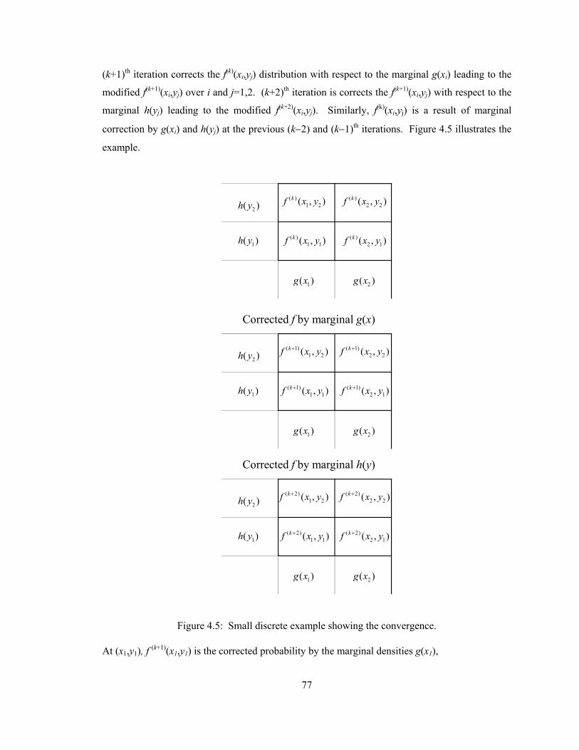
77

(k+1)th iteration corrects the f(k)(xi,yj) distribution with respect to the marginal g(xi) leading to the

modified f(k+1)(xi,yj) over i and j=1,2. (k+2)th iteration is corrects the f(k+1)(xi,yj) with respect to the

marginal h(yj) leading to the modified f(k+2)(xi,yj). Similarly, f(k)(xi,yj) is a result of marginal

correction by g(xi) and h(yj) at the previous (k−2) and (k−1)th iterations. Figure 4.5 illustrates the

example.

Figure 4.5: Small discrete example showing the convergence.

At (x1,y1), f (k+1)(x1,y1) is the corrected probability by the marginal densities g(x1),

( )1 1( , )kf x y ( )

2 1( , )kf x y

( )2 2( , )kf x y( )

1 2( , )kf x y2( )h y

1( )h y

1( )g x 2( )g x

( 1)1 1( , )kf x y+ ( 1)

2 1( , )kf x y+

( 1)2 2( , )kf x y+( 1)

1 2( , )kf x y+

2( )h y

1( )h y

1( )g x 2( )g x

( 2)1 1( , )kf x y+ ( 2)

2 1( , )kf x y+

( 2)2 2( , )kf x y+( 2)

1 2( , )kf x y+

2( )h y

1( )h y

1( )g x 2( )g x

Corrected f by marginal g(x)

Corrected f by marginal h(y)

78

( 1) ( )11 1 1 1( ) ( )

1 1 1 2

( )( , ) ( , )( , ) ( , )

k kk k

g xf x y f x yf x y f x y

+ =+

and f (k+2)(x1,y1) is the corrected probability by the marginal densities h(y1),

( 2) ( 1)11 1 1 1( 1) ( 1)

1 1 2 1

( )( , ) ( , )( , ) ( , )

k kk k

h yf x y f x yf x y f x y

+ ++ +=

+

Inserting f (k+1)(x1,y1) into f (k+2)(x1,y1) leads to the following,

( 2) 11 1

( ) ( )1 21 1 2 1( ) ( ) ( ) ( )

1 1 1 2 2 1 2 2

( )11 1( ) ( )

1 1 1 2

( )( , ) ( ) ( )( , ) ( , )( , ) ( , ) ( , ) ( , )

( ) ( , )( , ) ( , )

k

k kk k k k

kk k

h yf x y g x g xf x y f x yf x y f x y f x y f x y

g x f x yf x y f x y

+ = ×+

+ +

+where f(k+2)(x1,y1) is composed of the fixed marginal g(x) and h(y), and the probability corrected at

the previous kth iteration. f(k)(xi,yj) is a result from the correction of the f (k-2)(xi,yj) with respect to

the marginal g(x) and h(y), and thus the ratios g(x1)/{f(k)(x1,y1)+f(k)(x1,y2)} and

g(x2)/{f(k)(x2,y1)+f(k)(x2,y2)} are equal to 1. The f (k+2)(x1,y1) then becomes,

( 2) ( )11 1 1 1( ) ( )

1 1 2 1

( )( , ) ( , )( , ) ( , )

k kk k

h yf x y f x yf x y f x y

+ = ×+

whereas f(k)(x1,y1) is already corrected by the marginal densities h(yj) at (k−1)th iteration. Thus, the

ratio h(y1)/{f (k)(x1,y1)+f (k)(x2,y1)} becomes unity and f (k+2)(x1,y1) is identical to the f (k)(x1,y1). The

convergence of the |f (k+2)(x1,y1) – f (k)(x1,y1)|=0 will be reached if the marginal errors diminish.

The same proof can be applied to other cells (x1,y2), (x2,y1) and (x2,y2).

Convergence to Correct Distribution

The sequential algorithm updates the given distribution by the marginal constraints. As the

iteration proceeds, the marginal errors are decreased and the obtained distribution becomes stable

with no changes in probabilities. The convergence of the obtained distribution to the correct

distribution is proved. The modified joint distribution at kth and (k+1)th iteration steps can be

simply expressed by,

79

( ) ( 1) ( 1) ( ), , , ,( 1) ( )

, ,

andk k k kS PP S P S P S P Sk k

S P

f ff f f ff f

− +−

⋅ ⋅

= =

where the subscript P indicates the primary variable and S indicates a set of secondary variables.

fP and fS are marginal distributions of the primary and secondary variables deemed as a subset

derived from the correct joint distribution (*),P Sf . ( 1)

,kSf −

⋅ and ( ),k

Pf ⋅ are the reproduced marginals

from the obtained distribution at (k-1)th and kth steps over the primary and secondary variables,

respectively. To prove the convergence of ( ),k

P Sf and ( 1),k

P Sf + to (*),P Sf , Kullback-Leibler divergence

measure is used (Kullback, S. and Leibler, R.A., 1951). KL divergence is a measure of similarity

between two probability distributions. The measure is always non-negative and it is zero only if

two distributions are identical. KL divergence between the correct distribution (*),P Sf and the

obtained distribution ( ),k

P Sf at kth iteration step is,

(*),( ) (*)

, , ( ),,

log P SkP S P S k

P SP S

fD f

f⎛ ⎞

= ⎜ ⎟⎜ ⎟⎝ ⎠

∫

and it is expanded by,

( )

( ) ( ) ( ) ( )

(*),( ) (*)

, , ( ),,

(*) (*) (*) ( 1), , , , ( 1)

,,

(*) (*) (*) ( 1) (*) (*) ( 1), , , , , , ,

,

,(*),

,

log

log log

log log log log

log

P SkP S P S k

P SP S

k SP S P S P S P S k

SP S

k kP S P S P S P S P S S P S S

P S

P SP S

P S

fD f

f

ff f f ff

f f f f f f f f

ff

−−

⋅

− −⋅

⎛ ⎞= ⎜ ⎟⎜ ⎟

⎝ ⎠⎛ ⎞

= − ⋅⎜ ⎟⎜ ⎟⎝ ⎠

= − − +

=

∫

∫

∫

∫ ( ) ( )(*)

(*) (*) ( 1), , ,( 1)

, ,

log log kP S S P S Sk

P S P S

f f f ff

−⋅−

⎛ ⎞⎛ ⎞− −⎜ ⎟⎜ ⎟⎜ ⎟ ⎜ ⎟⎝ ⎠ ⎝ ⎠∫

The first integral term in the expansion above is KL divergence at (k-1)th step and thus,

80

( ) ( )

( ) ( )

( ) ( 1) (*) (*) ( 1), , , , ,

,

( 1) (*) (*) (*) ( 1) (*), , , , , ,

( 1) ( 1),

log log

log log where

k k kP S P S P S S P S S

P S

k kP S S S S S S S

S

k kP S S

D D f f f f

D f f f f f f

D D

− −⋅

− −⋅ ⋅ ⋅ ⋅ ⋅

− −

⎛ ⎞= − −⎜ ⎟⎜ ⎟

⎝ ⎠⎛ ⎞

= − − =⎜ ⎟⎝ ⎠

= −

∫

∫

Finally, KL divergence at kth step has the following relation with KL divergence at (k-1)th step,

( ) ( 1) ( 1), ,k k k

P S P S SD D D− −= −

Because the KL divergence is always non-negative, the following inequality holds,

( 1) ( 1) ( ) ( 1) ( ), , , ,0k k k k k

S P S P S P S P SD D D D D− − −= − ≥ ⇔ ≥ (4-18)

Similarly, the relation below is derived for kth and (k+1)th iteration,

( ) ( ) ( 1) ( ) ( 1), , , ,0k k k k k

P P S P S P S P SD D D D D+ += − ≥ ⇔ ≥ (4-19)

Equations (4-18) and (4-19) show that KL divergence is monotonically decreasing and the

sequential iteration makes the obtained joint distribution into the correct distribution.

The numerical experiments investigated in the next chapter show that the first few iterations

drastically drop the marginal errors and generate stable joint distributions.

81

Chapter 5

Applications of

Multivariate Distribution

Modeling

This chapter implements modeling the joint probability distribution under the specified

distribution constraints and demonstrates several applications of the methodology for reservoir

facies modeling through incorporating diverse data. Synthetic and field data are tested and results

are evaluated in terms of defined criteria.

Section 5.1 presents integration of secondary data for facies modeling. Mixtures of

continuous secondary and discrete primary variables are jointly modeled. The constraints for the

joint distributions are described. The marginal fitting algorithm discussed in Chapter 4 is applied

to correct the joint distribution. Seismic data or inverted seismic attributes typically have larger

scale than that of modeling cell or well data. The latter part of Section 5.1 illustrates how large

scale seismic data can be integrated and can provide facies proportions for relatively large

volumes.

Section 5.2 demonstrates the applicability of the joint modeling approach to debias global

facies proportions. Obtaining representative statistics is crucial to geostatistical reservoir

modeling, however, it is difficult to obtain unbiased statistics from the sparse well samples. This

section demonstrates the usefulness of incorporating the secondary data to obtain the

representative statistics through the modeling of joint relation.

82

Section 5.3 describes combining geologic analog information (or interpreted geologic map)

with multiple soft secondary information through joint modeling. Mixed joint distribution of

continuous and discrete variables is modeled in a nonparametric way and the marginal constraints

are imposed to obtain a corrected joint distribution.

This application demonstrates the value of the joint distribution modeling technique for

integrating different types of secondary and primary data. Nonparametric modeling enables us to

model the data distribution without distribution assumption, which accounts for the joint relation

among variables more realistically. The implemented marginal fitting algorithm makes the

modeled joint distribution legitimate at less computational burden.

5.1 Integrating Multiple Soft Secondary Data

Consider facies modeling conditioned to multiple secondary data. The joint probability

distribution of the primary facies and secondary variables is defined:

1( , ..., )mf s y y (5-1)

where s and Y=[y1,…,ym] are random variables representing discrete facies codes taking s=1,…,K

and continuous secondary data, respectively. If there are many secondary variables, for example

m ≥ 5, then aggregating those variables would be necessary by dimension reduction

preprocessing. Aggregated variables are to be considered as secondary variables for integration.

The conventional approach to joint probability distribution modeling of categorical and

continuous variables is to express it as a conditional distribution of continuous variables given the

values of the categorical variables, times the marginal probability of the latter which is a

probability of the categorical variable, for example f(y1,…,ym|s)p(s), s=1,…,K (Krzanowski, 1993).

The joint expression shown in Equation (5-1), however, is a more general form and it can provide

any lower order distributions by integrating any sub set of variables over the rest of variables,

which allows us to compare the lower order distributions with reference distributions. These

reference distributions are modeled from the exhaustive secondary data. K, the number of distinct

facies, is typically limited between 2 and 6. The facies become difficult to distinguish if they are

divided into more than 6 as the measured property distributions overlap. Once the joint

probability distribution f(s,y1,…,ym) is modeled, a conditional probability of facies given the

collocated secondary data at location u is immediately derived by the definition or a conditional

probability (Bayes relation):

83

11

1

( , ,..., )( | ,..., ) , 1,...,( ,..., )

mm

m

f s y yp s y y s Kf y y

= = (5-2)

5.1.1 Amoco Examples

The Amoco test data introduced in Chapter 3 are used again: the data set are extracted from a

West Texas Permian Basin reservoir and contain reservoir properties such as porosity and facies

types from 62 wells and exhaustively sampled seismic data over 10,400ft by 10,400ft area.

Porosities sampled at 62 well locations are simulated over the area to be treated as secondary data

in addition to the seismic data. Figure 5.1 shows cross plots of seismic and simulated porosity.

This cross plot shows that the considered secondary data has an ability to separate the two facies:

data points representing faces 1 (open circles) are located in the area of high porosity and seismic,

and points representing facies 2 (black circles) are located in the area of low porosity and seismic

values.

Figure 5.1: Cross plot of collocated secondary data.

The joint probability distribution of interest is f(s,y1,y2) and the marginal distributions of f(s,y1,y2)

must amount to p(s), s = 1,2 and f(y1,y2) where y1 and y2 represent porosity and seismic data. The

global probability (or proportion) p(s) are simply calculated by counting the corresponding

number from 62 samples: p(s=1) is 0.58=36/62 and p(s=2) is 0.42=26/62. Because of the cluster

of wells in the north-east corner, the representative proportions would be different from the naïve

proportions. Cell declustering was performed to mitigate the geometric clustering effect, and the

Y2

(sei

smic

)

Y1 (porosity)

Scatter plot of collocated secondary values

3.5 5.5 7.5 9.5 11.541000.

45000.

49000.

53000.

Number of data 62Overall corr = 0.62

84

declustered global proportions of facies are derived as p(s=1) = 0.514 and p(s=2) = 0.486

(Deutsch and Journel, 1998). The bivariate pdf of the secondary variables, f(y1,y2), is another

marginal distribution to constrain the joint distribution f(s,y1,y2). There are 4335 samples

available for f(y1,y2) modeling. Figure 5.2 shows the modeled f(y1,y2) by kernel density

estimation. The bivariate distribution could be assembled by directly sampling the frequency

from the 2-D histogram when the number of data is large (Doyen, 2007). The number of bins

where the bivariate densities are estimated is chosen as 50 and so the bivariate probability

densities are estimated at every 50 by 50 pixels in Figure 5.2.

Figure 5.2: The modeled bivariate distribution of secondary data f(y1,y2). The experimental 4225 data points are overlaid.

The 4225 data points are plotted with the smoothed bivariate distribution. The modeled

probability distribution reasonably honors the means, variance and correlation coefficient from

experimental data. The joint probability density function f(s,y1,y2) is modeled based on the 62

data. The joint pdf by the product kernel estimator is modeled by:

( )262

,1 2

1 11 2

1( , , ) w Imn

j j ii

i j j

y yf s y y s

nh h h

==

= =

⎛ ⎞⎛ ⎞−= ×⎜ ⎟⎜ ⎟⎜ ⎟⎜ ⎟× ⎝ ⎠⎝ ⎠

∑ ∏ (5-3)

where w(⋅) is a 1-D normal kernel function. This equation is a slightly modified equation from

the product kernel estimation shown in Equation (4-12). Since the primary variable is a discrete

variable not a continuous variable indicator function I(si) is added. The indicator function I(si)

takes 1 if facies from ith data out of n(=62) data corresponds to the facies code being modeled,

0.0

0.003

85

otherwise taking 0. For example, ns=1=36 samples out of 62 are used for modeling of f(s=1,y1,y2),

and ns=2=26 samples out of 62 are used for modeling of f(s=2,y1,y2). Equation (5-3) allows the

kernel estimation with the mixed continuous and discrete variables. Kernel bandwidth hj, j=1,2 is

set differently for different secondary variable. Figure 5.3 shows the modeled joint pdf before

being constrained by marginal conditions. Although the joint probability distributions are

modeled in 3-dimensional space (1 primary + 2 secondary variables), the distributions are clipped

and illustrated separately based on the facies variable for better visualizing and understanding.

Kernel bandwidths are chosen based on the relation 1( 4)ˆ , 1,2 and 2dj jh n j dσ − += = = (Scott,

1992).

Figure 5.3: The estimated joint probability distributions. The 3-D distribution is displayed separately for each facies category.

The bivariate distributions (clipped by facies code) reasonably reflect the experimental data

distributions. This reliance on data distribution is a strength of the nonparametric approach.

The modeled joint distributions should match the reference marginal distributions. The

marginal relations are for this example:

2

1 2 1 21

( , , ) ( , )s

f s y y f y y=

=∑ (5-4)

1 2 1 2( , , ) ( ), 1,2f s y y dy dy p s s= =∫ ∫ (5-5)

The left sides of above relations are the lower order distributions from the joint distribution. The

right sides are the reference distributions. The integration of f(s=1,y1,y2) and f(s=2,y1,y2) should

fSY(s=1,y1,y2) fSY(s=2,y1,y2)

Y1

Y2

Y1

Y2

0.0

0.003

86

amount to f(y1,y2), and totals of f(s=1,y1,y2) and f(s=2,y1,y2) over outcomes of (y1,y2) should

amount to p(s=1) and p(s=2), respectively. The sequential marginal fitting algorithm detailed in

Section 4.2 is applied to the initial joint distribution resulting in a corrected distribution that meets

all required marginal conditions. Figure 5.4 shows the corrected distributions constrained by

marginals using the algorithm. The unconstrained initial joint distributions are shown as well in

the left of the figure. Accounting for Equations (5-4) and (5-5) can be interpreted as adding up

the probability densities at every bins with the vertical direction and with horizontal direction in

Figure 5.4. The reproduced marginals and the reference marginals are compared in those

directions. The reproduced marginals from initial and corrected distributions are illustrated on

(y1,y2) plane (bottom), and on axis of the primary variable, respectively.

87

Figure 5.4: The joint probability distributions modeled by kernel estimator (left column) and modified distributions constrained by the imposed marginal conditions (right column). The arrow shown in the middle represents the direction of marginal fitting: two horizontal directions are to compare the probability of facies p(s), and vertical direction is to compare the secondary data distribution f(y1,y2).

Due to the richness of (y1,y2) samples and the reliability of f(y1,y2), detailed variations on

distributions are imparted to the corrected distributions. Areas of high porosity and high seismic

values (upper right corner) get high probability of facies 1 after marginal correction. The

probability of facies 2 increases around middle porosity and seismic value area (centre). These

changes have an impact on the final estimates of facies probability.

The corrected joint distributions are obtained after 20 marginal fitting iterations. Figure 5.5

shows the averaged marginal errors between empirical distributions and reference distributions

versus iteration numbers. The first few iterations drop the errors quickly and the averaged errors

become less than 0.1% before 8 iterations. Each iteration involves Bm+Bm×K arithmetic

operations and comparisons where B is number of bins, m is the number of secondary variables

and K is the number of categories. The first loop Bm is for fitting with the distribution of

secondary variables and the second loop Bm×K is for fitting with the probability of primary

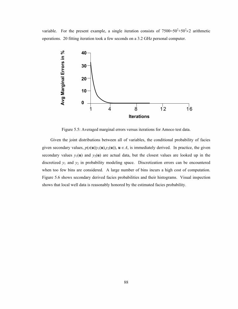
88

variable. For the present example, a single iteration consists of 7500=502+502×2 arithmetic

operations. 20 fitting iteration took a few seconds on a 3.2 GHz personal computer.

Figure 5.5: Averaged marginal errors versus iterations for Amoco test data.

Given the joint distributions between all of variables, the conditional probability of facies

given secondary values, p(s(u)|y1(u),y2(u)), u ∈A, is immediately derived. In practice, the given

secondary values y1(u) and y2(u) are actual data, but the closest values are looked up in the

discretized y1 and y2 in probability modeling space. Discretization errors can be encountered

when too few bins are considered. A large number of bins incurs a high cost of computation.

Figure 5.6 shows secondary derived facies probabilities and their histograms. Visual inspection

shows that local well data is reasonably honored by the estimated facies probability.

Iterations

0

20

10

30

40

Avg

Mar

gina

l Err

ors

in %

41 8 12 16

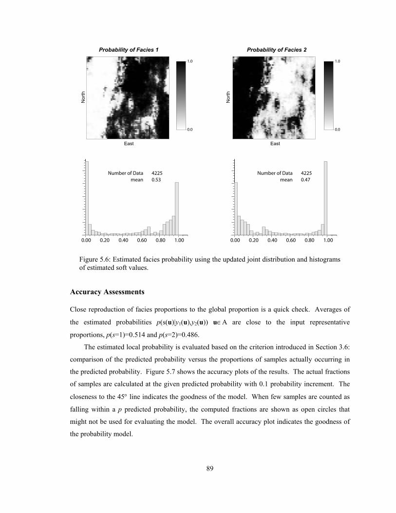
89

Figure 5.6: Estimated facies probability using the updated joint distribution and histograms of estimated soft values.

Accuracy Assessments

Close reproduction of facies proportions to the global proportion is a quick check. Averages of

the estimated probabilities p(s(u)|y1(u),y2(u)) u∈A are close to the input representative

proportions, p(s=1)=0.514 and p(s=2)=0.486.

The estimated local probability is evaluated based on the criterion introduced in Section 3.6:

comparison of the predicted probability versus the proportions of samples actually occurring in

the predicted probability. Figure 5.7 shows the accuracy plots of the results. The actual fractions

of samples are calculated at the given predicted probability with 0.1 probability increment. The

closeness to the 45° line indicates the goodness of the model. When few samples are counted as

falling within a p predicted probability, the computed fractions are shown as open circles that

might not be used for evaluating the model. The overall accuracy plot indicates the goodness of

the probability model.

Probability of Facies 1

East

Nor

th

East

Nor

th

0.0

1.0

Probability of Facies 2

0.0

1.0

0.00 0.20 0.40 0.60 0.80 1.00

Number of Datamean

42250.53

0.00 0.20 0.40 0.60 0.80 1.00

Number of Datamean

42250.47

90

Figure 5.7: Fairness plots of the local probabilities for the Amoco case. Actual fractions with few samples are shown as open circles and they are not used to evaluate the estimated local probability.

Building Stochastic Models

The derived faces probability from the given secondary data is integrated with indicator well data.

Sequential indicator simulation is performed using Bayesian updating equation to integrate the

secondary derived probability. The reasonableness of the generated realizations is checked with

the reproduction of variograms. Figure 5.8 shows the computed variograms from 21 realizations.

The effectiveness of integrating secondary data is observed by the small fluctuations in the

reproduced variograms.

Figure 5.8: The reproduced variograms in NS direction from 21 realizations: SISIM without secondary data (left) and with secondary derived probability that are obtained from the multivariate pdf modeling technique.

Act

ual f

ract

ion

Predicted prob0 0.2 0.4 0.6 0.8 1.0

0.0

0.2

0.4

0.6

0.8

1.0

Act

ual f

ract

ion

Predicted prob

Fairness plot for Facies 2Fairness plot for Facies 1 Fairness plot overall

0.0 0.2 0.4 0.6 0.8 1.00.0

0.2

0.4

0.6

0.8

1.0

Act

ual f

ract

ion

Predicted prob0.0 0.2 0.4 0.6 0.8 1.0

0.0

0.2

0.4

0.6

0.8

1.0

γ

Distance

SISIM

0. 1000. 2000. 3000. 4000. 5000. 6000.0.00

0.40

0.80

1.20

γ

Distance

SISIM with secondary data

0. 1000. 2000. 3000. 4000. 5000. 6000.0.00

0.40

0.80

1.20

91

5.1.2 West African Reservoir Example

Additional field data are tested with the proposed approach. A West African deepwater turbidite

reservoir is modeled with several seismic attributes. The reservoir is located in an average water

depth of 1,200ft and consists of stacked and amalgamated Micocene turbidite channel complex

that fills the steep canyons (Hoffman et. al., 2005). Vertically, individual meandering channels

exist within three stratigraphic units (Figure 5.9).

Figure 5.9: Interpreted stratigraphic units over the reservoir. Three massive bodies are interpreted with individual meandering channels. Four main facies are identified: high net-to-gross channel, sand, and low net-to-gross shale and shaly sand.

Four distinct facies are identified in core analysis: three sand facies with varying quality (coded 2

through 4) and a shale facies (coded 1). Sand facies represent a continuum of high, medium and

low net-to-gross (NTG). The area extends 5850m × 4425m × 696ft and the following grid is

defined over the area:

X Y Z Number of grids 78 59 116

Grid size 75m 75m 6ft

A total of 533,832 grid nodes are defined for the modeling, but only approximately 100,000 are

active. Seismic inversion provided high resolution seismic attributes in 3-D: acoustic impedance,

fraction of shale using three different inversion techniques and amplitude. All seismic attributes

depositionalflow direction

N

92

were provided as normalized units within [0,1]. Figure 5.10 shows 3-D sections of the first

seismic attribute with wells.

Figure 5.10: 3-D view of the first seismic attribute.

Figure 5.11 shows a histogram of the seismic attributes. The distribution of seismic variables 2

and 3 are almost the same distribution: very close mean, variance and quantiles each other.

Seismic variables 1 and 4 are distributed over the full range of [0,1], but seismic variable 5 is

limited by a maximum value of 0.34 with low variance.

N

900m

93

Figure 5.11: Distributions of seismic attributes sampled from well locations.

Table 5.1 summarizes the relations between seismic attributes (denoted as S1 ~ S5) and facies

types (F1 ~ F4). This descriptive statistics can provide the overall interpretation about the

redundancy and relevance among variables.

Table 5.1: Linear correlation among variables

Seismic 1 Seismic 2 Seismic 3 Seismic 4 Seismic 5 F1 F2 F3 F4 Seismic 1 1.0 -0.25 -0.05 0.31 0.06 0.34 0.01 -0.08 -0.31 Seismic 2 1.0 0.91 -0.07 0.57 0.07 -0.06 -0.03 -0.02 Seismic 3 1.0 0.01 0.53 0.09 -0.03 -0.04 -0.05 Seismic 4 1.0 0.09 0.20 0.02 -0.03 -0.21 Seismic 5 1.0 0.25 -0.09 -0.02 -0.2

Seismic variables 2 and 3 have weak correlations with all facies types. Seismic variables 1, 4 and

5 are somewhat correlated to facies 1 and 4, but barely correlated to facies 2 and 3. Based on the

summary of correlation and histograms, seismic variables 1, 4 and 5 can be candidates for

secondary variables to be integrated. The key idea is to choose seismic attributes that maximize

the correlation between the seismic and facies, and minimize the correlation between the seismic

themselves. Seismic 1 and 5 (noted as RVs Y1 and Y2 hereafter) are chosen since they are more

related to facies and less related to each other. One may assume that the magnitude of correlation

between the considered seismic and facies does not seem to be high enough. Integrating diverse

data, however, could make features unseen in the individual data emerge and thus secondary data

with small correlations to the primary data are worth to be considered unless zero correlations are

Seismic 10.0 0.2 0.4 0.6 0.8 1.0

Seismic 40.0 0.2 0.4 0.6 0.8 1.0

Seismic 50.0 0.2 0.4 0.6 0.8 1.0

Seismic 20.0 0.2 0.4 0.6 0.8 1.0

Seismic 30.0 0.2 0.4 0.6 0.8 1.0

0.000.010.020.030.040.050.060.07

0.00

0.04

0.08

0.12

0.00

0.04

0.08

0.12

0.00

0.01

0.02

0.03

0.04

0.05

0.0

0.1

0.2

0.3

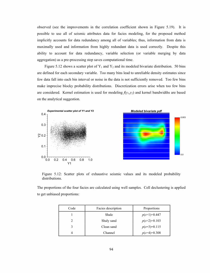
94

observed (see the improvements in the correlation coefficient shown in Figure 5.19). It is

possible to use all of seismic attributes data for facies modeling, for the proposed method

implicitly accounts for data redundancy among all of variables; thus, information from data is

maximally used and information from highly redundant data is used correctly. Despite this

ability to account for data redundancy, variable selection (or variable merging by data

aggregation) as a pre-processing step saves computational time.

Figure 5.12 shows a scatter plot of Y1 and Y2 and its modeled bivariate distribution. 50 bins

are defined for each secondary variable. Too many bins lead to unreliable density estimates since

few data fall into each bin interval or noise in the data is not sufficiently removed. Too few bins

make imprecise blocky probability distributions. Discretization errors arise when too few bins

are considered. Kernel estimation is used for modeling f(y1,y2) and kernel bandwidths are based

on the analytical suggestion.

Figure 5.12: Scatter plots of exhaustive seismic values and its modeled probability distributions.

The proportions of the four facies are calculated using well samples. Cell declustering is applied

to get unbiased proportions:

Code Facies description Proportions

1 Shale p(s=1)=0.447

2 Shaly sand p(s=2)=0.103

3 Clean sand p(s=3)=0.115

4 Channel p(s=4)=0.308

Y2

Y1

Experimental scatter plot of Y1 and Y2

0.0 0.2 0.4 0.6 0.8 1.00.0

0.1

0.2

0.3

0.4Modeled bivariate pdf

0.0

0.003

95

The prepared f(y1,y2) and p(s) are marginal constraints that f(s,y1,y2) must consider. It is good

practice to plot experimental data points before inferring the joint distribution. Figure 5.13 shows

scatter plots of the selected seismic variables depending on different facies types. If the seismic

data have good capability of identifying facies, then the data points will fall in distant groups.

For this example, the scatter plots of mean values are shown in the bottom of Figure 5.13. Means

of (Y1,Y2) for facies 2 and 3 closely overlap and means of (Y1,Y2) for facies 1 and 4 are

somewhat separated. The chosen seismic data helps identify shale (F1) and channel facies (F4),

and does not help recognize intermediate sand facies (F2 and F3). This results from the weak

correlation of the selected seismic attribute 1 and 5 to the facies 2 and 3.

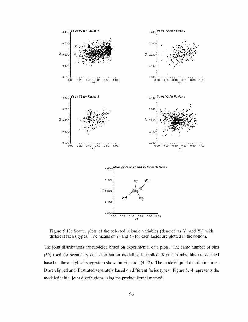
96

Figure 5.13: Scatter plots of the selected seismic variables (denoted as Y1 and Y2) with different facies types. The means of Y1 and Y2 for each facies are plotted in the bottom.

The joint distributions are modeled based on experimental data plots. The same number of bins

(50) used for secondary data distribution modeling is applied. Kernel bandwidths are decided

based on the analytical suggestion shown in Equation (4-12). The modeled joint distribution in 3-

D are clipped and illustrated separately based on different facies types. Figure 5.14 represents the

modeled initial joint distributions using the product kernel method.

Y2

Y1

Y1 vs Y2 for Facies 1

0.00 0.20 0.40 0.60 0.80 1.000.000

0.100

0.200

0.300

0.400

Y2

Y1

Y1 vs Y2 for Facies 2

0.00 0.20 0.40 0.60 0.80 1.000.000

0.100

0.200

0.300

0.400

Y2

Y1

Y1 vs Y2 for Facies 3

0.00 0.20 0.40 0.60 0.80 1.000.000

0.100

0.200

0.300

0.400

Y2

Y1

Y1 vs Y2 for Facies 4

0.00 0.20 0.40 0.60 0.80 1.000.000

0.100

0.200

0.300

0.400

F1F2

F3F4

Y2

Y1

Mean plots of Y1 and Y2 for each facies

0.00 0.20 0.40 0.60 0.80 1.000.000

0.100

0.200

0.300

0.400

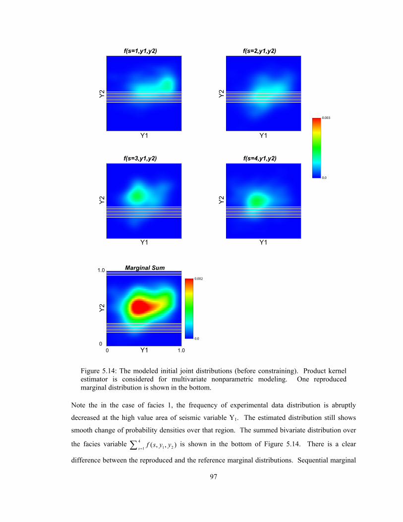
97

Figure 5.14: The modeled initial joint distributions (before constraining). Product kernel estimator is considered for multivariate nonparametric modeling. One reproduced marginal distribution is shown in the bottom.

Note the in the case of facies 1, the frequency of experimental data distribution is abruptly

decreased at the high value area of seismic variable Y1. The estimated distribution still shows

smooth change of probability densities over that region. The summed bivariate distribution over

the facies variable 41 21

( , , )s

f s y y=∑ is shown in the bottom of Figure 5.14. There is a clear

difference between the reproduced and the reference marginal distributions. Sequential marginal

f(s=1,y1,y2) f(s=2,y1,y2)

f(s=3,y1,y2) f(s=4,y1,y2)

0.0

0.002

0.0

0.003

Marginal Sum

Y1

00

1.0

1.0

Y2

Y2

Y2

Y2

Y1

Y1

Y2

Y1

Y1

98

fitting procedure was applied to correct the differences. The modified joint distributions become

stable after 15 iterations in which averaged marginal errors reach less than 0.003%. Figure 5.15

shows the corrected distributions. For this example, each iteration involves 12,500=502+502×4

arithmetic calculations. The modified version show detailed variations in density distribution and

reasonably reflect experimental data scatter plots. The corrected distribution f(s=1,y1,y2) accounts

for the abrupt decrease in experimental data frequency over high value area of Y1.

Figure 5.15: The corrected joint distribution f(s,y1,y2) after applying marginal constraints.

0.

0.002

0.

0.003

Marginal Sum

Corrected f(s=1,y1,y2) Corrected f(s=2,y1,y2)

Corrected f(s=3,y1,y2) Corrected f(s=4,y1,y2)

Y1

Y2

Y2

Y2

Y2

Y1

Y1

Y2

Y1

Y1

00

1.0

1.0

99

The initial joint distributions have different shape with different choices of kernel

bandwidths. A small exercise is performed to check the marginal relation without updating.

Based on the optimal suggestion of kernel bandwidth 1( 4)ˆ , 1,2 and 2dj jh n j dσ − += = = , up to ±

60% changes in hj are tested. For each case of the initial joint distribution, the marginal

distribution f(y1,y2) is reproduced by the relation of 41 21

( , , )s

f s y y=∑ . Figure 5.16 illustrates the

calculated marginal distributions from the initial distributions that are modeled by kernel method

with different hj. None of initial distributions reproduce the marginal distribution correctly.

Figure 5.16: The joint distributions modeled with different conditions of kernel bandwidths. Based on theoretical kernel bandwidth hopt, 60% changes are applied.

At every modeling locations u∈A, the conditional probability of facies given the seismic

values is derived from the corrected joint distribution:

h = hopt x 0.4 h = hopt x 0.7 h = hopt x 0.85

h = hopt x 1.5 h = hopt x 1.3 h = hopt x 1.6

Reference

0.0

0.002

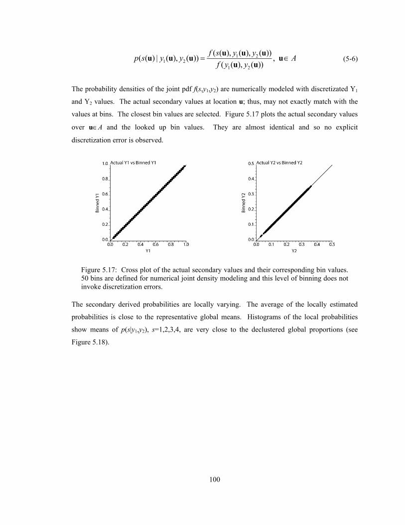
100

1 21 2

1 2

( ( ), ( ), ( ))( ( ) | ( ), ( )) ,( ( ), ( ))

f s y yp s y y Af y y

= ∈u u uu u u u

u u (5-6)

The probability densities of the joint pdf f(s,y1,y2) are numerically modeled with discretizated Y1

and Y2 values. The actual secondary values at location u; thus, may not exactly match with the

values at bins. The closest bin values are selected. Figure 5.17 plots the actual secondary values

over u∈A and the looked up bin values. They are almost identical and so no explicit

discretization error is observed.

Figure 5.17: Cross plot of the actual secondary values and their corresponding bin values. 50 bins are defined for numerical joint density modeling and this level of binning does not invoke discretization errors.

The secondary derived probabilities are locally varying. The average of the locally estimated

probabilities is close to the representative global means. Histograms of the local probabilities

show means of p(s|y1,y2), s=1,2,3,4, are very close to the declustered global proportions (see

Figure 5.18).

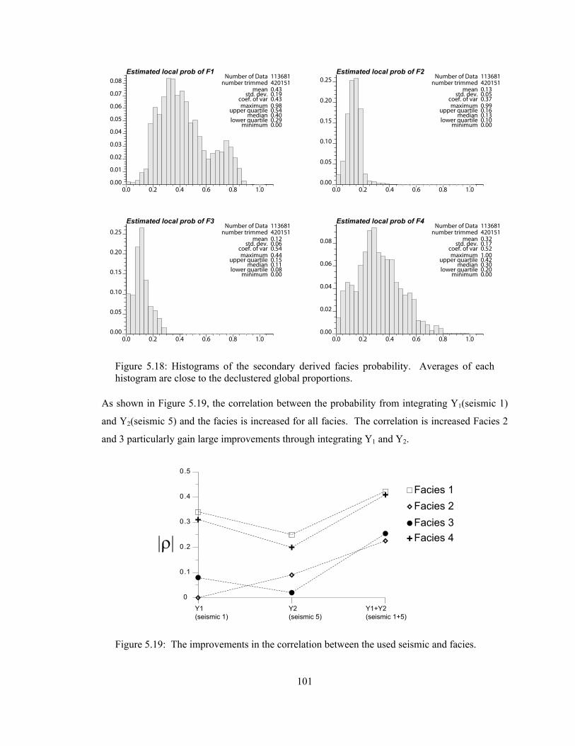
101

Figure 5.18: Histograms of the secondary derived facies probability. Averages of each histogram are close to the declustered global proportions.

As shown in Figure 5.19, the correlation between the probability from integrating Y1(seismic 1)

and Y2(seismic 5) and the facies is increased for all facies. The correlation is increased Facies 2

and 3 particularly gain large improvements through integrating Y1 and Y2.

Figure 5.19: The improvements in the correlation between the used seismic and facies.

0.0 0.2 0.4 0.6 0.8 1.00.00

0.01

0.02

0.03

0.04

0.05

0.06

0.07

0.08Estimated local prob of F1

Number of Data 113681number trimmed 420151

mean 0.43std. dev. 0.19

coef. of var 0.43maximum 0.98

upper quartile 0.54median 0.40

lower quartile 0.29minimum 0.00

0.0 0.2 0.4 0.6 0.8 1.00.00

0.05

0.10

0.15

0.20

0.25Estimated local prob of F2

Number of Data 113681number trimmed 420151

mean 0.13std. dev. 0.05

coef. of var 0.37maximum 0.99

upper quartile 0.16median 0.13

lower quartile 0.10minimum 0.00

0.0 0.2 0.4 0.6 0.8 1.00.00

0.05

0.10

0.15

0.20

0.25

Estimated local prob of F3Number of Data 113681

number trimmed 420151mean 0.12

std. dev. 0.06coef. of var 0.54maximum 0.44

upper quartile 0.15median 0.11

lower quartile 0.08minimum 0.00

0.0 0.2 0.4 0.6 0.8 1.00.00

0.02

0.04

0.06

0.08

Estimated local prob of F4Number of Data 113681

number trimmed 420151mean 0.32

std. dev. 0.17coef. of var 0.52maximum 1.00

upper quartile 0.42median 0.30

lower quartile 0.20minimum 0.00

Y1(seismic 1)

Y2(seismic 5)

Y1+Y2(seismic 1+5)

0

0.1

0.2

0.3

0.4

0.5

|ρ|

Facies 2Facies 3

Facies 1

Facies 4

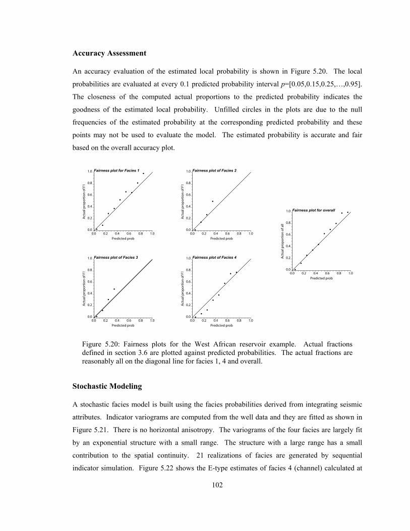
102

Accuracy Assessment

An accuracy evaluation of the estimated local probability is shown in Figure 5.20. The local

probabilities are evaluated at every 0.1 predicted probability interval p=[0.05,0.15,0.25,…,0.95].

The closeness of the computed actual proportions to the predicted probability indicates the

goodness of the estimated local probability. Unfilled circles in the plots are due to the null

frequencies of the estimated probability at the corresponding predicted probability and these

points may not be used to evaluate the model. The estimated probability is accurate and fair

based on the overall accuracy plot.

Figure 5.20: Fairness plots for the West African reservoir example. Actual fractions defined in section 3.6 are plotted against predicted probabilities. The actual fractions are reasonably all on the diagonal line for facies 1, 4 and overall.

Stochastic Modeling

A stochastic facies model is built using the facies probabilities derived from integrating seismic

attributes. Indicator variograms are computed from the well data and they are fitted as shown in

Figure 5.21. There is no horizontal anisotropy. The variograms of the four facies are largely fit

by an exponential structure with a small range. The structure with a large range has a small

contribution to the spatial continuity. 21 realizations of facies are generated by sequential

indicator simulation. Figure 5.22 shows the E-type estimates of facies 4 (channel) calculated at

Act

ual p

ropo

rtio

n of

F1

Predicted prob

Fairness plot for Facies 1

0.0 0.2 0.4 0.6 0.8 1.00.0

0.2

0.4

0.6

0.8

1.0

Act

ual p

ropo

rtio

n of

F1

Predicted prob

Fairness plot of Facies 2

0.0 0.2 0.4 0.6 0.8 1.00.0

0.2

0.4

0.6

0.8

1.0

Act

ual p

ropo

rtio

n of

F1

Predicted prob

Fairness plot of Facies 3

0.0 0.2 0.4 0.6 0.8 1.00.0

0.2

0.4

0.6

0.8

1.0

Act

ual p

ropo

rtio

n of

F1

Predicted prob

Fairness plot of Facies 4

0.0 0.2 0.4 0.6 0.8 1.00.0

0.2

0.4

0.6

0.8

1.0 Act

ual p

ropo

rtio

n of

all

Predicted prob

Fairness plot for overall

0.0 0.2 0.4 0.6 0.8 1.00.0

0.2

0.4

0.6

0.8

1.0

103

every modeling grids from 21 simulated facies. The sinuosity of channel is not well detected in

the E-type estimate and the connectivity of channel is not reproduced properly.

The seismic derived facies probability is now integrated. The Bayesian updating equation is used

to build the local conditional probability using the well data and the estimated facies probability

from seismic data. The E-type estimate is also calculated from 21 realizations and it is shown in

Figure 5.23. The meandering channel pattern is better identified and channel connectivity

interpreted in the conceptual geology in Figure 5.9 is revealed more clearly. The validity of the

stochastic models is based on the reasonable reproduction of the input statistics such as the input

variogram: low fluctuation of the reproduced variogram being close to the input model is ideal.

Figure 5.24 shows the reproduced variograms for the four facies at each principal direction.

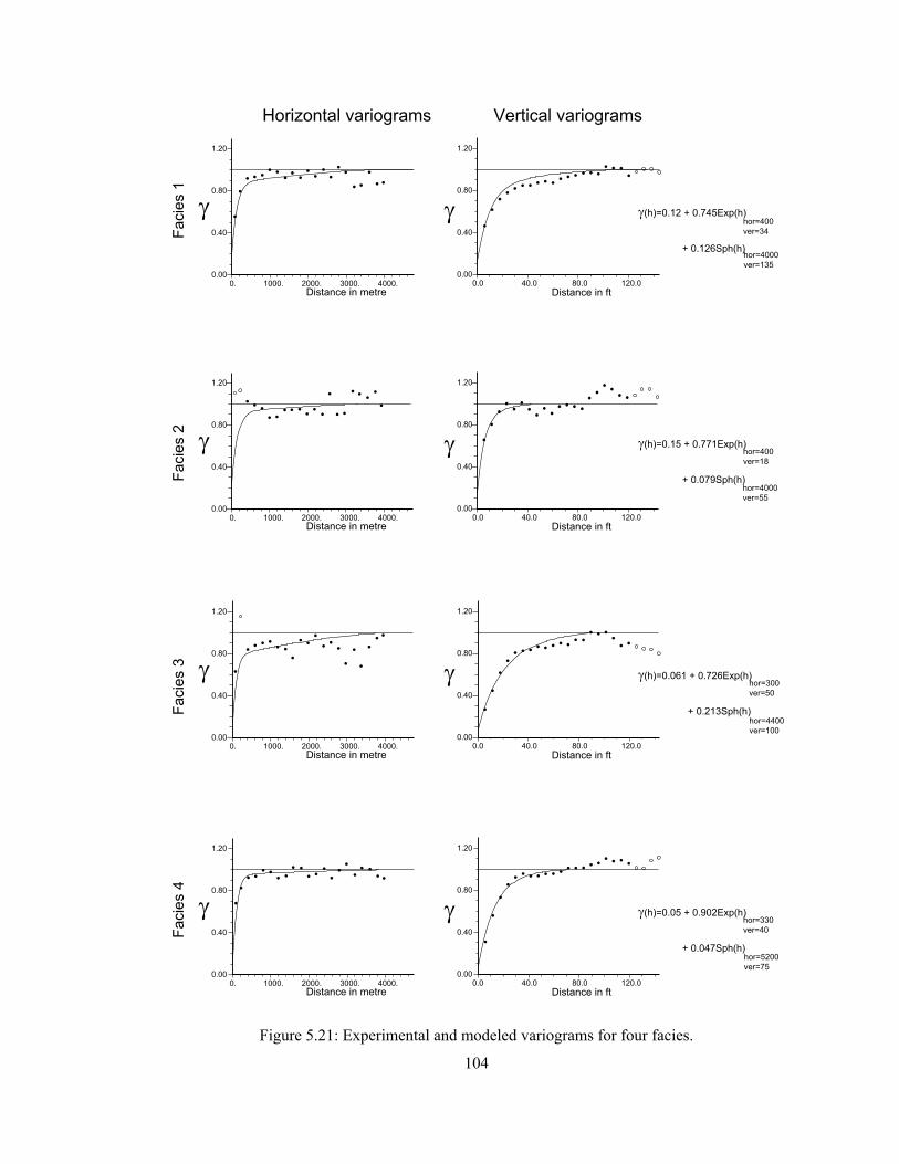
104

Figure 5.21: Experimental and modeled variograms for four facies.

Horizontal variograms Vertical variograms

Faci

es 1

γ

0. 1000.Distance in metre

2000. 3000. 4000.0.00

0.40

0.80

1.20

γ

Distance in ft0.0 40.0 80.0 120.0

0.00

0.40

0.80

1.20

Faci

es 2 γ

0. 1000.Distance in metre

2000. 3000. 4000.0.00

0.40

0.80

1.20

Distance in ft0.0 40.0 80.0 120.0

0.00

0.40

0.80

1.20

γ

Faci

es 3 γ

0. 1000.Distance in metre

2000. 3000. 4000.0.00

0.40

0.80

1.20

Distance in ft0.0 40.0 80.0 120.0

0.00

0.40

0.80

1.20

γ

Faci

es 4

γ

0. 1000.Distance in metre

2000. 3000. 4000.0.00

0.40

0.80

1.20

γ

Distance in ft0.0 40.0 80.0 120.0

0.00

0.40

0.80

1.20

γ(h)=0.12 + 0.745Exp(h) + 0.126Sph(h)

hor=400ver=34

hor=4000ver=135

γ(h)=0.15 + 0.771Exp(h)

+ 0.079Sph(h)

hor=400ver=18

hor=4000ver=55

γ(h)=0.061 + 0.726Exp(h)

+ 0.213Sph(h)

hor=300ver=50

hor=4400ver=100

γ(h)=0.05 + 0.902Exp(h)

+ 0.047Sph(h)

hor=330ver=40

hor=5200ver=75

105

Figure 5.22: E-type estimate of channel facies from 21 realizations without secondary data.

Figure 5.23: E-type estimate of channel facies from 21 realizations with secondary data.

layer 48

XY XZ YZ

layer 27

layer 34

layer 46

layer 56

layer 84

0.0

1.0

layer 48

XY XZ YZ

layer 27

layer 34

layer 46

layer 56

layer 84

0.0

1.0

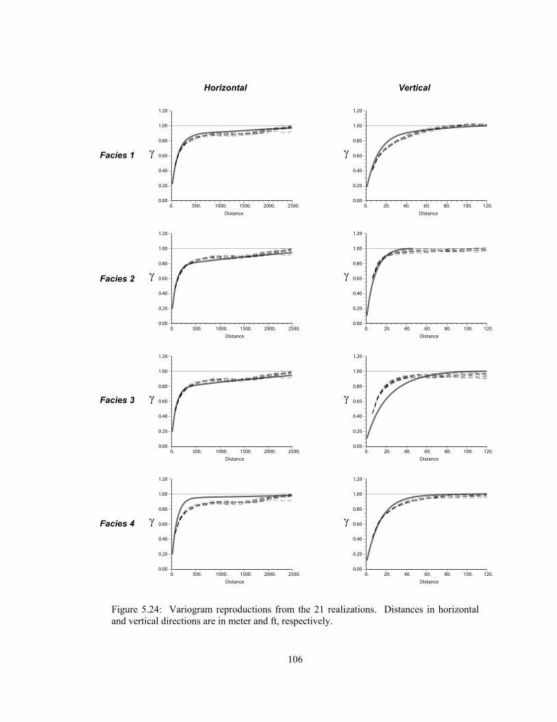
106

Figure 5.24: Variogram reproductions from the 21 realizations. Distances in horizontal and vertical directions are in meter and ft, respectively.

γ

Distance0. 500. 1000. 1500. 2000. 2500.

0.00

0.20

0.40

0.60

0.80

1.00

1.20

γ

Distance

Horizontal

Facies 1

Facies 2

Facies 3

Facies 4

Vertical

0. 20. 40. 60. 80. 100. 120.0.00

0.20

0.40

0.60

0.80

1.00

1.20

γ

Distance0. 500. 1000. 1500. 2000. 2500.

0.00

0.20

0.40

0.60

0.80

1.00

1.20

γ

Distance0. 20. 40. 60. 80. 100. 120.

0.00

0.20

0.40

0.60

0.80

1.00

1.20

γ

Distance0. 500. 1000. 1500. 2000. 2500.

0.00

0.20

0.40

0.60

0.80

1.00

1.20

γ

Distance0. 20. 40. 60. 80. 100. 120.

0.00

0.20

0.40

0.60

0.80

1.00

1.20

γ

Distance0. 500. 1000. 1500. 2000. 2500.

0.00

0.20

0.40

0.60

0.80

1.00

1.20

γ

Distance0. 20. 40. 60. 80. 100. 120.

0.00

0.20

0.40

0.60

0.80

1.00

1.20

107

5.1.3 Accounting for Large Scale Secondary Data

It is important to integrate information from seismic data that delivers better areal coverage than

the sparse sampling of well data. Seismic data, however, inexactly measures facies proportions

because of geological complications and inherent limitations in seismic data acquisition (Deutsch,

1996). Poor vertical resolution of the seismic data warrants using a single 2D map representing

vertically averaged facies proportions and the vertical volume is significantly larger than the

typical geological modeling cell.

The developed method to integrate soft secondary data can be applied for integrating large

scaled seismic data. The detailed process follows that described in Chapter 4: (1) model the

secondary data distribution which is a distribution of block values in this case and get the

representative global facies proportions, (2) model the joint distribution using kernel density

estimation, (3) constrain the joint distribution to the joint distribution of the secondary data and

the representative proportions, and (4) derive the conditional probabilities from the corrected joint

distribution.

Figure 5.25 shows a synthetic reference image consisting of three facies types and selected

wells from a reference image. The example is a vertical section of the reservoir with size of

100m in lateral and 50m in vertical direction. The modeling cell size is 1m-by-1m in horizontal

and vertical direction.

108

Figure 5.25: A synthetic reference images and well data extracted from the reference image. Coordinates are all in meter.

Two soft secondary variables are simulated. The vertical resolution of the secondary data is

assumed to be 5 times larger than the modeling size and so secondary values are generated at

every 1m in horizontal and 5m in vertical. Figure 5.26 shows the prepared secondary data.

Sequential Gaussian simulation was used for generating secondary data and they are non-linearly

correlated.

Reference image

EastD

epth

0 1000

50

F1

F2

F3

W-1 W-2 W-3 W-4 W-5W-6

0 20 40 60 80 1000

10

20

30

40

50

109

Figure 5.26: Two simulated secondary data. Vertical resolution is 5 times larger than the modeling cell size. Kernel method is used for the modeling of bivariate relation.

Figure 5.27 shows cross plots of block secondary values and facies proportions calculated from

well data.

Figure 5.27: Cross plots of block secondary values and facies proportions from 6 vertical wells.

The magnitude of correlation between the secondary data and the proportions varies from 0.3 to

0.8. Simulated secondary Y1(u) has an intermediate positive correlation (approximately 0.5) to

facies 2 and 3 but high negative correlation to the facies 1. Secondary Y2(u) has a low-to-

Simulated Secondary 1

East

Dep

th

0 1000

50

-2.0

0.0

2.0 2.0

2.0-2.0 Y1

Y2

-2.0

Joint pdf f(y1,y2)

0.0

0.002

Simulated Secondary 2

East

Dep

th

0 1000

50

Block values of S1 vs S2 Block S1 vs Proportions of F1 Block S1 vs Proportions of F2 Block S1 vs Proportions of F3

Block S2 vs Proportions of F1 Block S2 vs Proportions of F2 Block S2 vs Proportions of F3

-2-2

1

1 -2 1-2 1-20

1

0

1

0

1

0

1

-2 1-2 1-2 1

1

0

1

0

ρ = −0.189ρrank= −0.354

ρ = −0.803ρrank= −0.855

ρ = 0.481ρrank= 0.688

ρ = 0.448ρrank= 0.599

ρ = 0.422ρrank= 0.498

ρ = 0.295ρrank= 0.338

ρ = −0.798ρrank= −0.796

110

intermediate positive correlation to the facies 1 and 2 but high negative correlation to the facies 3,

which represents secondary data Y2(u) would better identify facies 3 from facies 1 and 2.

The two secondary data have a different capability of identifying different facies. This will show

how the integration results benefit from the full use of complementary information.

Figure 5.28 shows the comparison of the facies proportions calculated from block average of

the reference image and the secondary derived proportions. The scatter plot shows that the

estimated proportions using the joint distribution modeling technique are in consistent with the

true proportions.

Y1

Facies 1

Facies 2

Facies 3

Y2

Facies 1

Facies 2

Facies 3

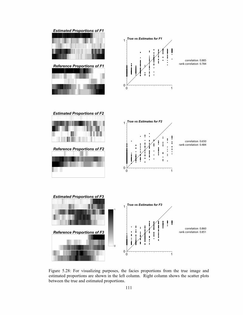
111

Figure 5.28: For visualizing purposes, the facies proportions from the true image and estimated proportions are shown in the left column. Right column shows the scatter plots between the true and estimated proportions.

Estimated Proportions of F1

Reference Proportions of F1correlation 0.885

rank correlation 0.784

True vs Estimates for F1

Estimated Proportions of F2

Reference Proportions of F2

correlation 0.650rank correlation 0.484

True vs Estimates for F2

Estimated Proportions of F3

Reference Proportions of F3

0

1

correlation 0.860rank correlation 0.851

True vs Estimates for F3

0 1

0 1

0 1

1

0

1

0

1

0

112

Comparing to the experimental scatter plots, the strength of correlation increases after data

integration. For example, each secondary data 1 and 2 has low correlation to the proportion of

facies 2 (less than 0.5 for both secondary) but integrated proportions of facies 2 have a correlation

of 0.65 that increases by 35%. Besides, even though two secondary data each has opposite

correlation to facies 1 and 3 (for example, ρY1F1= –0.803, ρY2F1=–0.422 and ρY1F3=0.448, ρY2F3 = –

0.798), the integrated results have higher correlations to the facies 1 and 3 rather than individual

correlations. This incremental improvement of information is the main advantage of data

integration when the integration model is valid in terms of reasonable accounting for data

redundancy and closeness.

Averages of the estimated proportions reasonably reproduce the global proportions. Figure 5.29

shows histograms of the estimated facies proportions. Note that the average of estimated

proportions is highly close to the global proportions.

113

Figure 5.29: Histograms of secondary derived facies proportions. Averages of each facies proportions are very close to the global representative facies proportions.

Estimated Prob of F10.00 0.20 0.40 0.60 0.80 1.00

0.000

0.040

0.080

0.120mean 0.41

Estimated Prob of F20.00 0.20 0.40 0.60 0.80 1.00

0.000

0.100

0.200

0.300mean 0.21

Estimated Prob of F30.00 0.20 0.40 0.60 0.80 1.00

0.000

0.040

0.080

0.120

0.160 mean 0.37

Code1 2 3

0.0

0.1

0.2

0.3

0.4

Global Facies Proportions from Well Data

114

5.2 Debiasing with Multiple Soft Secondary Data

Geostatistical models must reproduce the input statistics and spatial continuity; however, there is

no intrinsic declustering or debiasing in geostatistical modeling methods. Sample clustering

occurs when the domain of interest is sampled preferentially. It is natural that spatial data are

collected in a non-representative way such as preferential drilling in high net-to-gross area.

As discussed in Section 2.2.5, declustering techniques are widely used techniques for

correcting potentially biased sample statistics. Various types of declustering methods such as cell,

polygonal and kriging weight declustering have been developed (Deutsch and Journel, 1998;

Isaaks and Srivastava, 1989). Those techniques try to correct the bias inherent in sample statistics

caused by geometric clustering.

A debiasing algorithm uses quantitative secondary data for correcting the bias inherent in

samples. Soft secondary data may be representative of the entire area of interest, and the relation

between the primary variable being predicted and secondary data is modeled. The joint

probability distribution describes this relation. The central idea of debiasing is to extrapolate the

primary distributions over the full range of the secondary values. For example, the global facies

proportions can be debiased with respect to the secondary data distribution such as:

( ) ( , )debiasp s f s d∞

−∞= ∫ y y (5-7)

where the f(s,y) is the modeled joint distribution that satisfies all the axioms of a joint pdf:

positive densities, S ( , )s

f s d∀∑ ∫ Y y y = 1 and reproduction of lower order marginal distribution.

The use of a linear assumption among secondary variables is straightforward. Challenges are to

use secondary data accounting for non-Gaussian relations among them. The proposed debiasing

approach with soft secondary data is based on three steps: (1) build the joint distribution of all

secondary variables, build the initial joint distribution of the primary and all of secondary

variables, (2) correct the initial distributions under the secondary marginal distributions, and (3)

add up the corrected joint densities over the range of secondary values. These processes are

nearly similar to the sequential marginal fitting algorithm introduced in Section 4.2 except that

correcting the initial joint distribution by the marginal distribution of the primary variable is not

done. The debiasing equation in (5-7) can be expressed again:

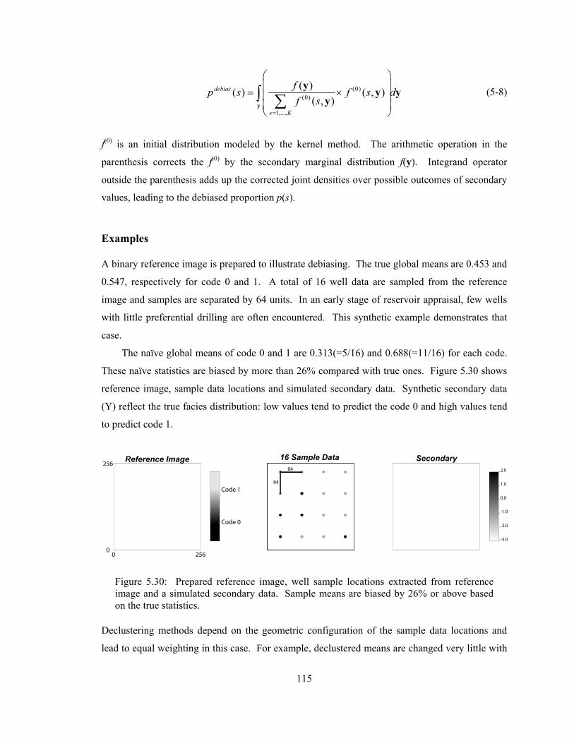
115

(0)(0)

1,...,

( )( ) ( , )( , )

debias

s K

fp s f s df s

=

⎛ ⎞⎜ ⎟= ×⎜ ⎟⎜ ⎟⎝ ⎠∫ ∑y

y y yy

(5-8)

f(0) is an initial distribution modeled by the kernel method. The arithmetic operation in the

parenthesis corrects the f(0) by the secondary marginal distribution f(y). Integrand operator

outside the parenthesis adds up the corrected joint densities over possible outcomes of secondary

values, leading to the debiased proportion p(s).

Examples

A binary reference image is prepared to illustrate debiasing. The true global means are 0.453 and

0.547, respectively for code 0 and 1. A total of 16 well data are sampled from the reference

image and samples are separated by 64 units. In an early stage of reservoir appraisal, few wells

with little preferential drilling are often encountered. This synthetic example demonstrates that

case.

The naïve global means of code 0 and 1 are 0.313(=5/16) and 0.688(=11/16) for each code.

These naïve statistics are biased by more than 26% compared with true ones. Figure 5.30 shows

reference image, sample data locations and simulated secondary data. Synthetic secondary data

(Y) reflect the true facies distribution: low values tend to predict the code 0 and high values tend

to predict code 1.

Figure 5.30: Prepared reference image, well sample locations extracted from reference image and a simulated secondary data. Sample means are biased by 26% or above based on the true statistics.

Declustering methods depend on the geometric configuration of the sample data locations and

lead to equal weighting in this case. For example, declustered means are changed very little with

Reference Image

Code 0

25600

256

64

64

Code 1

16 Sample Data Secondary

-3.0

-2.0

-1.0

0.0

1.0

2.0

116

respect to the change of cell sizes generating 0.325 and 0.675 as a declustered proportions which

are still biased by 23% based on the true values.

The initial bivariate distribution is modeled using kernel density estimation. Due to sample

data paucity, the modeled distribution curves appear very smooth. Figure 5.31 illustrates the

modeled f(s=0,y) and f(s=1,y) shown as a smooth solid line and the experimental data distribution

of Y shown as a bar chart.

Figure 5.31: Experimental data distribution and the modeled distribution f(s,y) based on sample data. The smooth line is a kernel estimator of bar chart.

The initial distributions are modified by a marginal constraint. The smooth curves shown in

Figure 5.31 are summed and compared with the secondary data distribution f(y). Figure 5.32

shows the modified distributions that have detailed variations in distribution. Those distributions

exactly reproduce the secondary data distribution as shown in the bottom of the figure. Debiased

global proportions of each code are obtained by (numerically) summing up the area below the

updated curves.

Collocated Secondary of Code 1

Secondary Value-3.00 -2.00 -1.00 0.00 1.00 2.00

0.000

0.050

0.100

0.150

0.200Collocated Secondary of Code 0

Number of Data 5mean -0.7

maximum 0.41minimum -1.99

Number of Data 11mean 0.37

maximum 1.92minimum -1.70

Secondary Value-3.00 -2.00 -1.00 0.00 1.00 2.00

0.000

0.050

0.100

0.150

0.200

117

Figure 5.32: The modified bivariate distributions by imposed marginal condition. A marginal distribution of secondary data is shown in the bottom.

The global proportions are summarized in the table below for comparison:

True 16 Samples with equal weights Cell declustering Debiasing

Code 0 0.453 0.313 0.325 0.415

Code 1 0.547 0.688 0.675 0.585

Cell declustering does not correct the bias because declustering techniques inherently assume the

sample data cover the full range of the data values, that is, declustering methods assume bias arise

only by spatial clustering, not by data value clustering. This example, however, shows that

collocated secondary data values are limited to [-1.99,0.41] and [-1.7,1.92] for code 0 and 1,

respectively (see summary statistics shown in Figure 5.31). The debiasing method is based on the

use of secondary data that are distributed over the full range of secondary values, say [-3.04,1.92]

for this example. The bias caused by clustering within the limited secondary values is mitigated

by the coverage of the secondary data.

Collocated Secondary of Code 1

Secondary Value-3.00 -2.00 -1.00 0.00 1.00 2.00

0.000

0.050

0.100

0.150

0.200Collocated Secondary of Code 0

Number of Data 5mean -0.7

maximum 0.41minimum -1.99

Number of Data 11mean 0.37

maximum 1.92minimum -1.70

Secondary Value-3.00 -2.00 -1.00 0.00 1.00 2.00

0.000

0.050

0.100

0.150

0.200

Secondary Value-3.00 -2.00 -1.00 0.00 1.00 2.00

0.000

0.040

0.080

0.120

Exhaustive Secondary DataNumber of Data 65536

mean 0.0maximum 1.92minimum -3.04

118

5.3 Integration of Soft Secondary and Geologic Map

Geologic map data are important to most reservoir studies. Geologic interpretation map is often

treated deterministically. Geostatistical reservoir models are then validated in light of a

conceptual geologic model. Geologic data is sometimes used for inferring the geostatistical

modeling parameters such as horizontal range, ratio of horizontal to vertical range in 3-D

variogram model and areal trend (Deutsch and Kupfersberger, 1999).

Whereas outcrop models can provide important information on reservoir architecture and

heterogeneity, it is not entirely clear how such information can be integrated while constructing a

probabilistic reservoir model (Caers and Zhang, 2004). Multipoint geostatistics is a newly

developed field for integrating the geologic patterns drawn from the outcrop models. This new

approach derives multiple point statistics from outcrop models, named as training images, and

then anchored them into well data (Journel and Alabert, 1989; Guardiano and Srivastava, 1993;

Strebelle, 2000). Soft secondary data are not directly integrated during the construction of local

probability distribution. To combine multiple-point statistics and secondary data, previous works

typically constructed local probability distribution conditioned to geologic data (or training

images), and conditioned to the soft secondary data, and then combine the calibrated probabilities

into the resulting probability. As described in Chapter 3, probability combination models have

been developed for this unifying individual probability.

In this section, the joint pdf modeling technique under marginal constraints is extended for

incorporating geologic data into soft secondary data. The main goal is to show that the proposed

method can integrate both continuous and discrete secondary data in a rigorous way, and to show

the improvements of integrating geologic map with soft secondary data. Soft secondary data

often fails to capture the local complex variation of the geologic feature because the soft

secondary data integration is pixel-based. A geology map that a prior geologic knowledge is

transferred into can reflect local complex features.

The joint relation between geologic map or image and soft secondary values is modeled with

a nonparametric method and the known marginal conditions are applied to modify the joint

distribution. By direct modeling of the joint distribution, the geologic information is fused into

the final probabilistic model without external data redundancy calibration that the probability

combination requires.

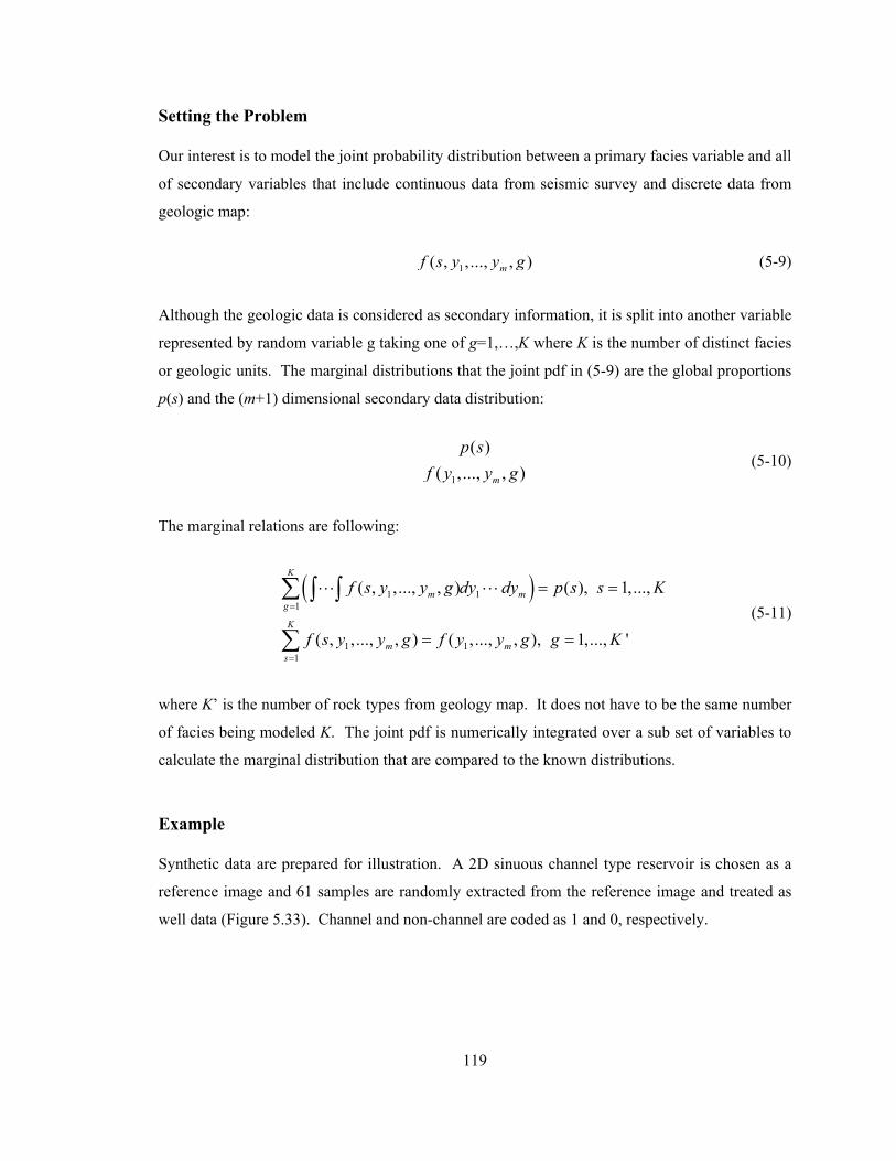
119

Setting the Problem

Our interest is to model the joint probability distribution between a primary facies variable and all

of secondary variables that include continuous data from seismic survey and discrete data from

geologic map:

1( , , ..., , )mf s y y g (5-9)

Although the geologic data is considered as secondary information, it is split into another variable

represented by random variable g taking one of g=1,…,K where K is the number of distinct facies

or geologic units. The marginal distributions that the joint pdf in (5-9) are the global proportions

p(s) and the (m+1) dimensional secondary data distribution:

1

( )( ,..., , )m

p sf y y g

(5-10)

The marginal relations are following:

( )1 1

1

1 11

( , ,..., , ) ( ), 1,...,

( , ,..., , ) ( ,..., , ), 1,..., '

K

m mg

K

m ms

f s y y g dy dy p s s K

f s y y g f y y g g K

=

=

⋅ ⋅ ⋅ ⋅ ⋅ ⋅ = =

= =

∑ ∫ ∫

∑ (5-11)

where K’ is the number of rock types from geology map. It does not have to be the same number

of facies being modeled K. The joint pdf is numerically integrated over a sub set of variables to

calculate the marginal distribution that are compared to the known distributions.

Example

Synthetic data are prepared for illustration. A 2D sinuous channel type reservoir is chosen as a

reference image and 61 samples are randomly extracted from the reference image and treated as

well data (Figure 5.33). Channel and non-channel are coded as 1 and 0, respectively.

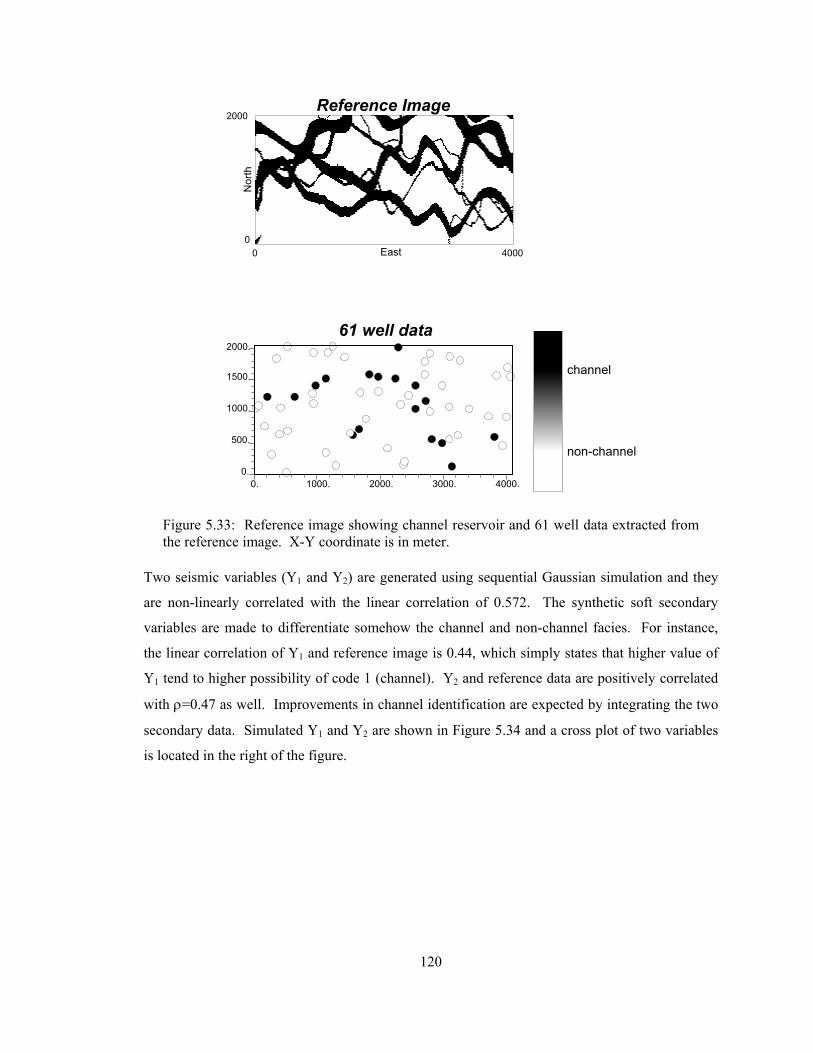
120

Figure 5.33: Reference image showing channel reservoir and 61 well data extracted from the reference image. X-Y coordinate is in meter.

Two seismic variables (Y1 and Y2) are generated using sequential Gaussian simulation and they

are non-linearly correlated with the linear correlation of 0.572. The synthetic soft secondary

variables are made to differentiate somehow the channel and non-channel facies. For instance,

the linear correlation of Y1 and reference image is 0.44, which simply states that higher value of

Y1 tend to higher possibility of code 1 (channel). Y2 and reference data are positively correlated

with ρ=0.47 as well. Improvements in channel identification are expected by integrating the two

secondary data. Simulated Y1 and Y2 are shown in Figure 5.34 and a cross plot of two variables

is located in the right of the figure.

Reference Image

EastN

orth

61 well data

0. 1000. 2000. 3000. 4000.

0 4000

0.

500.

1000.

1500.

2000.

2000

0

non-channel

channel

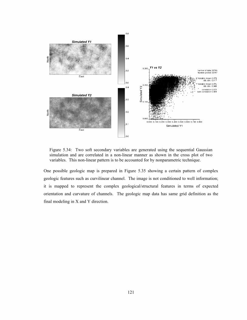
121

Figure 5.34: Two soft secondary variables are generated using the sequential Gaussian simulation and are correlated in a non-linear manner as shown in the cross plot of two variables. This non-linear pattern is to be accounted for by nonparametric technique.

One possible geologic map is prepared in Figure 5.35 showing a certain pattern of complex

geologic features such as curvilinear channel. The image is not conditioned to well information;

it is mapped to represent the complex geological/structural features in terms of expected

orientation and curvature of channels. The geologic map data has same grid definition as the

final modeling in X and Y direction.

122

Figure 5.35: A geologic map used for integrating with soft secondary data.

Due to the spatial clustering of well data, cell declustering was used for obtaining representative

global proportions which are to be used as one marginal constraint:

s=0 (non-channel) s=1(channel)

pnaive(s) 0.72 0.28

pdeclus(s) 0.669 0.339

The joint distribution of all secondary variables (soft secondary and geologic map) f(y1,y2,g) is

first modeled. The kernel density estimator was used to generate a smooth density distribution.

Since the geologic data is a type of discrete variable, the indicator function is added into the

product kernel estimator:

( )soft sec 2

,1 2

1 11 2

1( , , ) w InN

j j ii

i j j

y yf y y g g

Nh h h

=

= =

⎛ ⎞⎛ ⎞−= ×⎜ ⎟⎜ ⎟⎜ ⎟⎜ ⎟× ⎝ ⎠⎝ ⎠

∑ ∏ (5-12)

where N is the number of secondary values being equal to the number of modeling grids. I(gi) is

an indicator function of gi taking 1 if facies code gi of ith datum out of N corresponds to the facies

code g to be modeled, otherwise taking 0. The indicator function nullifies the kernel weights

when the facies code of modeling and the actual codes from the data are different. Figure 5.36

illustrates the modeled secondary data distributions f(y1,y2,g=0) and f(y1,y2,g=1). The range of y1

and y2 is discretized into 50 bins for numerical approximation. This level of discretization does

Geology

East

Nor

th

non-channel

channel

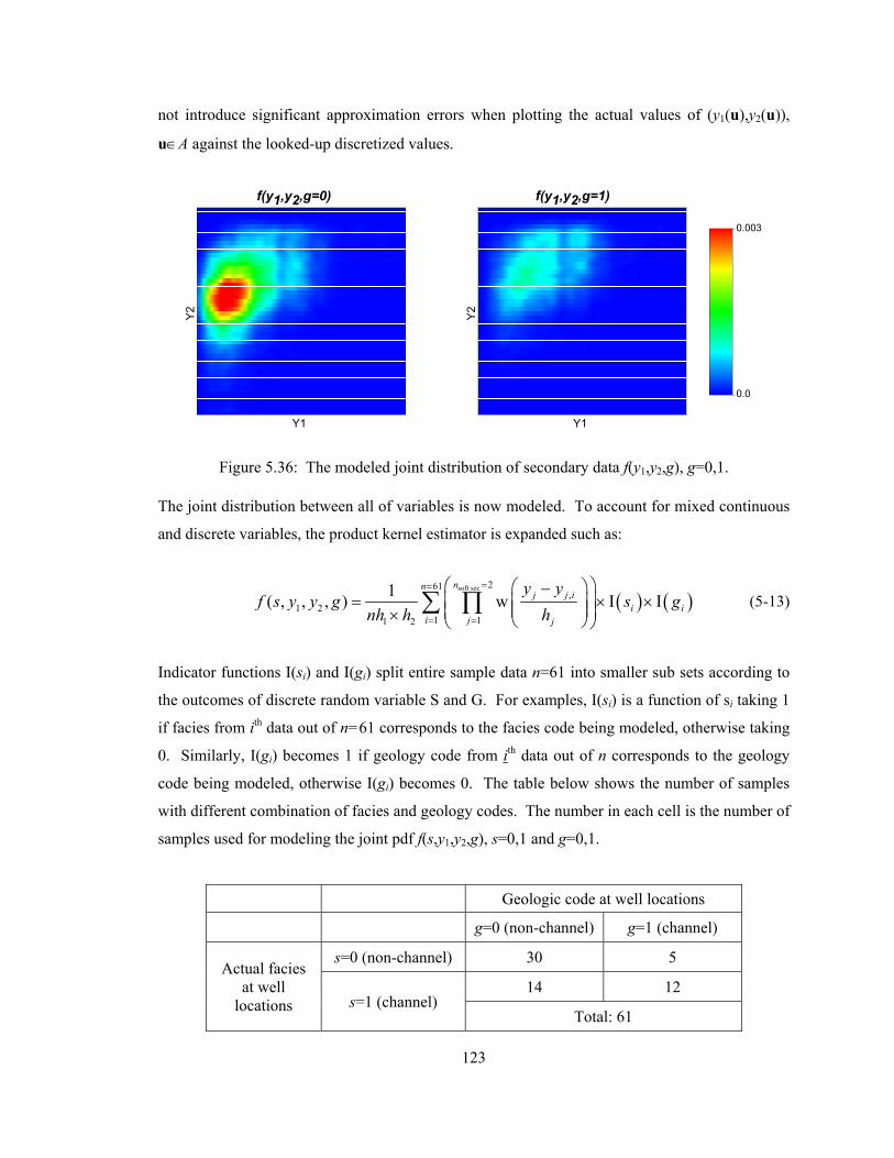
123

not introduce significant approximation errors when plotting the actual values of (y1(u),y2(u)),

u∈A against the looked-up discretized values.

Figure 5.36: The modeled joint distribution of secondary data f(y1,y2,g), g=0,1.

The joint distribution between all of variables is now modeled. To account for mixed continuous

and discrete variables, the product kernel estimator is expanded such as:

( ) ( )soft sec 261

,1 2

1 11 2

1( , , , ) w I Inn

j j ii i

i j j

y yf s y y g s g

nh h h

==

= =

⎛ ⎞⎛ ⎞−= × ×⎜ ⎟⎜ ⎟⎜ ⎟⎜ ⎟× ⎝ ⎠⎝ ⎠

∑ ∏ (5-13)

Indicator functions I(si) and I(gi) split entire sample data n=61 into smaller sub sets according to

the outcomes of discrete random variable S and G. For examples, I(si) is a function of si taking 1

if facies from ith data out of n=61 corresponds to the facies code being modeled, otherwise taking

0. Similarly, I(gi) becomes 1 if geology code from ith data out of n corresponds to the geology

code being modeled, otherwise I(gi) becomes 0. The table below shows the number of samples

with different combination of facies and geology codes. The number in each cell is the number of

samples used for modeling the joint pdf f(s,y1,y2,g), s=0,1 and g=0,1.

Geologic code at well locations

g=0 (non-channel) g=1 (channel)

Actual facies at well

locations

s=0 (non-channel) 30 5

s=1 (channel) 14 12

Total: 61

f(y1,y2,g=0) f(y1,y2,g=1)

Y1

Y2

Y1

Y2

0.0

0.003

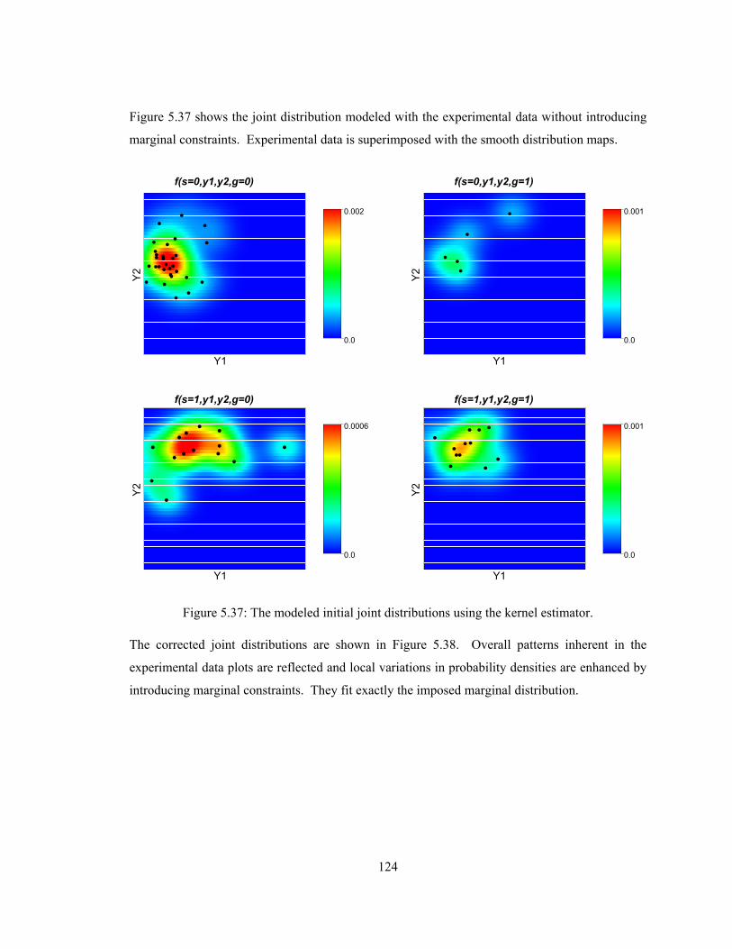
124

Figure 5.37 shows the joint distribution modeled with the experimental data without introducing

marginal constraints. Experimental data is superimposed with the smooth distribution maps.

Figure 5.37: The modeled initial joint distributions using the kernel estimator.

The corrected joint distributions are shown in Figure 5.38. Overall patterns inherent in the

experimental data plots are reflected and local variations in probability densities are enhanced by

introducing marginal constraints. They fit exactly the imposed marginal distribution.

f(s=0,y1,y2,g=0) f(s=0,y1,y2,g=1)

f(s=1,y1,y2,g=0) f(s=1,y1,y2,g=1)

0.0

0.002

0.0

0.001

0.0

0.0006

0.0

0.001

Y1

Y2

Y1

Y2

Y1

Y2

Y1

Y2

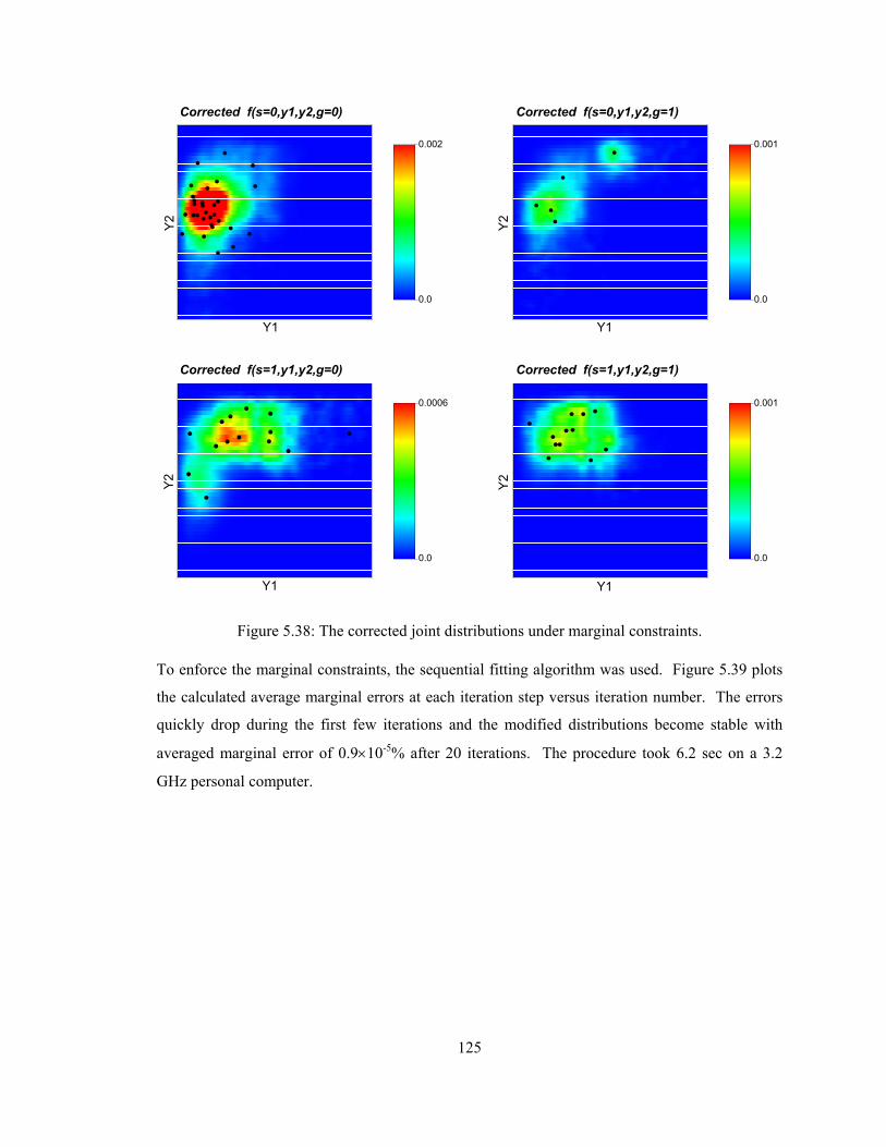
125

Figure 5.38: The corrected joint distributions under marginal constraints.

To enforce the marginal constraints, the sequential fitting algorithm was used. Figure 5.39 plots

the calculated average marginal errors at each iteration step versus iteration number. The errors

quickly drop during the first few iterations and the modified distributions become stable with

averaged marginal error of 0.9×10-5% after 20 iterations. The procedure took 6.2 sec on a 3.2

GHz personal computer.

Corrected f(s=0,y1,y2,g=0) Corrected f(s=0,y1,y2,g=1)

Corrected f(s=1,y1,y2,g=0) Corrected f(s=1,y1,y2,g=1)

0.0

0.002

0.0

0.001

0.0

0.0006

0.0

0.001

Y1

Y2

Y1

Y2

Y1

Y2

Y1

Y2

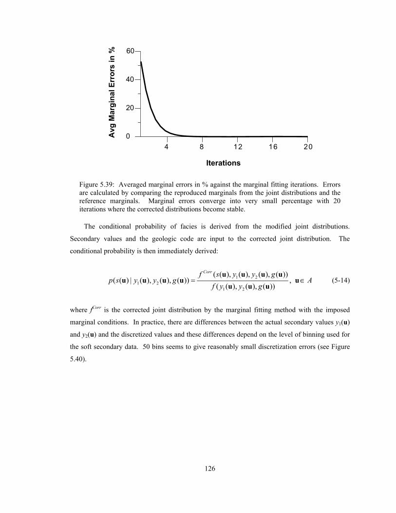
126

Figure 5.39: Averaged marginal errors in % against the marginal fitting iterations. Errors are calculated by comparing the reproduced marginals from the joint distributions and the reference marginals. Marginal errors converge into very small percentage with 20 iterations where the corrected distributions become stable.

The conditional probability of facies is derived from the modified joint distributions.

Secondary values and the geologic code are input to the corrected joint distribution. The

conditional probability is then immediately derived:

1 21 2

1 2

( ( ), ( ), ( ), ( ))( ( ) | ( ), ( ), ( )) ,

( ( ), ( ), ( ))

Corrf s y y gp s y y g A

f y y g= ∈

u u u uu u u u u

u u u (5-14)

where fCorr is the corrected joint distribution by the marginal fitting method with the imposed

marginal conditions. In practice, there are differences between the actual secondary values y1(u)

and y2(u) and the discretized values and these differences depend on the level of binning used for

the soft secondary data. 50 bins seems to give reasonably small discretization errors (see Figure

5.40).

4 8 12 16 200

20

40

60

Iterations

Avg

Mar

gina

l Err

ors

in %

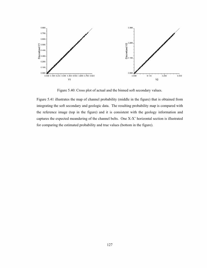
127

Figure 5.40: Cross plot of actual and the binned soft secondary values.

Figure 5.41 illustrates the map of channel probability (middle in the figure) that is obtained from

integrating the soft secondary and geologic data. The resulting probability map is compared with

the reference image (top in the figure) and it is consistent with the geology information and

captures the expected meandering of the channel belts. One X-X’ horizontal section is illustrated

for comparing the estimated probability and true values (bottom in the figure).

128

Figure 5.41: The estimated probability of channel is shown at the middle. A 1-D section through X-X’ is plotted in the bottom showing the true values either 0 (non-channel) or 1 (channel) and the secondary guided channel probability (grey line).

Prob of channel

East

X-X’

Nor

th

Reference Image

East

Nor

th

X X’

0.0

1.0

0 1000 2000 3000 4000

non-channel

channel

TrueEstimated prob oftrue

129

Figure 5.42 shows the probability of channel estimated from integrating soft secondary and

geology data (top), and from integrating soft secondary data only (bottom). Probabilities are

shown if pixels have 0.65 or higher probability of channel which is two times larger than the

global proportion of channel, p(channel) = 0.33. Channel connectivity is captured and complex

heterogeneity is accounted for which is a result of the input geologic information. The result

from considering soft secondary data shows a more patchy distribution of the channel probability.

Figure 5.42: The estimated probability of channel from integrating soft secondary and geology data, and soft secondary data only. Maps show the probability higher than 0.65: there is no special meaning of cutoff 0.65. This figure points out geologic heterogeneity is better reproduced and isolated pixels are reduced when considering both soft secondary and prior geologic information.

Prob of Channel > 0.65: soft sec + geology

East

Nor

th

Prob of Channel > 0.65: soft sec

East

Nor

th

0.

1.0

0.

1.0

130

5.4 Discussions

The main motivations for the method are that the joint distribution between the primary and the

secondary data is possible and the joint distribution of the secondary data is quite well-known.

The multivariate distribution modeling between the data is not enough. Marginal distribution

conditions are evaluated and the proposed marginal fitting algorithm corrects the modeled initial

joint distribution under the imposed conditions.

The multivariate distribution modeling under marginal constraints was applied to the various

secondary data integration examples: integrating continuous secondary data for facies modeling,

integrating large scaled soft secondary data for facies modeling and integrating soft secondary

and discrete geologic map for facies modeling. For these applications, data redundancy between

the secondary data is implicitly accounted for while the joint distribution modeling. The

examples showed that the marginal fitting algorithm is stable and fast: the averaged marginal

errors are quickly dropped and converged after a small number of iteration. The comparative

study from different integration techniques such as PCS versus multivariate modeling approach is

not done, but the reasonableness of the results are evaluated based on the fairness of the estimated

local probabilities and the reproduction of input statistics.

By enforcing the marginal distributions, the secondary derived probability result always

reproduced the declustered global proportion very well. The reproduced global proportions can

be far different without imposing marginal conditions.

The proposed multivariate modeling technique has been applied to the categorical variable

modeling. Application to the continuous variable modeling is described in Chapter 6. A new

interpretation of the Bayesian updating (BU) is demonstrated. It is shown that how the primary

data derived and the secondary data derived distributions can be integrated in a new form of BU

equation.

 

131

Chapter 6

Advanced Application of

the Multivariate

Distribution Modeling

6.1 Bayesian Updating

Bayesian updating (BU) technique was first proposed in 1996 by Doyen and since then the

technique has been widely adopted to integrate multiple soft secondary variables. BU is

fundamentally equivalent to collocated cokriging using the Markov type screening assumption

developed by Xu et al. but its formalism is different from the collocated cokriging (Doyen et al.,

1996; Chiles and Delfiner, 1999; Xu et al., 1992). Collocated cokriging is an extended form of

kriging expressed by a weighted linear combination of nearby primary and collocated secondary

data, and the technique expresses the updated distribution by the combination of probability

distributions conditioned to each primary and secondary variable. This section introduces the

detailed derivation of Bayesian updating equation and proposes an alternative form to the

conventional updating equation. The new expression gives an explicit interpretation of how

probability distributions derived from disparate data sources can be combined leading to the final

updated distribution, and where the global mean and variance intervene in the updating equation.

Because the new updating equation decomposes the influence of the primary and secondary

variable, separate calibration of secondary variable from primary variable is possible. An

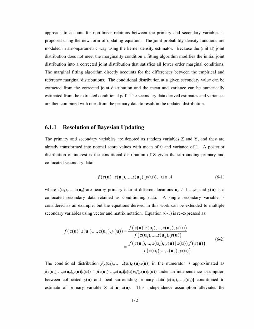
132

approach to account for non-linear relations between the primary and secondary variables is

proposed using the new form of updating equation. The joint probability density functions are

modeled in a nonparametric way using the kernel density estimator. Because the (initial) joint

distribution does not meet the marginality condition a fitting algorithm modifies the initial joint

distribution into a corrected joint distribution that satisfies all lower order marginal conditions.

The marginal fitting algorithm directly accounts for the differences between the empirical and

reference marginal distributions. The conditional distribution at a given secondary value can be

extracted from the corrected joint distribution and the mean and variance can be numerically

estimated from the extracted conditional pdf. The secondary data derived estimates and variances

are then combined with ones from the primary data to result in the updated distribution.

6.1.1 Resolution of Bayesian Updating

The primary and secondary variables are denoted as random variables Z and Y, and they are

already transformed into normal score values with mean of 0 and variance of 1. A posterior

distribution of interest is the conditional distribution of Z given the surrounding primary and

collocated secondary data:

  1( ( ) | ( ),..., ( ), ( )), nf z z z y A∈u u u u u   (6-1)

where z(u1),…, z(un) are nearby primary data at different locations ui, i=1,…,n, and y(u) is a

collocated secondary data retained as conditioning data. A single secondary variable is

considered as an example, but the equations derived in this work can be extended to multiple

secondary variables using vector and matrix notation. Equation (6-1) is re-expressed as:

 

( ) ( )( )

( ) ( )( )

11

1

1

1

( ), ( ),..., ( ), ( )( ) | ( ),..., ( ), ( )

( ),..., ( ), ( )

( ),..., ( ), ( ) | ( ) ( )( ),..., ( ), ( )

nn

n

n

n

f z z z yf z z z y

f z z y

f z z y z f zf z z y

=

=

u u u uu u u u

u u u

u u u u uu u u

  (6-2) 

The conditional distribution f(z(u1),…, z(un),y(u)|z(u)) in the numerator is approximated as

f(z(u1),…,z(un),y(u)|z(u)) ≅ f(z(u1),…,z(un)|z(u))×f(y(u)|z(u)) under an independence assumption

between collocated y(u) and local surrounding primary data [z(u1),…,z(un)] conditioned to

estimate of primary variable Z at u, z(u). This independence assumption alleviates the

133

requirement of inferring the joint distribution f(z(u1),…,z(un),y(u)|z(u)) which is difficult to model

because it requires joint modeling of mixed variables from different locations. Equation (6-2) is

approximated as:

  ( ) ( ) ( ) ( )( )

11

1

( ),..., ( ) | ( ) ( ) | ( ) ( )( ) | ( ),..., ( ), ( )

( ),..., ( ), ( )n

nn

f z z z f y z f zf z z z y

f z z y=

u u u u u uu u u u

u u u  (6-3) 

The conditional independence assumption decouples the posterior distribution into two terms: (1)

distribution associated with the primary data at different locations, f(z(u1),…,z(un)|z(u)), and (2)

the distribution associated with the primary and secondary variable relation, f(y(u)|z(u)). The

probabilistic terms in the right hand side of Equation (6-3) constitute a likelihood function that

treats the unknown estimate z(u) as fixed. They are re-expressed as probability functions of the

unknown estimate given the fixed data:

  ( ) ( )( )

( )( ) ( )1

1

( ) | ( ),..., ( ) ( ) | ( )( ) | ( ),..., ( ), ( ) ( )

( ) ( )n

n

f z z z f z yf z z z y f z C

f z f z= ⋅

u u u u uu u u u u

u u  (6-4) 

where normalizing C term is f(z(u1),…,z(un))×f(y(u))/(f(z(u1),…,z(un),y(u)). Although Bayesian

updating technique has been commonly used in many cases, there are few references explaining

how the final updating equations are reached (Neufeld and Deutsch, 2004; Deutsch and Zanon,

2004). Equation (6-4) provides a posterior distribution through the multiplication of three

probability distributions. f(z(u)|z(u1),…,z(un)) is a univariate conditional distribution of Z

conditioned to local nearby data z(u1),…,z(un). Under the multiGaussianity (MG) assumption,

kriging parametrically constructs the f(z(u)|z(u1),…,z(un)) as a Gaussian distribution with mean

equal to the kriging estimate and variance of kriging variance (Journel and Huijbregts, 1981;

Verly, 1983):

 2

1 22

1 ( ( ) ( ))( ( ) | ( ),..., ( )) exp2 ( )2 ( )

Pn

PP

z zf z z zσπσ

⎧ ⎫−= −⎨ ⎬

⎩ ⎭

u uu u uuu

  (6-5) 

where zP(u) and σ2P(u) are the estimate and estimation variance obtained by simple kriging at u.

Subscript P means that those are estimates from the primary data.

Under the linear relation assumption between the primary and secondary data the f(z(u)|y(u))

in Equation (6-5) becomes:

134

 2

22

1 ( ( ) ( ))( ( ) | ( )) exp22

S

SS

z zf z yσπσ

⎧ ⎫−= −⎨ ⎬

⎩ ⎭

u uu u   (6-6) 

zS(u) and σ2S(u) are the estimate and variance obtained by the relation between the primary and

secondary variables. Subscript S indicates they are secondary data derived moments. Due to the

linear relation assumption between Z and Y, the conditional mean and variance zS(u) and σ2S(u)

are simply calculated as zS(u) = ρ × y(u) and σ2S(u)=1–ρ2, where ρ is the linear correlation

coefficient between Z and Y. zS(u) depends on the local secondary value y(u) but the variance

σ2S(u) is constant over u∈A. The last term f(z(u)) in Equation (6-4) is a univariate Gaussian

distribution:

 2

22

1 ( ( ) )( ( )) exp22

z mf zσπσ

⎧ ⎫−= −⎨ ⎬

⎩ ⎭

uu   (6-7) 

Even though the primary variable Z has zero mean and unit variance (m=0, σ2=1), m and σ2

symbols are left in this equation. One can follow how the global mean and variance are used in

the final updating equation by letting the symbols remain.

Elementary probability distributions consisting of a posterior distribution are all Gaussian

(Equations (6-5), (6-6) and (6-7)). Multiplication of Gaussian distributions is another Gaussian;

thus, the posterior distribution is Gaussian as well. Equations shown in (6-5), (6-6) and (6-7) are

inserted into Equation (6-4) as follows:

 

( )( )

( )( )

( ) ( )

1

1

2

22 2

22 2

22

( ) | ( ),..., ( ), ( )

( ) | ( ),..., ( ) ( ) | ( )( )

( ) ( )

( ( ) ( ))1 exp2 ( )2 ( ) ( ( ) ( ))1 exp

2 ( )1 ( ( ) ) 2 ( )exp22

n

n

P

PP S

SS

f z z z y

f z z z f z yf z C

f z f z

z z

z z Cz m

σπσσπσ

σπσ

= ⋅

⎧ ⎫−−⎨ ⎬

⎧ ⎫⎩ ⎭ −= − ⋅⎨ ⎬

⎧ ⎫− ⎩ ⎭−⎨ ⎬⎩ ⎭

u u u u

u u u u uu

u u

u uuu u u

uu u

 (6-8) 

Terms inside the exponential functions are grouped and all terms independent of z(u) are

absorbed in the proportionality then:

135

  ( ) ( ) ( )1

2 2 2

2 2 2

( ( ) | ( ),..., ( ), ( ))

( ) ( ) ( ) ( ) ( )exp

2 ( ) 2 2 ( )

n

P S

P S

f z z z y

z z z m z zσ σ σ

∝

⎧ ⎫− − −⎪ ⎪− + −⎨ ⎬⎪ ⎪⎩ ⎭

u u u u

u u u u uu u

  (6-9) 

Equation (6-9) is arranged with respect to z(u):

 

1

22 2 2 2 2 2

( ( ) | ( ),..., ( ), ( ))

( )( )1 1 1exp ( ) ( )2 ( ) 2 2 ( ) ( ) ( )

n

SP

P S P S

f z z z y

zz mz z

BAσ σ σ σ σ σ

∝

⎧ ⎫⎪ ⎪⎡ ⎤ ⎡ ⎤⎪ ⎪− − + + + −⎨ ⎬⎢ ⎥ ⎢ ⎥

⎣ ⎦ ⎣ ⎦⎪ ⎪⎪ ⎪⎩ ⎭

u u u u

uuu uu u u u

 (6-10) 

Terms independent of z(u) are absorbed in the proportionality again. Equation (6-10) follows a

quadratic form of exp{-Az2 + Bz} where A and B are parameterized coefficients. This can be

easily converted into the basic form of Gaussian function:

  { } ( )( )

1

22

( ( ) | ( ),..., ( ), ( ))

( ) / 2exp ( ) ( ) exp

2 1/ 2

nf z z z y

z B AAz Bz

A

∝

⎧ ⎫−⎪ ⎪− + ∝ −⎨ ⎬⎪ ⎪⎩ ⎭

u u u u

uu u

  (6-11) 

The posterior distribution f(z(u)|z(u1),…,z(un),y(u)) becomes a Gaussian distribution with the

mean of B/2A and variance of 1/2A while A and B are defined in Equation (6-10):

  2 1( ) and ( )2 2BU BU

BzA A

σ = =u u   (6-12) 

where zBU(u) and 2 ( )BUσ u are the mean and variance of the posterior distribution. The Bayesian

updated variance and estimate at location u are finally:

 

2 2 2 2

2 2 2 2

1 1 1 1( ) ( ) ( )

( ) ( )( )( ) ( ) ( )

BU P S

BU SP

BU P S

z zz m

σ σ σ σ

σ σ σ σ

= + −

= + −

u u u

u uuu u u

  (6-13) 

136

A set of Equation (6-13) is a new form of Bayesian updating that can be compared with the

conventional form below:

 

2 2

2 2 2 2

2 22

2 2 2 2

( ) ( ) ( )( )( ) ( ) ( ) ( )

( ) ( )( )( ) ( ) ( ) ( )

P S S PBU

P P S S

P SBU

P P S S

z zz σ σσ σ σ σ

σ σσσ σ σ σ

+=

− +

=− +

u u uuu u u u

u uuu u u u

  (6-14) 

The equations in (6-13) and (6-14) are exactly same when m = 0 and σ2 = 1 in Equation (6-13).

The main advantage of the new expression is that the updated parameters zBU and σ2BU are clearly

decomposed into combination of local and global parameters derived from diverse sources. One

possible applications of the new form would be accounting for the non-stationarity in the global

statistics such as m(u) and σ(u) instead of m(u)=m and σ(u)=σ (Hong and Deutsch, 2008).  

6.1.2 Accounting for Non-linear Relations between Primary and Secondary Variables

Several assumptions have been made to derive the Bayesian updating equation and the key

assumptions are: (1) multiGaussianity of primary variables at different locations, which allows

constructing the local conditional distribution f(z(u)|z(u1),…,z(un)) by simple kriging at u, and (2)

a linear relation between primary and secondary variables, which allows building the conditional

distribution f(z(u)|y(u)) by the linear correlation coefficient ρ. Only under this Gaussian

assumption on the distributions (multivariate Gaussian in spatial context and multivariate

Gaussian in variable context) is the analytical derivation of updating is possible.

Relaxing the linear relation assumption between primary and secondary variables is

considered here. The multiGaussianity assumption is still adopted to build the local conditional

distribution f(z(u)|z(u1),…,z(un)). Conventional Bayesian updating assumes the Gaussian relation

after univariate normal score transformation of each variable. An illustration shown in Figure 6.1

represents a highly non-linear feature between two normal scored variables (normal scored values

of porosity and permeability from the Amoco data set). Gaussianity of univariate marginal

distribution is a necessary condition, but not a sufficient condition for joint Gaussianity.

 

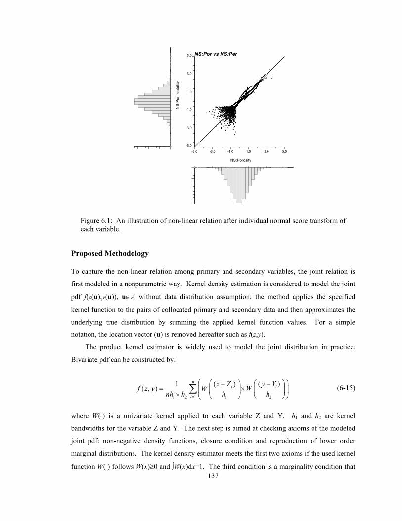
137

Figure 6.1: An illustration of non-linear relation after individual normal score transform of each variable. 

Proposed Methodology

To capture the non-linear relation among primary and secondary variables, the joint relation is

first modeled in a nonparametric way. Kernel density estimation is considered to model the joint

pdf f(z(u),y(u)), u∈A without data distribution assumption; the method applies the specified

kernel function to the pairs of collocated primary and secondary data and then approximates the

underlying true distribution by summing the applied kernel function values. For a simple

notation, the location vector (u) is removed hereafter such as f(z,y).

The product kernel estimator is widely used to model the joint distribution in practice.

Bivariate pdf can be constructed by:

 11 2 1 2

1 ( ) ( )( , )n

i i

i

z Z y Yf z y W Wnh h h h=

⎛ ⎞⎛ ⎞ ⎛ ⎞− −= ×⎜ ⎟⎜ ⎟ ⎜ ⎟× ⎝ ⎠ ⎝ ⎠⎝ ⎠

∑   (6-15) 

where W(⋅) is a univariate kernel applied to each variable Z and Y. h1 and h2 are kernel

bandwidths for the variable Z and Y. The next step is aimed at checking axioms of the modeled

joint pdf: non-negative density functions, closure condition and reproduction of lower order

marginal distributions. The kernel density estimator meets the first two axioms if the used kernel

function W(⋅) follows W(x)≥0 and ∫W(x)dx=1. The third condition is a marginality condition that

NS

:Per

mea

bilit

y

NS:Por vs NS:Per

-5.0 -3.0 -1.0 1.0 3.0 5.0

-5.0

-3.0

-1.0

1.0

3.0

5.0

NS:Porosity

138

the p-variate joint pdf should reproduce p′-variate pdf where p′ < p. The following are the

marginal conditions that the modeled bivariate pdf must meet:

  ( , ) ( ),f z y dz f y y= ∀∫   (6-16) 

  ( , ) ( ),f z y dy f z z= ∀∫   (6-17) 

The marginal relation described in Equation (6-16) states that integration of the joint probability

distribution over possible outcomes of the primary data should amount to the distribution of the

secondary variable Y, f(y). The second marginal relation (6-17) states that integration of the joint

probability distribution over possible outcomes of the secondary variable should reproduce the

distribution of the primary variable Z, f(z). The global distribution of the primary variable f(z) is

experimentally obtained from well samples. The secondary data pdf f(y) is modeled with the

densely sampled values over the area and the abundance of samples makes a very reliable f(y).

Given the marginal relations, the marginal fitting algorithm is used to impose them on the joint

pdf f(z,y). The marginals are derived from initial joint distribution and they are compared with

the reference marginals. The differences are directly corrected in the correcting procedure. This

correcting process consists of the following steps:

Step1. Model the distribution of secondary variable, f(y) and global distribution of primary

variable, f(z). Declustering is considered for obtaining an unbiased f(z) if required.

Step2. Model the joint distribution f(z,y) and define it as f(0) to differentiate from the

resulting joint distribution.

Step3. Scale the f(0) to ensure the marginal distribution shown in Equation (6-16). The

scaling equation below is proposed for ensuring the imposed marginal condition:

  (0) (1)(0)

( )( , ) ( , )( , )

f yf z y f z yf z y dz

× →∫

  (6-18) 

The ratio f(y)/∫f(z,y)dz is a modifying factor. If the marginal relation (6-16) is satisfied

then this factor becomes 1 leading to no change in f(0). Otherwise, f(0) is adjusted by the

modifying factor that accounts for the differences between the reference f(y) and

reproduced marginal distribution ∫f(0)(z,y)dz. The corrected distribution under the marginal

condition is set as f(1) for the next step.

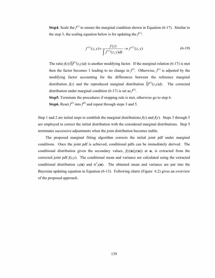
139

Step4. Scale the f(1) to ensure the marginal condition shown in Equation (6-17). Similar to

the step 3, the scaling equation below is for updating the f(1):

  (1) (2)(1)

( )( , ) ( , )( , )f zf z y f z y

f z y dy× →∫

  (6-19) 

The ratio f(z)/∫∫f(1)(z,y)dy is another modifying factor. If the marginal relation (6-17) is met

then the factor becomes 1 leading to no change in f(1). Otherwise, f(1) is adjusted by the

modifying factor accounting for the differences between the reference marginal

distribution f(z) and the reproduced marginal distribution ∫∫f(1)(z,y)dy. The corrected

distribution under marginal condition (6-17) is set as f(2).

Step5. Terminate the procedures if stopping rule is met, otherwise go to step 6.

Step6. Reset f(2) into f(0) and repeat through steps 3 and 5.

Step 1 and 2 are initial steps to establish the marginal distributions f(z) and f(y). Steps 3 through 5

are employed to correct the initial distribution with the considered marginal distributions. Step 5

terminates successive adjustments when the joint distribution becomes stable.  

The proposed marginal fitting algorithm corrects the initial joint pdf under marginal

conditions. Once the joint pdf is achieved, conditional pdfs can be immediately derived. The

conditional distribution given the secondary values, f(z(u)|y(u)) at u, is extracted from the

corrected joint pdf f(z,y). The conditional mean and variance are calculated using the extracted

conditional distribution zS(u) and σ2S(u). The obtained mean and variance are put into the

Bayesian updating equation in Equation (6-13). Following charts (Figure 6.2) gives an overview

of the proposed approach.

140

Figure 6.2: Workflow for the proposed approach

The suggested algorithm accounts for non-linear features between primary and secondary

variables and its modeled joint pdf exactly reproduces lower order marginal distributions. The

conditional distribution given any value of secondary data can be drawn from the obtained joint

distribution. The extracted conditional distribution may not be univariate Gaussian; it can be any

shape (see the extracted univariate conditional pdf at step 3 in the above flow chart). Univariate

Gaussian fitting is used for the extracted conditional distribution because the conditional pdf

z

y

f(z,y)

corr

f (z,y)corr

z

yy(u)

f(z(u)|y(u))

1. Model the f(z,y) by kernel density estimation

2. Correct the initial f(z,y) with marginal conditions (Sequential marginal fitting algorithm) and set as f (z,y)

3. Extrac the conditional distribution f(z|y) from f (z,y) given secondary values

4. Calculate the mean and variance of the extracted f(z(u)|y(u))

5. Set the calculated mean and variance as zS(u) and σ2S(u) and inert them into the updating equation

f (z,y)corr

z

ycorr

collocated samples

141

f(z(u)|y(u)) can be integrated with the primary-variable based conditional pdf f(z(u)|z(u1),…,z(un))

to an updated Gaussian distribution when the constituent distributions are both Gaussian.  

6.1.3 Examples

The 2D Amoco data set is used for the application of the more flexible Bayesian updating method.

Permeability is considered as the primary variable to be modeled and porosity is considered as the

secondary variable. Sampled porosities at 62 wells are simulated to initialize the exhaustive

secondary data. 65-by-65 grids nodes are defined in X and Y directions. Figure 6.3 illustrates the

simulated porosity field and the permeability samples at well locations. Figure 6.4 shows a

scatter plot of the normal scored permeability and porosity. The bivariate relation is not Gaussian

despite both marginals being univariate normal. Evaluating the bivariate Gaussianity can be

performed through plotting the squared generalized distances from data pairs against the chi-

square distances (Johnson and Wichern, 2002). An illustration shown in the right of Figure 6.4 is

a plot for the calculated distances from normal scored data pairs and analytical chi-square

distances (Johnson and Wichern, 2002). The plot should resemble the straight line through the

origin if bivariate normality is guaranteed. Systematic curved pattern shown on the chi-square

distance plot suggests a lack of Gaussianity for the normal scored data pairs.

Figure 6.3: Simulated porosity used as secondary variable (left) for predicting permeability and sampled permeability at 62 well locations (right).

Simulated Porosity (used as sec var)

East

Nor

th

0 10400 ft 0 10400 ft0

10400 ft

-2.0

0.0

2.0

Locations of 62 wells

-2.0

0.0

2.0NS:perm

0

10400 ft

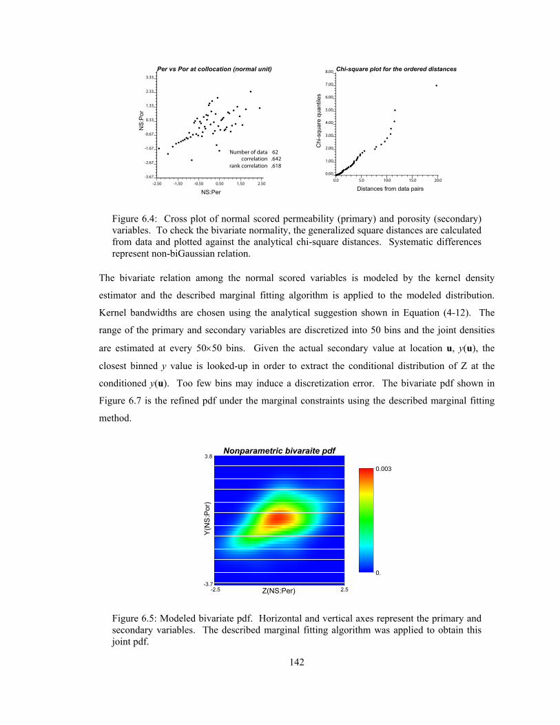
142

Figure 6.4: Cross plot of normal scored permeability (primary) and porosity (secondary) variables. To check the bivariate normality, the generalized square distances are calculated from data and plotted against the analytical chi-square distances. Systematic differences represent non-biGaussian relation.

The bivariate relation among the normal scored variables is modeled by the kernel density

estimator and the described marginal fitting algorithm is applied to the modeled distribution.

Kernel bandwidths are chosen using the analytical suggestion shown in Equation (4-12). The

range of the primary and secondary variables are discretized into 50 bins and the joint densities

are estimated at every 50×50 bins. Given the actual secondary value at location u, y(u), the

closest binned y value is looked-up in order to extract the conditional distribution of Z at the

conditioned y(u). Too few bins may induce a discretization error. The bivariate pdf shown in

Figure 6.7 is the refined pdf under the marginal constraints using the described marginal fitting

method.

Figure 6.5: Modeled bivariate pdf. Horizontal and vertical axes represent the primary and secondary variables. The described marginal fitting algorithm was applied to obtain this joint pdf.

NS

:Por

NS:Per

Per vs Por at collocation (normal unit)

-2.50 -1.50 -0.50 0.50 1.50 2.50

-3.67

-2.67

-1.67

-0.67

0.33

1.33

2.33

3.33

Number of data 62correlation .642

rank correlation .618

Chi

-squ

are

quan

tiles

Distances from data pairs

Chi-square plot for the ordered distances

0.0 5.0 10.0 15.0 20.00.00

1.00

2.00

3.00

4.00

5.00

6.00

7.00

8.00

Nonparametric bivaraite pdf

0.

0.003

Y(N

S:P

or)

Z(NS:Per)

3.8

-2.5 2.5-3.7

143

The averaged marginal errors quickly drop during first few iteration steps. 100 marginal fitting

iterations make the bivariate pdf stable and it took a few seconds on a 3 GHz personal computer.

Based on the resulting bivariate distribution, the conditional means and variances are

calculated. In this nonparametric modeling, the conditional mean and variance are not

determined by the coefficient of correlation but are calculated based on the extracted conditional

distribution f(z(u)|y(u)), u∈A. The conditional mean is numerically calculated through the binned

values zk, k=1,…,50:

 50 50

1 1

( , ( ))( ) { ( ) | ( )} ( | ( ))( ( ))k

L k k kk k

f z ym E Z Y y z f z y zf y= =

= = = =∑ ∑ uu u u uu

  (6-20) 

The extracted 1-D pdf curve f(zk,y(u)) is a function of the binned primary variable zk for a fixed

y(u). The conditional pdf f(zk|y(u)) is acquired by dividing f(zk,y(u)) by f(y(u)). The conditional

variances are calculated by:

 [ ] [ ]

2

50 502 2

1 1

( ) { ( ) | ( )}( , ( ))( ) ( | ( )) ( )

( ( ))

L

kk L k k L

k k

Var Z Y yf z yz m f z y z m

f y

σ

= =

= =

= − = −∑ ∑

u u uuu u u

u

  (6-21) 

Where mL(u) is a conditional mean of Z given the y(u). Figure 6.6 demonstrates the conditional

means and variances given the secondary data value (NS:por). Black dots superimposed with the

bivariate pdf map represent the calculated conditional means. The conditional variances are

plotted in the right. The conditional means are not linear and the conditional variances are not

constant during the range of the secondary variable. Moreover, they are related to the variation of

secondary values. For example, the change of conditional variance is rapid when the given

secondary values (NS:por) are high or very low. In the intermediate range of secondary data,

about from -2.1 to 1.8, the conditional variance tends to decrease with a moderate slope. Figure

6.7 shows the estimates and estimation variance derived from the secondary data.

144

Figure 6.6: Conditional means and variances obtained from the joint pdf modeled in a nonparametric way. Black dots (left) are the calculated conditional means of NS:per with respect to the varying secondary values NS:por. Open circles (right) are the conditional variances with respect to the secondary values.

Figure 6.7: Secondary data derived estimates and variances

The conventional BU approach assumes a linear relation between the primary and secondary

variable so that it provides a constant estimation variance over the domain. Figure 6.8 shows the

comparison of the conditional estimates and estimation variance from the Gaussian assumption

and the nonparametric approach. A correlation of 0.642 is calculated from the data pairs of

normal scored porosity and permeability as plotted by open circles in the figure. The black solid

line is an estimate given the secondary data with the linear regression, and grey dashed line is an

estimate from the nonparametric approach. The regression line overestimates the permeability

when the conditioned secondary value is high or low. The estimates from the two different

approaches are similar when the intermediate range of secondary values is given. The right figure

of Figure 6-8 represents the estimation variances given the secondary values. The variances

0.003

0.0

-2.50 -1.50 -0.50 0.50 1.50 2.50

-3.68

-2.68

-1.68

-0.68

0.32

1.32

2.32

3.32

-3.68

-2.68

-1.68

-0.68

0.32

1.32

2.32

3.32

densities

NS:perm Conditional variance

NS

:por

NS

:por

conditional mean of NS:perm conditional variance of NS:perm

0.2 0.3 0.4 0.5 0.6 0.7 0.8 0.9 1.0

Estimate from Secondary Data

-1.0

0.0

1.0

Estimation Variance from Secondary Data

0.0

1.0

East

Nor

th

0 10400 ft0

10400 ft

East

Nor

th

0 10400 ft0

10400 ft

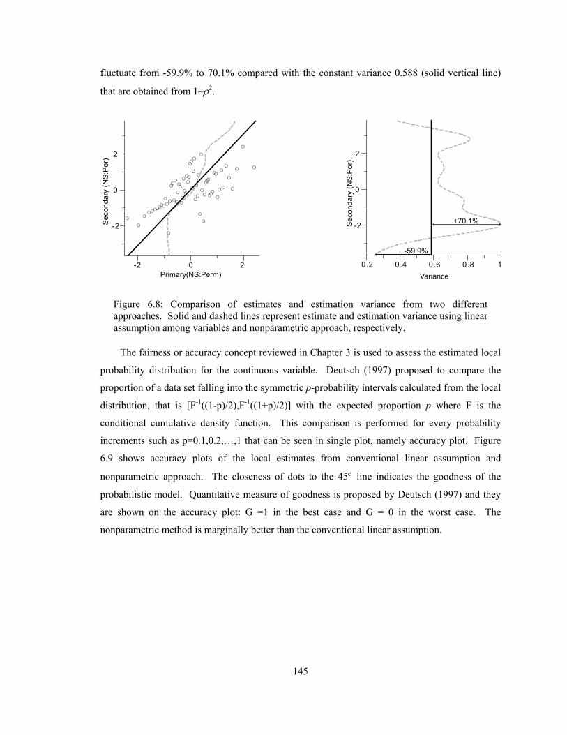
145

fluctuate from -59.9% to 70.1% compared with the constant variance 0.588 (solid vertical line)

that are obtained from 1–ρ2.

Figure 6.8: Comparison of estimates and estimation variance from two different approaches. Solid and dashed lines represent estimate and estimation variance using linear assumption among variables and nonparametric approach, respectively.

The fairness or accuracy concept reviewed in Chapter 3 is used to assess the estimated local

probability distribution for the continuous variable. Deutsch (1997) proposed to compare the

proportion of a data set falling into the symmetric p-probability intervals calculated from the local

distribution, that is [F-1((1-p)/2),F-1((1+p)/2)] with the expected proportion p where F is the

conditional cumulative density function. This comparison is performed for every probability

increments such as p=0.1,0.2,…,1 that can be seen in single plot, namely accuracy plot. Figure

6.9 shows accuracy plots of the local estimates from conventional linear assumption and

nonparametric approach. The closeness of dots to the 45° line indicates the goodness of the

probabilistic model. Quantitative measure of goodness is proposed by Deutsch (1997) and they

are shown on the accuracy plot: G =1 in the best case and G = 0 in the worst case. The

nonparametric method is marginally better than the conventional linear assumption.

-2 0 2

-2

0

2

Primary(NS:Perm)

Sec

onda

ry (N

S:P

or)

0 .2 0.4 0.6 0.8 1

-2

0

2

Sec

onda

ry (N

S:P

or)

Variance

+70.1%

-59.9%

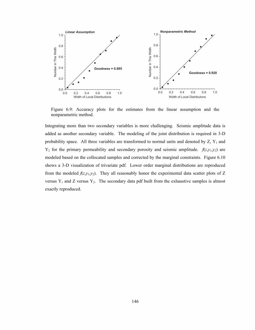
146

Figure 6.9: Accuracy plots for the estimates from the linear assumption and the nonparametric method.

Integrating more than two secondary variables is more challenging. Seismic amplitude data is

added as another secondary variable. The modeling of the joint distribution is required in 3-D

probability space. All three variables are transformed to normal units and denoted by Z, Y1 and

Y2 for the primary permeability and secondary porosity and seismic amplitude. f(z,y1,y2) are

modeled based on the collocated samples and corrected by the marginal constraints. Figure 6.10

shows a 3-D visualization of trivariate pdf. Lower order marginal distributions are reproduced

from the modeled f(z,y1,y2). They all reasonably honor the experimental data scatter plots of Z

versus Y1 and Z versus Y2. The secondary data pdf built from the exhaustive samples is almost

exactly reproduced.

Num

ber i

n Th

is W

idth

Width of Local Distributions

Linear Assumption

Goodness = 0.885

0.0 0.2 0.4 0.6 0.8 1.00.0

0.2

0.4

0.6

0.8

1.0

Goodness = 0.920

Num

ber i

n Th

is W

idth

Width of Local Distributons

Nonparametric Method

0.0 0.2 0.4 0.6 0.8 1.00.0

0.2

0.4

0.6

0.8

1.0

147

Figure 6.10: A trivariate pdf modeled by kernel density estimator with marginal correction process: the primary and two secondary variables are denoted as Z, Y1 and Y2, respectively. The lower order bivariate pdf reproduced from the trivariate pdf are checked with the input data scatter plots and distribution.

Figure 6.11 illustrates the estimates and estimation variances with respect to the conditioned

secondary data Y1 and Y2. Upper row in the figure shows the estimates and the estimation

variance from the linear assumption and the bottom row shows the estimates and estimation

variance from the nonparametric approach. The estimates change in overall from low to high

when the conditioned Y1 and Y2 change from low to high values because of positive correlation

among variables. The effect of nonparametric approach is more obvious in the estimation

variance as shown at the lower right in Figure 6.11. The linear assumption results in a constant

estimation variance regardless of the conditioned secondary values Y1 and Y2. The

nonparametric method generates the estimation variance that varies depending on the given

secondary data values. The estimate and estimation variance over all locations u∈A are shown in

Figure 6.12. The corresponding accuracy plot is shown in Figure 6.13 compared with the

0.0001

0.0

Z Y1

Y2

f(z,y1,y2)

Reproduced f(y1,y2)

f(z,y1)

f(z,y2)

Modeled f(y1,y2) fromexhaustive samples

3.5

3.67-3.67-3.5

3.5

3.67-3.67-3.5

3.67

3.67-3.67-3.67

3.67

3.67-3.67-3.67

collocated samples of z and y1

collocated samples of z and y2

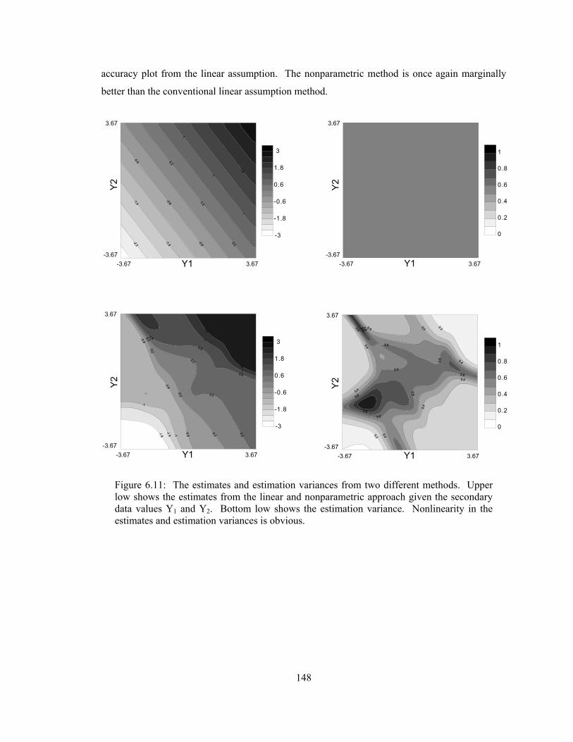
148

accuracy plot from the linear assumption. The nonparametric method is once again marginally

better than the conventional linear assumption method.

Figure 6.11: The estimates and estimation variances from two different methods. Upper low shows the estimates from the linear and nonparametric approach given the secondary data values Y1 and Y2. Bottom low shows the estimation variance. Nonlinearity in the estimates and estimation variances is obvious.

-3

-1.8

-0.6

0.6

1.8

3

-3

-1.8

-0.6

0.6

1.8

3

-3.67-3.67

3.67

3.67

-3.67-3.67

3.67

3.67

-3.67-3.67

3.67

3.67

-3.67-3.67

3.67

3.67

0

0.2

0.4

0.6

0.8

1

0

0.2

0.4

0.6

0.8

1

Y2

Y1

Y2

Y1

Y2

Y1

Y2

Y1

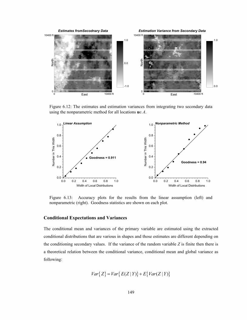
149

Figure 6.12: The estimates and estimation variances from integrating two secondary data using the nonparametric method for all locations u∈A. 

Figure 6.13: Accuracy plots for the results from the linear assumption (left) and nonparametric (right). Goodness statistics are shown on each plot.

Conditional Expectations and Variances

The conditional mean and variances of the primary variable are estimated using the extracted

conditional distributions that are various in shapes and those estimates are different depending on

the conditioning secondary values. If the variance of the random variable Z is finite then there is

a theoretical relation between the conditional variance, conditional mean and global variance as

following:

{ } { } { }( | ) ( | )Var Z Var E Z Y E Var Z Y= +

Estimates fromSecodnary Data

-1.0

0.0

1.0

Estimation Variance from Secondary Data

0.0

1.0

East

Nor

th

0 10400 ft0

10400 ft

East

Nor

th

0 10400 ft0

10400 ft

Goodness = 0.911

Num

ber i

n Th

is W

idth

Width of Local Distributions

Linear Assumption

0.0 0.2 0.4 0.6 0.8 1.00.0

0.2

0.4

0.6

0.8

1.0

Goodness = 0.94

Num

ber i

n Th

is W

idth

Width of Local Distributions

Nonparametric Method

0.0 0.2 0.4 0.6 0.8 1.00.0

0.2

0.4

0.6

0.8

1.0

150

which is known as the law of total variance stating that the total variability of the primary

variable is sum of the variance of the conditional means and the average of the conditional

variances (Billingsley, 1995). Another relation, known as the law of total expectation, is

{ } { }( | )E Z E E Z Y=

These equations could be a way for evaluating the appropriateness of the modeled joint

distribution because these theoretical relations are violated if the joint distribution is not a licit

distribution.

6.2 Discussions

Bayesian updating has been widely adopted to integrate secondary data. The updating equation;

however, is difficult to understand how information source is combined. New interpretation of

Bayesian updating equation is introduced. Although the conventional and new expressions are

mathematically equivalent, new forms have some advantages rather than old ones. New form of

updating equation decomposes the posteriori pdf into the combination of elementary pdf related

to the primary and secondary data and it can be clearly understood how different information

source is combined.

The multivariate distribution modeling method is applied to account for the non-linear

features among the primary and the secondary variables. Joint pdf is modeled in a nonparametric

way and sequential marginal fitting algorithm refines the modeled joint pdf into the corrected

joint pdf that meets all marginal constraints. The described marginal fitting algorithm directly

accounts for the differences between empirical and reference marginal distributions. Given the

joint pdf, the conditional pdf at a secondary value is extracted, and estimate and estimation

variances are calculated using the extracted conditional pdf. The resulting estimation variance;

thus, is not constant but locally varying which better reflects the relation of the primary and

secondary variables.

The results are evaluated based on the described accuracy criteria and compared with the

parametric method. In this particular example, the nonparametric method is marginally better

than the parametric method.

151

Chapter 7

Summary and Conclusions

Inevitably, numerical reservoir models are uncertain because direct measurements are available at

relatively few well locations relative to the size of the whole modeling area. With the limited

amount of well data, large uncertainty exists in the spatial distribution of the primary variables

being modeled. Supplementary information such as multiple seismic attributes and conceptual

geologic data can aid in predicting the primary variables more accurately and realistically.

Incorporating all available data, however, is not an easy task because data are different

measurements, exhibit nonlinear features, different precision and redundancy. For the problem of

integrating diverse data, some previous studies adapted a Gaussian assumption so that the

multivariate distribution of the given data is assumed multivariate Gaussian after univariate

transformation. This type of parametric model is simple and easy to apply at the cost of not

accounting for complex multivariate relations. Other previous studies are based on the

combination of the univariate conditional probabilities that are calibrated individually. The

essential part of such probability combination methods is to properly quantify the redundancy

between the secondary data. Incorrectly quantified redundancy parameter makes the results

biased leading to unfairly very high or low probabilities as demonstrated in Chapter 3. A new

redundancy parameter calibration method is studied in Chapter 3 named as the Lamda model.

The model calibrates the redundancy parameters from the differences between the known and the

estimated values. Although the new model outperforms other combination models, the relation

between data redundancy and the calibrated weights is not clearly understood.

The later part of the thesis, that is a key contribution of this work, is about the multivariate

analysis framework to integrate available diverse data. The motivation for the developed

152

technique is that one can model the joint relation among the secondary data very reliably, and

directly model the joint relation among the primary and the secondary data.

The methodology consists of two main parts. The first part is to model the multivariate

distribution nonparametrically so that the complex multivariate features are reproduced.

Nonparametric method allows the joint modeling of a mixture of continuous and discrete

variables. By directly modeling the joint relations, data redundancy is directly accounted for. No

explicit calibration is required. In reservoir modeling studies, the use of nonparametric density

modeling is not new. Recent studies applied nonparametric techniques to integrate seismic data

for the reservoir attribute modeling (Saggaf et al., 2000; Doyen, 2007). The work in this

dissertation advanced the multivariate distribution modeling further. The second part of the

developed multivariate analysis framework is to impose the known marginal distribution

constraints. The modeled multivariate distribution is refined under the lower order distributions

composed of the primary and the secondary data. The proposed iteration algorithm evaluates the

marginal conditions and corrects the multivariate distribution. The correction procedure is done

sequentially with respect to each of the primary and the secondary data distributions. The

algorithm is proved to be converged to the correct distribution in Chapter 4 and is shown to be

practically fast through particular examples in Chapter 5. The iteration is terminated when the

stopping condition is met. Since the algorithm modifies the given joint distribution alternately

using the marginals of the primary and the secondary, the averaged marginal error calculated at

each iteration is used as a stopping rule. The first few iterations dropped the errors quickly.

Finally, the obtained multivariate distribution accounts for the complex joint relations, data

redundancy and meets all axioms of probability distribution functions.

As demonstrated in section 4.2, the marginal fitting procedure begins with the initial joint

distribution that is modeled based on the collocated samples of primary and secondary data.

Under few collocated samples which can happen to generate the wrong initial distribution, the

resulting joint distribution after marginal fitting step will be far different from the underlying true

distribution even it satisfies all of the necessary marginal conditions. This inconsistency case

cannot be overcome by the proposed method.

Chapter 5 and 6 of this dissertation demonstrated several applications of the proposed

methodology including integration of continuous secondary data for categorical variable

modeling, integrating a mixture of continuous and categorical secondary data for categorical

variable modeling, and integration of continuous secondary data for continuous variable modeling.

The examples demonstrated that the proposed methodology is an effective method to integrate

diverse data without distribution assumption and ad-hoc redundancy calibration.

153

Comparative study with other existing techniques was not performed. However, the results

were evaluated based on the internal checking criteria and they all met the criteria satisfactorily.

Although the multivariate approach is robust and theoretically sound, the probability

combination methods would be appealing in some applications. They are suitable for 3D trend

modeling by combining lower order 1D vertical and 2D areal trends (Deutsch, 2002). Another

application of the probability combining approach would be the case of non-isotopic sampling of

the secondary data. An underlying assumption of the multivariate modeling approach is that all

secondary variables are isotopically sampled over the entire domain of study. If different data

have different spatial coverage, then the modeling of the joint relation and correcting of the

multivariate distribution under marginal constraints may not be reliable. The probability

combination approach may be more useful for that case.

Ideas for Future Work

Although the essential ideas of the new method are developed in this dissertation, several issues

still remain. The following are some avenues for future research.

Nonparametric Modeling Methods

There are many nonparametric distribution modeling techniques available. Some techniques

outperform the kernel method comprehensively implemented in this work. For example, the

standard kernel density estimator is not an appropriate technique when applied to long-tailed or

bounded distributions. The standard kernel estimator uses a fixed kernel bandwidth that may

result in oversmoothing in areas of sparse samples and undersmoothing in the areas of abundant

samples. An adaptive kernel method varies the kernel bandwidth locally based on the scarcity of

samples used for the density modeling; kernel bandwidths increase with few samples and

decrease with many samples.

Another nonparametric modeling technique is to use copular functions. Copula functions are

joint distributions defined on the space of cumulative probabilities [0,1]. The copula approach

transforms the samples of variables into the unit interval [0,1] and models the joint relation in [0,1]

by analytically pre-defined copula functions. Because samples are uniquely mapped into the unit

interval [0,1] and the joint relation is described in the unit space, binning of the variables is not

required. Kernel density estimation requires binning the data. This procedure becomes

computationally heavy if the number of bins is large with many variables. The copula method,

154

however, is a bin-free nonparametric modeling technique. Besides, some functions are

parametrically defined to describe the joint relations. The possible drawback of the method

would be a strong reliance of the joint distribution on the uniform marginal distribution. By

keeping the marginal distribution uniform, the separability of possible outcomes of the primary

variable is not possible in the joint distribution.

Variable Aggregation

The kernel density estimation is a heavy solution in terms of CPU and memory resources. The

computational cost largely depends on the number of variables being integrated. For example,

density estimation should be done at every Bm where B is the number of bins and m is the number

of secondary data. In practice, the number of secondary data, m would be limited to 5 by

ignoring irrelevant variables, merging highly relevant variables or both ignoring and merging.

Data aggregation could be a pre-processing step before the multivariate analysis. In statistics, the

principal component or factor analysis are widely used dimension reduction techniques. Super

secondary variable concept based on the collocated cokriging merges the relevant variables by

accounting for the redundancy among secondary variables and the closeness to the primary

variable. No matter what aggregation methods are used, the purpose of variable aggregation is to

reduce the number of secondary variables with the least loss of information in the original

variables.

155

Bibliography

Almeida, A.S. and Journel, A.G. (1994) Joint simulation of multiple variables with a Markov-type coregionalization model. Mathematical Geology, 26:565-588. Ballin, P.R., Journel, A.G. and Aziz, K.A. (1992) Prediction of uncertainty in reservoir performance forecasting. Journal of Canadian Petroleum Technology, 31:52-62. Billingsley, P. (1995) Probability and measure: Wiley-Interscience. Benediktsson, J.A. and Swain, P.H. (1992) Consensus theoretic classification methods. IEEE Transactions on Systems, Man and Cybernetics, 22:688-704. Bishop, Y.M.M, Fienberg, S.E. and Holland, P.W. (1977) Discrete multivariate analysis. MIT Press Bordley, R.F. (1982) A multiplicative formula for aggregating probability assessments. Management Science, 28:1137-1148. Bourgault, G (1994) Robustness of Noise Filtering by Kriging Analysis. Mathematical Geology,26:733-752. Bressan, M. and Vitria, J. (2003) Nonparametric discriminant analysis and nearest neighbor classification. Pattern Recognition Letters, 24:2743-2749. Cacoullos, T. (1966) Estimation of a multivariate density. Annals of the Institute of Statistical Mathematics, 18:178-189. Castro, S. (2005) A probabilistic approach to jointly integrate 3D/4D seismic, production data and geological information for building reservoir models. PhD thesis, Stanford University, Stanford, CA. Castro, S., Caers, J., Otterlei, C., H∅ye, T., Andersen, T. and Gomel, P. (2005) A probabilistic integration of well log, geological information, 3D/4D seismic and production data: application to the Oseberg field, SPE 103152. Carr, J.R. (1990) Application of Spatial Filter Theory to Kriging. Mathematical Geology, 22:1063-1079. Caers, J. and Ma, X. (2002) Modeling conditional distributions of facies from seismic using neural nets. Mathematical Geology, 34:143-167.

156

Caers, J. and Zhang, T. (2004) Multiple-point geostatistics: A quantitative vehicle for integrating geologic analogues into multiple reservoir models. In Integration of outcrop and modern analogues in reservoir modeling: AAPG Memoir 80:383-394. Chiles, J-P, Delfiner, P. (1999) Geostatistics Modeling Spatial Uncertainty, John Wiley & Sons. Clemen, R.T. and Winkler, R.L. (1999) Combining probability distributions from experts in risk analysis. Risk Analysis, 19:187-203. Coleou, T. (2002) Time-lapse filtering and improved repeatability with automatic factorial co-kriging (AFACK). Paper A-18, presented at the 64th EAGE Conference and Exhibition, Florence, 27–30 May. Datta-Gupta, A., Lake, L.W. and Pope, G.A. (1995) Characterizing heterogeneous permeable media with spatial statistics and tracer data using sequential simulated annealing. Mathematical Geology, 27:763-787. de Matos, M.C., Osorio, P.L.M. and Johann, P.R.S. (2007) Unsupervised seismic facies analysis using wavelet transform and self-organizing maps. Geophysics, 72:9-21. Deming, W.E. and Stephan, F.F. (1940) On a least squares adjustment of a sampled frequency table when the expected marginal totals are known. Annals of Mathematical Statistics, 11:427-444. Deutsch, C.V. (1996) Direct assessment of local accuracy and precisioin, Geostatistics Wollongong 1996, edited by Baafi, E., Kluwer Academic Publihsers. Deutsch, C.V. and Journel, A.G. (1998) GSLIB: Geostatistical Software Library and User’s Guide. Oxford University Press, New York. Deutsch, C.V. (2002) Geostatistical Reservoir Modeling. Oxford University Press, New York. Deutsch. C.V. (1999) A Short note on cross validation of facies simulation methods. In Report 1, Centre for Computational Geostatistics, Edmonton, AB, Canada. Deutsch, C.V. (1992) Annealing techniques applied to reservoir modeling and the integration of geological and engineering(well test) data. PhD thesis, Stanford University, Stanford, CA. Deutsch, C.V. and Hewett, T.A. (1996) Challenges in reservoir forecasting. Mathematical Geology, 28:829-842. Deutsch, C.V., Srinivasan, S. and Mo, Y. (1996) Geostatistical reservoir modeling accounting for precision and scale of seismic data. SPE 36497. Deutsch, C.V. (1996) Constrained smoothing of histograms and scatterplots with simulated annealing, Technometrics, 38:266-274.

157

Deutsch, C.V. and Zanon, S.D. (2004) Direct prediction of reservoir performance with Bayesian updating under a multivariate Gaussian model, Paper presented at the Petroleum Society’s 5th Canadian International Petroleum Conference, Calgary, Alberta. Doyen, P.M. (2007) Seismic Reservoir Characterization An Earth Modeling Perspective, EAGE Publications, Houten, Netherlands. Doyen, P.M., den Boer, L.D. and Pillet, W.R. (1996) Seismic porosity mapping in the Ekofisk field using a new form of collocated cokriging. SPE 36498. Dowd, P.A., Pardo-Iguzquiza, E. (2005) Estimating the boundary surface between geologic formations from 3D seismic data using neural networks and Geostatistics. Geophysics,70: P1-P11. Dumay, J. and Fournier, F. (1988) Multivariate statistical analyses applied to seismic facies recognition. Geophysics, 53: 1151-1159. Fournier, F. and Derain J-F (1995) A statistical methodology for deriving reservoir properties from seismic data. Geophysics, 60:1437-1450. Friedman, N., Geiger, D. and Goldszmidt, M. (1997) Bayesian network classifiers. Machine Learning, 29:131-163. Galli, A, Gerdil-Neuillet, F, Dadou, C (1983) Factorial kriging analysis: a substitute to spectral analysis of magnetic data. In Geostatistics for Natural Resource Characterization, edited by Verly, G., David, M., Journel, A.G. and Marechal, A., Riedel Publishers, Dordrecht. Gomez-Hernandez, J. (1997) Issues on environmental risk assessment. Geostatistics Wollongong 1996, edited by Baafi, E.Y., Kluwer Academic Publishers. Goovaerts, P. (1992) Factorial kriging analysis: a useful tool for exploring the structure of multivariate spatial soil information. Journal of Soil Science,43:597-619. Goovaerts, P (1997) Geostatistical for Natural Resources Evaluation. Oxford University Press, New York. Goovaerts, P. (1997) Geostatistics for natural resources evaluation. Oxford University press, New York. Guardiano, F.B. and Srivastava, R.M. (1993) Multivariate geostatistics: beyond bivariate moments. Geostatistics Troia 1992, edited by Soares, A. Hall, P., Sheather, S.J., Joines, M.C. and Marron, J.S. (1991) On optimal data-based bandwidth selection in kernel density estimation. Biometrika, 78:263-269. Haldorsen, H.H. and Damsleth, E. (1990), Stochastic modeling. Journal of Canadian Petroleum Technology, 42:404-412. Harris, J.M. and Langan, R.T. (1997) Crosswell seismic fills the gap in Geophysical Corner. AAPG Explorer, January.

158

Hong, S. and Deutsch, C.V. (2008) A short note: an alternative interpretation of Bayesian updating for non-stationary modeling, In Report 10, Centre for Computational Geostatistics, Edmonton, AB, Canada. Hoffman, B. T., Wen, X-H, Strebelle, S., and Caers, J. (2005) Geologically consistent history matching of a deepwater turbidite reservoir, SPE 95557. Isaaks, E.H. and Srivastava, R.M. (1989) Introduction to Applied Geostatistics. Oxford University Press, New York, USA. Ireland, C.T. and Kullback, S. (1968) Contingency tables with given marginals, Biometrika, 55:179-188. Izenman, A.J. (1991) Recent developments in nonparametric density estimation. Journal of the American Statistical Association, 86:205-224. Jaquet, O (1989) Factorial Kriging Analysis Applied to Geological Data from Petroleum Exploration. Mathematical Geology,21: 683-691. Journel, A.G. (1999) Markov models for cross-covariances. Mathematical Geology, 31:955-964. Journel, A.G. and Alabert, F. (1989) Non-Gaussian data expansion in the earth sciences. Terra Nova, 1:123-134. Journel, A.G. and Huijbregts, Ch.J. (1978) Mining Geostatistics. Academic Press, London. Journel, A.G. (2002) Combining knowledge from diverse sources: an alternative to traditional data independence hypotheses. Mathematical Geology, 34:573-596. John, A.K., Lake, L.W., Torres-Verdin, C. and Srinivasa, S. (2008) Seismic facies identification and classification using simple statistics. SPE Reservoir Evaluation & Engineering, 11:984-990. Johnson, R.A. and Wichern, D.W. (2002) Applied to Multivariate Statistical Analysis. Prentice Hall, New Jersey. Krzanowski, W.J. (1993) The location model for mixtures of categorical and continuous variables. Journal of Classification, 10:25-49. Krishnan, S. (2008) The tau model for data redundancy and information combination in earth sciences: theory and application. Mathematical Geosciences, 40:705-727. Krishnan, S. (2004) Combining diverse and partially redundant information in the earth sciences. PhD dissertation, Stanford University, Stanford, CA. Krishnan, S., Boucher, A. and Journel, A.G. (2005) Evaluating information redundancy through the tau model. Geostatistics Banff 2004, edited by Leuangthong and Deutsch, Springer, Dordrecht, Netherlands, 1037-1046. Kullback, S. and Leibler, R.A. (1951) On information and sufficiency, Annals of Mathematical Statistics, 22:79-86.

159

Kupfersberger, H, Deutsch, C.V. and Journel, A.G. (1998) Deriving constraints on small-scale variograms due to variograms of large-scale data. Mathematical Geology, 30:837-852. Li, Q. and Racine, J. (2003) Nonparametric estimation of distributions with categorical and continuous data. Journal of Multivariate Analysis, 86:266-292. Lee, T., Richards, J.A. and Swain, P.H. (1987) Probabilistic end evidential approaches for multisource data analysis. IEEE Transactions on Geosciences and Remote Sensing, GE-25:283-293 Liu, Y., Harding, A., Gilbert, R. and Journel, A.G. (2004) A work flow for multiple-point geostatistical simulation. Geostatistics Banff 2004. edited by Leuangthong, O. and Deutsch, C.V., Springer, Dordrecht, Netherlands, 245-254. Lumley, D.E., Behrens, R.A., and Wang, Z. (1997) Assessing the technical risk of a 4-D seismic project. The Leading Edge, 16:1287-1291. Marron, J.S. (1987) A comparison of cross –validation techniques in density estimation. Annals of Statistics, 15:152-162. Mukerji, T., Jorstad, A., Avseth, P., Mavko, G. and Granli, J.R. (2001a) Mapping lithofacies and pore-fluid probabilities in a North Sea reservoir: seismic inversions and statistical rock physics. Geophysics, 66:988-1001. Neufeld, C. and Deutsch, C.V. (2004) Incorporating secondary data in the prediction of reservoir properties using Bayesian updating. In Report 6, Centre for Computational Geostatistics, Edmonton, AB, Canada. Nelson, R.B. (2006) An introduction to copulas. New York, Springer. Parzen, E. (1962) On the estimation of a probability density function and the mode. Annals of Mathematical Statistics, 33:1065-1076. Park, B.U. and Marron, J.S. (1990) Comparison of data-driven bandwidth selectors. Journal of the American Statistical Association, 85:66-72. Pearl, J. (1988) Probabilistic reasoning in intelligent systems: networks of plausible inference (representation and reasoning). Morgan Kaufmann Publisher, San Francisco. Polyakova, E.I. and Journel, A.G. (2007) The nu expression for probabilistic data integration. Mathematical Geology, 39:715-733. Pyrcz, M.J., Gringarten, E., Frykman, P. and Deutsch, C.V. (2006) Representative input parameters for geostatistical simulation. edited by Coburn, T.C., Yarus, R.J. and Chambers, R.L., Stochastic Modeling and Geostatistics: Principles, Methods and Case Studies, Vol. II: 123-137. Rosenblatt, M. (1956) Remarks on some nonparametric estimates of a density function. Annals of Mathematical Statistics, 27:832-837.

160

Roberts, S.J. (1996) Parametric and non-parametric unsupervised cluster analysis, Pattern Recognition,30:261-272. Saggaf, M.M. and Robinson, E.A. (2003) Estimation of reservoir properties from seismic data by smooth neural networks. Geophysics, 68:1969-1983. Saggaf ,M.M., Toksoz, M.N. and Marhoon, M.I. (2003) Seismic facies classification and identification by competitive neural networks. Geophysics, 68:1984-1999. Scott, D.W. (1992) Multivariate Density Estimation: Theory, Practice, and Visualization. John Wiley and Sons, Inc., New York. Silverman, B.W. (1986) Density Estimation for Statistics and Data Analysis, Chapman and Hall, London. Srivastava, R.M. (1987) Minimum variance or maximum profitability?, CIM Bulletin, 80:63-68. Stain, S.R., Baggerly, K.A. and Scott, D.W. (1994) Cross-validation of multivariate densities. Journal of the American Statistical Association, 89:807-817. Strebelle, S. (2002) Conditional simulation of complex geological structures using multi-point statistics. Mathematical Geology, 34:1-21. Verly, G. (1983) The Multigaussian approach and its applications to the estimation of local reserves. Mathematical Geology, 15:259-286. Wackernagel, H. (2003) Multivariate Geostatistics. Springer, Berlin. Wand, M.P. and Jones, M.C. (1993) Comparison of smoothing parameterizations in bivariate kernel density estimation. Journal of the American Statistical Association, 88:520-528. Wen, X.H., Deutsch, C.V., Cullick, A.S. (2002) Construction of Geostatistical aquifer models integrating dynamic flow and tracer data using inverse technique. Journal of Hydrology, 255:151-168. Winkler, R.L. (1981) Combining probability distributions from dependent information sources. Management Science, 27:479-488. Xu,W., Tran, T.T., Srivastava, R.M. and Journel, A.G. (1992) Integrating seismic data in reservoir modeling: the collocated cokriging alternative. SPE 24742, Washington, DC, October 4-7, 1992. Yao, T, Mukerji, T, Journel, A.G., Mavko, G. (1999) Scale Matching with Factorial Kriging for Improved Porosity Estimation from Seismic Data. Mathematical Geology,31: 23-46.

161

A Symbols and Selected Terms

A The area of modeling

B Number of bins for the nonparametric modeling

BU Bayesian updating

CI Conditional independence

(D1,...,Dm) Generic notation for m secondary data

E-type The expected values calculated from the multiple realizations

FK Factorial kriging

f(s,y) Joint distribution of the primary variable s and soft secondary variable y

f(0) The modeled joint distribution without marginal correction

f(k) The modeled joint distribution with marginal correction at kth iteration step

γ(h) Variogram of distance h

hi Kernel bandwidth for the variable i

i**(u;s) Indicator estimate using the primary and secondary data at u\

KDE Kernel density estimation

K The number of facies

MDE Multivariate density estimation

MISE Mean integrated square errors

n Number of well samples

OFK Ordinary factorial kriging

PCS Probability combination schemes

p(s) Global proportion of categorical variable s=1,…,K

psec Secondary data derived probability

PR Permanence of Ratios

pCI The conditional probability from the CI model

pPR The conditional probability from the PR model

pLamda 1 The conditional probability from the Lamda model with calibration method 1

pLamda 2 The conditional probability from the Lamda model with calibration method 2

162

pTau The conditional probability from the Tau model

s Random variable representing discrete facies

SFK Simple factorial kriging

SISIM Sequential Indicator Simulation

SGSIM Sequential Gaussian Simulation

SMF Sequential Marginal Fitting

NTG Net-to-gross

W(⋅) Univariate kernel function

(y1,…,ym) Continuous secondary variable

Zs(u), σs(u) Estimate and estimation variance of the primary variable derived from the

secondary data at u

Zp(u), σp(u) Estimate and estimation variance of the primary variable derived from the

primary data at u

163

Appendix A

Factorial Kriging for Reservoir

Feature Identification and Extraction

Kriging aims to estimate a regionalized variable at an unsampled location (Journel and Huijbregts,

1978; Deutsch and Journel, 1998). To apply the kriging algorithm the spatial structures should be

modeled with the variogram or covariance. When dealing with nested variogram or covariance

structures it may be of interest to extract specific structures such as isotropic short range feature,

anisotropic long range feature or nugget effect. Such filtering that excludes undesired features

and enhances interesting features can be achieved by factorial kriging (Carr, 1990; Goovaerts,

1997; Deutsch and Journel, 1998). The number of sub-features and the magnitude of that features

are chosen from the modeled nested variogram. The effectiveness of factorial kriging in filtering

undesired features and in enhancing target features has been discussed in previous works.

Goovaerts (1992) applied factorial kriging into the analysis of multivariate spatial soil data.

Noise filtering inherent in exploration geologic data and its robustness irrespective of additive or

multiplicative noise type are discussed in Bourgault (1994). Application of factorial kriging to

well data and seismic data is investigated in Jaquet (1989), Tao et al. (1999), and Dowd and

Pardo-Iguzquiza (2005). Coleou (2002) presented the applicability of factorial cokriging to 4-D

seismic data. Coleou (2002) showed that common spatial features between seismic surveys

acquired at time t0 and t1 can be extracted by cross variogram modeling of those seismic data.

Previous works discussed above demonstrated powerful capability of factorial kriging to

decompose spatial features according to the scale and filter out the random noise.

A case study will show how factorial kriging is applied to identify and enhance target

features. Conventional factorial kriging is considered first based on ordinary kriging that

amounts to locally estimate the mean of Z(u) within each search; the mean of each factor is

assumed to be zero. Each factor is extracted using ordinary factorial kriging and the results are

164

discussed. Some drawbacks of the method are observed. Simple kriging concept is applied to the

conventional factorial kriging, which is called simple factorial kriging in this appendix. We

observed the significant difference from conventional ordinary factorial kriging. Factorial kriging

has smoothing effect so as simple kriging. Simple factorial kriging was also applied to filter the

noise inherent in many secondary datasets. The nugget effect due to measurement errors can be

removed. Factorial kriging can filter out any unwanted structure that has been included in the

variogram model.

Another application of factorial kriging is to integrate only relevant features extracted from

original data. In some cases, the large scale features are more important than local variability. In

this case, large scale features are extracted from secondary data using factorial kriging, then

cokriging is used to estimate the primary variable with hard data and the large scale factor. The

applicability of the method is tested using synthetic and real data and the results are discussed.

A.1 Linear Model of Regionalization

Factorial kriging analysis is a geostatistical method relying on the assumption that a regionalized

phenomenon can be seen as a linear sum of varied independent sub-phenomena playing at

different scales and each sub-phenomena presents its own spatial feature captured on variogram

or covariance model. These linearly summed variogram or covariance comprise the variogram or

covariance of the regionalized phenomenon.

The choice of a variogram model and its fitting must be validated by geologic and

geophysical understanding of the phenomenon under study such as directions of anisotropy,

measurement errors or artifacts, and the number of nested structure. From the experimental

variogram of a regionalized variable, these key parameters are fitted to build a permissible

variogram model that captures the spatial features of the attribute under study and adding

geologic background knowledge may lead to a more robust model.

Factorial kriging analysis allows different components corresponding to these spatial features

(also called factors hence the name factorial kriging) to be estimated. If factors act at different

scales and they are apparent in the variogram model, then these factors can be decomposed by

factorial kriging.

Figure A.1 shows the spatial components at different scales and their corresponding

variograms: nugget, small scale isotropic and large scale anisotropic factors are simulated. By the

linear model of regionalization, each factors are summed to make the primary attribute that is of

interest by traditional kriging. The goal of factorial kriging is to decompose the primary attribute

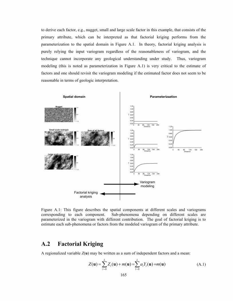
165

to derive each factor, e.g., nugget, small and large scale factor in this example, that consists of the

primary attribute, which can be interpreted as that factorial kriging performs from the

parameterization to the spatial domain in Figure A.1. In theory, factorial kriging analysis is

purely relying the input variogram regardless of the reasonableness of variogram, and the

technique cannot incorporate any geological understanding under study. Thus, variogram

modeling (this is noted as parameterization in Figure A.1) is very critical to the estimate of

factors and one should revisit the variogram modeling if the estimated factor does not seem to be

reasonable in terms of geologic interpretation.

Figure A.1: This figure describes the spatial components at different scales and variograms corresponding to each component. Sub-phenomena depending on different scales are parameterized in the variogram with different contribution. The goal of factorial kriging is to estimate each sub-phenomena or factors from the modeled variogram of the primary attribute.

A.2 Factorial Kriging

A regionalized variable Z(u) may be written as a sum of independent factors and a mean:

0 0

( ) ( ) ( ) ( ) ( )L L

l l ll l

Z Z m a Y m= =

= + = +∑ ∑u u u u u (A.1)

Nugget

Small scale isotropic

-1.0

0.0

1.0

-2.0

0.0

2.0

-1.0

0.0

1.0

-1.0

0.0

1.0Large scale anisotropic

Sum of all factors

0

γ

0.00

0.20

0.40

0.60

0.80

1.00

1.20

γ

Distance0 40 80 120 160 200

Distance0 40 80 120 160 200

Distance0 40 80 120 160 200

Distance0 40 80 120 160 200

0.00

0.20

0.40

0.60

0.80

1.00

1.20

γ

0.00

0.20

0.40

0.60

0.80

1.00

1.20

γ

0.00

0.20

0.40

0.60

0.80

1.00

1.20

Spatial domain Parameterizaztion

Factorial kriginganalysis

Variogrammodeling

166

The (L+1) standard factors Zl(u) = alYl(u) all have a mean of 0 and a variance of 1. The al

parameters are stationary, that is, they do not depend on location. The mean and variance of the

Z(u) variable are given by:

0 0

{ ( )} ( ) ( ) { ( )} ( ) ( )L L

l l l ll l

E Z E a Y m a E Y m m= =

⎧ ⎫= + = + =⎨ ⎬

⎩ ⎭∑ ∑u u u u u u (A.2)

2 2

0 0

{ ( )} { ( )} 0L L

l l ll l

Var Z a Var Y a= =

= + =∑ ∑u u (A.3)

The variance of Z(u) follows such a simple expression because m(u) is a constant and the Y(u)

factors are standard and independent. These characteristics of m and Y also lead to a

straightforward expression for the variogram of the Z(u) variable:

( ) ( )2

0

L

l ll

aγ γ=

= ∑h h (A.4)

The Z(u) regionalized variable is fully specified by m(u), the (L+1) al values, and the L+1

variograms γl(h). The 2la parameters are the magnitude of each nested structure. One has access

to the original data values Z(u) at sample locations and the modeled variogram. One does not

directly sample the la parameters that specify the importance of each factor. Moreover, the

measurements of the Yl(u) factors are not available. The factors are distinguishable only when

the constituent variograms γl(h) are different from one another. The reasonableness of factorial

kriging depends entirely on the fitted nested structures.

A.2.1 Ordinary Factorial Kriging (OFK)

Assume that the variable Z(u) consists of factors Zl(u) and locally unknown mean values m(u).

Consider the problem of estimating the spatial component Zl(u) of the decomposition. The OK

estimator of the spatial component is:

*,

1

( ) ( ), 0,...,n

l lZ Z l Lα αα

λ=

= =∑u u (A.5)

*,

1

( ) ( )n

mm Zα αα

λ=

= ∑u u (A.6)

The weights are location dependent, but the (u) has been dropped for clear notation. ,lαλ and

,mαλ are the weights for the estimation of l and mean factor. It is noted that *( )lZ u is an l factor

167

estimate using original data Z(uα), which contains (L+1) factors, but unknown and only the

weights are different being associated with l factor. The constraints on the weights are

established to ensure the unbiasedness:

,1

1n

mαα

λ=

=∑ and ,1

0n

lαα

λ=

=∑ (A.7)

*, ,

1 1

since, { ( ) ( )} { ( )} 0 ( ) 0n n

l l l lE Z Z E Z mα α αα α

λ λ= =

⎛ ⎞− = − = =⎜ ⎟⎝ ⎠

∑ ∑u u u u

The error variance of the estimate of the l factor is expressed as double linear sum being similar

to the derivation of kriging equation

2 * *,

, , ,1 1 1

( ) { ( )} { ( )} 2 { ( ), ( )}

( ) (0) 2 { ( ), ( )}

error l l l l l

n n n

l l l l l

Var Z Var Z Cov Z Z

C C Cov Z Zα β α β α αα β α

σ

λ λ λ= = =

= + −

= − + −∑∑ ∑

u u u u u

u u u u (A.8)

The last term { ( ), ( )}lCov Z Zαu u is reduced as,

{ ( ), ( )} ( )l lCov Z Z Cα α= −u u u u (A.9)

Since the l factors, l = 0,…,L, are independent each other and since covariance can be shown as

summing up of all factor covariance such as,

'' 0

{ ( ), ( )} { ( ), ( )}L

l l ll

Cov Z Z Cov Z Zα α=

= ∑u u u u (A.10)

and '

0, if ' { ( ), ( )}

( ), otherwisel ll

l lCov Z Z

Cαα

≠⎧= ⎨ −⎩

u uu u

(A.11)

The weights associated with the factors (L+1 and mean factor) are obtained by minimizing the

error variance under the unbiasedness constraint:

, ,

1 1

, ,1 1

( ) ( ) 0, 0,..., , and 1,...,

( ) 0 1, 1,...,

n n

l l l l

n n

m m m

C C l L n

C n

β α β α ββ β

β α β ββ β

λ μ λ α

λ μ λ α

= =

= =

⎧− + = − = = =⎪

⎪⎨⎪ − + = = =⎪⎩

∑ ∑

∑ ∑

u u u u

u u(A.12)

168

There are two interesting things to note. The ordinary factorial kriging system is very similar to

the ordinary kriging system except the right hand side covariance terms. The left hand side (data-

to-data covariance) does not change but the right hand side (data-to-estimation covariance)

considers only the corresponding lth covariance term. The resulting weights ,lαλ , α = 1,…,n and l

= 0,…,L are interpreted as how the contribution of the lth factor in the data value Z(uα). The other

feature is that the estimated component *( )lZ u with constraint ,10n

lββλ

==∑ has too small

variance that results in excessive smoothness, that is, *{ ( )} { ( )}l lvar Z var Z<<u u . Traditional

factorial kriging constrains the sum of kriging weights associated with each factor to be zero,

which removes the influence of the conditioning data. This will undermine the usefulness of the

results for interpretation. For example, the large scale feature in the estimated large scale

component using ordinary FK is less significant because the large scale feature is diluted in the

estimated mean component (see examples in section A.3)

A.2.2 Simple Factorial Kriging (SFK)

Many previous works have used factorial kriging to extract specific features or to filter noise;

however, most of the works were based on ordinary factorial kriging that addresses unknown

mean. Factorial kriging with a stationary mean is proposed in this Appendix. This conforms to a

simple kriging paradigm. Simple factorial kriging equations with no constraints minimize the

error variance:

,1

( ) ( )

1,..., and 0,...

n

l lC C

n l L

β α β αβ

λ

α=

⎧− = −⎪

⎨⎪ = =⎩

∑ u u u u (A.13)

There are no Lagrange parameters in the simple factorial kriging. The simple factorial kriging

system of equations is similar to simple kriging equations except the right hand side. The simple

kriging weights λSK are equivalent to the sum of the factorial simple kriging weights at the same

location. Let us see the systems of simple kriging equations,

1

( ) ( ), 1,...,n

SKC C nβ α β αβ

λ α=

− = − =∑ u u u u (A.14)

169

The right-hand-side can be decomposed into l = 0,…,L, factors based on the linear model of

regionalization,

0

( ) ( )L

ll

C Cα α=

− = −∑u u u u (A.15)

,1 0 0 1

( ) ( ) ( )n L L n

SKl l l

l l

C C Cβ α β α β α ββ β

λ λ= = = =

− = − = −∑ ∑ ∑∑u u u u u u (A.16)

since simple factorial kriging ,1

( ) ( )n

l lC Cβ α β αβ

λ=

− = −∑ u u u u .

Thus, we have the following equality,

,0

, 1,...,L

SKl

l

nβ βλ λ β=

= =∑ (A.17)

that shows simple kriging estimation ZSK(u) is equal to the sum of simple factorial estimate with

the stationary mean m as follows:

*

0

( ) ( )L

SKl

l

Z m Z=

= +∑u u (A.18)

A.2.3 Local Search Area

One might point out that the long range feature can be detected if the local search area is extended

enough to capture long range features. As discussed in Chiles and Delfiner (1999) it is

reasonable that different size of neighborhood should be chosen for extracting different scales of

spatial features. Galli et. al (1983) performed sensitivity analysis of the different number of

conditioning data on the estimated factors and showed that even if short range factor is not

sensitive to the conditioning data number, long range factor is affected by the increase in the

number of nearby data. Most kriging and simulation algorithms; however, consider a limited

number of nearby conditioning data because of the following reasons (Deutsch and Journel, 1998);

CPU time required to solve a kriging system increases as the number of data cubed and the

storage requirements for the main kriging matrix increases as the number of data squared. Even

if computer can handle the large system of kriging equations, local search neighborhoods should

be considered since adopting a global search would require knowledge of the covariance for the

largest separation distance between the data which is typically poorly known. The covariance

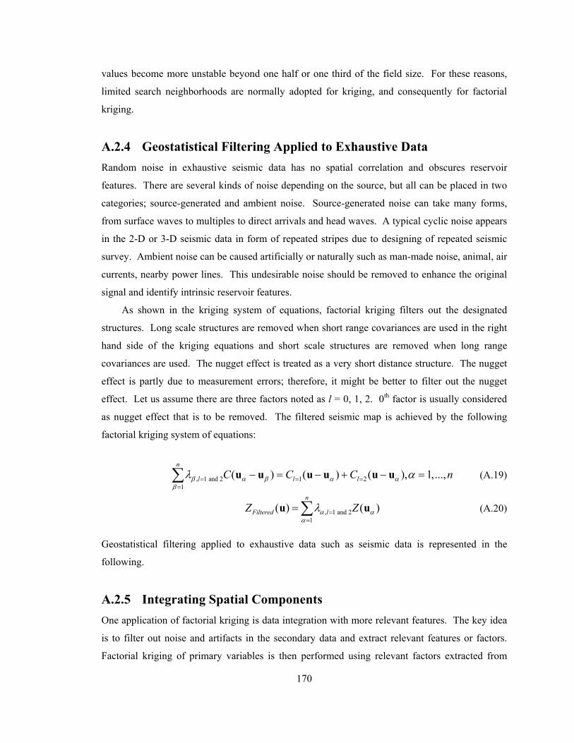
170

values become more unstable beyond one half or one third of the field size. For these reasons,

limited search neighborhoods are normally adopted for kriging, and consequently for factorial

kriging.

A.2.4 Geostatistical Filtering Applied to Exhaustive Data Random noise in exhaustive seismic data has no spatial correlation and obscures reservoir

features. There are several kinds of noise depending on the source, but all can be placed in two

categories; source-generated and ambient noise. Source-generated noise can take many forms,

from surface waves to multiples to direct arrivals and head waves. A typical cyclic noise appears

in the 2-D or 3-D seismic data in form of repeated stripes due to designing of repeated seismic

survey. Ambient noise can be caused artificially or naturally such as man-made noise, animal, air

currents, nearby power lines. This undesirable noise should be removed to enhance the original

signal and identify intrinsic reservoir features.

As shown in the kriging system of equations, factorial kriging filters out the designated

structures. Long scale structures are removed when short range covariances are used in the right

hand side of the kriging equations and short scale structures are removed when long range

covariances are used. The nugget effect is treated as a very short distance structure. The nugget

effect is partly due to measurement errors; therefore, it might be better to filter out the nugget

effect. Let us assume there are three factors noted as l = 0, 1, 2. 0th factor is usually considered

as nugget effect that is to be removed. The filtered seismic map is achieved by the following

factorial kriging system of equations:

, 1 and 2 1 21

( ) ( ) ( ), 1,...,n

l l lC C C nβ α β α αβ

λ α= = ==

− = − + − =∑ u u u u u u (A.19)

, 1 and 21

( ) ( )n

Filtered lZ Zα αα

λ ==

= ∑u u (A.20)

Geostatistical filtering applied to exhaustive data such as seismic data is represented in the

following.

A.2.5 Integrating Spatial Components

One application of factorial kriging is data integration with more relevant features. The key idea

is to filter out noise and artifacts in the secondary data and extract relevant features or factors.

Factorial kriging of primary variables is then performed using relevant factors extracted from

171

secondary data. For example, large scale features are often more important than locally variable

features. In this case, large scale features are extracted from the secondary data using simple

factorial kriging. The extracted secondary features are then used as a secondary data in order to

estimate primary variable, that is:

*,

1

( ) ( ) ( )n

l l l lZ Z Yα αα

λ ν=

= +∑u u u (A.21)

where *( )lZ u is an estimated primary variable for the l factor. λα,l are the weights assigned for

data samples to estimate l factor. Yl(u) is the extracted relevant secondary factor at collocation u.

lν is the weight assigned for secondary factor Yl(u) at estimation location u.

This method may be called factorial collocated cokriging since the only collocated secondary

factor is retained to estimate. The weights are obtained by solving collocated cokriging equations

for l factor.

1

1

,1

,1

( ) ( ) ( ) ( ), 1,...,

( ) ( ) (0) (0)

l

l l l l

nl

l ZZ l ZY ZZ

n

l Y Z l Y Y Y Z

C C C n

C C C

β α β α αβ

β ββ

λ ν α

λ ν

=

=

⎧− + − = − =⎪

⎪⎨⎪ − + =⎪⎩

∑

∑

u u u u u u u

u u u (A.22)

where Yl is the extracted lth component from the secondary data.

A.3 Experimental Results

To illustrate the usefulness of factorial kriging, synthetic data and real data are tested. The first

example is a synthetic regular grid data. Synthetic 256×256 2-D Gaussian variables are simulated

with a small nugget effect (10%) and two isotropic spherical structures equally explaining the

remaining 90% of the variability. Simulated values have stationary zero mean and unit variance.

The ranges of the spherical structures are 16 and 64 units. Data were sampled from the reference

grid at a very close 5×5 spacing to produce sample data so that total 2601 data were stored. The

modeled variogram for generating Gaussian variables is used as the fitted variogram using regular

sample data. The reference grid, sample data and used variogram are shown on Figure A.2. No

obvious anisotropic spatial features are observed in the reference map.

Ordinary factorial kriging estimates the mean and each factor independently. In this first

example the mean and three factors are to be estimated with ordinary factorial kriging. Maps of

172

the estimated factors are shown on Figure A.2. The nugget factor is non-zero at the data locations

and constant at all other locations. The nugget factor has no spatial structure. Note that the color

scale is changed to visualize the variability of the long range factor. Note that the estimate of the

mean reflects the most variability because of the unbiasedness constraints which forces the sum

of the weights to be 0 for each factor. Although the kriging equations and unbiasedness condition

achieve unbiasedness, it is unrealistic that the estimated mean factor has the majority of the

variability. Furthermore, the estimated long range structure has unreasonably low variability, as

shown in Figure A.2. Recall that the modeled variogram showed that the long range structure

contributes 45% of the total variability. The long scale features are mainly captured by the mean

factor. The short range estimated factor appears to vary within short distances. The sum of the

estimate of each factor adds up to the ordinary kriging estimate.

Figure A.2: The used variogram for generating simulation values (zero mean and unit variance Gaussian value), simulated values (bottom left) and sampled data (bottom right) are shown.

The ordinary kriging estimates are shown in the right bottom of Figure A.3 and it is ensured that

sum of all factor estimates reproduced data exactly.

173

Figure A.3: Estimated factors using ordinary factorial kriging. Mean, nugget, short scale and long scale factors are estimated. Sum of the estimated factors exactly reproduce ordinary kriging estimate over every grids.

The simple factorial kriging estimates of each factor are shown in Figure A.4. The same

kriging parameters such as search radius, minimum (8) and maximum number (18) of

conditioning data, are used except unconstrained kriging weights. The mean value is assumed to

174

be constant. The nugget, isotropic short range and long range factors are estimated and shown in

Figure A.4. The short range factor estimates appear to have variability within short distance and

long range factor estimates appear to have variability over large distances. The simple factorial

estimates reflect realistic features contrary to the ordinary factorial kriging estimates. A clear

improvement in feature identification of short scale and large scale spatial components through

simple factorial kriging is observed. The sum of all estimated factors reproduces the simple

kriged estimate as derived in Equations (A.14) and (A.18). Table 1 shows the variance of each

estimated factor by ordinary and simple factorial kriging, respectively. The variance table shows

the significant difference between ordinary and simple factorial estimates. The numeric values

show the calculated variance for each factor. The first column is the contribution of each factor

obtained by nested variogram modeling (shown in Figure A.1). The second and third columns

show the variance of each estimated factor with OFK and SFK. The last column in Table 1

shows how much OFK smoothes the estimated factors compared to SFK. The estimated mean

factor using OFK has 70% variability which is the majority of variability. SFK has more

variability than OFK and SFK produces more reasonable results in terms of feature identification.

Smoothing still exists in the SFK estimates, but not to the extent of OFK.

175

Figure A.4: Estimated factors using simple factorial kriging. Sum of the estimated factors and simple kriging estimate are shown as well.

Table A.1: Variance table for each estimated factor by OFK and SFK using the first synthetic example.

Factors bl = (al2) OFK SFK diff in %

mean – 0.7 0 (constant) – l = 0 (nugget) 0.1 0.0 0.0 0

l = 1 (short range) 0.45 0.25 0.55 25 l = 2 (long range) 0.45 0.05 0.45 98

176

The second example (cluster.dat) is from Deutsch and Journel (1998). The example contains

irregularly spaced well data over an area of 50×50 distance units. 140 clustered samples were

used for the analysis. The data values are first transformed to be Gaussian unit using normal

score transformation before applying factorial kriging. The locations of the normal score values

are shown in the left of Figure A.5. The omnidirectional variogram was modeled since there is

no obvious anisotropy. Three nested variogram structures were used; 20% nugget structure (very

short distance), 40% short range and 40% long range structure (Figure A.5). In some areas, high

values and low values are clustered with short distance, which contributes to the 40% short range

structure in the variogram. Factorial kriging results should recognize this short scale as well as

long scale. Ordinary factorial kriging was performed first. Figure A.6 illustrates four estimated

factors in normal score units: mean, nugget, short range and long range factors. Just like in the

first synthetic example, the mean factor has the majority of the variability. The nugget factor

estimates only exist at the data locations. The short range factors have variability within short

distances; however, the long range features are not clearly identified. The simple factorial kriging

estimated factors are shown in Figure A.7. The simple factorial kriging estimates appear more

reasonable.

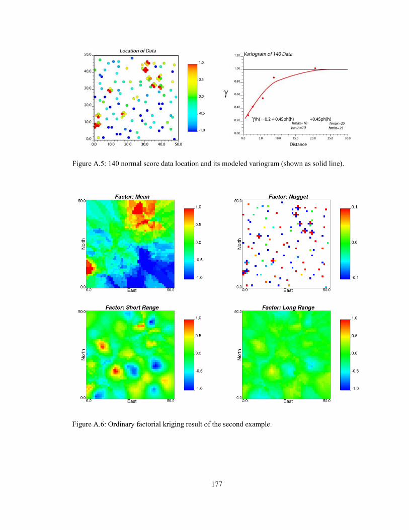
177

Figure A.5: 140 normal score data location and its modeled variogram (shown as solid line).

Figure A.6: Ordinary factorial kriging result of the second example.

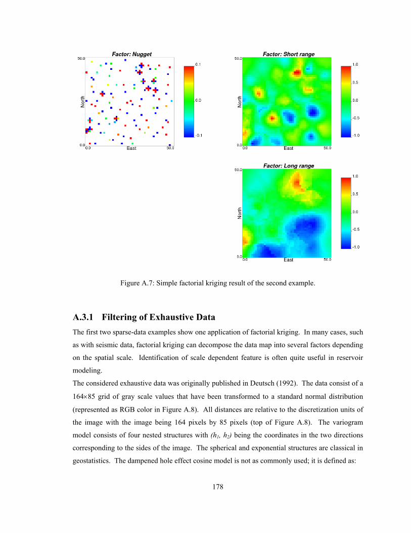
178

Figure A.7: Simple factorial kriging result of the second example.

A.3.1 Filtering of Exhaustive Data

The first two sparse-data examples show one application of factorial kriging. In many cases, such

as with seismic data, factorial kriging can decompose the data map into several factors depending

on the spatial scale. Identification of scale dependent feature is often quite useful in reservoir

modeling.

The considered exhaustive data was originally published in Deutsch (1992). The data consist of a

164×85 grid of gray scale values that have been transformed to a standard normal distribution

(represented as RGB color in Figure A.8). All distances are relative to the discretization units of

the image with the image being 164 pixels by 85 pixels (top of Figure A.8). The variogram

model consists of four nested structures with (h1, h2) being the coordinates in the two directions

corresponding to the sides of the image. The spherical and exponential structures are classical in

geostatistics. The dampened hole effect cosine model is not as commonly used; it is defined as:

179

, ( ) 1.0 exp cos( )d ahaDH h had−⎛ ⎞= − ⎜ ⎟

⎝ ⎠ (A.23)

There are four components in the variogram model that correspond to factors in the interpretation

of factorial kriging:

1. A short scale anisotropic spherical structure that explains 45% of the total variability

(the longer range is in the horizontal h2 direction and the shorter range is in the

vertical h1 direction).

2. A second short scale anisotropic spherical structure (with a more pronounced

anisotropy along the same horizontal and vertical directions) that explains an

additional 22% of the variability,

3. A third anisotropic long range exponential structure (the range parameter is 40.0,

thus, the effective range is 120.0 in the horizontal direction and 0.0 in the vertical

direction ) that explains 45% of the variability, and

4. Finally, a dampened hole effect model in the vertical direction to account for the

periodicity.

The modeled variogram is shown at the bottom of Figure A.8.

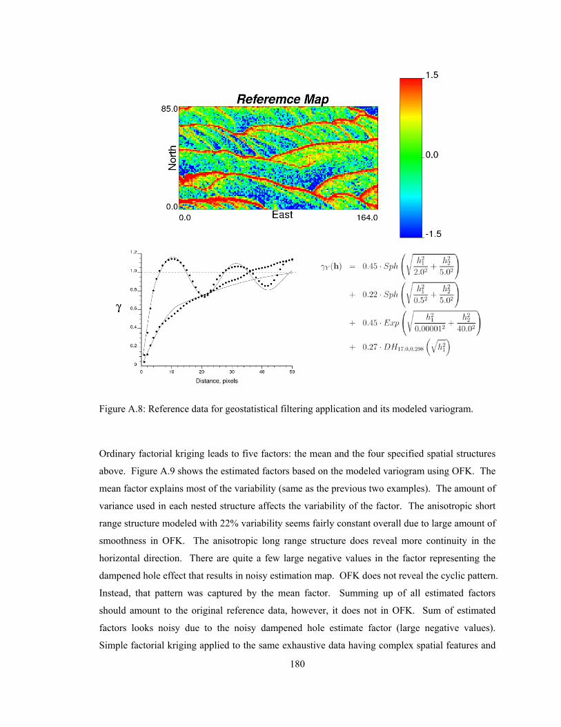
180

Figure A.8: Reference data for geostatistical filtering application and its modeled variogram.

Ordinary factorial kriging leads to five factors: the mean and the four specified spatial structures

above. Figure A.9 shows the estimated factors based on the modeled variogram using OFK. The

mean factor explains most of the variability (same as the previous two examples). The amount of

variance used in each nested structure affects the variability of the factor. The anisotropic short

range structure modeled with 22% variability seems fairly constant overall due to large amount of

smoothness in OFK. The anisotropic long range structure does reveal more continuity in the

horizontal direction. There are quite a few large negative values in the factor representing the

dampened hole effect that results in noisy estimation map. OFK does not reveal the cyclic pattern.

Instead, that pattern was captured by the mean factor. Summing up of all estimated factors

should amount to the original reference data, however, it does not in OFK. Sum of estimated

factors looks noisy due to the noisy dampened hole estimate factor (large negative values).

Simple factorial kriging applied to the same exhaustive data having complex spatial features and

181

factor estimation results are shown in Figure A.10. Cyclic pattern of data is significant in the

estimated dampened hole factor. Sum of estimated factors amounts to the reference image. One

of possible extension of factorial kriging to exhaustive data set is to filter out the undesired spatial

features. For example, repetitive seismic survey may invoke periodic systematic noise which is

better to be removed to enhance the clarity of the data. The considered data has contains cyclic

spatial features that is mainly characterized as dampened hole effect in the variogram. We treated

the data as seismic data interrupted with cyclic noise. Thus, that feature is to be removed for

enhancing signal-to-noise ratio of seismic data. Cyclicity filtered image is simply derived from

summing of the other estimated factors. In OFK, sum of mean, two anisotropic short range,

anisotropic long range factors is equivalent to the cyclicity filtered image. In SFK, sum of two

anisotropic short range, anisotropic long range factor is equivalent to the filtered image. Two

filtered image are compared in Figure A.11 and it should be noted that SFK shows better

performance in terms of removing periodic structure. Geostatistical filtering is basically

depending on the number and types of fitted variogram. This is one advantage of geostatistical

filtering technique since geologic knowledge can be added when fitting the experimental

variogram hence more realistic structure may be extracted.

182

Figure A.9: Factor estimate of the exhaustive data using ordinary factorial kriging.

183

Figure A.10: Factor estimate of the exhaustive data using simple factorial kriging. Note that summing up of all estimated factors amounts to the reference map shown Figure A.7.

184

Figure A.11: Cyclic spatial feature is filtered out by OFK and SFK. SFK alleviates the pattern which we assumed noise inherent in data.

A.3.2 Combining Spatial Components

Another application of factorial kriging is to integrate relevant features with primary data.

Factorial kriging can filter out unwanted spatial features depending on the purpose of study.

Filtered secondary data then can be used as a new secondary data to be combined with primary.

Another petroleum field data (Amoco.dat) is tested for factorial data integration (Deutsch and

Journel, 1998). We have one primary porosity variable to be estimated and one exhaustively

sampled seismic-derived acoustic impedance. Secondary data is sampled by 65 × 65 with 160

unit distance. Variables were first transformed into normal space. Modeled variogram of

porosity provide two identified spatial features, i.e. 20% isotropic small scale and 70%

anisotropic large scale features (major direction in N-S and minor direction in E-W).

hmin=hmax 1000 hmin=5000hmax=17000

( ) 0.2 ( ) 0.8 ( )Sph Sphγ == +h h h (A.24)

Secondary variable appears to vary smoothly over the domain. The variogram of the secondary

data is fitted with two features: 25% isotropic small scale and 75% isotropic large scale features.

Anisotropic direction of secondary variable is same as primary variable: major in N-S and minor

in E-W.

hmin=hmax 1000 hmin=4000hmax=10000

( ) 0.25 ( ) 0.75 ( )Sph Sphγ == +h h h (A.25)

Maps of the primary and secondary data are shown in Figure A.12 with the variograms. No

nugget filtering is required since the variogram has no nugget contribution. Simple factorial

185

kriging with exhaustive secondary data was performed and two factors are extracted separately:

isotropic small scaled feature and isotropic large scaled feature. To check the relationships

between primary porosity and extracted factors, correlation coefficient is calculated. Let us

clarify the notation: Z is primary variable (normal score value), Ytotal is original secondary

variable (normal score value), Yl=1 and Yl=2 are factor 1 and factor 2 extracted from secondary

variable. Correlation (ρZY) of primary Z and total secondary variable Ytotal is 0.615. It is noted

that correlation coefficient is slightly changed when plotting extracted factor 1 and 2 with primary

variable,

10.34 0.615

l totalZY ZYρ ρ== < =

20.65 0.615

l totalZY ZYρ ρ== > =

The large scale factor is highly correlated to the primary variable. This is a reasonable result

since the variogram of primary porosity has greater contribution of large scale feature (80%

variability) than small scale feature (20% variability). Besides, the variogram of seismic data

shows 75% variability contribution of large scale feature. There are two evident options for data

integration. One option is to use extracted relevant factor as a new secondary variable. Simple

cokriging is applied to the primary variable using the new secondary data (extracted relevant

factor). The second factor is used as secondary data. This factor is transformed into normal

scores. In this integration option, the long range structure is enhanced and short range structure is

weakened because large scale feature is imposed both by primary (80%) and secondary data

(75%), but small scale feature is imposed only by primary data (20%). The other option is to

apply simple factorial cokriging to the primary variable using the extracted relevant secondary

variable. Equation (A.22) explains the latter option.

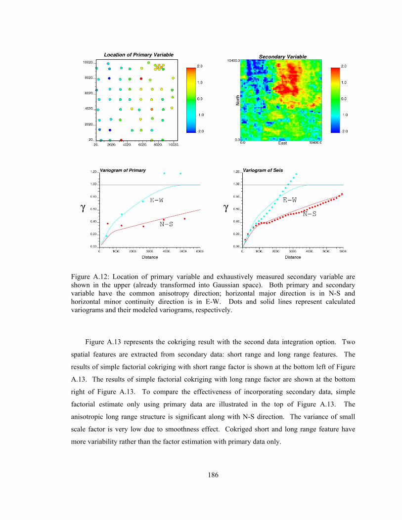
186

Figure A.12: Location of primary variable and exhaustively measured secondary variable are shown in the upper (already transformed into Gaussian space). Both primary and secondary variable have the common anisotropy direction; horizontal major direction is in N-S and horizontal minor continuity direction is in E-W. Dots and solid lines represent calculated variograms and their modeled variograms, respectively.

Figure A.13 represents the cokriging result with the second data integration option. Two

spatial features are extracted from secondary data: short range and long range features. The

results of simple factorial cokriging with short range factor is shown at the bottom left of Figure

A.13. The results of simple factorial cokriging with long range factor are shown at the bottom

right of Figure A.13. To compare the effectiveness of incorporating secondary data, simple

factorial estimate only using primary data are illustrated in the top of Figure A.13. The

anisotropic long range structure is significant along with N-S direction. The variance of small

scale factor is very low due to smoothness effect. Cokriged short and long range feature have

more variability rather than the factor estimation with primary data only.

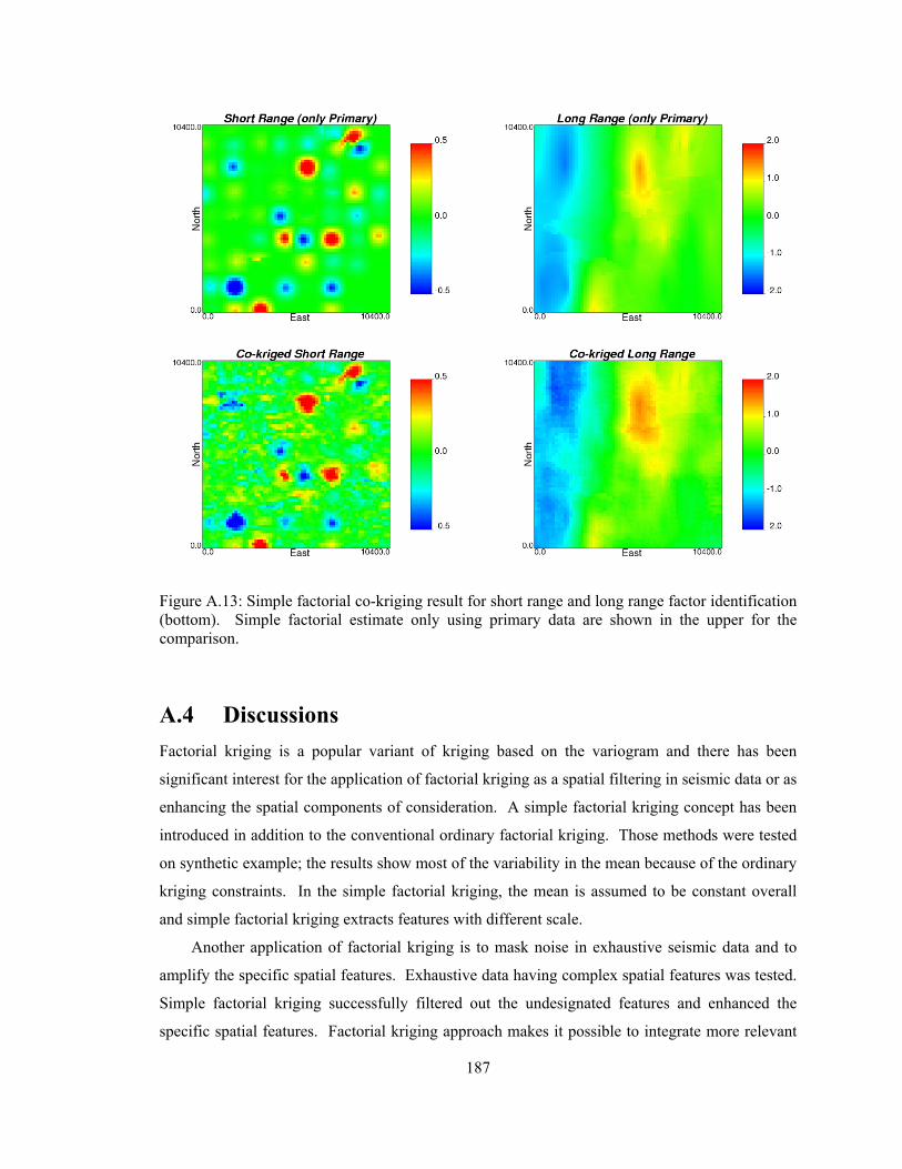
187

Figure A.13: Simple factorial co-kriging result for short range and long range factor identification (bottom). Simple factorial estimate only using primary data are shown in the upper for the comparison.

A.4 Discussions

Factorial kriging is a popular variant of kriging based on the variogram and there has been

significant interest for the application of factorial kriging as a spatial filtering in seismic data or as

enhancing the spatial components of consideration. A simple factorial kriging concept has been

introduced in addition to the conventional ordinary factorial kriging. Those methods were tested

on synthetic example; the results show most of the variability in the mean because of the ordinary

kriging constraints. In the simple factorial kriging, the mean is assumed to be constant overall

and simple factorial kriging extracts features with different scale.

Another application of factorial kriging is to mask noise in exhaustive seismic data and to

amplify the specific spatial features. Exhaustive data having complex spatial features was tested.

Simple factorial kriging successfully filtered out the undesignated features and enhanced the

specific spatial features. Factorial kriging approach makes it possible to integrate more relevant

188

feature with primary variable. We tested factorial collocated cokriging using sparely sampled

porosity and extracted relevant factor from seismic data. After factorial collocated cokriging, we

could clearly identify scale dependent structures compared with the factorial kriging with primary

only.