Multivariable Calculus

Module II: Optimization

Matthew F. Causley, Ruben Hayrepetyan, Allan TaylorKettering University

Contents

1 Introduction 2

2 Example: Supply and Demand for Vehicles 22.1 Exercise: Tomatoes and Peppers . . . . . . . . . . . . . . . . . . . . . . . . . . . . . . . . . . . . . 32.2 Reconsidering Rates of Change . . . . . . . . . . . . . . . . . . . . . . . . . . . . . . . . . . . . . . 32.3 Mini-project: The Maximum Problem . . . . . . . . . . . . . . . . . . . . . . . . . . . . . . . . . . 4

3 Project: Cobb-Douglas Function 53.1 Production Function and Revenue . . . . . . . . . . . . . . . . . . . . . . . . . . . . . . . . . . . . 53.2 Maximum Profit . . . . . . . . . . . . . . . . . . . . . . . . . . . . . . . . . . . . . . . . . . . . . . 5

4 Constrained Optimization: The Method of Lagrange Multipliers 6

5 Project: Elasticity 75.1 Maximum Normal Stress . . . . . . . . . . . . . . . . . . . . . . . . . . . . . . . . . . . . . . . . . . 85.2 Maximum Shear Stress . . . . . . . . . . . . . . . . . . . . . . . . . . . . . . . . . . . . . . . . . . . 8

6 Project: Lagrange Multiplers, and Sufficient Conditions 8

7 Project: Economics 97.1 Maximum Production . . . . . . . . . . . . . . . . . . . . . . . . . . . . . . . . . . . . . . . . . . . 9

8 Example: Maximum Power Transfer Theorem 108.1 DC Circuits . . . . . . . . . . . . . . . . . . . . . . . . . . . . . . . . . . . . . . . . . . . . . . . . . 108.2 AC Circuits . . . . . . . . . . . . . . . . . . . . . . . . . . . . . . . . . . . . . . . . . . . . . . . . . 11

9 Project: Electrical Component Tolerance 129.1 Band-Pass Filtering . . . . . . . . . . . . . . . . . . . . . . . . . . . . . . . . . . . . . . . . . . . . 129.2 Component Tolerance Optimization . . . . . . . . . . . . . . . . . . . . . . . . . . . . . . . . . . . 13

1

1 Introduction

In this module we discuss optimization problems, their applications, and methods of solution. Optimizationproblems, i.e. problems of finding maxima and minima of functions, are among the most important problemsin mathematics. They have extremely important applications in economics, engineering, and science. Westart with one optimization problem originating in economics, and illustrate the basic ideas employed inthe mathematical methods of solution. At the beginning we use simple reasoning rather than rigorous calculuslanguage. The more rigorous techniques are gradually introduced later.

2 Example: Supply and Demand for Vehicles

You work for a dealership that sells two types of vehicles: trucks and sedans. You are responsible for pricing, andhave to choose the prices that maximize the revenue. To solve the problem you need a mathematical model ofsales. This is not a simple task; there are many factors that affect sales. So first of all you have to make somesimplifying assumptions. Let us assume that there are no other dealerships around, so you are very lucky not tohave competitors! Additionally, assume you have enough cars to completely satisfy the demand. Then the revenueis governed by price-demand equations.

Denote by x the price of a truck, by y the price of a sedan, by t and s the demands per month on trucks andsedans. After analyzing the market you have come up with the following price-demand equations:

t = 10, 000− 2x+ 2.5y, (1)

s = 16, 000 + 1.5x− 3y. (2)

These equations reflect a simple observation that when the price of trucks increases then customers buy fewertrucks and more sedans, and when the price on sedans increases they buy more trucks and fewer sedans.

Assuming that the dealership sells t trucks at a price of x dollars per truck and s sedans at a price of y dollarsper sedan the revenue of the dealership would be

R = tx+ sy = (10, 000− 2x+ 2.5y)x+ (16, 000 + 1.5x− 3y)y. (3)

In this model the revenue R is a function of two variables x and y. Simplifying the left hand side term in (3)we see that the revenue can be expressed in terms of the following quadratic function of two independent variablesx and y:

R(x, y) = −2x2 − 3y2 + 4xy + 10, 000x+ 16, 000y. (4)

Now we can state our task of finding prices that maximize the revenue as a mathematical problem:

Optimization problem. Find values of x and y such that R(x, y) achieves its maximal value.

Later we will see how calculus solves this problem. Now we try to solve it using simple reasoning only. As wealways do in mathematics let us denote the unknown solution of this problem by x0, y0 and try to find equationsfor them. That is, let us assume that R(x, y) achieves its maximal value at some point (x0, y0).

Our solution is based on the following simple idea: though both x and y are variables and their values change,it does not mean that they have to change simultaneously. First let us keep the price of sedans constantand equal to y0, that is y = y0, and change only the price of trucks. Since y = y0 is fixed, the revenue is a functionof only x. Let us denote this function by

g(x) = R(x, y0) = −2x2 − 3y20 + 4xy0 + 10, 000x+ 16, 000y0. (5)

Now let us find the price x0 that maximizes the function of one variable g(x) using the method from Calculus Ithat treats optimization problems for single variable functions. We know that the maximum is achieved at thepoint x0 where the first derivative equals zero:

g′(x0) = −4x0 + 4y0 + 10, 000 = 0. (6)

2

Now let us fix x = x0 and find the value of y for which R(x0, y) is maximal. After fixing x = x0 in (4) we get afunction of a single variable y:

h(y) = R(x0, y) = −2x20 − 3y2 + 4x0y + 10, 000x0 + 16, 000y. (7)

In order to find the maximal value of h(y) we use the Calculus I again:

h′(y0) = −6y0 + 4x0 + 16, 000 = 0. (8)

Combining equations (6) and (8) we get the following system of two equations:{−4x0 + 4y0 + 10, 000 = 0−6y0 + 4x0 + 16, 000 = 0.

(9)

This system can be solved by the elimination method. From the first equation 4x0 = 4y0 + 10, 000 or

x0 = y0 + 2, 500. (10)

Substituting it in the second equation we obtain

− 6y0 + 4(y0 + 2, 500) + 16, 000 = 0. (11)

Therefore,− 6y0 + 4y0 + 10, 000 + 16, 000 = 0, (12)

andy0 = 13, 000. (13)

Correspondingly,x0 = y0 + 2, 500 = 15, 500. (14)

So if the maximum of the function R(x, y) exists, it is achieved at x0 = 15, 500, y0 = 13, 000.Based on this mathematical model you may suggest the following prices: $15, 500 for a truck and $13, 000 for

a sedan.Remark. We have solved the problem assuming from the very beginning that the maximum of R(x, y) exists.

For our dealership problem it seems to be a reasonable assumption. Many optimization problems that appear inapplications allow us to make such assumptions.

2.1 Exercise: Tomatoes and Peppers

A company produces tomatoes and peppers and sells them at prices $2 per pound for tomatoes and $3 per poundfor peppers. The cost of production of x pounds of tomatoes and y pounds of peppers is C(x, y) = x2 + 3xy+ y2.The revenue from selling x pounds of tomatoes and y pounds of peppers is R(x, y) = 2x + 3y and the profit isP (x, y) = R(x, y) − C(x, y). How many tomatoes and peppers should the company produce to get the maximalprofit?

2.2 Reconsidering Rates of Change

We have successfully solved the problem of a dealership stated in the preceding example. Now let us analyze thebasic idea that has allowed us to solve the problem. Similar to ideas of Calculus I, our solution was based oninstantaneous rates of change. In Calculus I an instantaneous rate of change is called a derivative and canbe found by differentiation. However, in Calculus I only functions of one variable were considered. The functionR(x, y) considered in the Example 1 depends on two variables x and y. This was a reason why in the solution weslightly modified the concept of an instantaneous rate of change. As a matter of fact we used two different rates ofchange: the rate of change with respect to x with fixed y and the rate of change with respect to y with fixedx. Mathematically this procedure can be described as follows. In order to find the first rate of change, simplytreat y as a constant (fixed) so your function becomes only depends on x, and apply differentiation to this functionof one variable. Similarly, to find the second rate of change treat x as a constant and apply differentiation to the

3

function of one variable y. Rates of change obtained by using this procedure are called partial derivatives todistinguish them from derivatives of functions of one variable. (Derivatives of functions of one variable are oftencalled ordinary derivatives.)

So, if there is a function of two variables f(x, y), then two rates of change should be considered: a rate ofchange with respect to x and a rate of change with respect to y. In other words, to find a partial derivative withrespect to x assume that y is fixed (constant) and differentiate with respect to x, and to find a partial derivativewith respect to y assume that x is fixed and differentiate with respect to y. The following notations for partialderivatives are used:

∂f(x, y)

∂xor fx(x, y),

∂f(x, y)

∂yor fy(x, y).

Finding maxima is like climbing mountains. You are looking for a point where the elevation is maximal. Soit is a point at which the rate of change of elevation changes its sign from positive (when you go up the elevationincreases) to negative (when you go down the elevation decreases). So at a maxima point (the top of the mountain)all rates of change of elevation should change their sign from positive to negative. Therefore if these rates aredefined they should equal zero at a maxima point.

In other words, if f(x, y) is differentiable and has a maximum at (a, b), then the following necessary conditionsshould be satisfied:

fx(a, b) = 0, fy(a, b) = 0. (15)

2.3 Mini-project: The Maximum Problem

In this mini-project you will derive necessary conditions (15) and then sufficient conditions for f(x, y) to have amaximum at (a, b). Your approach will be based on the theorems of Calculus I. The main idea is to reduce theproblem for a function of two variables, to one for a function of one variable and then apply the results fromCalculus I. Indeed, if f(x, y) has a maximum at (a, b) then for any line L passing throw (a, b) the function of onevariable that is the restriction of f(x, y) on L has a maximum at that point. To apply this idea follow the steps:

1. Let us assume that f(x, y) has a maximum at (a, b). Write an equation of the line in xy-plane with slope mthat passes throw the point(a, b).

2. Write the function g(x) that is a restriction of f(x, y) on the line from the Step 1.

3. Use the Chain Rule to find the derivative of g(x).

4. Apply the necessary condition g′(a) = 0.

5. Use the equation g′(a) = 0 with arbitrary m to derive conditions (15).

6. Use the Chain Rule again to find the second derivative of g(x).

7. Apply the sufficient condition g′′(a) < 0.

4

8. Use the inequality g′′(a) < 0 with arbitrary m to derive the following sufficient conditions:

fxx(a, b) < 0, fxxfyy − f2xy > 0 (16)

are sufficient for having a maximum at (a, b).

9. Repeat the Steps 6-8 to find sufficient conditions for having a minimum at (a, b).

10. (Optional) Repeat the Steps 1-9 replacing line L by an arbitrary curve h(x, y) = 0 passing through (a, b).

3 Project: Cobb-Douglas Function

Definitions

In this project you will need some basic definitions from economics. You can use books or internet resources suchas Wikipedia.

In the first section of your project define and explain the Cobb-Douglas production function.

3.1 Production Function and Revenue

Assume that you are a manager of a company. Your goal is to maximize the profit P of your company. Theproduction of your company can be modeled by the following Cobb-Douglas function:

P = CKaLbM c, a > 0, b > 0, c > 0.

where $K is capital stocks (the monetary worth of all machinery, equipment, and buildings), $L is labor input(the total number of person-hours worked in a year), $M is materials and supplies, and C is a given productivitycoefficient.

You may assume that a+ b+ c = 1. Discuss this assumption from the point of view of economics. (You mayuse books or internet resources.)

3.2 Maximum Profit

Assuming that the unit price for the product you produce is $ p, your revenue is

R = pCKaLbM c,

the production cost is L+M , and the profit is

f(L,M) = pCKaLbM c − L−M.

Here we assume that the capital stocks K is fixed but you can control the labor cost L and materials and suppliescost M .

Your goal is to choose L and M that maximize the profit.

Justification

After you presented your budget to maximize the profit some members of the board of directors were not convinced.They asked you to justify your decisions and to prove that the proposed budget will give the maximal profit. Usethe second derivative test to justify your decision.

Examples and Applications

Discuss numerical examples. Describe possible applications of your results.

5

References

Include all sources you used. For example:

1. C.W. Cobb and P.H.Douglas, A theory of production. American Economic Review 18(1):139165. Supplement,Papers and Proceedings of the Fortieth Annual Meeting of the American Economic Association, 1928.

4 Constrained Optimization: The Method of Lagrange Multipliers

In the previous section the problem of unconstrained optimization was discussed. The goal of this section isto develop the method for solving constrained optimization problems, that is to find maxima and minima of afunction subject some additional conditions (constraints).

An introductory example. Let us consider the following problem: find the extrema of f(x, y, z) = xy +2x− 3y − z + 3 on the surface of the paraboloid x2 + y2 − z = 1, that is

f(x, y, z) = xy + 2x− 3y − z + 3→ extremum, (17)

g(x, y, z) = x2 + y2 − z − 1 = 0. (18)

The solution of this problem may not be (and in general is not) a critical point of f(x, y, z). So the methods ofthe previous section are not applicable here.

However, this problem can be immediately reduced to a problem of unconstrained optimization if one solvesequation (18) with respect to z:

z = x2 + y2 − 1

and then substitutes it into the function f to obtain the following unconstrained optimization problem:

h(x, y) := f(x, y, x2 + y2 − 1) = xy − x2 − y2 + 2x− 3y + 4→ extremum.

The resulting problem can be easily solved by setting the first partial derivatives hx and hy equal zero.In Example 2 a successful reduction to a problem without constraint was possible only because one was able

to solve equation (18) with respect to z. However, in the many important problems of constrained optimizationthe equation representing the constrain cannot be explicitely solved with respect to x, y, or z.

The brilliant idea of Lagrange was that the constrained optimization problem{f(x, y, z)→ extremumg(x, y, z) = 0

(19)

still can be reduced to a problem of finding critical points of some function.To illustrate the method of Lagrange we will follow the same procedure as in the previous example. The only

difference is that this time we will use implicit differentiation. We will assume that ∇g(x, y, z) 6= 0. Then, theequation g(x, y, z) = 0 allows one to express one of the variables x, y, or z as an implicit function of two others.For instance, let gz(x, y, z) 6= 0 and assume that such a function is z = z(x, y). Substituting this function into fone gets an optimization problem without a constraint

h(x, y) = f(x, y, z(x, y))→ extremum.

The solutions of this problem are among the critical points of function g(x, y). Therefore we are looking forsolutions of the following system of equations: {

∂h(x,y)∂x = 0

∂h(x,y)∂y = 0.

(20)

Now applying the implicit differentiation to g(x, y, z) = 0, we get

∂z

∂x= −gx(x, y, z)

gz(x, y, z),

∂z

∂y= −gy(x, y, z)

gz(x, y, z).

6

The next step is to find the derivatives hx(x, y) and hy(x, y) by applying the Chain Rule to h(x, y) = f(x, y, z(x, y)):

∂h

∂x=∂f

∂x+∂f

∂z

∂z

∂x=∂f

∂x− ∂f

∂z

gx(x, y, z)

gz(x, y, z),

∂h

∂y=∂f

∂y+∂f

∂z

∂z

∂y=∂f

∂y− ∂f

∂z

gy(x, y, z)

gz(x, y, z).

Substituting these expressions into equations (20) we obtain{∂f∂x −

∂f∂z

gx(x,y,z)gz(x,y,z)

= 0,∂f∂y −

∂f∂z

gy(x,y,z)gz(x,y,z)

= 0.

Thus, if the point (x0, y0) is a solution of the system (20) and z0 = z(x0, y0), then{∂f∂x (x0, y0, z0)− ∂f

∂z (x0, y0, z0)gx(x0,y0,z0)gz(x0,y0,z0)

= 0,∂f∂y (x0, y0, z0)− ∂f

∂z (x0, y0, z0)gy(x0,y0,z0)gz(x0,y0,z0)

= 0.(21)

Denote

λ =fz(x0, y0, z0)

gz(x0, y0, z0), (22)

then equations (21) imply {fx(x0, y0, z0)− λgx(x0, y0, z0) = 0,fy(x0, y0, z0)− λgy(x0, y0, z0) = 0.

(23)

Combining these equations with the equation (22) we get

∇f(x0, y0, z0) = λ∇g(x0, y0, z0). (24)

Therefore, if the point (x0, y0, z0) is a solution to the problem (19), then there exists a number λ such that(x0, y0, z0, λ) is a solution to the system of equations:{

∇f(x, y, z) = λ∇g(x, y, z),g(x, y, z) = 0.

(25)

Following Lagrange, let us introduce the function

L(x, y, z, λ) = f(x, y, z)− λg(x, y, z), (26)

that is called the Lagrange function. It is easy to see that if one sets the first partial derivatives of the Lagrangefuction Lx, Ly, Lz, and Lλ equal zero, one obtains the system (25).

Thus, we can claim that the solutions to the constrained optimization problem (19) are among the criticalpoints of the function L defined in (27).

5 Project: Elasticity

Definitions

For this project you will need some basic definitions from the Theory of elasticity. You can use books or internetresources such as Wikipedia.

In the first section of your project define and explain the concepts of Strain, Stress, Normal Stress, ShearStress, Maximum Shear Stress Plane, Maximum Shear Stress Angle.

7

5.1 Maximum Normal Stress

In stress analysis problems, one is interested in finding the maximum and minimum normal stresses, and themaximum shearing stress at a point. Explain why it is important.

In the following discussion, the point x in the present configuration is kept fixed.At the point x in the present configuration of the body, consider a plane whose outer unit normal is n =<

n1, n2, n3 >. The stress vector on this plane is given by equation

T =< σ11n1 + σ12n2 + σ13n3, σ21n1 + σ22n2 + σ23n3, σ31n1 + σ32n2 + σ33n3 >,

where

σ =

σ11 σ12 σ13σ21 σ22 σ23σ31 σ32 σ33

is a stress tensor. The stress tensor can be reduced to a symmetrical form. So you may assume that

σ21 = σ12, σ31 = σ13, σ32 = σ23.

The normal stress on this plane is given by

Tnormal = compnT = T · n.

Thus the problem of finding the maximum or the minimum normal stress at the point x reduces to findingthe unit vector n for which σnormal is maximum or minimum. So you are looking for a solution to the followingconstrained optimization problem:

Tnormal(n1, n2, n3)→ extremum,

n21 + n22 + n23 = 1.

Use Lagrange Multipliers method to solve this problem.

5.2 Maximum Shear Stress

The shear stress on the plane with the normal vector n is given by the equation

T 2normal + T 2

shear = |T|2.

Find the expression for the shear stress.Use Lagrange Multipliers method to find the plane of the maximal shear stress.

Examples and Applications

Discuss numerical examples. Describe possible applications of your results.

References

Include all sources you used. For example:

1. S. Timoshenko and J.N. Goodier, Theory of Elasticity, McGRAW–HILL BOOK COMPANY, Inc. 1951.

6 Project: Lagrange Multiplers, and Sufficient Conditions

In this project you will derive sufficient conditions for the existence of a relative extremum in an optimizationproblem with one constraint: {

f(x, y)→ extremumg(x, y) = 0.

(27)

We assume that ∇g 6= 0 that is either gx 6= 0 or gy 6= 0. Let as assume that gy 6= 0. To derive the conditions,follow the steps:

8

1. The equation g(x, y) = 0 defines an implicit function y = y(x). Using implicit differentiation find y′(x) andy′′(x).

2. Introduce a function h(x) = f(x, y(x)). Show that if the point (a, b) is a solution to problem (27), then thepoint a is a relative extremum point for h(x).

3. Using the Chain Rule find h′(x) and h′′(x).

4. Substitute the expressions for y′(x) and y′′(x) into the expressions for h′(x) and h′′(x).

5. Show that the necessary condition h′(a) = 0 implies that there exists a number λ such that

∇f(a, b) = λ∇g(a, b).

6. Introduce the Lagrange function L(x, y, λ) = f(x, y)− λg(x, y) and show that

∇L(a, b, λ) = 0.

7. Substitute f(x, y) = L(x, y, λ) + λg(x, y) into the expression for h′′(x).

8. Apply the sufficient condition for relative minimum h′′(a) > 0 to derive sufficient condition for a minimumin problem (27).

9. Apply the sufficient conditions for relative maximum h′′(a) < 0 to derive sufficient conditions for a maximumin problem (27).

10. Express the sufficient conditions from steps 8 and 9 in terms of the following determinant:∣∣∣∣∣∣0 gx(a, b) gy(a, b)

gx(a, b) Lxx(a, b, λ) Lxy(a, b, λ)gy(a, b) Lxy(a, b, λ) Lyy(a, b, λ)

∣∣∣∣∣∣11. (Optional) Find sufficient conditions for a relative extremum in an optimization problem with one constraint:{

f(x, y, z)→ extremumg(x, y, z) = 0.

(28)

7 Project: Economics

Definitions

In this project you will need some basic definitions from economics. You can use books or internet resources suchas Wikipedia.

In the first section of your project define and explain the Cobb-Douglas production function.

7.1 Maximum Production

Assume that you are the manager of a plant. Your goal is to maximize the production P of your plant. Theproduction can be modeled by the following Cobb-Douglas function:

P = CLαMβT γ ,

where $L is labor input (the total number of person-hours worked in a year), $M is materials and supplies, $T isthe transportation cost, and C is a given productivity coefficient. All these expenses you should cover from yourfixed budget $B.

Use the Lagrange multipliers method to maximize the production of your plant by dividing your budget Bbetween L, M , and T .

9

Justification

After you presented your budget to maximize the production some members of the board of directors were notconvinced. They asked you to justify your decisions and to prove that the proposed budget will give the maximalproduction. Use the second derivative test to justify your decision.

Examples and Applications

Discuss numerical examples. Describe possible applications of your results.

References

Include all sources you used. For example:

1. C.W. Cobb and P.H.Douglas, A theory of production. American Economic Review 18(1):139165. Supplement,Papers and Proceedings of the Fortieth Annual Meeting of the American Economic Association, 1928.

8 Example: Maximum Power Transfer Theorem

8.1 DC Circuits

One problem that arises when studying DC electrical circuits is how to obtain maximum power transfer.Suppose we have a constant-voltage power source (e.g. a battery). We would like to know what size of electricalload can be placed across the battery terminals to extract the maximum amount of power from the battery. Wecan frame this mathematically as an optimization problem.

Our model of the battery consists of two parts: an ideal voltage source and a parasitic loss resistance.We will model the electrical load as an additional resistance. This basic battery-model-with-load circuit is shownin Figure (1), where VOC is the open-circuit voltage (measured in Volts), and RTh and RL are the parasitic andload resistors, respectively (in Ohms). The power PL consumed by the load is the product of the load voltage Vo

Figure 1: Circuit model of a battery

and the load current Io. Using Ohms Law, we relate it to the load resistance

PL = VoIo = Vo

(VoRL

)=V 2o

RL. (29)

However, Vo still depends on RL, which is the variable we will use to optimize PL. After applying more circuitanalysis, we obtain

PL =VOCRL

(RTh +RL)2. (30)

10

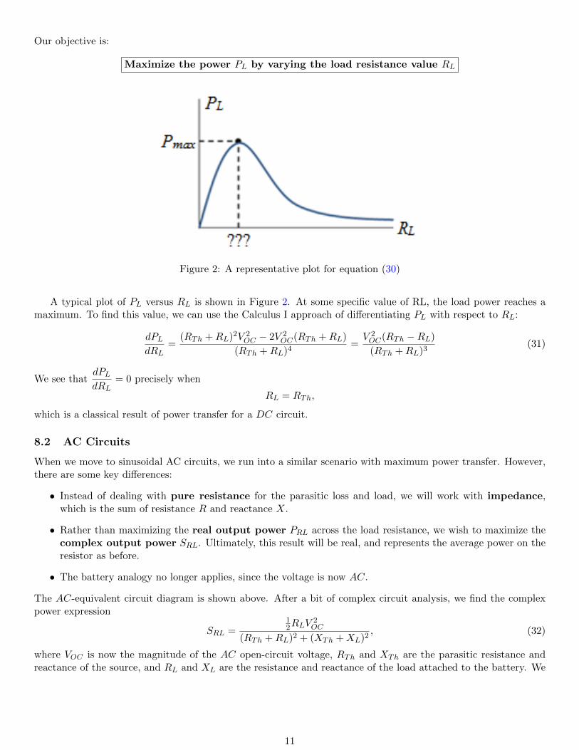
Our objective is:

Maximize the power PL by varying the load resistance value RL

Figure 2: A representative plot for equation (30)

A typical plot of PL versus RL is shown in Figure 2. At some specific value of RL, the load power reaches amaximum. To find this value, we can use the Calculus I approach of differentiating PL with respect to RL:

dPLdRL

=(RTh +RL)2V 2

OC − 2V 2OC(RTh +RL)

(RTh +RL)4=V 2OC(RTh −RL)

(RTh +RL)3(31)

We see thatdPLdRL

= 0 precisely when

RL = RTh,

which is a classical result of power transfer for a DC circuit.

8.2 AC Circuits

When we move to sinusoidal AC circuits, we run into a similar scenario with maximum power transfer. However,there are some key differences:

• Instead of dealing with pure resistance for the parasitic loss and load, we will work with impedance,which is the sum of resistance R and reactance X.

• Rather than maximizing the real output power PRL across the load resistance, we wish to maximize thecomplex output power SRL. Ultimately, this result will be real, and represents the average power on theresistor as before.

• The battery analogy no longer applies, since the voltage is now AC.

The AC-equivalent circuit diagram is shown above. After a bit of complex circuit analysis, we find the complexpower expression

SRL =12RLV

2OC

(RTh +RL)2 + (XTh +XL)2, (32)

where VOC is now the magnitude of the AC open-circuit voltage, RTh and XTh are the parasitic resistance andreactance of the source, and RL and XL are the resistance and reactance of the load attached to the battery. We

11

would like to maximize SRL in terms of both RL and XL, which we see is now a two-dimensional optimizationproblem. Thus, we will compute both partial derivatives, and set them to zero, obtaining

∂SRL∂RL

=V 2OC

2

([(RTh +RL)2 + (XTh +XL)2

]− 2RL(RTh +RL)

[(RTh +RL)2 + (XTh +XL)2]2

)

=V 2OC

2

(R2Th −R2

L + (XTh +XL)2

[(RTh +RL)2 + (XTh +XL)2]2

)= 0,

∂SRL∂XL

=V 2OC

2

(−2RL(XTh +XL)

[(RTh +RL)2 + (XTh +XL)2]2

)= 0.

Setting both numerators to zero produces

R2Th −R2

L + (XTh +XL)2 = 0, −2RL(XTh +XL) = 0.

We are only interested in physical solutions, which will exclude RL = 0. Thus, there is only one solution

XL = −XTh, RL = RTh,

which is a commonly stated result for maximum power transfer in an AC circuit: the load impedance must beequal to the complex conjugate of the parasitic impedance to maximize the load resistor output power.

9 Project: Electrical Component Tolerance

Definitions

In this project, you will need some basic definitions of sinusoidal steady-state circuit analysis and voltagedivider transfer functions. You can use books or internet resources such as Wikipedia.

In the first section of your project, define and explain the concept of electrical impedance. In your definition,relate impedance mathematically to the quantities resistance and reactance. Also, describe impedance in termsof voltage and current, using Ohms Law.

In addition, describe the voltage divider circuit and relate the input voltage and output voltage of the circuitmathematically in terms of a transfer function.

9.1 Band-Pass Filtering

In communications systems, a simple method for constructing a radio receiver is to connect the antenna to an LCbandpass filter before any amplification stage. The LC filter effectively selects which frequency channel to operateat and ignores signal information at other frequencies. The bandpass filter can be modeled by the circuit diagramin Figure (3)

Figure 3: Bandpass filter model

12

where Vant and Rant are antenna voltage and parasitic resistance, respectively. The parameters L and C arethe inductance (in Henrys) and capacitance (in Farads) of the bandpass filter (selected by the user). The voltageVfilt is the resulting filtered antenna voltage, containing only the signal information at a specific radio channel.

The ratio of filtered output voltage to the antenna input voltage can be described in terms of frequency by thetransfer function

H(s) =VfiltVant

=S(

1RC

)S2 + S

(1RC

)+ 1

LC

. (33)

This is a special case of a more general bandpass filter transfer function

HBP (s) =SH0

S2 + S(ω0Q

)+ ω2

0

, (34)

where H0 is the passband gain, Q is the quality factor and ω0 is the resonant frequency. The quality factordescribes the selectivity of the filter, and is defined using high and low cutoff frequencies, as

Q =ω0

ωH − ωL.

By comparing equations (33) and (34), we see that selecting the values of R, C, and L, is equivalent to designinga filter to pass only a specific range of desired frequencies coming in from the antenna, and removing everythingelse.

9.2 Component Tolerance Optimization

As part of your capstone project, your Electrical Engineering professor assigns you the task of designing an antennareceiver system to tune in your favorite radio station, WKUF-LP 94.3 FM. As you may know, the station numberdesignates the center-frequency of the radio station, 94.3MHz. Each station is spaced apart from one another bya factor of 0.2 MHz, or 200 kHz, to allow ample bandwidth for transmission of the audio information. Assumingthe antenna resistance is held constant at 10 k, we can design a band-pass filter with center-frequency of 94.3MHz and a bandwidth of 20 kHz by selecting the components values L and C. The bandwidth is defined as thedifference between upper and lower pass-band frequencies (ωH and ωL):

BW = ωH − ωL.

The exact component values needed to meet the frequency and bandwidth criteria are L = 22.491nH and C = 5nF .However, we cannot purchase components with exactly these values. Instead, we must pick components withstandard manufactured values. Furthermore, these components are not guaranteed to have the values specified ontheir nameplate. Manufacturers will indicate a tolerance on the components value. Tolerances of 10%, 5%, or 1%are typical.

We can examine the change in frequency or bandwidth by examining the total differential of the frequencyor bandwidth expression, caused by the errors in the parameter values (due to the manufacturing uncertainties). Ifwe know the maximum size of the error in each parameter (given by the tolerances), we can see which componentis the most critical. The differential of a function of several variables is defined as

δf(x1, x2, . . . , xn) =∂f

∂x1δx1 +

∂f

∂x2δx2 + . . .

∂f

∂xnδxn.

For example, by matching the form of (33) with that of (34), we can see that the bandwidth of the filter is

BW =1

RC

The differential (the variation) of the bandwidth can be expressed as

d(BW ) =

(− 1

R2C

)δR+

(− 1

RC2

)δC.

Using the method of differentials and the component values given above, determine:

13

• Which component C or L and C or R produces a larger variation in the frequency and in the bandwidth,respectively. In other words, find which component value affects the two parameters more significantly.

• The amount of frequency variation and bandwidth variation in the filter if the component tolerances are10%, 5%, and 1%. If the frequency variation must be no greater than 10 kHz and the bandwidth variationmust be no greater than 10 kHz, what are the required tolerances on each of the components?

Examples and Applications

List another engineering example where the tolerance on a component value can have a significant impact on thebehavior of the system. Express your example mathematically in addition to a verbal explanation. Some areas toinvestigate might be related to mechanical mass, spring, damper systems or the filtering of electrical audio systems(e.g. a 60Hz noise removal filter).

References

Include all sources youve used for this project. For example:1. H. Zumbahlen, Analog Devices Inc., Linear Circuit Design Handbook, Elsevier Science, 2008, ISBN:

9780750687034.

14