Louisiana State UniversityLSU Digital Commons

LSU Historical Dissertations and Theses Graduate School

1988

Multivariable Adaptive Control Design UnderInternal Model Control Structure.Ivan Patricio SolarLouisiana State University and Agricultural & Mechanical College

Follow this and additional works at: https://digitalcommons.lsu.edu/gradschool_disstheses

This Dissertation is brought to you for free and open access by the Graduate School at LSU Digital Commons. It has been accepted for inclusion inLSU Historical Dissertations and Theses by an authorized administrator of LSU Digital Commons. For more information, please contactgradetd@lsu.edu.

Recommended CitationSolar, Ivan Patricio, "Multivariable Adaptive Control Design Under Internal Model Control Structure." (1988). LSU HistoricalDissertations and Theses. 4541.https://digitalcommons.lsu.edu/gradschool_disstheses/4541

INFORMATION TO USERS

The most advanced technology has been used to photo­graph and reproduce this manuscript from the microfilm master. UMI films the original text directly from the copy submitted. Thus, some dissertation copies are in typewriter face, while others may be from a computer printer.

In the unlikely event tha t the author did not send UMI a complete manuscript and there are missing pages, these will be noted. Also, if unauthorized copyrighted material had to be removed, a note will indicate the deletion.

Oversize m aterials (e.g., maps, drawings, charts) are re­produced by sectioning the original, beginning at the upper left-hand comer and continuing from left to right in equal sections with small overlaps. Each oversize page is available as one exposure on a standard 35 mm slide or as a 17" x 23" black and white photographic print for an additional charge.

Photographs included in the original manuscript have been reproduced xerographically in this copy. 35 mm slides or 6" x 9" black and white photographic prints are available for any photographs or illustrations appearing in this copy for an additional charge. Contact UMI directly to order.

■ t UMIAccessing the World’s Information since 1938

300 North Zeeb Road, Ann Arbor, Ml 48106-1346 USA

O rder N u m b er 8819983

M ultivariable adaptive control design under internal m odel control structure

Solar, Ivan Patricio, Ph.D.

The Louisiana State University and Agricultural and Mechanical Col., 1988

U M I300 N. Zeeb Rd.Ann Arbor, MI 48106

PLEASE NOTE:

In all c a se s this material h as been filmed in the best possib le w ay from the available copy. Problems encountered with this docu m en t have been identified here with a ch eck mark V .

1. G lossy photographs or p a g e s ______

2. Colored illustrations, paper or print________

3. Photographs with dark back grou nd ______

4. Illustrations are poor copy _ _ _ _ _ _

5. P ages with black marks, not original c o p y .

6. Print show s through a s there is text on both sides of p a g e ________

7. Indistinct, broken or small print on several pages i/

8. Print exceed s margin requirem ents_______

9. Tightly bound c o p y with print lost in sp in e________

10. Computer printout p a g es with indistinct print________

11. P a g e(s)_____________ lacking when material received, and not available from sch ool orauthor.

12. Page(s) seem to b e m issing in numbering only as text follow s.

13. Two pages n um bered . Text follows.

14. Curling and wrinkled p a g e s _______

15. Dissertation con ta in s p ages with print at a slant, filmed a s received

16. Other____________________________________________________________

MULTIVARIABLE ADAPTIVE CONTROL DESIGN UNDER INTERNAL MODEL CONTROL STRUCTURE

A Dissertation

Submitted to the Graduate Faculty of the Louisiana State University and

Agricultural and Mechanical College in partial fulfillment of the requirements for the degree of

Doctor of Philosophyin

The Department of Chemical Engineering

byIvan Patricio Solar

B.S. University of Chile 1971 DIC Imperial College 1974

M.S. University of London 1975 May 1988

ACKNOWLEDGMENTS

This work was developed under the guidance of Dr. F. R. Groves Jr. to whom I want to express my gratitude for his helpful suggestions and encouragement.Thanks are also due to Dr. J. Aravena for his advice and friendship.My appreciation to the members of the examining committee, Drs. A. B. Corripio, R. Pike, D. Reible and R. G. Hussey.Dr. Armando Corripio deserves a special acknowledgment for his help with the computer system and the subroutines he has created.I am also deeply grateful to Dr. R. Perez who taught me about the fast estimation methods.Thanks are given to LSU for providing the economic support I received during these years. I extend my gratitude to Ponti- ficia Universidad Catolica de Chile.Finally, I want to express my gratitude and love to my dear wife Isabel and lovely daughter Katia for their sacrifice and love.Once more, Thanks!

TABLE OF CONTENTS

PageAcknowledgments iiList of Symbols viList of figures xAbstract xiii

CHAPTERI INTRODUCTION 1

II REVIEW 62.1 Single variable systems 62.2 Multivariable systems 162.3 Internal model control (IMC) 19

III THEORY 26Introduction 26

3.1 Toward IMC structure 303.2 Properties of IMC 313.3 Robust design 38

IV MODELS AND ESTIMATION 424.1 Models 424.2 Identification 45

- Experiment design46- Model selection 48- Estimation Algorithm 50- Model validation 55

V FACTORIZATION AND INVERSION 57Introduction 57

5.1 Matrix factorization 58- Transmission zeroes and poles of a matrix 59

5.2 Matrix inversion and factorization 61- Computer inversion of a square polynomialmatrix 62

5.3 Synthesis of Gc 69VI SIMULATION RESULTS 73

6.1 Simulation 736.2 Open loop estimation 77

- Paper machine headbox 78- Double effect evaporator 79- Continuous distillation column 82

6.3 Control applications 93- Paper machine headbox 93- Distillation Column 104- Non-linear chemical reactor 120

VII DISCUSSION AND CONCLUSIONS 134VIII REFERENCES 145

APENDIXr

A Possibility of using microcomputers 157B Computer programs 159

REFIL 160POLIN 162

- iv -

CNTROL 164BMIN 168AUX 169

C Vita 180

v

LIST OF SYMBOLS

A(z):Estimated polynomial matrix of order Nj^ .Represents the output matrix.

B(z):Estimated polynomial matrix of order .Represents the input matrix.

C :Constant coefficients matrix associated with the output vector

C :Field of complex numbers d zDeterministic disturbanceAd :Estimated disturbanceD :Diagonal matrix used to construct the best inverse of B e :Estimation errorE :Expected value operatorF :Filter matrix;diagonal with first order lags in this

workG(s):Process transfer function matrix Gc ’.Control transfer function matrix G+ :Non invertible factor of G G_ :Invertible factor of GG# :Estimated model of the plantG|( ’.Adaptive gain schedule matrix (for nonlinear systems)h :Sampling time periodI :Identity matrixk :Discrete time

m :Number of inputs and outputsN . :Degree of det(B)N am :Model output matrix degreeNgjK :Model input matrix degreeND :Global dead time of the modelN+ :Degree of the unstable part of det(B)N" :Degree of the stable part of det(B)NPM ’.Total number of model parameters Nr :Degree of matrix B(z) inversep :Generalized variable for discrete or continuous systems pij :Minimum delay of numerator of Pij P :Information matrixqij :Minimum delay of denominator of Pij Q :Square root of matrix P R :Field of real numbersRa :Ring of proper stable scalar transfer functions Ra1*11 :Ring of (mxn) matrices with elements in R s :Laplace transform variable sp :Set point vector t :Timeu :Control vectorx :state vectory :Output vectory :Estimated Outputy :Model output mz rDiscrete transform variable

- vii -

Greek Letters

ai :Filter tuning parameters (Si.j:Elements of matrix B inverse T :Condition number defined by Qm /am 6 :Column vector added to 6 matrixA :Det(B)A+ :Unstable factor of det(B)A- :Stable factor of det(B)e :Generalized error for internal model control 0 :regressor vector for estimationA rVariable forgetting factor A :Unstable region pi :Eigenvalues a :VarianceGF|H :Greatest singular value am :Minimum singular value ao :Window estimation factor 0 :Matrix of estimated parameters ipi :Elements of Smith form matrix

- viii -

Acronyms

ACS :Advanced Control SystemARX :Auto Regressive model with external forcing functionBIBO :Bounded Input Bounded OutputCSMP :Continuous Systems Modeling ProgramERLS •.Extended Recursive Least SquareIBM :Interntional Business MachinesIMC :Internal Model ControlLINPACK:Linear PackageLQG :Linear Quadratic GaussianMIMO :Multiple Input Multiple OutputMIMO :Mean Time Between FailurePRBS :Pseudo Random Binary SequenceRLS :Recursive Least SquareSAS :Statistical Analysis SystemSTC :Self Tuning ControllerSTR :Self Tuning RegulatorWNS :White Noise Sequence

32323535457480

83

84

8586

89919295

96

LIST OF FIGURES

Smith’s predictorCommon feedback loopParallel model structureInternal model control configurationDigital controlSimulation structureParameters estimation (Headbox)System and model output.(Evaporator 1st effect level)System and model output.(Evaporator 2nd effect level)System and model output.(Evaporator 1st effect concentration)Two of the Evaporator estimated parameters Average estimation errors for different models of a distillation columnSystem and models outputs.Open loop response System and models outputs.Open loop response Paper machine headbox open loop response Adaptive multivariable IMC for paper machine head box (stock level)Adaptive multivariable IMC for paper machine

- x -

headbox (total pressure) 976.13 Non adaptive IMC for paper machine headbox

(stock level) 986.14 Non adaptive IMC for paper machine headbox

(total pressure) 996.15 Parameters estimation under adaptive IMC

(paper machine headbox) 1016.16 Adaptive multivariable IMC for paper machine

headbox 1026.17 Control action under adaptive IMC 1036.18 Adaptive internal model control for different

models of the distillation column 1056.19 Adaptive internal model control for different

models of the distillation column 1066.20 Adaptive internal model control for different

models of the distillation column 1076.21 Adaptive internal model control for different

models of the distillation column 1086.22 Load effects on the estimation algorithm 1096.23a Parameters estimation with SRLS and no load 1126.23b Parameters estimation with SRLS and load 1126.23c Parameters estimation with modified RLS and

load 1126.24 Load estimation with open loop operation 1146.25 Adaptive internal model control.Load and system

change rejection 115

- xi -

6.26 Adaptive internal model control.Load and systemchange rejection 116

6.27 Adaptive internal model control.Load and systemchange rejection 117

6.28 Adaptive internal model control.Load and systemchange rejection 118

6.29 Adaptive internal model control.Load and systemchange rejection 119

6.30 Non linear reactor and linear adaptive IMC 1286.31 Non linear reactor and linear adaptive IMC 1296.32 Non linear reactor adaptive gain schedule IMC 1326.33 Non linear reactor adaptive gain schedule IMC 133

- xii -

ABSTRACT

A new adaptive multivariable control scheme has been de­vised. The method combines the best characteristics of con­ventional adaptive systems and internal model control (IMC) structure. The control scheme builds by itself the required models and avoids the ambiguities in the definition of per­formance specifications.

The problem of plant inversion associated with the IMC structure has been solved. The method introduced in this work is based on the properties of the Smith-McMillan form. However, the method does not require the explicit determi­nation of the form. Furthermore, the computation of a stable plant inverse requires only matrix inversion and scalar po­lynomial factorization. The resulting algorithm is suitable for on-line operation.

The control scheme is implemented through the following stages:1.- IdentificationThe parameters of a multivariable ARX model are estimated using a recursive least square algorithm with variable for­getting factor. The input and output orders can be used as additional degrees of freedom. The algorithm developed shows good numerical characteristics with fast convergence even

- xiii -

for a large number of parameters.2.- Computation of the Manipulated VariablesThe model is used to determine a controller following the IMC approach. The resulting equations are solved to compute the required manipulated variables. The algorithm for system inversion allows computations to be executed on-line.3.- FilteringThe usual filters of the IMC approach are also used in the adaptive scheme. The objective is to reduce the sensitivity of the controller. Only non-adaptive non-interactive filters have been considered. The results with first order low pass filters are satisfactory. The bandwidth of the filter is used as an additional tuning parameter.

The adaptive control strategy has been extensively tested using computer simulation. The tests include exten­sions to non-linear plants. Comparisons with non-adaptive IMC control show the advantage of the new scheme developed in this work.

- xiv -

CHAPTER I

INTRODUCTION

The design of a control system for a multivariable chemical process is one of the most challenging tasks that a control engineer can confront. In general, the demands made on the controller are too strong and often conflict.We can fix the following points as the most important that

>

such a controller must accomplish:

1) Ability to keep the process at the desired operating point.2) Fast and smooth response to set point changes.3) Keeping the transient behavior within certain ranges and

avoiding excursion into dangerous zones.4) Asymptotic stability.5) Parametric insensitivity. (Resilience to plant changes).6) Avoiding use of excessive control action (Ringing).

To these exhaustive constraints, we must add the usual characteristics of industrial chemical processes:lack of complete understanding of the phenomena, non-linearities and multiple steady states, interaction among variables, pres­ence of dead time, high sensitivity of coupled variables etc. Authors such as Foss (30), Kestenbaum (48), Lee and

2

Weekman (56) suggest that the appropriate control system should be designed together with the process. But there are many processes that present a variable set of parameters or structure depending on the operating point and therefore, some periodic tuning must be done anyway.

The adaptive approach.-The roots of the term adaptive control can be traced to

the early 50’ s, but the first study on the subject by a con­trol engineer was presented by Kalman (45), who designed and built an electronic analog device able to control a system while retuning its parameters.

The exact definition of adaptive control has been de­bated many times, and there exist different points of view depending on the users. To put an end to the semantic prob­lem, Truxal states that an adaptive controller is one de­signed from an adaptive perspective. Later, Goodwin and Sin (37) specified as adaptive controllers all those algorithms that combine an on-line parameters estimation with a stand­ard control design.

Interest in adaptive control resulted from the need to control plants that are poorly understood, with changing pa­rameters and often with stochastics characteristics.

Due to many causes, mainly to hardware problems, Kalman’s work went unnoticed and did not find echo in the academic world nor the process industry. The interest in

3

self-tuning systems was reinitiated by the work of Peterka (75) Astrom et al.(10) and, Astrom and Wittenmark (11), who applied recursive least square estimation and minimum vari­ance strategy to develop their self-tuning regulator. This time, the advances in electronics and the new powerful algo­rithms, made possible the incorporation of the new methods to several industrial processes. Other schemes were intro­duced later, and there exists now a vast literature in adap­tive control, where all kind of combinations between estimation algorithms and control system design are pre­sented. The literature is mainly oriented to single input single output processes although a number of multivariable examples are considered. A valuable contribution to the field is the work of Goodwin and Sin (37) that provides a unified treatment for identification and control design, making easier the understanding of the many approaches to be found in literature. Seborg et al (80, 81) present a verycomplete and comprehensive survey, oriented to chemical en­gineering processing.

Even though adaptive methods represent a significant advance, some serious problems remain, such as the selection of weighting parameters, input/output pairing, decoupling algorithms, pole placement and, most important, stability considerations. So far, stability can be proved only for some specific linear systems.

4

A systematic approach:Internal Model Control.-Garcia and Morari (32) refer to Frank as the originator

of a novel approach called internal model control (IMC) that consists of an extension of the Smith's predictor. Jo­seph and Brosilow (44) used a similar idea for inferential control. Later, Garcia and Morari (31) developed the IMC system to its present state. The main idea is, through the "internal model", to open the loop behavior to proceed with the controller design as if it were feedforward control. The advantage of doing this is a very transparent insight into the stability conditions. At the same time, the con­troller design or better said, the difficulties in the de­sign, are clearly related to the limitations of the plant itself.

The main drawback of the IMC design is that it requires a complete knowledge of the plant, with very precise models and ranges of possible variations.

The aim of this project is to unify the best character­istics of both schemes. Adaptive methods have a great capac­ity to deal with unknown or almost unknown plants but they present problems with the selection of some critical parame­ters very specific to each system. On the other hand, IMC structure gives clear hints about the limitations of the process and the best theoretical control that can be con­structed. To accomplish this objective nevertheless, an ex­haustive knowledge of the plant is necessary.

5

The most important problems to solve are:-Identification of the multivariable plant.-Controller design looking for the "plant inverse". -Robustness of the eventual controller (Filter design.)

Expected results are:An adaptive system that uses discrete operation, as

seen from the computer side, and will be able to handle con­tinuous or discrete processes, generating a stable control function following the structure of internal model control.

CHAPTER II

REVIEW

2.1.- SINGLE VARIABLE SYSTEMS

Lee and Weekman (56) state that the single most diffi­cult problem to overcome while designing a system control is understanding the process itself. Now, chemical processes can in many ways pose different kinds of problems than those usually found in modern control theory. This is because they are characterized by a large number of inputs and outputs, large and varying transport delays, reciprocal responses (non-minimum phase), strong non-linear properties, a high degree of interaction. Furthermore, their parameters or even their structure can change from one operating point to an­other. Although some stochastic disturbances usually occur, the nature of chemical processes is rather deterministic.

The problems mentioned above have created an extensive interest in the design of control systems able to adapt or automatically adjust their controller settings in such a way as to compensate for the changing properties of the plant.

The search for adaptive controllers started about 30 years ago with the pioneering work by Kalman (45), but only in the last decade have some real applications been made, mainly based on the works of Wittenmark (90) and

6

7

Astrom and Wittenmark (11).The successful application of the theory to practice

was due to the development of faster and more reliable self adaptive algorithms and to the advances in electronics that made possible the implementation of these algorithms in small, fast, reliable and cheap microprocessors. Quoting As­trom (12), the typical characteristics for a computer in 1958 were 20 ms for a multiplication and mean time between failures (MTBF) of 50 to 100 hours. The figures were im­proved in the sixties to 100 microseconds per multiplication and the MTBF around 1000 hours. Today we can talk of multi­plication time of 7 microseconds and MTBF of 20000 hours. Microcomputer prices have also dropped in such a way that computer control can now be considered as an alternative no matter how small the application.

Although there exist thousands of papers published in adaptive control with all kinds of combinations of estima­tors and control algorithms, we can distinguish between two general sets or categories. The first category assumes that the plant changes cannot be measured or anticipated. The second category assumes the process changes can be measured or at least inferred from other measured variables. In this case, a table approach could be used and in some way, a gain Kc could be updated any time some change has occurred in the plant. This scheme is known as gain schedule and in princi­ple can maintain an adequate gain margin of stability in

8

spite of plant variations. Nevertheless, the gain schedule method takes for granted a complete understanding and model­ing of the plant. In this work, in the section dealing with non-linear systems, this concept was extended through the adaptive calculation of a matrix gain using only primary in­formation about the process such as Arrhenius's term in a chemical reaction.

With regard to the first set or category, there are hundreds of proposed algorithms but, surprisingly, they can roughly be classified into two general types : explicit and implicit methods. In the explicit approach a model is as­sumed and the parameters are estimated. Before calculating the control variables, some manipulation with the model is necessary. This is also called the indirect method because the estimated parameters do not directly appear in the con­trol law. In the implicit form, a predictive model is em­ployed and the parameters are also used as the control law coefficients (that is, the control parameters are directly updated).

Regarding the control law algorithm, there is a wide variety of techniques but, according to Seborg et al (81) they can be classified, somewhat arbitrarily and just for the sake of simplicity, in the following four types:

1.- k-step ahead adaptive control2.- Pole-zero assignment

9

3.- Model reference control4.- Other approaches

1.- Predictor methodsIn the work of Astrom and Wittenmark (11), the feedback

control is designed to minimize a cost function J = variance(y) where y is the output of the system. This mini­mum variance law can be reinterpreted as an optimal k-step ahead predictor, with k the dead time of the process, and a controller designed to make this prediction equal to a de­sired value r. (Normally assumed zero for a regulator).

As a remark, this algorithm is one of the simplest be­cause, after using the predictor model and estimating its parameters, the control signal can be easily calculated as a linear combination of present and past outputs and past in­puts. The most important inconvenience of this method is the excessive control action that is required and the instabili­ty when dealing with non-minimum phase systems. Besides, the algorithm is very sensitive to model order, the trans­portation delay must be known and, it doesn’t have a tuning parameter.

Wittenmark (90) improves the self-tuning regulator in­cluding some modifications that provide integral action, feed forward control and non zero setpoint tracking.

Clarke and Gawthrop (20) extend the work of Astrom and Wittenmark by including in the cost function penalty terms with all the important variables that participate in the

10

process: y, r and u.

J = E((Py(t+k) - Rr(t))**2 + (Qu(t))**2 )

where P, Q, R are appropriate weights, E is the expectation operator and r is the reference or setpoint. A less general form of J is:

j = E((y(t+k)-r(t))**2 + (j u**2 )

with |i as a tuning parameter.This version of the self-tuning control is a notable

improvement because the control can now deal with non-mini- mum phase systems and has a tuning parameter. The system is still sensitive to the model order and the dead time must be known in advance. To eliminate this requirement, Vogel’s method (88)) can be employed making implicit an eventual dead time by increasing the number of parameters in the po­lynomial denominator of the transfer function. (Called B using the estimation nomenclature).

B = b1 z"1 + b2zr2 + ... +bnz~n

If the unknown real delay turns out to be k, then k lead­ing coefficients b1 , b2 , ..., bK are zero.

11

Theoretical resultsSome very important issues associated with the self-tu­

ning regulator (STR) and self-tuning controller (STC) such as convergence robustness and stability, have received a great deal of attention. The analysis of these properties is very complex and abstract since the differential equations describing the closed loop performance are non-linear and time variant. The global stability and convergence have been proved in some specific cases by Goodwin et al(35) and, Go­odwin, Johnson and Sin (36), mostly for discrete systems with constant parameters.

To achieve industrial acceptance, the self-tuning con­trollers have to be robust;that is, their performance must hold during upsets in the plant, such as changing parame­ters, unexpected disturbances and hardware failures. Unfor­tunately, the available theoretical studies concerning robustness are scarce and restricted to specific conditions. (Goodwin et al. (36)).

2.- Pole assignmentWellstead and Prager (89) present a new strategy based

on placing the poles of the closed loop system in such a way as to shape the process dynamical behavior to the wish of the designer. The proposed method is able to cope with un­stable, non-minimum phase plants and it is robust to time varying transportation delays. The main drawbacks are the

12

computation on-line of diophantine equations at each sampl­ing time and closed loop poles selection.

In 1983 Allidina and Hughes (5) published a very gener­al algorithm intended to cover all the possibilities. The proposed general adaptive scheme includes the minimum vari­ance controller of Clarke and Gawthrop and encompasses the model reference adaptive control presented by Egardt (27). Though the scheme is developed for deterministic system, the authors claim that after some suitable changes, the same se­quence of calculations can be used for stochastic systems. To proceed with the algorithm, several diophantine equations must be solved on-line*. No trends to multivariable exten­sions are shown and most important, no example or applica­tion is shown.

Corripio and Tompkins (24) discuss commercial applica­tions of adaptive controllers using pole placement.

3.- Model reference systemsThe basic idea is to make the output of an unknown

plant asymptotically track the output of a given reference model. The outputs are compared then the controller parame­ters are modified to reduce the difference to zero. The ori­ginal idea is due to Whitaker and was further developed by Monopoli (64) and Landau (51). To help with the design, some stability considerations are introduced such as Lyapunov stability criterion and Popov hyperstability criterion.

13

Lindorf and Carrol (58), present a comprehensive survey of adaptive design using Lyapunov methods. Porter and Tatnall (75) extend the Liapunov method to multivariable systems.

The major inconveniences with the model reference ap­proach are the lack of capability to deal with disturbances and in general, the lack of any methodology to generate the reference model. In spite of all the advances about stabili­ty and boundedness of input and output vectors, Rohrs (78) made evident the poor robustness properties of the adaptive model reference design when some hidden dynamic character­istics of the process have gone unnoticed by the model.

4.- Other approaches Linear Quadratic Methods

Among others, we can quote the optimal linear quadratic gaussian (LQG) methods. A quadratic cost function is mini­mized over an infinite time horizon. Usually, the LQG method is applied to state space models, leading to Riccati equations that are difficult to solve. (These equations are non-linear, and they must be solved backward). To make the problem easier, the steady state approximation is often em­ployed.

Grimble (38) applied the optimal LQG to a polynomial transfer function using implicit and explicit approaches. He claims the algorithm is able to handle non-minimum phase systems allowing at the same time the use of integral

14

action. Only single input single output, linear time invari­ant and discrete models are tried as examples.

Clarke, Kanjilal and Mohtadi (22, 23) extend the LQG method to plants with dead time. They use a canonical state space representation as a clever way to decrease the number of parameters to estimate. They also solve the Riccati equation iterating only once at each sampling time, starting each time from the covariance calculated at the last sampl­ing time. All the examples presented by the authors are sin­gle input single output discrete, linear and time invariant models.Long term predictive and extended horizon

Lee and Lee (55) present an adaptive control with long term predictor, appropriate to deal with non-minimum phase systems. They design a control function using the same tech­nique as the k-step ahead predictor, but for a parametric dead time m, greater than or equal to the known delay, and a quadratic cost function. If the system is multivariable, m is chosen greater than or equal to the minimum delay in the row number i .

The main difficulties with the method are the number of restrictions imposed over the system.

Ydstie (94) presents a similar approach with the advan­tage that his extended horizon method is less sensitive to model order and doesn’t need to know the transport delay. Furthermore, the time delay can be time variant.

15

Deterministic time variant systemsImportant advances in proving convergence and stability

for linear time invariant systems have been achieved by Go­odwin et al (35, 36). These results were extended by Evans et al (28) to a class of non-linear systems. The convergence of the estimation algorithm for invariant parameters is a guarantee for the parameter error boundedness if the plant is varying slowly (Anderson and Johnson (7)).

Xianya and Evans (93) present a control procedure able to handle unknown systems with rapidly varying parameters. The convergence proof for linear systems is also provided. Nevertheless, the proposed algorithm requires doubling the number of parameters to be estimated.

Gomart and Caines (34) present very general proofs for stability and robustness for adaptive control of time vary­ing systems. They work with continuous rather than discrete models. No examples are presented.

16

2.2.- MULTIVARIABLE SYSTEMS

Usually, a real process control device involves several loops that are often interacting. In addition, we must ex­pect in this case that, unlike the single variable process, the transportation delay is not characterized anymore by a scalar because each input u(i) presents a particular dead time when associated with the output y (j ). Another problem is that the transmission zeros (equivalent to the zeros of the scalar transfer function) may lie in an unstable region even though no direct expression between the output y(i) and inputs u(l),u(2),...,u(n) shows this. (The converse is also true that is, the presence of an unstable zero in one ele­ment of the matrix not necessarily implies a transmission zero).

Much of modern control theory concerns the design of controllers for perfectly known linear plants. Some of the problems such as decoupling, adequate selection of the con­trolled variable-manipulated variable pairs and closed loop poles placement may be elegantly solved by using modal con­trol techniques, (Moore (65)), or internal model control, (Garcia and Morari (31)).

A second approach is to consider the plant unknown and extend the adaptive techniques to the multivariable case.

Borison (15) uses the single input-single output adap­tive scheme applying it to multiple input multiple output

17

plants by assuming that the whole system may be considered as a number of single loop controllers. The advantage of this philosophy of using autonomous controllers is the easy extension to any number of inputs and outputs, but in this approach, we find exactly the same problems described for single variable processes.

Koivo (49) designs a control system based on a single step optimal control in such a way as to minimize the steady state input and output variances. The algorithm leads to a quadratic gaussian cost function and therefore a Riccati ma­trix equation must be solved at each sampling time. Other drawbacks of the technique are the restrictions on the proc­ess because it applies only to linear, discrete, time invar­iant systems with stable invertible zeros and known transportation delays.

Morris et al.(67) develop a general self-tuning con­troller that includes feedback and feed forward action. It is applicable to non-minimum phase plants with different de­lays in each loop and with multirate sampling. They present some interesting results including experimental work with a distillation column. The main problems arise with the se­lection of several weighting matrices and the solution at each sampling time of diophantine matricial equations. The transportation delays must be known a priori and in general, the algorithm is very complex.

McDermott and Mellichamp (62) describe a multivariable

18

self-tuning controller that handles non-minimum phase, un­stable systems with time varying delays. The algorithm is able to decouple and provide for closed loop pole place­ment . The main inconvenience of the method is an overwhelm­ing complexity. Decoupling is achieved approximately by solving a large number of algebraic equations at each sample together with an optimization problem in order to balance the number of equations and unknown variables. Besides, the algorithm used for automatic placement of the poles must be solved each time the controller is activated. No indications are given about the computer time. Nevertheless, it can be considered as one of the most complete algorithms ever pub­lished for multivariable adaptive systems.

Lang et al.(53) present a generalized self-tuning con­troller with decoupling properties. This time, the closed loop poles are specified by the designer and not calculated on line. The decoupling properties are attained through some algebraic artifices increasing the number of parameters by a factor of 3 or 4.

Chien et al. (19) extend the algorithm presented by McDermott improving the decoupling characteristics but all the limitations of McDermott's algorithm are also applicable to this extension.

Agarwal et al.(l, 2) present a non-linear self-tuning controller they claim their algorithm performs better than conventional controllers based on linear models.

19

2.3.- INTERNAL MODEL CONTROL

Inverse response and time delay are perhaps the most characteristic properties found in chemical plants. They are often associated with troubles in the control loop behavior.

For conventional control, dead time appears as a limi­tation to the gain and therefore to the control quality, due to stability considerations.

In 1957 Smith (82) developed a simple methodology to overcome the dead time problem and today the technique is called Smith's Predictor. In spite of its theoretical impor­tance, Smith’s predictor has been replaced in practice by Dahlin's controller (24) that can be considered as special case of pole-zero design procedure. Nevertheless, Dahlin's controller cannot deal with nonminimun-phase systems. The ringing effects can be reduced following the modifications introduced by Touchstone and Corripio (86). These authors also include the use of instrumental variable to reduce the bias in parameters estimation caused by measurement noise.

Ogunnaike (70) presents a different and attractive ap­proach based on a change of variables. The disadvantage of both methods is that the plant (including dead time), must be known in advance. Smith's predictor is an early precur­sor of a new and powerful control structure known as inter­nal model control. On the other hand, Ogunnaike's algorithm though presented for known systems, can be extended to

20

unknown plants.Alevisakis and Seborg (3, 4) extend the Smith's predic­

tor to multivariable plants. The algorithm is not flexible and doesn't allow different delays but only one value asso­ciated with all the outputs.

Ogunnaike and Ray (71) propose a multidelay compensator able to deal with different time delays associated with each variable. The philosophy of including a model of the plant in the controller design is also presented by Joseph and Brosilow (44), through an inferential control method.

Garcia and Morari (32) refer to Frank as the first re­searcher who pursued the systematic approach to the design of controllers using the plant model in parallel with the real plant but great credit is due to Garcia and Morari (31), who developed the previous ideas to the present state. Through several papers, they shape in a solid form almost all of what is known today about the novel control structure called internal model control. They present IMC for single input single output processes, studying its most relevant properties and its relationships with other control struc­tures such as model algorithm control, dynamic matrix con­trol etc. In 1985, Garcia and Morari (32, 33) extended the IMC design to multivariable plants. The problem related to the synthesis of a realizable and stable controller are stu­died in detail. In the same way, they present the filter de­sign and the conditions under which a given model for a

21

given plant will provide a stable closed loop for some value of the filter parameter. Their presentation is accompanied by several simulations that show the improvements over con­ventional methods;at the same time, the transparency of the procedure is emphasized.

Economou et al (26) extend the internal model concept to the control of non-linear systems. They present in detail the conditions under which a non-linear system is inverti­ble. Nevertheless, they did not succeed in constructing a satisfactory analytical inverse and therefore, they use nu­merical procedures. The most important drawbacks of the method are its complexity and the deep knowledge of the sys­tem that is necessary. The use of the Jacobian matrix and the large number of differential equations to be solved makes it difficul to apply to multivariable processes.

Robust IMC DesignInternal model structure provides information that al­

lows the safe design of controllers for given nominal plants. The problem of robustness arises due to the fact that it is impossible to determine a model that represents adequately the plant under all operating condition. So far, a great deal of effort has been dedicated to the study of robustness, that is, to the stability of the closed loop in spite of plant-model mismatch.

Zames (96) presents a complete study about the condi­

22

tions for achieving stability when using feedback control. The input-output stability is guaranteed if the open loop gain is less than one. The result is general for non-linear systems and can be extended to multivariable processes pro­vided a consistent definition of norm of a matrix is used.

Morari (66) makes a detailed analysis about resilience for linear plant under the IMC structure. First he shows the equivalence, from an algebraic point of view, between IMC and any other feedback scheme. As the analysis goes on, the simplicity and superior overview of the internal model meth­od is put in evidence. Then he presents how some inherent plant characteristics determine its resilience. The main problems to deal with are the non invertible elements such as dead time and transmission zeros, constraints on the ma­nipulated variables and mismatch between plant and model.

Holt and Morari (41) present a procedure to minimize the effects of dead time on plant dynamic resilience. The multiple delays case is studied following a methodology far superior to that of the interactor matrix developed by Wolo- vich and Falb (91). The advantages of total and partial de­coupling are also discussed. Last but not least, the procedure can be easily implemented in a computer program.

Laughlin et al (54) develop a technique to design ro­bust controllers. First they map all possible plant vari­ations into an uncertainty complex region then, following IMC methodology, the robust controller is designed. A spe­

23

cial matrix transformation method is employed in the proce­dure. This method is also used by Kantor (46, 47) with the same purposes, but Kantor’s development is for multi input multi output (MIMO) systems and far simpler without complex diagrams. It remains to be seen to what extent the vari­ations in the plant models are eventually known.

Zafiriou and Morari (95) base the robustness of the controller on the design of a low pass filter using the sin­gular value approach. Besides the singular value calcu­lations , the uncertainty ranges of the model must be known and the filter parameter is calculated from equations deal­ing with generalized gradients.

Palazoglu and Arkun (72) design a robust tuning proce­dure based on the singular values and their sensitivities. The main limitations of the method are that it requires a complete knowledge of the system and the eventual modifica­tions the process can experience.

Manousiouthakis and Arkun (60) study the robust con­troller design under the structure of internal model control using a hybrid algebraic-topological approach. (They call the structure the Model Reference Scheme). In the first part, they assume a perfect model and proceed to design the controller as a feed forward one, using the results about factorization obtained by Pernebo (73). The second part deals with imperfect model and therefore, a feed back signal exists. To establish the topology of the model, the range

24

of possible variations must be known. The method is also based on singular values, assumes linear systems with known properties at infinity and the mathematical procedure is rather complex.

Rotea and Marchetti (79) present a linear quadratic re­gulator under the frame of internal model control. They use a canonical state space model and a Riccati equation must be solved. They assume the process is linear and time invari­ant . Perfect knowledge of dead time and model parameters is required.

Arulalan and Deshpande (9) develop a new approach for controller design using IMC structure. Their method, called simplified model predictive control, is based on the premise that it is always possible to design a controller that yields a closed loop response to set point changes, at least as good as the open loop response. The principal appeal of the algorithm is its simplicity. The following remarks can be made: A model of the process must be known, the decoupl­ing properties are unsatisfactory and finally, it is not ap­propriate for non-minimum phase processes.

Svoronos (83) introduces an adaptive internal model control for a single input single output, linear, time in­variant, discrete system. The modified IMC scheme is in­tended to improve the response of the process to disturbance changes and it is specially appropriate for dealing with slow and unstable systems. The control is not applicable to

25

non-minimum phase systems. After an extensive review of con­trol literature, Svoronos’ approach seems to be the only paper where the adaptive procedures are applied together with IMC structure.

CHAPTER III

THEORY

IntroductionMost of modern control theory relies upon a good know­

ledge of the system to be controlled. Our aim is to reduce the requirements of process modeling to a minimum. Neverthe­less, the usual ways of representing a system will be useful as a frame of reference.

There are several ways of describing the dynamical be­havior of a process, and we will study briefly three of them that appear to be the most important.1.- State Space Representation

The state of a system is defined as the minimum number of its properties that we must know to study its dynamical behavior. The general form is a set of differential (differ­ence) equations relating these properties and their deriva­tives with external forcing variables, called inputs, that drive the system from a given operating point (state) to an­other.Usually we write

dx(t)/dt = f(x, u) x: state vectoru: input vector

y = g(x, u) y: output vector 3.1

26

27

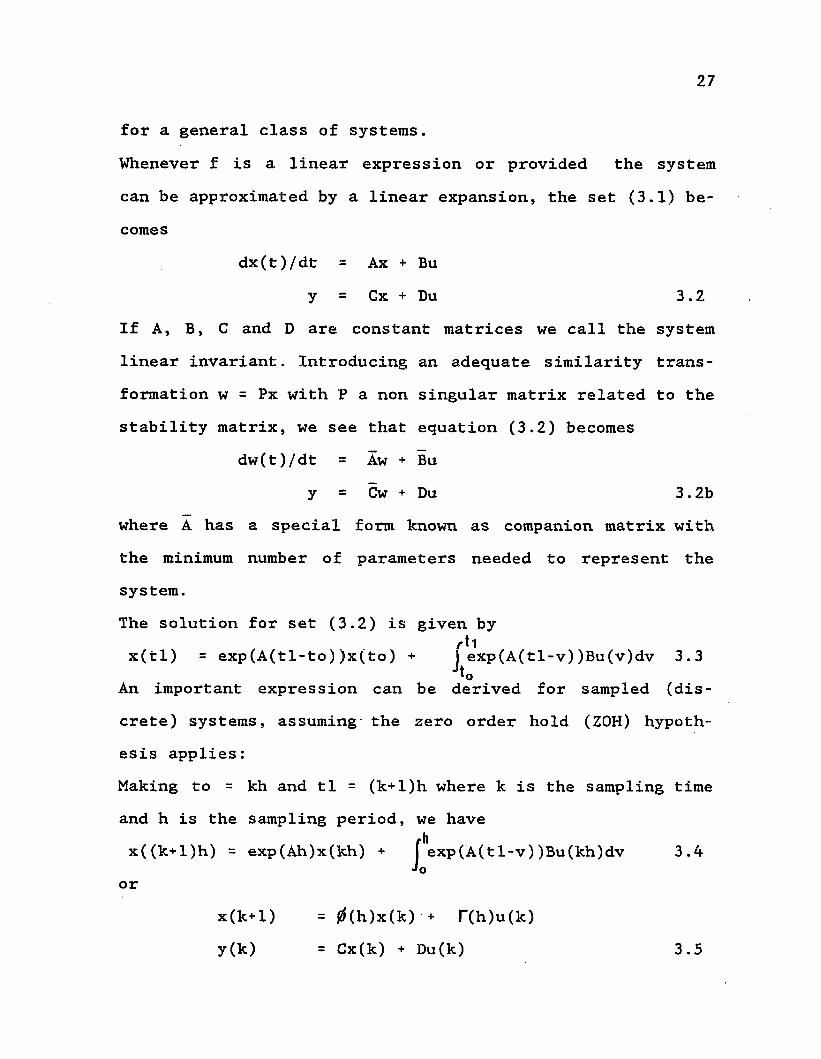
for a general class of systems.Whenever f is a linear expression or provided the system can be approximated by a linear expansion, the set (3.1) be­comes

dx(t)/dt = Ax + Buy = Cx + Du 3.2

If A, B, C and D are constant matrices we call the system linear invariant. Introducing an adequate similarity trans­formation w = Px with P a non singular matrix related to the stability matrix, we see that equation (3.2) becomes

dw(t)/dt = Aw + Buy = Cw + Du 3.2b

where A has a special form known as companion matrix with the minimum number of parameters needed to represent the system.The solution for set (3.2) is given byx(ti) = exp(A(tl-to))x(to) + j exp(A(tl-v))Bu(v)dv 3.3

JtoAn important expression can be derived for sampled (dis­crete) systems, assuming the zero order hold (ZOH) hypoth­esis applies:Making to = kh and tl = (k+l)h where k is the sampling timeand h is the sampling period, we have

/ hx((k+l)h) = exp(Ah)x(kh) + I exp(A(t1-v))Bu(kh)dv 3.4Jo

orx(k+l) = 0(h)x(k) + T(h)u(k)y(k) = Cx(k) + Du(k) 3.5

28

The state space is the most complete representation of a process and contains the maximum amount of information about it.

For a linear, time invariant system, the dynamical be­havior is determined by the eigenvalues of the matrix A.

2.- Transfer Function Matrix representationThis is a mapping of the inputs into outputs relating

the Laplace transform of the vector of outputs with the La­place transform of the vector of inputs. Assuming constant matrices A, B, C and taking the Laplace transform of the ex­pression (3.2) with zero initial state, we have:

(si - A)x(s) = Bu(s)y(s) = Cx(s) + Du(s)

ory(s) = (C(sl - A)"1 B + D)u(s) = G(s)u(s) 3.6

A similar form is derived for the discrete state space equation (3.5) by using the Z transform.

The transfer function matrix contains less information than the state space representation unless no cancellation has occurred. Only the observable and controllable parts of the system are described by the matrix G(s). In spite of lesser information, this method is widely used because the variables that appear are the properties that the operator

29

can measure and manipulate.

3.- Matrix Fraction DescriptionThis is an extension of the single input single output

transfer function and can be derived from the matrix G.Let d(s) be the monic least common denominator of the ele­ments gij(s) of G, then:

G(s) = N(s)/d(s) with N(s) polynomial ma­trix. We can also write

G(s) = N(s)“1(d(s)I) = (d(s)I)"1 N(s) 3.7

and we speak of right and left representations. The matrix fraction is not unique and in general we have:

G(s) = NrDr"1 = Dl“1 Nl 3.8

When the greatest common divisor between (Nr, Dr) or(Nl, Dl)is a unimodular matrix, (Nr, Dr) or (Nl, Dl) aresaid to be coprime. Whenever degree of det(Dr) = degree of det(Dl) = m = order of the matrix A, no cancellation has oc­curred, (Nr, Dr) or (Nl, Dl) are coprime, the system is controllable and observable and, the roots of det(Dr) are the eigenvalues of the matrix A. (Chen (17)).Poles and zeros of G(s)

A polynomial matrix G(s) can always be reduced to its

30

Smith-McMillan form through a sequence of unimodular multiplications. (Patel and Munro (72b)). If the number of inputs n is equal to the number of outputs m then G(s) is equivalent to

M(s) = diag( ai(s)/bi(s)), where ai divides all ai+k and bi divides all bi-k. We define the poles of the system as the roots of all bi(s) = 0 and the transmission zeros of the system as the roots of all ai(s) = 0. Poles and zeros play respectively an important role in the stability of the process and the multivariable system inverse.

3.1.- TOWARD IMC STRUCTUREThe existence of transportation delay in a process has

attracted the interest of controller designers for many years. For conventional analog controllers, the bandwidth and the reset rate are limited to avoid instability with the closed loop system.

Smith (81) proposes a novel method to overcome the problems associated with dead time. Working in a clever way with the block diagrams he first improves the proportional band and reset rate by designing the controller as in a sys­tem without delay. Then he introduces a secondary loop asso­ciated to the controller. The transfer functions G1 and G2 that define the process (except the dead times) appear in this secondary loop in such a way that the final closed loop

31

characteristic equation doesn't contain the dead times. The final block diagram appears in Fig. 3.1

Though the Smith predictor is sensitive to modeling er­rors and is not easy to implement using conventional equip­ment, it is the first successful attempt to modify the controller employing the plant model explicitly.

Joseph and Brosilow (44) design a control system start­ing from a different point of view. Their objective is to infer some process properties from secondary measurements. Doing that, they introduce a model G# in parallel with the plant G to be controlled. The purpose of the model G# is to isolate the effects of the unmeasured disturbances on the process output.

3.2.- PROPERTIES OF IMCLet's represent a controlled multivariable linear process bya conventional feedback block diagram as shown in Fig. 3.2.

_ „ m x n _G C Ra process transfer function matrix C e Ra*m controller transfer function matrixy e R output vectoru e Rn control vectord e Rm disturbance vector

Ra is a commutative ring of rational stable functions with real coefficients.Ra is a noncommutative ring whose elements are (mxn) ma­trices with elements belonging to Ra.

^ 9 - V .e,e-Tis Mo- 82e -T2s

■ , ¥ F = (I - e'^i+T2^s)

Fig. 3.1 Smith Predictor

sp

Fig. 3.2 Common Feedback Loop

33

R is the field of real numbers and R n is the n-dimensional vector space defined on R.The system matrices and vectors are implicitly functions of a general variable p that represents the Laplace variable s for continuous processes and the z variable if the system is discrete.The output y is easily calculated as

y (p) = G(I + CG)"1 C(sp-d) + d 3.9Defining perfect control as:

y(p) = sp(p) any d and any time; 3.10we can conclude that perfect feedback control is achievable if and only if |C|— > oo (whatever definition of norm we use).From the block diagram

u (p) = C(I + GC)"1 (sp-d)and

Gu = GC(I + GC)"1 (sp-d)

for perfect control Gu = y-d = sp-d therefore

GC(I + GC)"1 = I 3.13and this requires that the right inverse of G exits. The ma­trix G has a right inverse if and only if rank of G = m so,

3.11

3.12

34

the number of manipulated variables n must be at least equal to the number of outputs m. The Moore Penrose generalized inverse must be understood if n > m.

The configurations developed by Smith and Joseph and Brosilow, were adopted by Garcia and Morari (31), under the structure shown in Fig. 3.3.The model G# appears in parallel with the plant and with the controller. After replacing the dashed block by its algebra­ic equivalent, we obtain the final internal model control structure as shown in Fig. 3.4.The following equivalences hold:

Gc = (I + CG#)”1C or

C = Gc(I - G#Gc)"1 3.14

No specific form is required on C except the conformability of the matrix products. Furthermore, the block diagram in Fig. 3.4 is algebraically equivalent to the conventional feedback control in Fig. 3.1.After some manipulations, the output y is expressed by:

y(p) = G(I + Gc(G - G#))“1Gc(sp-d) + d 3.15

From this, the well known properties of IMC structure fol­lows. (Garcia and Morari (31)).

35

Fig. 3.3 Parallel Model Structure

Fig. 3.4 Internal Model Control

36

1.- Perfect modeling;if G# = G

y = GGc(sp-d) + d 3.16

then, the stability of the closed loop will be assured if G is open loop stable and Gc is chosen also stable.2.- Perfect control;If Gc is chosen as the right inverse of G in (3.16) then perfect control is achieved. (At least in theory). The need for the right inverse of G follows na­turally in this approach and is equivalent to equations (3.13) and (3.14).3.- Asymptotic perfect control;zero offset is asymptotically obtained if Gc is chosen such that:

lim Gc(p) = ( G#(p*))~1 3.17p — > p*

where

i O if p = s, continuous systems

1 if p = z, discrete systemsMaking the controller Gc equal to G inverse is seldom possi­ble. Several problems arise related to inherent properties of the plant itself.1.- Non causal inverse. Whenever some delay is present in the plant, its inverse leads to non realizable functions.2.- Nonstable inverse. If G has transmission zeros in a non-

37

desirable zone (lambda zone), then its inverse will be un­stable. The lambda zone is defined by extension of the con­ventional RHP subset of the s-plane, or, for discrete systems,as the region outside the circle |z| = 1. The de­signer usually defines the lambda zone according to some particular criterion. (For example, to avoid oscillation).3.- Improper inverse. Even when dealing with causal and sta­ble inverses, strictly proper process models will lead to improper inverses that present extreme sensitivity to high frequency perturbations.The construction of the control function must consider all these problems. Usually, the transfer function G# is repres­ented in the form of a product of two factors:

G# = G+ G- 3.18

where G+ contains all the non invertible properties of G#and G- is called the lambda invertible part of G#. (The plus is adopted by analogy to the unstable positive semiplane s. In the book of Astrom (12) for example, the converse is as­sumed) .The controller is then expressed as:

Gc = (G#)“1G+F 3.19

The term F corresponds to a filter function that compensates

38

the improper form GT* .G+ is not unique and several techniques have been developed to construct it.Under perfect modeling, the output y(p) becomes:

y = G(G#)"1 GtF(sp-d) + d or

y = G+F(sp-d) + d 3.20

The difficulties associated with the plant structure appear explicitly represented by the factor G+ . For example, if the plant has a delay, exp(-Ts), the setpoint tracking or the disturbance rejection can be achieved only after a time T has elapsed, these features are included in the term G+. in (3.20).

3.3.- ROBUST DESIGNThe preceding discussion about the controller design

was done assuming perfect modeling of the plant. Under un­certain models, equation (3.15) can be modified introduc­ing explicitly the filter F. The first condition for sta­bility follows immediately:

det (I + GcF(G-G#)) y* 0 3.21

for any value of the generalized variable p and for any G#

39

that can represent the plant.Manousiouthaki et al (60) define a topology over the

set of all possible variations of G with :E(G, 6 ) = (G'eRaXn (p) s.t. g ’ij E(gij, 6ij) V i=l, 2 .....m, V j=l, 2, n) and a similar topology is defined forthe scalar transfer function gijE(gij , dij) = (g’eRa(p) s.t. | g f ij-gij | po< 6ij (w) ^ pos 6A). 6Ais the boundary of A and dij(w) = max|gij(po)-g'ij(po) | ,V" po c 6 A .

A norm definition for matrices is necessary. The spec­tral norm, based on the maximum singular value of the ma­trix, is adequate for this purpose. (See Arkun et al (8)).

To achieve asymptotic perfect tracking, the closed loop transfer matrix must accomplish:

G(p*)Gc(p*)(I+F(p*)(G(p*)-G#(p*))Gc(p*))“1F(p*) = I 3.22

applying (3.17) and after some manipulations

F(p*) = I for any plant variation 3.23

The stability condition requires that the roots of the expression det (I+F(G-G#)Gc) must never encircle p* and therefore, the determinant must never change sign as the plant varies over E(G, 6 )• When G is equal to the nominal plant G#, the determinant becomes one. This fact fixes the

40

sign for all the allowable variations of G and therefore :

det (I+F(G-G#)Gc) > 0 3.24

for any G over E(G, ) and any p.If p 5 p*, (3.17), (3.23) and (3.24) imply :

det (G(p*) G#(p*)~1 ) > 0 3.25

so, the changes in the plant G with respect to a nominal model G# cannot be such that restriction (3.25) is broken.

Levien and Morari (57) present a distillation column’ model and show how the change of three parameters in a (3x3) system leads to instability. (Though the changes are rather excessive :100%).Disturbance rejection and Filter DesignThe control vector is found directly from Fig.3.2:

u = Gc(sp-d) 3.26

If G# can be factorized into a lambda invertible matrix G-and a non invertible part G+ such that IG+I = 1 then Gc isconstructed as:

Gc = G-1 F = (G#)“1 G+ F 3.27

Therefore, replacing the last expression into (3.26)

41

u = G-1 F(sp-d) = (G#)-1 G+- F(sp-d)

we see that the norm of u is given by:

|u| = | (G#)-1 ||sp-d| < |u|max and

|sp-d| < |G#||u|max

For a regulator problem, the magnitude of the disturb­ance is bounded by the norm of G#. This norm can be repres­ented by the greatest singular value of G#

| sp-d| < tJj| (G#)|u|max 3.28

At high frequency, (G#) is small and the magnitude of the allowable disturbance is also small due to the saturation of the control vector u.

Zafiriou and Morari (95) use the singular value ap­proach to design an optimal filter. They recommend a simple diagonal structure for F to keep the number of variables small at the optimization stage. Nevertheless, the algorithm requires the calculation of gradients and it is rather com­plex.

Kantor (46, 447 using the spectral radius instead ofthe singular values, proposes another filter design method under internal model control structure.

CHAPTER IV

MODELS AND ESTIMATION

4.1.-MODELSA model is a representation of a reality that we pre­

tend to know. There are many levels of modeling, several ways to proceed with them and a given phenomenon usually has associated with it more than one model.

In a first level, we can consider some physical scaled representation of the actual system. For example, architects build small scale models of houses and with them they are able to study the best orientation of the house with respect to hours of light, relationship with the landscape etc.

In a second level, more advanced applications are sought and our purpose is to use the model to describe re­lationships among the different properties of the process. The set of equations that describes such relationships is called the mathematical model.

A model may change and normally the modifications are suggested by the knowledge we get from the previous ideas. A beautiful example of model evolution is given by the struc­ture of the hydrogen atom. First, it is thought of as a solid sphere. Some gas kinetic properties are studied using this primeval model but, it is impossible to predict from it other properties of matter. The next approximation considers

42

43

the atom as a nucleus with an orbiting electron. More infor­mation is gained but some phenomena are still left without explanation. A third stage considers the electron orbit as a probability density and a dual wave-particle behavior for the electron. Again, more knowledge is obtained. Of course, we pay for the advances with more complex mathematics, so it is necessary to establish a trade off between investment and return.

Generally, the starting point for building a model is a set of relationships known as conservation principles.

Mathematically we talk of static or dynamical models, continuous or discrete , deterministic or stochastic etc.

We must never pretend that a model is the real life ac­tual system. In fact, our models have a more pragmatic sense and their acceptance is guided by their usefulness, that is, we are normally more concerned whether the model can fit experimental data than with philosophical aspects of the representation of reality.

Sometimes, specially when testing a given identifica­tion procedure, we compare the results with those obtained by simulation of the "true" plant. Of course, this ex­pression must be understood in a figurative sense since the "true" plant is nothing more than a higher level model used to generate some data such as a real plant would provide.

44

Input-output models.The properties associated with a system are called var­

iables and are classified as inputs and state variables. Those properties that exist independent of the system itself are called inputs. The properties that are a consequence of the inputs and the modifications introduced by the plant are called state variables. Some of these state variables or combinations of them that have an external manifestation are called outputs. From the mathematical point of view, all the inputs are equivalent but, according to engineering charac­teristics, such as our ability to handle them, they are classified into perturbations and control variables*. In this way, the steam flow to a process and the environment temper­ature are both inputs, but it is much more comfortable to think of the steam as an operative variable and to treat the temperature as a perturbation over which no possible control action can be exerted.

Computer oriented modelA fundamental problem is how to describe a continuous

system connected to a digital computer. The discrete opera­tion of the computer requires that the continuous flow of information from the plant be converted to a sequence of numbers that the computer can process. The signals are sent to the computer through an analog-to digital converter and returned to the plant with a digital-to-analog device.

45

O C E S S

C O M P U T E R

Fig.4.1 Digital Control

The symbols ( u(k)), (y(k)) mean sequences of numbers corre­sponding to the values of u(t) and y(t) at the sampling time k At- An internal clock decides when the sampling must be done.

4.2.-IDENTIFICATIONSystem identification is the construction of models

starting from input-output data for a given plant. Identifi­cation is important to theory but it also plays a valuable role in the design of control systems and can be considered as the experimental building of models.

The identification stage is an open problem with se­veral degrees of freedom. This freedom can be bounded ac­cording to our knowledge of the process to be identified. The black box approach assumes we know nothing about the system, but of course this is a very restrictive way. Usu­

46

ally, the previous knowledge about the process is signif­icant, and we have approximate ideas of its performance with different kinds of stimuli, relative magnitude of response, dead time in the response, presence of non-linear effects like Arrhenius's expression etc.

The complete identification problem requires the deter­mination of a structure and the related parameters. The task is made easier if we assume a model structure (for example, a transfer function matrix), and we just calculate the asso­ciated parameters. In that case, we have reduced the iden­tification problem to one of parameter estimation.

Astrom (12) points out the following features to help with identification:

Experimental planningSelection of model characteristicsEstimationValidation

4.2.1.-Experiment designTo design an experiment leading to the identification

of a plant, we need to solve several questions such as what and when to measure, how many measurements, what kind of in­puts etc. Many of these questions will have an appropriate answer only after the plant has been identified. As usual, some design decisions must be taken without sufficient in­

47

formation. Of course, previous knowledge of the plant and skilled operators will be a worthy help. On the other hand, restrictions do exist;some of the variables are very diffi­cult or impossible to measure (catalytic activity for exam­ple), some instruments are too expensive others too slow etc. Furthermore, too much information can be confusing and difficult to process.

With respect to inputs, our main concern should be to reduce the perturbations to the minimum amount. If possible, the normal operating values must be used. Whenever addi­tional inputs are required, the excitation must be persist­ent, that is, rich in information. Appropriate inputs for identification purposes are pseudo random binary sequences (PRBS) and white noise signals. The amplitude of the signals must be selected specifically for each system. In the same way, the period of the binary sequence must be chosen ac­cording to the dominant time constant. To improve the esti­mation, it is desirable to use normalized input-output pairs.Sampling period.

The selection of the sampling period h is of paramount importance; and unfortunately, linked with the unknown dy­namics of the system. It would appear, as a first guess, that h should be chosen very small to have a better repre­sentation of continuous signals, but this would mean a great increase in the computer load. Even worse, if the process is

48

slow, a large sampling frequency means an ill conditioned information matrix with the subsequent inversion problems. Astrom (12), recommends the choice of 1/h six to ten times the bandwidth of the closed loop or two to three per rise time. Sometimes, multirate sampling is introduced to avoid the use of complicated antialiasing filters. This is spe­cially convenient for multivariable systems where one of the variables is slow relative to the others. If the sampling periods are synchronized and hi = nh2 with n integer, then the ordinary theory for discrete systems can be applied.

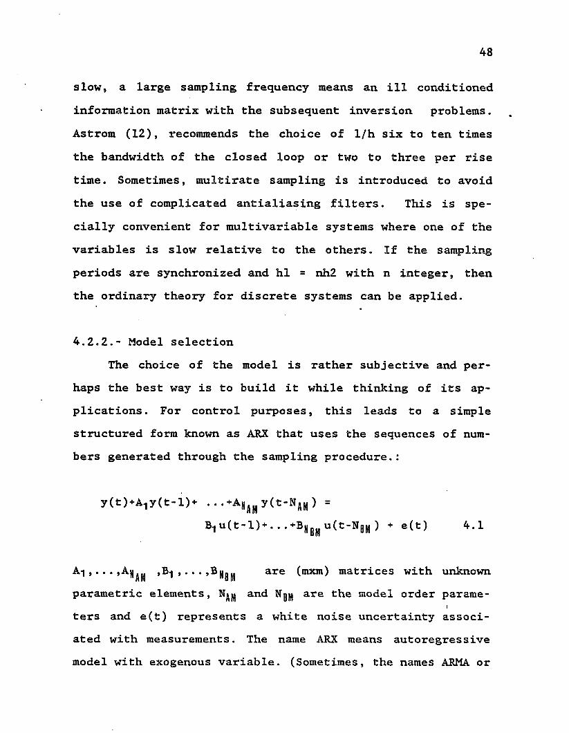
4.2.2.- Model selectionThe choice of the model is rather subjective and per­

haps the best way is to build it while thinking of its ap­plications . For control purposes, this leads to a simple structured form known as ARX that uses the sequences of num­bers generated through the sampling procedure.:

y(t)+A1y(t-l)+ . . .+A(|flM y(t-N flH ) =B1u(t-l)+...+BN u(t-NBM) + e(t) 4.1

A i ,. . . »A)|^ ,B-j ,. . . ,Bjjg are (mxm) matrices with unknown parametric elements, and Ngjj are the model order parame-

Iters and e(t) represents a white noise uncertainty associ­ated with measurements. The name ARX means autoregressive model with exogenous variable. (Sometimes, the names ARMA or

49

DARMA are also used).After introducing the shifting operator q such that

q-1f(t) = f(t-l) 4.2

equation (4.1) becomes

(I+A^"1 +. . .+AN q-NflH )y = ( B ^ - U . . .+Bj,BM q-NBH )u + e 4.3

We define the polynomials matrices:

A(q) = I + A1q“1 + ...+ A NftHq~NftnB (q) = 6^-1 + . . .+ BN|JH q-NBH

then equation (4.3) becomes

A(q)y = B(q)u ■+ e 4.4

solving for y we introduce the transfer matrices:

y(k) = A"1Bu(k) + A“1e(k) = G#(0, q)u(k)+ He(k)

According to the system complexity (and our knowledgeof it), more sophisticated expressions, such as non-linear effects, can be introduced. Once the structure of the system has been adopted, the order and Ngm must be chosen. Ljung

50

(59) propose several methods to test the order, but most of them are highly complex using spectral analysis of G# or the rank of the information matrix. A more pragmatic approach consists in the comparison of performances for two models with a fresh data set (cross validation). Another practical way is the minimization of the loss function with respect to the order. Some care must be taken to avoid overfit and therefore overparametrization.

4.2.3.- Estimation algorithmOur main interest is directed to adaptive control and

therefore, to on-line, recursive algorithms. Goodwin and Sin (37) present complete information about the available meth­ods .

For use on-line, we need a simple and fast algorithm and the recursive least square seems to accomplish these re­quirements. Note that recursive least square is intended for linear estimation but, the linearity is referred to the parameters and not to the system itself. Agarwal and Seborg (1, 2) present a good example of a non-linear adaptive con­trol for single and multiple variable systems.

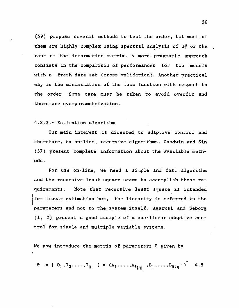
We now introduce the matrix of parameters 0 given byI

0 - ( 0-j ,©2» • • ■ >® |d ) — ( 1 j • • • ’ Nuid ’ * * ■ * ’®Ng|d 4.5

51

where 91 are NPxl vectors, Ai and Bi are mxra matrices and NP

= NAM + n bh ■At each step N, the vector 0i(t) is determined as function of the last estimation 9i(t-l) and a gain vector K(t) inC11 pVi a Mfliv fft m*i m ’ m i t-Vio 1 n C o -Pi inr*f*n •w m v * * %• n w j w su w w t A W a v w w i> j. •

N TJ(9) = ( I e'Ke J / N

eK = yK- yK 4.6

Upon defining the regressor 0 as :

0 T = (yT(t-1),...,yT(t-NAM),uT(t-1),...,uT(t-NBH)) 4.7

the following recursive algorithm results:

9i(t) = 0i(t-1) + K(t-l)(yi(t)-0T(t-1)0i(t-1)) 4.8

K(t-l) = P(t-l)0(t-l)(1 + 0 T(t-l)P(t-l)0(t-l))”1 4.9

P(t) = P(t-l)-K(t-l)(l+j3T(t-l)P(t-l)pT(t-l))KT (t-1) 4.10

This multivariable estimation algorithm follows Borison’s presentation (15) and the proof of minimization can be found in Goodwin and Sin (37).Some modifications can be done to improve the character­

52

istics of the algorithm. To cope with time varying systems, it is necessary to eliminate or at least to attenuate the weight of the old data. This is done by introducing a for­getting factor in the loss function:

N u kJ(9) = I A" K (y(k)- 9(k)0(k))**2/N1

The value of A is less than one and appears in the updating of P and K.

K(t-l) = P(t-l)0(t-l)(A + 0 T(t-l)P(t-l)0(t-l)) 4.11

P(t) = (I - K(t-l)0T(t-l))P(t-l)/A 4.12

with initial estimation

9(0) = 0, P(0) = al ; a > 106

The forgetting factor presents some problems when the system has been running steadily and, the input data are no longer persistently exciting and P grows exponentially. If some sudden change occurs under this condition, the esti­mation algorithm is highly sensitive and the controlled sys­tem becomes unstable unless some detuning is applied. This phenomenon has been studied by several authors and one of the best approaches is due to Fortescue (29). Based on the

53

information content of the data, he develops a procedure to make the forgetting factor variable, with a value very near one when the estimation has converged. If some change is de­tected, the forgetting factor decreases and the estimator is reactivated.

Astrom (12) proposes a very simple algorithm to achieve a variable forgetting factor:

A = 1 - p e ^

where e is the prediction error, e is the mean value over agiven period of estimation and p is a constant factor

We use e2 = (1+0^(t-l)P(t-l)0(t-l)) (Goodwin and Sin)

then A = 1 - p e2 / (1+0 "P0) which is basicallyFortescue's algorithm.

Covariance matrix factorizationFrom a numerical point of view, the information matrix

P can be very ill-conditioned specially for large systems. The convergence of the estimation is related to the condi­tion number Y defined by:

Y= pmax P(0)"1 / pmin P(0)"1 with p eigenvalue of P sothat if Y is closer to one the convergence is improved and

54

| e ( t ) - 0 o I < | 0 ( 0 ) - 9o |

where © is the current estimation matrix, 0o is the true ma­trix of parameters and 9(0) is the initial estimation ma­trix; To improve the performance, Bierman and Thornton (14), factorize P as the product of three matrices:

P = U D where D is a diagonal matrix and Uis upper triangular. Another approach is to consider the Cholesky decomposition or any other method that allows to express P as the product QQ^ . The loss function is not affected by the transformation but, the ratio between the largest and smallest eigenvalues of Q is the square root of that of P and therefore, the new system will be better con­ditioned than the original. Peterka (76) presents an algo­rithm called REFIL written in such a way that it can be directly implemented in a computer program. This program, with the variable forgetting factor introduced by Fortescue was the workhorse in all our estimations Remarks.1.- No information in advance is required for the delays of the system. It is advisable however to make a rough esti­mation to fix Ngm .2.- The same algorithm REFIL can be used for extended least square or non-linear systems by changing the way in which the regressor vector 0 is constructed.

55

4.2.4.- Model validationOnce the model structure has been fixed, the order has

been selected and the parameters calculated, the natural questions that arise are:Does the model fit the data?Is it simple enough for control purposes?How easy (or not) is it for the computer to estimate the pa­rameters?There are also other questions concerning the philosophical approaches to the true plant, but from a practical point of view they are less relevant than the former.

For linear systems a well known practice to evaluate different models is through the comparison of Bode plots, but this approach is not appropriate for multivariable proc­esses .

With a fixed structure, only two degrees of freedom are left: Num and Nnjj . To answer those questions, we looked for the minimum values for these parameters that allowed a rea­sonable fit. The practice was to start with = Ng^ = 1,increasing Ng^ we looked for the minimum of the loss func­tion

Ns oJ = Z (y-y#) /Ns.1

Then, was incremented by one and the procedure was re­peated.

56

The cross validation resulted in a very good tool that is self-implemented in a process with internal model con­trol. The crucial part of IMC is to work in an open loop form, that is, with perfect modeling. First the model was estimated using some persistent excitation and then, the fresh data was entered through changes in the reference vec­tor. The difference (G-G#)u is then, the best index of how well the model behaves.

CHAPTER V

FACTORIZATION AND INVERSION

IntroductionFor linear systems perfect internal model control re­

quires the inversion of the plant model represented by the transfer function matrix G#. As discussed in chapter three, this inversion is seldom possible and therefore, an approxi­mate inverse is sought after the matrix G# has been factored into a lambda-invert ibid part G- and a non invertible term G+ .

We are concerned with rational proper functions G# but, due to the nature of the ARX model explained in chapter four and to the estimation algorithm, the matrix G# is already expressed as the product of two polynomial matrices:

where A and B are defined in (4.3) and correspond to the partitioned matrix 0 defined in (4.5).

G# = A"1 (z-1 )B(z-1 ) 5.1

e (01>©2 e||) = (Ai. . . . ,An ,Bi, . . . ,B||bh )T 5.2

From (5.1):

57

58

(G#)-1 = B-1 (z-1 )A(z-1 ) 5.3

Expression (5.3) must be considered as a formal one because we still do not know under what conditions the inverse of matrix B exists.

Hereafterj the argument z corresponding to discrete systems will be used since it is the natural way for itera­tive estimation. Nevertheless, the development that follows is general and can be applied to continuous systems.

Expression (5.3) points out that the factorization and inversion problem is reduced from working with rational ma­trices to handling polynomial matrices. Therefore, the best linear control under IMC structure will be defined as long as we are able to obtain the factoring and inversion of the polynomial matrix B.

5.1.- MATRIX FACTORIZATIONBy factoring a polynomial matrix B(z) we must under­

stand the search for two new polynomial matrices B+(z) and B- (z) such that they have their zeroes in disjoint sets of the complex plane. Normally the A region (region of B+ zeroes) is defined as the set of all points in the extended plane C+, such that these points have given properties. As a first step, lambda contains the unstable poles such as the points inside the unit circle, but it can be enlarged to other points that the designer does not want as poles. By exten-

59

sion we call a matrix lambda-stable if its poles are out­side the lambda zone, though not necessarily all points in­side lambda are unstable. Such factorization is always possible under very mild conditions (e.g., the matrix must be analytic) and is closely related to the minimal realiza­tion problem. (Bart et al.(13)).

5.1.1.- Transmission zeroes and poles of a matrixThe definition of the lambda-region is based on the

stability properties of linear systems and therefore, on the concept of zeroes and poles of multivariable systems.

For a given matrix G with elements gjj , scalar rational transfer functions, we define the transmission zero p as a value of z such that it reduces the column rank of G. That is, if p is a transmission zero of G, there exists a non zero vector b such that:

G ( p ) b

(b is called a latent vector of G )The definition of pole is not so expeditious and there­

fore we must first define the Smith-McMillan form of G.Let d be the monic least common denominator of all g. ,e»ij >

then:

G(z"1 ) = N(z-1 )/d(z~1 ) 5.4

60

where N(z"1 ) is a polynomial matrix, we define:

a) fo = 1b) fi = the monic largest common factor of all

(ixi) minors of N(z “1).c) QJi = fi/fi-1Then, the diagonal matrix S

S = diag( ipi) 5.5

is called the Smith form of the matrix N and can be obtained from N through a finite number of transformations.Finally, dividing by d(z“1 ) we have:

M(z“ ) = S/d(z"^) = diag(ai (z_1 )/bi (z-1 )) 5.6

M is called the Smith-McMillan form of G. From M, the poles of G are defined as the roots of the polynomials bi(z-l). Thus, the A-zone is defined as the collection of points in the complex plane that the designer doesn't want as roots of bi(z-1 ). For example, for a discrete system we may define lambda such as:( z c A / z s . t . |z| >0.8)

Note that the A-zone includes stable points.

61

Once the A-zone is defined and the Smith-McMillan form of G has been obtained, the factorization of any matrix is rather trivial. The difficulty is hidden in the search for the Smith form. Although this is an elementary procedure, the numerical methods are unsatisfactory.

Kontos (50), uses an alternative form based on the ele­mentary factors of the polynomial matrix and on its latent vectors. Unfortunately, the determination of latent vectors requires the singular value decomposition of the matrix for each of its transmission zeroes and therefore the method is not appropriate for on-line implementation.

5.2.- MATRIX INVERSION AND FACTORIZATIONSo far, no available factorization algorithm seems to

be appropriate for on-line calculation.The following scheme was developed for obtaining an al­

gorithm that reduces the matrix factorization to that of a scalar polynomial and that is appropriate for working on-line.

From (5.6) we can see that the zeroes of the matrix G, that will be the poles of an eventual inverse matrix, appear in the diagonal of the Smith-McMillan form of G and there­fore their product is contained in the determinant of G. This leads to solving first the inversion problem. The fac­torization will then result as a consequence of the inver­sion procedure.

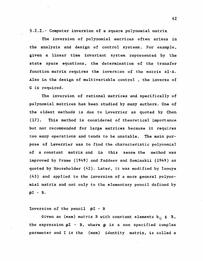
62

5.2.2.- Computer inversion of a square polynomial matrixThe inversion of polynomial matrices often arises in

the analysis and design of control systems. For example, given a linear time invariant system represented by the state space equations, the determination of the transfer function matrix requires the inversion of the matrix sI-A. Also in the design of multivariable control , the inverse of G is required.

The inversion of rational matrices and specifically of polynomial matrices has been studied by many authors. One of the oldest methods is due to Leverrier as quoted by Chen (17). This method is considered of theoretical importance but not recommended for large matrices because it requires too many operations and tends to be unstable. The main pur­pose of Leverrier was to find the characteristic polynomial of a constant matrix and in this sense the method was improved by Frame (1949) and Faddeev and Sominskii (1949) as quoted by Householder (42). Later, it was modified by Inouye (43) and applied to the inversion of a more general polyno­mial matrix and not only to the elementary pencil defined by pi - B.

Inversion of the pencil pi - BGiven an (mxm) matrix B with constant elements bjj e R,

the expression pi - B, where p is a non specified complex parameter and I is the (mxm) identity matrix, is called a

63

pencil of matrices.It can be shown that:

(pI-B)“1 = (R0pm “1 +R1p m“2 +...+ R m_2 P + R m-,)/A(p)

where A(p) = det(pI-B) = p m +aiPm~1+. . . . + a m

with aj and Rj constant scalars and matrices respectively and defined by:

°1 = -trBR0 /I R„ = Ia2 = -trBR-j /2 R-| = BR0 + a11a3 = -trBR2 /3 R2 = BR1 + d2I

• • • • • • am = - trBRm_ -j/m 0 = BR m-1 + amI

where tr stands for trace of the matrix. In other words, the algorithm allows us to express the inverse of the elementary pencil as:

( p l - B ) “ 1 = a d j ( p l - B ) / A ( p ) 5 . 7

•

providing an iterative method to compute <Jj and Rj .After using the fact that the inverse of any (mxm)

monic polynomial matrix B with degree n

B = B q +B-jP + ... + Ipn 5.8

64

can be expressed in term of an elementary pencil of matri­ces, Inouye (43) modified the method of Leverrier producing a fast and reliable algorithm that reduces the inversion to handling (mxm) matrices.Two problems remain :

1)The method is not completely general because theleading matrix B n must be the identity matrix or at leastnon singular.

2)The algorithm is valid only with column (row) reduced matrices, that is deg det(B) = Z 6 c j B(p)

where 6ci B is the highest power of p in all the elements ofcolumn i. Now, any non reduced matrix can be reduced through the multiplication of unimodular matrices but the condition is not easy to test and the search for the unimodular matri­ces is complex and not appropriate for on-line computation.Buslowicz (16) established an algorithm that improves Inouye's method making it less restrictive and faster. Buslowicz algorithm:Given B(p) = Bo +B.j p + ... + Bnp n ; Bi (mxm);then: 5.9

detB(p) = a„ + a1p + ... + arpr 5.10with r less than or equal to mn Therefore:

■« n m - n ,B(p) = Z Qkp /det(B) = Q/det(B) = adj(B)/det(B) 5.11 o

with

65

Qk = (-l)m+1 Rm -1 ,k ; k = 0,1, . ..,n(m-l)ak =((-l)m+1tr Gm,k )/m ; k = 0,1,..,mn

II if k = 0

.■

0 if k * 0 Rj,k = Gj,k + aj,k*I ; j = 1,2, ...,m-lRm, k = Gm, k + am, k*I ; k = 0,1, ...,mnGi,k = BoRi- ,k+BlRi- ,k-l+ ... + BnRi- ,k-nai,k = (-tr Gi,k)/i ; i = 1,2, . . . ,m

set 5.12Even though this algorithm is more complex than that of

Inouye, it was implemented as a computer program called POLIN (POLynomial INverse) using FORTRAN 77.(See appendix B). The program worked efficiently under test conditions and also on-line integrated to the IMC controller. In the tests it showed that it is fast, reliable and free of numerical problems even when B is a very ill-conditioned ma­trix, because the adjoint of B always exists independent of the values of det(B).

Note that in the algorithm the augmented matrices have been replaced by an increased number of (mxm) matrices.

Factorization of the inverse of BOur conjecture is that all the required dynamical in­

formation is contained in det(B). At this point we return to the variable z “1 specific for discrete systems. All the in­

66

version steps are valid if we replace p by z-1. Solving nu­merically for det(B) = 0, det(B) can be separated into three dynamical factors and a constant.

det(B) = a0 + a-jz” + ... + a^z“N = z"N0 A* (z-1) A“(z~1 )a^ 5.13

ND represents the non-causal factor due to dead time. A* (z ) contains the unstable part of B (roots E A ), A" ( z ) is the lambda stable factor of B (roots outside A) and, a. is the coefficient of the highest power of z“1 in the determi­nant polynomial. This last factor is taken out to produce monic polynomials A* and A~ .

We define the following parameters according to the factori­zation:

ND : global dead time of the processN + : number of A-roots of det(B)N_ : number of stable roots of det(B)N : total number of roots of det(B)

The above parameters have an internal meaning and were cal­culated at each iteration.Let's illustrate the procedure with an example.Assume A (z“1) = 6z_3+ 39.8z_4+74.4z~5+58.4z-6

20.4z-7+2.6z-a such as would be provided by the inversion program.

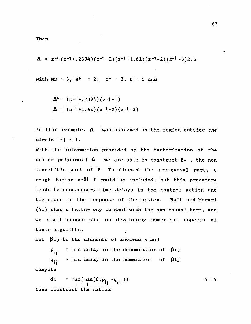
Then

A = z - 3 ( z - 1 + . 2 3 9 4 ) ( z - 1 - l ) ( z “ 1 + i . 6 l ) ( z - 1 - 2 ) ( z - 1 - 3 ) 2 . 6

with ND = 3, N+ =2, N“ = 3, N = 5 and

A + = ( z - 1 + . 2 3 9 4 ) ( z - 1 - 1 )

A " = ( z - 1 + l . 6 l ) ( z - 1 - 2 ) ( z - 1 - 3 )

In this example, A was assigned as the region outside the circle | z | = 1 .

With the information provided by the factorization of the scalar polynomial A we are able to construct B+ , the non invertible part of B. To discard the non-causal part, a rough factor z-HO I could be included, but this procedure leads to unnecessary time delays in the control action and therefore in the response of the system. Holt and Morari (41) show a better way to deal with the non-causal term, and we shall concentrate on developing numerical aspects of their algorithm.Let Pij be the elements of inverse B and

p.. = min delay in the denominator of (3ijq.. = min delay in the numerator of 3ij

Computedi = max(max(0,p.. -q., )) 5.14j j 'I i!

then construct the matrix

68

D = diag(z”di)

The matrix D deals with the non-causal terms of B in a de­coupled way. This decoupling is optimum in the sense that D provides the minimum amount of delay to each row in such a way as to cancel out the non-causal term z~N0 . If the most relevant dead times are not in the diagonal of B, the can­cellation is not optimal but the decoupling characteristics are maintained.

According to the way in which B" is calculated, adjB is a new polynomial matrix therefore, p.. = ND for all i, j andwe only have to compute and thus the calculation of diis almost inmediate.Finally B+ was constructed in the following form:

A + ( z ~ 1 )B+ = ----------- diag(z-dj ) 5.15

A+U)

Therefore, the stable and causal inverse of B is :

adj(B)BI1 = B_1 B+ = ------------------------ diag(z~di ) 5.16

z - H D A - ( Z - 1 ) A + ( 1 ) a | |

orQN

B- = ----------------------- 5.17A” (z~ ) A+ (1) a ||

where QN is the matrix that results after multiplying adj(B) by matrix D and cancelling z ~ N D .

69

The factor A + ( 1 ) is included in ( 5 . 1 5 ) so that B+ ( 1 ) = I and therefore BI^ (1) becomes exactly B"1 (1) when time goes to infinity.

5.3.- SYNTHESIS OF Gc.Once the approximate inverse of B was constructed, the

implementation of the control algorithm followed from ex­pression (5.3).

Gc = (G#)"1 F = B-1 AF 5.18

F is a diagonal matrix filter included to make the control action robust. For simplicity's sake, the filter was defined as a first order lag with elements f- = (1- Qj)/(1- dj z~1 ) with aj tunable parameters.Introducing expression (5.17) into expression (5.18)

QN A F H FGc(z ) = ----- -------------- = ---------------- 5.19

A " ( z - 1 ) A + ( l ) a A " ( z - 1 ) A + ( 1 ) a „

The control vector was calculated as:H F 8

u = Gc(sp-d) = Gc 8 = 5.20A - ( z - 1 ) A + ( l ) a N

The difference sp-d = 8 is the generalized error in the IMC structure.Making F8 = x, Hx = v, we have:

u ( k ) = ( v ( k ) / ( a H A + ( l ) ) - X b j u ( k - i + l ) ) / h , 5 . 2 12

70

w i t h b j c o e f f i c i e n t s o f t h e s t a b l e p o l y n o m i a l A " ( z - 1 ) .

Thus, u(k) was generated as a function of present and past generalized errors and past inputs.We can summarize this chapter by stating that a method for inverting and factoring a polynomial matrix B was success­fully developed. The algorithm is based on the properties of the Smith-McMillan form of B but without searching for it. The method starts by inverting the matrix and then the matrix factorization is reduced to a scalar problem appro­priate to be solved on line.A complete example of the procedure is presented below

The following discrete model was used for representing a continuous distillation column:

n am = 1» n bh= 3 ’ m = 2

At arbitrary time = 64, the estimated parameters are:

‘1. o. ■ '- .921 -.022'A = +

.0- 1.. .-.223 -.747.

' .717 -.016' z -1 + ' .005 0.004" ‘-.005 -.856’B = z"2 +

- .353 .517 1.076 -1.017. .-.734 -1.235.

The matrix B is then submitted to the inversion algorithm POLIN. The following information is returned:

71

det(B)=(.3653-.7088z-1 -1.2109z~2 +.9253z~3 -.6262z“4)z-2

'.517 .016" '-1.017 -0.004' '-1.235 .856'adjB= z-1 + Z "2 +

..353 .717. .-1.076 .005. . .734 -.005

Det(B) is then factored into a stable factor and a non-cau- sal unstable part using Mullers method plus an ordering al­gorithm.Therefore:

z"2a + = (z“1 -.3494)(z“1 +.6305)z“2 A" = (z-2-1. 7587z'1 +2.7203)(-.6262)

with ND = 2This factorization is specific for ( z e A / s.t. |z| < 1). If a different definition of A is used some of the roots will move from A ” into A + .The terms q^ are calculated from the elements 3ij of the matrix adj(B):

pij = p°ij +p1ijz-1 + ... + p rijz~rand

q.. = K with K the first term such thatIJ

IP K ij| > 10“n*max(|p 1 ij|) 5.22L

With this criterion we are neglecting parameters that are10"n times less than the maximum coefficient. A value for n

72

equal 2 or 3 was found appropriate.In the example, one element of adj(B) is:

3 11 = .5l7z-1 - 1.017z-2 -1.235z-3 and therefore

max(IP1111) = 1.235L 1

for n = 3, 3 11 fits the criterion and so K - 1 ==> qll = 1 From this dl and d2 are calculated:

dl = max(max(0, ND-qll), max(0, ND-q21)) or dl = max(max(0, 2 - 1 ), max(0, 2 - 1 )) = 1d2 = max(max(0, 2 - 1 ), max(0, 2 - 1 )) = 1

The factor B+ is calculated as:

(z-1 -.3494) (z-1 + .6305)B+ = ------------------ ---------------

1.0608Finally the stable factor B-1 is:

BZ1 = adj (B)*B /det(B) = QN/( A"(z-1 )a„) A +(l)In this example since dl = d2 , QN is equal to the matrixadj(B) multiplied by the variable z. In general, dl * dl anda more involved calculation must be done (algorithm BMIN in appendix B).

CHAPTER VI

SIMULATION RESULTS

6.I.-SIMULATION

Simulation can be defined as the prediction of the sys­tem behavior by using models. It is a powerful and indispen­sable tool for testing control systems, nevertheless we must recall that it is impossible to cover through it all combi­nations of parameters, controllers and disturbances and therefore, analysis must be used as complement.

There are several computer packages oriented to simu­lation, with different characteristics according to the user’s goals. Among these programs we can quote Statistical Analysis System (SAS) that includes some estimation fea­tures ;Continuous System Modeling Program (CSMP) a complete model oriented package useful for solving differential and discrete equations;and LINPACK (LINear PACKage), a program designed for working with numerical matrices and appropriate for calculating inverse matrices, eigenvalues and singular value decomposition. More specific to control applications we may quote ORACLS and SIMNON (an interactive control pro­gram) but with restricted availability,

All these programs have in common the large amount of computer memory that they demand and the lack of flexibility

73

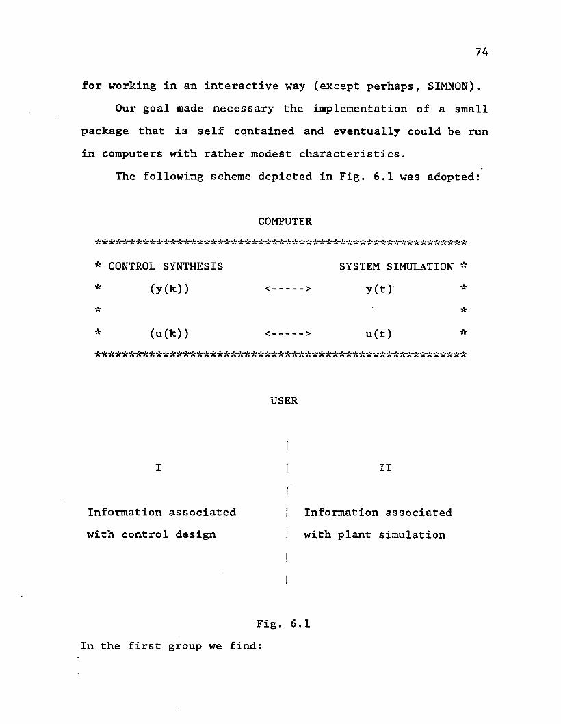
74

for working in an interactive way (except perhaps, SIMNON).Our goal made necessary the implementation of a small

package that is self contained and eventually could be run in computers with rather modest characteristics.

The following scheme depicted in Fig. 6.1 was adopted:

COMPUTER«» «* A «» #« A A O A M A A A A M A A M «« A *» #« M «» <» M «» «» «» A M M A #« <« «« A A A % «« «« A #C«* A «« A A A A

* CONTROL SYNTHESIS SYSTEM SIMULATION ** (y(k)) <... > y(t) ** *

* (u(k)) <.... > u(t) *A A A A A A A A A A A A A A A A A A A A A A A <1 A Ok A A A A «» A A A A A A A A A A A A A A A A A A A A A A A A

USER

I

Information associated with control design

II

Information associated with plant simulation

Fig. 6.1 In the first group we find:

75

Number of inputs and outputs m Order of the model N y and Ng^Sample period hInitial set of estimated parameters 0(0)Stability zone ( A-zone)Gain schedule (for non-linear systems)With the second group we must provide:Number of inputs and outputs mOrder of the plant Nj and Ng (for discrete systems) Differential equations and integration step (for continuous systems)Initial conditionsSet point and load changesSet of inputs for estimation purposes (u(k))Characteristics of noise associated with measurements N(x,a) Open loop identification timeTotal time of simulation (open loop + closed loop)

The only common information between the simulated proc­ess and the control synthesis was the number of inputs and outputs m, the open loop estimation time and present value of vectors y and u.

The simulation package was implemented using structured FORTRAN 77, but only a small number of its features were used such as instructions IF()THEN/ENDIF and DO 100 K = 1, (M**2+M)/2 for instance. These instructions are easy to change if a lower level of FORTRAN is available. Other more

76

powerful characteristics such as arrays with negative in­dexes were not used and therefore the shifted variable y(t-i) is represented by the FORTRAN variable Y(I).

Simulation structureOnce the simulation started, the information about the

system was retained at each sample in a fixed length matrix through a shifting subroutine:

y(t) u(t)I 4

h(t-1)->iII

J Jdiscard discard

Then the regressor vector with variable length, according to the postulated model, was constructed:

= (yT(t-1),...,yT(t-NflM),UT(t-1),...,uT(t-NBH)) where the supra index T means transpose.

The regressor vector and the estimation error vector defined by the product of the matrix of parameters 0 and the regres­sor vector were sent to the estimation algorithm REFIL. The return was the set of polynomial matrices A(z) and B(z). Matrix B was inverted and factored and then the

77

control matrix Gc was computed. Finally, the control vector u(k) was computed according to equation (5.21).

6.2.- OPEN LOOP ESTIMATIONIn this section we present some of the results obtained

with the estimation algorithm without using any control s cheme.

Some parameters must be specified in a heuristic way:a) sampling frequencyb) magnitude of inputc) order of postulated modeld) simulation time

If the system is unknown, several open loop runs are neces­sary. However, this type of process seldom occurs and someinformation is always available. For instance, transient du­ration is a good indicator for fixing the sample interval and the total simulation time. In the same way, the nature of the process gives some clues about the magnitude of the inputs. For estimation purposes, some variable scaling may be appropriate. The estimation algorithm is more accurate working with inputs and outputs of the same order of magni­tude so it is better for instance to work with T/To and C/Cothan directly with T and C.

The order of the model has special importance when dealing with continuous systems with dead time. Our aim was to keep the order as small as possible reducing in this way

78

the number of parameters, but sometimes a large dead time makes necessary a large value to allow the best possi­ble representation. The zero order hold (ZOH) hypothesis was enforced by keeping the vector u(k) constant during the in­tersample time.

Examples6.2.1.- Discrete system. Paper machine headbox The following model is presented by Borison (15)

y (t) + A-,y (t-1) = B-ju(t-l)

with

Ai =-0.9901-0.8061

0.008805•0.770890

Bi =0.8990 -0.00459019.3900 0.880520

6.1We define the above expression as system Bl where

yl = stock levely2 = total pressureul = stock input flowu2 air input flow

We define system B2 with: a(1,1) is reduced in magnitude by 40%

79

b(2,l) is reduced in magnitude by 10%The following parameters were used:Simulated plant:Discrete system B2 for 25<t<61 and 81<t<100

Discrete system B1 any other timeSampling period h: 1 secondInput vector u:PRBS with amplitudes (0.1, 0.2)Initial information matrix P(0) = 10^ IInitial estimation 0(0) = 0Model:The simplest model with =1, Ng^ = 1 was used.The forgetting factor is initially set to one and changes when the estimation error is large. When the parameters con­verge, between time 0 and 25 sec., the forgetting factor re­mains constant near to one. At time 25 sec. two parameters are decreased in magnitude and therefore the estimation error increases modifying the forgetting factor and making the estimation algorithm active. After a while the new pa­rameters have been calculated and the factor returns to one.

IIThe cycle is repeated each time the parameters change.

A very effective adaptation to the new values can be observed in Fig. 6.2.

6.2.2.- Continuous double effect evaporator model A continuous model for a double effect evaporator is pre-

Isented by Newell and Fisher (68): x (1) = -0.00156x(2)-0.1711x(3)-0.143u(2)+0.2174F1 x(2) = -0.14190x(2)+0.1711x(3)-0.74Fl+0.1434CF1

P A P E R M A C H I N E H E A D B O X P A R A M E T E R S E S T I M A T I O N

( O P E N L O O P )

• v a H M O C E L— a l t

-i 0.00

- 1 . 5 00 1 0 2 0 3 0 4 0 5 0 8 0 7 0 SO 9 0 1 0 0T I M E (sec . )

P A P E R M A C H I N E H E A D B O X P A R A M E T E R S E S T I M A T I O N

( O P E N L O O P )

— b 2 1 M O D E L— b 2 1

2 5 - ,

20-

u , 1 5 - a o s- 10-Mn

100

Fi g. 6.2

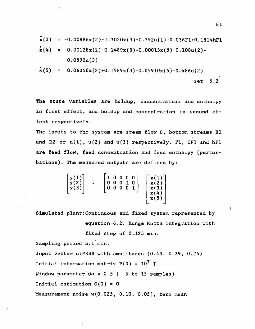
81

x(3) = -0.00886x(2)-1.1020x(3 ) + 0 .392u(l) - 0.036F1+0.1814hFlx(4) = -0.00128x(2)-0.1489x(3)-0.00013x(5)+0.108u(2)-

0.0592u(3)x(5) = 0.06050x(2)+0.1489x(3)-0.0591Gx(5)-0.486u(2)

set 6.2

fyd)] l 0 0 0 0y(2) = 0 0 0 1 0y(3) 0 0 0 0 1

The state variables are holdup, concentration and enthalpy in first effect, and holdup and concentration in second ef­fect respectively.The inputs to the system are steam flow S, bottom streams B1 and B2 or u(l), u(2) and u(3) respectively. FI, CFl and hFl are feed flow, feed concentration and feed enthalpy (pertur­bations). The measured outputs are defined by:

x(l) x(2) x(3) x(4) x(5 )

Simulated plant:Continuous and fixed system represented byequation 6.2. Runge Kutta integration with fixed step of 0.125 min.

Sampling period h:l min.Input vector u:PRBS with amplitudes (0.43, 0.79, 0.25) Initial information matrix P(0) = 107 I Window parameter Cfo = 0.5 ( 6 to 15 samples)Initial estimation 9(0) = 0Measurement noise w(Q.025, 0.10, 0.05), zero mean

82

Model:A(z) = I + A z~1 + A z~ 2 jNjim = 2B(z) = B z”1 + B z-2 ;Ngju = 2

The number of parameters to be estimated is given by NPM = mxm(NAH + NBH ) = 36

Fig. 6.3, 6.4 and 6.5 show the outputs yl, y2 and y3 to­gether with the model outputs yml, ym2 and ym3 respectively. From the figures, we can observe that the model output is hard to distinguish from the plant output after the parame­ters have converged. Finally for this example, Fig. 6.6 shows the evolution of two representative parameters.

6.2.3.-Continuous distillation columnWood and Berry (92) developed a dynamical model of a

pilot distillation column designed to separate a mixture of methanol and water. This model, or slight modifications of it, has been used for control testing purposes, among oth­ers, by Ogunnaike and Ray (71), McDermott and Mellichamp (61) and, Arulalan and Deshpande (9).

The following set of differential equations was used in this work to represent the continuous plant behavior:

x (1) = -0.0600x(l)+(0.7680-0.4012Ind)ul(t-l)x(2) = -0.0476x(2)+(0.9000-0.5000Ind)u2(t-3+Ind)x(3) = -0.0917x(3)+(0.6055-0.2844lnd)ul(t-7+3lnd)x(4) = -0.0694x(4)+(1.3472-0.7361Ind)u2(t-3+2lnd)

Y1

,Y1

MO

DE

L

83

- 0,20--- 0 , 3 0 - ■

- 0 . 4 0 -

D O U B L E E F F E G T E V A P O R A T O R L I N E A R M O D E L Y1MODQ-

0 . 4 0 - 1

0 . 3 0 -

“1---- 1---- 1---- 1-----1---- 1---- 1---- 1---- 1---- 12 0 4 0 6 0 8 0 1 0 0 1 2 0 1 4 0 1 6 0 1 8 0 2 0 0

T I M E ( m i n . )

F i g . 6 . 3

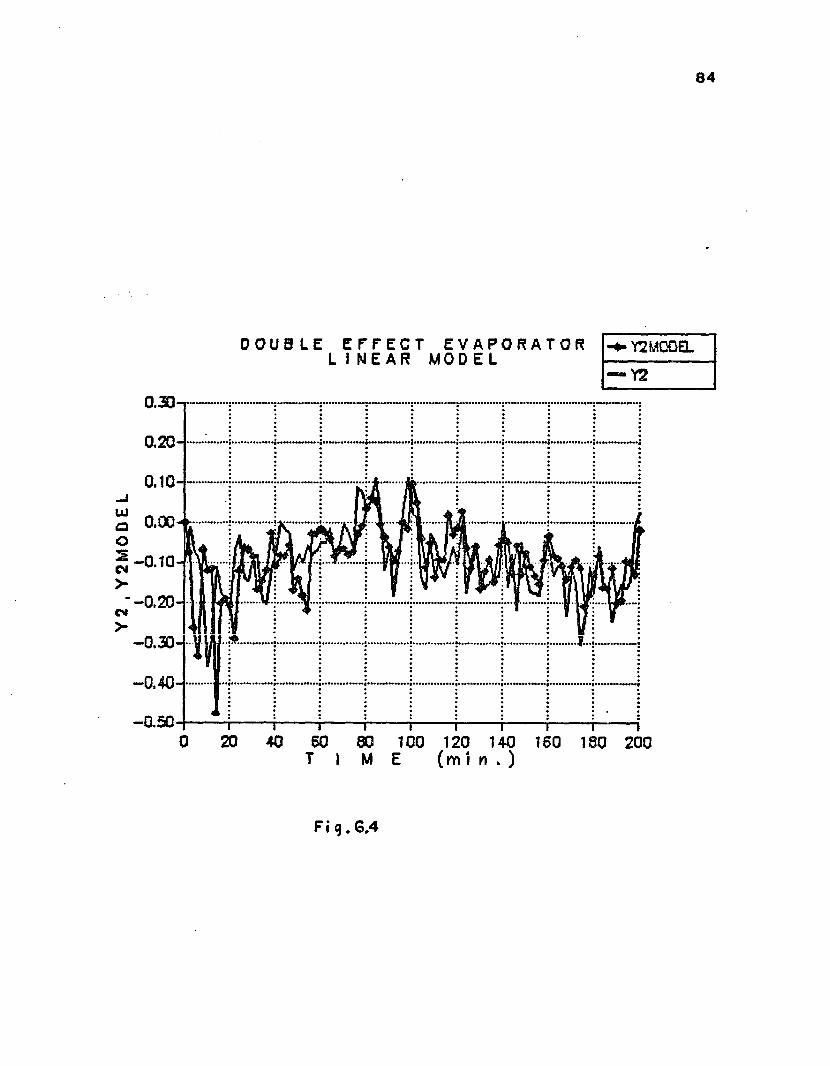
84

D O U B L E E F F E C T E V A P O R A T O R L I N E A R M O D E L Y 2 M O D E L

™ Y 2

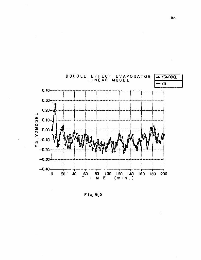
V 3 ,Y

3 MO D

E L

85

D O U B L E E F F E C T E V A P O R A T O R L I N E A R M O D E L Y 3 M O D E L

T 3

0 . 4 0 - 1

0 . 3 0 -

0,20-0.10-

0.00

-0.20-- 0 . 3 0 -

-0.401 0 0 1 2 0 1 4 0 1 6 0 1 8 0 2 0 0

m i n . )T I M E

Fig. 6.5

I

86

D O U B L E E F F E C T E V A P O R A T O R LI N E A R M O D E L a 1 ( 3 , 3 )

— al (1,1?0 . 8 0

0 . 4 0 -

0.20-oZ 0.00

o

— 0 . 6 00 2 0 4 0 6 0 8 0 1 0 0 1 2 0 1 4 0 1 6 0 1 8 0 2 0 0M E

Fig. G.6

87

x(5) = -0.0671x(5)+ 0.2550F(t-8)x(6) = -0.0768x(6)+ 0.3712F(t-3)

set 6.3y(l) = x(l)-x(2)+x(5) y (2) = x(3)-x(4)+x(6) bottom composition

top composition

ul reflux flow rateu2 steam flow rateF feed flow rateInd = 0 if F = 0Ind = 1 if F = 0

The purpose of Ind is to simulate a plant change when the feed flow rate is changed. It is assumed that the properties of the column most affected by feed flow changes are static gains and dead times. This is a reasonable assumption pro­vided the dynamic lags (time constants) are less sensitive to flow changes in the plates and that no flooding occurs.J In terms of matrix transfer functions the system is re­presented by:

SI:12.8 exp(-s) -18.9 exp(-3s)

16s + 1 21s + 1y(s) = u(s) 6.46.6 exp(-7s) -19.4 exp(-3s)10.9s + 1 14.4s + 1

88

S2:

y(s) =

6.1 exp(-s) - 8.4 exp(-2s)16s + 1

3.5 exp(-4s) 10.9s + 1

21s + 1 8.8 exp(-s ) 14.4s + 1

u(s)

3.8 exp14.9s

4.9 expF(s) 6.5

13.2s + 1

The time constants are in minutes.Simulated plant : Set of equations 6.3. Runge Kutta

integration with fixed step of 0.125 min. Sampling period h: 1 min.Input vector : white noise with zero mean and variances

(0.025, 0.02)Initial information matrix P(0) = 10^ I Window parameter CFo =0.005 Initial estimation 9(0) = 0 Model orderFig. 6.7 presents the average estimation error for different values of parameters and Ng^ . The average error wasdefined as:

( e ) Z (e2(l) 1 K

+ e*

M E A N E S T I M . E R R O R

N -

Ul -

G>

ZCD

U» -

c n -

"■J -

CO - J

HOC

'I.

OO

'Z

1 0NJrmo

OGO H

SC — O l ~Ol-m >f - Ho oom o;uor~cs;

4Z

4z

4z

> > >li II II—j . r o Ul

90

The smooth curves should be understood as plotter character­istics. Only the integer values make sense.The models will be denoted Cij, C for column and i, j for the parameters and respectively.The local minimum estimation errors are obtained for i =1,2,3 and j = 3;i = 1,2 and j = 4,6;i = 1,2, 3 and j = 7.That is, there are at least 10 models with similar esti­mation error. Obviously, model C14 must be preferred to model C37 for example, that gives similar average error but needs 40 parameters instead of 20.Open loop response

Figs.6.8 and 6.9 show the open loop response of the process together with the model output. The model is esti­mated on-line.

The vector y(k) represents the output at sampling timek.

The vector ym (k) represents the output of the discrete model G# at sampling time k. That is :

ym = A”1 Bu = G#uwhere A and B are the estimated polynomial matrices, and u is the same input vector that drives the plant.Models C13, C14, C16 and C27 were tested and no perceptible difference can be observed for the top composition y(l). For bottom composition y(2), models C13, C14 and C16 show small differences between y(2) and ym2.

*1

.j 1

MOD

EL

*1

.jM

MO

DE

L

D I S T I L L A T I O N C O L U M NO P E N L O O P R E S P O N S E

MODEL C13 — yiuoca■yt

0 30 40 SO 89 100 130 140 ISOT I M E ( m i n . ) 180 300

MODEL 013 •vySMOEL

- y »

a aaaaA aa«iaaaa^aaaaM »H 4aaB aaaaaaA aaaaaaaa|aaaaaa# |a |aa4 |||si||ia |aai« |^

&15C-

-0 .1 3 9 -

~i— »— t— ,“r— i— «— i— r— T" “i 0 30 40 60 SO 100 130 140 ISO 1g> 390T I M E ( m i n . )MODEL C14 ■ylUOOEL

0 3) 40 SO 80 IOO ISO 140 ISO 180 390T I ME (min.)

MODEL 014

F I 9 . 6 . 8

0.140-

1---1-1 1 1---- 1 180 100 130 140 ISO 180 300 M E (min. )

<0

y 1

,y 1

MO

DEL

y^

,y

1 M

OD

EL

D I S T I L L A T I O N C O L U M NO P E N L O O P R E S P O N S E

MODEL Cie

aioo-

0 30 40 DO 00 100 I S 140 160 180 300

— yIMDDa MODEL Cle *»y2HOOEl— yl — y3

T I M E (rain.) (rain.)MODEL C27 "vylMOOEL MODEL 027 vySMODEL

-yl — yt

0 39 40 60 ft 1DO 130 140 160 180 300T I M E (rain.) Fi q.6.9t — i— ”1-------1------1— i-------1------1— I40 60 <9 100 I3D 140 160 Itt 390 T I M E (rain.)

93

6.3.- CONTROL APPLICATIONSA standard procedure was established for testing the

control algorithm. We assumed the minimum knowledge aboutthe process and started all the simulations in an open loop form with the same parameters used in the previous section.

After a number of identification samples that is chosen according to the model size, the system was switched to con­trol mode and the input vector u was generated through the IMC structure. The changes in the set point and perturba­tions were started once the system was working in automatic.

Two set of additional parameters were necessary:1) Filter parameters di

These parameters were set initially at 0.5 and then were changed by trial and error. Normal operating ranges were found between 0.3 and 0.8.2) Estimation error threshold

An average open loop estimation error was calculated.After switching to automatic, this value was used as anindex in such a way to by-pass the calculation of the con­trol structure if the model has not been updated. This pro­cedure improves the computation load.

6.3.1.- Paper machine headboxThe system B1 described in 6.1, although very simple,

has some undesirable characteristics that make it difficult to control by conventional methods.

94

In Figs. 6.10a and 6.10b we can observe the open loop response when the process is forced to a new operation point by the application of a constant input vector u calculated as G(l) y* where y* is the new operating point. One of the output variable shows a very slow transient while the second output presents inverse response added to the slow tran­sient .

In Figs.6.11 and 6.12 the performance of the adaptive multivariable internal model control is shown. During the first 20 samples the inputs to the system consisted of PRBS with amplitudes 0.01 and 0.02. The outputs were corrupted with white noise sequences with variance 0.010 and 0.020. Then the inputs were switched to those generated by the IMC algorithm and a sequence of set point changes was started:

sp(1) = 2.15(r(19)-r(57)+r(82)) sp(2) = 1.80(r(25)-r(62)+r(82))

where r is the unit step function. The total decoupling and almost perfect set point tracking can be observed. Although the same behavior can be obtained with a fixed non adaptive controller designed following the internal model structure for a known plant, we must point out the complete self-tu­ning characteristic of our system.

Figs. 6.13 and 6.14 show the performance of the fixed non adaptive IMC system when the plant is changed from the

95

P A P E R M A C H I N E H E A D B O X O P E N L O O P R E S P O N S E

Q 20 40 60 60 tOO 120 140 160 !60 200T I M E ( s e c . )

0 20 40 60 60 too 120 140 160 160 200T I M E (sec.)

F«q. 6.I0

96

a.w

4T

3--

2-

1--

-14

- 2-

P A P E R M A C H I N E H E A D S O X M U L T I V A R I A B L E A D A P T I V E I M C — S p 1

— yi~

T “10 20 30T I

I T"40 50M E 60 70 80

( s e c . ) .

90 100

F I g . G . l l

97

P A P E R M A C H I N E H E A D S O X M U L T I V A R I A B L E A D A P T I V E I M C — *sp2— y2

CMa.

CM

-14

-21 0 2 0 3 0 4 0 5 0 6 0 7 0 8 0 9 0 1 0 00

Fi g. 6.12

98

P A P E R M A C H I N E H E A D B O X NON A D A P T IVE IMC

( C H A N G I N G P A R A M E T E R S ) — y1

a.

-2

Fi <J • 6*13

99

P A P E R M A C H I N E H E A D B O X NON A D A P T I V E IMC

( C H A N G I NG P A R A M E T E R S )sp2

— y 2

CM 2 -

CM

0 1 0 2 0 3 0 4 0 5 0 6 0 7 0 8 0 9 0 1 0 0

Flq. 6.14

1 0 0

original system B1 to the new system B2. This change simu­lated a variation of plant parameters each time the total pressure (sp2) was moved to values different from zero. The change was achieved by decreasing the magnitude of a(l, 1) and b(2, 1). Although the change is moderate, the fixed IMC is completely deceived and the response is unsatisfactory.

We can point out that this is one weakness of the non adaptive internal model structure. According to the theory, condition (3.25) is accomplished and the global system is bounded input bounded output (BIBO) stable, but due to the parameters change, the process is non-linear and BIBO sta­bility doesn't mean asymptotic stability any more. There­fore, the tracking properties are lost, and furthermore, this simple example shows that BIBO stability is a weak con­dition.

On the other hand, the adaptive multivariable IMC shows in Fig. 6.15 that after some samples, the new system was identified with a performance equivalent to that obtained with open loop test (Fig. 6.2). Therefore the control is re­covered with satisfactory set point tracking as shown by Figs. 6.16a and 6.16b. Finally, Fig 6.17 shows the control requirement for the latter example. One of the manipulated variables, air flow u2, is for one sample far outside its normal range. We must recall that the system has been dras­tically forced to follow the set point, overcoming the slow dynamic and the inverse response characteristics. A better

101

P A P E R M A C H I N E H E A D B O X P A R A M E T E R S E S T I M A T I O N

( C L O S E D L O O P )

- v a i l MODEL

— a l lO.SO-i

0.00

-0 .50-

1.500 10 20 3) 40 50 80 70 00 90 100T I M E ( s e c . )

25-1

20-

_ihj 15 O O 3- 10H<NSI<N

P A P E R ' M A C H I N E H E A D B O X P A R A M E T E R S E S T I M A T I O N

( C L O S E D L O O P )

« ^ b2 1 MODEL

— b 2 1

v k .

J10 20 30

T I40 50M E

60 70( = = c • )BO 90 100

Fi g. G.l 5

102

P A P E R M A C H I N E H E A D B O X A D A P T I V E M U L T I V A R I A B L E I M C

a.

10 20 30 40 50 60 70 BO 80 1000T I M E ( s e c . )

P A P E R M A C H I N E H E A D B O X M U L T I V A R I A B L E A D A P T I V E I M C

a.

- 1-

0 10 20 30 40 SO 60 70 BO 80 100T I M E ( s e c . )

F i g . 6.16

103

P A P E R M A C H I N E H E A D B O X M U L T I V A R I A B L E A D A P T I V E I M C uZul

10-

- - 10-

- 20-

-30-

40 50 60 70 80 90 100T I M E ( s e c . )

Ficj. 6.1 7

104

behavior for the manipulated variable can be obtained by in­creasing the filter parameters making the controlled system more sluggish.

6.3.2.- Distillation columnIn the first place we tested the self-tuning IMC by in­

troducing the following set point vector:

sp(1) = 0.8*r(30)sp(2) = 1.6*(r(30)-r(155))

Then, the adaptive properties were tested by changing the plant characteristics from system SI to system S2 after in­troducing a load disturbance at time = 80 min.and the fol­lowing set point:

sp(1) = 0 .8*(r(30)-r(57)+r(160)) sp(2) = 0.F = 0.34*r(80)

The control action was started after 30 samples and all the variables must be understood as deviations around a steady state.

Set point changeFigs. 6.18 to 6.21 show the closed loop behavior for

different models under adaptive internal model control. All

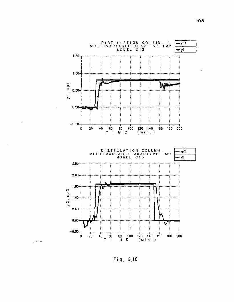
105

D I S T I L L A T I O N C O L U M N ' — aptM U L T I V A R I A B L E A D A P T I V E I M C Z _

M O D E L C 1 3 — yl

1 .SO-.

i .00-

a.“ 0 .5 0 -

0.00

- 0 .5 00 20 +0 60 BO 100 120 140 160 1B0 200T I M E (min.)

D I S T i L L A T I O N C O L U M N MULTIVARIABLE ADAPTIVE IMC M O D E L C 1 3

1.50(Na.<a

1.00

0.50

0.00

0.5020 4i] 60 BO 100 120 140 160 1B0 2000

F i g . 6 . 1 8

106

D I S T I L L A T I O N C O L U M N — *p1M U L T I V A R I A B L E A D A P T I V E I M'C --_M O D E L C 1 4 — <yi

! .50-1

1.00-*

-0 .5 020 40 60 BO tOO 120 140 160 1B0 2000

T I M ~ E ( m i n . )

DISTILLATION COLUMN M U L T I V A R I A B L E A D P T i V E I M C

M O D E L C 1 4

'«p2

00'

1.50-■N£3." 1 .00 -

^ 0 .5 0 -

0.00'

100T I M E ( m i n .1

F i g . G. I 9

107

D I S T I L L A T I O N C O L U M N — SP1M U L T I V A R I A B L E A D A P T I V E I M C -----------

M O D E L 0 2 3 . •••Y1

1.50

1.00- •

a.11 0.50

0.500 20 +0 60 SO 100 120 1+0 160 1BQ 200

T I M E i n . )

D I S T I L L A T I O N C O L U M N M U L T I V A R l A B L E A D A P T I V E I MC

M O D E L C 2 3

■ s p 2

2.50-1

2 .00-1

1 .50-

1.00-

0 .5 0 -

-0.50.0 20 +0 60 BO 100 120 1+0 180 IB ! 200

M E [ m i n

Fig. 6.20

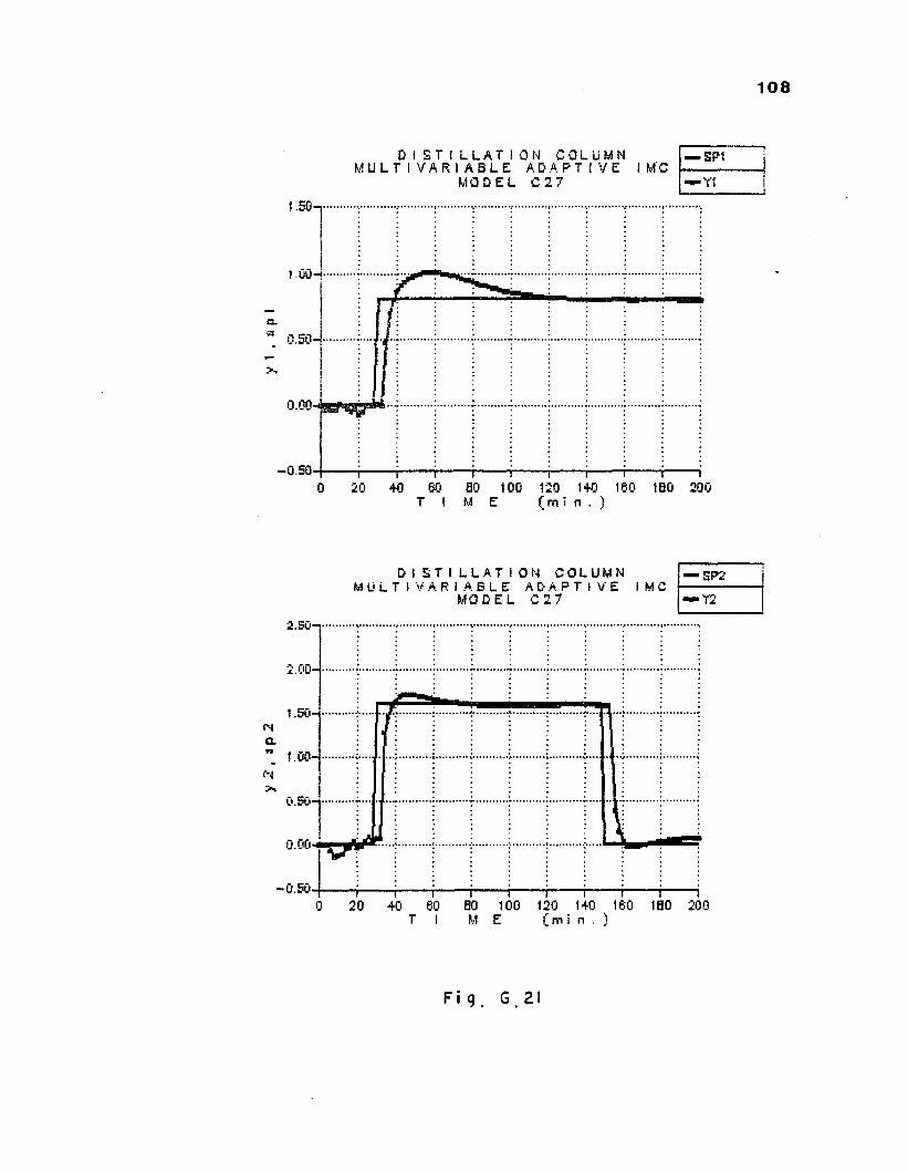
108

D I S T I L L A T I O N C O L U M N M U L T I V A R I A B L E A D A P T I V E I IrfC

M O D E L 0 2 7

■ EP1

■ Y1

1.00-

0.50-

0.00'

-0 .5 00 2 0 40 60 BO 100 120 140 160 1B0 200T I M E f m i n . )

D I S T I L L A T I O N C O L U M N M U L T I V A R I A B L E A D A P T I V E I M C

M O D E L C 2 7

— SP2

■Y2

00-

1 .50-

1.00-

0.00

-0 .5 020 40 60 B0 100 120 140 160 1B0 2000

T I M E I. m i n . )

F i g . G . 2 I

109

the tested models lead to highly decoupled control. This de­coupling and the smoothness of the response increase as the parameter Ng^ increases.

The filter parameters were set to 0.60/0.70 for model C13 and C23 and 0.65/0.75 for models C14 and C27 (trial and error).the estimation parameters were set at the same values used for the open loop test.

Load and system changeA step change in the feed stream was introduced. This

sustained perturbation means also a change in the system dy­namics that will be represented by S2 (6.5) instead of Si (6.4).The estimation problems that a deterministic load poses, can be explained through the following scheme:

EST. AL6.

P R O C E S S

M O D E L

Fig. 6.22 Load Effects

1 1 0

The algorithm cannot establish the difference between a load disturbance or an eventual process parameters change (though in this test the change is more severe because the load also implies process gains and time delays modifications).The load can be accounted for by the introduction of ficti­tious parameters to be estimated:

if y = Gu + d - y + dwhere d represents the load, then:

A 4 ^y = A-1 Bu + d is the estimated output vector whileA Ad is the estimated load (do not confound y with ym the model output).y can be expressed as:

y = 0 0 with

0 - (A-j, • * • , ’ • • • > i 6 ) and

$ T = (yT(t-l), . ,uT (t-1), . . .uT (t-NBH ), 1)ExampleA simple single input single output example will help to un­derstand the preceding statement:

z - 0.5z“2Let G (z-1 ) = --------------------

1 - l.4z“1 + 0 .4 8 z~2

Ill

and y(k) = 1.4y(k-l)-0.48y(k-2)+u(k-l)-0.5u(k-2)+e+d

where e is a white noise sequence and d is a deterministic load.Fig. 6.23a shows the estimated parameters when the standard recursive least square algorithm (RLS) is used and no load affects the process.

At this stage, y = Gu and ym = G#u differ only in the white noise since the estimated parameters are very close to the true parameters.Fig 6.23b shows the same system with a load equal to 17.5% of the input amplitude. After the load is introduced, the estimated parameters are biased, yffl is no longer equal to y and a large modeling error is produced.Fig. 6.23c shows the performance of the modified RLS with a fictitious parameter added to the estimation and a component of value one added to the regressor vector. This extra pa­rameter lumps all the effects of the load in such a way that the other parameters are unchanged.So ym = y and y - y^ = d , estimated load. This estimated load is important because it corresponds to the feedback signal to the IMC controller. Of course, we cannot differentiate between load and modeling error, therefore if the model is a bad representation of the system, the feedback signal is contaminated. Our conjecture is that adapting the model to follow the plant changes, makes IMC more robust.

112

P A R A M E T E R S E S T I M A T I O N S T A N D A R D R L S W I T H O U T LOAD

2

!■"18-l- 2-1

b 1 a 2

b 2 a 1

— I---- I ! I T I I I I I9 19 2 9 J 9 4 0 9 9 W I 7 9 4 9 9 Q 1 9 9

P A R A M E T E R S E S T I MAT I ON S T ANDAR O R L S Wl TH L 3 AD

2t

- 1-

-2-

0 10 20 40 10 W «0 70 m W I00

j w m ' V i / V i w m

- 1-

-2-

0 10 20 40 40 «0 TO «0 40 10Q

Fi q. G . 2 3

113

The changing parameters are detected with the use of a variable forgetting factor and making the algorithm more sensitive by decreasing the observation window (decreasing uo) .

Fig. 6.24 shows the actual load d = F for a step change of 0.34 lbs/min in the feed stream. It also shows the dif­ference y-ym (d following the IMC nomenclature). It is evi­dent that the load identification is satisfactory.In the next test , a different sequence of changes in set point was used, with sp2 = 0. This is a known difficult test (see McDermott and Mellichamp (62)) because of the lack of persistent information for one of the inputs. At time 80 minutes, the step load was introduced and the process was changed to S2. Fig. 6.25 shows how the proposed control was able to overcome the load effects and the system modifica­tions. By the way, the slow rejection of the load is a prob­lem proper of the IMC structure whenever the system dynamics is slow (the transient corresponds to the open loop re­sponse). This problem was pointed out by Svoronos (83) while working with single input single output systems.

Effect of persistent signalsFigs. 6.26,6.27,6.28, and 6.29 show the performance of

the proposed adaptive internal model control when the proc­ess is forced to a new operating point by changing both set points and at the same time a sustained load is applied at

41

,41

0o

t 41

■ 41

0

01114

D I S T I L L A T I O N C O L U U M LOAD ESTI N A T I O N

m «4 4 l 0 1 4 KOI

■CJt-40 40 40 100 12© 140 140 140 300 T I M E {fllln . )

D I S T I L L A T I O N C O L U U M LOAD E S T I M A T I O N

R I0 4 4 I 0 1 4 — 42

40 100 120 140 140 140 200 M E {mill ■ )

0 20 40 40

D I S T I L L A T I O N C O L U M N LO AD E S T I M A T I O N

m « 4 « I 0 1 4— 4144T— 41

144 140 200

D I S T I L L A T I O N C O L U M N LOAO E S T I M A T I O N

RI44 4 I 0 1 4

- 140-

OOO-140 140 290

F i q . 6 . 2 4

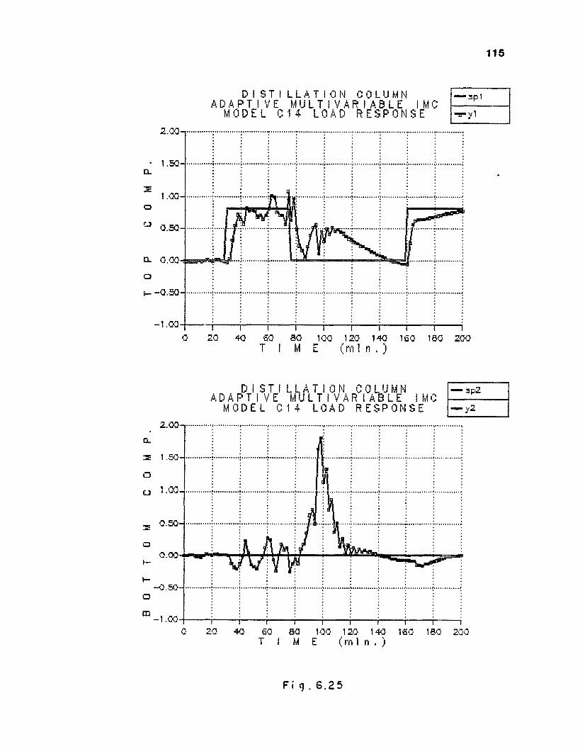
115

D I S T I L L A T I O N C 0 L U MNA D A P T I V E M U L T I V A R I A B L E I M C

M O D E L C 1 4 L O A D R E S P 0 N S E■=pi

• vl

o° 0.50-

-1.0020 40 60 SO 100 120 140 160 180 200

T I M E C m l n .

D I S T I L L A T I O N C O L U M N A D A P T I V E M U L T I V A R I A B L E I M C MODEL 014 LOAD R E S PONSE

— s p 2

2 .00-1Cl

0.50-

O

-0.50-

- 1.000 20 40 60 80 100 120 140 160 180 200

T M E ( m l n , )

Fig. 6.25

116

D I S T I L L A T I O N C O L U M NA D A P T I V E M U L T I V A R I A B L E I M C

M O D E L C 1 3 L O A D R E S P O N S E— =pi

■ vl

-1 .coo 20 40 SO SO 100 120 140 ISO ISO 200

M E ( m I n . )

D I S T I L L A T I O N C O L UM N ADAPTIVE M U L T I V A R I A B L E IMC M O D E L C 1 3 L O A D R E S P O N S E

1 sp2

3 2.00-

O1.50-

0.50-

-0.5020 SO SO 100 120 140 ISO ISO 200

T M E ( m I n . )

Fi cj. 6 . 2 G

117

D I S T I L L A T I O N C O L U M NA D A P T I V E M U L T I V A R I A B L E I MC

M O D E L C 1 4 L O A D R E S P O N S E

— spi

■yl

2 .00-1

z1.0 0 -

° 0 .5 Q -

D- 0.00

l— - 0 . 5 0 -

- 1 . 0 0

o € 0 SO 100 120 140 1 6 0 180 2 0 02 0 4 0T I M E ( m ! n . )

D I S T I L L A T I O N C 0 L UM N A D A PTIVE M U L T I V A R I A B L E IMC M O D E L C 1 4 L O A D R E S P O N S E

■Sp2

— y22 .5 0 - ,

3 2.00-

1.50-

0 .5 0 -

0.00

- 0 .5 00 20 6 0 SO 1004 0 20 140 160 180 2 0 0

T I M E (mIn.)

F i g . 6 . 2 7

118

D I S T I L L A T I O N C O L U M NA D A P T I V E M U L T I V A R I A B L E I M C

M O D E L C 1 6 L O A D R E S P O N S E— s p l

' v l

2.00-,

o0.50-

-1.0020 40O 60 50 100 120 140 160 180 200

T M E ( m l n , )

D I S T I L L A T I O N C 0 L U MN A D A P T I V E MU L T ! V AR I AB L E I M C MODEL C 16 LOAD RESPONSE

>sp2

y2

CL

3 2.00'

O

Ol—t—OCD

-0.5020 40 60 50 100 120 140 160 180 200

M E ( m l n . )

F i g . G . 2 9

119

D I S T I L L A T I O N C O L U M NA D A P T I V E M U L T I V A R I A B L E I M C

M O D E L 0 2 7 L O A D R E S P O N S E

o

CL 0.00

.50

1.00Q 60 60 100 120 140 ISO 150 200

T I M E ( m 1 n . )

D I S T I L L A T I O N C O L U M N ADAPTIVE M U L T I V A R I A B L E IM C M O D E L 0 2 7 L O A D R E S P O N S E

aP2

— Y2

CL

3 2.00-o

1.00-

0.50-

0.00

60 100 120 140M E ( m 1 n

Fi q . 6 . 2 9

1 2 0

time = 80 min. This load means, as it did before, that the plant characteristics change from system SI to system S2. In this example, the robustness of the proposed control scheme can be observed with its capability to handle strong pertur­bations. It must be pointed out that whenever the informa­tion is persistent exciting, that is there exists sufficient information for determining the parameters, the adaptive in­ternal model controller offers a great flexibility with re­spect to the model order. Four reasonable models show good performance under the same perturbation conditions.

6.3.3.- Non-linear chemical reactorWe can say that all physical systems are non-linear and

time variant, but the most common way to represent them, is through linear and time invariant models. This is possible, and the models will describe adequately the process, as long as the non-linearities are mild and the deviations from the operating point are small.

Sometimes, nevertheless, the linear model is not able to predict in a correct form the behavior of a process. In this case, other representations, like bilinear forms or the use of non-linear estimation methods are necessary. Though more mathematics is involved, the non-linear models consti­tute a rich source of possibilities and the results justify their use. In order to set a boundary in the search of mod­els and, for creating reasonable structures, a deeper in­

1 2 1

sight into the physical character of the non-linearities is necessary.

When dealing with symbolic mathematics i.e. block dia­grams for linear or non-linear systems, our aim is to get the maximum knowledge about interconnected subsystems, starting from the knowledge of how each separated subsystem behaves. There are three elementary connections known as tandem, parallel and feedback. All other ways can be ob­tained as combinations of these elementary forms.

The most important properties of a system, i.e. stabil­ity and characterization are preserved through parallel con­nection. In case of tandem connection some problems arise with characterization of the whole system;some information may be lost due to pole-zero cancellation (for linear sys­tems). The most complicated case, corresponds to the feed­back connection where open loop characterization and stability, does not ensure these properties will be main­tained when the loop is closed.(Indeed, a great part of the control efforts consist of how to design a subsystem so that it will produce a stable system when connected in a feedback path).

Stability may be established for linear invariant sys­tems using Nyquist criterion, provided the process is SISO and known.Some extensions of this criterion have been devel­oped for multivariable conventional systems (Arkun et al.(8)). The stability finally depends on the gains or am­

1 2 2

plification of the signals and phase delays while the infor­mation is flowing around the loop. Zames (96) successfully links the Nyquist criterion to the behavior of feedback es­tablishing "that the stability of non-linear, time varying systems can often be assessed from certain gross features of input-output behavior, related with amplification and delay". Therefore, a general feedback system is closed loop stable provided the open loop gain is less than unity. As simple as is this criterion, though conservative sometimes, it constitutes a powerful design tool.

The above stability properties are general for any kind of feedback control. Besides, we must recall that the IMC structure is completely equivalent to conventional feedback control after redefining the control transfer function. Applications to internal model control structure.

The first step towards the design of a non-linear con­troller with internal model compensation corresponds to Eco- nomou et al.(26) who work with a single input single output known system.

The class of non-linear systems we are dealing with, is represented by the following operator equation:

x = f(x) + g(x)uy = h(x) 6.6

where f, g and h belong to some fields on R . Economou et al (26) develop an inverse operator of (6.6) using a numerical

123

procedure based on the work of Hirschorn (40).The developing of a right inverse operator is also stu­

died by Nijmeijer (69) following a geometrical approach. Though the conditions for inverting the operator are impor­tant, in both cases, the algebraic and the geometrical ap­proaches, the amount of mathematical manipulations is so cumbersome, that any other approach seems to be more desira­ble. Besides, a heavy knowledge of the structure and parame­ters of the system is absolutely necessary.(We must recall that the lack of adequate models is one of our problems). An alternative way of synthesizing non-linear controllers was explored by Kravaris and Chung (51). They apply the Lie de­rivative and brackets to get a linear system after using a non-linear transformation, the controller is designed over the linear system and then they come back to the original non-linear process. Once again, the necessary knowledge of the process and the mathematical complications make this method impractical.IMC analysis.-

Returning to the internal model control structure, we can state that it is more important matching the model out­put to the plant output (opening the loop) than getting the exact inverse of the plant operator.

Assume P represents the non-linear plant and that G# is a linear model approximation such that | | Pu - G#u| | < cwhere u is the control vector and the norm is Euclidean.

124

Note that, up to this point, no requirements have been im­posed on c, except being greater than zero. Later, a small c will mean a good modeling of the plant.For a plant P the IMC structure gives:

u = (I-GcG#)"1 Gc(sp-y).So, if Gc = G#"1 , the output y is independent of the givenplant. That is, an infinite gain is achieved and the system will suffer from stability and sensitivity problems, unless c = 0, and that means the perfect modeling we know we cannot obtain.

The independence of y from G is true after the follow­ing:For IMC systems

y = G(I + Gc(G-G#))“1Gc(sp-d) + d

assume the model is not accurate and G# is a bad represen­tation of G.Construct Gc = G# then:

y = G(I + GcG - I )“1Gc(sp-d) + d = sp

This is possible because the gain is infinite or I-GcG# = 0. Since the model is not accurate, y -y £ 0 and therefore the controlled process will be very sensitive or unstable.

125

A more simple approach under adaptive IMC structure

The basic aspect of IMC structure is to calculate a model output ym such that it matches the plant y (in absence of load disturbances). An adaptive linear model can produce the appropriate matching output ym nevertheless, the inverse operator for the linear model cannot match the inverse oper­ator of the non-linear plant.By this reason, the synthesis of the "perfect" controller must be abandoned and a differ­ent way must be sought.

Let us study the following non-linear reactor presented by Tsiligiannis and Svoronos (86).

Ca - F(Cao-Ca)/V-ko*exp(-E/RT)Ca

T = F(To -T)/V+(-DH/pcp)ko*exp(-E/RT)Ca-UA(T-Tc)/Vpcp withA : heat transfer areaCa : reactant concentrationCao : feed concentrationcp : specific heat

-DH : heat of reactionE : activation energyF : flow rateko : frequency factorR : gas constant

126

T : reactor temperature Tc : coolant temperature To : reference temperature U : overall heat transfer coefficient p : density

Defining x(l) = Ca/Cao x(2) = T /To u(l) = F /Fo u(2) = Tc/To

we have

x(l)x(2)kab

= (l-x(l))*u(l)/Tau - kx(l)= (l-x(2))*u(l)/Tau + akx(l) - bx(2) + bu(2) 6.7 = ko*exp(-g/x(2)) 6.8= -DHCao/Vpcp= UA/Vpcp

g = E/RToTau = V/Fo

The measured outputs are:y(l) = x(l)(t-2) dimensionless concentrationy(2) = x(2)(t) dimensionless temperatureAssuming the system is completely unknown, a first at­

tempt was to represent the non-linear plant P by a linear model G# with = 1, = 4 and then construct Gc as thebest inverse of G#. Though the values of c are very small

127

(but £ 0), constructing Gc = G#"1 G+ means a high gain and therefore the controlled system is quite sensitive and prone to instability.Figs. 6.30 and 6.31 show the best results for a step change of 0.5 units in the dimensionless concentration while the temperature set point remained constant. Although the filter F has been tuned with a strong damping effect, the results aren't satisfactory.

The offset is due to the fact that G#~1 (1) is not the true inverse of P(l). Even though c is very small and d ~ d, the inverse of the linear model doesn’t match the inverse plant operator. The high sensitivity is caused by the high gain controller.

Improving the non-linear IMCThe reactor model (6.7) belongs to a more restricted

class of systems than those defined by (6.6). As a matter of fact, we can rewrite (6.7) as :

• '-k 0 ’ (1-xl)/Tau 0X = x +

ak -b (l-x2)/Tau bor

x = A(x)x + B(x)uy = h(x)

x, y c R2Equation (6.9) is not a bilinear system, in spite of

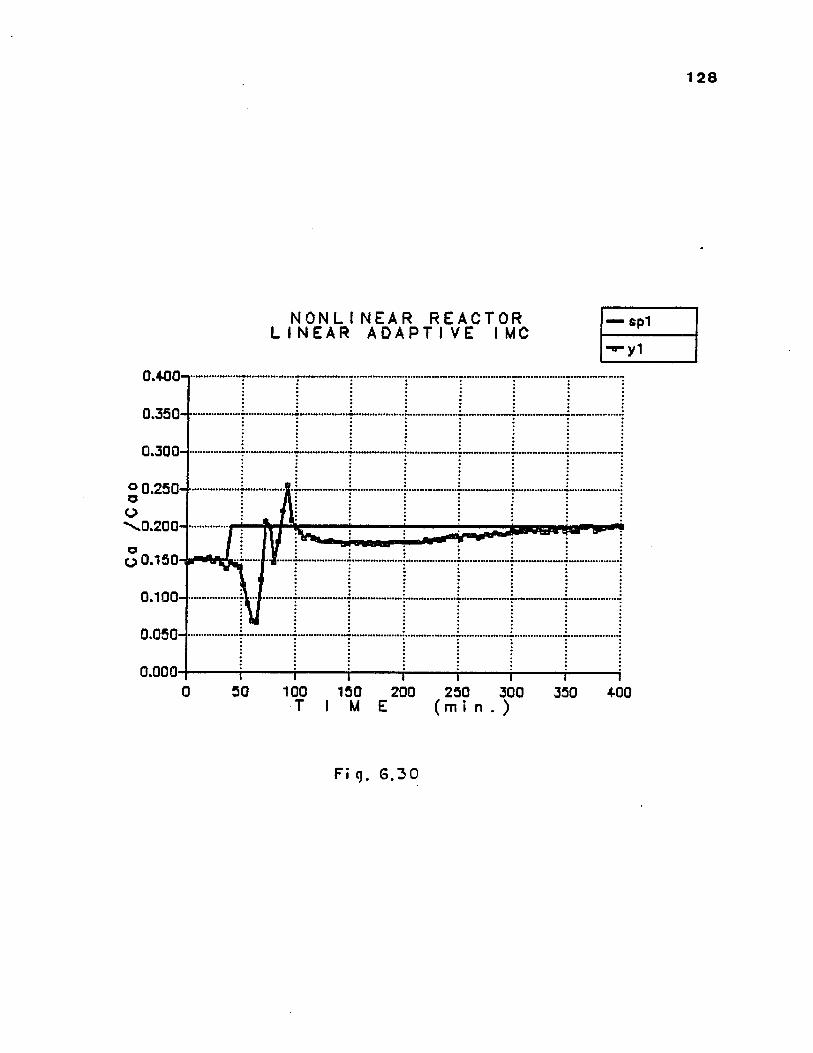
0 D

1 28

N O N L I N E A R R E A C T O R L I N E A R A D A P T I V E I M C sp1yi

0.300

0.250

150

100

0.050'

0.0000 SO 100 150 200 250 300 350 4-00

Fi q. G.30

129

N O N L I N E A R R E A C T O R LI N E A R A D A P T I V E I M C

1.150-

i—

1.050-

1.0000 50 100 150 200 250 300 350 4-00T I W E (m i n . )

Fig. 6.31

130

its aspect, due to the presence of the highly non-linear term k = ko*exp(-g/x(2))At steady state, we can write:

xs = -A"1 (l)*B(l)us = G k u s 6.10

Gjj is not a transfer function matrix nor a differential op­erator but just a numerical gain matrix relating xs and us . The argument 1 in matrices A and B means that their evalu­ation must be done at time = oo assuming for x(l) and x(2) the required set point values. In practice, this asymptotic behavior is obtained by evaluating at each sampling time with the present set point values.Having obtained the steady state gain matrix, Gc is designed as :

Gc = G""* F where F is the IMC filter.In this way, we can estimate on line an adaptive model G#that makes it possible to follow the plant evolution for different operating points in such a way that =" y andtherefore the system behaves as open loop according to theIMC structure. This allows us to design Gc with the only re­striction that it must be stable.In Figs. 6.32 and 6.33 using the same model as before, we can appreciate the improved behavior of the system with re­spect to Figs 6.30 and 6.31.

131

RemarkThe uncertainty about the parameters a, b, g and ko,

can be eliminated by estimating them through the use of the same RLS algorithm with non-linear regressors (though the model itself is non-linear, ko is linear with respect to the regressor exp(-g/x(2)) and g is linear with respect to l/x(2)). For more details about the non-linear estimation see Agarwal and Seborg (1, 2). It is not necessary to carry on this procedure on line because for a given system, the parameters are constant or almost constant. For example, g = E/RTo and E is known to experience small variations with temperature, but normally, the changes mean effects that are far beyond our accuracy measuring the temperature in an in­dustrial process.

132

N O N L I N E A R R E A C T O R A D A P T I V E G A I N S C H E D U L E I M C sp1-»-yi

0.400-

0.350

0.300

« 0.250-

0.100

0.050-

0.0000 50 100 150 200 250 300 350 400

Fi g . 6 .3 2

133

N O N L I N E A R R E A C T O R A D A P T I V E G A I N S C H E D U L E I M C1.200-

1 .1 5 0 -

1.100-

1 .0 5 0 -

1.000- iSO

— s p 2y 2

f—I--

--1

i ...!.

...i

in.—

1 00 1 5 0 2 0 0 2 5 0 3 0 0T I M E ( m i n . ) 350 4-00

Fig, S.3 3

CHAPTER VII

DISCUSSION AND CONCLUSIONS

The performance of the proposed adaptive multivariable in­ternal model control must be discussed from several points of view.

1.- ModelingOne of the points extensively discussed by Foss (30) is

the difficulty of representing large multivariable processes by low order models. We can say that the phenomenological approach, that is the estimation of parameters without phy­sicochemical meaning, fulfills the modeling needs and is completely adequate for control purposes. Furthermore, fix­ing a priori a matrix structure means transforming the iden­tification problem into an estimation one with the order of the model as a unique parameter to specify. This scheme adds the necessary flexibility when dealing with large systems. In all the worked examples, the matching of the plant output y and the model output yffl was outstanding. We refer to matching the outputs instead of parameters because the "true" parameters do not exist for continuous systems and the estimated parameters for a discrete model are valid only for a given order with no other meaning as explained above. Another important reason is that y - ym has a very precise

135

meaning as the estimated load used as feedback signal by the internal model control structure.

With regard to computational characteristics, the mul­tivariable estimation algorithm proved to be fast and reli­able even with large systems with more than 50 parameters to estimate. Approximately 4 to 6 samples were enough to esti­mate 8 parameters (Fig.6.2) and 20 to 25 samples for esti­mating 36 parameters in model C27 for the distillation column. For stable processes, the estimated parameters al­ways converge to the ’’true parameters" in absence of noise. Theoretically, the expected values of the estimated parame­ters converge to the true parameters when the observed sig­nal is corrupted with white noise.

2.- Inversion and control synthesisThe polynomial matrix inversion algorithm worked on

line without difficulties and doesn’t present numerical problems even with ill-conditioned matrices. This character­istic results as a consequence of the procedure where the adjoint matrix and the determinant are calculated separate­ly. The adjoint matrix always exists independent of the val­ues of det(B). In the worst case, det(B) can be identically zero. Obviously, further calculations cannot be pursued and the simulation is interrupted at this stage.

Regarding computational time, this algorithm is slower than the estimation algorithm. In order to save time, redun-

136

dant calculations of the inverse and Gc were avoided. If the estimation error was smaller than a given threshold (that is, the model was not being updated or adapted) then, the inversion step was bypassed and Gc was held equal to the last calculated value. This scheme was specially remarkable with the distillation column example. The simulation was faster with model C27 (36 parameters) than with model C14(20 parameters). The explanation is the accuracy of model C27 so that for a given threshold, the inversion subroutine was called more often by the system operating with the model C14.

Estimated computational times are of order 0.05 seconds per sample.

3.- Controlled systems -Paper machine headbox.This system was presented by Astrom in a continuous version. Borison (15) presents the discrete model and his work is oriented to stochastic properties over a non varying plant.

In our results, the self-tuning characteristics are ex­plored first. Then the adaptive capabilities are tested in­troducing changes in the plant parameters each time the operating point is changed. At this stage, when a large amount of estimation error is produced, we tried to back up the IMC with a conventional three modes controller but the tuning difficulties made evident that the adaptive IMC was a

137

better alternative.The control difficulties offered by a changing plant

are emphasized by the behavior of the non adaptive IMC, Figs. 6.13 and 6.14.

-Distillation columnThe continuous model was presented by Wood and Berry (92) after fitting experimental data from a pilot unit. In their work, these authors show the severe interaction that exists for a conventional two points control system. Their results show a deterioration of performance, tuning difficulties and an extremely slow and oscillatory response. They improved the system by introducing a compensatory decoupling scheme but they conclude that it is very difficult to find the ade­quate compensator without a good model of the process.

Model SI (6.4), developed by Wood and Berry, was used in a simulation study by Ogunnaike and Ray (71). They intro­duced the multiple delays compensator, a kind of generalized Smith predictor, but they must assume the plant is perfectly known and invariant.

Our results for the self-tuning internal control are better than those presented by Ogunnaike and Ray, and equiv­alent to the theoretical results presented by Garcia and Morari (32) for the same system.(We mean by theoretical re­sults those provided not through simulation but directly from the IMC expression y = G+F(sp-d)+d ).

138

Arulalan and Deshpande (9) present a simplified predic­tive control synthesis approach using IMC structure and the same column model SI. All our results are advantageously compared with those obtained using the predictive method, showing better set point tracking properties, no overshoot and no oscillations.

The importance of persistent exciting signals must be remarked once more. The quality of system identification (parameters estimation) and henceforth the control action are improved whenever sufficient information is provided to the estimation algorithm. This statement is critically true when the plant is being modified by the entering perturba­tions (see Figs.6.24 to 6.27).

-Non-linear reactorWhenever the process presents a strong non-linear behavior, beyond the sporadic change of parameters, the fast parameter adaptation makes it highly appropriate for internal model control structure. Nevertheless, the control function, cal­culated as the inverse of the linear approximate model, leads to a highly sensitive controller with additional off­set problems. In this case, the controller can be calculated on-line as an adaptive gain schedule with a minimum number of parameters, nevertheless these parameters are calculated off-line.

Tsiligiannis and Svoronos (86) present a reactor system

139

with different delays affecting the outputs. The control strategy is ill defined with a low operating range and lowsensitivity for one of the manipulated variables, (inlettemperature). The second control variaole is the reactant feed flow. They assume the delays are known.

The adaptive IMC presented comparable or better results under more restrictive and realistic conditions for theinlet temperature.

An alternative way for estimating parameters in this example consists in the use of deviations variables in the estimation algorithm, (suggestion made by Dr. A.B.Corripio, personal communication).

4.- Load disturbancesSustained or changing deterministic loads pose a seri­

ous problem to adaptive systems. Most of the self-tuning re­gulators presented in literature are designed in terms of stochastics signals and only a few authors such as Clarke(21) and Fortescue (29) refer to these difficulties. Accord­ing to Clarke, the method of "one in the regressor vector" is adequate to sustained load but cannot cope with fast var­ying signals. Our results show that it is possible to esti­mate a sustained load and use this estimation as a feedback signal, according to IMC algorithm. We must remark that the load was not an isolated perturbation but also introduced strong changes in the process parameters. However, the

140

adaptive IMC was able to overcome these problems.

5.- Multiple dead timesUntil the work of Smith, the presence of dead time

posed a problem to control design. Alevisakis at al.(3, 4) extended the Smith predictor to multivariable delays but their method can only be applied to systems with the same delay in all variables. Ogunnaike and Ray (71) generalize the Smith pre- dictor to multiple delays but their method requires a perfect knowledge of the system.

From the adaptive point of view, Tsiligiannis and Svo- ronos (86) present a reactor system with multiple delays but they must be known in advance. In our proposed adaptive mul­tivariable internal model control, we followed the methodol­ogy suggested by Vogel (88) and we do nothing in advance with respect to dead times. Through the explicit parameters estimation, the eventual dead times in the model will appear naturally according to the procedure described in (5.22). The different dead times are then compensated in a decoupled way (algorithm BMIN). As discussed by Morari (66) if the dominant dead times cannot be located in the main diagonal of G through permutations of variables, then the compen­sation is not optimal and can be improved with a scheme that allows interaction. In our work we used a non interacting procedure because we estimate that total decoupling is more important than a few samples of delay in the response. From

141

the computational point of view, the decoupled suboptimal case is far more simple than an optimal algorithm.

CONCLUSIONS

A new adaptive multivariable control scheme has been de­vised. The method combines the best characteristics of con­ventional adaptive systems and internal model control structure, i .e .capability of working with explicitly unknown or almost unknown processes. The necessary modeling is in­ternally achieved without the negative properties that usu­ally make the control design unclear or difficult such as specifying weighting matrices, poles placement, pairing var­iables nor problems associated with stability consider­ations. The outstanding characteristics of internal model control are used and the control algorithm proceeds much as a conventional IMC where the plant model is always accurate and well known in spite of sudden modifications that can af­fect the process.

The programs were successfully implemented through the following stages:

1.- IdentificationA fixed matrix structure was adopted using the input and output orders of the model as degree of freedom.

For simplicity’s sake, the well known recursive least

142

square algorithm with variable forgetting factor was adopted. The extension to the multivariable case proved to work smoothly and free of problems even with a large number of parameters to be estimated.

2.- ControlInternal model control structure is based on the appropriate modeling and inversion of the model. For multivariable proc­esses this inversion means working with polynomial matrices. At the same time, the inherent control difficulties associ­ated with the plant dynamics must be solved through the fac­torization of the polynomial matrix. In this work, an al­ternative path was found, consisting of on-line matrix inversion and then factorization. Using the McMillan form properties but without calculating it explicitly, the matrix factorization was reduced to a scalar polynomial factoriza­tion.

3.- Filter parametersThe usual non adaptive IMC filter was adopted as a way to attenuate the sensitivity of the controller. No innovations were implemented and the simplest diagonal matrix with first order lags was used. The attenuation parameters were used as tuning parameters.The simulation results show that the new scheme presents ex­cellent self-tuning properties for fixed systems, adaptive

143

capacity for time variant or non-linear processes, good set point tracking properties, robustness for rejecting sus-, tained loads, insensitivity to model order, insensitivity to unknown and varying dead times and no stability consider­ations are necessary.

Finally, we must point out that one of our simulation with a non adaptive IMC system shows that the BIBO stability condition by itself does not assure performance and must be used cautiously.

SUGGESTED WORK TO BE DONE1.- Extension of the controller synthesis to the general (mxn) case

Whenever the number of inputs is greater than the num­ber of outputs, this case may be reduced to the (mxm) case without loss of generality. We can use the degree of freedom to choose the best possible set of manipulated variables and then delete the m-n that appear less appropriate.

If the outputs exceed the inputs then the problem is far more complex because the rank of matrix B must be at least equal to the number of inputs m. Instead of the gener­alized Penrose inverse, some adaptive gain schedule may be preferred.2.-To extend the study of non sustained load problem to the MIMO case

So far, the load problem with adaptive system has

144

barely been studied for multivariable systems. Perhaps the best available procedure is presented by McDermott and Mel- lichamp (62) but their algorithm has an overwhelming com­plexity.3.- Application of the inversion algorithm as a computer aided design system

Conventional multivariable design procedures require the inversion of a known model in order to synthesize the appropriate controller. Whenever this model is large, the task to produce a feasible inverse is not an easy one. At this point, the inversion algorithm can construct the best approximate inverse (from the decoupling point of view).4.- To extend the adaptive algorithm to work through an in­terface with ACS. The advanced control system (ACS) has many characteristics that makes attractive the possibility of connecting an adaptive algorithm.5.- To apply the adaptive IMC to a real process by using a microcomputer. (Appendix A).

CHAPTER VIII

REFERENCES

1.- Agarwal M.,Seborg D."Self tuning controllers for non linear systems".Automatica.V.22 # 2,pp 209-214,1987.

2.- Agarwal M.,Seborg D."A multivariable nonlinear self tuning controller".AIChE J ..V 33 #8 pp 1379-1386,1987.

3.- Alevisakis G.,D.E.Seborg."An extension of the Smith predictor method to multivariable linear systems containing time delays".Int. J .of Control.V 17 N 3 pp541-551,1973.

4.- Alevisakis G.,D.E.Seborg."Control of multivariable sys­tems containing time delays,using a MV. Smith predic tor".Chem.Eng.Science.V 29 #2 pp 373-380,1974.

5.- Allidina A.,F.Hughes."A general adaptive scheme".Int_._J.of Control .V 38 #6 pp 1115-1120,1983.

6.- Amaral W.,L.Magalhaes,M.Mendez."Implementation of a self tuning regulator in a minicomputer"ISA J . p p 221-228,1978.

7.- Anderson B.D.,C.R. Johnson."Exponential convergence of adaptive identification and control algorithms". Automatical 18 pp 1-13,1982.

145

146

8.- Arkum Y. et al."Computer aided analysis and design of robust multivariable control systems for chemical proc- ess .Computers & Chem.Eng.. V 9 #1 pp 27 59, 1985

9.- Arulalan G., Deshpande P."Simplified model predictive control".Ind.Ing.Chem.Res., V 26 pp 347-356, 1987

10.- Astrom K., U.Borison, L. Ljung. "Theory and application of a self-tuning regulator".6th IFAC Congress on Control technology.Cambridge Mass.1973.

11.- Astrom K., B.Wittenmark."On self-tuning regulator". Automatica. V 9 pp 185-199, 1973.

12.- Astrom K.Computer Controlled Systems.Prentice Hall Inc.Eng.Cliff, 1984.

13.- Bart H et al."Factorization of transfer functions".SIAM J .Control and Optimization.V 18 # 6 pp 675-696, 1980.

14.- Bierman G.J. Factorization Methods for Discrete Sequen­tial Estimation.Academic Press, N.Y., 1977.

15.- Borison U."Self tuning regulator for a class of multi- variable systems".Automatica, V 15 pp 209-215, 1979.

16.- Buslowicz M."Inversion of polynomial matrices”.Int.J.of Control, V 33 # 5 pp 977-984, 1980.

147

17.- Chen T.S. Linear System Theory and Design.Holt, Rinehart and Winston.N.Y., 1984

18.- Chien I.,D.Seborg, D.Mellichamp."A self-tuning control­ler for systems with unknown or varying time delay". IFAC pp 905-910, 1986.

19.- Chien I., D.Seborg, D.Mellichamp."Self tuning control with decoupling".AIChE J . V 33 # 7 pp 1079-1088, 1987.

20.- Clarke D., P, Gawthrop."Self tuning control".Proc.IEE- V 122 # 9 pp 929-934, 1975.

21.- Clarke D.Introduction to Self Tuning Controllers IEEE Cont.Eng.Series 15, Peter Peregrinus Ltd.London 1985.

22.- Clarke D., et al."A general LQG application to self tuning control.Part I".Int.J.of Control. V 41 # 6 pp 1509, 1523, 1985.

23.- Clarke D.et al."A general LQG application to selftuning control.Part II".Int.J.of Control. V 41 # 6 pp 1525-1544, 1985.

24.- Corripio A.B., P.M.Tompkins." Industrial applicationsof a self-tuning feedback control algorithm".ISA Trans.. V 20 # 2, pp 3-10, 1981.

25.- Dahlin E.B."Designing and tuning digital controllers". Instr.Control Syst., V 41 # 6, pp 77- 83, 1968.

26.- Economou G., Morari M."Internal model control 5; Extension to non-linear systems".

148

Ind.Eng.Chem. Proc.Dis & Develop. V 25 pp 403-411,1986.27.- Egardt B."Unification of some discrete-time adaptive

schemes".IEEE Trans.AC-25 pp 693-697, 1980.

28.- Evans R.J., G.C.Goodwin and R.E.Betz.Discrete Time Adaptive Control for Classes of Nonlinear Systems. Information and Optimization.Springer, 1981.

29.- Fortescue T.et al." Implementation of Self tuning regu­lators with variable forgetting factor".Automatica V 13 pp 831-836 , 1981.

30.- Foss A.S."Critique of chem.process control".AIChE J . V 19 pp 209-214, 1973.

31.- Garcia C., M.Morari." Internal model control 1".Ind.Eng.Chem. Proc.Des.& Develop. V 21 pp 308-323,1982.

32.- Garcia C., M.Morari." Internal model control 2".Ind.Eng.Chem. Proc.Des.& Develop. V 24 pp 472-484,1985.

33.- Garcia C., M.Morari.” Internal model control 3".Ind.Eng.Chem. Proc.Des.& Develop. V 24 pp 484-494,1985.

34.- Gomart G., P, Caines. "Robust control of time varying systems".Proc.of the 23th conference on decision and control, pp 1021- 1024, 1984.

35.- Goodwin G.C. et al."Discrete time multivariable ada- tive control".IEEE Trans.AC-25 pp 449-456, 1980.

36.- Goodwin G.C., C.R.Johnson and K.S.Sin."Global conver-

149

gence for one step ahead optimal controllers based on input matching”.IEEE Trans.AC-26 pp 1269-1273, 1981.

37.- Goodwin G.C., K.S.Sin.Adaptive Filtering Prediction and Control.Prentice Hall Inc.Englewood Cliff, 1984

38.- Grimble G."Implicit and explicit LQG Self tuning con­trol ".Automatica V 20 pp 661-669, 1984.

39.- Hiram Y., L.Kershenbaum."A report on simulation studies of extended horizon self-tuning regulator” .I.College.1983.

40.- Hischorn D."Output tracking in multivariable non-linear systems”.IEEE Trans AC-26 pp 593-595, 1981.

41.- Holt B .,M.Morari."Design of resilient processing plants V” .Chem.Eng.Sci. V 40 #7 pp 1229-1237, 1985.

42.- Householder A. The Theory of Matrices in Numerical Analysis.Dover Publications Inc.N.Y., 1964.

43.- Inouye V."An algorithm for inverting polynomial matri­ces” .Int.J.of Control, V 30 pp 989-999, 1979.

44.- Joseph B., C.B.Brosilow."Inferential Control of Proc­esses. Parts I, II and III".

150

AIChE J . V 24 # 3 pp 485-509, 1978.45.- Kalman R."Design of a self optimizing control system”.

Trans.ASME pp 468-478, 1958.46.- Kantor J., R.Andres."Characterization of allowable

perturbation for robust stability".IEEE Trans.AC-28. # 1 pp 107-109, 1983.

47.- Kantor J."The analysis of robust stability and performance in multivariable feedback systems using M-matrices".IFAC pp 1309-1314, 1985.

48.- Kestenbaum A. et al."Design concepts for process con­trol".Ind.Eng.Chem.Proc.Des.and Develop. V 15 pp 1-12, 1976.

49.- Koivo H."A multivariable self-tuning controller". Automatica V 16 pp 351-366, 1980.

50.- Kontos A."An algorithm to factor polynomial matrices”. Technical Report # 7914.Rice Univ., 1979.

51.- Kravaris C., Chung C."Nonlinear steady state feedback synthesis by global input-output linearization".Proc.J .Amer.Cont.Conf. pp 997-1005, 1986.

52.- Landau Y.D.Adaptive Control. The Model Reference Ap­proach.Marcel Dekker N.Y., 1979.

53.- Lang S., X.Gu, T Chai. "A multivariable general self­tuning control with decoupling design".IEEE Trans.AC-31 pp 474-477, 1986.

151

54.- Lauhghlin D. et al."Internal model control and process uncertainty".Int.J.Cont. v 44 # 6 pp 1675-1698, 1986.

55.- Lee K., Lee W."Extended discrete time MV adaptive con­trol using long term predictor".Int.J.of Control, V 38 # 3 pp 495-514, 1983.

56.- Lee W., V.Weekman Jr."Advanced control practice in the chemical industry".AIChE J . V 23 # 1 pp 27-38, 1976.

57.- Levien K., M.Morari." Internal model control of coupled distillation columns"..AIChE J . V 33 # 1 pp 83-98, 1987.

58.- Lindorf D., R. Carroll."Survey of adaptive control using Liapunov design".Int.J.of Control, V 18 # 5 pp 897-914, 1973.

59.- Ljung L. Systems Identification.Theory for the User. Prentice Hall Inc.Inf.and Systems Sc.Serie.N.J., 1987.

60.- Manousiouthakis V. , Y.Arkun." Hybrid approach for the design of robust control systems".Int.J.of Control. V 45 # 6 pp 2203-2220, 1987.

61.- McDermott P., D.Mellichamp."An autopole placement self tuning control".Int.J.of Control, V 40 # 6 pp 1131-1147, 1984.

62.- McDermott P .,D.Mellichamp."A decoupling pole placement self-tuning control for a class of multivariable sys­tems" .

152

Optimal Control Applic.& Methods.V 7 pp 55-79,1986.63.- Mohammadi N.A.,G.L.Rempel " Control,data adquisition

and analysis of catalitic gas-liquid reactors using a personal computer”.Comput.Chem.Engng.V 11 # 1 pp 27-35,1987.

64.- Monopoli R.V."Model reference adaptive control with augmented error signal".IEEE Trans.AC-19,pp 474-484,1974.

65.- Moore B."On the flexibility offered by state feedback in multivariable systems beyond closed loop eigenvalue assignation".IEEE Trans.AC-21 # 5 pp 689-692,1976.

66.- Morari M."Design of resilient processing plants IV". Chem.Eng.Sci. V 38 # 11 pp 1881-1891,1983.

67.- Morris A.,Nazer Y.,R.K.Wood."Single and multivariable applications of self-tuning control".Self tuning and Adaptive Control.C.J.Harris And S.A. Billings Ed.IEE Control Eng.Series. 15,1981.

68.- Newell R.B,D.G Fisher."Model development,reduction,and experimental evaluation for an evaporator".Ind.Eng.Chem.Proc.Des.and Develop. V 11 # 2 pp 213-221, 1972.

69.- Nijmeijer H."Right invertibility for a class of non­linear control system:A geometric approach".Systems and Control Letters. V 17 pp 125-132,1986.

70.- Ogunnaike B."An optimal controller for discrete time

153

delay systems requiring no prediction".Chem.Eng.Commun. V 37 pp 249-264,1985.

71.- Ogunnaike,B ,W .Ray."MV controller design for linear sys­tems having multiple time delays” .AIChE J . V 25 # 6 pp 1443-1056,1979.

72.- Palazoglu A.,Y.Arkum." Robust tuning of process control systems using singular values and their sensitivities". Chem.Eng.Commun. V 37 pp 315-331,1985

72b.-Patel R. V.,N. Munro. Multivariable system Theory and Design. Pergamon Press,N.Y. 1982.

73.- Pernebo L."An algebraic theory for the design of con­troller for linear multivariable systems".IEEE Trans.AC-26 # 1 pp 171-194,1981.

74.- Peterka V.,K.Astrom."Control of multivariable systems with unknown but constant parameters".IFAC pp 535-544,1973.

75.- Peterka V."Adaptive digital regulation of noisy sys­tems" .IFAC Symposium on Identification and Parameters Estim. 1970.

76.- Peterka V."A square root filter for real time multi­variate regression".Kybernetika V 11 # 1 pp 54-66,1975.

77.- Porte B .,M.Tatnall."Performance characteristics of MV MR adaptive systems synthesized by Liapunov method".Int.J .Cont. V 10 # 3 pp 241-257,1969.

154

78.- Rohors C.L. et al.’’Robustness of adaptive control algo­rithms in the presence of unmodelled dynamics"IEEE Trans.AC-30,V 9 pp 881-889,1985.

79.- Rotea M.,Machetti J."Internal model control using the linear quadratic regulator theory".Ind. Eng.Chem. Res. V.26,pp 577-581,1987.

80.- Seborg D.,et al."Adaptive control strategies for proc­ess control :A survey".AIChE Diamond Jubilee Meeting pp 1-132,1983.

81.- Seborg D.,et al."Adaptive control strategies for proc­ess control :A survey".AIChE J . V 32,# 6 ,pp 881-913,1986.

82.- Smith J.M."Closer control of loops with dead time"Chem.Eng■Prog. V 53 # 5 pp 217-219,1957.

83.- Svoronos S."An adaptive internal model control".Proc.Amer.Cont.Conf. pp 1560-1565,1985.

84.- Svoronos S."Linear model dependent control".AIChE J . V 33 # 3 pp 394-400,1987.

85.- Tsiligiannis C.,S .Svoronos." Multivariable self-tuning control applicable to systems with measurements of differing time delays”.Proc.Am.Cont.Conf. pp 899-904,1985.

86.- Touchstone A.T.,A.B.Corripio."Adaptive control through instrumental variable estimation of discrete model mo­del parameters".Instrumentation in Chemical and Petroleum Industries.

155

ISA,Anahe im, CA, pp 1-10,1977.87.- Vidyasagar M. Control Systems Synthesis.A Factorization

Approach.The MIT Press Ca.Mass.,1985.

88.- Vogel E.,T.Edgar.’’Application of an adaptive pole-zero placement controller to chemical process with variable dead time".Proc.Am.Cont.Conf. pp 536-544,1983.

89.- Wellstead P.E,D.L.Prager."Self tuning multivariable regulator".Self tuning and Adaptive Control.C.J.Harris And S.A. Billings Ed.IEE Control Eng.Series. 15,1981.

90.- Wittenmark B."A self-tuning predictor".IEEE Trans.AC-19 # 6 pp 848-851,1974.

91.- Wolovich W.A.,P.L.Falb."Invariants and canonical forms under dynamic compensation".SIAM J . Cont.Opt. v 14 pp 996- ,1976

92.- Wood R.K.,M.W. Berry."Terminal composition control of a binary distillation column".Chem.Eng.Sci. V 28 pp 1707-1717,1973.

93.- Xianya X.,R.Evans."Discrete adaptive control for deterministic time varying systems".Automatica V 30 # 3,pp 309-319,1984.

94.- Ydstie B.,et al."Theory and application of and extended horizon STC".AIChE J . V 31 # 11 pp 1771-1780,1985.

156

95.- Zafiriou E.,M.Morari."Design of the IMC filter by using the structured singular value approach''.Pro c.Am.Cont.Conf■p p 1-6,1986.

96.- Zames G."On the input-output stability of time variant non-linear feed back systems.I and II”.IEEE Trans.AC-11 # 2 pp 228-238 & 465-476,1966.

APPENDIX A

POSSIBILITY OF USING A MICROCOMPUTER

One of the most attractive characteristic of adaptive control schemes is the possibility of using small and cheap microcomputers integrated to the plant itself.

Nevertheless, the use of microcomputers is not free of problems mainly due to the short length of computer word (8 or 16 bit) that increases the rounding errors. This problem, related to adaptive systems is studied by Amaral et al.(6) and they give special emphasis to the numerical difficulties associated with the estimation algorithm. In order to avoid further problems with the numerical stability of the infor­mation matrix P, they suggest replacing this matrix by its triangular square root so that P = QQ^ . This procedure cor­responds to Peterka's algorithm (76) up on which the esti­mation is performed in our work.

In their work, Amaral et al.used a PDP-11/05 computer with floating point, to implement the adaptive controller. They report in the slower case 39 ms.per step for the esti­mation algorithm. Similar performance is reported using a INTEL 8080 microprocessor.

At present time, the INTEL 8080 is an old fashioned piece of equipment that has been replaced by the 80386 fami­ly, three to five times faster. In the same way, the use

157

158

of a math co-processor can improve the calculation of some functions in an order of magnitude of two.Computer language

The use of a high level computer language as FORTRAN, is attractive due to the similarities with current speech. Nevertheless, these languages make the performance of micro­computers slow and particularly inefficient for real time applications, and it is convenient using an intermediate language that combines the good characteristics of FORTRAN and the speed of low level languages.

In this sense, C programming language is well suited to real time applications because is specially designed for control purposes with many of the outstanding character­istics of PASCAL or BASIC and with direct access to memory locations. C compilers are available for most 8 bit, 16 bit and 32 bit microprocessors and many microcomputers.

Mohammadi and Rempel (63) work with a IBM personal com­puter with modest memory characteristics to control, data adquisition and analysis of a catalytic pilot reactor, using BASIC for programming the control software.

With the access to more and more powerful microcomput­ers, using 32 bit word length and running up to 20 Mhz, the future applications of adaptive software running with micro­computers specially assigned to specific process units seems to be a real possibility.

COMPUTER PROGRAMS

1 6 - .

CCccccccccccc

SUBROUTINE R E F I L ( ERR*A 3 , N, M, F I , T I M E )

*****fcifif

R E F I L ROUTI NE CALCULATES THE PARAMETERS OF A OI S CRETE MODE L . F I I S THE REGRESSOR VECTOR, M I S THE NUMBER OF COLUMNS I N MATRIX AB AN N I S THE NUMBER OF V A R I A B L E S . THE PARAMETERS ARE STORED I N MATRIX AB WITH NAM COLUMNS BELONGI NG TO MATRIX A AND NBM TO MATRIX 8 . COVI I S THE I N I T I A L VALUE FOR THE I NFORMATI ON MATRIX SIGMA I S THE WINDOW PARAMETER R I S THE N O I S E V A R I A N C E .

*.if*ififififif:Jc sje #jjs i>: # fcfc# jfc# £##### :je#:}:£2)e:fr:fcj{c #:)cjJsjSe jfrfc*

REAL G A I N ( 2 0 ) , A B ( 5 , 2 0 ) * S QCOV( 6 5 0 ) » F I ( 5 0 ) , E R R ( 5 )C OMMON / F I V E/ ERRORDATA S Q C O V / 6 5 0 * 0 . / , G A I N / 2 0 * 0 . /DATA C O V I / 1 . E 1 A / , S I G M A / 0 . 0 0 2 0 / , E P S / 0 . 0 0 0 0 0 1 / , R / 1 . 0 0 / DATA C 0 V I / 1 . E 8 / , S I GMa / O . 0 5 0 0 / » E P S / 0 . 0 0 0 0 0 1 / , R / 0 . 0 1 / I F ( T I M E . E Q . O . ) THEN

AO

10

2 0

110 TOTRP =SQCQVI =0 0 AO I =110S QCOV( 1 1 0 ) =CONTI NUEENDI F

0M*COVITOS Q R T ( C O V I )1 , MI10+I

SQCOVI

J =

I =

110 1 5 0 1 8 0 WDO 1 0 FJDO 5 110 FJCONTI NUE WCONTI NUE ERROR DO 2 0 L = ERROR RKV =ALFA =ALFMI N =

0000.1,M0.I f J110 + 1FJ + S Q C 0 V ( I 1 0 ) * F I ( I )

= W+ F J * F J

0.I f NE R R O R + E R R ( L ) * E R R ( L )1 . - W —ERROR/ S I GMA RK* RK+ A. * W ( S Q R T ( V ) + R K ) / 2 .T R P / T O

I F ( A L F A . L T . A L F M I N ) ALFA = ALFMI N I F ( A L F A . G T . l . ) ALFA = 1 .PHI = S Q R T ( A L F A )

-L '? *

J =SI GMAJ DO 100 FJDO 5 0 I =1 5 0FJ

5 0 CONTI NUE A U X A . s k O ; S I GM2 J = AUXBS I G M2 J = SI GMAJ = A U X A . s k O ; G A I N ( J ) = S Q C O V ( 1 5 0 1 8 0

: I F ( J . E Q . lDO 8 0 I = AUXDSQCOV11 8 0 G A I N ( I ) = 1 8 0 =

8 0 CONTI NUE 1 0 0 CONTI NUE

TRP DO 1 2 0 K= DO 1 2 0 J = A B ( K f J ) =

1 2 0 CONTI NUE DO 1 3 0 1=

1 3 0 TRP =RETURN END

PHI10 *I t J1 5 0 + 1F J + S Q C O V ( I 5 0 ) * F I ( I )

C . = S I G M A J / P H IS I G MA J * S I G MA J F J / S I G M 2 J S I G M 2 J + F J * F J S Q R T ( S I G M 2 J )

C = AU X A C / S I GMAJ S QC OV( I 5 0 ) * F J

) = AUXAC* S QCOV( 1 5 0 )1 8 0 + 1 ) GO TO 8 0

1 » J - 1S QC OV( 1 8 0 )

) = A U X A C * ( AUXD—A U X B * G A I N ( I ) ) AUXD* F J + G A I N ( 1 )1 8 0 + 1

l t N 1 ,MA B ( K t J ) + G A I N ( J ) * E R R ( K ) / S I G M 2 J

1 * ( M * M + M ) / 2 T R P + S Q C O V ( I ) * S Q C O V ( I )

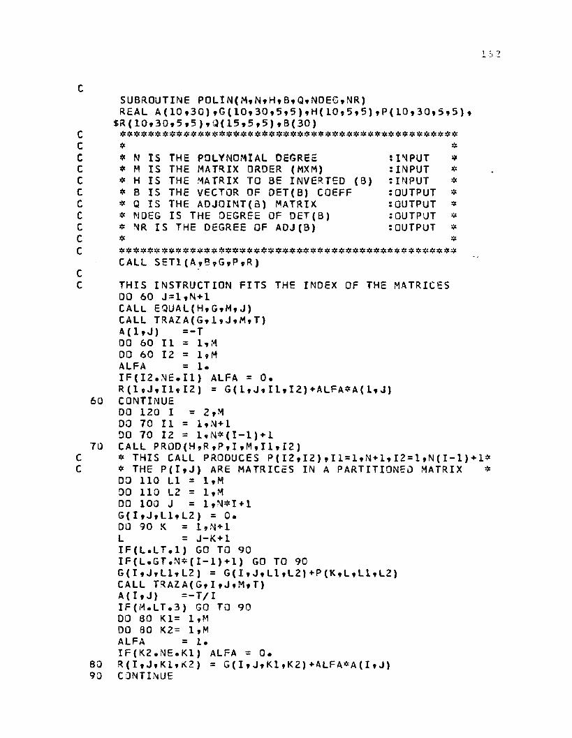
O o

oo

noononnnono

*? I NP UT: I NP UT *: I NP UT *: OUTPUT: OUTPUT: OUTPUT *1 OUTPUT *

SU B ROUTINE P O L l N ( M * N » H f B t Q * N D E G » N R )REAL A ( 1 0 , 3 0 ) » G ( 1 0 , 3 0 * 5 , 5 ) t H ( 1 0 ,5 « 5 ) ♦ P ( 1 0 9 3 0 , 5 9 5 ) *

$ R ( 1 0 » 3 0 * 5 * 5 ) » Q ( 1 5 * 5 » 5 ) * B ( 3 0 )

£♦ N I S THE POLYNOMI AL DEGREE♦ H IS THE MATRIX ORDER (MXM)♦ H I S THE MATRIX TO BE INVERTED (B)♦ B IS THE VE C T O R OF OET(B) COEFF♦ Q IS THE ADJ0INT(3) MATRIX♦ NOEG IS THE DEGREE OF DET(B)♦ NR IS THE DEG R E E OF ADJ(B)♦♦ # # # # # # # »Jc # # # # # # # # # # j!: 3* # a* ##3* * # 3* jjt 3*c # if ajt * ajt # # * # # * sjc 3* #3* # #CALL S E T I ( A , B , G , P » R )

THIS I N S T R U C T I O N FITS THE INDEX OF THE MATRICESDO 6 0 J = 1 , N + 1CALL E Q U A L ( H , G » M tJ)CALL T R A Z A ( G * l * J » M t T )A ( 1 *J ) =-T0 0 6 0 I I = I , M DO 6 0 1 2 = 1 » M ALFA = I .I F ( I 2 . N E . I 1 ) ALFA = 0 .R ( 1 1 J t I l f 1 2 ) = G ( I f I l f I 2 ) + A L F A * A ( I f J )

6 0 CONTI NUEDO 1 2 0 I = 2 fM DO 7 0 I I = I f N + l DO 7 0 1 2 = 1 9 N* ( I - 1 ) -*• 1

7 0 CALL P R 0 D ( H 9 R , P 9 l 9 M , I l , I 2 )♦ T H I S CALL PROOUCES P ( 1 2 9 1 2 ) 9 1 1 = 1 9 N + I f 1 2 = 1 f N ( 1 - 1 ) + 1 *♦ THE P ( I f J ) ARE MATRI CES I N A P A R T I T I ON E D MATRIX * DO 1 1 0 L I = 1 9 MDO 1 1 0 L2 = I 9 M DO 1 0 0 J = l f N ^ I + l G ( I 9 J 9 L i t L 2 ) = 0 .DO 9 0 X = IfN+lL = J-K+lIF(L.LT.l) GO TO 9 0 IF(L.GT.N* ( I - 1 ) + 1 ) GO TO 9 0 G(IfJfLl9L2) = G(IfJfLltL2 ) + P ( K 9 L 9 L l v L 2 )CALL T R A Z A ( G f I 9 J 9 M9 T)A ( I 9 J ) = - T / II F ( M . L T . 3 ) GO TO 9 0 DO 8 0 K1= l f M DO 8 0 K2= I 9 M ALFA = 1 .I F ( K 2 . N E . K 1 ) ALFA = 0 .

8 0 R(IfJfKl9K2) = G ( I f J tKl,K2)+ALFA*A(l9J)9 0 CONTI NUE

on

n o n o

100110120

1 3 0

1 4 0

1 5 0C

5 0 05 1 05 2 0

C

6 0 06 1 0

CONTI NUECONTI NUECONTI NUE$ 5** THE LAST BLOCK OF I N S T R U C T I O N S CALCULATE R ( I , J ) . F O R ** I=M* WE GET THE MATRI CES OF THE A D J ( H ) E XP ANS I ON ** *F = ( - l . ) * * ( M + l ) / MDO 1 3 0 K = 1 * N * M + 1 CALL T RA Z A( G* M* K» M» T )B ( K ) = F * T* 3 ( 1 ) ARE THE PARAMETERS I N THE EXP ANS I ON : ** O E T ( H ) = 3 ( l ) + B ( 2 ) * S + . . . + 3 ( N M + l ) * S * * N M I S I GN = ( - 1 ) * * ( M + 1 )I F ( I S I G N . E Q . - 1 ) T H E N 0 0 1 4 0 I = 1 * N * ( M - 1 ) +1 DO 1 4 0 J = 1 » M DO 1 4 0 K = l t M R ( M - l f I * J * K ) = —R ( M - 1 ? I * J t K)E NDI FDO 1 5 0 I = 1 ? N * ( M - l ) + 10 0 1 5 0 J = 1 *MDO 1 5 0 K = 1*MQ( T ♦ J* K) = R( M—1 » I » J » K )* F I L T E R FOR NR *NR = N * ( M - 1 )N1 = NRI F ( M . L T . 3 ) GO TO 5 2 0 DO 5 1 0 I = N l » l * - i DO 5 0 0 J = l t MDO 5 0 0 K = l t MI F ( A B S ( Q ( I + l » J , K ) ) * G T . l . E - 6 ) GO TO 5 2 0 CONTI NUENR = NR - 1CONTI NUE* F I L T E R FOR T AI L ZERO C O E F F I C I E N T S *NOEG = N*MCALL XMX I M( N D E G* B t X MX )N2 = NOEGDO 6 0 0 L = N 2 * l » - 1I F ( A B S ( f l ( L + l ) / X M X ) . G T . 3 . E - 3 ) GO TO 6 1 0NOEG = NOEG - 1CONTI NUECONTI NUERETURNEND

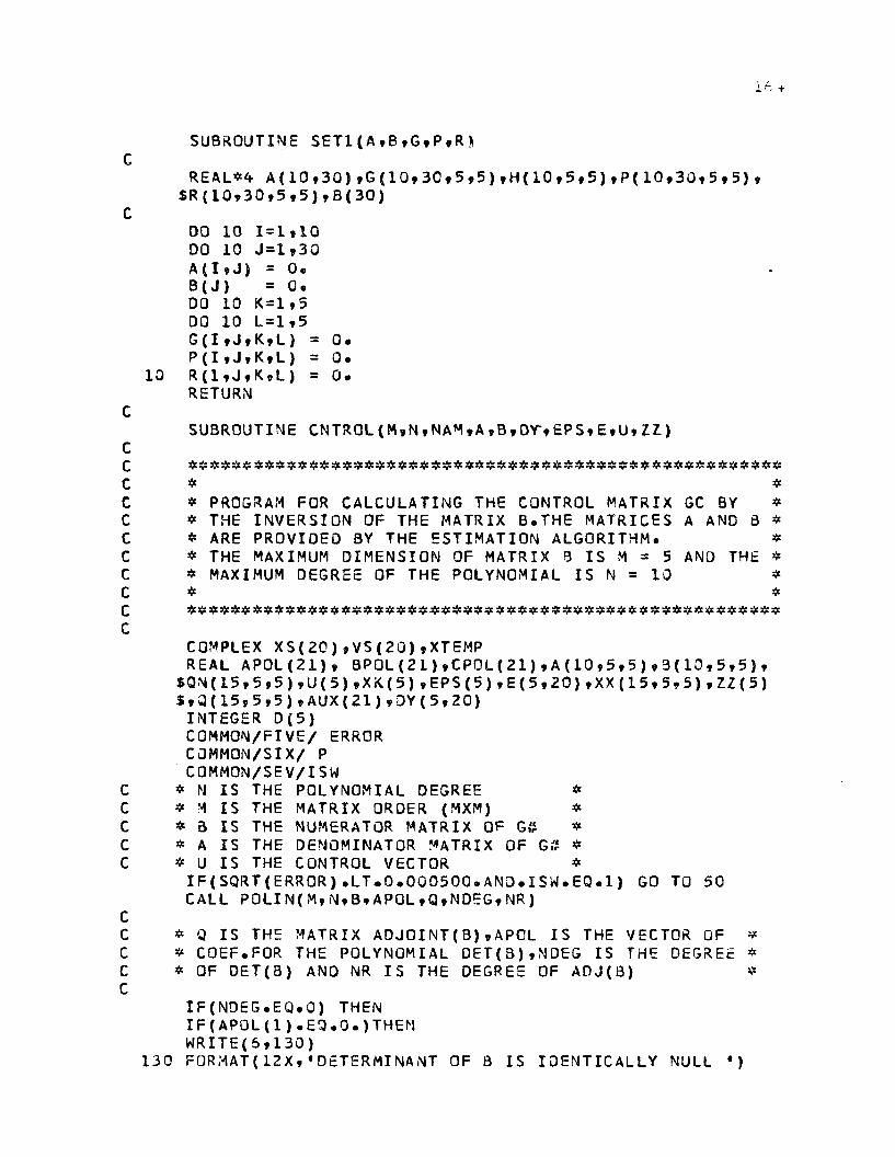
SUBROUTINE S E T 1 ( A , B , G , P , R )C

REAL*A A ( 1 0 , 3 0 ) » G ( 1 0 , 3 0 , 5 , 5 ) , H ( 1 0 , 5 » 5 ) , P ( 1 0 , 3 0 , 5 , 5 ) , $ R ( 1 Q , 3 0 » 5 , 5 ) » B ( 3 0 )

C00 10 1= 1,10 DO 1 0 J = 1 , 3 0 A ( I , J ) = 0 .3(J ) = 0.DO 1 0 K = 1 , 5 DO 1 0 L = 1 , 5 G (I«J,K,L) = 0.P ( I • J v K » L ) = 0 .

1 0 R ( 1 , J , K , L ) = 0 .RETURN

CSUBROUTI NE C N T R O L ( M , N , N A M , A , B , D Y > E P S , E , U ,11)

CC $$ fcsjcs* j*:### # j}e $£#####£ a*#### Jet#########*#:*##** $#####$: a*###*#C * *C * PROGRAM FOR CALCULATI NG THE CONTROL MATRI X GC BY *C * THE I N V E R S I O N OF THE MATRIX B . T H E MATRI CES A AND fl *C * ARE PROVI DED BY THE E S T I MA TI ON ALGORI THM. *C * THE MAXIMUM D I ME NS I ON OF MATRIX 3 I S M = 5 AND THE *C * MAXIMUM DEGREE OF THE POLYNOMIAL I S N = 1 0 *C * *C $jJcjfcaJc## jjt a*a*#### ####### ##$£#:*C

COMPLEX X S ( 2 0 ) , V S ( 2 0 ) , X T E M PREAL A P O L ( 2 1 ) , B P O L ( 2 1 ) , C P O L ( 2 1 ) , A ( 1 0 , 5 , 5 ) , 3 ( 1 0 , 5 , 5 ) ,

$ Q N ( 1 5 , 5 , 5 ) , U ( 5 ) , X K ( 5 ) , E P S ( 5 ) , E ( 5 , 2 0 ) , X X ( 1 5 , 5 , 5 ) , ZZ ( 5 ) $ , 3 ( 1 5 , 5 , 5 ) , A U X ( 2 1 ) , D Y ( 5 , 2 0 )

I NTEGER D C 5 )C OMMON / F I V E / ERROR COMMON / S I X / P CQMMON/ S EV/ I SW

c * N I S THE POLYNOMI AL DEGREE *c M I S THE MATRIX ORDER ( MXM) *c * B I S THE NUMERATOR MATRI X OF G# *c S* A I S THE DENOMINATOR MATRIX OF Gtf *c * U I S THE CONTROL VECTOR *

I F ( S Q R T ( E R R O R ) . L T . 0 . 0 0 0 5 0 0 . A N D . I S W . E Q . l ) GO TO 5 0 CALL P O L I N ( M» N , B , A P O L » Q * N D E G , N R )

CC * Q I S THE MATRIX A D J O I N T ( B ) , APOL I S THE VECTOR OF *C * COEF . F OR THE POLYNOMI AL D E T ( B ) , N D E G I S THE DEGREE *C * OF D E T ( B ) ANO NR I S THE DEGREE OF A D J ( 8 ) *C

I F ( N D E G . E Q . O ) THENI F ( A P Q L ( 1 ) . E Q . Q . ) T H E NW R I T E ( 5 » 1 3 0 )

1 3 0 FORMAT( 1 2 X , ‘ DETERMI NANT OF B I S I D E N T I C A L L Y NULL • )

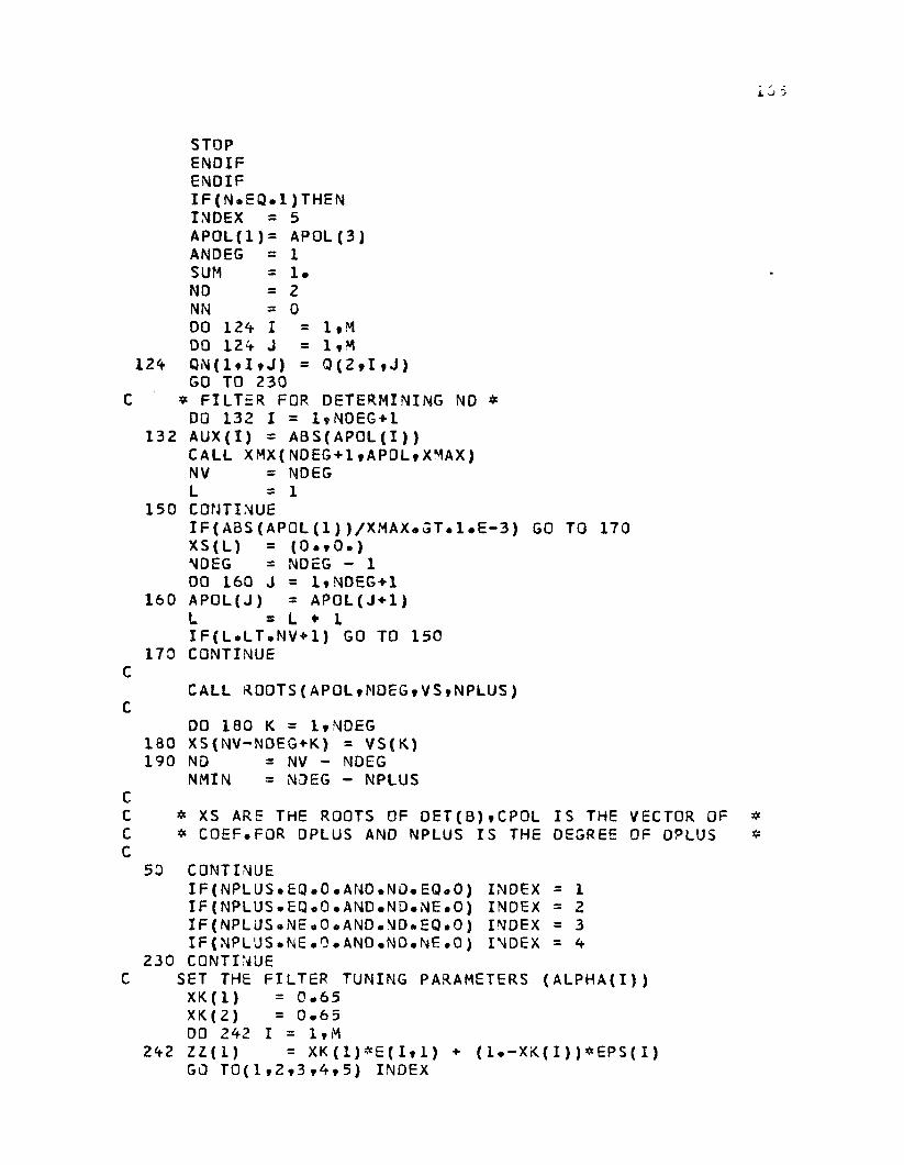
ODD

OSTOPE NDI FENDI FI F ( N * E Q . l J T H E N I NDEX = 5 AP O L ( 1 ) = A P O L ( 3 )ANDEG = 1 SUM = 1 .NO = 2NN = 0 DO 124- I = 1 *MDO 1 2 4 J = l f M

1 2 4 QN ( 1 9 1 9 J ) = Q ( 2 » I » J )GO TO 2 3 0

C * F I L T E R FOR DETERMI NI NG NO *DO 1 3 2 I = 1 » NOEG+1

1 3 2 A U X ( I ) = A 3 S ( A P O L ( I ) )CALL X M X { N D E G + I 9 AP O L 9 XMAX)NV = NDEGL = 1

1 5 0 CONTI NUEI F ( A B S ( A P 0 L ( 1 ) ) / X M A X . G T • 1 # E - 3 ) GO TO 1 7 0 X S ( L ) = ( O . 9 O . )NDEG = NDEG - 1 DO 1 6 0 J = I 9 NDEG+I

1 6 0 A P O L ( J ) = A P O L ( J + l )L « L ♦ II F ( L . L T . N V + 1 ) GO TO 1 5 0

1 7 0 CONTI NUE

CALL R 0 0 T S ( A P 0 L 9 N D E G 9 V S 9 N P L U S )

DO 1 8 0 K = 1 9 NDEG 1 8 0 XS ( NV - NDE G+ K) = V S ( K )1 9 0 ND = NV - NDEG

NMIN = NDEG - NPLUS

* XS ARE THE ROOTS OF D E T ( B ) 9 C P 0 L I S THE VECTOR OF* COE F . F OR DPLUS AND NPLUS I S THE DEGREE OF OPLUS

5 0 CONTI NUEI F ( N P L U S . E Q . O . A N O . N D . E Q . O ) I NDEX = 1I F ( N P L U S . E Q . O . A N D . N D . N E . O ) I NDEX = 2I F ( N P L U S » N E . O . A N D . N D * E Q . O ) I NDEX = 3I F ( N P L U S . N E . O * A N D . N D . N E . O ) I NDEX = 4

2 3 0 CONTI NUEC SET THE F I L T E R TUNI NG PARAMETERS ( A L P H A ( I ) )

XK ( 1 ) = 0 . 6 5XK( 2 ) = 0 . 6 5DO 2 4 2 I = I 9 M

2 4 2 11(1) = X K ( 1 ) * E ( I « 1 ) ♦ ( l . - X K ( I ) ) * E P S ( I )GO T 0 ( 1 , 2 t 3 f 4 9 5 ) I NDEX

1 5 6

1 NN = NRANDEG = 1 .SUM = 1 .CALL S E R V Q ( X X , Q , A , E P S , E , A P O L , N D E G , M , N N , N A M , D Y , U * Z Z , S U M

$ » ANDEG)GO TO 2 9 0

2 CALL D I A G ( M , N R , N D , Q , D )ANDEG = 1«SUM = 1 .CALL B M I N ( M , N R , N D , D , Q , Q N , N N )CALL S ERVQ( XX » QN, A , E P S t E * A P O L , N D E G , M , N N , N A M , D Y , U , Z Z ,

S S U M, A N D E G)GO TO 2 9 0

3 CALL C O E F ( V S , B P Q L * C P O L » N P L U S » N M I N )NN = NRSUM = 0®DO 2 5 0 I = 1 , N P L U S + 1

2 5 0 SUM = SUM ♦ C P O L ( I )ANDEG = A P O L ( N D E G + 1 )CALL S ERVO( XX , Q , A , E P S , E , B P O L , N M I N , M , N N , N A M , D Y , U , Z Z , S U M

$ , ANDEG)GO TO 2 9 0

4- CALL C O E F ( V S * BPOL » C P O L * N P L U S , N M I N )CALL D l A G ( M , N R , N D , Q , D )CALL 3 M I N ( M , N R , N D , D , Q , Q N » N N )SUM = 0 .DO 2 7 0 I = 1 , N P L U S + 1

2 7 0 SUM = SUM + C P O L ( I )ANDEG = A P O L ( N O E G + 1 )CALL S E R V O ( X X * Q N , A » E P S , E» BP OL» N M I N , M , N N , N A M , D Y , U , Z Z ,

S S UM, ANDEG)GO TO 2 9 0

5 CALL S E R V O ( X X , Q N * A , E P S , E » A P O L * N D E G , M , NN» NAM, DY * U , Z Z , S S U M, ANDE G)

3 3 0 CONTI NUE RETURN END

S UBROUTI NE S E T 2 ( Q , Q N , V S , X S )

COMPLEX X S ( 2 0 ) , V S ( 2 0 )REAL Q ( 1 5 , 5 , 5 ) , Q N ( 1 5 , 5 * 5 )DO 3 0 1 = 1 , 1 5 DO 3 0 J = 1 , 5 DO 3 0 K = 1 , 5 Q (I »J,K) = 0.

3 0 Q N ( I * J , K ) = 0 .DO 5 0 1 = 1 , 2 0V S ( I ) = C M P L X ( 0 . , 0 . )

5 0 X S ( I ) = C M P L X ( 0 . , 0 . )RETURNEND

o o n n o o

S UBROUTI NE S E R V O ( X X , G 1 *A , E P S , E , P O L »NDEG»M»NN»NAM » U D , U » $ Z Z , S U M, A D E G )

REAL G 1 ( 1 5 , 5 , 5 ) , A ( 1 0 * 5 * 5 ) , E P S ( 5 ) , E ( 5 * 2 0 ) , P O L ( 2 1 ) * U ( 5 ) * $ Z Z ( 5 ) , X X ( 1 5 , 5 , 5 ) , U D ( 5 , 2 0 ) , Y ( 5 )

s i c # # # # # # jJefcjJc ##:!Es4c:«c:4cj)e##:C£j!c5Sc<t $ •

* T H I S S UBROUTI NE CALCULATES THE CONTROL VECTOR U ** AS X = E P S + A 2 * E l + A 3 * E 2 + . . . + A N A M + l * E N A M ** AND P OL* U = X ** <e £ # # # # * * £ * * # # 5)e # # * :*£ J)e sje # ajt * j)c * # # « # # # # # # # # ❖ # * « * * * # * # # # *

CALL C L E A R ( X X )N*SkO;C = NN + . NAMCALL I DENT(M*1*XX*G1)DO 5 0 0 K = 1 * M DO 5 0 0 L = 1 * M DO 4 0 0 I = 2 , NC+ 1 X X ( I , K , L ) = G 1 ( I * K , L )I F ( I . G T . ( N N + 1 ) ) X X ( I , K , L ) = 0 .DQ 3 0 0 J = 1 , 1 - 1I F ( J , G T . N A M . O R « ( I - J ) . G T . ( N N + 1 ) ) G 0 TO 3 0 0 DO 3 0 0 1 1 = 1 , MX X ( I , K , L ) = X X ( I , K , L ) + G 1 ( I - J , K , I 1 ) * A ( J + 1 , I 1 , L )

3 0 0 CONTI NUE 4 0 0 CONTI NUE 5 0 0 CONTI NUE

I TYPE = 1 3I F ( I T Y P E . E Q . l ) THEN DO 4 5 0 L = 1 * NC + 1 W R I T E ( 6 , 4 2 0 ) L

4 2 0 F O R M A T ( / / 2 5 X , • G C ( • , I 1 , * ) * / / )DO 4 4 0 J = 1 , M

4 ^ 0 WRI T E ( 6 , 4 6 0 ) ( X X ( L , J , K ) , K = 1 , M)4 5 0 CONTI NUE4 6 0 F O R M A T ( / 2 0 X , 3 ( 2 X , F 1 2 * 4 ) / )

E NDI FCALL P R O M A T ( X X , E , Y , M , N C , Z Z )DO 2 0 I = 1 , MU ( I ) = Y ( I ) / ( A O E G * S U M )I F ( N O E G . G T . O ) THEN DO 1 0 J = 2 * NDEG+1

o o o

o ooooonon

C

1 0 U ( I ) = U ( I ) - P 0 L ( J ) * U D ( I , J + 9 )E NDI FU ( I ) = U ( I ) / P O L ( 1 )

2 0 CONTI NUE RETURN END:SUBROUTI NE B M I N ( M , N R , N O , D , Q , Q N , N )

s* 3*

* a.MIN AND DI AG CALCULATE THE PROOUCT OF MATRIX #* A D J ( B ) AND DI AGONAL MATRI X D I N OROER TO COMPENSATE ** THE MULTI PLE DELAYS *A *£ J * # # 5* 3*5* 3* 3* 3* 3* 5*3* 3* 5* # 3 * 3* # 5 * 3 * * 3 * $ 3 * 3* # 1 * 3 * 3* 3* # 3 * # 3 * 5 * $ # 2 * 3* 5* 3* 3* 3* 3* # 3 * * 3 *

REAL Q ( 1 5 , 5 , 5 ) , Q N ( 1 5 , 5 , 5 ) , Q E ( 1 5 , 5 > 5 , 5 ) , A L F A ( 1 5 )I NTEGER 0 ( 5 ) , DMAX

DO 5 0 0 I = 1 , 1 5 DO 5 0 0 J = 1 , 5 DO 5 0 0 K = 1 , 5 DO 5 0 0 L = 1 , 5

5 0 J Q E ( I , J , K , L ) = 0 .CALL XMAX( M» D, OMAX)DO 2 0 K = 1 » N R + 1 0 0 2 0 L = 1 , M DO 1 0 I = 1 , M DO 1 0 J = 1 , M A L F A ( L ) = 0 .I F ( J . E Q . L ) A L F A ( L ) = 1 .

1 0 Q E ( K , L , I , J ) = Q ( K , I , J ) * A L F A ( L )2 0 CONTI NUE

CALCULATI ON OF QN

N = NR+DMAX- NDDO 1 AO I = 1 , M DO 1 4 0 J = 1 , M DO 1 3 0 1 1 = 1 , N + 1 O N ( I I , I , J ) = 0 .DO 1 2 0 L = 1 , MK = NO - D ( L ) + I II F ( K » GT • N R + 1 ) GO TO 1 2 0Q N ( I l , I f J ) = Q N ( I 1 , I , J ) «• Q £ ( K , L , I , J )

1 2 0 CONTI NUE 1 3 0 CONTI NUE 1 4 0 CONTI NUE

RETURN END

A U X I L I A R PROGRAMS

17 G

SUBROUTINE OXAG( Mt Nt NO*0 *D)C

R E AL * 4 Q ( 1 5 , 5 » 5 ) , A U X ( I 0 )I NTEGER B ( 1 ) » 0 ( 1 ) , P ( 5 t 5 )

C * *C * M I S THE MATRIX ORDER *C * N I S THE POLYNOMI AL MATRI X DEGREE *C * ND I S THE GLOBAL DEAD TI ME A S S OC I A T E D WITH D E T ( B ) *C « Q I S THE MATRIX A Q J ( B ) *C * D I S THE MATRI CI AL PART OF B+ *C * XMAX CALCULATES THE MAXIMUM COMPONENT OF A VECTOR *C * ( I N T E G E R ) *C * XMX CALCULATES THE MAXIMUM COMPONENT OF A VECTOR *C * ( R E A L ) *C * *Q j*###############a*$ # # # # # $ $ £ « # # £ # # # # > ) £ £ i*##£s)es}t#sSei*jJc

DO 3 0 0 J = 1 * MDO 2 0 0 I = l t MP ( I » J ) = 1 0 0 0 DO 1 0 0 K = l t N + 1

1 0 0 AUX( K) = A 3 S ( Q ( K t I t J )CALL X M X ( N + l t A U X t Q M A X )DO 1 1 0 L = l t N + 1 I F ( A U X ( L ) / Q M A X . G T . 0 . 0 1 ) THEN P ( I t J ) = L - l GO TO 2 0 0 ENDI F

1 1 0 CONTI NUE 2 0 0 CONTI NUE

DO 2 2 0 1 1 = 1 tM 2 2 0 3 ( 1 1 ) = M A X ( O t N D - P ( l i t J ) )

CALL X M A X ( M f B t D ( J ) )3 0 0 CONTI NUE

RETURN END

CSUBROUTI NE S H I F T ( N 1 » N 2 t X t J t X l )

CREAL*4- X ( 5 t 2 0 )N3 = N 1 +1DO 1 0 I = N 2 * N 3 t - lX ( J , I ) = X ( J , I - 1 )

1 0 CONTI NUEX ( J t N l ) = XIRETURNEND

ooooooonooo

o n

oonnonoo

1 7 L

SUBROUTINE PRBS( N*X*PS)

10

REAL*“t PS =0 0 1 0 I = X ( I )CONTI NUE X ( N ) RETURN END

X ( N )= - X ( 1 ) * X ( N - 1 )

1 * N—1 = X (1+1)= PS

SUBROUTINE PROMAT{MATRIX,XINtXOUT,M,N,EPS)REAL MATRIX(15,5*5),XIN(5*20),X0UT(5),EPS{5)

# >Je Jjt # # # if. If. i/i & in # 3jc fc # £ # # # # £ # # # # :Jc :fc # j)e # ait # <e jje # # sjc * # fc # £ # * # $ $ # # :jc *

*****

T H I S S UBROUTI NE CALCULATES THE PRODUCT OF A REAL MATRIX M a Y A REAL VECTOR X I N G I V I N G THE PRODUCT VECTOR XOUT

$*#$*

♦ M A T R I X ( 1 , J , L ) * E P S ( L )

£ £ !jc 4c Jjc # & « jje # $ # # * # # # :£ # <: * $ # a?c # jjc$ * # £ jfc sjt 3je # * jjt £ # s* $ * # * J* sjc$ * # J(c $ £ £ *DO 1 0 0 J = l f MX O U T ( J ) = 0 *DO 1 0 0 L = 1 , M

1 0 0 X O U T ( J ) = X O U T ( J )I F ( N . G T . O ) THEN DO 2 0 0 I = 2 , N + 1DO 2 0 0 J = l t MDO 2 0 0 K = 1 * MX O U T ( J ) = X O U T ( J )

2 0 0 CONTI NUEWRI T E ( 6 , 1 9 9 ) ( J , X O U T ( J ) , J = 1 , M )

1 9 9 F O R M A T ( I X , ' F R O M PROMAT X 0 U T ( » , I 1 , » ) =E NDI F RETURN END

+ M A T R I X ( I , J , K ) * X I N ( K , I - 1 )

, 2 X , F 2 G . 5 )

SUBROUTI NE ROOT S ( 3 * N D E G , X S , N P L U S )

$ s)c * * Jjc if. * >* J* if « *c # # if * j* if * £ :* J* * <c $ <t 3j£ * # # £ * 5je # £ * * s* # «: # * # $ s)e * # s* # * sjt

* #* THI S PROGRAM I S AN IMPROVED VE R S I ON OF POLYROOT ** THE NUMBER OF I T E R A T I O N S ANO TOLERANCE ARE F I X E D ** THE ROOTS ARE FREE OF R E S I DUAL S AND THEY ARE ** ORDERED ACCORDI NG TO I N C R E A S I N G ABSOLUTE VALUE ** READY TO BE SEPARATED I NTO STABLE AND UNSTABLE ** S E T S . POLYROOT I S DUE TO D R . A . C O R R I P I O TO WHOM ** I AM VERY GRAT E F UL . *sje s)e £ a* # # * # * * >}: # # # # # * £ # j}t $ # * a* * * £ * J* # <e * « * # afte sjs * »c * 2 * * # # * #

COMPLEX X S ( 2 0 ) , XTEMPREAL D ( 2 0 ) * T E M P R , T E M P * C P 0 L ( 2 1 ) » B ( 2 1 )

CC

DO 8 I = 1 * 2 03 0 ( 1 ) = 0 .

1 0 CONTI NUEMAXI T = 6 5RTOL = 1 • E—6NC = NDEG + 1

CDO 2 0 1 = 1 , NDEG

2 0 X S ( I ) = ( 0 . , 0 . )CC EVALUATE ROOTS OF POLYNOMIAL BY MULLER• S METHODC

CALL XMULL( B , N D E G , X S , MAXI T, RTOL)DO 1 5 2 K = 1 »NDEGPR = R E A L C X S ( K ) )P I = A I M A G ( X S ( K ) )I F ( A 3 S ( P I J . L T . l . E - 5 ) THEN

C XTEMP = PRC X S ( K ) = XTEMP

X S ( K ) = C M P L X ( P R » 0 . )E NDI FI F ( A B S ( P R ) « L T e l s E —5 ) THEN X S ( K ) = C M P L X ( 0 . , P I )E NDI FI F ( A B S ( P R ) . L T . l . E - 5 . A N D . A 3 S ( P I ) . L T . l . E - 5 ) THEN XS (K.) = ( 0 . » 0 . )E NDI F

1 5 2 CONTI NUEDO 1 4 2 J = 1 , NDEG

1 4 2 D ( J ) = C A B S ( X S ( J ) )CALL 0 R D E R ( 0 » X S , N D E G , N P L U S )RETURNEND

CS UBROUTI NE XMULL( A , N , X S , MA X I T , RTOL )

CC PURPOSE - TO COMPUTE APPROXI MATI ONS OF THE ROOTS OFC NONLI NEAR EQUATI ONSCC RE F : CONTE AND OE BOOR, "ELEMENTARY NUMERI CAL A N A L Y S I S "C 3RD E D . , MCGRAW- HI LL, NEW YORK, 1 9 3 0 , P P . 1 2 0 - 1 2 7CC METHOD: MULLER• S METHOD OF QUADRATI C I NT E R P OL A T I ONCC VARI AB LE S I N ARGUMENT L I S TCC VARI ABLE TYPE I / O DI MENS I ON D E S C R I P T I O N

o o o

o o o

non

non

ooo

ooooooononnnnono

-y t

I I NUM3ER OF ROOTS TO BECOMPUTED

C I / O ARRAY CONTG. THE I N I T L . A P P R O X .AND RE T G. THE F I N A L VALUES

I I - m a x i m u m n u m b e r o f i t e r a t i o n s R I - r e l a t i v e e r r o r t o l e r a n c e

ON THE ROOTS E l - NAME OF S UBROUTI NE USED TO

EVALUATE THE F UNCTI ON

SUBPROGRAMS CALLEO

FUNCTN - TO EVALUATE THE NONLI NEAR F UNCTI ON DEFLAT - TO DEFLATE THE FUNCTI ON

COMPLEX X S { N ) * H , X , F X , F , D F P , F P , LAMBDA, D F , DFPL »C O E L T A , T O P , G , R A D , B Q T

REAL A ( 2 1 )

GUARD A G A I N S T ZERO OR NEGATI VE ERROR TOLERANCE

ETOL = A M A X 1 ( RTOL, l . E - 6 )

START OF LOOP TO EVALUATE N ROOTS

DO 1 0 0 I = 1 , N NEVAL = 0

EVALUATE AND DEFLATE FUNCTI ON AT F I R S T APPROXI MATI ON

1 0 H 0 . 5X = X S ( I ) *• HNEVAL = NEVAL ♦ 1CALL P O L Y ( A , N , X * FX )CALL D E F L A T ( I , X , FX* F , X S , I FLG )I F ( I F L G . N E . 0 ) GOTO 1 0

EVALUATE AND DEFLATE FUNCTI ON AT SECOND APPROXI MATI ON

DFP = F X = XS L I ) - HNEVAL = NEVAL + 1CALL P 0 L Y ( A * N * X , FX )CALL D E F L A T ( I , X , F X, F , X S , I F LG )I F ( I F L G . N E . 0 ) GOTO 1 0

I N I T I A L I Z A T I O N OF I T E R A T I V E CALCULATI ON

N

XS

MAXITRTOL

FUNCTN

FP = FDFP = FP - DFPX = X S ( I )

oo

no

on

o

n n

onn

no

on

LAMBDA = - 0 * 5 NEV = NEVAL + 1

I T E R A T I V E CALCULATI ON OF THE ROOT

0 0 3 0 NEVAL=NEV* MAX I T

CALL P O L Y ( A *N *X * FX )CALL D E F L A T ( I * X , F X » F» XS * I FLG )I F ( I F L G . N E . 0 ) GOTO 1 0

COMPUTE NEXT ESTI MATE OF ROOT

DF s F - FPDFPL = DFP * LAMBDA DELTA = 1 . ♦ LAMBDA TOP = - 2 . * F * DELTA

G = ( DELTA ♦ LAMBDA ) * DF - LAMBDA * DFPLRAO = C S Q R T ( G * * 2 + 2 . * T O P * L A M B D A * ( DF - D F P L ) )3 0 T = G + RADI F ( R E A L ( G ) * R E A L ( R A D ) + A T M A G ( G ) * A I M A G ( R A D ) . L T . 0 . )

BOT = G - RAD LAMBDA = TOPI F ( C A B S ( B O T ) . N E . 0 . ) LAMBDA = TOP / BOT

FP = F DFP = DFH = H # LAM3DAX = X + H

CHECK FOR CONVERGENCE

I F { C A B S ( H) . L T . ( ETOL * C A B S ( X ) ) ) GOTO 1 0 0

3 0 CONTI NUE

REACHED MAXIMUM NUMBER OF I T E R A T I ON S

WRI T E ( 6 * 1 1 0 ) NEVAL* I * X* FWRI TE( 4 , 1 1 0 ) NEVAL* I * X , F

1 1 0 FORMAT( / / l l X * * F A I L E D TO CONVERGE A F T E R * , 1 3 * I X ,&EVALUATI ONS * * * F 0 R ROOT• * I 3 / / 1 I X * • ROOT» « I P * 2 G 1 5 • 6£ , 5 X , * F ( R 0 0 T ) • , 2 G 1 5 . 6 )

C1 0 0 X S ( I ) = X

CRETURN

CEND

c*SUBROUTINE DEFLAT( I , X, FX, FDEF, XS , IFLG )

CC PURPOSE - TO DEFLATE THE FUNCTI ON F SO THAT THE SAMEC ROOT I S NOT ENCOUNTERED MORE THAN ONCECC VARI ABLES I N ARGUMENT L I S TCcr

VARI ABLE TYPE I / O DI MENS I ON D E S C R I P T I O N

c I I I NUMBER OF ROOT SOUGHTc X C I CURRENT APPROXI MATI ONc FX C I FUNCTI ON VALUE AT Xc FDEF C 0 DEFLATED VALUE AT Xc XS C I P REVI OUS ROOTS FOUNDc I FLG I 0 - FLAG SET TO ONE I F CURRENTcr

ROOT MATCHES P REVI OUS ROOTUr

COMPLEX X , F X , F D E F , X S ( 1 ) , BOTw

I F LG = 0FDEF = FX

rI F ( I . L T . 2 ) RETURN

VCr

DE F LATI ON OF F ( X )u

DO 1 0 K = 2 , IBOT X - X S ( K - l )I F ( C A B S ( B O T ) . L T . l c - 2 0 ) GOTO 2 010 FDEF = FDEF / BOT

rRETURNtc CURRENT APPROXI MATI ON MATCHES A ROOT. MODI FY ANO SETc I FLAG

2 0 X S ( I ) = X ♦ 0 . 0 0 1I F L G = 1RETURN

CEND

C*C*C*

S UBROUTI NE P O L Y ( A , N D E G , X » P )CC PURPOSE - TO EVALUATE A POLYNOMIAL OF NTH DEGREEC FOR SUBROUTI NE MULLERCC METHOD - NES TED MU L T I P L I C A T I O N ( S Y N T H E T I C D I V I S I O N )CC NDEG DEGREE OF THE POLYNOMIALC A ( N D E G + 1 ) C O E F F I C I E N T S OF THE POLYNOMIAL ORDEREDC I N AS CENDI NG POWERS OF X

ooooooooo

o on

n o

ooooooooo

1 ” 6

10

V AR I A B L E S I N ARGUMENT L I S T

VARI ABLE TYPE I / O D E S C R I P T I O N

X C

P C

COMPLEX X* P , 3 REAL A ( 2 1 )

NC = NOEG + 1 B = A ( N C )DO 1 0 1 * 1 * NDEG

K = NC - I B = B * X + A ( K)

P = B

I COMPLEX VALUE AT WHICH THEPOLYNOMI AL I S TO BE EVALUATED

0 COMPLEX VALUE OF THE POLYNOMIAL

RETURNEND

10

SUBROUTI NE I D E N T ( M* N * X* Y)

R E A L * * X ( 1 5 « 5 » 5 ) * Y ( l 5 » 5 t 5 )DO 1 0 I DO 1 0 J DO 1 0 K X ( I » J » K) CONTI NUE RETURN END

1 * N 1 * M 1 * MY ( I * K)

10

SUBROUTI NE C 0 E F ( X S » C * 3 t N P » N M )

£ * T H I S SUBROUTI NE CALCULATES THE C O E F F I C I E N T S FOR A POLYNOMI AL OF DEGREE N WHEN THE ROOTS ARE KNOWN ( N I S AN I NTERNAL PARAMETER>)

4c a* 4t 4c 4c & 4e if 4c 4: * # * 4c 4c 4e # 4e 4c Jjt # Sic # 4c 4« 4c # 4c * 4c * 4c # 4c 4c 4e 4e 4c4c 4s 4c 4c 4e ajt # 4c 4cCOMPLEX X S ( 2 0 ) * A ( 2 0 )REAL B ( 2 1 ) « C ( 2 1 )3 ( N P + 1 ) = 1 .C ( NM+1 ) = 1 .DO 1 0 I = 1 v 2 0 A ( I ) = ( 0 . * 0 . )A ( 1 ) = X S ( 1 )I F ( N P « E Q « 1 ) GO TO 1 0 0

DO 3 0 I = 2 f N P DO 2 0 J = I , Z r l

2 0 A ( J ) = A ( J ) + A ( J - 1 ) * X S ( I )3 0 A ( 1 ) = A ( 1 ) + X S ( I )

1 0 0 CONTI NUEDO 4 0 I * 1 *NP B ( N P + 1 - I ) = A ( I ) * ( - 1 ) * * I

4-0 CONTI NUEI F ( N M . E Q . C ) RETURN DO 1 1 0 I = 1 , 2 0

110 A (I) * (0*,0.)A ( 1 ) = X S ( 1 + N P )I F ( N M . E Q . l ) GO TO 2 0 0 DO 1 3 0 I = 2 * NM DO 1 2 0 J = I , 2 , - 1

1 2 0 A ( J ) s A ( J ) + A ( J - 1 ) * X S ( I + N P )1 3 0 A ( 1 ) = A ( 1 ) + X S ( I + N P )2 0 0 CONTI NUE

DO 14-0 I = 1 ? NN C ( N M + l - I ) = A ( I ) # ( —1 ) I

14-0 CONTI NUE C C (N M + 1 ) = 1.

RETURNEND

CSUBROUTI NE E Q U A L ( Y , X , M r L )

CREAL*4- X ( 1 0 , 3 0 , 5 , 5 ) , Y ( 1 0 , 5 , 5 )DO 1 0 I I = I , MDO 1 0 J 1 = 1 , MX ( 1 , L , 1 1 , J 1 ) = Y ( L , I 1 , J 1 )

1 0 CONTI NUERETURN END

CSUBROUTI NE T R A Z A ( X , I , J , M , T )

CR E A L * 4 X ( 1 0 , 3 0 , 5 , 5 )T = 0 .DO 1 0 L = 1 , N

1 0 T = T + X ( 1 , J , L , L )RETURNEND

CSUBROUTI NE P ROO( X , Y , P , I , M , 1 1 , 1 2 )

CREAL X ( 1 0 , 5 , 5 ) , Y ( 1 0 , 3 0 , 5 , 5 ) , P ( 1 0 , 3 0 , 5 , 5 )DO 1 0 L = 1 » M DO 1 0 J = 1 , M P ( I 1 , I 2 , L , J ) = 0 .DO 1 0 K = 1 , M

1 0 P ( I l , I 2 , L » J ) = P ( I 1 , I 2 » L , J ) + X ( I 1 , L , K ) * Y ( I - 1 , I 2 , K , J )

n n

x7;

c

c

c

c

RETURNEND

S UBROUTI NE ORDER( A t X S r N , N P L U S )COMPLEX X S ( 2 0 ) t CTEMP DI MENS I ON A ( 1 )DO 2 0 J = 1 * N - 1 I TEMP = JRMIN = A ( J )DO 1 0 I = J + 1 , N I F ( A ( I ) . L T . R M I N ) THEN RMIN * A ( I )I TEMP = IE N D I F

1 0 CONTI NUETEMP = A ( J )A ( J ) = RMINCTEMP = X S ( J )X S ( J ) = X S ( I TEMP )X S ( I TEMP) = CTEMP

2 0 A ( I T E M P ) = TEMPNPLUS = 0DO 3 0 I = l t N I F ( A ( I ) . G T . 1 . 0 0 ) GO TO 5 0 NPLUS = I

3 0 CONTI NUE 5 0 CONTI NUE

RETURN END

FUNCTI ON W N Q I S ( I S E E D f X M E A N v S D )

CALL R A N D U ( I S £ E D , I S E E D * P )WNOIS = ( P - Q . 5 ) * 2 . 0 * S D + X M E A NRETURNEND

SUBROUTI NE XMAX( Mf D * I MA X )

I NTEGER 0 ( 1 )T H I S SUBROUTI NE CALCULATES THE MAXIMUM COMPONENT OF A VECTOR D ( I N T E GE R VALUES )IMAX = A B S ( B ( 1 ) )I L A S T = 1 DO 1 0 0 I = 2 1 M I F ( A B S ( B ( I ) ) . G T . I M A X ) THEN IMAX = A B S ( B ( I ) )I L A S T = I ENDI F

1 0 0 CONTI NUE RETURN END

n n

179

CS UBROUTI NE XMX( M» B* XMAX)

CREAL 3 ( 1 )T H I S S UBROUTI NE CALCULATES THE MAXIMUM COMPONENT OF A VECTOR BXMAX = A B S ( B ( i ) )DO IOO I = 2 * M I F ( A B S ( B ( I ) ) . G T . X M A X ) THEN XMAX = A B S ( B ( I ) )ENOI F

- ? 1 0 0 CONTI NUE RETURN END

V I T A

Ivan P.Solar was born in Santiago,chile on April 30 1943.He completd his bachelor in Chfemical Engineering from Univ1 ersidad de Chile,Santiago in 1969 and obtained his master of science degree from Imperial College,University of London in 1975. he joined Universidad Catolica de Chile the year 1976. He is now a candidate for the degree of doctor in Philosophy in the department of Chemical Engineering at Louisiana State University.He is happily married to Isabel and they have a lovely daughter, Katia.He enjoys classic music,chess and astronomy.

180

Candidate:

Major Field:

Title o f Dissertation:

DOCTORAL EXAMINATION AND DISSERTATION REPORT

Ivan Patricio Solar

Chemical Engineering

Multivariable Adaptive Control Design Under Internal Model Control Structure

Approved:

M a jo r P r o f e s s o r a n d C h a i r m a n

J oD e a n o f t h e G r a d u a t e ^ S c h o o l

EXAMINING COMMITTEE:

C-xzLx.

_ _ S l (LyvN>>vv-|

Date of Examination:

February 17 . 1988