Multi­scale sensible heat fluxes in the urban environment from large aperture scintillometry and eddy covariance Article 

Accepted Version 

Ward, H. C., Evans, J. G. and Grimmond, C. S. B. (2014) Multi­scale sensible heat fluxes in the urban environment from large aperture scintillometry and eddy covariance. Boundary­Layer Meteorology, 152 (1). pp. 65­89. ISSN 0006­8314 doi: https://doi.org/10.1007/s10546­014­9916­4 Available at http://centaur.reading.ac.uk/36102/ 

It is advisable to refer to the publisher’s version if you intend to cite from the work.  See Guidance on citing  .

To link to this article DOI: http://dx.doi.org/10.1007/s10546­014­9916­4 

Publisher: Springer 

All outputs in CentAUR are protected by Intellectual Property Rights law, including copyright law. Copyright and IPR is retained by the creators or other copyright holders. Terms and conditions for use of this material are defined in the End User Agreement  . 

www.reading.ac.uk/centaur   

CentAUR 

Central Archive at the University of Reading 

Reading’s research outputs online

1

Multi-scale sensible heat fluxes in the suburban environment from 1

large aperture scintillometry and eddy covariance 2

H.C. Warda, b, J.G. Evansa, C.S.B. Grimmondb, c 3 4

a Centre for Ecology and Hydrology, Wallingford, Oxfordshire, OX10 8BB, UK 5 b Department of Geography, King’s College London, London, WC2R 2LS, UK 6 c Department of Meteorology, University of Reading, Reading, RG6 6BB, UK 7

Corresponding author email: helrda@ceh.ac.uk 8

9

Abstract 10

Sensible heat fluxes (QH) are determined using scintillometry and eddy covariance over a 11

suburban area. Two large aperture scintillometers provide spatially integrated fluxes across path 12

lengths of 2.8 km and 5.5 km over Swindon, UK. The shorter scintillometer path spans newly built 13

residential areas and has an approximate source area of 2-4 km2, whilst the long path extends from 14

the rural outskirts to the town centre and has a source area of around 5-10 km2. These large-scale 15

heat fluxes are compared with local-scale eddy covariance measurements. Clear seasonal trends are 16

revealed by the long duration of this dataset and variability in monthly QH is related to the 17

meteorological conditions. At shorter time scales the response of QH to solar radiation often gives 18

rise to close agreement between the measurements, but during times of rapidly changing cloud 19

cover spatial differences in the net radiation (Q*) coincide with greater differences between heat 20

fluxes. For clear days QH lags Q*, thus the ratio of QH to Q* increases throughout the day. In 21

summer the observed energy partitioning is related to the vegetation fraction through use of a 22

footprint model. The results demonstrate the value of scintillometry for integrating surface 23

heterogeneity and offer improved understanding of the influence of anthropogenic materials on 24

surface-atmosphere interactions. 25

Keywords 26

Energy balance; Large aperture scintillometer; Seasonality; Sensible heat flux; Urban 27

1. Introduction 28

Understanding the interactions between the land surface and the atmosphere is central to 29

developing our predictive power in terms of weather forecasting, air quality events, thermal 30

comfort, flood risk and tools for urban design. The surface energy balance has been closely linked to 31

land use and land cover, from studies both within and between cities. This has been achieved largely 32

2

through eddy covariance (EC) measurements at multiple sites in a city (e.g. in Los Angeles 33

(Grimmond et al. 1996), Basel (Christen and Vogt 2004), Łódź (Offerle et al. 2006), Melbourne 34

(Coutts et al. 2007), Montreal (Bergeron and Strachan 2010), Dublin (Keogh et al. 2012), Essen 35

(Weber and Kordowski 2010), Oberhausen (Goldbach and Kuttler 2013) and Helsinki (Nordbo et al. 36

2013)); and through comparison of measurements from different cities (e.g. Grimmond and Oke 37

(1995; 2002)). Also, studies at individual sites have combined footprint models and land cover maps 38

to capture differences in the surface cover sampled as the source area of the EC measurement 39

changes with atmospheric conditions (Vesala et al. 2008; Järvi et al. 2012; Goldbach and Kuttler 40

2013). The derived relations between surface cover and fluxes offer valuable indications of the 41

underlying processes and form a basis for modelling turbulent fluxes (Grimmond and Oke 2002; Järvi 42

et al. 2011; Loridan and Grimmond 2012). 43

Scintillometry provides a means to estimate fluxes at a much larger scale than eddy covariance, 44

typically of the order of several km2 (Hoedjes et al. 2007; Guyot et al. 2009; Kleissl et al. 2009a). 45

Path-averaging along the electromagnetic beam of the scintillometer means that measurements are 46

inherently spatially integrated, offering a particular advantage over heterogeneous surfaces (Beyrich 47

et al. 2002; Meijninger et al. 2002b; Evans 2009; Samain et al. 2011a). Despite the complexity of the 48

urban surface, patches of impervious land cover (roads, car parks, paved areas) adjacent to green 49

spaces (parks, gardens) are not very different to the juxtaposition of fields containing differently 50

ripening and senescing crops in mixed agricultural landscapes. In such studies, measuring sufficiently 51

high above the surface ensures the influences of surface heterogeneity are well-blended at the 52

height of the measurement and reliable fluxes can be obtained (Meijninger et al. 2002b; Ezzahar et 53

al. 2007). In addition to the increased spatial representativeness of such large-area measurements, 54

their increased scale facilitates comparison with satellite remote sensing products or land-surface 55

models. A key conclusion of the work by Chehbouni et al. (2000a) was that model development 56

should focus on establishing relations to replicate observations made at the large-scale. Studies 57

comparing model output with scintillometry data include the work of Cheinet et al. (2011), Samain 58

et al. (2011b), Steeneveld et al. (2011) and Maronga et al. (2013). 59

The use of scintillometers in urban environments can be divided into two groups: (a) studies 60

involving small aperture instruments, usually deployed within or near the top of the roughness sub-61

layer on path lengths of the order of 100 m, e.g. in Tokyo (Kanda et al. 2002), Basel (Roth et al. 2006) 62

and London (Pauscher 2010); and (b) studies over much longer path lengths (500 m - 10 km) using 63

large aperture scintillometers. This study uses large aperture scintillometry. The much larger 64

sampling volume enables robust retrieval of turbulence statistics and the measurement sensitivity is 65

3

greatest near the centre of the path, away from the instruments and their mounting structures, such 66

that the influence of locally-produced turbulence around these structures has minimal impact on the 67

measurements. Furthermore, direct access to the measurement area is not required – an 68

electromagnetic beam is simply transmitted high above the surface – unlike point measurements 69

requiring in situ mounting. This remote sensing capability makes the scintillometry technique 70

particularly valuable in the urban environment. 71

There are an increasing number of studies using large aperture scintillometry in urban areas. 72

Lagouarde et al. (2006) present results from a three week trial in summer 2001 in which two large 73

aperture scintillometers were used over Marseille. Other studies include work in London (Gouvea 74

and Grimmond 2010), Nantes (Mestayer et al. 2011), Łódź (Zieliński et al. 2012) and Helsinki (Wood 75

and Järvi 2012). 76

To date, the use of large aperture scintillometry in urban areas has been to derive the sensible 77

heat flux. In order to directly estimate the latent heat flux, a second scintillometer of longer 78

wavelength is required (Hill et al. 1988; Andreas 1989), however these are not yet commercially 79

available. Hence there are only a handful of two-wavelength studies documented (Kohsiek and 80

Herben 1983; Green et al. 2001; Meijninger et al. 2002a; Meijninger et al. 2006; Evans 2009). A 81

millimetre-wave scintillometer was installed alongside one of the infrared scintillometers used in this 82

study. These first two-wavelength results from the urban environment are presented in two 83

companion papers (Ward et al. in preparation a,b). 84

The goal of the work presented here is to investigate the influence of the surface on sensible 85

heat fluxes across different spatial and temporal scales in the suburban environment. Eddy 86

covariance measurements are analysed together with results from large aperture scintillometers 87

installed on 2.8 km and 5.5 km paths in Swindon, UK. The two year study period enables analysis of 88

seasonal and inter-annual patterns (Sect. 3.1) as well as the short-term response of heat fluxes to 89

solar radiation (Sect. 3.2). Consideration is given to the experimental uncertainties, including the 90

representativeness of point measurements required as inputs for scintillometry algorithms (Sect. 91

2.3) and the observational challenges associated with urban environments. The contributions of 92

different land cover classes are related to the observations at each scale by applying a footprint 93

model (Sect. 3.3). 94

4

2. Methodology 95

2.1. Derivation of the sensible heat flux from single-wavelength scintillometry 96

Scintillometers measure the intensity of an electromagnetic beam after propagation through the 97

turbulent atmosphere. Changes in beam intensity are related to the strength of turbulence and can 98

be converted to the structure parameter of the refractive index of air (Cn2). First, these refractive 99

index fluctuations must be related to temperature fluctuations, 100

2

2

22

n

T

T CA

TC , (1) 101

where CT2 is the temperature structure parameter and AT is the structure parameter coefficient 102

which depends on temperature (T), pressure (p) and weakly on humidity (Hill et al. 1980; Andreas 103

1988; Ward et al. 2013b). The Bowen ratio (β) correction given by Wesely (1976) (see Moene (2003) 104

for full details and a discussion) is not implemented in Equation 1 because β is not known a priori. 105

The effect of this is discussed in Sect. 2.3. 106

The conversion from structure parameters to fluxes entails iteration of similarity functions, fMO(ζ), 107

using Monin-Obukhov similarity theory (MOST) and the effective height of the scintillometer, zef, the 108

wind speed, U (which is measured at height zU), displacement height, zd, and aerodynamic 109

roughness length, z0. Commonly used forms of the similarity functions are 110

3/2

21 )1()( TTMO ccf (2) 111

for unstable conditions and 112

)1()( 3/2

31 TTMO ccf (3) 113

for stable conditions. The stability variable ζ is given by (zm-zd)/LOb, where LOb is the Obukhov length 114

and zm the measurement height, or zef/LOb when zef has been calculated incorporating the 115

displacement height (Hartogensis et al. 2003). Different values of the empirically derived constants 116

cT1-3 are used in the literature (Andreas 1988; Hill et al. 1992), and alternative functional forms 117

appear, e.g. Thiermann and Grassl (1992). The Wyngaard (1973) values were adjusted by Andreas 118

(1988) to give cT1 = 4.9, cT2 = 6.1 and cT3 = 2.2 (hereafter An88). De Bruin et al. (1993) found cT1 = 4.9, 119

cT2 = 9 and cT3 = 0 (hereafter DB93). These similarity functions relate the temperature structure 120

parameter to the temperature scaling variable (T*), 121

5

2/13/22

*)(

)(

MO

dmT

f

zzCT . (4) 122

The friction velocity, u*, is estimated from measured wind speed assuming a logarithmic wind profile 123

adjusted for stability and a value for the roughness length (e.g. Stull (1988)). The wind profile 124

equation is solved iteratively with 125

*

2

*

Tg

TuL

v

Ob , (5) 126

where g is the acceleration due to gravity and κv is the von Kármán constant (0.4). Note that this 127

equation for LOb neglects the buoyancy correction. Finally, the sensible heat flux is obtained using 128

**TucQ pH , (6) 129

where ρ is the density of air and cp the specific heat capacity at constant pressure. In the following, 130

QH_BLS and QH_LAS are used to denote the sensible heat flux for the 5.5 km path and 2.8 km path, 131

respectively (Sect. 2.2). The sensible heat flux from the EC station is denoted QH_EC. 132

One drawback of scintillometry is that the sign of the heat flux is unknown and must be assigned 133

based on other information. Following a comparison of possible algorithms, Samain et al. (2012) 134

recommended using an algorithm based on the minima in the diurnal cycle of Cn2 to indicate a 135

transition of stability. We follow a similar methodology here, which has the key advantage that it is 136

based on path-averaged information. 137

2.2. Site description and experimental details 138

This study took place in Swindon (population 175 000), situated 120 km west of London (top 139

right, Fig. 1). Typical of the UK suburban landscape, Swindon consists mainly of residential areas with 140

houses of varying ages extending outwards from the town centre, interspersed with greenspace, 141

small parades of shops and institutional buildings. Larger industrial and commercial zones are mostly 142

situated towards the edges of the development. The town centre comprises commercial areas, with 143

some pedestrianized streets, offices, public buildings and transport hubs. Building density in the 144

town centre is greater than in the surrounding suburbs and buildings are taller, larger and more 145

variable in height. Outside of the urban core the buildings are more uniform, houses are mostly 1-3 146

storeys, semi-detached or terraced and usually have at least a small garden. There are a few small 147

blocks of flats (4-5 storeys) and larger warehouses in industrial areas. Trees are of a similar height to 148

the buildings and found mostly in undeveloped green corridors between residential areas, along 149

6

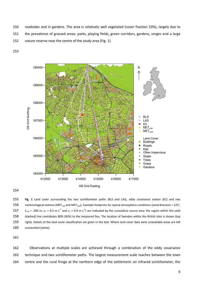
roadsides and in gardens. The area is relatively well vegetated (cover fraction 53%), largely due to 150

the prevalence of grassed areas: parks, playing fields, green corridors, gardens, verges and a large 151

nature reserve near the centre of the study area (Fig. 1). 152

153

154

Fig. 1 Land cover surrounding the two scintillometer paths (BLS and LAS), eddy covariance station (EC) and two 155

meteorological stations (METsub and METroof). Example footprints for typical atmospheric conditions (wind direction = 225°, 156

LOb = -200 m, u* = 0.5 m s-1 and σv = 0.9 m s-1) are indicated by the cumulative source area: the region within the solid 157

(dashed) line contributes 80% (95%) to the measured flux. The location of Swindon within the British Isles is shown (top 158

right). Details of the land cover classification are given in the text. Where land cover data were unavailable areas are left 159

unclassified (white). 160

161

Observations at multiple scales are achieved through a combination of the eddy covariance 162

technique and two scintillometer paths. The largest measurement scale reaches between the town 163

centre and the rural fringe at the northern edge of the settlement: an infrared scintillometer, the 164

7

BLS900 (Scintec, Rottenburg, Germany), was installed on a 5.5 km path orientated approximately 165

north-south. A second infrared scintillometer, a LAS 150 (Kipp and Zonen, Delft, The Netherlands), 166

was aligned on a shorter path of length 2.8 km. This path is located over relatively recently 167

developed suburbs (in the last 20 years or so) 3-5 km north of the town centre. Both are large 168

aperture scintillometers operating at a wavelength of 880 nm. Although LAS is an abbreviation for 169

large aperture scintillometer, in this study BLS is used to denote the scintillometer on the long path 170

and LAS the scintillometer on the short path. The EC system was installed approximately 3 km north 171

of the town centre, close to the middle of the long path. 172

Footprint models can be used to aid the interpretation of observed fluxes by relating them to the 173

probable area of the surface that influenced the measurements. Although some of the assumptions 174

may be challenged by complex environments, footprint models have been used successfully in urban 175

areas (Schmid et al. 1991; Järvi et al. 2009; Hiller et al. 2011), providing measurements are made at 176

sufficient height that the influences of individual obstacles or heterogeneities are averaged out. 177

Meijninger et al. (2002b) extended footprint theory to scintillometers by combining source areas 178

calculated for a single point measurement with the scintillometer path weighting function. This has 179

since been adopted by other studies (Meijninger et al. 2006; Hoedjes et al. 2007; Samain et al. 180

2011a; Evans et al. 2012; Liu et al. 2013). A range of footprint models exist; here we use the 181

analytical model of Hsieh et al. (2000) and assume the lateral dispersion is Gaussian (Schmid 1994; 182

Detto et al. 2006). 183

Results of the footprint model for each of the three systems are shown in Fig. 1 for typical 184

atmospheric conditions (wind direction = 225°, LOb = -200 m, u* = 0.5 m s-1 and standard deviation of 185

lateral wind σv = 0.9 m s-1). Source areas vary depending on atmospheric conditions and wind 186

direction, as well as measurement height and surface roughness. The difference in measurement 187

scales is apparent. The sizes of the areas contributing 80% (95%) of the observed fluxes are 188

approximately 0.06, 1.0 and 3.0 km2 (0.5, 3.0 and 7.5 km2) for the EC, LAS and BLS, respectively. The 189

size of the footprints increases with stability. 190

Beam heights, land cover and building and tree height were obtained using a spatial database 191

incorporating surface cover information (OS MasterMap 2010 ©Crown Copyright), a digital terrain 192

model and digital surface model from lidar (2007, ©Infoterra Ltd) and aerial photography (2009, 193

©GeoPerspectives). For this study a spatial resolution of 5 m was used, further details are given in 194

Ward et al. (2013a). Some of the residential area at the far north-west of the study area has very 195

recently been completed, with some ongoing development of the rural outskirts during the study 196

period. The overall effect here may be a small overestimation of the vegetated land cover fraction 197

8

for the LAS path, when winds are from the west or north-west and in stable conditions, as this recent 198

development has not yet been incorporated in the spatial database. 199

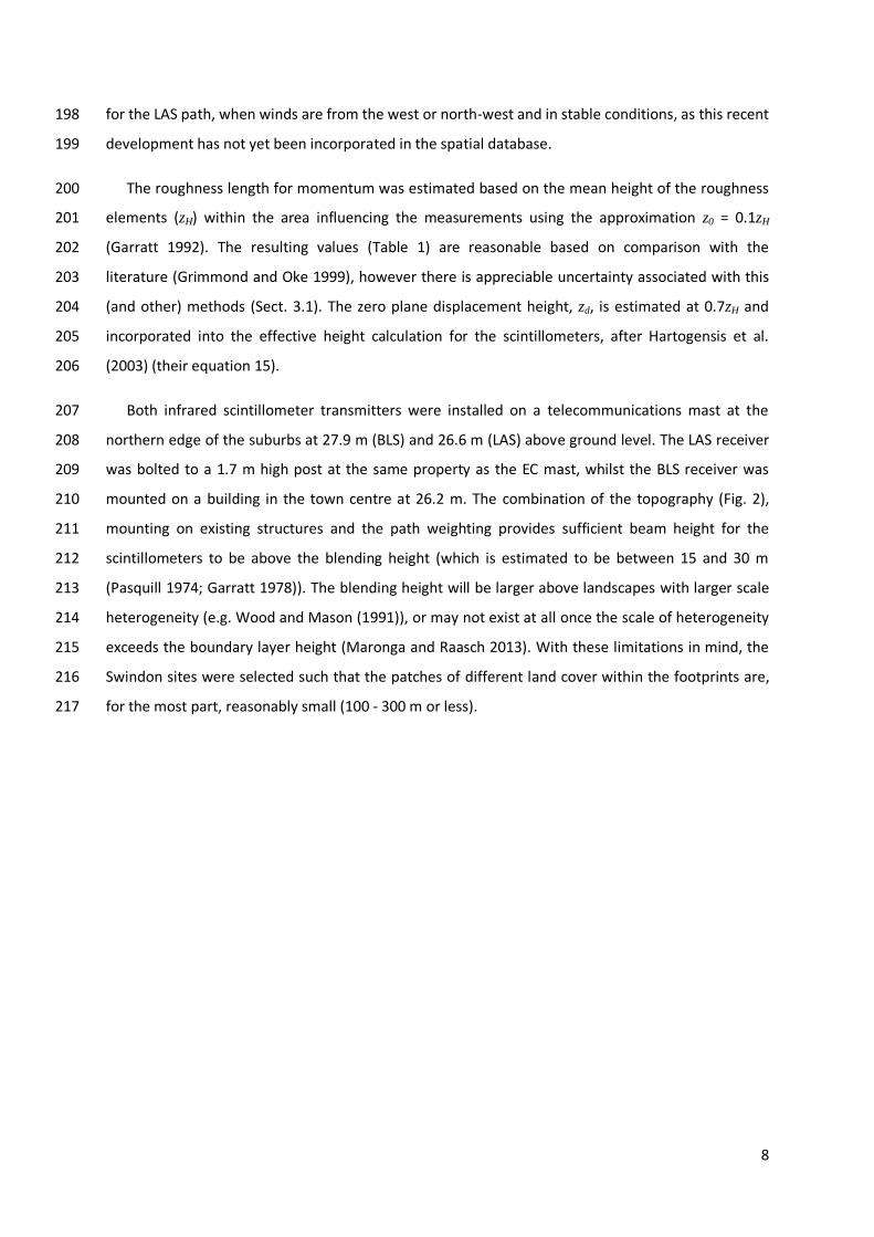
The roughness length for momentum was estimated based on the mean height of the roughness 200

elements (zH) within the area influencing the measurements using the approximation z0 = 0.1zH 201

(Garratt 1992). The resulting values (Table 1) are reasonable based on comparison with the 202

literature (Grimmond and Oke 1999), however there is appreciable uncertainty associated with this 203

(and other) methods (Sect. 3.1). The zero plane displacement height, zd, is estimated at 0.7zH and 204

incorporated into the effective height calculation for the scintillometers, after Hartogensis et al. 205

(2003) (their equation 15). 206

Both infrared scintillometer transmitters were installed on a telecommunications mast at the 207

northern edge of the suburbs at 27.9 m (BLS) and 26.6 m (LAS) above ground level. The LAS receiver 208

was bolted to a 1.7 m high post at the same property as the EC mast, whilst the BLS receiver was 209

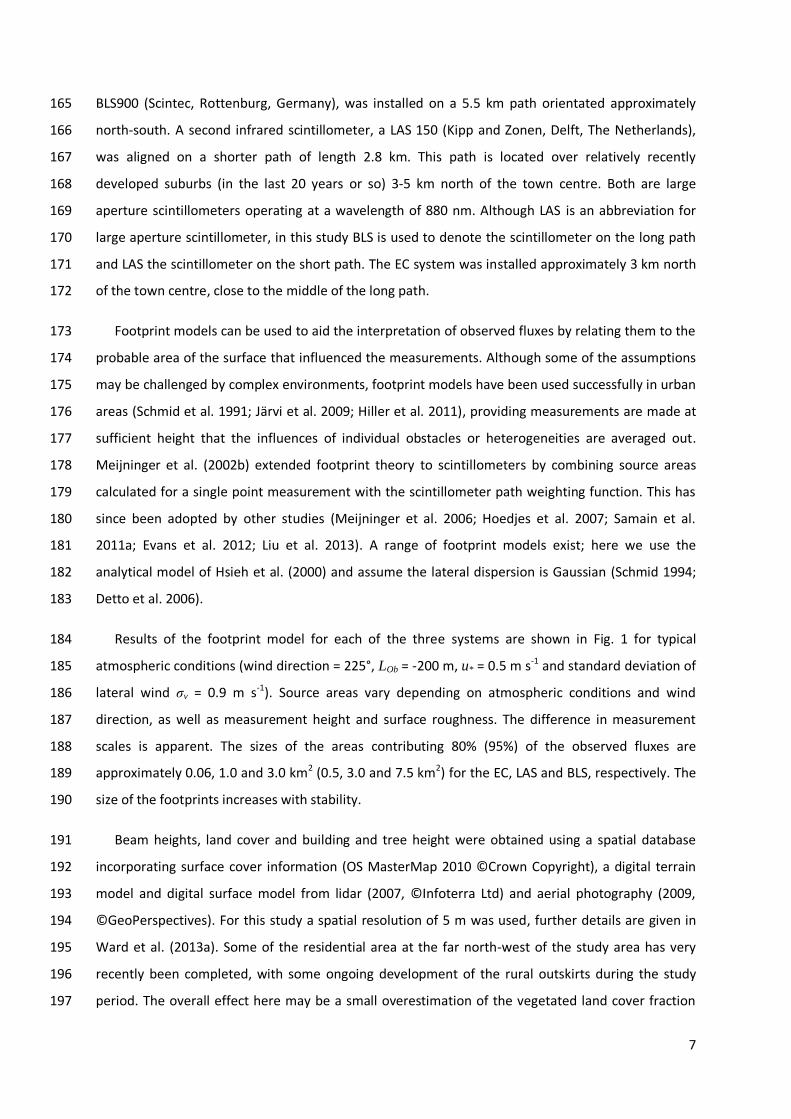
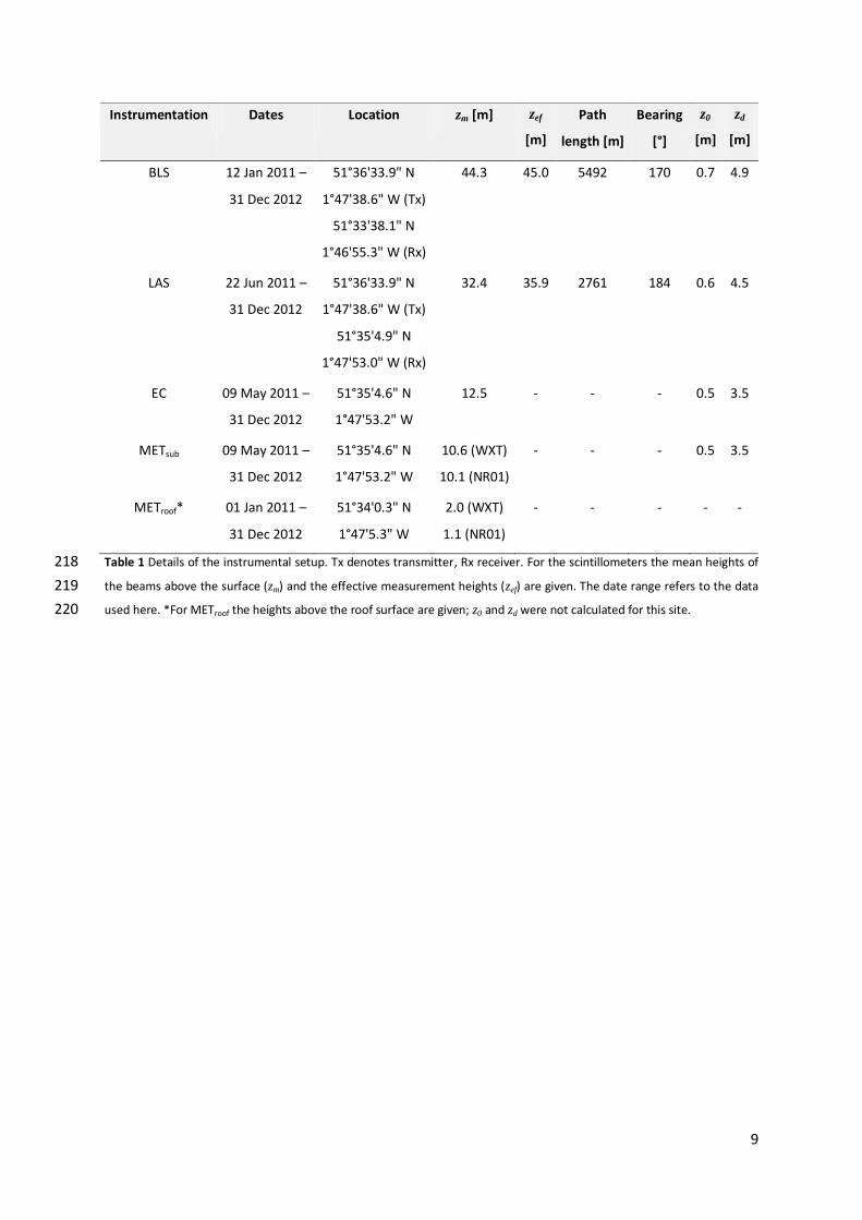
mounted on a building in the town centre at 26.2 m. The combination of the topography (Fig. 2), 210

mounting on existing structures and the path weighting provides sufficient beam height for the 211

scintillometers to be above the blending height (which is estimated to be between 15 and 30 m 212

(Pasquill 1974; Garratt 1978)). The blending height will be larger above landscapes with larger scale 213

heterogeneity (e.g. Wood and Mason (1991)), or may not exist at all once the scale of heterogeneity 214

exceeds the boundary layer height (Maronga and Raasch 2013). With these limitations in mind, the 215

Swindon sites were selected such that the patches of different land cover within the footprints are, 216

for the most part, reasonably small (100 - 300 m or less). 217

9

Instrumentation Dates Location zm [m] zef

[m]

Path

length [m]

Bearing

[°]

z0

[m]

zd

[m]

BLS 12 Jan 2011 –

31 Dec 2012

51°36'33.9" N

1°47'38.6" W (Tx)

51°33'38.1" N

1°46'55.3" W (Rx)

44.3

45.0 5492 170 0.7 4.9

LAS 22 Jun 2011 –

31 Dec 2012

51°36'33.9" N

1°47'38.6" W (Tx)

51°35'4.9" N

1°47'53.0" W (Rx)

32.4 35.9 2761 184 0.6 4.5

EC 09 May 2011 –

31 Dec 2012

51°35'4.6" N

1°47'53.2" W

12.5 - - - 0.5 3.5

METsub 09 May 2011 –

31 Dec 2012

51°35'4.6" N

1°47'53.2" W

10.6 (WXT)

10.1 (NR01)

- - - 0.5 3.5

METroof* 01 Jan 2011 –

31 Dec 2012

51°34'0.3" N

1°47'5.3" W

2.0 (WXT)

1.1 (NR01)

- - - - -

Table 1 Details of the instrumental setup. Tx denotes transmitter, Rx receiver. For the scintillometers the mean heights of 218

the beams above the surface (zm) and the effective measurement heights (zef) are given. The date range refers to the data 219

used here. *For METroof the heights above the roof surface are given; z0 and zd were not calculated for this site. 220

10

221

Fig. 2 Cross section of the topography (solid black line) and mean obstacle height (dotted line; buildings and trees within a 222

radius of 100 m) along the (a) BLS and (b) LAS paths (coloured lines). 223

224

A CR5000 datalogger (Campbell Scientific Ltd., Loughborough, UK) sampled the intensity of the 225

received LAS beam at 500 Hz and measured the Cn2 signal (calculated onboard the instrument and 226

stored as a logarithm) every second which was then output at 1 min intervals and these were 227

averaged to 10 min. For the BLS, the mean and standard deviation of the beam intensity of each disk 228

(the BLS900 is a dual disk instrument with two transmitting apertures) were obtained from the 229

supplied signal processing unit at 30 s intervals, then converted to log-amplitude variances and Cn2 230

and averaged up to 10 min. Data from a single disk are presented here. 231

The EC system consists of a sonic anemometer (R3, Gill Instruments Ltd., Lymington, UK) and an 232

open-path infrared gas analyser (LI-7500, LI-COR Biosciences, Lincoln, USA) at a height of 12.5 m. As 233

this is 2-3 times the height of the surrounding buildings and trees, it is therefore sufficiently high to 234

deliver fluxes representative of the local-scale. Data were processed using EddyPro (LI-COR) 235

11

following conventional procedures. Further details of the EC measurements can be found in Ward et 236

al. (2013a). 237

Meteorological instruments were installed on the same mast as the EC equipment (denoted 238

METsub). A second set of meteorological data were collected at a rooftop site close to the town 239

centre (METroof). Both stations included a four-component radiometer (NR01, Hukseflux, Delft, The 240

Netherlands), automatic weather station (WXT510, Vaisala, Helsinki, Finland) and tipping bucket rain 241

gauge (0.2 mm tip, Casella CEL, Bedford, UK). At METsub, the radiometer was installed at a height of 242

10.1 m so that the downward-facing field of view comprises a mixture of surfaces: grass lawns and 243

verges, road, pavement, hedges and small trees, bare soil, gravel, roofs of garages, small sheds and 244

single-storey extensions and walls (brick and painted). At METroof, the radiometer was installed at 1.1 245

m above the roof surface made of grey synthetic material and black rubber matting. Additionally at 246

METroof, a heat flux plate (HFP01, Hukseflux) was installed between the roof surface and rubber 247

sheet, providing an approximation of the change in storage through the roof. At both sites the 248

meteorological data were logged at 1 min intervals (CR1000, Campbell Scientific Ltd.) and 249

subsequently averaged to obtain 10 min resolution for calculation of the scintillometer fluxes or 30 250

min for comparison with EC fluxes. The 10 min scintillometer fluxes were also averaged to 30 min for 251

comparison with EC results. Details of the observational setup are summarized in Table 1. 252

To provide nearly continuous auxiliary data required for scintillometry processing, results from 253

the two meteorological stations were combined. When available, data from METsub are used as the 254

siting of this station is more appropriate. Based on the regression of concurrent data (9 May 2011 - 255

31 Dec 2012), temperature, relative humidity (RH), pressure and wind speed at METroof were 256

adjusted to gap-fill the combined dataset, including the period prior to installation of METsub on 9th 257

May 2011. This is considered further in Sect. 2.3. 258

All data were subject to quality control routines. Data were removed at times of known 259

instrument malfunction. Meteorological data were excluded when they (or their standard 260

deviations) fell outside physically reasonable thresholds. Quality control of the scintillometry data 261

included rejecting times when the received signal intensity dropped below half of the value in clear 262

conditions, which usually indicated rain or fog. Data points neighbouring those that failed the 263

intensity check were also removed. Out of the total data collected, 84% of BLS and 82% of LAS data 264

(10 min) remained for analysis. 265

Both scintillometers were corrected for the effects of saturation using the modulation transfer 266

function of Clifford et al. (1974). Using the threshold value suggested by Kleissl et al. (2010), 16% of 267

12

the BLS data and 0.2% of the LAS data might be expected to suffer from saturation. Overall, the 268

correction increased Cn2 by 4% and 1% for the BLS and LAS respectively (naturally the corrections are 269

larger with increased scintillation and rise to 8% and 2% for the midday periods). 270

Recent studies have indicated sometimes severe discrepancies between certain scintillometers, 271

in particular the LAS 150 model (Kleissl et al. 2008), whereas the BLS900 model tends to give more 272

reproducible results (Kleissl et al. 2009b). Prior to deployment in Swindon, the LAS and BLS were run 273

alongside each other at a fairly homogenous grass test site at Chilbolton Observatory, Hampshire, 274

UK (17 April 2010 – 25 May 2010). Observed Cn2 ranged between 10-16 m-2/3 and 10-12 m-2/3, which 275

spans the range of values observed for the Swindon paths. Results suggested the response of the 276

LAS is reasonable but compared to the BLS Cn2 is overestimated by 9.8%. This adjustment has been 277

applied to the LAS Cn2 for the Swindon data. As a result of these comparisons (e.g. Kleissl et al. 278

(2008; 2009b), Van Kesteren and Hartogensis (2011)), Kipp and Zonen have updated their original 279

LAS 150 instrument to a LAS MkII model (Mustchin et al. 2013). 280

2.3. Assessment of the input meteorological data 281

First, the suitability of the combined meteorological input data used to process the scintillometry 282

fluxes is considered. To calculate QH from single-wavelength scintillometry, air temperature, 283

pressure and humidity are required to first obtain the structure parameter of temperature, CT2. Both 284

T and RH are similar between the METsub and unadjusted METroof sites. The regression slopes are 285

within 3% and there is high correlation (r2 > 0.98). Sensitivity of QH to these input meteorological 286

variables is small (Hartogensis et al. 2003) and indeed these very small differences have minimal 287

impact on the fluxes. The average difference in QH is < 0.5% when calculated using T, RH and p from 288

each site. Use of this combined dataset is therefore judged unproblematic and to be a sufficiently 289

accurate representation of T, RH and p across the study area. 290

An initial estimate of the Bowen ratio is recommended to account for the contribution of 291

humidity and combined temperature-humidity fluctuations to optical Cn2 (Wesely 1976). Usually the 292

value of β is arrived at iteratively through incorporation of the available energy (e.g. Meijninger et al. 293

(2002b)). However, estimating the available energy is challenging in urban areas as the net storage 294

heat flux (ΔQS) plays a more significant role in the energy balance than for most rural areas (e.g. 295

grassed or agricultural land), yet it is very difficult to measure directly (Offerle et al. 2005; Roberts et 296

al. 2006). Other (rural) studies have used β measured at a nearby station (Hoedjes et al. 2002; 297

Samain et al. 2011a) or have calculated QH using a series of values of β (Meijninger and De Bruin 298

2000). When β is expected to be large (e.g. > 0.6 for Chehbouni et al. (2000b); > 1 for Moene (2003)) 299

13

the correction may be neglected. Given the uncertainty in estimating the available energy and the 300

lack of representative EC data across the whole study area, the Bowen ratio correction has not been 301

applied for the results presented here. The potential impact is an average overestimation in QH from 302

the scintillometers of less than 5% for β > 1, and less than 10% for β = 0.5. For the BLS, the CT2 values 303

here were found to be within around 6% of the CT2 values calculated incorporating data from the 304

millimetre-wave scintillometer (Sect. 1), which do not require a Bowen ratio correction (see Ward et 305

al. (in preparation b) for details). 306

To process scintillometry data, the friction velocity is usually estimated from wind speed 307

measured at a single point and adjusted to beam height using the logarithmic profile accounting for 308

stability. As with the other meteorological inputs, wind speed from METroof was adjusted to produce 309

the combined dataset with optimum availability of input data. Concurrent QH values calculated using 310

the METsub wind speed or the adjusted METroof wind speed differ by less than 3%, r2 is high (0.98) and 311

there is little scatter (root mean squared error, RMSE < 10 W m-2). 312

The dual-disk design of the BLS900 enables estimation of the path-averaged crosswind, i.e. the 313

component of the wind speed perpendicular to the scintillometer path. To check that the point 314

measurements of wind speed were a realistic proxy for the wind field over the scintillometer source 315

area, a comparison was made between the BLS crosswind speed and the equivalent crosswind speed 316

calculated using wind speed and direction from METsub and scaled to the effective height of the BLS 317

using stability from the EC station. Overall the crosswind estimates displayed similar trends across a 318

range of wind speeds and directions. The high correlation obtained (r2 = 0.922) implies that these 319

point measurements generally capture the variability of the wind field at the larger scale and gives 320

confidence in their use in processing the scintillometry data. 321

3. Analysis of sensible heat fluxes 322

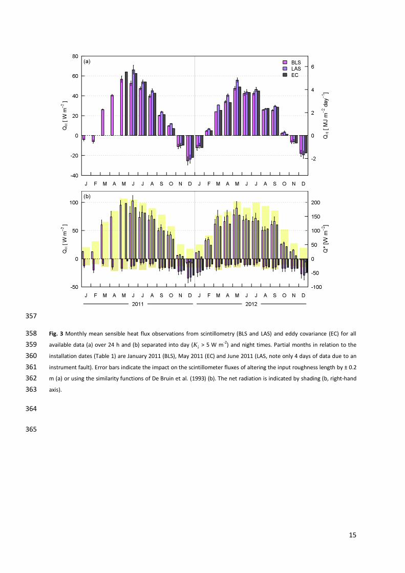
3.1. Assessment of seasonal cycles and annual variations 323

Large-area sensible heat fluxes from the 5.5 km scintillometer path are presented for two years 324

(2011-12), alongside 18 months of data from the shorter 2.8 km scintillometer path and almost 20 325

months of eddy covariance data (Fig. 3). The annual cycle is evident, with mean daily (24 h) QH 326

reaching a maximum in early summer (May-June in 2011, May in 2012) and minimum in December. 327

In December, average QH is negative even during daytime (defined as times when incoming 328

shortwave radiation K↓ > 5 W m-2, see Fig. 3b) as the typical diurnal course of QH becomes positive 329

only for a few hours around midday (Fig. 4). This behaviour is observed consistently across the three 330

datasets and in both years but contrasts with the majority of urban studies in more built-up areas, 331

14

where greater heat release from storage and anthropogenic activity can maintain a positive sensible 332

heat flux all year round (Offerle et al. 2005; Kotthaus and Grimmond in press-a). For two sites in 333

Oberhausen, Germany, Goldbach and Kuttler (2013) found QH to be positive for most of the daytime 334

throughout the year at their urban site, whereas their suburban site exhibits similar behaviour to 335

Swindon. Besides the smaller storage and anthropogenic heat flux in suburban areas, more of the 336

available energy is partitioned into evaporation, owing to increased moisture availability from soil 337

surfaces and greater total evapotranspiration from a larger vegetation fraction. 338

Within the trends of the expected annual cycle, there are notable differences between the two 339

years studied. Peak QH is larger in summer 2011 compared to 2012 and month-to-month variation is 340

smaller in 2011. Broadly speaking, much of 2011 was under threat of drought, with dry soil moisture 341

conditions and depleted ground water supplies. Despite frequent rain and very few clear sky days 342

the annual rainfall total was 530 mm compared to the average 780 mm for southern England1. Dry 343

conditions continued through early spring 2012, until early April. Very wet weather followed and 344

remained throughout 2012 (total rainfall 1020 mm), with brief drier and warmer spells in late July 345

and early September. 346

June 2012 was particularly wet and cloudy (sunshine hours were only 70% of normal1; mean 347

daytime K↓ was 174 W m-2 in 2012 compared to 212 W m-2 in 2011). Monthly mean daily QH was 348

19%, 34% and 31% lower than in June 2011 for the BLS, LAS and EC, respectively. August 2012 also 349

had a notably lower QH during daytime compared to 2011 (also shown in Fig. 4), despite similar 350

radiative energy inputs in both years. A long dry spell and generally sunny weather in September 351

2012 allowed surfaces to dry out and QH to increase, resulting in a larger average value than for the 352

previous month. Large negative nocturnal QH_BLS in February 2011 means the daily (24 h) average is 353

negative, whereas high Q* and high daytime QH_BLS in 2012 contribute to a positive 24h average in 354

2012 (Fig. 3). 355

356

1 Met Office climate statistics (1971-2000), http://www.metoffice.gov.uk/climate, last accessed 29 March 2013

15

357

Fig. 3 Monthly mean sensible heat flux observations from scintillometry (BLS and LAS) and eddy covariance (EC) for all 358

available data (a) over 24 h and (b) separated into day (K↓ > 5 W m-2) and night times. Partial months in relation to the 359

installation dates (Table 1) are January 2011 (BLS), May 2011 (EC) and June 2011 (LAS, note only 4 days of data due to an 360

instrument fault). Error bars indicate the impact on the scintillometer fluxes of altering the input roughness length by ± 0.2 361

m (a) or using the similarity functions of De Bruin et al. (1993) (b). The net radiation is indicated by shading (b, right-hand 362

axis). 363

364

365

16

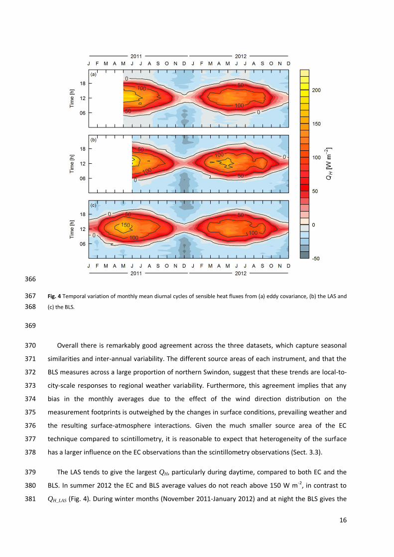
366

Fig. 4 Temporal variation of monthly mean diurnal cycles of sensible heat fluxes from (a) eddy covariance, (b) the LAS and 367

(c) the BLS. 368

369

Overall there is remarkably good agreement across the three datasets, which capture seasonal 370

similarities and inter-annual variability. The different source areas of each instrument, and that the 371

BLS measures across a large proportion of northern Swindon, suggest that these trends are local-to-372

city-scale responses to regional weather variability. Furthermore, this agreement implies that any 373

bias in the monthly averages due to the effect of the wind direction distribution on the 374

measurement footprints is outweighed by the changes in surface conditions, prevailing weather and 375

the resulting surface-atmosphere interactions. Given the much smaller source area of the EC 376

technique compared to scintillometry, it is reasonable to expect that heterogeneity of the surface 377

has a larger influence on the EC observations than the scintillometry observations (Sect. 3.3). 378

The LAS tends to give the largest QH, particularly during daytime, compared to both EC and the 379

BLS. In summer 2012 the EC and BLS average values do not reach above 150 W m-2, in contrast to 380

QH_LAS (Fig. 4). During winter months (November 2011-January 2012) and at night the BLS gives the 381

17

largest fluxes. Daily average QH_EC often lies between the two scintillometer averages but during 382

winter (November-December 2011, December 2012) and at night the scintillometers tend to give 383

larger magnitude QH. This can also be seen in Fig. 4: the absolute size of QH from the scintillometers 384

is larger (e.g. around transition times in December), whether positive or negative, whereas EC values 385

are much closer to zero. Larger scintillometer fluxes in neutral-to-stable conditions may reflect the 386

performance of the similarity functions (Sect. 3.2). 387

The widely implemented similarity functions of Andreas (1988) were used here. Using the De 388

Bruin et al. (1993) similarity functions instead increases QH by about 13-14% (bars in Fig. 3b). This is 389

similar to results in Marseille (Lagouarde et al. 2006) and within the 10-15% range given by Beyrich 390

et al. (2012). The large uncertainty introduced by the choice of similarity function is a major 391

limitation of the scintillometry technique across all environments; it is not confined to urban sites 392

although there is the added question of whether functions developed over homogeneous terrain 393

should be applied to more heterogeneous locations. Kanda et al. (2002) and Roth et al. (2006) both 394

derived ‘urban forms’ of the similarity functions for their small aperture scintillometer studies, 395

however their paths were closer to, or within, the roughness sub-layer. Other large aperture studies 396

in urban environments have used the more common functions (Lagouarde et al. 2006; Zieliński et al. 397

2012). 398

Typically, the uncertainty in z0 is large as z0 can vary spatially, with time of day and stability 399

(Grimmond et al. 1998; Hoedjes et al. 2007; Zilitinkevich et al. 2008), and with shape, density and 400

arrangement of surface structure (Grimmond and Oke 1999). For the study area, the true value is 401

expected to be within the range 0.4 to 1.0 m based on values in the literature. The impact on the 402

scintillometer estimation of QH of changing the prescribed values of z0 by ±0.2 m is ±7% (error bars 403

in Fig. 3a). Although the flux is fairly sensitive to the value of z0 used, the overall trends do not 404

change significantly. No adjustment was made to account for seasonal variation in z0 (or zd), though 405

these values may be 10-20% smaller in winter than in summer (Grimmond et al. 1998). Using a 406

smaller value of z0 during leaf-off periods decreases the wintertime fluxes slightly (the error bars in 407

Fig. 3a represent a change in z0 of about ±30%). 408

Allowing a ±5% uncertainty in zef (±2.25 m) affects the fluxes by ±3%. This uncertainty in zef 409

includes measurement accuracy and variation of the effective height with stability as well as 410

accounting for spatial differences in obstacle height (hence zd) and topography. The large beam 411

height and relatively small displacement height help to keep the sensitivity to zef (and zd) small. 412

18

3.2. Short-term variability 413

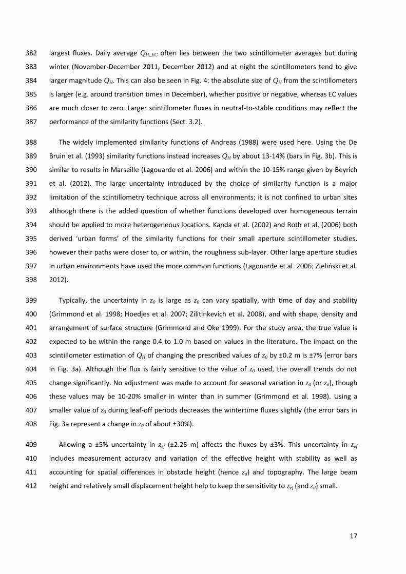
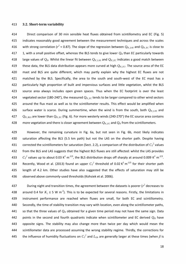
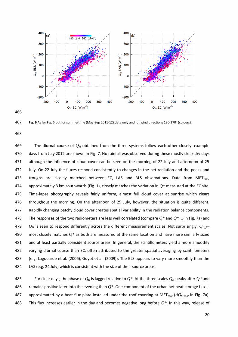
Direct comparison of 30 min sensible heat fluxes obtained from scintillometry and EC (Fig. 5) 414

indicates reasonably good agreement between the measurement techniques and across the scales 415

with strong correlation (r2 ≈ 0.87). The slope of the regression between QH_LAS and QH_EC is close to 416

1, with a small positive offset, whereas the BLS tends to give lower QH than EC particularly towards 417

large values of QH. Whilst the linear fit between QH_LAS and QH_EC indicates a good match between 418

these data, the BLS data distribution appears more curved at high QH_EC. The source area of the EC 419

mast and BLS are quite different, which may partly explain why the highest EC fluxes are not 420

matched by the BLS. Specifically, the area to the south and south-west of the EC mast has a 421

particularly high proportion of built and impervious surfaces and little vegetation, whilst the BLS 422

source area always includes open green spaces. Thus when the EC footprint is over the least 423

vegetated sector (180-240°), the measured QH_EC tends to be larger compared to other wind sectors 424

around the flux mast as well as to the scintillometer results. This effect would be amplified when 425

surface water is scarce. During summertime, when the wind is from the south, both QH_LAS and 426

QH_BLS are lower than QH_EC (Fig. 6). For more westerly winds (240-270°) the EC source area contains 427

more vegetation and there is closer agreement between QH_EC and QH from the scintillometers. 428

However, the remaining curvature in Fig. 6a, but not seen in Fig. 6b, most likely indicates 429

saturation affecting the BLS (5.5 km path) but not the LAS on the shorter path. Despite having 430

corrected the scintillometers for saturation (Sect. 2.2), a comparison of the distribution of CT2 values 431

from the BLS and LAS suggests that the highest BLS fluxes are still affected: whilst the LAS provides 432

CT2 values up to about 0.03 K2 m-2/3, the BLS distribution drops off sharply at around 0.009 K2 m-2/3. 433

Recently, Wood et al. (2013) found an upper CT2 threshold of 0.02 K2 m-2/3 for their shorter path 434

length of 4.2 km. Other studies have also suggested that the effects of saturation may still be 435

observed above commonly-used thresholds (Kohsiek et al. 2006). 436

During night and transition times, the agreement between the datasets is poorer (r2 decreases to 437

around 0.4 for K↓ ≤ 5 W m-2). This is to be expected for several reasons. Firstly, the limitations in 438

instrument performance are reached when fluxes are small, for both EC and scintillometry. 439

Secondly, the time of stability transition may vary with location, even along the scintillometer paths, 440

so that the three values of QH obtained for a given time period may not have the same sign. Data 441

points in the second and fourth quadrants indicate when scintillometer and EC derived QH have 442

opposite signs. The stability may also change more than twice per day which would mean the 443

scintillometer data are processed assuming the wrong stability regime. Thirdly, the corrections for 444

the influence of humidity fluctuations on CT2 and LOb are generally larger at these times (when β is 445

19

small). The Bowen ratio correction to CT2 introduces the larger error of these two approximations; 446

neglecting the buoyancy correction to the Obukhov length (e.g. Green et al. (2001)) is thought to 447

lead to a slight underestimation in QH of ≈ 0.5 W m-2. Finally, near-neutral to stable atmospheric 448

conditions do not always satisfy the assumptions required for the measurement theory (e.g. weak 449

turbulence, non-stationarity, poorer performance of similarity functions). Removing the night time 450

data causes the regression slopes in Fig. 5 to decrease slightly to 0.77 (BLS) and 0.94 (LAS), and the 451

intercepts to increase to 13 W m-2 (BLS) and 9 W m-2 (LAS). For night time data only, the intercepts 452

are similar in size but of opposite sign. These intercepts are thought to result from the 453

overestimation of small fluxes by the similarity functions. Considering all data together (Fig. 5) the 454

lack of small QH values from the scintillometers can be identified around zero. Using functions of a 455

conventional form (such as Equations 2 and 3) appears to under represent QH values close to zero 456

and overestimates QH in neutral conditions (fMO is too small so the T* obtained is too large). 457

Investigation into the scaling of CT2 with stability is presented in more detail elsewhere (Ward et al. 458

in preparation a) and Lagouarde et al. (2006) also noted an overestimation (15 W m-2) of small night 459

time QH values using An88 and DB93 (unstable forms). Although this effect is undesirable, the small 460

size of the fluxes at these times means that absolute errors are small. 461

462

463

Fig. 5 Comparison of 30 min sensible heat fluxes derived from the scintillometers (BLS, LAS) and eddy covariance (EC) for all 464

available data. 465

20

466

Fig. 6 As for Fig. 5 but for summertime (May-Sep 2011-12) data only and for wind directions 180-270° (colours). 467

468

The diurnal course of QH obtained from the three systems follow each other closely: example 469

days from July 2012 are shown in Fig. 7. No rainfall was observed during these mostly clear-sky days 470

although the influence of cloud cover can be seen on the morning of 22 July and afternoon of 25 471

July. On 22 July the fluxes respond consistently to changes in the net radiation and the peaks and 472

troughs are closely matched between EC, LAS and BLS observations. Data from METroof, 473

approximately 3 km southwards (Fig. 1), closely matches the variation in Q* measured at the EC site. 474

Time-lapse photography reveals fairly uniform, almost full cloud cover at sunrise which clears 475

throughout the morning. On the afternoon of 25 July, however, the situation is quite different. 476

Rapidly changing patchy cloud cover creates spatial variability in the radiation balance components. 477

The responses of the two radiometers are less well correlated (compare Q* and Q*roof in Fig. 7a) and 478

QH is seen to respond differently across the different measurement scales. Not surprisingly, QH_EC 479

most closely matches Q* as both are measured at the same location and have more similarly sized 480

and at least partially coincident source areas. In general, the scintillometers yield a more smoothly 481

varying diurnal course than EC, often attributed to the greater spatial averaging by scintillometers 482

(e.g. Lagouarde et al. (2006), Guyot et al. (2009)). The BLS appears to vary more smoothly than the 483

LAS (e.g. 24 July) which is consistent with the size of their source areas. 484

For clear days, the phase of QH is lagged relative to Q*. At the three scales QH peaks after Q* and 485

remains positive later into the evening than Q*. One component of the urban net heat storage flux is 486

approximated by a heat flux plate installed under the roof covering at METroof (ΔQS_roof in Fig. 7a). 487

This flux increases earlier in the day and becomes negative long before Q*. In this way, release of 488

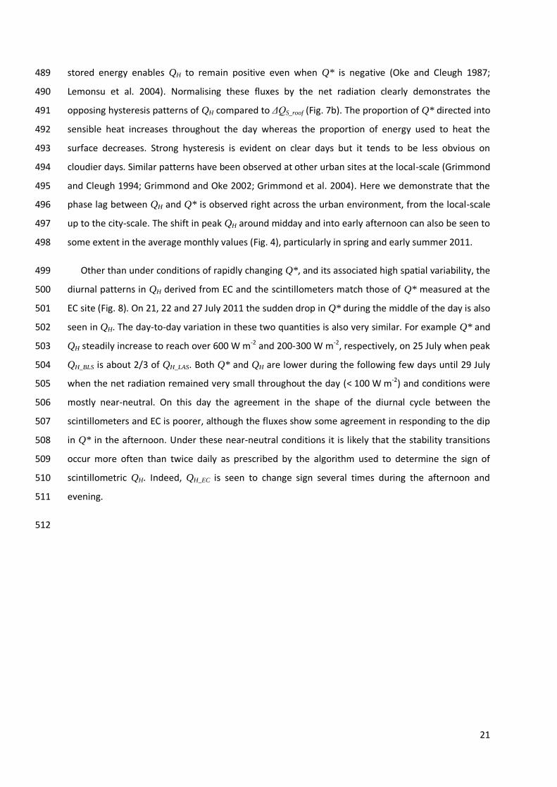
21

stored energy enables QH to remain positive even when Q* is negative (Oke and Cleugh 1987; 489

Lemonsu et al. 2004). Normalising these fluxes by the net radiation clearly demonstrates the 490

opposing hysteresis patterns of QH compared to ΔQS_roof (Fig. 7b). The proportion of Q* directed into 491

sensible heat increases throughout the day whereas the proportion of energy used to heat the 492

surface decreases. Strong hysteresis is evident on clear days but it tends to be less obvious on 493

cloudier days. Similar patterns have been observed at other urban sites at the local-scale (Grimmond 494

and Cleugh 1994; Grimmond and Oke 2002; Grimmond et al. 2004). Here we demonstrate that the 495

phase lag between QH and Q* is observed right across the urban environment, from the local-scale 496

up to the city-scale. The shift in peak QH around midday and into early afternoon can also be seen to 497

some extent in the average monthly values (Fig. 4), particularly in spring and early summer 2011. 498

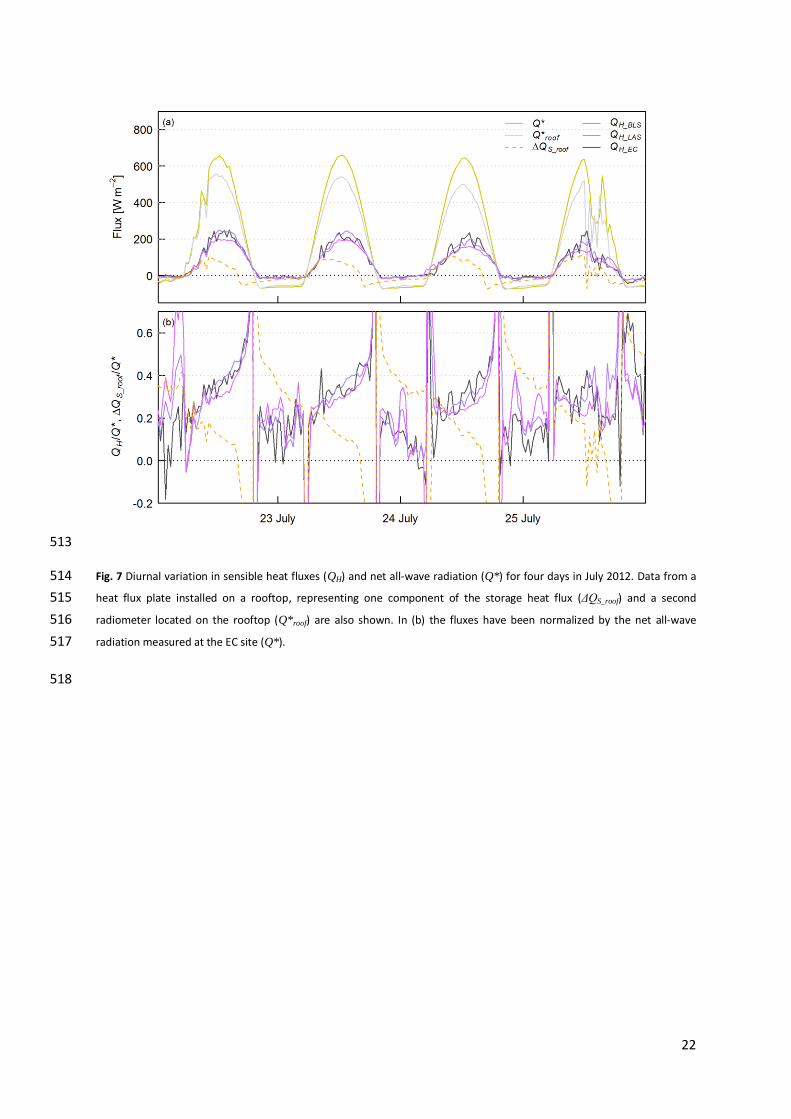
Other than under conditions of rapidly changing Q*, and its associated high spatial variability, the 499

diurnal patterns in QH derived from EC and the scintillometers match those of Q* measured at the 500

EC site (Fig. 8). On 21, 22 and 27 July 2011 the sudden drop in Q* during the middle of the day is also 501

seen in QH. The day-to-day variation in these two quantities is also very similar. For example Q* and 502

QH steadily increase to reach over 600 W m-2 and 200-300 W m-2, respectively, on 25 July when peak 503

QH_BLS is about 2/3 of QH_LAS. Both Q* and QH are lower during the following few days until 29 July 504

when the net radiation remained very small throughout the day (< 100 W m-2) and conditions were 505

mostly near-neutral. On this day the agreement in the shape of the diurnal cycle between the 506

scintillometers and EC is poorer, although the fluxes show some agreement in responding to the dip 507

in Q* in the afternoon. Under these near-neutral conditions it is likely that the stability transitions 508

occur more often than twice daily as prescribed by the algorithm used to determine the sign of 509

scintillometric QH. Indeed, QH_EC is seen to change sign several times during the afternoon and 510

evening. 511

512

22

513

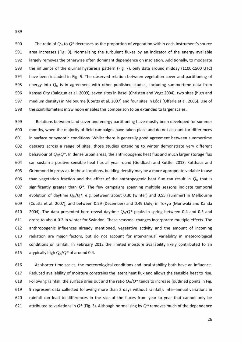
Fig. 7 Diurnal variation in sensible heat fluxes (QH) and net all-wave radiation (Q*) for four days in July 2012. Data from a 514

heat flux plate installed on a rooftop, representing one component of the storage heat flux (ΔQS_roof) and a second 515

radiometer located on the rooftop (Q*roof) are also shown. In (b) the fluxes have been normalized by the net all-wave 516

radiation measured at the EC site (Q*). 517

518

23

519

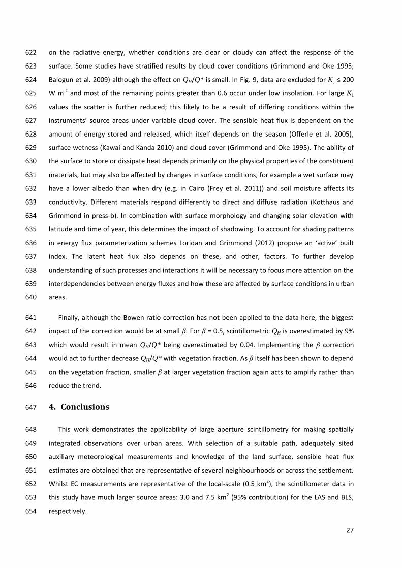
Fig. 8 Sensible heat fluxes from EC and the scintillometers alongside net all-wave radiation from the EC site (Q*), rainfall 520

and wind direction (also measured at the EC site) for two weeks in July-August 2011. 521

522

The sign of the scintillometer sensible heat flux must be assigned during processing. Here, the 523

stability was assumed to change from stable to unstable at the first minimum in Cn2 on each day, and 524

from unstable to stable at the second minimum, providing these transitions occurred within the 525

likely time frames for sunrise and sunset. Additionally, the net radiation can be used to check 526

whether the minima identified are likely to indicate stability transitions rather than sudden increases 527

in cloud cover, for example. For each 24 h period the algorithm always results in some stable and 528

some unstable data and the proportion of each depends on the observed behaviour of Cn2 529

(effectively on the time between the morning and evening minima). As is evident from the data, this 530

method generally performs well in Swindon, where EC data suggests QH tends to be positive for 531

some duration around midday and negative at night (Ward et al. 2013a). However, there are some 532

days when the stability transition does not occur and either unstable conditions prevail throughout 533

the night or stable conditions throughout the day. In these cases the sign of the fluxes from the 534

24

scintillometers may be incorrect but these occasions are observed infrequently and the size of the 535

fluxes tends to be small so the likely impact is minimal. 536

The day-to-day (night-to-night) changes in amplitude are usually captured (e.g. decreasing 537

magnitude of nocturnal QH 24-27 July 2011 in Fig. 8b) and for some days the evolution of QH 538

throughout the night is similar (e.g. decreasing 20-21, increasing 25-26 and 26-27 July 2011, Fig. 8b). 539

This clear relation between the scintillometer and EC fluxes gives confidence that the measurement 540

heights are suitable; in particular that the scintillometers are not measuring above the surface layer. 541

In the winter months, occasionally there are periods of a few hours to days when the shallow surface 542

layer means the scintillometer measurements cannot be related to surface fluxes via MOST (Braam 543

et al. 2012). The EC data further supports these findings with very few cases of strongly stable 544

stratification observed (ζEC < 0.1 for 89% of data). 545

3.3. Influence of the surface 546

Comparing the relative sizes of the fluxes can offer insight into key controls on suburban energy 547

partitioning. Towards the end of the case study in Fig. 8 (30 July-01 August 2011), QH_EC peaks at 548

larger values than either of the scintillometers, whilst QH_LAS is generally largest near the beginning 549

of the period (21-25 July). The wind direction (Fig. 8c) provides a partial explanation due to the 550

variation in source areas. For westerly to northerly winds, QH_LAS tends to be largest. All three fluxes 551

become similar during northerly winds, when there is a greater vegetation fraction within the source 552

area of each instrument. For the scintillometers the footprint will extend to include some of the rural 553

farmland beyond the edge of the suburbs; at the EC site the increased vegetation is due to more 554

gardens to the north of the mast (Ward et al. 2013a). 555

The period shown in Fig. 9 (21 May – 31 July 2012) coincides with sudden vegetation growth in 556

response to warm, sunny conditions at the end of May, completing the leaf-out period to reach 557

maturity. Vegetation is then fully active throughout June and July. In this period a range of synoptic 558

conditions (cloudy, mixed and clear days), frequent rainfall and a wide distribution of wind directions 559

(although south-westerly was still dominant) occurred. 560

Footprint calculations for each 30 min period reveal an overall ranking of the vegetation fraction 561

for each instrument that is in accordance with broad expectations given their respective sitings (EC < 562

LAS < BLS). The mean vegetation fractions (± standard deviations) are 44.1 (±5.0) %, 53.9 (±2.9) % 563

and 56.9 (±4.5) % for EC, LAS and BLS, respectively, for the data shown in Fig. 9. The standard 564

deviation is largest for the EC site, as might be expected (a) given the far smaller size of the source 565

area and (b) the differences in surface cover with wind sector around the mast. The vegetation 566

25

fraction ranges between 32.6% and 56.8% according to the EC footprint estimation for this period. 567

The LAS source area characteristics are much less variable (minimum 47.7%, maximum 60.2%). The 568

retail park to the west of the path (Fig. 1) constitutes a small proportion of the total source area and 569

for westerly wind directions there is only a small increase in the built and impervious fractions. 570

Despite having the largest area, the BLS footprint shows appreciable variability (48.3% – 65.7%), 571

mostly associated with southerly or northerly winds when the town centre and nearby industrial 572

areas (Fig. 1) or rural surroundings are included in the footprint. For small changes in wind direction 573

the BLS source area composition hardly changes, whereas the EC source area composition can vary 574

considerably (particularly for the 180-270° sector). In addition to the directional aspect of the 575

surface heterogeneity, the total area included in the scintillometer footprint is smaller when the 576

wind direction is parallel, as opposed to perpendicular, to the scintillometer path (Meijninger et al. 577

2002b). In this case, the spatial integration occurs over a smaller area so the footprint composition, 578

and observed fluxes, may be expected to be more variable. 579

580

581

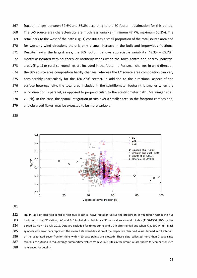
Fig. 9 Ratio of observed sensible heat flux to net all-wave radiation versus the proportion of vegetation within the flux 582

footprint of the EC station, LAS and BLS in Swindon. Points are 30 min values around midday (1100-1500 UTC) for the 583

period 21 May – 31 July 2012. Data are excluded for times during and ≤ 2 h after rainfall and when K↓ ≤ 200 W m-2. Black 584

symbols with error bars represent the mean ± standard deviation of the respective observed values binned in 5% intervals 585

of the vegetated cover fraction (bins with > 10 data points are plotted). Those data collected more than 2 days since 586

rainfall are outlined in red. Average summertime values from various sites in the literature are shown for comparison (see 587

references for details). 588

26

589

The ratio of QH to Q* decreases as the proportion of vegetation within each instrument’s source 590

area increases (Fig. 9). Normalising the turbulent fluxes by an indicator of the energy available 591

largely removes the otherwise often dominant dependence on insolation. Additionally, to moderate 592

the influence of the diurnal hysteresis pattern (Fig. 7), only data around midday (1100-1500 UTC) 593

have been included in Fig. 9. The observed relation between vegetation cover and partitioning of 594

energy into QH is in agreement with other published studies, including summertime data from 595

Kansas City (Balogun et al. 2009), seven sites in Basel (Christen and Vogt 2004), two sites (high and 596

medium density) in Melbourne (Coutts et al. 2007) and four sites in Łódź (Offerle et al. 2006). Use of 597

the scintillometers in Swindon enables this comparison to be extended to larger scales. 598

Relations between land cover and energy partitioning have mostly been developed for summer 599

months, when the majority of field campaigns have taken place and do not account for differences 600

in surface or synoptic conditions. Whilst there is generally good agreement between summertime 601

datasets across a range of sites, those studies extending to winter demonstrate very different 602

behaviour of QH/Q*. In dense urban areas, the anthropogenic heat flux and much larger storage flux 603

can sustain a positive sensible heat flux all year round (Goldbach and Kuttler 2013; Kotthaus and 604

Grimmond in press-a). In these locations, building density may be a more appropriate variable to use 605

than vegetation fraction and the effect of the anthropogenic heat flux can result in QH that is 606

significantly greater than Q*. The few campaigns spanning multiple seasons indicate temporal 607

evolution of daytime QH/Q*, e.g. between about 0.30 (winter) and 0.55 (summer) in Melbourne 608

(Coutts et al. 2007), and between 0.29 (December) and 0.49 (July) in Tokyo (Moriwaki and Kanda 609

2004). The data presented here reveal daytime QH/Q* peaks in spring between 0.4 and 0.5 and 610

drops to about 0.2 in winter for Swindon. These seasonal changes incorporate multiple effects. The 611

anthropogenic influences already mentioned, vegetative activity and the amount of incoming 612

radiation are major factors, but do not account for inter-annual variability in meteorological 613

conditions or rainfall. In February 2012 the limited moisture availability likely contributed to an 614

atypically high QH/Q* of around 0.4. 615

At shorter time scales, the meteorological conditions and local stability both have an influence. 616

Reduced availability of moisture constrains the latent heat flux and allows the sensible heat to rise. 617

Following rainfall, the surface dries out and the ratio QH/Q* tends to increase (outlined points in Fig. 618

9 represent data collected following more than 2 days without rainfall). Inter-annual variations in 619

rainfall can lead to differences in the size of the fluxes from year to year that cannot only be 620

attributed to variations in Q* (Fig. 3). Although normalising by Q* removes much of the dependence 621

27

on the radiative energy, whether conditions are clear or cloudy can affect the response of the 622

surface. Some studies have stratified results by cloud cover conditions (Grimmond and Oke 1995; 623

Balogun et al. 2009) although the effect on QH/Q* is small. In Fig. 9, data are excluded for K↓ ≤ 200 624

W m-2 and most of the remaining points greater than 0.6 occur under low insolation. For large K↓ 625

values the scatter is further reduced; this likely to be a result of differing conditions within the 626

instruments’ source areas under variable cloud cover. The sensible heat flux is dependent on the 627

amount of energy stored and released, which itself depends on the season (Offerle et al. 2005), 628

surface wetness (Kawai and Kanda 2010) and cloud cover (Grimmond and Oke 1995). The ability of 629

the surface to store or dissipate heat depends primarily on the physical properties of the constituent 630

materials, but may also be affected by changes in surface conditions, for example a wet surface may 631

have a lower albedo than when dry (e.g. in Cairo (Frey et al. 2011)) and soil moisture affects its 632

conductivity. Different materials respond differently to direct and diffuse radiation (Kotthaus and 633

Grimmond in press-b). In combination with surface morphology and changing solar elevation with 634

latitude and time of year, this determines the impact of shadowing. To account for shading patterns 635

in energy flux parameterization schemes Loridan and Grimmond (2012) propose an ‘active’ built 636

index. The latent heat flux also depends on these, and other, factors. To further develop 637

understanding of such processes and interactions it will be necessary to focus more attention on the 638

interdependencies between energy fluxes and how these are affected by surface conditions in urban 639

areas. 640

Finally, although the Bowen ratio correction has not been applied to the data here, the biggest 641

impact of the correction would be at small β. For β = 0.5, scintillometric QH is overestimated by 9% 642

which would result in mean QH/Q* being overestimated by 0.04. Implementing the β correction 643

would act to further decrease QH/Q* with vegetation fraction. As β itself has been shown to depend 644

on the vegetation fraction, smaller β at larger vegetation fraction again acts to amplify rather than 645

reduce the trend. 646

4. Conclusions 647

This work demonstrates the applicability of large aperture scintillometry for making spatially 648

integrated observations over urban areas. With selection of a suitable path, adequately sited 649

auxiliary meteorological measurements and knowledge of the land surface, sensible heat flux 650

estimates are obtained that are representative of several neighbourhoods or across the settlement. 651

Whilst EC measurements are representative of the local-scale (0.5 km2), the scintillometer data in 652

this study have much larger source areas: 3.0 and 7.5 km2 (95% contribution) for the LAS and BLS, 653

respectively. 654

28

Remarkable temporal agreement is observed across the three different areal extents for both 655

short-term variability (e.g. the response to radiation patterns over a few hours to days) and seasonal 656

trends. Differences in magnitudes of the fluxes between sites are attributed primarily to the role of 657

vegetation and reveal the influence of anthropogenic materials on surface-atmosphere interactions. 658

Empirical relations between land cover and fluxes often underpin urban energy models and are 659

valuable for gauging the likely partitioning of energy, and hence the environmental conditions 660

(including thermal comfort and moisture availability), in cities where measurements have not been 661

made. 662

Comparison of the EC dataset with large-area fluxes at the city-scale provides some context to 663

the results and confirms that the EC site selection was appropriate. The scintillometer fluxes tend to 664

be smoother as a result of the greater spatial averaging. The large-scale flux measurements are also 665

much less sensitive to source area variability, for example due to changing wind direction over 666

heterogeneous surfaces. As they encompass a larger proportion of the study area, these large-area 667

fluxes are more representative and suffer less from sampling bias, whereas EC measurements are 668

easily influenced by spatially variable land cover or surface characteristics around the mast. The 669

effect can be decreased by measuring at a greater height, but in general the land cover must be 670

carefully examined for each wind sector before drawing conclusions on the representativeness of 671

data from a single EC site. 672

For many purposes we are interested in fluxes at large scales, whether the application is input 673

data for, or evaluation of, land-surface models or numerical weather prediction, assessment of 674

satellite remote sensing products or representative observational datasets to characterize a 675

particular environment. Scintillometry offers a promising way forward, but there are still limitations. 676

A major source of uncertainty arises from the MOST functions. This is an area that would benefit 677

from further attention for all land cover types and has implications beyond improving the accuracy 678

of fluxes from scintillometry. Single-wavelength scintillometry may be best suited to urban areas 679

with little vegetation as the higher the Bowen ratio the smaller the error due to neglecting the β-680

correction (Moene 2003). Given the potential for saturation, particularly if the sensible heat flux is 681

large, it is recommended that an extra-large aperture scintillometer is considered for long paths (e.g. 682

> 4 km, for paths of similar height and fluxes of similar magnitude). Future work will likely focus on 683

the development of the scintillometry technique and the application for routine monitoring at large-684

scales, e.g. Kleissl et al. (2009a). Such observational networks would offer valuable data for 685

assimilation into models that assess e.g. air quality or heat stress, both highly relevant to human 686

health and well-being. 687

29

Acknowledgements 688

We gratefully acknowledge the support of the following CEH staff: Alan Warwick and Cyril Barrett 689

for design and construction of the scintillometer mountings, Geoff Wicks for assistance with the 690

electronics and Dave McNeil for helping to build the rooftop weather station. This work would not 691

have been possible without the generous co-operation of several people in Swindon who very kindly 692

gave permission for equipment to be installed on their property. We also wish to thank the Science 693

and Technology Facilities Council staff at Chilbolton Observatory for use of their test range for the 694

scintillometer comparison. This work was funded by the Natural Environment Research Council, UK. 695

696

References 697

Andreas EL (1988) Estimating Cn2 over snow and sea ice from meteorological data. J Opt Soc Am 5: 698

481-495. 699 Andreas EL (1989) Two-wavelength method of measuring path-averaged turbulent surface heat 700

fluxes. J Atmos Ocean Technol 6: 280-292. 701 Balogun A, Adegoke J, Vezhapparambu S, Mauder M, McFadden J and Gallo K (2009) Surface energy 702

balance measurements above an exurban residential neighbourhood of Kansas City, 703 Missouri. Boundary-Layer Meteorol 133: 299-321. doi: 10.1007/s10546-009-9421-3 704

Bergeron O and Strachan IB (2010) Wintertime radiation and energy budget along an urbanization 705 gradient in Montreal, Canada. Int J Climatol 32: 137-152. doi: 10.1002/joc.2246 706

Beyrich F, Bange J, Hartogensis O, Raasch S, Braam M, van Dinther D, Gräf D, van Kesteren B, van 707 den Kroonenberg A, Maronga B, Martin S and Moene A (2012) Towards a Validation of 708 Scintillometer Measurements: The LITFASS-2009 Experiment. Boundary-Layer Meteorol 144: 709 83-112. doi: 10.1007/s10546-012-9715-8 710

Beyrich F, De Bruin HAR, Meijninger WML, Schipper JW and Lohse H (2002) Results from one-year 711 continuous operation of a large aperture scintillometer over a heterogeneous land surface. 712 Boundary-Layer Meteorol 105: 85-97. 713

Braam M, Bosveld F and Moene A (2012) On Monin–Obukhov Scaling in and Above the Atmospheric 714 Surface Layer: The Complexities of Elevated Scintillometer Measurements. Boundary-Layer 715 Meteorol 144: 157-177. doi: 10.1007/s10546-012-9716-7 716

Chehbouni A, Watts C, Kerr YH, Dedieu G, Rodriguez JC, Santiago F, Cayrol P, Boulet G and Goodrich 717 DC (2000a) Methods to aggregate turbulent fluxes over heterogeneous surfaces: application 718 to SALSA data set in Mexico. Agric For Meteorol 105: 133-144. 719

Chehbouni A, Watts C, Lagouarde JP, Kerr YH, Rodriguez JC, Bonnefond JM, Santiago F, Dedieu G, 720 Goodrich DC and Unkrich C (2000b) Estimation of heat and momentum fluxes over complex 721 terrain using a large aperture scintillometer. Agric For Meteorol 105: 215-226. 722

Cheinet S, Beljaars A, Weiss-Wrana K and Hurtaud Y (2011) The Use of Weather Forecasts to 723 Characterise Near-Surface Optical Turbulence. Boundary-Layer Meteorol 138: 453-473. doi: 724 10.1007/s10546-010-9567-z 725

Christen A and Vogt R (2004) Energy and radiation balance of a central European city. Int J Climatol 726 24: 1395-1421. doi: 10.1002/joc.1074 727

Clifford SF, Ochs GR and Lawrence RS (1974) Saturation of optical scintillation by strong turbulence. J 728 Opt Soc Am 64: 148-154. 729

30

Coutts AM, Beringer J and Tapper NJ (2007) Impact of increasing urban density on local climate: 730 Spatial and temporal variations in the surface energy balance in Melbourne, Australia. J Appl 731 Meteorol Climatol 46: 477-493. doi: 10.1175/jam2462.1 732

De Bruin HAR, Kohsiek W and Van den Hurk BJJM (1993) A verification of some methods to 733 determine the fluxes of momentum, sensible heat, and water-vapour using standard-734 deviation and structure parameter of scalar meteorological quantities. Boundary-Layer 735 Meteorol 63: 231-257. 736

Detto M, Montaldo N, Albertson JD, Mancini M and Katul G (2006) Soil moisture and vegetation 737 controls on evapotranspiration in a heterogeneous Mediterranean ecosystem on Sardinia, 738 Italy. Water Resour Res 42: 16. doi: 10.1029/2005wr004693 739

Evans JG (2009) Long-Path Scintillometry over Complex Terrain to Determine Areal-Averaged 740 Sensible and Latent Heat Fluxes. Soil Science Department, The University of Reading, PhD, 741 181 pp 742

Evans JG, McNeil DD, Finch JW, Murray T, Harding RJ, Ward HC and Verhoef A (2012) Determination 743 of turbulent heat fluxes using a large aperture scintillometer over undulating mixed 744 agricultural terrain. Agric For Meteorol 166-167: 221-233. 745

Ezzahar J, Chehbouni A and Hoedjes JCB (2007) On the application of scintillometry over 746 heterogeneous grids. J Hydrol 334: 493-501. doi: 10.1016/j.jhydrol.2006.10.027 747

Frey CM, Parlow E, Vogt R, Harhash M and Abdel Wahab MM (2011) Flux measurements in Cairo. 748 Part 1: in situ measurements and their applicability for comparison with satellite data. Int J 749 Climatol 31: 218-231. doi: 10.1002/joc.2140 750

Garratt JR (1978) Transfer characteristics for a heterogeneous surface of large aerodynamic 751 roughness. Q J R Meteorol Soc 104: 491-502. doi: 10.1002/qj.49710444019 752

Garratt JR (1992) The Atmospheric Boundary Layer, Cambridge University Press, 316 pp 753 Goldbach A and Kuttler W (2013) Quantification of turbulent heat fluxes for adaptation strategies 754

within urban planning. Int J Climatol 33: 143-159. doi: 10.1002/joc.3437 755 Gouvea ML and Grimmond CSB (2010) Spatially integrated measurements of sensible heat flux using 756

scintillometry. Ninth Symposium on the Urban Environment, Keystone, Colorado, 2nd-6th 757 August 2010 758

Green AE, Astill MS, McAneney KJ and Nieveen JP (2001) Path-averaged surface fluxes determined 759 from infrared and microwave scintillometers. Agric For Meteorol 109: 233-247. 760

Grimmond CSB and Cleugh HA (1994) A Simple Method to Determine Obukhov Lengths for Suburban 761 Areas. J Appl Meteorol 33: 435-440. 762

Grimmond CSB, King TS, Roth M and Oke TR (1998) Aerodynamic roughness of urban areas derived 763 from wind observations. Boundary-Layer Meteorol 89: 1-24. 764

Grimmond CSB and Oke TR (1995) Comparison of Heat Fluxes from Summertime Observations in the 765 Suburbs of Four North American Cities. J Appl Meteorol 34: 873-889. doi: 10.1175/1520-766 0450 767

Grimmond CSB and Oke TR (1999) Aerodynamic properties of urban areas derived from analysis of 768 surface form. J Appl Meteorol 38: 1262-1292. 769

Grimmond CSB and Oke TR (2002) Turbulent heat fluxes in urban areas: Observations and a local-770 scale urban meteorological parameterization scheme (LUMPS). J Appl Meteorol 41: 792-810. 771

Grimmond CSB, Salmond JA, Oke TR, Offerle B and Lemonsu A (2004) Flux and turbulence 772 measurements at a densely built-up site in Marseille: Heat, mass (water and carbon dioxide), 773 and momentum. J Geophys Res (Atmos) 109: D24101. doi: D2410110.1029/2004jd004936 774

Grimmond CSB, Souch C and Hubble MD (1996) Influence of tree cover on summertime surface 775 energy balance fluxes, San Gabriel Valley, Los Angeles. Climate Res 06: 45-57. doi: 776 10.3354/cr006045 777

Guyot A, Cohard J-M, Anquetin S, Galle S and Lloyd CR (2009) Combined analysis of energy and 778 water balances to estimate latent heat flux of a Sudanian small catchment. J Hydrol 375: 779 227-240. 780

31

Hartogensis OK, Watts CJ, Rodriguez JC and De Bruin HAR (2003) Derivation of an effective height for 781 scintillometers: La Poza experiment in Northwest Mexico. J Hydrometerol 4: 915-928. 782

Hill RJ, Bohlander RA, Clifford SF, McMillan RW, Priestly JT and Schoenfeld WP (1988) Turbulence-783 induced millimeter-wave scintillation compared with micrometeorological measurements. 784 IEEE Trans Geosci Remote Sens 26: 330-342. 785

Hill RJ, Clifford SF and Lawrence RS (1980) Refractive-index and absorption fluctuations in the 786 infrared caused by temperature, humidity, and pressure fluctuations. J Opt Soc Am 70: 1192-787 1205. 788

Hill RJ, Ochs GR and Wilson JJ (1992) Measuring surface-layer fluxes of heat and momentum using 789 optical scintillation. Boundary-Layer Meteorol 58: 391-408. doi: 10.1007/bf00120239 790

Hiller RV, McFadden JP and Kljun N (2011) Interpreting CO2 Fluxes Over a Suburban Lawn: The 791 Influence of Traffic Emissions. Boundary-Layer Meteorol 138: 215-230. doi: 10.1007/s10546-792 010-9558-0 793

Hoedjes JCB, Chehbouni A, Ezzahar J, Escadafal R and De Bruin HAR (2007) Comparison of large 794 aperture scintillometer and eddy covariance measurements: Can thermal infrared data be 795 used to capture footprint-induced differences? J Hydrometerol 8: 144-159. doi: 796 10.1175/jhm561.1 797

Hoedjes JCB, Zuurbier RM and Watts CJ (2002) Large aperture scintillometer used over a 798 homogeneous irrigated area, partly affected by regional advection. Boundary-Layer 799 Meteorol 105: 99-117. 800

Hsieh CI, Katul G and Chi T (2000) An approximate analytical model for footprint estimation of scalar 801 fluxes in thermally stratified atmospheric flows. Adv Water Resour 23: 765-772. 802

Järvi L, Grimmond CSB and Christen A (2011) The Surface Urban Energy and Water Balance Scheme 803 (SUEWS): Evaluation in Los Angeles and Vancouver. J Hydrol 411: 219-237. 804

Järvi L, Nordbo A, Junninen H, Riikonen A, Moilanen J, Nikinmaa E and Vesala T (2012) Seasonal and 805 annual variation of carbon dioxide surface fluxes in Helsinki, Finland, in 2006-2010. Atmos 806 Chem Phys 12: 8475-8489. doi: 10.5194/acp-12-8475-2012 807

Järvi L, Rannik U, Mammarella I, Sogachev A, Aalto PP, Keronen P, Siivola E, Kulmala M and Vesala T 808 (2009) Annual particle flux observations over a heterogeneous urban area. Atmos Chem 809 Phys 9: 7847-7856. 810

Kanda M, Moriwaki R, Roth M and Oke T (2002) Area-averaged sensible heat flux and a new method 811 to determine zero-plane displacement length over an urban surface using scintillometry. 812 Boundary-Layer Meteorol 105: 177-193. 813

Kawai T and Kanda M (2010) Urban Energy Balance Obtained from the Comprehensive Outdoor 814 Scale Model Experiment. Part I: Basic Features of the Surface Energy Balance. J Appl 815 Meteorol Climatol 49: 1341-1359. doi: 10.1175/2010jamc1992.1 816

Keogh S, Mills G and Fealy R (2012) The energy budget of the urban surface: two locations in Dublin. 817 Irish Geography 45: 1-23. doi: 10.1080/00750778.2012.689182 818

Kleissl J, Gomez J, Hong SH, Hendrickx JMH, Rahn T and Defoor WL (2008) Large aperture 819 scintillometer intercomparison study. Boundary-Layer Meteorol 128: 133-150. doi: 820 10.1007/s10546-008-9274-1 821

Kleissl J, Hartogensis O and Gomez J (2010) Test of Scintillometer Saturation Correction Methods 822 Using Field Experimental Data. Boundary-Layer Meteorol 137: 493-507. doi: 823 10.1007/s10546-010-9540-x 824

Kleissl J, Hong SH and Hendrickx JMH (2009a) New Mexico scintillometer network supporting remote 825 sensing and hydrologic and meteorological models. Bull Am Meteorol Soc 90: 207-218. doi: 826 10.1175/2008bams2480.1 827

Kleissl J, Watts CJ, Rodriguez JC, Naif S and Vivoni ER (2009b) Scintillometer Intercomparison Study-828 Continued. Boundary-Layer Meteorol 130: 437-443. doi: 10.1007/s10546-009-9352-z 829

Kohsiek W and Herben MHAJ (1983) Evaporation derived from optical and radio-wave scintillation. 830 Appl Opt 22: 2566-2570. 831

32

Kohsiek W, Meijninger WML, De Bruin HAR and Beyrich F (2006) Saturation of the Large Aperture 832 Scintillometer. Boundary-Layer Meteorol 121: 111-126. doi: 10.1007/s10546-005-9031-7 833

Kotthaus S and Grimmond CSB (in press-a) Energy exchange in a dense urban environment - Part I: 834 temporal variability of long-term observations in central London. Urban Climate. doi: 835 10.1016/j.uclim.2013.10.002 836

Kotthaus S and Grimmond CSB (in press-b) Energy exchange in a dense urban environment – Part II: 837 impact of spatial heterogeneity of the surface. Urban Climate. doi: 838 10.1016/j.uclim.2013.10.001 839

Lagouarde JP, Irvine M, Bonnefond JM, Grimmond CSB, Long N, Oke TR, Salmond JA and Offerle B 840 (2006) Monitoring the sensible heat flux over urban areas using large aperture 841 scintillometry: Case study of Marseille city during the ESCOMPTE experiment. Boundary-842 Layer Meteorol 118: 449-476. doi: 10.1007/s10546-005-9001-0 843

Lemonsu A, Grimmond CSB and Masson V (2004) Modeling the surface energy balance of the core of 844 an old Mediterranean city: Marseille. J Appl Meteorol 43: 312-327. 845

Liu SM, Xu ZW, Zhu ZL, Jia ZZ and Zhu MJ (2013) Measurements of evapotranspiration from eddy-846 covariance systems and large aperture scintillometers in the Hai River Basin, China. J Hydrol 847 487: 24-38. doi: http://dx.doi.org/10.1016/j.jhydrol.2013.02.025 848

Loridan T and Grimmond CSB (2012) Characterization of Energy Flux Partitioning in Urban 849 Environments: Links with Surface Seasonal Properties. J Appl Meteorol Climatol 51: 219-241. 850 doi: 10.1175/jamc-d-11-038.1 851

Maronga B, Moene AF, Dinther D, Raasch S, Bosveld FC and Gioli B (2013) Derivation of Structure 852 Parameters of Temperature and Humidity in the Convective Boundary Layer from Large-853 Eddy Simulations and Implications for the Interpretation of Scintillometer Observations. 854 Boundary-Layer Meteorol 148: 1-30. doi: 10.1007/s10546-013-9801-6 855

Maronga B and Raasch S (2013) Large-Eddy Simulations of Surface Heterogeneity Effects on the 856 Convective Boundary Layer During the LITFASS-2003 Experiment. Boundary-Layer Meteorol 857 146: 17-44. doi: 10.1007/s10546-012-9748-z 858

Meijninger WML, Beyrich F, Lüdi A, Kohsiek W and De Bruin HAR (2006) Scintillometer-based 859 turbulent fluxes of sensible and latent heat over a heterogeneous land surface - A 860 contribution to LITFASS-2003. Boundary-Layer Meteorol 121: 89-110. doi: 10.1007/s10546-861 005-9022-8 862

Meijninger WML and De Bruin HAR (2000) The sensible heat fluxes over irrigated areas in western 863 Turkey determined with a large aperture scintillometer. J Hydrol 229: 42-49. 864

Meijninger WML, Green AE, Hartogensis OK, Kohsiek W, Hoedjes JCB, Zuurbier RM and De Bruin HAR 865 (2002a) Determination of area-averaged water vapour fluxes with large aperture and radio 866 wave scintillometers over a heterogeneous surface - Flevoland field experiment. Boundary-867 Layer Meteorol 105: 63-83. 868

Meijninger WML, Hartogensis OK, Kohsiek W, Hoedjes JCB, Zuurbier RM and De Bruin HAR (2002b) 869 Determination of area-averaged sensible heat fluxes with a large aperture scintillometer 870 over a heterogeneous surface - Flevoland field experiment. Boundary-Layer Meteorol 105: 871 37-62. 872

Mestayer P, Bagga I, Calmet I, Fontanilles G, Gaudin D, Lee JH, Piquet T, Rosant J-M, Chancibault K, 873 Lebouc L, Letellier L, Mosini M-L, Rodriguez F, Rouaud J-M, Sabre M, Tétard Y, Brut A, Selves 874 J-L, Solignac P-A, Brunet Y, Dayau S, Irvine M, Lagouarde J-P, Kassouk Z, Launeau P, Connan 875 O, Defenouillère P, Goriaux M, Hébert D, Letellier B, Mario D, Najjar G, Nerry F, Quentin C, 876 Biron R, Cohard J-M, Galvez J and Klein P (2011) The FluxSAP 2010 hydroclimatological 877 experimental campaign over an heterogeneous urban area. 11th EMS Annual Meeting, 878 Berlin, Germany, 12th-16th September 2011 879

Moene AF (2003) Effects of water vapour on the structure parameter of the refractive index for 880 near-infrared radiation. Boundary-Layer Meteorol 107: 635-653. 881

33

Moriwaki R and Kanda M (2004) Seasonal and diurnal fluxes of radiation, heat, water vapor, and 882 carbon dioxide over a suburban area. J Appl Meteorol 43: 1700-1710. 883

Mustchin J, Pauscher L, Ward HC, Kotthaus S, Gouvea M, Morrison W and Grimmond CSB (2013) 884 Comparison of Three Large Aperture Scintillometer Models Over London. Tübingen 885 Atmospheric Physics Symposium "Scintillometers and Applications", Tübingen, Germany, 886 7th-9th October 2013 887

Nordbo A, Järvi L, Haapanala S, Moilanen J and Vesala T (2013) Intra-City Variation in Urban 888 Morphology and Turbulence Structure in Helsinki, Finland. Boundary-Layer Meteorol 146: 889 469-496. doi: 10.1007/s10546-012-9773-y 890

Offerle B, Grimmond CSB and Fortuniak K (2005) Heat storage and anthropogenic heat flux in 891 relation to the energy balance of a central European city centre. Int J Climatol 25: 1405-892 1419. doi: 10.1002/koc.1198 893

Offerle B, Grimmond CSB, Fortuniak K and Pawlak W (2006) Intraurban differences of surface energy 894 fluxes in a central European city. J Appl Meteorol Climatol 45: 125-136. 895

Oke TR and Cleugh HA (1987) Urban heat storage derived as energy balance residuals. Boundary-896 Layer Meteorol 39: 233-245. doi: 10.1007/bf00116120 897

Pasquill F (1974) Atmospheric Diffusion, Wiley, 429 pp 898 Pauscher L (2010) Scintillometer Measurements above the Urban Area of London. Department of 899

Micrometeorology, University of Bayreuth, Diploma, 104 pp 900 Roberts SM, Oke TR, Grimmond CSB and Voogt JA (2006) Comparison of Four Methods to Estimate 901

Urban Heat Storage. J Appl Meteorol Climatol 45: 1766-1781. doi: 10.1175/jam2432.1 902 Roth M, Salmond JA and Satyanarayana ANV (2006) Methodological considerations regarding the 903

measurement of turbulent fluxes in the urban roughness sublayer: The role of 904 scintillometery. Boundary-Layer Meteorol 121: 351-375. doi: 10.1007/s10546-006-9074-4 905

Samain B, Defloor W and Pauwels VRN (2012) Continuous Time Series of Catchment-Averaged 906 Sensible Heat Flux from a Large Aperture Scintillometer: Efficient Estimation of Stability 907 Conditions and Importance of Fluxes under Stable Conditions. J Hydrometerol 13: 423-442. 908 doi: 10.1175/jhm-d-11-030.1 909

Samain B, Ferket BVA, Defloor W and Pauwels VRN (2011a) Estimation of catchment averaged 910 sensible heat fluxes using a large aperture scintillometer. Water Resour Res 47: W05536. 911 doi: 10.1029/2009wr009032 912

Samain B, Simons GWH, Voogt MP, Defloor W, Bink N-J and Pauwels VRN (2011b) Consistency 913 between hydrological model, large aperture scintillometer and remote sensing based 914 evapotranspiration estimates for a heterogeneous catchment. Hydrol Earth Syst Sci 8: 915 10863-10894. doi: 10.5194/hessd-8-10863-2011 916

Schmid HP (1994) Source areas for scalars and scalar fluxes. Boundary-Layer Meteorol 67: 293-318. 917 doi: 10.1007/bf00713146 918

Schmid HP, Cleugh HA, Grimmond CSB and Oke TR (1991) Spatial variability of energy fluxes in 919 suburban terrain. Boundary-Layer Meteorol 54: 249-276. doi: 10.1007/bf00183956 920

Steeneveld GJ, Tolk LF, Moene AF, Hartogensis OK, Peters W and Holtslag AAM (2011) Confronting 921 the WRF and RAMS mesoscale models with innovative observations in the Netherlands: 922 Evaluating the boundary layer heat budget. J Geophys Res (Atmos) 116: D23114. doi: 923 10.1029/2011jd016303 924

Stull RB (1988) An Introduction to Boundary Layer Meteorology, Kluwer Academic Publishers, 666 pp 925 Thiermann V and Grassl H (1992) The measurement of turbulent surface-layer fluxes by use of 926

bichromatic scintillation. Boundary-Layer Meteorol 58: 367-389. 927 Van Kesteren B and Hartogensis O (2011) Analysis of the Systematic Errors Found in the Kipp & 928

Zonen Large-Aperture Scintillometer. Boundary-Layer Meteorol 138: 493-509. doi: 929 10.1007/s10546-010-9564-2 930

34

Vesala T, Järvi L, Launiainen S, Sogachev A, Rannik Ü, Mammarella I, Siivola E, Keronen P, Rinne J, 931 Riikonen ANU and Nikinmaa E (2008) Surface–atmosphere interactions over complex urban 932 terrain in Helsinki, Finland. Tellus B 60: 188-199. doi: 10.1111/j.1600-0889.2007.00312.x 933

Ward HC, Evans JG and Grimmond CSB (2013a) Multi-season eddy covariance observations of 934 energy, water and carbon fluxes over a suburban area in Swindon, UK. Atmos Chem Phys 13: 935 4645-4666. doi: 10.5194/acp-13-4645-2013 936

Ward HC, Evans JG, Hartogensis OK, Moene AF, De Bruin HAR and Grimmond CSB (2013b) A critical 937 revision of the estimation of the latent heat flux from two-wavelength scintillometry. Q J R 938 Meteorol Soc 139: 1912-1922. doi: 10.1002/qj.2076 939

Weber S and Kordowski K (2010) Comparison of atmospheric turbulence characteristics and 940 turbulent fluxes from two urban sites in Essen, Germany. Theor Appl Climatol 102: 61-74. 941 doi: 10.1007/s00704-009-0240-8 942

Wesely ML (1976) Combined effect of temperature and humidity fluctuations on refractive-index. J 943 Appl Meteorol 15: 43-49. 944

Wood CR and Järvi L (2012) An overview of urban climate observations in Helsinki. Magazine of the 945 Finnish Air Pollution Prevention Society: 30-33 946

Wood CR, Kouznetsov RD, Gierens R, Nordbo A, Järvi L, Kallistratova MA and Kukkonen J (2013) On 947 the Temperature Structure Parameter and Sensible Heat Flux over Helsinki from Sonic 948 Anemometry and Scintillometry. J Atmos Ocean Technol 30: 1604-1615. doi: 10.1175/JTECH-949 D-12-00209.1 950

Wood N and Mason P (1991) The influence of static stability on the effective roughness lengths for 951 momentum and heat transfer. Q J R Meteorol Soc 117: 1025-1056. doi: 952 10.1002/qj.49711750108 953

Wyngaard JC (1973) On surface-layer turbulence. Workshop on micrometeorology, American 954 Meteorological Society 955

Zieliński M, Fortuniak K and Pawlak W (2012) Turbulent sensible heat flux in Łódź obtained from 956 scintillometer measurements - comparison of free and mix algorithms. Contempory Trends 957 Geosci 1: 109-117. 958

Zilitinkevich SS, Mammarella I, Baklanov AA and Joffre SM (2008) The effect of stratification on the 959 aerodynamic roughness length and displacement height. Boundary-Layer Meteorol 129: 960 179-190. doi: 10.1007/s10546-008-9307-9 961

962

963