Automatica 46 (2010) 562–568

Contents lists available at ScienceDirect

Automatica

journal homepage: www.elsevier.com/locate/automatica

Brief paper

Multipliers for model predictive control with structured input constraintsI

W.P. Heath a,∗, Guang Li b,1a Control Systems Centre, School of Electrical and Electronic Engineering, The University of Manchester, PO Box 88, Sackville Street, Manchester M60 1QD, UKb Automatic Control and Test Laboratory, Department of Mechanical Engineering, The University of Bristol, Queens Building, University Walk, Bristol, BS8 1TR, UK

a r t i c l e i n f o

Article history:Received 13 August 2008Received in revised form19 June 2009Accepted 8 December 2009Available online 1 February 2010

Keywords:Absolute stabilityModel predictive controlConstraintsMultipliersRobustness

a b s t r a c t

The stability and robustness of input-constrained model predictive control can be analyzed using thetheory of integral quadratic constraints. We demonstrate the existence of improved multipliers whenthere are only staged input or box input constraints. This can significantly reduce the conservatism of anystability analysis, and we illustrate the improved performance with a simple numerical example.

© 2010 Elsevier Ltd. All rights reserved.

1. Introduction

1.1. Overview

Model predictive control (MPC) has found widespread useand success in the process industries (Qin & Badgwell, 2003).Despite this success, it remains hard to guarantee that a controlleris robust without introducing prohibitive complexity (Mayne,Rawlings, Rao & Scokaert, 2000). One reason is that standardapproaches address controllers with general nonlinearmodels andstate constraints (seeMagni & Scattolini, 2007, for a useful survey).Even guarantees of nominal stability with state feedback requirequasi-infinite horizons and/or terminal state constraints (Mayneet al., 2000). By contrast, many practical problems involve onlylinear stable models with input constraints. For this case itis straightforward to find output feedback controllers with anarbitrary horizon that are nominally stable (Heath, Wills &Akkermans, 2005). The approach may be extended to verify therobustness of output feedbackMPC to structured and unstructureduncertainty (Heath, Li, Wills & Lennox, 2006). Such an approach

I Parts of this paper were presented at the IFAC Workshop on Nonlinear ModelPredictive Control for Fast Systems, Grenoble, 2006 and at the IFACWorld Congress,South Korea, 2008. This paper was recommended for publication in revised form byAssociate Editor Martin Guay under the direction of Editor Frank Allgöwer.∗ Corresponding author. Tel.: +44 0 161 306 4659; fax: +44 0161 306 4647.E-mail addresses:william.heath@manchester.ac.uk (W.P. Heath),

Guang.Li@bristol.ac.uk (G. Li).1 Tel.: +44 0 117 921 5938.

0005-1098/$ – see front matter© 2010 Elsevier Ltd. All rights reserved.doi:10.1016/j.automatica.2010.01.020

guarantees global stability whereas any controller with a stateconstraint, including a terminal state constraint, can at best offeronly local stability.The approach of Heath et al. (2006) uses the framework of in-

tegral quadratic constraints (IQCs) (Megretski & Rantzer, 1997),and is based on the observation that the associated quadratic pro-gram is sector bounded (Heath et al., 2005). We illustrate the IQCapproach with a simple state feedback example in Section 6. Theconservativeness sometimes associated with such analysis can bereduced in many ways. One approach is to exploit the additionalstructure associated with the quadratic program to find an appro-priate Lyapunov function (Li, Heath & Lennox, 2007, 2008; Primbs,2001). Another approach is to interpret the results in terms of thetheory of dissipative systems (Hill & Moylan, 1977); modifying theimplicitly associated storage function can lead to significantly im-proved results (Løvaas, Seron & Goodwin, 2008). Alternatively, ifthe constraints are static then results can be improved by the useof Zames–Falb multipliers (Heath & Wills, 2007).In this paper we consider MPC with a quadratic cost function

applied to a linear nominal model. The only nonlinearity is thatinduced by input constraints, which are further restricted to beeither staged or box constraints, defined as follows:Staged input constraints: The predicted i-step-ahead control input,ui is constrained as ui ∈ Ui for i = 0, . . . ,N− 1 where N− 1 is thecontrol horizon and each Ui is some convex polytopic constraintset which includes the origin, but is independent of uj for j =0, . . . ,N − 1.Box input constraints: Box input constraints are staged inputconstraints where each Ui takes the form: Ui =

{ui : ui � ui � ui

}

W.P. Heath, G. Li / Automatica 46 (2010) 562–568 563

for some ui � 0 and 0 � ui, where� denotes row-wise non-strictinequality.Box constraints are thus simple bounds on the actuators. The

class of staged input constraints also includes constraints whereseveral actuators are constrained tomove in a partially coordinatedmanner. A typical example of staged input constraints occursin cross-directional control for web processes where adjacentactuators are constrained so as not to cause excessive bendingto the slice lip (Heath, 1996; Van Antwerp, Featherstone, Braatz& Ogunnaike, 2007). An application of MPC with only box inputconstraints is reported by Wills, Bates, Fleming, Ninness andMoheimani (2008).We show that the structure of staged or box input constraints

allows a wider class of multiplier than reported by Heath et al.(2005) or Heath and Wills (2007). The key idea is to representthe quadratic program φ associated with the MPC itself asan equivalent feedback structure. The structure has a modifiedquadratic program ψ in the forward path together with alinear feedback term. With certain constraint structures and byconstruction the modified quadratic program ψ can be separatedinto several smaller quadratic programs θi acting in parallel.Multipliers can then be associated with each quadratic programθi; furthermore when the quadratic programs θi are identicalwe can exploit the results of Mancera and Safonov (2005). Withbox constraints the quadratic programs θi reduce to saturationfunctions. In this case, when they are identical, we can exploitthe results of D’Amato, Rotea, Megretski and Jönsson (2001)and Kulkarni and Safonov (2002).The feedback structure for quadratic programming with

box constraints has been considered before in the contextof numerical computation (Soroush & Muske, 2000; Syaichu-Rohman, Middleton & Seron, 2003). The idea of generalizing theclass of multipliers by use of feedback structures was suggestedby D’Amato et al. (2001) in the context of repeated SISOnonlinearities.

1.2. Notation

We follow the notation of D’Amato et al. (2001) and Heath andWills (2007) with the following exceptions:

(i) We use lower and upper case letters to distinguish scalar (orvector) and matrix-valued functions respectively. An excep-tion is that we will use upper case U to denote the predictedinput sequence in MPC.

(ii) We use Γ to denote the Hessian in a quadratic program.

For any M ∈ Rm,n with rank r define Mc ∈ Rm−r,n such thatMcMT = 0, McMc T = I and [MT ,Mc T ]T ∈ Rm+n−r,n has rank n(Mc can be obtained by QR factorisation). Also defineMo ∈ Rr,n as

Mo ={Mc c when r < nI when r = n (1)

so thatMoMoT = I and the rows ofMo form an orthonormal basisof the space spanned by the rows ofM .If mi are scalar valued quantities for i = 1, . . . , n we will use

M = diag(m1, . . . ,mn) to denote the diagonal matrix with ithdiagonal element mi. Similarly if Mi ∈ Rni,ni for i = 1, . . . , nwe will use M = diag(M1, . . . ,Mn) to denote the block diagonalmatrix with ith diagonal blockMi.

2. Input-constrained MPC

Let u(t) denote the plant input and let y(t) denote somelinear function of measured signals, possibly including exogenoussignals. We will assume MPC defines a map from y(t) to u(t)

determined on-line by a quadratic program. Note that someforms of MPC may require more than one quadratic programper operation (Muske & Rawlings, 1993), but this need be noimpediment to the use of IQC analysis (Heath et al., 2006). Let Udenote the sequence of predicted inputs U = (u0, u1, . . . , uN−1)with ui ∈ Rnu .Where convenientwewill considerU to be a stackedvector U ∈ RNnu without change of notation. Let φ : RNnu → RNnube the quadratic program

φ(y) = argminU

12UTΓ U + UTy subject to LU � b (2)

with some fixed Γ > 0 and some fixed b � 0 and L. The MPC lawmay be defined to be

MPC: Set the plant input to u(t) = Eφ(y(t)) where E =[I 0 . . . 0

]and φ(.) is given by (2).

2.1. Staged input constraints

For staged constraints each constraint ui ∈ Ui takes theform Liui � bi. Thus L and b may be partitioned as L =diag(L0, . . . , LN−1) and bT =

[bT0, . . . , b

TN−1

]. We assume 0 is

feasible (so 0 � bi) and each Li has full column rank.

2.2. Box constraints

We assume there are bounds on every predicted input.Then for box constraints L and b may be partitioned as L =diag(L0, . . . , LNnu−1) and b

T=

[bT0, . . . , b

TNnu−1

], where each Li

takes the form LTi =[1, −1

]and each bi takes the form bTi =[

bi, −bi]for some bi and bi with bi ≤ 0 ≤ bi.

3. Multipliers

3.1. Available IQCs

We begin by recalling the various IQCs satisfied by φ:

Lemma 1. (i) Suppose φ takes the form (2). Then for all x ∈ LNnu2 (orx ∈ lNnu2 )

〈−φ(x), x+ Γ φ(x)〉 ≥ 0. (3)

(ii) Suppose further that L and b are fixed. Let h ∈ L1 (or h ∈ l1)satisfy ‖h‖1 < g for some g ∈ R and either let φ be odd or leth(t) ≥ 0 for all t. Then for all x ∈ LNnu2 (or x ∈ lNnu2 )(a)〈−φ(x), gx〉 ≥ 〈−φ(x), h ∗ x〉 . (4)

(b) For any ε > 0,〈−φ(x), g [(1+ ε)x+ Γ φ(x)]〉≥ 〈−φ(x), h ∗ [(1+ ε)x+ Γ φ(x)]〉 . (5)

Proof. For (i) see Heath et al. (2005); for (ii) see Heath and Wills(2007). �

An example of the applicability of such IQCs to the stabilityanalysis of MPC is given in Section 6.

3.2. Form of new results

The contribution of this paper is to findmore general (andhenceless conservative) IQCs for φ than those of Lemma 1 when theconstraints are structured. Our results will take the form:

(i) Suppose φ takes the form (2). If L is appropriately structuredthere is a class of G such that for all x ∈ LNnu2 (or x ∈ lNnu2 )

〈−φ(x),G [x+ Γ φ(x)]〉 ≥ 0. (6)

564 W.P. Heath, G. Li / Automatica 46 (2010) 562–568

(ii) Suppose further that L and b are fixed and appropriatelystructured. There is a class of G, H and Γψ such that for allx ∈ LNnu2 (or x ∈ lNnu2 )

〈−φ(x),Gy〉 ≥ 〈−φ(x),H ∗ y〉 (7)

where(a)y = x+ (Γ − Γψ )φ(x) (8)

(b)y = (1+ ε)x+ (1+ ε)Γ φ(x)− εΓψφ(x) (9)for any ε > 0.

We find below appropriate classes for G, H and Γψ according towhether there are staged constraints (Result 1), box constraints(Result 2) or symmetric box constraints (Result 3).

3.3. Equivalent feedback structure

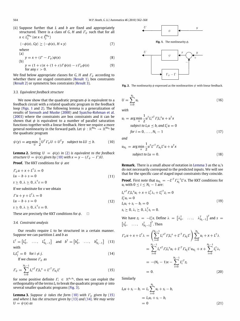
We now show that the quadratic program φ is equivalent to afeedback circuit with a related quadratic program in the feedbackloop (Figs. 1 and 2). The following lemma is a generalization ofresults of Soroush and Muske (2000) and Syaichu-Rohman et al.(2003) where the constraints are box constraints and it can beshown that φ is equivalent to a number of parallel saturationfunctions together with a linear feedback. Here we require a moregeneral nonlinearity in the forward path. Let ψ : RNnu → RNnu bethe quadratic program

ψ(y) = argminU

12UTΓψU + UTy subject to LU � b. (10)

Lemma 2. Setting U = φ(y) in (2) is equivalent to the feedbackstructure U = ψ(x) given by (10) with x = y− (Γψ − Γ )U.

Proof. The KKT conditions for ψ are

Γψu+ x+ LTλ = 0Lu− b+ s = 0

s � 0, λ � 0, λT s = 0

(11)

If we substitute for xwe obtain

Γ u+ y+ LTλ = 0Lu− b+ s = 0

s � 0, λ � 0, λT s = 0.

(12)

These are precisely the KKT conditions for φ. �

3.4. Constraint analysis

Our results require L to be structured in a certain manner.Suppose we can partition L and b as

LT =[LT0, . . . , LTNL−1

]and bT =

[bT0, . . . , bTNL−1

](13)

with

LiLTj = 0 for i 6= j. (14)If we choose Γψ as

Γψ =

NL−1∑i=0

LioTΓiLio + Lc

TΓNLL

c (15)

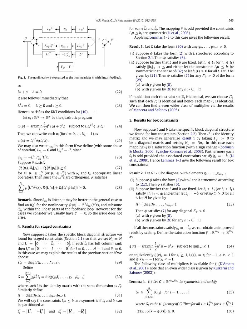
for some positive definite Γi ∈ Rni,ni , then we can exploit theorthogonality of the terms Li to break the quadratic programψ intoseveral smaller quadratic programs (Fig. 3).

Lemma 3. Suppose ψ takes the form (10) with Γψ given by (15)and where L has the structure given by (13) and (14). We may writeU = ψ(x) as

Fig. 1. The nonlinearity φ.

Fig. 2. The nonlinearity φ expressed as the nonlinearities ψ with linear feedback.

U =NL∑i=0

ui (16)

with

ui = argminu

12uT Lio

TΓiLiou+ uT x

subject to Liu � bi and Lci u = 0

for i = 0, . . . ,NL − 1 (17)

and

uNL = argminu12uT Lc TΓNLL

cu+ uT x

subject to Lu = 0. (18)

Remark. There is a small abuse of notation in Lemma 3 as the ui’sdo not necessarily correspond to the predicted inputs. We will seethat for the specific case of staged input constraints they coincide.

Proof. First note that uNL = −Lc TΓ −1NL L

cx. The KKT conditions forui with 0 ≤ i ≤ NL − 1 are:

LioTΓiLioui + x+ LTi λi + L

ciT zi = 0

Lci ui = 0Liui + si − bi = 0

si � 0, λi � 0, λTi si = 0.

(19)

We have zi = −Lci x. Define λ =[λT0, . . . , λTNL−1

]Tand s =[

sT0, . . . , sTNL−1]T. Then

Γψu+ x+ LTλ =

(NL−1∑i=0

LioTΓiLio + Lc

TΓNLL

c

)NL∑i=0

ui + x+ LTλ

=

NL−1∑i=0

LioTΓiLioui + Lc

TΓNLL

cuNL + x+NL−1∑i=0

LTi λi

= −(NL − 1)x−NL−1∑i=0

LciT zi

= 0. (20)

Similarly

Liu+ si − bi = LiNL∑i=0

ui + si − bi

= Liui + si − bi= 0 (21)

W.P. Heath, G. Li / Automatica 46 (2010) 562–568 565

Fig. 3. The nonlinearity φ expressed as the nonlinearities θi with linear feedback.

so

Lu+ s− b = 0. (22)

It also follows immediately that

λT s = 0, λ � 0 and s � 0. (23)

Hence u satisfies the KKT conditions for (10). �

Let θi : Rni → Rni be the quadratic program

θi(p) = argminq

12qTΓiq+ qTp subject to LiLio

Tq � bi. (24)

Then we can write each ui (for i = 0, . . .NL − 1) as

ui(x) = LioTθi(Liox). (25)

We may also write uNL in this form if we define (with some abuseof notation) LNL = 0 and LNL

o= Lc , since

uNL = −Lc TΓ −1NL L

cx. (26)Suppose θi satisfy〈θi(pi), Ri[pi] + Qi[θi(pi)]〉 ≥ 0 (27)for all pi ∈ L

ni2 (or pi ∈ l

ni2 ) with Ri and Qi appropriate linear

operators. Then since the Lio’s are orthogonal, ψ satisfiesNL∑i=0

gi⟨Lioψ(x), Ri[Liox] + Qi[Lioψ(x)]

⟩≥ 0. (28)

Remark. Since θNL is linear, it may be better in the general case tofind an IQC for the nonlinearity ψ(x) − Lc T θNL(L

cx), and subsumeθNL within the linear parts of the feedback loop. However for thecases we consider we usually have Lc = 0, so the issue does notarise.

4. Results for staged constraints

Now suppose L takes the specific block diagonal structure wefound for staged constraints (Section 2.1), so that we set NL = Nand Li =

[0 · · · Li · · · 0

]. If each Li has full column rank

then Lio =[0 · · · I · · · 0

]for i = 0, . . . ,N − 1 and Lc = 0.

In this case wemay exploit the results of the previous section if wechooseΓψ = diag(Γ0, . . . ,ΓN−1). (29)Define

G =N−1∑i=0

giLTi Li = diag(g0I0, . . . , gN−1IN−1) (30)

where each Ii is the identity matrix with the same dimension as Γi.Similarly defineH = diag(h0I0, . . . , hN−1IN−1). (31)We will say the constraints Liu � bi are symmetric if Li and bi canbe partitioned as

LTi =[LTi , −L

Ti

]and bTi =

[bTi , −b

Ti

](32)

for some Li and bi. The mapping θi is odd provided the constraintsLiu � bi are symmetric (Li et al., 2008).Applying Lemmas 1–3 to this case gives the following result:

Result 1. Let G take the form (30) with any g0, . . . , gN−1 > 0.

(i) Suppose φ takes the form (2) with L structured according toSection 2.1. Then φ satisfies (6).

(ii) Suppose further that L and b are fixed. Let hi ∈ L1 (or hi ∈ l1)satisfy ‖hi‖1 < gi and either let the constraints Liu � bi besymmetric in the sense of (32) or let hi(t) ≥ 0 for all t . LetH begiven by (31). Then φ satisfies (7) for any Γψ > 0 of the form(29)(a) with y given by (8),(b) with y given by (9) for any ε > 0. �

If in addition each constraint set Ui is identical, we can choose Γψsuch that each Γi is identical and hence each map θi is identical.We can then find a even wider class of multiplier via the resultsof Mancera and Safonov (2005).

5. Results for box constraints

Now suppose L and b take the specific block diagonal structurewe found for box constraints (Section 2.2). Then Lo is the identitymatrix and we may generalize Result 1 by taking Γψ > 0 tobe a diagonal matrix and setting NL = Nnu. In this case eachmapping θi is a saturation function (with a sign change) (Soroush& Muske, 2000; Syaichu-Rohman et al., 2003). Furthermore eachθi is odd provided the associated constraints satisfy bi = −bi (Liet al., 2008). Hence Lemmas 1–3 give the following result for boxconstraints:

Result 2. Let G > 0 be diagonal with elements g0, . . . , gNnu−1.

(i) Suppose φ takes the form (2) with L and b structured accordingto (2.2). Then φ satisfies (6).

(ii) Suppose further that L and b are fixed. Let hi ∈ L1 (or hi ∈ l1)satisfy ‖hi‖1 < gi and either let bi = −bi or let hi(t) ≥ 0 for allt . Let H be given by

H = diag(h0, . . . , hNnu−1). (33)

Then φ satisfies (7) for any diagonal Γψ > 0(a) with y given by (8),(b) with y given by (9) for any ε > 0. �

If all the constraints satisfy bi = −bi, we can obtain an improvedresult by scaling. Define the saturation function ξ : RNnu → RNnuas

ξ(x) = argminu

12uTu− uT x subject to ‖u‖∞ ≤ 1 (34)

or equivalently ξ(x)i = 1 for xi ≥ 1, ξ(x)i = xi for −1 < xi < 1and ξ(x)i = −1 for xi ≤ −1.The following class of multipliers is available for ξ (D’Amato

et al., 2001) (note that an even wider class is given by Kulkarni andSafonov (2002)).

Lemma 4. (i) Let G ∈ RNnu,Nnu be symmetric and satisfy

Gii ≥n∑

j=1,j6=i

|Gi,j| for i = 1, . . . , n (35)

where Gij is the (i, j) entry of G. Then for all x ∈ LNnu2 (or x ∈ lNnu2 ),

〈ξ(x),G [x− ξ(x)]〉 ≥ 0. (36)

566 W.P. Heath, G. Li / Automatica 46 (2010) 562–568

(ii) Let H(t) ∈ RNnu,Nnu denote a symmetric matrix-valued functionwith entries hi,j in L1 (or l1), and let G ∈ RNnu,Nnu be symmetricand satisfy

Gii ≥n∑

j=1,j6=i

|Gi,j| +n∑j=1

‖Hij‖1 for i = 1, . . . , n. (37)

Then for all x ∈ LNnu2 (or x ∈ lNnu2 )(a)〈ξ(x),Gx〉 ≥ 〈ξ(x),H ∗ x〉 . (38)

(b) For any ε > 0,〈ξ(x),G [(1+ ε)x− ξ(x)]〉≥ 〈ξ(x),H ∗ [(1+ ε)x− ξ(x)]〉 . (39)

Proof. See D’Amato et al. (2001). �

Define also

N = diag(b0, . . . , bNnu−1). (40)

Then ψ defined in (10) can be written

ψ(y) = −Nξ(N−1Γ −1ψ y). (41)

Hence:

Lemma 5. Setting U = φ(y) in (2) is equivalent to the feedbackstructure U = −Nξ(N−1Γ −1ψ x) given by (10) with x = y − (Γψ −Γ )U. �

Lemmas 4 and 5 allow us to give a more general case ofmultipliers for the case where there are only symmetric fixed boxconstraints:

Result 3. (i) Suppose φ takes the form (2) where L and b definefixed symmetric box constraints−bi ≤ Ui ≤ bi. Let N be givenby (40). Let G ∈ RNnu,Nnu be symmetric and satisfy (35) and letΓψ > 0 be diagonal. Define

G = N−1GN−1Γ −1ψ . (42)

Then φ satisfies (6).(ii) Let H(t) ∈ RNnu,Nnu denote a symmetric matrix-valued func-tion with entries hi,j in L1 (or l1), and let G ∈ RNnu,Nnu be asymmetric matrix satisfying (37). Let N be given by (40). LetΓψ > 0 be diagonal. Define

G = N−1GN−1Γ −1ψ and H = N−1HN−1Γ −1ψ . (43)

Then φ satisfies (7)(a) with y given by (8),(b) with y given by (9) for any ε > 0. �

6. An illustrative example for staged constraints

In this section, we use a simple numerical example to illustratehow the results can be applied to the stability analysis of MPC.Consider a two-input four-state discrete linear plant given by

xt+1 = Axt + But with

A = diag(0.21, 0.93, 0.52, 0.26

),

B =[1 1 0 00 0 1 1

]T. (44)

We assume full state information is available. The plant iscontrolled by an MPC law with cost function

J =12‖xN‖2P +

12

N−1∑i=1

‖xi‖2Q +12

N−1∑i=0

‖ui‖2R (45)

where the input horizon (N − 1) = 2 and the weighting matricesare Q = I and R = kI for some k > 0. The weighting matrix P isgiven as the solution of the discrete algebraic Riccati equation

P = ATPA− ATPB(BTPB+ R)−1BTPA+ Q . (46)

The MPC cost function (45) can be expressed as (e.g. Maciejowski,2002).

JI(U) =12UT (R+ ΦT PΦ)U + UTΦT PΛxt (47)

with

P = diag(Q ,Q , P), R = diag(R, R, R)

Φ =

BAB BA2B AB B

, Λ =

AA2A3

(48)

The input is expressed as ui = [u(1)i , u

(2)i ]

T . Suppose that thissystem is subject to the input constraints of the form |u(1)i | ≤ 1,|u(2)i | ≤ 1 and |u

(1)i + u

(2)i | ≤ 1 with i = 0, . . . ,N − 1. These can

be expressed as Liui � bi with

Li =[1, −1, 0, 0, 1, −10, 0, 1, −1, 1, −1

]Tbi =

[1, 1, 1, 1, 1, 1

]T.

(49)

Hence the constraints for the whole horizon can be expressedas Lu � bwith

L = diag(L0, L1, L2) and bT =[bT0, bT1, bT2

]. (50)

Let I2 denote the 2× 2 identity matrix. We have:

L0 =[L0 0 0

], L1 =

[0 L1 0

], L2 =

[0 0 L2

]Lc0 =

[0 I2 00 0 I2

], Lc1 =

[I2 0 00 0 I2

], Lc2 =

[I2 0 00 I2 0

]L0o =

[I2 0 0

], L1o =

[0 I2 0

], L2o =

[0 0 I2

] (51)If we set Γψ = I in (10) then ψ can be written as

ψ(x) =2∑i=0

ui(x) (52)

with

ui(x) = argminui

12uTi ui + u

Ti x

subject to Liui � biand Lci ui = 0. (53)

We can write this as

ψ(x) =[θ0(x0)T , θ1(x1)T , θ2(x2)T

]T (54)

where

θi(xi) = argminqi

12qTi qi + q

Ti xi

subject to Liqi � bi (55)

with L and b given by (49), and where x is partitioned as

x =[xT0, xT1, xT2

]T. (56)

For the sake of this illustration, wewill compare the applicationof Lemma 1, part (i) with the application of Result 1, part (i).Because the constraints are fixed, it would also be possible to apply

W.P. Heath, G. Li / Automatica 46 (2010) 562–568 567

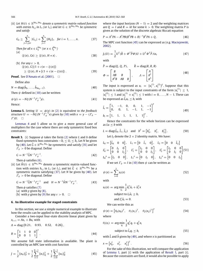
Fig. 4. The closed-loop system.

Lemma 1, part (ii) and Result 1, part (ii). In fact, because the threesets of staged constraints are identical, it would also be possible toextend Result 1 using the results of Mancera and Safonov (2005).Lemma 1, part (i) gives the inequality⟨−φ(x), x+ (R+ ΦT PΦ)φ(x)

⟩≥ 0. (57)

For g0, g1, g2 > 0, define

G = diag(g0I2, g1I2, g2I2). (58)

Result 1, part (i) gives the inequality⟨−φ(x),Gx+ G(R+ ΦT PΦ)φ(x)

⟩≥ 0. (59)

Define Gx(z) = (zI − A)−1B and

M(z) = ΦT PΛGxE ∼[AM BMCM DM

]. (60)

The closed-loop system can then be described as the lineartime invariant transfer function M(z) in feedback with the staticnonlinearity φ(.) (see Fig. 4). Standard IQC theory (Megretski &Rantzer, 1997) gives system stability if the following inequality canbe satisfied[M(ejω)I

]TΠφ

[M(ejω)I

]≤ −εI, ∀ω ∈ [−π, π] (61)

with some ε > 0. Here Πφ is derived from Lemma 1, part (i) orResult 1, part (i) via Eq. (57) or (58) respectively as from Lemma 1:

Πφ =

[0 −I−I −2(R+ ΦT PΦ)

](62)

or from Result 1:

Πφ =

[0 −G−G −(R+ ΦT PΦ)G− G(R+ ΦT PΦ)

]. (63)

By the KYP lemma, the above inequality can be converted intothe following LMI[ATMPMAM − PM ATMPMBMBTMPMAM BTMPMBM

]+ Πφ ≤ −tI, (64)

for some t > 0 and with PM = PTM > 0 and

Πφ =

[CM DM0 I

]TΠφ

[CM DM0 I

]. (65)

Recall that the input weighting is R = kI . We know (Heath& Wills, 2005) that for k sufficiently big the closed-loop systemis stable. Exploiting existing results (Lemma 1) we find that theclosed-loop system is stable for k ≥ 7.9. Exploiting the results ofthis paper (Result 1) we find the closed-loop system is guaranteedstable for all k > 0.

7. Conclusion

For input-constrained MPC the nonlinearity in the controllersatisfies certain IQCs. We have shown that it is possible togeneralize the class of IQCs for MPC with only either staged inputconstraints of the form ui ∈ Ui where eachUi is a convex polytope.The results are derived by considering feedback structures torepresent the nonlinearity. The class may be further generalizedwhen there are only box input constraints.We have demonstrated with a simple numerical state feedback

example that the results may lead to considerable reduction ofconservativeness in the stability analysis of linear fixed horizoninput-constrainedMPC. Themultipliersmay be combinedwith theanalysis of Heath et al. (2006, 2005) to reduce the conservativenessof both nominal and robust stability analysis of input-constrainedoutput feedback MPC.

References

D’Amato, F. J., Rotea, M. A., Megretski, A. V., & Jönsson, U. T. (2001). New results foranalysis of systems with repeated nonlinearities. Automatica, 37(5), 739–747.

Heath, W. P. (1996). Orthogonal functions for cross-directional control of web-forming processes. Automatica, 32(2), 183–198.

Heath, W.P., Li, G., Wills, A.G., & Lennox, B. (2006). The robustness of input con-strained model predictive control to infinity-norm bound model uncertainty.In ROCOND06, 5th IFAC symposium on robust control design, Toulouse, July 5–7.

Heath, W.P., & Wills, A.G. (2005). The inherent robustness of constrained linearmodel predictive control. In 16th IFAC world congress, Prague, July 4–8.

Heath, W. P., & Wills, A. G. (2007). Zames-Falb multipliers for quadraticprogramming. IEEE Transactions on Automatic Control, 52(10), 1948–1951.

Heath, W. P., Wills, A. G., & Akkermans, J. A. G. (2005). A sufficient condition forthe stability of optimizing controllers with saturating actuators. InternationalJournal of Robust and Nonlinear Control, 15, 515–529.

Hill, D. J., & Moylan, P. J. (1977). Stability results for nonlinear feedback systems.Automatica, 13, 377–382.

Kulkarni, V. V., & Safonov, M. G. (2002). All multipliers for repeated monotonenonlinearities. IEEE Transactions on Automatic Control, 47(7), 1209–1212.

Li, G., Heath, W.P., & Lennox, B. (2007). An improved stability criterion for a class ofLur’e systems. In IEEE conference on decision and control, New Orleans, USA, Dec12–14.

Li, G., Heath,W. P., & Lennox, B. (2008). Concise stability conditions for systemswithstatic nonlinear feedback expressed by a quadratic program. IET Control Theoryand Applications, 2(7), 554–563.

Løvaas, C., Seron, M. M., & Goodwin, G. C. (2008). Robust output-feedback modelpredictive control for systems with unstructured uncertainty. Automatica, 44,1933–1943.

Maciejowski, J. M. (2002). Predictive control with constraints. Harlow, Essex: PearsonEducation Limited.

Magni, L., & Scattolini, R. (2007). Robustness and robust design ofMPC for nonlinearsystems. In R. Findeisen, F. Allgöwer, & L. Biegler (Eds.), Assessment and futuredirections of NMPC (pp. 239–254). Berlin: Springer-Verlag.

Mancera, R., & Safonov, M. G. (2005). All stability multipliers for repeated MIMOnonlinearities. Systems and Control Letters, 54(4), 389–397.

Mayne, D. Q., Rawlings, J. B., Rao, C. V., & Scokaert, P. O.M. (2000). Constrainedmodelpredictive control: Stability and optimality. Automatica, 36, 789–814.

Megretski, A., & Rantzer, A. (1997). System analysis via integral quadraticconstraints. IEEE Transactions on Automatic Control, 42, 819–830.

Muske, K. R., & Rawlings, J. B. (1993). Model predictive control with linear models.AIChE Journal, 39(2), 262–287.

Primbs, J. A. (2001). The analysis of optimization based controllers. Automatica, 37,933–938.

Qin, S. J., & Badgwell, T. A. (2003). A survey of industrial model predictive controltechnology. Control Engineering Practice, 11, 733–764.

Soroush, M., & Muske, K. R. (2000). Analytical model predictive control. In F.Allgöwer, & A. Zheng (Eds.), Nonlinear model predictive control (pp. 163–179).Basel: Birkhäuser Verlag.

Syaichu-Rohman, A., Middleton, R.H., & Seron, M.M. (2003). A multivariablenonlinear algebraic loop as a QP with application to MPC. In European controlconference, Cambridge, September 1–4.

Van Antwerp, J. G., Featherstone, A. P., Braatz, R. D., & Ogunnaike, B. A. (2007). Cross-directional control of sheet and film processes. Automatica, 43, 191–211.

Wills, A. G., Bates, D., Fleming, A. J., Ninness, B., & Moheimani, S. O. R. (2008). Modelpredictive control applied to constraint handling in active noise and vibrationcontrol. IEEE Transactions on Control Systems Technology, 16(1), 3–12.

568 W.P. Heath, G. Li / Automatica 46 (2010) 562–568

W.P. Heath is a Senior Lecturer at the Control SystemsCentre, School of Electrical and Electronic Engineering,University of Manchester, UK. He received a B.A. inMathematics from Cambridge University in 1987, andboth an M.Sc. and a Ph.D. from UMIST in 1989 and 1992respectively. He was with Lucas Automotive from 1995to 1998 and was a Research Academic at the Universityof Newcastle, Australia from 1998 to 2004. His interestsinclude constrained control and system identification.

Guang Li received his B.E. degree in Automatic Control andM.Sc. degree in Control Theory and Control Engineering,from the University of Science and Technology Beijing, in2000 and 2003 respectively. He received his Ph.D. degreefrom the Control Systems Centre, the University ofManch-ester in 2007. He is currently a postdoctoral researcher atthe Advanced Control and Test Laboratory in the Univer-sity of Bristol. His research interests includemodel predic-tive control, robust control, nonlinear systems and controlapplications.