multiplicative quaternion extended kalman filtering for ...the prediction step of the kalman...
TRANSCRIPT

Multiplicative Quaternion Extended Kalman Filtering for
Nonspinning Guided Projectiles
by James M. Maley
ARL-TR-6503 July 2013
Approved for public release; distribution is unlimited.

NOTICES
Disclaimers The findings in this report are not to be construed as an official Department of the Army position unless so designated by other authorized documents. Citation of manufacturer’s or trade names does not constitute an official endorsement or approval of the use thereof. Destroy this report when it is no longer needed. Do not return it to the originator.

Army Research Laboratory Aberdeen Proving Ground, MD 21005-5066
ARL-TR-6503 July 2013
Multiplicative Quaternion Extended Kalman Filtering for Nonspinning Guided Projectiles
James M. Maley
Weapons and Materials Research Directorate, ARL Approved for public release; distribution is unlimited.

ii
REPORT DOCUMENTATION PAGE Form Approved OMB No. 0704-0188
Public reporting burden for this collection of information is estimated to average 1 hour per response, including the time for reviewing instructions, searching existing data sources, gathering and maintaining the data needed, and completing and reviewing the collection information. Send comments regarding this burden estimate or any other aspect of this collection of information, including suggestions for reducing the burden, to Department of Defense, Washington Headquarters Services, Directorate for Information Operations and Reports (0704-0188), 1215 Jefferson Davis Highway, Suite 1204, Arlington, VA 22202-4302. Respondents should be aware that notwithstanding any other provision of law, no person shall be subject to any penalty for failing to comply with a collection of information if it does not display a currently valid OMB control number. PLEASE DO NOT RETURN YOUR FORM TO THE ABOVE ADDRESS. 1. REPORT DATE (DD-MM-YYYY)
July 2013 2. REPORT TYPE
Final 3. DATES COVERED (From - To)
October 2012–December 2012 4. TITLE AND SUBTITLE
Multiplicative Quaternion Extended Kalman Filtering for Nonspinning Guided Projectiles
5a. CONTRACT NUMBER
5b. GRANT NUMBER
5c. PROGRAM ELEMENT NUMBER
6. AUTHOR(S)
James M. Maley 5d. PROJECT NUMBER
AH80 5e. TASK NUMBER
5f. WORK UNIT NUMBER
7. PERFORMING ORGANIZATION NAME(S) AND ADDRESS(ES)
U.S. Army Research Laboratory ATTN: RDRL-WML-F Aberdeen Proving Ground, MD 21005-5066
8. PERFORMING ORGANIZATION REPORT NUMBER
ARL-TR-6503
9. SPONSORING/MONITORING AGENCY NAME(S) AND ADDRESS(ES)
10. SPONSOR/MONITOR’S ACRONYM(S) 11. SPONSOR/MONITOR'S REPORT NUMBER(S)
12. DISTRIBUTION/AVAILABILITY STATEMENT
Approved for public release; distribution is unlimited.
13. SUPPLEMENTARY NOTES
14. ABSTRACT
The problem of estimating the attitude, velocity, and position states of a slow to nonspinning, gun-launched projectile is addressed through the use of an extended Kalman filter (EKF). The EKF is constructed using an error-state mechanization similar to those used in traditional inertial navigation applications, although the kinematics are simplified by assuming the Earth-fixed reference frames used for tactical applications are inertial. The advantages of using quaternions rather than Euler angles to represent projectile attitude are discussed, and the use of multiplicative quaternion error states is given detailed attention as this leads to fundamental differences from most other extended Kalman filter implementations that tend to assume additive error states. The measurements and heuristic information available for most projectile applications are incorporated into the EKF. Two sets of simulation results involving a direct-fire system and an indirect-fire system are presented. 15. SUBJECT TERMS
Kalman filter, EKF, projectile, navigation, state estimation, inertial, magnetometers
16. SECURITY CLASSIFICATION OF: 17. LIMITATION OF ABSTRACT
UU
18. NUMBER OF PAGES
48
19a. NAME OF RESPONSIBLE PERSON James M. Maley
a. REPORT
Unclassified b. ABSTRACT
Unclassified c. THIS PAGE
Unclassified 19b. TELEPHONE NUMBER (Include area code) 410-306-0814
Standard Form 298 (Rev. 8/98) Prescribed by ANSI Std. Z39.18

iii
Contents
List of Figures iv
Acknowledgments vi
1. Introduction 1
2. Conventions 4
3. IMU Integration with Quaternions 6
4. Error State Formulation 8
5. Process Noise Measurement 13
6. Projectile Measurement Models 15
6.1 Vector Measurements ....................................................................................................15
6.2 Angle Measurements .....................................................................................................16
6.3 Position and Velocity Measurements ............................................................................17
7. Kalman Filtering Implementation 19
8. Simulation Results 22
8.1 Direct-Fire Application .................................................................................................23
8.2 Indirect-Fire Application ...............................................................................................26
9. Conclusions and Future Work 31
10. References 33
Appendix A. Projectile CG Offset 35
Appendix B. Average Quaternion 37
Distribution List 39

iv
List of Figures
Figure 1. Projection of the magnetic field vector in inertial (i) coordinates into the body-fixed (b) frame as measured by magnetometers for a rolling projectile .............................................1
Figure 2. Coordinate system definitions. .........................................................................................4
Figure 3. U.S. Army/Navy standard finner. ...................................................................................23
Figure 4. Direct-fire small-angle errors. ........................................................................................24
Figure 5. Direct-fire gyro-bias errors. ............................................................................................25
Figure 6. Direct-fire magnetometer-bias errors. ............................................................................25
Figure 7. Indirect-fire trajectory. ...................................................................................................26
Figure 8. Indirect-fire angle errors. ................................................................................................28
Figure 9. Indirect-fire velocity errors. ............................................................................................28
Figure 10. Indirect-fire position errors...........................................................................................29
Figure 11. Indirect-fire gyro-bias errors. .......................................................................................29
Figure 12. Indirect-fire accelerometer-bias errors. ........................................................................30
Figure 13. Indirect-fire magnetometer-bias errors. ........................................................................30

v
List of Tables
Table 1. Kalman filter multitasking schedule. ...............................................................................19
Table 2. Direct-fire initial conditions. ............................................................................................23
Table 3. Direct-fire EKF parameters. ............................................................................................24
Table 4. Indirect-fire initial conditions. .........................................................................................26
Table 5. Indirect-fire EKF parameters. ..........................................................................................27

vi
Acknowledgments
The simulation results leverage the aerodynamic modeling work done by Dr. Frank Fresconi, and the simulink implementation of the projectile flight dynamics, flight control, and guidance laws by Dr. Fresconi, Dr. Mark Ilg, and me, for other research and development projects. I would also like to thank them for their helpful advice and comments.

1
1. Introduction
The primary motivation for this work is to create a general framework for estimating the attitude, velocity, and position states for roll-controlled, guided projectiles for which assumptions about the projectile dynamics may not be valid. Guided projectiles could potentially offer several strategic advantages to the Warfighter by reducing the miss distance, shaping the terminal trajectory, and/or homing to moving targets. While guidance solutions exist for both fin-stabilized and spin-stabilized spinning projectiles, nonspinning projectiles are able to achieve more lateral acceleration for conducting more effective maneuvers than their spinning counterparts (1). The challenge with nonspinning projectiles is that they don’t benefit from the added observability provided from a predictable spin rate. The “slowly varying spin rate” assumption is often used to correct for sensor biases, either directly (2, 3) or indirectly (4). As a simple example, consider the output of a radial magnetometer as depicted in figure 1. The spinning of the round makes it fairly easy to separate a magnetometer sensor bias from the roll angle with respect to the magnetic field vector because the output signal is periodic. This can either be accomplished with empirical routines such as peak finding, or with a linear state estimator by augmenting the projectile state vector with magnetometer bias states that are modeled as constants. If the projectile stops rolling, this continuous observability goes away, and the estimator must rely much more heavily on the process models to account for the uncertainty in attitude and sensor errors.
Figure 1. Projection of the magnetic field vector in inertial (i) coordinates into the body-fixed (b) frame as measured by magnetometers for a rolling projectile
To increase the fidelity of the attitude estimator process model, the propagation equations used in the prediction step of the Kalman filtering process are based on the output of an inertial measurement unit (IMU) rather than a projectile-specific dynamic model. While the dynamic model predictions may still be useful as a heuristic measurement, a dynamic model is usually an approximation of the true dynamics. Errors in the prediction quality are usually approximated by
2
Gaussian white noise acting as a random input to the dynamic system. Since this noise is only an artifact of mathematical convenience rather than a true physical phenomenon, it cannot be measured and is usually used as a tuning parameter. When using kinematics driven by IMU output as the process model, the statistics of the gyroscope and accelerometer noise are measureable, and can be easily incorporated into an extended Kalman filtering framework. A realistic IMU typically has its own sources of modeling error due to sensor calibration errors, non-linearity, cross-axis sensitivity, g-sensitivity, misalignment, etc., which can be either modeled or approximated by increasing the covariance of the process noise.
In the past, both dynamic models (5) and kinematic models (6) have been used as process models for projectile Kalman filters, as well as combinations of the two (7). There have been practical concerns with using an IMU on a projectile, the first of which is the availability of sensors that are capable of measuring the spin rate of a projectile. On a spin-stabilized projectile spinning in the neighborhood of 300 Hz, this is still the case. However, in recent years, micro-electromechanical system (MEMS) gyroscopes have been able to measure the spin-rates of fin-stabilized projectiles such as mortars, which typically spin at rates in the neighborhood of 20 Hz. It is assumed that any nonspinning projectile will not be de-spun from any rate higher than that of typical fin-stabilized projectiles, if indeed it needs to be de-spun at all. The other concern with using IMUs on gun-launched projectiles is the tradeoff between affordability, durability, and performance. Automotive-grade MEMS components have been used in the harsh gun-launch environment for years, and MEMS technology has generally demonstrated its survivability and affordability.
There are still some challenges with MEMS components, however. In the past, sensor bias changes have been observed following the launch event, and most inertial sensors either saturate or temporarily malfunction during the actual launch event although they recover milliseconds after leaving the gun barrel. This leads to an inertial navigation challenge that is particular to gun-launched munitions: the full or partial loss of initial conditions immediately following gun launch. The final concern is sensor quality. The environmental and cost restrictions prohibit the use of most navigation grade or even tactical-grade IMUs used in other applications. However, the flight times of guided munitions are very short, so random walk due to relatively poor noise performance is not as much of a concern as determining calibration and initial condition errors imposed by gun launch. In addition, the MEMS industry is still making progress in improving the noise performance, linearity, temperature stability, cross-axis sensitivity, and vibration rejection of their products, and will likely continue to do so for some time. Therefore, at the very minimum a framework should be in place for evaluating these components for projectile state estimation as they improve.
The choice of attitude representation is an important one. Both quaternions and direction cosine matrices (DCMs) are common in aerospace applications. Quaternions seem to be used in the majority of attitude estimators, because they have fewer elements to store in memory than a DCM, and they are easier to normalize. Euler angles typically don’t see much use outside of

3
projectile applications, because Euler angles can become discontinuous when representing certain orientations and their propagation equations can become indeterminate (8). Since gun-launched projectiles generally don’t experience a wide range of heading angles, this has not a primary concern. The other major advantage of quaternions (or DCMs) over Euler angles is their propagation equations are linear with respect to the quaternion and only depend on the IMU’s angular velocity. This enables much more effective use of the angular rate sensors, as described in section 3 of this report.
A secondary motivation for writing this report is to provide a detailed explanation of multiplicative quaternion error-state Kalman filter mechanizations. Although this form of the Kalman filter has been used in space applications since the 1960s (9) and many other applications (10), clear documentation, especially in terms of guided projectiles, has been difficult to find in the literature. Section 2 discusses notation, coordinate systems, and some preliminary quaternion information that should make this report more readable. Section 4 presents a derivation of the error state kinematic equations that parallels those presented in Crassidis and Junkins (11) and Roumeliotis et al. (12), although a different convention for the quaternion definition is used to be consistent with the conventions used in MATLAB* software and Titterton and Weston (8) and Stevens and Kerce (13).
The position and velocity error state kinematics are included for completeness, although in a very simplified form. In the scope of this work, the local Earth-fixed navigation system is treated as inertial, so many aspects of inertial navigation such as Coriolis acceleration, Schuler tuning, and plumb-bob gravity are not covered here.
Section 5 discusses the measurement of the process noise. The measurements commonly available to guided projectiles and the mapping of the error states to the residuals, the differences between the measured sensor outputs and predicted ones, are discussed in section 6. Section 7 discusses how all of the error state modeling can be implemented in a Kalman filter running on a microcontroller with processing delays. Two different guided projectile missions are simulated to examine the performance of a Kalman filter that estimates the attitude, velocity, position, gyro bias, accelerometer bias, and magnetometer bias errors. The first mission is a short range, direct fire mission where a nonspinning round is controlled and guided to a moving target. The second mission is a mortar that is de-spun near apogee and maneuvers to a ground-based target. The simulations and filter performance are discussed in section 8. Finally, section 9 discusses conclusions and the direction of future research.
* MATLAB is a registered trademark of MathWorks, Inc., Natick, MA.
4
2. Conventions
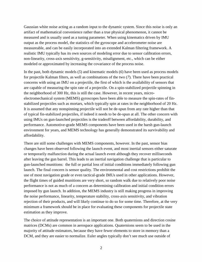
Vectors are defined by lowercase bold script. The terms reference frame and coordinate system are used interchangeably, and all coordinate systems consist of three orthonormal basis vectors; for example, coordinate system a consists of the vectors , ,a a ax y z . A superscript denotes the coordinate system in which the coordinates of the vector are viewed; for example, av is the coordinate of the vector v in the coordinate system a . There are two main reference frames used in this work. The first is the inertial reference ( i -frame). A major simplification used throughout this work is that any reference frame rigidly fixed to the surface of the Earth can be treated as an inertial reference frame for the application to gun-launched projectiles. The inertial frame used here has the z-axis pointing toward the center of the Earth, the x-axis pointed along a level line from the gun toward the initial target location, and the y-axis pointed to the right of the line of fire. The second coordinate system used is the body-fixed reference ( b -frame), which is rigidly attached to the projectile. For the purposes of inertial navigation, it is assumed that the origin of the body frame is located at the location of the accelerometers in the IMU. This prevents the need to account for centripetal and tangential acceleration terms in the integration process. However, the velocity and position states obtained will be those of the IMU and not those of the center of gravity (CG) of the projectile. The two coordinate systems are displayed in figure 2.
Figure 2. Coordinate system definitions.
Body fixed coordinate system
Gun-target line inertial coordinate system
pr
tr Target
bx
iz
ix
iy
by bz

5
To relate the (b-frame) to the (i-frame), we will use quaternion arithmetic. The definition of a quaternion used here has the scalar component as the first element, and the vector component as the second through fourth element, i.e.,
1
2:4
q =
. (1)
The rotation vector μ can also be used to parameterize the quaternion as follows:
1
2:4
cos2
sin2
q
=
μ
q μμμ
. (2)
The quaternion product, denoted⊗ , of any two quaternions p and q is given by (14):
1 1 2:4 2:4
1 2:4 1 2:4 2:4 2:4
p qp q
− ⋅ ⊗ = + + ×
p qp q
q p p q. (3)
The quaternion inverse is defined as the scalar component with the negative of the vector component:
11
2:4
q− = −
. (4)
This quaternion inverse multiplied by the quaternion equals the identity quaternion:
1 1− ⊗ =
q q
0. (5)
Converting a vector from the inertial frame to the body frame can be accomplished with quaternion rotation:
10 0b i
− = ⊗ ⊗
q q
v v. (6)
The same rotation can also be accomplished by converting the quaternion into the direction cosine matrix:
( )b b ii=v C q v , (7)
where:

6
( ) ( ) [ ]22:4 2:4 3 3 1 2:4 2:4 1 2:42 2b T T
i x q q= + − − ×C q q q I q q q . (8)
The general rotation matrix operator ( )biC q reads “transformation from i to b frame coordinates
parameterized by the quaternionq .” The [ ]•× operator denotes the skew-symmetric matrix of a
vector 3∈v , so that multiplying a vector times the matrix is equivalent to taking the cross product of the two vectors, i.e.,
[ ]3 2
3 1
2 1
00
0
v vv vv v
− × = − −
v , (9)
so that [ ]× = ×v w v w . (10)
3. IMU Integration With Quaternions
Integrating the gyro outputs to obtain the projectile attitude is a prerequisite for integrating acceleration to obtain the velocity and position states. The kinematic equations for a quaternion are given by:
01
2 bib
= ⊗
q q
ω . (11)
The vector bibω consists of the body-fixed coordinates of the angular velocity of the body frame
with respect to the inertial reference frame. Equation 3 can be used to reformulate equation 11 as a matrix multiplication:
( )
012
12
b Tib
b bib ib
bib
−=
− ×
=
ωq q
ω ω
Ω ω q
. (12)
It is clear that the quaternion propagation equations are linear with respect to the quaternion. The algorithm presented here is identical to that presented in reference 8 for computing the solution to equation 12 between time steps in a sampled system, although the explanation differs slightly. For the remainder of this section, the reference frame notation b
ibω will be replaced by iteration

7
notation kω , meaning the value of bibω sampled at time k . In this case the solution to equation 12
is given by:
( )11exp2k kt+
= ∆
q Ω ω q . (13)
The value of ω is usually taken to be:
1
2k k−+
=ω ωω . (14)
The incremental rotation vector can be approximated as* t= ∆σ ω . For a given rotation vector, the exact solution for the matrix exponential in equation 13 is given by (8):
( )( ) ( )
( ) ( ) ( ) [ ]3 3
sin 2cos 2
1 2exp2 sin 2 sin 2
cos 22 2
T
x
= − ×
σσ σ
Ω σσ σ
σ σ I σ. (15)
The velocity dynamics are a function of the specific force measured by the accelerometers bf , the gravity vector ig , and the quaternion:
( )i i b ib= +v C q f g . (16)
Using equations 13–15, it is possible to predict what the quaternion will be at the current time step based on angular rate sensor data. Velocity and position are estimated via simple trapezoidal integration, which requires the quaternion at time k to be estimated first. The velocity update is given by:
( ) ( )1 112
i b i bb k k b k k i
k kt− −−
+= + ∆ +
C q f C q fv g v . (17)
The position update is then given by:
112
i ii ik kk kt−
−
+= ∆ +
v vr r . (18)
*There exist higher-fidelity representations of the rotation vector. Bortz (15) derives the rotation vector, its dynamics, and its
relation to the DCM from geometric arguments. It was shown that the rotation vector can be integrated at a high integration rate and then used to update the DCM only when needed, significantly increasing algorithm efficiency. Since then, particularly in Savage (16), several algorithms have been created for computing the rotation vector on digital processors, and how the rotation vector relates to the DCM and quaternion attitude representation. The advantage of using the trapezoidal approximation used here is that calibration corrections can easily be applied after the inertial sensors have been sampled as discussed in more detail in section 7, without needing to retain several samples in memory. The disadvantage is that the approximation will necessitate a faster KF update rate.

8
This algorithm assumes that the specific force in the inertial frame is fairly constant over the update interval. The inertial specific force ( )i i b
b=f C q f , can be computed in terms of the projectile’s acceleration i
cgv and the location of the CG relative to the body frame bcgr :
( ) [ ][ ] [ ]i b i i b i b ib cg b cg b cg= − × × − × −C q f v C ω ω r C ω r g . (19)
Full derivation is given in appendix A.
On a guided projectile, the acceleration of the CG does not usually change dramatically since most projectiles have limited control authority. Mounting the accelerometer triad on the spin axis is strongly advisable, since centrifugal accelerations can be quite large. Algorithms in literature typically don’t use a trapezoidal integration scheme at all but use a combination of incremental velocity, rotation correction, and dynamic integral terms, and potentially more advanced sculling and scrolling compensation algorithms (8, 16). However, for our purposes the algorithm provides a method of post applying calibration corrections and is computationally tractable.
4. Error State Formulation
The integration of the quaternion, velocity, and position states is in reality driven by non-perfect gyroscopes and accelerometers. Therefore, the integrated states are only estimations of the true states. Terms that are estimates are denoted by the ^ over script. The estimated state dynamics are given by:
01ˆ ˆˆ2 b
ib
= ⊗
q q
ω , (20)
( ) ˆˆ ˆˆ i i b ib= +v C q f g , (21)
and ˆ ˆi i=r v . (22)
From this point forward, we will drop the super and subscripts for simplicity. The IMU outputs estimated angular velocity and specific force vectors, which are defined by:
ˆ= + δω ω ω . (23)
ˆ= + δf f f . (24)
The perturbation termsδω andδf can be parameterized by any noise and sensor calibration errors substantial enough to affect the navigation solution.

9
The true quaternion q can be described as the quaternion multiplication of the estimated quaternion q̂ and a small error quaternion δq :
ˆ= ⊗δq q q . (25)
1ˆ −δ = ⊗q q q . (26)
This description is not common in other extended Kalman filtering problems, which typically treat the error terms as additive, i.e., ˆ= + δq q q . The additive error assumption is used in most Kalman filtering texts such as Simon (17) and Gelb (18). Indeed, there are even several quaternion estimators that use this assumption (10). Adding two unit quaternions together does not produce another unit quaternion, which creates a problem that is normally dealt with by gratuitous renormalization. It is possible, but quite complicated, to correctly account for these computational aspects in the error covariance matrix (19). The multiplicative error formulation also has the physical interpretation of applying a small rotation correction. This can easily be shown in the formulation of the composite DCM. Using the conventions in this work, the total DCM is given by:
( ) ( ) ( ) ( )ˆ ˆbi = ⊗δ = δC q C q q C q C q . (27)
Another benefit of the multiplicative error quaternion is that only three terms are needed to parameterize it instead of four. Since the error quaternion represents a small rotation, the rotation vector μ from equation 2 has small magnitude which means that the scalar component of δq is approximately 1 and need not be estimated. The only downside is that the linearization of the processes and measurement equations cannot be accomplished simply by computing Jacobians.
The quaternion error state dynamics are produced by differentiating equation 26 with respect to time:
1 1ˆ ˆ− −δ = ⊗ + ⊗q q q q q . (28)
A substitution for 1ˆ −q can be generated from the fact that 1ˆ ˆ− ⊗q q always produces the identity quaternion, which is constant.
( )1
1 1ˆ ˆ
ˆ ˆ ˆ ˆd
dt
−− −
⊗= ⊗ + ⊗ =
q qq q q q 0 . (29)
1 1 1
1 1
1
ˆ ˆ ˆ ˆ01ˆ ˆ ˆˆ2
01 ˆˆ2
bib
bib
− − −
− −
−
= − ⊗ ⊗
= − ⊗ ⊗ ⊗
= − ⊗
q q q q
q q qω
qω
. (30)

10
Substituting equations 30 and 11 into equation 28 leads to:
1 10 01 1ˆ ˆˆ2 2
0 01 1ˆ2 2
bib
− − δ = ⊗ ⊗ − ⊗ ⊗
δ = δ ⊗ − ⊗δ
q q q q qω ω
q q qω ω
. (31)
Using the definition of the estimated angular velocity (equation 20), this becomes:
0 0 01 1 1ˆ ˆ2 2 2
δ = δ ⊗ − ⊗δ + δ ⊗ δ q q q q
ω ω ω . (32)
The definition of quaternion multiplication can now be applied along with the fact that 1 1qδ = to achieve further simplification:
2:4 2:4 2:4
2:4 2:4 2:4
2:4
2:4 2:4 2:4
ˆ ˆ ˆ1 1 1ˆ ˆ ˆ ˆ ˆ ˆ2 2 2
ˆ0 0 1ˆ ˆ ˆ2
−δ ⋅ ⋅δ −δ ⋅δ δ = + + + δ × − − ×δ δ + δ ×δ
−δ ⋅δ = + δ − ×δ δ + δ ×δ
q ω ω q q ωq
ω q ω ω ω q ω q ω
q ωq ω q ω q ω
. (33)
Since the quaternion error states are assumed to be small in magnitude, the error state dynamics can be approximated by:
2:4 2:41ˆ2
δ ≅ − ×δ + δq ω q ω . (34)
At this point, it is convenient to replace the quaternion error states 2:4δq with a vector of small angles:
2:42= δα q . (35)
The first convenience comes from removing the factor of ½ from equation 34:
ˆ≅ − × + δα ω α ω . (36)
The second convenience comes from the simplification of equation 27. Evaluating equation 8 with δq and assuming products of the terms in 2:4δq are approximately zero results
in ( ) [ ]2:42bi δ ≅ − δ × C q I q . Therefore, the DCM and its inverse can be expressed as:
( ) [ ] ( )ˆb bi i ≅ − × C q I α C q . (37)
( ) ( ) [ ]ˆi ib b ≅ + × C q C q I α . (38)

11
The velocity and position error state dynamics are simpler to derive, since their error states are additive:
ˆδ = −v v v . (39)
ˆδ = −r r r . (40)
The velocity error states propagate according to:
ˆδ = −v v v . (41)
By utilizing equations 21, 24, 38, and 41, an expression for the velocity error state dynamics can be derived:
( ) ( ) ˆˆ ˆi b i bb bδ = + − +v C q f g C q f g ( ) [ ] ( ) ( )ˆ ˆˆ ˆ ˆi b i b
b b δ = + × + δ + − − v C q I α f f g C q f g
( )[ ] ( ) ( ) [ ]ˆˆ ˆ ˆi ii bb b b
δ = × + δ + × δ + δv C q α f C q f C q α f g (42)
Due to the small angle error assumption, it is assumed that
( ) [ ] ( )ˆ ˆi i
b b + × δ ≅ δ C q I α f C q f . (43)
Also, it is assumed for this application that the gravity errorδg is negligible. Therefore, equation 42 can be expressed as a linear system with respect to the error states:
( ) ( )ˆˆ ˆ ii bb b
δ = − × + δ v C q f α C q f . (44)
The position error state dynamics are:
ˆ ˆδ = − = − = δr r r v v v . (45)
The angular rate and specific force error states δω andδf are parametric, and can be used to model sensor calibration or noise terms. The angular rate error model that we will use here is a bias plus noise model:
ˆ ω ω= − −ω ω β η (46)
and ω ω=β υ , (47)
where ωη and ωυ are white random processes with cross-correlations:
( ) ( ) ( ) ( )2TE t diag tω ω ω τ = δ − τ η η σ . (48)
( ) ( ) ( ) ( )2TE t diag tω ω βω τ = δ − τ υ υ σ . (49)

12
The angular rate error term from equations 23 and 46 becomes:
ω ωδ = − −ω β η . (50)
ωδ = −ω υ . (51)
The specific force measurements from the accelerometers are treated in a similar manner:
ˆf f= − −f f β η , (52)
f f=β υ , (53)
and f fδ = − −f β η , (54)
where fη and fυ are white random processes with cross-correlations:
( ) ( ) ( ) ( )2Tf f fE t diag t τ = δ − τ η η σ . (55)
( ) ( ) ( ) ( )2Tf f fE t diag tβ τ = δ − τ υ υ σ . (56)
Magnetometers will be used as measurements in the eventual Kalman filter implementation. The magnetometer is not an inertial sensor, and its error dynamics are uncoupled with the inertial navigation states, but a bias term is still augmented to the total error state vector since some correlation is expected to be introduced by the Kalman filter measurement update equations. The magnetometer bias vector mβ here is treated as a slowly diverging random walk process driven by the noise process mυ with cross correlation:
( ) ( ) ( ) ( )2Tm m mE t diag tβ τ = δ − τ υ υ σ . (57)
m m=β υ . (58)
The total error state vector is now:
{ }TT T T T T Tf mωδ = δ δx α v r β β β . (59)

13
The error state dynamics can be written in state space form:
[ ]( ) ( )
3 3 3 3 3 3 3 3 3 3
3 3 3 3 3 3 3 3
3 3 3 3 3 3 3 3 3 3 3 3
3 3 3 3 3 3 3 3 3 3 3 3
3 3 3 3 3 3 3 3 3 3 3 3
3 3 3 3 3 3 3 3 3 3 3 3
ˆˆˆ ˆi b i
b b
f
m
× × × × ×
× × × ×
× × × × × ×
ω× × × × × ×
× × × × × ×
× × × × × ×
− × − δ − × − δ =
ω 0 0 I 0 0αv C q f 0 0 0 C q 0r 0 I 0 0 0 0β 0 0 0 0 0 0β 0 0 0 0 0 0β 0 0 0 0 0 0
( )3 1
ˆib f
f f
m m
ω
×
ω ω
− δ − δ +
α ηv C q ηr 0β υβ υβ υ
. (60)
This 18-error-state, state-space model will be used for Kalman filter implementation in this work. An important result is that the model is linear and time-varying with respect to the error states. The advantage of this is that when the Kalman filter is implemented in realtime, the state transition matrix can be constructed without knowing the error states at the last measurement time from the information available from the IMU integration. Another advantage of this form is that there are no trigonometric operations involved with its computation. The third advantage is that the model is truly a stochastic system that is driven by white noise sequences that have spectral densities that are either measureable or easily approximated.
5. Process Noise Measurement
From equation 60, the following matrices are defined:
( )
[ ]( ) ( )
3 3
3 3
ˆˆˆ ˆ
ˆˆ ˆ, ,
i b ib b
×
×
− × −
− × − =
ω 0 0 I 0 0
C q f 0 0 0 C q 0
0 I 0 0 0 0F q ω f0 0 0 0 0 00 0 0 0 0 00 0 0 0 0 0
. (61)
( )
( )( ) ( )
( )( )
( )
ˆ
ˆ
ib f
f
m
diag
diag
diag
diag
diag
ω
βω
β
β
−
−
=
σ 0 0 0 0 0
0 C q σ 0 0 0 0
0 0 0 0 0 0G q 0 0 0 σ 0 0
0 0 0 0 σ 0
0 0 0 0 0 σ
. (62)

14
Using these definitions, the error state dynamics can be represented by the following matrix equation:
δ = δ +x F x Gw . (63)
The vector w is a white noise sequence with unity variance and zero mean. The matrix G transforms the white noise sequence into the disturbance vector. Therefore, the uncertainty of the disturbance vector can be represented by:
( )( ) ( )( ) ( )TcE t t τ = δ − τ
Gw Gw Q , (64)
which simplifies to:
( ) ( )
( )( )
( )( )
( )
( )
2
2
2
2
2
f
Tc
f
m
diag
diag
t t tdiag
diag
diag
ω
βω
β
β
δ − τ = δ − τ = δ − τ
σ 0 0 0 0 0
0 σ 0 0 0 0
0 0 0 0 0 0Q GG
0 0 0 σ 0 0
0 0 0 0 σ 0
0 0 0 0 0 σ
. (65)
Representing the process noise as a continuous noise process simplifies filter tuning by making it sample time agnostic. However, discrete time integration leads to different variance growth than continuous time integration. Consider the integration of a scalar random signal. The integration of a continuous white noise signal with spectral amplitude 2
cσ has the transfer function:
( )( ) ( ) cy s
G su s s
σ= = . (66)
Therefore, the variance of the output y at some time t is given by (17):
2 2 2
0 0[ ( )] ( )
t t
c cE y t u v dudv t= σ δ − = σ∫ ∫ . (67)
Consider the integration of a discrete white noise sequence ~ (0, )k dx N σ . If this sequence is integrated with rectangular integration, the output is given by:
1 0( ... )k k ky t x x x−= ∆ + + . (68)

15
The output variance is given by:
21 0 1 0
2 2 2 2 21
2 2 2 2
[ ] [ [ ... ] [ ... ] ]
[ ] ( [ ] [ ] ... [ ])
[ ]
Tk k k k k
k k k o
k d d
E y E t x x x t x x xE y t E x E x E xE y t k t t
− −
−
= ∆ + + ∆ + +
= ∆ + +
= ∆ σ = ∆ σ
. (69)
The standard deviation of the discrete white noise sequence is easily estimated from a short sample of a sensor’s null output, and from it the spectral amplitude can be calculated for an equivalent continuous noise process. Therefore, in this work, the noise amplitudes for the angular rate sensors and accelerometers, 2
ωσ and 2fσ , respectively, are calculated as a function of the
estimated discrete time variance and the integration sample time:
ˆc d tσ = σ ∆ . (70)
The drift-rate terms for the sensor biases are not analytically measured or simulated here. Allan variance analysis reveals the existence of flicker noise, but its measurement, simulation, and effect on a guided projectile’s navigation solution are left as the subject of future work. Therefore, while the sensor noise parameters are measured, the bias drift parameters βωσ , fβσ , and mβσ are chosen as tuning parameters.
6. Projectile Measurement Models
6.1 Vector Measurements
Because of the normal operating conditions for guided projectiles, there are only a few different kinds of measurements available. The most common are vector measurements in which a vector’s coordinates are either known a-priori or measured in both the inertial and body-fixed frames. Since magnetometers are probably the most common vector measurement used by the projectile community, the Earth’s magnetic field vector m will be used to illustrate the mapping of the error states to a vector’s measurement residuals. Assuming the scale factor and misalignment terms are known, the magnetic field vector as measured by the magnetometer is given by:
( )b b ii m m= + +m C q m β η . (71)
That is, the measured bm is the known vector in inertial coordinates im transformed into the body coordinates, plus a body-fixed bias vector mβ and an additive zero-mean white noise term mη . The
residual δm is formed by subtracting the predicted measurement ˆ bm from the actual measurement.

16
The predicted measurement is a function of the current estimated quaternion:
( )ˆ ˆb b ii=m C q m . (72)
Equation 37 can be substituted into equation 71 to get:
[ ] ( )ˆb b ii m m ≅ − × + + m I α C q m β η (73)
The measurement residual is then:
[ ] ( ) ( )ˆ ˆ ˆb b b i b ii m m i − = − × + + − m m I α C q m β η C q m , (74)
which simplifies to a linear mapping of the error states:
( )( ) 3 3ˆb b ii m
m×
δ = × +
αm C q m I η
β . (75)
Another all-weather vector measurement is the projectile’s velocity vector in inertial coordinates iv . This can usually be obtained from an onboard GPS unit or from a reference trajectory or dynamic model depending on the mission specifications. Since most projectiles fly at a fairly low angle of attack, the body fixed coordinates are assumed to be:
{ }0 0Tb b=v v . (76)
The noise in the velocity vector is usually more naturally expressed in inertial coordinates. The measurement residual is given by:
( )ˆi i i bbδ = −v v C q v . (77)
The measured velocity in inertial coordinates can be rewritten in terms of the error states and the noise vector vη :
( ) [ ]ˆi i bb v ≅ + × + v C q I α v η . (78)
This leads to the following linear mapping of the error states to the velocity vector residual:
( )ˆi i bb v δ = − × + v C q v α η (79)
6.2 Angle Measurements
Some measurement sources provide direct measurements of Euler angles. For example, a constellation of thermopile sensors with the appropriate signal processing provides a direct measurement of the roll angleφ from a ZYX Euler angle rotation sequence, except in specific

17
weather conditions (2, 3). Certain computer vision algorithms can use horizon detection to measure both the pitch angleθ as well asφ (20). Arguably, it might not make sense to even be using a quaternion-based attitude representation in this situation, but if quaternions are more suited for the mission requirements it is still simple to use Euler angle measurements. In this case, one would compare the measured Euler angles to the Euler angles computed from the current quaternion prediction to get Euler angle error residuals. That is, for a typical ZYX Euler angle rotation sequence:
ˆφδφ = φ−φ+η , (80)
ˆθδθ = θ−θ+η , (81)
and ˆ
ψδψ = ψ −ψ +η , (82)
where:
( )( )2 2 2 23 4 1 2 1 2 3 4
ˆ ˆ ˆ ˆ ˆ ˆ ˆ ˆ ˆatan2 2 ,q q q q q q q qφ = + − − + . (83)
( )( )( )12 4 1 3
ˆ ˆ ˆ ˆ ˆsin 2 q q q q−θ = − − . (84)
( )( )2 2 2 22 3 1 4 1 2 3 4
ˆ ˆ ˆ ˆ ˆ ˆ ˆ ˆ ˆatan2 2 ,q q q q q q q qψ = + + − − . (85)
A quaternion Kalman filter estimates small rotation angles however, so a mapping must be used between the Euler angle residuals, and small rotation angle error states. Assuming that both Euler angle residuals and error states are small angles, the mapping between the two is identical to the mapping between Euler angle time derivatives and the body-fixed angular rate vector:
( ) ( ) ( ) ( )( ) ( )
( ) ( ) ( ) ( )
ˆ ˆ ˆ ˆ1 sin tan cos tan
ˆ ˆ0 cos sin
ˆ ˆ ˆ ˆ0 sin / cos cos / cos
φ θ φ θ δφ δθ = φ − φ δψ
φ θ φ θ
α
. (86)
When implementing Euler angle measurements, it is very important to make sure that the measured and predicted quantities are in the same quadrant.
6.3 Position and Velocity Measurements
The availability and source of actual position measurements is highly subjective to mission requirements. The mapping from the error states to direct position or velocity residuals is simple:
[ ]ˆr− = δ +r r I r η . (87)

18
[ ]ˆv− = δ +v v I v η . (88)
In reality, the measurements are usually more complicated. If the user has access to the direct GPS pseudo-range and carrier-frequency measurements, it would be more accurate to use the well-known GPS measurement models that include user clock bias. If the user does not have access to the direct receiver outputs but instead is provided with the receiver’s calculated position and velocity estimate, it may be more accurate to measure the errors to construct an auto-regressive or Gauss-Markov error model instead of assuming white noise. In the case of a reference trajectory, it may be beneficial to treat the dynamic model as a random process so that the reference trajectory “measurements” get weighed less and less as the trajectory progresses in time. A simple way to do this is to model the errors in reference trajectory states as three coupled position velocity states driven by random noise:
0 10 0
x zx zref
x zx z
rrvv
−−
−−
δ δ = + δδ
η
. (89)
Deviations from the reference trajectory due to unmodeled disturbances such as wind would be accounted for in the noise term refη which is parameterized by the tuning variable refq :
( ) ( ) ( )2
0 00
Tref ref
refE t t
q
τ = δ − τ
η η . (90)
The measurement covariance at some time later can be calculated from an initial value 0refR and
the tuning variable:
( )( )
( )( )
3 22
0 2
1 1 0 3 20 1 1 2
T
x z x zref ref
x z x z
r t r t t t tE q
v t v t t t t− −
− −
δ δ = + δ δ R
. (91)
This measurement covariance matrix would then be used in the EKF when calculating the gains for the position and velocity measurements.

19
7. Kalman Filtering Implementation
The Kalman filter is eventually intended to be run on an embedded processor. In this work, this is accomplished by discretizing the error state dynamics so that the Kalman filtering equations can be updated at a lower frequency than the integrated states. The integration of the gyroscopes and accelerometers to acquire quaternion, velocity, and position will be updated at a faster rate than the EKF since the integration should require significantly less computing power and delayed feedback can degrade the performance of flight controllers. Assuming some type of multitasking is used, the Kalman filter equations are run at a slower rate with a lower priority as shown in table 1.
Table 1. Kalman filter multitasking schedule.
IMU Integration Time i = EKF Update Time j = 0 Start at 0ˆ −x
1
Measurements 0j=y Kalman Filtering
Calculations Updated 0ˆ j
+=x known
Predict 1ˆ j−=x
1 Integrate ˆ −x from 0ˆ i−=x
2 Integrate ˆ −x from 1ˆ i−=x
3 Integrate ˆ −x from 2ˆ i−=x
4 Integrate ˆ −x from 3ˆ i−=x
5 Integrate ˆ −x from 1j−=x
2
Measurements 0j=y Kalman Filtering
Calculations Updated 1ˆ j
+=x known
Predict 2ˆ j−=x
6 Integrate ˆ −x from 5ˆ i−=x
7 Integrate ˆ −x from 6ˆ i−=x
8 Integrate ˆ −x from 7ˆ i−=x
9 Integrate ˆ −x from 8ˆ i−=x
— Etc. — Etc.

20
The integration of the full states is accomplished using the equations in section 5 and the best known gyroscope, and accelerometer calibrations. The actual Kalman filtering calculations are performed to estimate the error states at the time of the measurements. Each Kalman filter iteration consists of the following five steps:
1. Measurement/Storage
Record the measurements and their covariance values (if time varying) from whatever sources are available. Record the value of integrated full states at this time, as they will be used to form the residuals.
2. Covariance Prediction
The full state prediction comes from the integration task. The a-priori error-state estimate is zero:
ˆ j−δ =x 0 . (92)
An estimate of the a-priori error-state covariance matrix j−P must be predicted from the previous
iteration’s a-posteriori error-state covariance 1j+−P and the error-state dynamics. The matrix F
previously defined in equation 61 can be discretized to form a state transition matrix using the second-order approximation for the matrix exponential:
2 212
t t= + ∆ + ∆Φ I F F . (93)
The values that go into the F matrix are determined from the current a-priori quaternion estimate and IMU outputs, and the previous iteration’s a-posteriori quaternion estimate and IMU outputs. The nonzero terms in F are therefore:
[ ] ( )
( )( ) ( )
( ) ( )
1
1 1
1
ˆ ˆ ˆ / 2
ˆ ˆˆ ˆˆˆ
2ˆ
j j
i b i bb j j b j ji b
b
i i jb b j
−
− +− +
−
− × = − + × − × + − × − × =
− = −
ω ω ω
C q f C q fC q f
C q C q
. (94)
Note that the term 1jj−q is the average quaternion determined from the algorithm in appendix B, as
arithmetic averaging of two rotation transformation matrices violates the orthonormal constraints. The a-priori error state covariance is calculated as:
1T T
j j dE− +− = δ δ = + P x x ΦP Φ Q . (95)
The discrete time process noise covariance matrix dQ is determined from:
( ) ( )0
Tt t td ce e d
∆ −τ −τ= τ∫ F FQ Q . (96)

21
The previous equation can be simplified considerably by assuming that the F matrix is linearized about the conditions ˆˆ 0= =ω f and ( )ˆb
i =C q I . This makes some sense intuitively, works in practice, and is used in reference 11, but an analytical reason why this works is left as a subject of future research. With this simplification and the definition of cQ defined in equation 65 an analytical expression can be determined. With the notational shorthand ( )Λ v meaning a matrix with the elements of the vector v along the diagonal, the analytical expression is:
( ) ( ) ( )
( ) ( ) ( ) ( ) ( )
( ) ( ) ( ) ( ) ( )
( ) ( )
( ) ( ) ( )( )
3 22 2 2
3 4 2 22 2 2 2 2
2 4 3 5 32 2 2 2 2
2 22 2
2 32 2 2
2
3 2
3 8 2 2
2 8 3 20 6
2 2
2 6
f f f f f
f f f f fd
f f f
m
t tt
t t t tt
t t t t t
t t
t t t
t
ω βω βω
β β β
β β β
βω βω
β β β
β
∆ ∆∆ + −
∆ ∆ ∆ ∆
∆ + + −
∆ ∆ ∆ ∆ ∆+ + −
=∆ ∆
−
∆ ∆− − ∆
∆
Λ σ Λ σ 0 0 Λ σ 0 0
0 Λ σ Λ σ Λ σ Λ σ 0 Λ σ 0
0 Λ σ Λ σ Λ σ Λ σ 0 Λ σ 0Q
Λ σ 0 0 Λ σ 0 0
0 Λ σ Λ σ 0 Λ σ 0
0 0 0 0 0 Λ σ
. (97)
3. Evaluate residual mappings
All of the linear maps from the error states to the residuals in section 6 are functions of the current full state vector. In the case of linear Kalman filters, if all of the measurements are uncorrelated the measurements can be processed one at a time with identical results as processing them all at once (17). This adds convenience and reduces computation time since matrix inversion is avoided. To achieve the same effect with an EKF, the measurement maps must all be evaluated using the same a-priori full state estimate.
4. Sequential Kalman filter innovation steps
For each available measurement the following equations steps are taken. All of the residual maps in section 6 can be put into the form:
yδ = δ + ηh x , (98)
where yδ is equal to the actual measurement minus the predicted measurement. The noiseη will have some known covariance 2
yσ . The Kalman gain is then:
( )2
TjT
j y
−
−=
+ σ
P hk
hP h. (99)
The error state vector is updated with the Kalman gain:
ˆ ˆj j y+ −δ = δ + δx x k . (100)

22
The error state covariance matrix is updated next:
( )j j+ −= −P I kh P . (101)
If there are more measurements to be processed, then the a-priori error states and covariance matrix are overwritten as ˆ ˆj j
− +δ = δx x and j j− +=P P before the innovation steps are repeated with the
next measurement.
5. Update the full states and calibration parameters
Using the definitions for each error state as defined in section IV the full state estimate can be updated with the error state estimate. For the quaternion, this amounts to:
1
ˆ ˆ2j j
+ − = ⊗
q q
α. (102)
The position and velocity estimates are updated as:
ˆ ˆj j+ −= + δr r r . (103)
ˆ ˆj j+ −= + δv v v . (104)
The bias estimates for the magnetometer, gyroscopes, and accelerometers are used to correct the calibrations for each sensor, and then set to zero. At this point, the full state estimates are updated at time j , which will have been some distance in the past depending on the speed of the processor. A current full state estimate can be obtained by using the IMU integration equations in section 3 and the outputs of the gyroscopes and accelerometers at time j and the current time. Note that when applying equation 70 to calculate the continuous random walk coefficients, better performance is usually obtained by using the time difference between the current time and time j when this time step is large instead of the integration time step.
8. Simulation Results
To validate some of the models and algorithms presented here, simulations were constructed in a Matlab/Simulink environment that included full six-degree-of-freedom (6-DOF) motion of the projectile as well as the state estimation, guidance, and control algorithms. The simulations are not to provide performance metrics for any specific system, but to demonstrate the basic functionality of the algorithms discussed in this report and discuss some of the problems with guided projectile applications.

23
8.1 Direct-Fire Application
The first system simulation is a low QE guide to hit mission against a moving target. The projectile used was the U.S. Army/Navy standard finner (21–24), which is a fin-stabilized nonspinning round, modified with four canards as shown in figure 3.
Figure 3. U.S. Army/Navy standard finner.
The projectile uses proportional navigation as the guidance law to engage the moving target. The autopilot is a state-feedback controller designed using optimal control techniques (25). The initial conditions for the simulation are shown in table 2.
Table 2. Direct-fire initial conditions.
Quantity Value Units Muzzle velocity 200 m/s Gun elevation 8 deg
Projectile initial position {0 0 0}T m Target initial position {1000 0 0}T m
Target velocity {0 10 0}T m/s Projectile initial angular velocity {2 2 2}T rad/s
The state estimator is only an attitude estimator in this case, as no actual position or velocity measurements are available. The gyros are corrupted by white noise with the same parameters measured from some modified ADXRS300 angular rate sensors, although no flicker or rate-ramp was modeled. Magnetometer measurements are present with the same noise measured from an HMC1043 solid-state magnetometer. It is assumed that relatively large initial biases might be present in the magnetometer due to body-fixed static magnetic fields generated by the projectile itself. The effects of motors and eddy current effects are neglected. No misalignment, scale factor, non-orthogonality, or g-sensitivity errors are modeled for either sensor. In addition to magnetometers, it is assumed that a computer vision horizon detection algorithm produces roll and pitch estimates at 30 Hz. It is also assumed that the computer-vision and EKF processing takes 80% of the update interval (26.7 ms) to complete. It turns out the yaw angleψ is

24
unobservable with this configuration (it is indistinguishable from the x-axis magnetometer bias). To remedy this, a heuristic yaw angle measurement of 0° is used for the first 0.5 s to enable the sensor biases to converge. The EKF parameters are shown in table 3, and errors are illustrated in figures 4–6.
Table 3. Direct-fire EKF parameters.
Quantity Value Units Initial attitude error covariance ( )0TE t = αα diag{100 1 1}2 deg2
Initial gyro bias error covariance ( )0TE tω ω = β β diag{10 10 10}2 (deg/s)2
Initial magnetometer bias error covariance ( )0Tm mE t = β β diag{1 1 1}2 Gauss2
Gyro bias drift covariance ( )2diag βωσ diag{1 1 1}x1e-3 (rad/s/s)2
Magnetometer bias drift covariance ( )2mdiag βσ diag{1 1 1}x1e-3 (Gauss/s)2
Gyroscope noise std. dωσ { 2.0626 2.0626 2.0626 }T deg/s Magnetometer noise std. mdσ {0.0022 0.0022 0.0022}T Gauss Horizon roll/pitch measurement noise std. 1 Deg Quaternion integration rate 500 Hz Kalman filter update rate 30 Hz Earth’s magnetic field in gun-target line coordinates {0.5 0 0}T Gauss
0.5 1 1.5 2 2.5
-202
time (sec)
αx(d
eg)
errorKF 3σ bound
0.5 1 1.5 2 2.5-2
0
2
time (sec)
αy(d
eg)
errorKF 3σ bound
0.5 1 1.5 2 2.5-2
0
2
time (sec)
αz(d
eg)
errorKF 3σ bound
Figure 4. Direct-fire small-angle errors.

25
0.5 1 1.5 2 2.5-10
0
10
time (sec)
β ωx (d
eg/s
)
errorKF 3σ bound
0.5 1 1.5 2 2.5
-505
time (sec)
β ωy (d
eg/s
)
errorKF 3σ bound
0.5 1 1.5 2 2.5
-505
time (sec)
β ωz (d
eg/s
)
errorKF 3σ bound
Figure 5. Direct-fire gyro-bias errors.
0.5 1 1.5 2 2.5-4-2024
x 10-3
time (sec)
β mx (G
)
errorKF 3σ bound
0.5 1 1.5 2 2.5-0.02
00.02
time (sec)
β my (G
)
errorKF 3σ bound
0.5 1 1.5 2 2.5-0.02
0
0.02
time (sec)
β mz (G
)
errorKF 3σ bound
Figure 6. Direct-fire magnetometer-bias errors.

26
The filtered errors are not particularly impressive, but they might very well be usable for this kind of mission. The filter is slightly overconfident, which is evinced by relatively high amount of error that lies outside of the three standard deviation bound calculated from the estimated error covariance matrix. This is common in extended Kalman filters because covariance estimates are based on linearized nonlinear mapping functions.
8.2 Indirect-Fire Application
The second application is the navigation of an 81-mm mortar equipped with four independently controlled canards that deploy near apogee. The projectile is assumed to be equipped ADXRS300 angular rate sensors, a HMC1043 solid-state magnetometer, and an ADXL278 accelerometer triad, as well as an idealized position and velocity measurement for 30 s. The position and velocity measurement is just corrupted with additive white noise, while being available at 100 Hz. The initial conditions of the trajectory are listed in table 4, and plot of the trajectory is shown below in figure 7. Before the canards deploy, the mortar flies along a ballistic trajectory, which entails spinning up to 20 Hz. The fact that real ADXRS300 sensors would clip at this spin rate is ignored in this idealized example.
Table 4. Indirect-fire initial conditions.
Quantity Value Units Muzzle velocity 274 m/s Gun elevation 45 deg
Projectile initial position {0 0 0}T m Target initial position {4900 100 0}T m
Target velocity {0 0 0}T m/s Projectile initial angular velocity {0 4 4}T rad/s
Figure 7. Indirect-fire trajectory.
0 500 1000 1500 2000 2500 3000 3500 4000 4500 5000 0
50
100
150
x (m)
y (m)
target location projectile path
0 500 1000 1500 2000 2500 3000 3500 4000 4500 5000 -3000
-2000
-1000
0
x (m)
z (m)
target location projectile path
Canards deploy at 16s; Round stops spinning soon after

27
The parameters for the sensors and Kalman filter are shown in table 5. A third idealization is that the accelerometers are located at the projectile center of gravity. The error results are shown in figures 8–13.
Table 5. Indirect-fire EKF parameters.
Quantity Value Units Initial attitude error covariance ( )0TE t = αα diag{100 1 1}2 deg2
Initial gyro bias error covariance ( )0TE tω ω = β β diag{10 10 10}2 (deg/s)2
Initial accelerometer bias error covariance ( )0Tf fE t = β β diag{10 10 10}2 (m/s2)2
Initial magnetometer bias error covariance ( )0Tm mE t = β β diag{1 1 1}2 Gauss2
Gyro bias drift covariance ( )2diag βωσ diag{1 1 1}x1e-3 (rad/s/s)2
Accelerometer bias drift covariance ( )2fdiag βσ diag{1 1 1}x1e-3 (m/s2/s)2
Magnetometer bias drift covariance ( )2mdiag βσ diag{1 1 1}x1e-3 (Gauss/s)2
Gyroscope noise std. dωσ { 2.0626 2.0626 2.0626 }T deg/s Accelerometer noise std. fdσ { 0.3556 0.3556 0.3556 }T m/s2
Magnetometer noise std. mdσ {0.0022 0.0022 0.0022}T Gauss Heuristic yaw measurement noise std. 1 Deg Heuristic yaw measurement duration 14 s Position measurement noise std. 1 m Position measurement duration 30 s Velocity measurement noise std. 1 m/s Velocity measurement duration 30 s Velocity vector as an attitude measurement duration 14 s Quaternion integration rate 500 Hz Kalman filter update rate 100 Hz Earth’s magnetic field in gun-target line coordinates {0.5 0 0}T Gauss

28
5 10 15 20 25 30 35 40 45 50-4-2024
time (sec)
αx(d
eg)
errorKF 3σ bound
5 10 15 20 25 30 35 40 45 50
-202
time (sec)
αy(d
eg)
errorKF 3σ bound
5 10 15 20 25 30 35 40 45 50
-202
time (sec)
αz(d
eg)
errorKF 3σ bound
Figure 8. Indirect-fire angle errors.
5 10 15 20 25 30 35 40 45 50-0.5
0
0.5
time (sec)
δ v x (m
/s)
errorKF 3σ bound
5 10 15 20 25 30 35 40 45 50-2
0
2
time (sec)
δ v y (m
/s)
errorKF 3σ bound
5 10 15 20 25 30 35 40 45 50
-0.20
0.2
time (sec)
δ v z (m
/s)
errorKF 3σ bound
Figure 9. Indirect-fire velocity errors.

29
5 10 15 20 25 30 35 40 45 50-4-2024
time (sec)
δ r x (m
)
errorKF 3σ bound
5 10 15 20 25 30 35 40 45 50-10
0
10
time (sec)
δ r y (m
)
errorKF 3σ bound
5 10 15 20 25 30 35 40 45 50
-202
time (sec)
δ r z (m
)
errorKF 3σ bound
Figure 10. Indirect-fire position errors.
5 10 15 20 25 30 35 40 45 50-1
0
1
time (sec)
β ωx (d
eg/s
)
errorKF 3σ bound
5 10 15 20 25 30 35 40 45 50-4-2024
time (sec)
β ωy (d
eg/s
)
errorKF 3σ bound
5 10 15 20 25 30 35 40 45 50-4-2024
time (sec)
β ωz (d
eg/s
)
errorKF 3σ bound
Figure 11. Indirect-fire gyro-bias errors.

30
5 10 15 20 25 30 35 40 45 50-0.2
0
0.2
time (sec)
β fx (m
/s2 )
errorKF 3σ bound
5 10 15 20 25 30 35 40 45 50-2
0
2
time (sec)
β fy (m
/s2 )
errorKF 3σ bound
5 10 15 20 25 30 35 40 45 50-2
0
2
time (sec)
β fz (m
/s2 )
errorKF 3σ bound
Figure 12. Indirect-fire accelerometer-bias errors.
5 10 15 20 25 30 35 40 45 50-4-2024
x 10-3
time (sec)
β mx (G
)
errorKF 3σ bound
5 10 15 20 25 30 35 40 45 50
-505
x 10-3
time (sec)
β my (G
)
errorKF 3σ bound
5 10 15 20 25 30 35 40 45 50
-505
x 10-3
time (sec)
β mz (G
)
errorKF 3σ bound
Figure 13. Indirect-fire magnetometer-bias errors.

31
From the covariance bounds, it is clear that some parameters are more observable while the round is spinning, while others are less so. Magnetometer biases and angle errors are more observable before the canards deploy at 16 s. However, radial accelerometer biases and radial gyroscope biases have little to no observability while the round is spinning. This is because errors in these terms are “rolled out”; that is, their effects rotate in direction at the spin frequency and never produce a noticeable change in the outputs. Angle errors and magnetometer errors grow unbounded after the canards are deployed and heuristic measurements cease. Interestingly, when the round performs a course correction maneuver at 41 s, the movement provides information about the magnetometer bias.
9. Conclusions and Future Work
The basics of multiplicative quaternion error state modeling have been presented, and some methods of using error state models in extended Kalman filters have been discussed. The main advantage of using quaternions for projectile attitude estimation is that the error state propagation equations depend only on the estimated gyroscope outputs, and not the current value of the quaternion. This provides a lot of flexibility in dealing with delayed measurements and processing time delays. The velocity and position error states are less convenient because they do depend on the current attitude estimate, but they provide a mapping between attitude errors and position and velocity errors. This in theory provides some observability into the attitude errors from the information provided from position or velocity measurements.
The measurement equations for common projectile measurements and heuristics have been presented, as well as the mappings between error states and measurement residuals. These mappings are linear, but depend on the current value of the attitude estimate. Because of this, extended Kalman filters have problems with underestimating the error state covariance particularly before the filter has converged, or when the system is not strongly observable.
The basic functionality of the error state modeling has been shown through simulation results. The direct-fire simulation required a brief heuristic yaw measurement to stabilize the attitude solution. The magnetometer bias errors, gyroscope bias errors, and attitude errors were bounded, but the filter was slightly over confident. Nevertheless, it was demonstrated that reasonable attitude estimation could be achieved with an update rate of only 30 Hz. The indirect-fire simulation demonstrated that magnetometer biases are more observable while the round is spinning, but radial accelerometer and gyroscope biases are difficult to observe until the round is despun. This doesn’t necessarily prevent someone from incorporating heuristic measurements for estimating these biases, but they are not implicitly observable through the error state modeling.

32
There is still a great deal of additional work to be done to develop a functional aided inertial navigation system for any real system. For example, biases may not be the dominant sensor error term, and more involved error modeling may be necessary. GPS measurements typically have their own error models that would need to be included in the filter. There is also much room for improvement in dealing with delayed measurements. One improvement for attitude estimators would be to recursively update a total state transition matrix at a higher update rate than the measurements, and use this for more accurate error state and covariance propagation. Computation time could be decreased significantly for the error state and covariance prediction steps due to matrix partitioning, making this a viable option in many cases. Decoupling of the attitude and position/velocity states may lead to better results depending on the update rates of the available measurements.

33
10. References
1. Fresconi, F.; Celmins, I.; Fairfax, L. Optimal Parameters for Maneuverability of Affordable Precision Munitions; ARL-TR-5647; U.S. Army Research Laboratory: Aberdeen Proving Ground, MD, 2011.
2. Don, M.; Gzybowski, D.; Christian, R. Roll Angle Estimation Using Thermopiles for a Mortar Flight Experiment. 62nd Aeroballistic Range Association Annual Meeting [DVD-ROM], Nasa Glenn Research Center: Cleveland, OH, 2011.
3. Rogers, J.; Costello, M. A Low-Cost Orientation Estimator for Smart Projectiles Using Magnetometers and Thermopiles Navigation Spring 2012, 59 (1), 9–24.
4. Maley, J. Roll Orientation From Commercial Off-The-Shelf (COTS) Sensors in the Presence of Inductive Actuators. In Institute of Navigation Joint Navigation Conference, Colorado Springs, 2011.
5. Changey, S.; Beauvois, D.; Fleck, V.; A Mixed Extended-Unscented Filter for Attitude Estimation With Magnetometer Sensor. American Control Conference, 14–16 June 2006.
6. Rogers, J.; Costello, M.; Harkins, T.; Hamaoui, M. Effective Use of Magnetometer Feedback for Smart Projectile Applications. Navigation, 2011, 58 (3), 203–220.
7. Fairfax, L.; Fresconi, F. Position Estimation for Projectiles Using Low-cost Sensors and Flight Dynamics; ARL-TR-5994; U.S. Army Research Laboratory: Aberdeen Proving Ground, MD, 2012.
8. Titterton, D. H.; Weston, J. L. Strapdown Inertial Navigation Technology, 2nd ed.; Progress in Astronautices and Aeronautics, Volume 207; American Institute of Aeronautics and Astronautics (AIAA): Reston, VA, 2004.
9. Toda, N. F.; Heiss, J. L.; Schlee, F. H. SPARS: The System, Algorithm, and Test Results. Proceedings of the Symposium on Spacecraft Attitude Determination; Report TR-0066 (5306)-12; Aerospace Corp., September–October 1969; pp 361–370, Vol.1.
10. Crassidis, J. L.; Markley, F. L.; Cheng, Y. A Survey of Nonlinear Attitude Estimation Methods. Journal of Guidance Control and Dynamics; American Institute of Aeronautics and Astronautics (AIAA): Reston, VA, 2007, 30 (1), 12–28.
11. Crassidis, J. L.; Junkins, J. L. Optimal Estimation of Dynamic Systems; Chapman & Hall/CRC: Boca Raton, FL, 2004.

34
12. Roumeliotis, S. I.; Sukhatme, G. S.; Bekey, G. A. Smoother Based 3D Attitude Estimation for Mobile Robot Localization. IEEE International Conference on Robotics and Automation 1999, 3, 1979–1986.
13. Stevens, B.; Kerce, C. Guidance Navigation and Control. Georgia Tech Professional Education: Guidance, Navigation, and Control: Theory and Applications Class Notes, Georgia Instititue of Technology: Atlanta, GA, 2008.
14. Kuipers, J. Quaternions and Rotation Sequences; Princeton University Press: Princeton, NJ, 1999.
15. Bortz, J. E. A New Mathematical Formulation for Strapdown Inertial Navigation. IEEE Transactions on Aerospace and Electronic Systems 1971, AES-7 (1).
16. Savage, P. G. Strapdown Analytics; Strapdown Associates Inc.: Maple Plain, MN, 2000.
17. Simon, D. Optimal State Estimation; John Wiley & Sons Inc.: Hoboken, NJ, 2006.
18. Gelb, A. Applied Optimal Estimation; MIT press: Cambridge, MA,1974.
19. Markley, F. L. Multiplicative vs. Additive Filtering for Spacecraft Attitude Determination. Dynamics and Control of Systems and Structures in Space; NASA’s Goddard Space Flight Center: Greenbelt, MD, 2004.
20. Fairfax, L.; Allik, B. Vision-Based Roll and Pitch Estimation in Precision Projectiles. AIAA Guidance Navigation and Control Conference, Minneapolis, MN, 13–16 August 2012.
21. Murphy, C. H. Free Flight Motion of Symmetric Missiles; BRL-1216; U.S. Army Ballistic Research Laboratory: Aberdeen Proving Ground, MD, July 1963.
22. Uselton, B. L.; Uselton, J. C. Test Mechanism for Measuring Pitch-Damping Derivatives of Missile Configurations at High Angles of Attack; AEDC-TR-75-43; Arnold Engineering Development Center: Arnold AFB, TN, May 1975.
23. Jenke, L. M. Experimental Roll-Damping, Magnus, and Static-Stability Characteristics of Two Slender Missile Configurations at High Angles of Attack (0-90 deg) and Mach Numbers 0.2 through 2.5; AEDC-TR-76-58; Arnold Engineering Development Center: Arnold AFB, TN, July 1976.
24. Dupuis, A. Aeroballistic Range and Wind Tunnel Tests of the Basic Finner Reference Projectile from Subsonic to High Supersonic Velocities; TM 2002-136; Defense R&D: Valcartier, Canada, October 2002.
25. Fresconi, F. U.S. Army Research Laboratory: Aberdeen Proving Ground, MD. Personal communication, January 2013.

35
Appendix A. Projectile Center of Gravity Offset

36
Given the location of the accelerometer w.r.t an inertial frame iar , and the location of the
projectile center of gravity (CG) in body fixed coordinates bcgr , the location of the CG in inertial
frame coordinates can be expressed as:
i i i bcg a b cg= +r r C r . (A-1)
The output of the accelerometer will be proportional to the acceleration of the accelerometer relative to the inertial reference frame, but the projectile dynamics are usually formulated relative to the CG. The CG acceleration can be found by double differentiating equation A-1. The position of the CG in body coordinates is assumed to be constant, and from here on b
ibω will be denoted asω :
[ ]i i i b i b i i bcg a b cg b cg a b cg= + + = + ×r r C r C r r C ω r . (A-2)
[ ]i i i bcg a b cg= + ×v v C ω r . (A-3)
[ ][ ] [ ]i i i b i bcg a b cg b cg= + × × + ×v v C ω ω r C ω r . (A-4)
The reaction force of the restraining “springs” against the proof mass will be proportional to the accelerometer’s acceleration with respect to the inertial reference frame minus the acceleration due to gravity. The reaction force divided by the proof mass is the specific force i
rf .
( ) [ ][ ] [ ]1i i i i i b i b ir a cg b cg b cgm m
m= − = − × × − × −f v g v C ω ω r C ω r g . (A-5)
The output of the accelerometer is the specific force vector resolved in the body frame:
[ ][ ] [ ]b b i b i b b b ii r i cg cg cg i= = − × × − × −f C f C v ω ω r ω r C g . (A-6)

37
Appendix B. Average Quaternion

38
Given an old quaternion 1q and a new quaternion 2q , one way to compute the average quaternion q is to compute the rotation vectorμ that transforms 1q into 2q and use the same vector with half of the magnitude to transform 1q to q . If the quaternion r is defined by 2 1= ⊗q q r , then it can be solved for by 1
1 2−= ⊗r q q . The relationship between a quaternion and a rotation vector
can be used to solve for the rotation vectorμ :
( )
( )1
2:4
cos / 2
sin / 2r
=
μ
μr μμ
. (B-1)
( )112cos r−=μ . (B-2)
( )2:4 sin / 2=
μμ r
μ. (B-3)
The rotation vector can be thought of as the integration of and average angular velocity vector ωover a small time interval t∆ ; t= ∆μ ω . Therefore, dividing the rotation vector by 2 has the physical interpretation of integrating the angular velocity for half the time. Therefore, the new rotation quaternion nr is:
( )
( )
cos / 4
sin / 4n
=
μr μ μ
μ. (B-4)
The average quaternion is then 1 n= ⊗q q r .

NO. OF COPIES ORGANIZATION
39
1 DEFENSE TECHNICAL (PDF) INFORMATION CTR DTIC OCA 1 DIRECTOR (PDF) US ARMY RESEARCH LAB IMAL HRA 1 DIRECTOR (PDF) US ARMY RESEARCH LAB RDRL CIO LL 1 GOVT PRINTG OFC (PDF) A MALHOTRA 1 RDRL WML F (PDF) J MALEY

40
INTENTIONALLY LEFT BLANK.