multiple view object cosegmentation using … view object cosegmentation using appearance and stereo...

Multiple View Object Cosegmentation usingAppearance and Stereo Cues

Adarsh Kowdle1, Sudipta N. Sinha2, and Richard Szeliski2

1Cornell University, Ithaca, NY, [email protected]

2Microsoft Research, Redmond, WA, USA{sudipsin,szeliski}@microsoft.com

Abstract. We present an automatic approach to segment an object in calibratedimages acquired from multiple viewpoints. Our system starts with a new piece-wise planar layer-based stereo algorithm that estimates a dense depth map thatconsists of a set of 3D planar surfaces. The algorithm is formulated using an en-ergy minimization framework that combines stereo and appearance cues, wherefor each surface, an appearance model is learnt using an unsupervised approach.By treating the planar surfaces as structural elements of the scene and reasoningabout their visibility in multiple views, we segment the object in each image in-dependently. Finally, these segmentations are refined by probabilistically fusinginformation across multiple views. We demonstrate that our approach can seg-ment challenging objects with complex shapes and topologies, which may havethin structures and non-Lambertian surfaces. It can also handle scenarios wherethe object and background color distributions overlap significantly.

Key words: object cosegmentation, multiview segmentation, multiview stereo

1 Introduction

In this paper, we address the task of segmenting a rigid object in multiple images whereit has been photographed from multiple viewpoints. This task has a number of appli-cations in image editing [25], image-based 3D modeling [8, 19, 35] and object instancerecognition [34]. Single-image foreground extraction [6, 25] is a well-studied problemand has inspired several methods for multi-view segmentation [8, 19, 30], but most ofthese approaches rely on some degree of user interaction and supervision to obtain ac-curate results.

Our objective of automatically segmenting a rigid object in multiple images is re-lated to the general image cosegmentation task, where the goal is to extract the regioncommon to an image pair [26] or in multiple images [2, 18, 22]. Although several auto-matic approaches address the general case, they assume that the common regions appearsimilar across images whereas the background differ significantly in appearance. A re-cent approach [32] incorporates a preference for regions resembling objects. However,none of these cosegmentation approaches exploit the rich multi-view constraints satis-fied by rigid objects and static scenes.

2 Adarsh Kowdle, Sudipta N. Sinha, Richard Szeliski

(a) (b) (c) (d)Fig. 1: Our approach automatically segments objects in multiple images using the piecewiseplanar stereo algorithm proposed in the paper and applying multi-view reasoning on the 3D planarsegments. (a) One of the 9 images of the COUCH sequence. (b) The segmented object. (c) The 3Dplane labeling and (d) its corresponding piecewise planar depth map.

Existing methods for multi-view segmentation from calibrated images that can han-dle complex objects and scenes are almost all interactive [19,30,35]. The few automaticapproaches either rely on the object and background appearances (color distributions)being very different [8, 20] or require the camera to be fixated on the object [8, 9].Some of these approaches also implicitly estimate a globally consistent 3D reconstruc-tion from the multiple viewpoints. However, reliably extracting 3D models for objectsremains a challenging problem since existing methods cannot robustly handle objectswith textureless or non-Lambertian surfaces or containing thin structures and holes,which gives rise to complex occlusions. The ambiguity arising from similar object andbackground colors poses another challenge for unsupervised methods that learn colormodels in order to distinguish between the object and its background.

In this paper, we present an automatic approach for multi-view object cosegmenta-tion that addresses some of these challenges. Our system takes as input an unorderedset of images captured around an object of interest, which is assumed to be fully visi-ble in every image. The cameras are calibrated using a standard structure from motion(Sfm) approach [7, 29]. To automatically cosegment an object, we must address twochallenges: (1) we need to reliably infer what constitutes the object and (2) we mustaccurately recover its contour or silhouettes in all the images.

Our approach has three stages. First, a piecewise planar, layer-based depth map isestimated for each image using a new approach that combines stereo matching withappearance cues based on color models. These depth maps consist of a set of 3D planesand a labeling of each pixel to one of these planes. An appearance model based onGaussian mixture models (GMM) of color distributions is learnt for each surface inan unsupervised setting and used to recover more accurate depth maps. As shown inFigs 1(c) and (d), depth discontinuities can be accurately captured in this representationeven though the depth estimates could be approximate. Next, we infer which of theseplanar surfaces constitutes the object using both appearance and depth cues as well asby analyzing their visibility in multiple views. Classifying these surfaces into object andbackground induces an initial segmentation in each image. Finally, in the third stage,these segmentations are probabilistically fused across multiple views to generate thefinal segmentations.Contributions. We propose an automatic approach for object co-segmentation that ex-ploits appearance and stereo correspondence cues. It uses a new piecewise planar depthmap representation, which removes the need for estimating a globally consistent 3Dreconstruction for the segmentation task and is robust to scenarios where stereo match-

Multiple View Object Cosegmentation using Appearance and Stereo Cues 3

ing can be unreliable. In contrast to existing unsupervised approaches that learn globalcolor models for the object and background, our approach learns compact, per-surfaceappearance models from stereo correspondence cues and we show that this makes itpossible to accurately recover depth discontinuities even in the presence of complexocclusions. We also show that the grouping of pixels into planes induced by our piece-wise planar representation makes it easier to discern the object from the backgroundwhen reasoning about them in multiple views.

1.1 Related Work

Several interactive approaches for multi-view object segmentation have been proposed[19, 30, 35]. They extend appearance based single-image segmentation approaches [6,25] to multiple views but require user input to train the appearance models for theobject and background. Similar approaches have been proposed for interactive videosegmentation [1]. In the joint image segmentation formulation [23, 35], given a quasidense 3D reconstruction, image pixels and 3D points can be jointly segmented intogroups that constitute objects or object parts. The field of view cue was used in [27, 34]to automatically segment 3D point clouds reconstructed using Sfm but neither of thesetwo approaches address the extraction of a pixel-level segmentation in the images.

A recent line of work has explored surface-based representations in stereo match-ing [3–5, 13, 15, 28]. While 3D planes are the most common choice [3, 5, 13, 15, 28],representations such as B-splines [4] have also been used. Amongst these approaches,appearance cues were exploited in [5, 15] although the former uses a supervised ap-proach to classify pixels into planar and non-planar regions. Our new piecewise planarapproach is closely related to [5] and has some similarities with prior work on bilayersegmentation in binocular video [11]. To the best of our knowledge, however, surfaceor layer-based representations have not been used in prior work on multi-view objectco-segmentation. Many stereo matching approaches use low-level color-based overseg-mentation of the image either as hard constraints [31] or soft constraints [4]. However,these low-level color cues cannot be used directly to reason at a higher level aboutobjects, surfaces or their appearance models.

An existing automatic approach for multi-view segmentation [8] assumes that thecameras fixate on object and uses the pixels around the fixation point in each image tolearn the object’s color model. This as well as another related approach [20], simulta-neously compute a visual hull of the object. These methods work best when the objectand background color distributions do not overlap, in which case having a global colormodel for the object and background may be sufficient.

Our work is related to recent work by Campbell et. al. [9], where sparse stereo corre-spondences are used to simultaneously segment the object in multiple images. However,their approach relies on the fixation condition [8,20] to bootstrap the color model of theobject and requires reliable stereo correspondences for good results. The fixation con-dition in all these approaches makes them inconvenient when segmenting objects withcomplex shapes or topologies. In comparison, our approach only requires the object tobe visible in all the images. An important distinction in our approach is that appearance(color) models are learnt for a set of surfaces (3D planes) in the scene. These colormodels are more compact and provide better discriminability in comparison to global


models. Unlike [8,9,20], where a joint pixel-level segmentation is directly computed inmultiple images, we first estimate dense surface-based depth maps, then infer which ofthe underlying surfaces constitutes the object and finally compute a refined pixel-levelsegmentation. This multi-staged approach provides robustness in ambiguous situationswhere the object and background color distributions overlap significantly.

2 Overview

We use feature matching and structure from motion [7,29] (Sfm) to recover the cameracalibration and then perform asymmetric stereo matching on image triplets using semi-global matching [17] with normalized cross correlation (NCC) as the matching cost1.A heuristic was used to select neighboring cameras for each reference view 2. Fig 2(a)shows an example of a depth map recovered by this approach. A per-pixel confidenceestimate that indicates the reliability of the associated depth estimates, is obtained byinspecting the ratio of the matching costs of the best and the second best hypotheses inthe cost volume.

In our approach, we first estimate a dense, piecewise planar depth map by combin-ing stereo cues with color-based appearance cues. We describe this in Section 3. Wethen segment the object independently in each image by inferring which of the planarsegments in the estimated depth map belong to the object. Section 4 describes how thisis done using a combination of appearance and depth cues along with multi-view rea-soning. Section 5 describes how the final segmentations are computed after fusing theinitial segmentations across multiple views.

Although our representation is similar to [5], unlike their energy that is optimizedvia fusion moves [21] computed using QPBO-F, our energy function is amenable toefficient optimization via α-expansion [6] and has fewer tuning parameters. More overthe symmetric binocular formulation proposed in [5] is difficult to extend to more thantwo views. In our approach, we perform stereo matching first and refine the noisy depthmap by subsequently incorporating monocular appearance cues. This two-staged ap-proach lets us easily incorporate confidence associated with the depth estimates com-puted from multiple views into the optimization. This also provides greater robustnesswhen the appearance model parameters are learnt. However, we avoid the additionalcomplexity of a plane+parallax representation [5], as our focus is on recovering precisedepth discontinuities which are more important for accurate segmentation.

3 Piecewise planar stereo revisited

Let p ∈ P denote the pixels in an image and let D = {dp} and C = {cp} where cp ∈(0, 1), denote the corresponding depth and confidence maps respectively. Let Π = {πi}denote the set of planes hypothesized from the depth map D. In this section, we firstdescribe how these planes are computed. We then describe an energy-based formulation

1 We use a plane-sweep stereo framework and match the warped neighboring views to the ref-erence image to construct the cost volume.

2 cameras having many 2D features in common with the reference view and which form a suit-able baseline with respect to it are preferred


(a) (b)

Fig. 2: (a) A noisy depth maps for one of the COUCH images computed using [17]. (b) A partiallabeling of pixels to hypothesized 3D planes is visualized, where the pseudo-colors represent thepixels associated with a particular plane. Black pixels do not have a plane label.

to estimate a dense pixel-to-plane labelingL, where each pixel p is given a label lp ∈ Π .Each plane πi is parameterized by a 3D plane equation, a 2D extent in the image, andan appearance model, whose parameters we denote by Ai.

3.1 Plane hypotheses generation

We generate multiple plane hypotheses from a semi-dense depth map using a seed andgrow approach. In our experience, this approach works better for arbitrary non-planarscenes compared to a sequential RANSAC-based approach [15] that can accuratelyestimate only dominant scene planes. Unlike [28] our planes also have an appearancemodel whose parameters are learnt in an unsupervised manner. Our approach is basedon K-means clustering and is similar to existing work on mesh simplification [10]. Wefirst compute a set of locally planar patches or surfels {sp} from 3D points in the depthmap and then robustly cluster them on the basis of coplanarity.

At a pixel p, a surfel sp is computed from the 3D points corresponding to pixelswithin a 7 × 7 patch around p in the depth map D. This step uses a standard leastsquares plane fitting approach as described in [33]. A surfel is computed when thepatch contains enough confident depth estimates (we require at least 10 samples withconfidence cp > 0.1). Reliable surfels are retained after checking the quality of theplane fit and pruning unstable and degenerate surfels.

The set of plane hypotheses {πi} are then computed by minimizing the total ap-proximation error given by the objective

∑p

∑i

f(sp, πi), where the function,

f(sp, π) =

∣∣∣∣ 1dp − 1

dπ

∣∣∣∣ /( 1

dp

)= |dp − dπ|/dπ (1)

measures the error incurred by assigning surfel sp to plane π. Here, dp and dπ denotethe depth at pixel p corresponding to sp and the depth of the 3D point, where the rayback projected from p intersects the plane π.

We construct a graph where the nodes represent pixels with valid surfels and edgesare present between nodes within w pixels of each other in the image (we use w=5). Aniterative seed and grow clustering is now performed on this graph using the approachdescribed in [10]. On convergence, the planes corresponding to the M largest clusterswith at least m pixels in each cluster are selected as the final set of plane hypotheses.Here, we set M=50 and m=20. We find the bounding box of the clustered pixels and


expand it by a factor of two to obtain an initial estimate of the 2D image extent of eachplane. Note that this clustering induces a noisy and partial labeling of pixels to planesin the image, an example of which is shown in Fig 2(b).

3.2 Formulation

Given the set of hypothesized planes, we formulate the estimation of the piecewiseplanar depth map as a multi-label MRF optimization problem, which we solve approxi-mately using iterative energy minimization. At each iteration, we obtain an approxima-tion to the Maximum a Posteriori (MAP) labeling of pixels to the set of planes usingα-expansion [6], after which the parameters used to compute the appearance terms inthe energy function are re-estimated. The pairwise MRF is defined on a graph with theset of pixels P as nodes and all pairs of adjacent pixels on a 4-connected grid denotedby N as edges. We compute the labeling L that minimizes the following energy.

E(L) =∑p∈P

EAp (lp) + λG∑p∈P

cpEGp (lp) + λS

∑(p,q)∈N

Epq (lp, lq) (2)

The unary terms EGp (lp) and EAp (lp) measure the penalty of assigning pixel p to planelp based on a geometric and appearance cost respectively. The pairwise termEpq(lp, lq)measures the penalty of assigning pixels p and q to planes lp and lq respectively, andλS is a regularization parameter.

Geometric unary term (EG) This term measures the geometric cost of assigning apixel with a given raw depth estimate to a particular plane. It is computed as shownin Equation 1. The effect of this unary term is modulated using a per-pixel weightcp ∈ (0, 1), which is the confidence in the depth estimate dp at pixel p and a globalparameter λG that scales the geometric term relative to the appearance term.

Appearance-based unary term (EA) This term measures the cost of assigning pixelp to a plane based on the pixel’s color. Each plane πl has an appearance model imple-mented as a Gaussian Mixture Model (GMM) of colors (in Lab space) with K mixturecomponents. The corresponding GMM parameters are denoted by Al. The k-th GMMcomponent is a Gaussian distribution with mean µlk and covariance Σl

k and has a weightwlk. Given the pixel’s color x, the appearance cost for assigning it to a plane l is definedas the negative log likelihood, EGp (l) = −log(p(x|Al)) where,

p(x|Al) = p(x|{µlk,Σlk, w

kl }) =

K∑k=1

wk N (x|µlk,Σlk) (3)

and N (x|µ,Σ) denotes the probability density function of a Gaussian distributionwith mean µ and covariance Σ.

Pairwise term (Epq). The pairwise term is modeled using a contrast sensitive Pottsmodel making the energy function regular. We segment the image into small superpix-els using the GeoS algorithm [12] where the superpixels are no larger than 10 × 10pixels but are typically much smaller. Although our MRF is defined on a regular grid,we use this superpixel segmentation as a soft constraint to guide the label boundaries


(a) (b) (c)

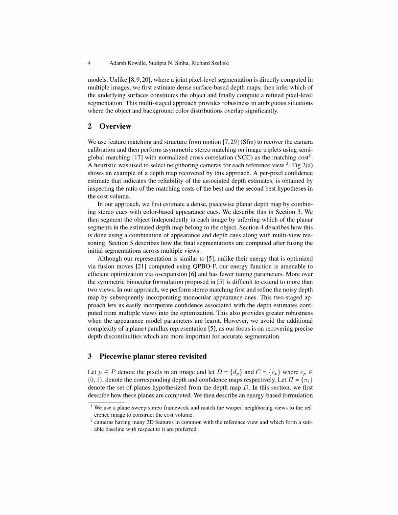
Fig. 3: (a) One of the initial depth maps from the BICYCLE sequence computed using [17].(b) The piecewise planar depth map obtained when only geometric cues are used. This is similarto [28]. (c) The depth map computed by our approach. Using appearance cues, both thin structuresand complex occlusion boundaries are accurately recovered.

towards high contrast image edges. We quantize the image by assigning to each pixelp, the mean color xsp in its superpixel and define the pairwise term for pixels p and q asEpq(lp, lq) = β0 + β1 exp

(−γ|xsp − xsq|2

)where lp 6= lq

3.

Learning the Parameters. In the first iteration, we minimize the energy defined inEquation 2 without the appearance-based unary terms by setting λG to 0. In subsequentiterations, λG is set to 100 and the appearance term is evaluated using GMM param-eters learnt from the labeling obtained from the previous iteration. To learn the GMMparameters for a plane, we consider the pixels assigned to it in the current labeling andconsider the distribution of confidence for these pixels. The t-th percentile of this dis-tribution is used to threshold and select confident pixels for training the GMMs. Weset t to 50. The GMM parameters are estimated using the EM algorithm after modelselection is used to determine the optimal number of mixture components. We allow amaximum of ten components and use the MDL (Rissanen) criterion [24] to select thevalue of K that maximizes the regularized posterior of all the nl pixels used to train theGMMs 4.

Unlike interactive segmentation [19,25,30] where training data is user-provided andalmost always reliable, the parameter learning step in our algorithm needs to be robustto noisy training samples, which arise due to errors in stereo matching. Usually, pixelswith inaccurate depths have low confidence when compared to accurate depth pixels.However there are exceptions – the confidence could be relatively high at specular sur-faces, or at occlusion boundaries with textureless occluded surfaces, even though thesepixels may have inaccurate depth estimates. Pixels on weakly textured surfaces, on theother hand, have low confidence even though their depth may be accurate [17].

We also use the confidence cp to weight the geometric term in the energy func-tion 2. This makes our approach robust to errors in stereo matching, which occur incases just described. As confidence estimates are usually low at textureless regions anddepth discontinuities, in both these cases the appearance term dominates the geometricterm. This enforces smoothness in homogeneous regions but also allows intricate oc-clusion boundaries to be recovered. Fig 3 shows an accurate depth map recovered for achallenging object with thin structures and holes.

3 Here, β0 = 1.0, β1 = 50.0, γ = 0.01 and x ∈ (0, 255).4 MDL criterion:

(−log(p(x|Al)) +

dim2log(nl)

), here dim = 3


4 Surface segmentation

Given a labeling L of pixels to planes, we now show how to infer which of the planarsegments belong to the object. We compute a binary labeling Fr over regions in L,using labels 0 and 1 for background and object respectively. We first reparameterize thelabeling L to obtain a new labeling L′ where each connected 2D segment has a uniquelabel. These regions are denoted as R = {ri}. We analyze all pairs of segments (ri, rj)and link them if their corresponding polygon in 3D are coplanar and satisfy a necessaryvisibility condition. To do this, we sort the pairs in decreasing order of the degree ofcoplanarity of their corresponding polygons and test them in a greedy fashion until allpairs within a threshold have been considered.

The visibility condition is as follows – by linking two coplanar polygons in 3D,a larger polygon is implicitly generated. If any part of this polygon occludes a planarsegment in the original depth map, it violates visibility and the regions are not linked.However, if the polygon is completely occluded by other segments, the regions can belinked. We implement this visibility check using an approach similar to [5], where itwas used to infer 3D connectivity of disconnected 2D segments. Linking disconnectedcoplanar regions lets us reason about them based on the visibility of their common 3Dplane in the multiple calibrated images. Finally, we have a new pixel to region labelingL′ and a many-to-one mapping from regions in L′ to a recomputed set of planes.

We now compute the region labeling Fr using energy minimization on two similarbinary pairwise MRFs defined on a graph over the regions r ∈ R with edges connectingadjacent regions denoted as NR. We compute labelings F ar and F gr by minimizing thetwo energy functions. 5

E(F ar ) =∑r∈R

EOr (fr) +∑

(r,t)∈NR

Eart(fr, ft) (4)

E(F gr ) =∑r∈R

EOr (fr) +∑

(r,t)∈NR

Egrt(fr, ft) (5)

The unary term EOr (fr) in both energy functions are identical. However, the pairwiseterms Eart (fr, ft) and Egrt (fr, ft) both of which favor label agreement, are differentand based on the compatibility of regions in terms of appearance and depth respectively.These energy functions can be efficiently minimized using an s-t mincut algorithm. Ingeneral, the two solutions F ar and F gr could be different. In the final segmentation Fr,a region is labeled as object if it is labeled object in either of the solutions. Otherwise itis labeled as background.

Multiview objectness unary term (EO). Using the camera calibration and piecewiseplanar depth induced by L′, we warp image pixels into the other views. If a pixelprojects within every other image, we say that it has high objectness. Since the ob-ject is assumed to be visible in every image, pixels with low objectness are likely to bebackground. Pixels with high objectness could either be object pixels or lie on back-ground surfaces that are within the field of view of every camera. Thus we measure the

5 Later in this section, we explain why we choose two energy functions instead of a single unifiedone.


objectness of a region r as the fraction of its pixels φr that have high objectness. Theterm is defined as EOr (0) = (1 + exp(−(φr − µ0)/σ0))

−1 and EOr (1) = 1 − EOr (0)where µ0 = 0.9, σ0 = 0.02. We force a region to take the foreground or backgroundlabel if φr > 0.99 or φr < .8 respectively, using hard constraints.

Appearance-based compatibility term (Eart). This term measures the dissimilarity ofthe color histograms of regions r and t. For this, we compute the KL-divergence be-tween their GMMs denoted as ρrt = DKL(Ar||At), where Ar and At are the GMMparameters, using the method proposed in [16]. The term is defined as Eart(fr, ft) =η1 exp(−µ1 min(ρrt, ρtr)) when fr 6= ft. When two dissimilar regions take differentlabels, there is a lower penalty than when the two regions are similar.

Depth-based compatibility term (Egrt). This term measures for two adjacent regionsin L′, how close their corresponding polygons are in 3D by computing the mean relativedepth discontinuity for pixels along the label boundary. Thus, for regions r and t, wefind a set B of pairs of adjacent pixels (pi, qi) that lie across the corresponding regionboundaries in L′. Denoting the depth of pixel p as dp, we define term as Egrt(fr, ft) =η2 exp(−µ2∆rt) where,

∆rt =1

|B|

|B|∑i=1

|dpi − dqi |/min(dpi , dqi)

We set parameters, η1 = 5.0, µ1 = 0.1, η2 = 5.0 and µ2 = 10.0.

Discussion. An alternative to our approach would have been to include both the pair-wise terms in a single energy function. However, this would require setting appropriateweights for the two terms, which is difficult in general. Occasionally, when the objectis camouflaged against the background, the appearance cue can be less reliable than thedepth cue, whereas when the depths along the region boundaries are approximate, thedepth cues can be less reliable. To avoid this interplay between the two pairwise termsin ambiguous cases, we chose to solve two energy functions as described and combinetheir results later. As the pairwise MRFs are small, there is negligible overhead in do-ing this. In practice, we often find the two segmentation F ar and F gr to be identical. Ingeneral, our approach has a slight bias towards over-segmenting the object, but this isrobustly handled in the final stage of our algorithm, described below.

5 Multi-view segmentation

The final stage in our approach exploits multi-view constraints to refine all the segmen-tations, which is similar to enforcing silhouette consistency in multiple views [9, 20].The binary labeling {Fr} of regions computed in the previous stage, induces a binarysegmentations of pixels. We denote this initial labeling as F i and the final labeling as Fand use a subscript j to indicate the j-th image in the sequence of N images, whenevernecessary. To compute F , we perform energy minimization on a pairwise binary MRFdefined on a 4-connected pixel grid (similar to the first stage of the algorithm describedin Section 3). Here we minimize the following energy function,

E(F ) =∑p∈P

EOp (fp) +∑p∈P

EAp (fp) +∑

(p,q)∈N

Epq(fp, fq) (6)


The unary terms EOp (fp) and EAp (fp) measure the cost of assigning pixel p to labelfp ∈ {0, 1} and the pairwise term Epq(lp, lq) penalizes label disagreement and has thesame definition as the pairwise term in Equation 2. We use the s-t mincut algorithm toexactly minimize the energy function.

Multi-view Objectness unary term (EO). This term measures the objectness of apixel, a term that was defined in Section 4. Unlike earlier, where the whole image wasconsidered to conservatively estimate a pixel’s objectness, we now use the availablesegmentations {F i}. For robustness, we compute a confidence-weighted estimate intwo passes, where the first pass computes a per-pixel weight reflecting the confidencein the pixel’s objectness. For each foreground pixel p in F ik, we warp it into every otherimage using the depth estimate computed in the first stage, and compute a fractionwp ∈[0, 1], indicating how often the warped pixels lies in the foreground in all the images.This is done by using the semi-dense depthmap recovered in Section 3.1, projecting the3D point onto all the views and computing the fraction of the views in which the pointlies within the foreground. For background pixels p in F ik, we set wp = 0.

In the second pass, we warp every pixel p in the j-th image into every other imageand set its objectness zp to the mean of the set of numbers {wq}, where q denotes thewarped pixel in the j-th image and wq its confidence computed in the first pass. We de-fine yp = (1+exp(−(zp − µ1)/σ1))

−1 where µ1 = 0.25, σ1 = 0.1. and define the unaryterm for the pixel in terms of yp for the binary labels as follows: EOp (1) = − log yp,and EOp (0) = − log(1− yp).

Appearance unary term (EA). We threshold the objectness estimates to select pix-els that we are confident about being in the set of foreground and background pix-els respectively 6. Appearance models based on GMMs of colors are now trained forthe foreground and background set, using model selection to determine the appropriatenumber of mixture components. The implementation details are similar to the first stage(Section 3.2). The penalty EAp is set to the negative log likelihood under the foregroundand background appearance models (see Equation 3 for details). Fig 4 shows an exam-ple demonstrating the advantages of multi-view reasoning in our method. We draw thereader’s attention to the two rear carriage wheels in this example, which get accuratelysegmented during the final stage.

6 Results

Datasets. We tested our algorithm on eight datasets and perform ground-truth evalua-tion for six datasets, which are summarized in Table 1. These datasets pose several chal-lenges for existing approaches as the object and background color distributions overlapsignificantly in many cases. Also in some images, the object contours are very faint dueto low image contrast. Illumination changes across images, diffused inter-reflectionsbetween object and backgrounds in many cases weakens the discriminability of the ap-pearance cues. The objects in these sequences contain thin structures and have complex

6 Concretely, we select pixels with yp > 0.7 and yp < 0.3 to serve as the selected foregroundand background pixels.


(a) (b) (c) (d)

Fig. 4: (a) One of the images in the CARRIAGE sequence. (b) The corresponding multi-viewobjectness measure. Foreground segmentations (c) before and (d) after the final multi-view con-sensus step. Notice how the the initial coarse segmentations are refined and the missing wheeland gaps between the wheels are recovered. In our formulation, the stone next to the rear carriagewheel gets segmented as part of the object.

topologies. The presence of textureless surfaces, strong specularities and reflections insome cases poses additional challenges for an automatic segmentation approach.

Evaluation. To evaluate our method, we used Grabcut [25] to segment the objectsin every image and treated these results as ground truth. Obtaining the ground truth in-teractively using Grabcut [25] on our sequences was an extremely tedious process. Forinstance, accurately segmenting the car, where glass windows reflect the background,the carriage and bicycle wheels where the background is seen through holes in the ob-ject, took up to 3 minutes on a single image and multiple user interactions. We evaluatedour method using the popular intersection over union metric [20], which is computedas the ratio of the size of the set intersection to that of the set union of the computed andground truth segmentation. The accuracy of our method across all datasets on averagewas 99.1 ± 0.8%. To evaluate the accuracy more strictly, we mark boundaries in thesegmentation and compute the unsigned distance transform with respect to these. Thisdistance map is thresholded to obtain a band of pixels around the boundary over whichthe accuracy is recomputed. Table 1 shows the accuracy for various thresholds. Witha threshold of 10 pixels, the average accuracy of our method was 90.9 ± 5.6%. Fig 5shows a few examples of segmentations and corresponding depth maps recovered byour method. More detailed results are presented on our website 7.

Comparisons. Fig 6 reports a quantitative comparison of our method with a stateof the art unsupervised cosegmentation approach [32]. Our method is consistently moreaccurate on all four sequences used in the comparison. The assumption in [32], that thebackground appearance changes across images more quickly than the foreground ap-pearance often causes the background to be misclassified as foreground on many of ourexamples. Our method is also significantly more flexible than existing automatic multi-view segmentation methods [8, 9] which rely on the fixation condition to learn the ob-ject’s appearance model. However, this may be difficult or even impossible for objectswith complex topologies such as the BICYCLE as the background is consistently seenthrough the object. In other cases, where the foreground contains multicolored objectssuch as in the CHAIR1 sequence, a single fixation point is unlikely to provide sufficientrepresentative samples for learning a color model for the complete foreground object.In comparison, our approach makes no assumptions about the shape or appearance ofthe object of interest.

7 http://chenlab.ece.cornell.edu/projects/MultiviewObjectCoseg


Fig. 5: [ COLUMNS 1 – 5] Results on CHAIR1, CHAIR2, BICYCLE, BIKE and CAR sequencesrespectively. [Row 1-3] A sample image from each dataset is shown along with its piecewise-planar surface labeling and the corresponding depth-map computed by our method. [Row 4] Thefinal segmentations recovered by our method. Notice how thin structures and holes in objectswith complex topologies are accurately segmented (see columns 1–3). Our method accuratelydeals with camouflage where the object and background colors are similar (see columns 4 and 5),and is also robust to the presence of strong specularities and reflections (see column 5).

Name #Images Acc-2 Acc-5 Acc-10 Acc-Full

COUCH 9 87.5± 2.0 93.9± 1.2 96.4± 0.7 99.6± 0.1

TEDDY 15 69.0± 4.9 79.5± 5.3 86.9± 3.8 98.8± 0.4

BIKE 34 83.8± 3.8 89.8± 4.1 92.7± 3.9 99.4± 0.4

CHAIR1 17 88.0± 4.6 91.4± 3.9 93.9± 3.1 99.2± 0.4

CHAIR2 45 90.5± 1.7 94.0± 0.8 95.8± 0.6 99.5± 0.1

CAR 45 74.8± 3.3 80.8± 2.9 84.2± 2.9 98.0± 0.7

Table 1: The percentage of correctly labeled pixels (mean±std. dev.) in the segmentations com-puted by our method is listed for six datasets (see text for details).

Although our piecewise planar stereo method is closely related to [5], their methodcannot ensure that the foreground will be segmented as a single object. This makes itdifficult to compare the methods quantitatively. A C++ implementation of our approachruns in under 2 minutes on a PC with an Intel 3GHz Xeon processor and 4GB RAMon a single 640 × 480 resolution image. Approximately one minute is spent on thepiecewise planar depth map estimation step. In comparison, the method proposed in [5]takes 20 mins. on a single Middlebury image pair.

7 Conclusions

In this work, we have proposed an unsupervised algorithm to obtain the joint multiviewforeground segmentation. We have developed a novel approach that combines multi-view cues and appearance cues in a hierarchical reasoning framework to extract out the


Vicente’11 [32] Grabcut [25] Ours PMVS [14]

Name Vicente’11 [32] PMVS [14] Ours

BIKEAcc-10 68.1± 6.7 61.0± 3.9 90.0± 4.9

Acc-Full 88.9± 6.3 96.0± 1.8 99.1± 0.7

BICYCLEAcc-10 56.5± 3.1 56.2± 1.8 89.8± 3.8

Acc-Full 81.7± 8.9 89.1± 3.9 98.0± 0.5

CHAIR1Acc-10 73.3± 4.8 72.7± 2.1 93.9± 3.1

Acc-Full 86.9± 7.8 96.6± 0.4 99.2± 0.4

CARAcc-10 74.4± 5.3 59.6± 4.3 83.2± 1.1

Acc-Full 91.8± 4.3 91.2± 5.5 97.9± 0.6

Fig. 6: COMPARISONS: Two out of 61 images from the BICYCLE sequence are shown. [Column1] shows results from Vicente et. al. [32] in the red overlay. [Column 2] shows results from Grab-cut [25] with exhaustive user input. [Column 3] shows our results. [Column 4] shows resultsgenerated from a 3D reconstuction (PMVS [14]) with manual segmentation. Our segmentationsare accurate on thin structures such as the handle-bars and wheel rims and visually comparableto Grabcut [25] on this example. The interactive segmentation took 4 minutes during which theuser had to provide about 80 strokes to obtain a perfect result. [BOTTOMLEFT] The foregroundand background strokes drawn by the user are shown in blue and yellow respectively. [BOTTOM-RIGHT] Quantitative accuracy of our results compared to [14, 32].

foreground object across the multiple views. As we show via quantitative and qualita-tive results, our algorithm accurately handles a wide variety of objects that pose chal-lenges due to specular surfaces, diverse and overlapping color distributions, complexocclusions, and thin structures.

References

1. X. Bai, J. Wang, D. Simons, and G. Sapiro. Video SnapCut: robust video object cutout usinglocalized classifiers. In SIGGRAPH, 2009.

2. D. Batra, A. Kowdle, D. Parikh, J. Luo, and T. Chen. iCoseg: Interactive co-segmentationwith intelligent scribble guidance. CVPR, 2010.

3. S. Birchfield and C. Tomasi. Multiway cut for stereo and motion with slanted surfaces. InICCV, 1999.

4. M. Bleyer, C. Rother, and P. Kohli. Surface stereo with soft segmentation. CVPR, 2010.5. M. Bleyer, C. Rother, P. Kohli, D. Scharstein, and S. Sinha. Object stereo - joint stereo

matching and object segmentation. CVPR, 2011.6. Y. Boykov, O. Veksler, and R. Zabih. Efficient approximate energy minimization via graph

cuts. PAMI, 20(12):1222–1239, 2001.


7. M. Brown and D. G. Lowe. Unsupervised 3d object recognition and reconstruction in un-ordered datasets. In 3DIM, pages 56–63, 2005.

8. N. Campbell, G. Vogiatzis, C. Hernandez, and R. Cipolla. Automatic 3d object segmentationin multiple views using volumetric graph-cuts. Image and Vision Computing, 28:14–25,2010.

9. N. Campbell, G. Vogiatzis, C. Hernandez, and R. Cipolla. Automatic object segmentationfrom calibrated images. In CVMP, 2011.

10. D. Cohen-Steiner, P. Alliez, and M. Desbrun. Variational shape approximation. ACM Trans.Graph., 23:905–914, 2004.

11. A. Criminisi, G. Cross, A. Blake, and V. Kolmogorov. Bilayer segmentation of live video.In CVPR, pages 53–60, 2006.

12. A. Criminisi, T. Sharp, and A. Blake. Geos: Geodesic image segmentation. In ECCV, 2008.13. Y. Furukawa, B. Curless, S. Seitz, and R. Szeliski. Manhattan-world stereo. In CVPR, 2009.14. Y. Furukawa, B. Curless, S. M. Seitz, and R. Szeliski. Towards internet-scale multi-view

stereo. In CVPR, 2010.15. D. Gallup, J.-M. Frahm, and M. Pollefeys. Piecewise planar and non-planar stereo for urban

scene reconstruction. In CVPR, 2010.16. J. Goldberger, S. Gordon, and H. Greenspan. An efficient image similarity measure based

on approximations of kl-divergence between two gaussian mixtures. In ICCV, 2003.17. H. Hirschmuller. Stereo processing by semiglobal matching and mutual information. PAMI,

30(2):328–341, 2008.18. D. S. Hochbaum and V. Singh. An efficient algorithm for co-segmentation. In ICCV, 2009.19. A. Kowdle, D. Batra, W. Chen, and T. Chen. iModel: Interactive co-segmentation for object

of interest 3d modeling. In ECCV - RMLE Workshop, 2010.20. W. Lee, W. Wontack, and E. Boyer. Silhouette segmentation in multiple views. PAMI, 2010.21. V. S. Lempitsky, C. Rother, S. Roth, and A. Blake. Fusion moves for markov random field

optimization. PAMI., 32(8):1392–1405, 2010.22. L. Mukherjee, V. Singh, and C. Dyer. Half-integrality based algorithms for cosegmentation

of images. In CVPR, 2009.23. L. Quan, J. Wang, P. Tan, and L. Yuan. Image-based modeling by joint segmentation. IJCV,

75:135–150, October 2007.24. J. Rissanen. Modeling by shortest data description. Automatica, 14:465–471, 1978.25. C. Rother, V. Kolmogorov, and A. Blake. Grabcut: interactive foreground extraction using

iterated graph cuts. In SIGGRAPH, 2004.26. C. Rother, T. Minka, A. Blake, and V. Kolmogorov. Cosegmentation of image pairs by

histogram matching - incorporating a global constraint into mrfs. In CVPR, 2006.27. I. Simon and S. M. Seitz. Scene segmentation using the wisdom of crowds. In ECCV, pages

541–553, 2008.28. S. Sinha, D. Steedly, and R. Szeliski. Piecewise planar stereo for image-based rendering. In

ICCV, 2009.29. N. Snavely, S. Seitz, and R. Szeliski. Photo tourism: Exploring photo collections in 3d. In

SIGGRAPH, 2006.30. M. Sormann, C. Zach, and K. Karner. Graph cut based multiple view segmentation for 3d

reconstruction. 3DPVT, 0:1085–1092, 2006.31. H. Tao, H. Sawhney, and R. Kumar. A global matching framework for stereo computation.

In ICCV, pages 532–539, 2001.32. S. Vicente, C. Rother, and V. Kolmogorov. Object cosegmentation. In CVPR, 2011.33. J. W. Weingarten, G. Gruener, and R. Siegwart. Probabilistic plane fitting in 3d and an

application to robotic mapping. In ICRA, pages 927–932, 2004.34. J. Xiao, J. Chen, D.-Y. Yeung, and L. Quan. Structuring visual words in 3d for arbitrary-view

object localization. In ECCV, 2008.35. J. Xiao, J. Wang, P. Tan, and L. Quan. Joint affinity propagation for multiple view segmen-

tation. In ICCV, 2007.

multiple view object cosegmentation using … view object cosegmentation using appearance and stereo...

Documents