Multiple scaling behavior and nonlinear traits in musicscoresAlfredo Gonzalez-Espinoza*,1,2,3, Hernan Larralde2, Gustavo Martınez-Mekler2,3,5,and Markus Muller*,3,4,5

1 Instituto de Investigacion en Ciencias Basicas y Aplicadas, UAEM, Morelos, Mexico2 Instituto de Ciencias Fısicas, UNAM, Morelos, Mexico3 Centro de Ciencias de la Complejidad, UNAM, CDMX, Mexico4 Centro de Investigacion en Ciencias, UAEM, Morelos, Mexico

5 Centro Internacional de Ciencias, A.C., Morelos, Mexico

*jage@icf.unam.mx, *muellerm@uaem.mx

Keywords: Detrended Fluctuation Analysis, Time Series, Music Scores, Nonlinear Correlations.

Abstract

We present a statistical analysis of music scores from different composers using detrended fluctuation analysis. Wefind different fluctuation profiles that correspond to distinct auto-correlation structures of the musical pieces. Further,we reveal evidence for the presence of nonlinear auto-correlations by estimating the detrended fluctuation analysis ofthe magnitude series, a result validated by a corresponding study of appropriate surrogate data. The amount and thecharacter of nonlinear correlations vary from one composer to another. Finally, we performed a simple experiment inorder to evaluate the pleasantness of the musical surrogate pieces in comparison with the original music and find thatnonlinear correlations could play an important role in the aesthetic perception of a musical piece.

Introduction

Music is a complex construct that involves cultural factors, acoustic features, interpretation techniques and audienceperception. Its ample range of properties make it a fascinating study subject from many different viewpoints, inaddition to its relevance in our everyday life. The study of Music from the perspective of statistical physics has beenof great interest during the last decades. One of the pioneering works in this context, using techniques from statisticalphysics, was published by Voss and Clarke [1]. They estimated the spectral density of intensity fluctuations and founda power law behavior close to 1/f noise. This result inspired many researchers to study the statistical properties ofmusic, ranging from the identification of temporal patterns or power laws, to the development of algorithms for musiccomposition [2–11]. Amongst these, are the identification of mayor and minor tonalities in Bach’s Well-TemperedClavier by means of a statistical parametrization [6], the role of correlated noise in the humanization of melodiesproduced by computers [8], and the analysis of the interplay between voices in the three-part inventions by Bach [10].

Power laws or scaling laws are manifestations of self-similarity in the world around us [12–15]. In music, the 1/fβ

spectra with β = 1 has been interpreted in [9,16] as a trade off between predictability and surprise, if β tends to lowervalues (zero is the case of white noise), the temporal sequence of notes is highly uncorrelated and sounds unpleasant.On the other hand, if β becomes too large the music becomes monotonous. Scaling behaviors, in particular 1/fβ

with 1 < β < 2 have been found frequently in music [2, 4, 5, 9–11]. However, few of the studies have focused onmusic scores [4,10,16], and to the best of our knowledge, none presents a detailed analysis of the scaling behaviorin the pitch fluctuations of pieces from different composers. It should be noted that unique scaling laws in musicalpieces are not always present, indeed, scaling exponents may vary on different time scales [2, 4]. This raises thequestion of which auto-correlation structures, apart from a constant scaling, are actually present in musical pieces,

1/20

arX

iv:1

708.

0898

2v5

[ph

ysic

s.so

c-ph

] 8

Nov

201

7

20 40 60 80 100 120 140#Note

40

50

60

70

80

MID

I pitc

h

Bach's crab canon from BWV 1079

Figure 1. The famous crab canon from the Musical Offering by Bach. The Y axis indicates the value of the notewithin the range 0-127, the x axis corresponds to the number of notes written in the unit defined by the note of theoriginal piece with shortest duration. The two different voices of the piece are indicated in the blue and red lines.

and what, if any, is the relation between characteristic correlation profiles and composition rules, music periodor particular composers. Furthermore, there may be other interrelations in musical pieces that are not capturedby the auto-correlation function that could be relevant for the aesthetic appreciation of music. We refer to theseinterrelations as nonlinear auto-correlations. To our knowledge this is the first time that nonlinear considerationshave been addressed in the statistical analysis of music.

In this work we focus on music scores, interpreting them as multi-variate time series to which we applied differenttype of fluctuation analysis. We provide a consistent interpretation of the fluctuation profiles, which are markedlydifferent for different composers. The structure of the musical pieces is partly reflected in their auto-correlation,which gives guidelines or elements to characterize the composition process. We try to detect and first classify differentauto-correlation profiles of musical pieces stemming from different periods of time. This characterization couldcontribute to the development of composition models. Furthermore, we search for the presence of nonlinear features,which may be present on different time scales. Finally, we present a first attempt to test whether such nonlinearfeatures play a role in the aesthetic perception of music.

Materials and Methods

Construction of the time series

We consider music scores as a sequence of integer numbers, each of them labeling a different note. The numberswere extracted from midi files obtained from different web databases [17, 18]. We processed the midi files usingmidicsv [19], a free software that converts midi into csv (comma-separated values) files. Taking the note with thesmallest duration as the time unit, a time series can be generated as shown in Figure 1. An improved understandingof such representation can be attained from Figures 2 and 3. In 3 the first eight measures of the piece shown in 2 aretranslated in units of the shortest note (in the figure we subdivided each note into eighth notes, which represent theshortest duration of the original piece and serves as the time unit in this case). The time series is multi-variate andthe number of variables depends on the number of instruments or voices of the piece.

2/20

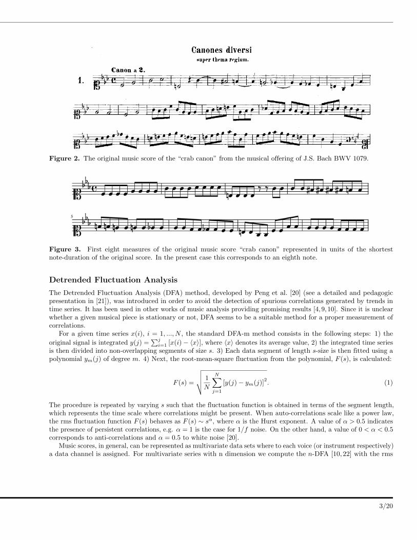
Figure 2. The original music score of the “crab canon” from the musical offering of J.S. Bach BWV 1079.

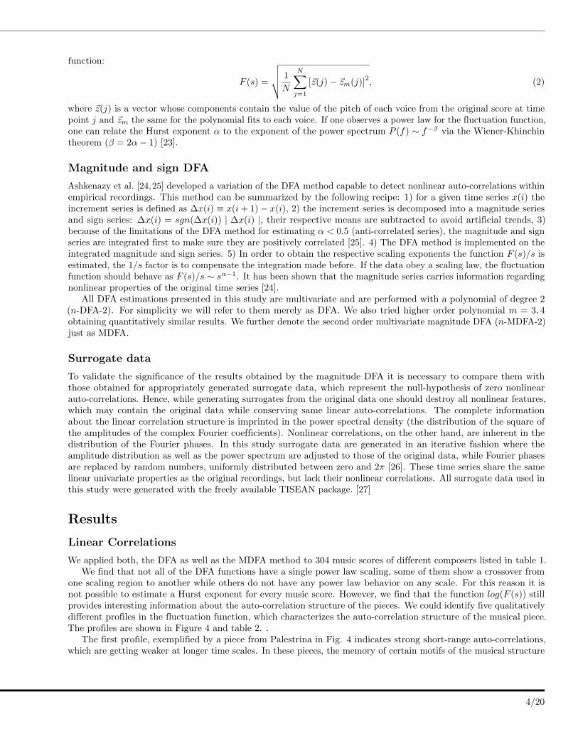
Figure 3. First eight measures of the original music score “crab canon” represented in units of the shortestnote-duration of the original score. In the present case this corresponds to an eighth note.

Detrended Fluctuation Analysis

The Detrended Fluctuation Analysis (DFA) method, developed by Peng et al. [20] (see a detailed and pedagogicpresentation in [21]), was introduced in order to avoid the detection of spurious correlations generated by trends intime series. It has been used in other works of music analysis providing promising results [4, 9, 10]. Since it is unclearwhether a given musical piece is stationary or not, DFA seems to be a suitable method for a proper measurement ofcorrelations.

For a given time series x(i), i = 1, ..., N , the standard DFA-m method consists in the following steps: 1) the

original signal is integrated y(j) =∑ji=1 [x(i)− 〈x〉], where 〈x〉 denotes its average value, 2) the integrated time series

is then divided into non-overlapping segments of size s. 3) Each data segment of length s-size is then fitted using apolynomial ym(j) of degree m. 4) Next, the root-mean-square fluctuation from the polynomial, F (s), is calculated:

F (s) =

√√√√ 1

N

N∑j=1

[y(j)− ym(j)]2. (1)

The procedure is repeated by varying s such that the fluctuation function is obtained in terms of the segment length,which represents the time scale where correlations might be present. When auto-correlations scale like a power law,the rms fluctuation function F (s) behaves as F (s) ∼ sα, where α is the Hurst exponent. A value of α > 0.5 indicatesthe presence of persistent correlations, e.g. α = 1 is the case for 1/f noise. On the other hand, a value of 0 < α < 0.5corresponds to anti-correlations and α = 0.5 to white noise [20].

Music scores, in general, can be represented as multivariate data sets where to each voice (or instrument respectively)a data channel is assigned. For multivariate series with n dimension we compute the n-DFA [10,22] with the rms

3/20

function:

F (s) =

√√√√ 1

N

N∑j=1

[~z(j)− ~zm(j)]2, (2)

where ~z(j) is a vector whose components contain the value of the pitch of each voice from the original score at timepoint j and ~zm the same for the polynomial fits to each voice. If one observes a power law for the fluctuation function,one can relate the Hurst exponent α to the exponent of the power spectrum P (f) ∼ f−β via the Wiener-Khinchintheorem (β = 2α− 1) [23].

Magnitude and sign DFA

Ashkenazy et al. [24,25] developed a variation of the DFA method capable to detect nonlinear auto-correlations withinempirical recordings. This method can be summarized by the following recipe: 1) for a given time series x(i) theincrement series is defined as ∆x(i) ≡ x(i+ 1)− x(i), 2) the increment series is decomposed into a magnitude seriesand sign series: ∆x(i) = sgn(∆x(i)) | ∆x(i) |, their respective means are subtracted to avoid artificial trends, 3)because of the limitations of the DFA method for estimating α < 0.5 (anti-correlated series), the magnitude and signseries are integrated first to make sure they are positively correlated [25]. 4) The DFA method is implemented on theintegrated magnitude and sign series. 5) In order to obtain the respective scaling exponents the function F (s)/s isestimated, the 1/s factor is to compensate the integration made before. If the data obey a scaling law, the fluctuationfunction should behave as F (s)/s ∼ sα−1. It has been shown that the magnitude series carries information regardingnonlinear properties of the original time series [24].

All DFA estimations presented in this study are multivariate and are performed with a polynomial of degree 2(n-DFA-2). For simplicity we will refer to them merely as DFA. We also tried higher order polynomial m = 3, 4obtaining quantitatively similar results. We further denote the second order multivariate magnitude DFA (n-MDFA-2)just as MDFA.

Surrogate data

To validate the significance of the results obtained by the magnitude DFA it is necessary to compare them withthose obtained for appropriately generated surrogate data, which represent the null-hypothesis of zero nonlinearauto-correlations. Hence, while generating surrogates from the original data one should destroy all nonlinear features,which may contain the original data while conserving same linear auto-correlations. The complete informationabout the linear correlation structure is imprinted in the power spectral density (the distribution of the square ofthe amplitudes of the complex Fourier coefficients). Nonlinear correlations, on the other hand, are inherent in thedistribution of the Fourier phases. In this study surrogate data are generated in an iterative fashion where theamplitude distribution as well as the power spectrum are adjusted to those of the original data, while Fourier phasesare replaced by random numbers, uniformly distributed between zero and 2π [26]. These time series share the samelinear univariate properties as the original recordings, but lack their nonlinear correlations. All surrogate data used inthis study were generated with the freely available TISEAN package. [27]

Results

Linear Correlations

We applied both, the DFA as well as the MDFA method to 304 music scores of different composers listed in table 1.We find that not all of the DFA functions have a single power law scaling, some of them show a crossover from

one scaling region to another while others do not have any power law behavior on any scale. For this reason it isnot possible to estimate a Hurst exponent for every music score. However, we find that the function log(F (s)) stillprovides interesting information about the auto-correlation structure of the pieces. We could identify five qualitativelydifferent profiles in the fluctuation function, which characterizes the auto-correlation structure of the musical piece.The profiles are shown in Figure 4 and table 2. .

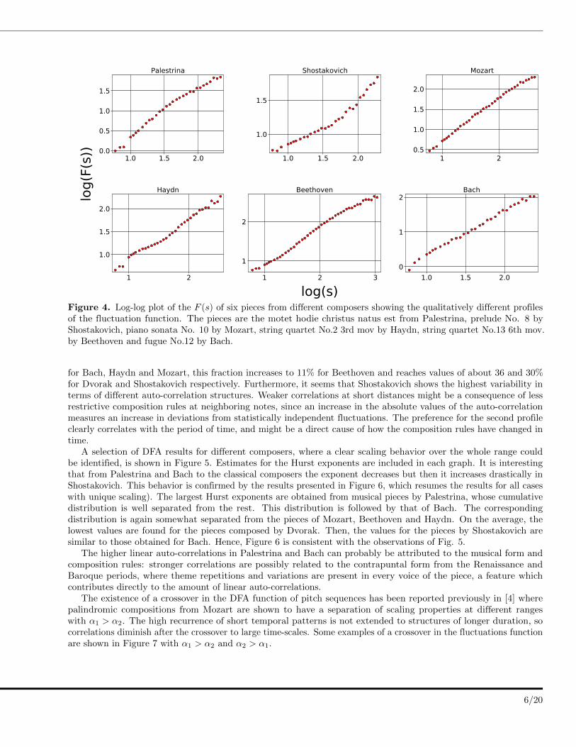
The first profile, exemplified by a piece from Palestrina in Fig. 4 indicates strong short-range auto-correlations,which are getting weaker at longer time scales. In these pieces, the memory of certain motifs of the musical structure

4/20

Composer birth-death number of piecesPalestrina 1525-1594 21Bach 1685-1750 63Haydn 1732-1809 48Mozart 1756-1791 36Beethoven 1780-1827 63Dvorak 1841-1904 25Shostakovich 1906-1975 48

Table 1. Name of the composer, year of birth and death and number of the pieces analyzed. The list is in chronologicalorder from top to bottom.

Profile

Palestrina

Bach

Haydn

Mozart

Beethoven

Shostakovich

15 0 5 10

30 2 24 7 0

25 2 14 2 5

22 1 11 0 2

17 7 35 3 1

15 14 17 2 0

Composer

Dvorak 4 8 10 2 1

Table 2. Classification by fluctuation profiles of the pieces analyzed in this study. The first row shows the fivedifferent profiles we could identify. Numbers indicate the amount of scores of each composer with a given profile. Theclassification has been done by careful eye inspection of the scaling plots.

of small durations gets lost on longer time scales such that self-similarity is diluted and irregularity increases. Suchtype of crossovers have already been identified in [4].

Counter-intuitively, the second profile shows opposite characteristics: Correlations at large time scales are strongerthan those at short times scales (see the example of Shostakovich in Fig. 4). These large time correlations, which aresimilar in magnitude to those of the first profile, are indicative of the recurrence of long patterns. However, in thiscase short sequences of notes are more irregular.

A third profile consists of a constant scaling behavior over the whole range of box sizes s. An example is providedby a piece of Mozart in Fig. 4. The two remaining profiles correspond to different changes of curvature, illustrated byBeethoven and Bach in Fig. 4, showing a more irregular behavior, where stronger and less strong auto-correlatedtime scales alternate.

Table 2 summarizes the number of opus of a given composer, which could be assigned to one of the profiles of thefluctuation function. Although Table 2 is not necessarily conclusive, it provides some trends, which allow to roughlydistinguish composers. For instance, Profile 1 (stronger short range than long-range correlations) and Profile 3 (aclear scaling over the whole range) are the preferred correlation profiles for all composers except Dvorak, for whomwe identified an important percentage of pieces with fluctuation profile 2 in comparison of profile 1. In particularPalestrina shows a clear preference for profile 1. On the other hand, pieces by Shostakovich, Dvorak and to someextent also those by Beethoven, are, relative to the composers selected in this study, most frequently assigned toprofile 2. There, stronger auto-correlations act on longer time scales. Furthermore, while Beethoven inclines to profile3, Mozart and Haydn show a preference for profile 1. Finally, Bach has highest scoring at profile 4 and Haydn forprofile 5. At all, Haydn, Beethoven and Dvorak show scoring for all five profiles.

We find it interesting that the number of pieces corresponding to the second profile apparently increases the lateris the musical period of the composer. While the percentage of such profile detected in this study is about 3 to 4%

5/20

log(s)

log(F(s))

Figure 4. Log-log plot of the F (s) of six pieces from different composers showing the qualitatively different profilesof the fluctuation function. The pieces are the motet hodie christus natus est from Palestrina, prelude No. 8 byShostakovich, piano sonata No. 10 by Mozart, string quartet No.2 3rd mov by Haydn, string quartet No.13 6th mov.by Beethoven and fugue No.12 by Bach.

for Bach, Haydn and Mozart, this fraction increases to 11% for Beethoven and reaches values of about 36 and 30%for Dvorak and Shostakovich respectively. Furthermore, it seems that Shostakovich shows the highest variability interms of different auto-correlation structures. Weaker correlations at short distances might be a consequence of lessrestrictive composition rules at neighboring notes, since an increase in the absolute values of the auto-correlationmeasures an increase in deviations from statistically independent fluctuations. The preference for the second profileclearly correlates with the period of time, and might be a direct cause of how the composition rules have changed intime.

A selection of DFA results for different composers, where a clear scaling behavior over the whole range couldbe identified, is shown in Figure 5. Estimates for the Hurst exponents are included in each graph. It is interestingthat from Palestrina and Bach to the classical composers the exponent decreases but then it increases drastically inShostakovich. This behavior is confirmed by the results presented in Figure 6, which resumes the results for all caseswith unique scaling). The largest Hurst exponents are obtained from musical pieces by Palestrina, whose cumulativedistribution is well separated from the rest. This distribution is followed by that of Bach. The correspondingdistribution is again somewhat separated from the pieces of Mozart, Beethoven and Haydn. On the average, thelowest values are found for the pieces composed by Dvorak. Then, the values for the pieces by Shostakovich aresimilar to those obtained for Bach. Hence, Figure 6 is consistent with the observations of Fig. 5.

The higher linear auto-correlations in Palestrina and Bach can probably be attributed to the musical form andcomposition rules: stronger correlations are possibly related to the contrapuntal form from the Renaissance andBaroque periods, where theme repetitions and variations are present in every voice of the piece, a feature whichcontributes directly to the amount of linear auto-correlations.

The existence of a crossover in the DFA function of pitch sequences has been reported previously in [4] wherepalindromic compositions from Mozart are shown to have a separation of scaling properties at different rangeswith α1 > α2. The high recurrence of short temporal patterns is not extended to structures of longer duration, socorrelations diminish after the crossover to large time-scales. Some examples of a crossover in the fluctuations functionare shown in Figure 7 with α1 > α2 and α2 > α1.

6/20

log(s)

log

(F(s

))α = 1.43 α = 1.40

α = 1.06

α = 1.16 α = 0.96 α = 1.33

Figure 5. DFA functions from different composers that exhibit a clear scaling behavior over the whole range suchthat a Hurst exponent can be assigned. The pieces are: fugue No.4 of the WTK by Bach, motet oh bone jesu byPalestrina, string quartet OP. 76 4th mov. by Haydn, string quartet No.16 3rd mov. by Mozart, string quartet No.155th mov. by Beethoven and fugue No.16 by Shostakovich.

By simple eye revision, the presence of two different time scales can be appreciated in the patterns of the originaltime series shown in Figures 8 and 9. Within the range of 1-20 notes in Bach’s sonata we can observe many quitesimilar patterns of pitch fluctuations, this similarity weakens on larger time scales. This explains the larger slopelog(F (s)) at the first time scale while it decreases from α1 = 1.4 to α2 = 0.9 for distance s > 20, which is indicativeof weaker correlations.

The opposite happens in the case of the Fugue from Shostakovich (Figure 9), where the correlations on shortertime scales are considerably weak, they change from α1 = 0.6 to α2 = 0.9 at about s < 32. At short time scales thepitch fluctuations are more irregular and close to white noise (α = 0.5), hence melodic patterns are more difficult topredict. However, on longer time scales motives of note sequences are (almost) repeated, which explains the presenceof stronger long-range correlations.

Figure 10 shows a plot α1 vs α2 taking into account all musical pieces of the different composers which show acrossover in their fluctuation function. The center of each ellipse is defined by the mean of each (α1, α2)-distribution,while the axis reflect their respective standard deviations. Note that the interval of variation of α1 is considerablylarger than the one for α2, this is an indication that changes in long-range correlations are more restricted than inshort-range ones. Thus, overall structure of the musical forms are more preserved amongst the various composersthan are the motifs. The Figure shows that it is not possible to distinguish the composers just by the adjustedα-values due to the fact that the dispersion in the distributions causes several ellipses to overlap to a large extent.However, at least some trends can be identified. For instance, opus from Dvorak tend to have the lowest α1 andlargest α2 values, viz. long-range correlations are stronger than short-range. The opposite is true for Palestrina,Bach, Haydn and Mozart. In their pieces short-range correlations dominate. The marked eccentricity in the ellipse ofMozart manifests higher dispersion in short-range correlations. This is not the case for Bach, where eccentricity isalmost absent. In Palestrina’s ellipse though there is some eccentricity, the change in orientation of the axis shows acorrelation contribution opposite to Mozart. The most equilibrated in terms of short- and long-range auto-correlationsare opus’ composed by Beethoven and Shostakovich whose ellipse are closer to the main diagonal of the graph. Thedispersion in the ellipses indicates the most varied composers are Dvorak and Shostakovich, while the least variedis Palestrina, a result which again might be directly related to changes of the composer rules. Recall the findings

7/20

α

P(α)

Figure 6. Cumulative distribution functions for the α exponent extracted for different composers. α-exponentsentering in this statistics are exclusively estimated for those cases where a unique scaling has been observed over thewhole range of box sizes.

log(s)

log(F(s))

α1=1.41

α2=0.91

α1=1.42 α1=1.24

α1=1.52 α1=1.25

α1=0.65

α2=0.92 α2=0.66

α2=0.83α2=0.86 α2=0.90

Figure 7. Fluctuation function of six pieces derived from different composers: 1st mov of the Sonata soprıl SoggettoReale by Bach, motet hodie christus natus est from Palestrina, string quartet No.1 5th mov. by Haydn, string quartetNo.18 4th mov. by Mozart, string quartet No.2 2nd mov. by Beethoven and fugue No.23 by Shostakovich. For fiveof the log(F (s)) function the two exponents obey α1 > α2 but in Shostakovich’s fugue Hurst exponents are relateddifferently: α2 > α1.

8/20

Figure 8. Extract from the first movement of the Sonata sopr’il Soggetto Reale, horizontal square brackets of equalcolor indicate where similar patterns are, different colors are for different patterns, the ticks on the x axis are thecrossover size sc =20, they to identify contributions in the range where the correlations with slope α1 are.

Figure 9. Extract from the music score of Shostakovich’s 23 fugue, horizontal square brackets of equal color indicatewhere similar patterns are, in this case the ticks on the x axis are of the crossover size sc = 32.

9/20

α1

α2

Figure 10. α2 vs α1 plot for the 162 pieces that exhibit a crossover in their fluctuations function. Each of theellipses represents a composer. They are centered at the mean values of their α1 and α2 exponents. The axis arefixed by the respective standard deviation of Hurst exponents.

listed in Table 2, where Dvorak and Shostakovich showed a more frequent preference for the second auto-correlationprofile with α2 > α1. In general, we found for these two composers a more uniform distribution among the differentcorrelation profiles, which also indicates a higher variability of composing schemes. For the other composers α2 < α1

is more recurrent. The appearance of two scaling exponents can be attributed to the presence of motifs as well aslonger sections in the structure of the musical piece. Stronger short-range correlations (α2 < α1) are evidence ofsimilar motifs repeated throughout the piece; while weaker short-range correlations (α2 > α1) arise when the pieceincorporates more varied short time patterns. In both cases, the structure given by the sections of the musical pieceis reflected at long time scales. In a unique scaling case (α2 = α1), the musical patterns are preserved at all timescales, from motifs to phrases and sections.

Even though there is evidence of correlations in their fluctuations we are unable to extend these analysis to theremaining profiles (4 and 5) due to their scarcity. To verify that these results are not a particularity of the multivariateapplication of the DFA method, we also applied DFA individually to each voice finding quantitatively similar resultsfor the various log(F (s)) functions (Fig. S2). As mentioned before, scaling information can also be obtained from theseries power spectra. In the supplementary material (Fig. S3), as an example, we show cases of three different profiles.The localization of the crossover is consistent with the DFA calculations, however in the latter they are better definedand more precise. The expected scaling relations among the exponents are corroborated

Nonlinearity

Music, as well as language, are prototypes of so called “complex systems”, which are frequently governed by nonlinearinterrelations (although that is not a necessary requirement). Nonlinearity of a time series has been related tomulti-fractality [26] and previous studies have already reported multi-fractal properties of music [5, 28, 29]. In view ofthese results, we search for nonlinear auto-correlations in the present work. To this end we generate surrogate dataand apply Detrended Fluctuation Analysis to the “magnitude series” [24] of both original and surrogate time series.

10/20

log(s)

log(F(s))

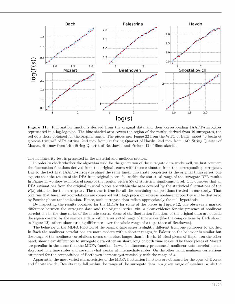
Figure 11. Fluctuation functions derived from the original data and their corresponding IAAFT-surrogatesrepresented in a log-log-plot. The blue shaded area covers the region of the results derived from 19 surrogates, thered dots those obtained for the original music. The pieces are: Fugue 22 from the WTC of Bach, motet ”o beata etgloriosa trinitas” of Palestrina, 2nd mov from 1st String Quartet of Haydn, 2nd mov from 15th String Quartet ofMozart, 4th mov from 14th String Quartet of Beethoven and Prelude 12 of Shostakovich.

The nonlinearity test is presented in the material and methods section.In order to check whether the algorithm used for the generation of the surrogate data works well, we first compare

the fluctuation functions derived from the original scores with those estimated from the corresponding surrogates.Due to the fact that IAAFT-surrogates share the same linear univariate properties as the original times series, oneexpects that the results of the DFA from original pieces fall within the statistical range of the surrogate DFA results.In Figure 11 we show examples of some of the results, with a 5% of statistical significance level. One observes that allDFA estimations from the original musical pieces are within the area covered by the statistical fluctuations of theF (s) obtained for the surrogates. The same is true for all the remaining compositions treated in our study. Thatconfirms that linear auto-correlations are conserved with high precision whereas nonlinear properties will be destroyedby Fourier phase randomization. Hence, such surrogate data reflect appropriately the null-hypothesis.

By inspecting the results obtained for the MDFA for some of the pieces in Figure 12, one observes a markeddifference between the surrogate data and the original series, viz. a clear evidence for the presence of nonlinearcorrelations in the time series of the music scores. Some of the fluctuation functions of the original data are outsidethe region covered by the surrogate data within a restricted range of time scales (like the compositions by Bach shownin Figure 12), others show striking differences over the whole range of s (e.g. those of Beethoven).

The behavior of the MDFA function of the original time series is slightly different from one composer to another.In Bach the nonlinear correlations are more evident within shorter ranges, in Palestrina the behavior is similar butthe range of the nonlinear correlations seems somewhat longer than in Bach. Musical pieces of Haydn, on the otherhand, show clear differences to surrogate data either on short, long or both time scales. The three pieces of Mozartare peculiar in the sense that the MDFA function shows simultaneously pronounced nonlinear auto-correlations onshort and long time scales and are somewhat weaker at intermediate scales. On the other hand, nonlinear correlationsestimated for the compositions of Beethoven increase systematically with the range of s.

Apparently, the most varied characteristics of the MDFA fluctuation functions are obtained for the opus’ of Dvorakand Shostakovich. Results may fall within the range of the surrogate data in a given range of s-values, while the

11/20

fluctuation functions lie far outside of this region on other scales. They may differ simultaneously for large and shorttime scales, while being similar for intermediate values of s. For other pieces, the opposite behavior can be found,where solely on intermediate time scales clear differences to the surrogate results appear. In other cases the behaviormay be qualitatively similar to compositions of Beethoven (increasing amount of nonlinear correlations with the timescale) or those of Bach (clear differences to the surrogates can only be found on short time scales).

12/20

log(F(s)/s)

Bach

Palestrina

Haydn

Mozart

Beethoven

Shostakovich

Dvorak

log(s)

Figure 12. MDFA functions for three different pieces of each composer. The blue shaded area represents the regioncovered by the fluctuation functions of the 19 surrogates while the red dots correspond to the results obtained forthe original time series. The pieces are listed in the supplementary material. Dots outside the shaded regions areindicative of the presence of nonlinear correlations.

13/20

Discussion

In the present study we performed a statistical analysis of musical scores from several periods, focused on the behaviorof correlations, looking into their range, scaling properties and also a means for the detection of nonlinearity. To thisend we resorted to Detrended Fluctuation Analysis, which circumvents the question of whether musical pieces arestationary, which is important in short time series such as these. Furthermore, that provides a uniform approachfor the detection and characterization of lineal as well as nonlinear auto-correlations. With the implementation of amodified DFA for intervals and comparison with surrogate data, we tested the presence of nonlinear traits.

Regarding the power laws

We found that though a considerable fraction of all compositions treated in this study (38%) show a clear powerlaw scaling over the whole range of possible time scales, the dominant profile (53%) shows a crossover between twoscaling regimes. This observation is corroborated by the determination of DFA exponents. The fact that the strengthof short-range auto-correlations might be different from that of long-range dependencies provides an indicator forqualitatively different composition structures. In our study, it turned out that usually short-range correlation aremore pronounced than auto-correlations in long time scales. Although, via the estimation of Hurst exponents we haveso far been unable to determine a certain musical period or the style of a particular composer, some trends can beidentified and for some composers specific traits have been uncovered. For example, in Shostakovich we find thatpieces with stronger long-range correlations are almost as frequent as those with stronger short-range correlations,this feature seems to reflect a particular style of this composer. The above is even more pronounced for Dvorak,although with poorer statistics, here we found that pieces with stronger long-range correlations are twice as frequentas those with dominant short-range auto-correlations. Another clear example comes from Palestrina for whom thefinding of a marked dominance of short-range correlations over long ones appears to be a hallmark of his style. Ingeneral, the location of the distribution of the musical pieces within the (α1;α2)-plane is revealing.

Another interesting aspect in the context of a possible classifier is the presence of nonlinear auto-correlations. Thefluctuation analysis of the magnitude series, together with an adequately designed surrogate test, provides an efficienttool for the detection and characterization of nonlinear dependencies within musical scores. Here we find stronghints of peculiar, composer specific, nonlinear features. Magnitude as well as the temporal range where significantdifferences with the results obtained from surrogate data may serve as indicators for specific temporal structures of amusical piece.

However, these findings are not conclusive due the poor statistics, but we strongly believe that linear as well asnonlinear auto-correlations structures are prominent candidates for characterizing certain epochs or, equivalently,particular composer styles. Further analysis in this direction is surely required.

The pleasantness of the nonlinear correlations

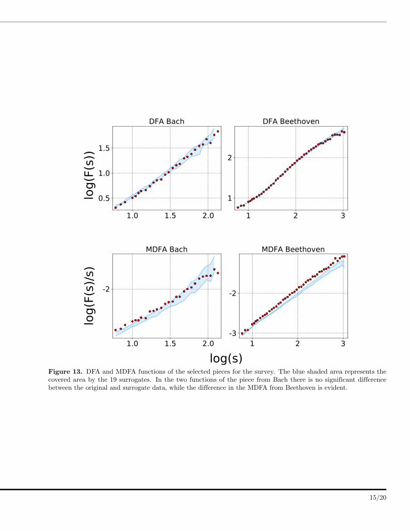
Since the work of Voss and Clarke [1] on music audio voltage there have been numerous studies that refer to 1/fcorrelated noise in music as the most pleasant to human ear [4,9,10,30]. In this case the relation between fluctuationsat different scales is preserved with a power law behavior. There is a scale invariance in the power spectrum which bythe Wiener-Khinchin relation is also manifest in the linear auto-correlation. On the other hand it has been arguedby A. Schoenberg that in order to optimize aesthetic appreciation of a musical piece, a certain equilibrium betweenregular time structures and variation should be encountered [31]. Though scaling in linear auto-correlations mayplay a crucial role in this regard, regularity is not necessarily produced by self-similarity of different fragments of amusical piece. Nonlinear auto-interrelationships might generate less obvious, but possibly not less fascinating regularfeatures. However, to the best of our knowledge, there are so far no studies mentioning nonlinear correlations in music.We designed an experiment in order to probe the aesthetic quality of the presence of nonlinear auto-correlations incompositions. To this end we selected two different pieces and their corresponding surrogates (see Fig. 13). TheMDFA of one composition created by Bach evidences only a weak contribution of nonlinear correlations, which arefurthermore exclusively present on short time scales. The other opus from Beethoven, shows nonlinear features on allscales, whose magnitude is growing with s. The selected pieces are the prelude no. 6 of the well tempered clavierfrom Bach and the finale of the 13th string quartet from Beethoven.

14/20

log(s)

log(F(s))

log(F(s)/s)

Figure 13. DFA and MDFA functions of the selected pieces for the survey. The blue shaded area represents thecovered area by the 19 surrogates. In the two functions of the piece from Bach there is no significant differencebetween the original and surrogate data, while the difference in the MDFA from Beethoven is evident.

15/20

Frequency

Pleasantness ScoreFigure 14. Distributions of the pleasantness score obtained from the survey, blue bars represent the distribution forthe original piece, red bars represent the distribution of the surrogate piece.

We constructed MIDI sonifications of the two original pieces and their respective surrogates and conducted asurvey for a quantitative evaluation of the aesthetic quality of each. In total 1,281 persons were consulted on howpleasant they perceived each of them in a scale from 1 (highly unpleasant) to 10 (most pleasant), for more details onthe experiment see the supplementary material. The results are summarized in Figure 14.

In both cases, the evaluation of the original pieces turned out to be quite positive, with an accumulation ofthe scores between 8 and 10. However, the evaluation of the surrogate pieces was much more surprising. Here thesurrogate composition by Bach received significantly less low qualifications (1 and 2) and simultaneously more higherscores (in particular a score of 8) than in Beethoven.

The lack of nonlinear correlations in the original piece of Bach means that most of the regular structure isincorporated in the power spectrum. Self-similar musical motives are preserved under the conservation of the powerspectrum. Therefore, also the surrogates maintain somehow the equilibrium between order and disorder of the originalpiece and encounter a benevolent evaluation.

The situation is different in the case of Beethoven’s 13th string quartet. According to our results this compositioncontains an important amount of nonlinear correlations, which are destroyed in the surrogate music. Under theseconditions the power spectra alone no longer assures the fine coordination between ordered repetition of motives andstructural variability. Nonlinear correlations play now a major role and the musical piece differs much more from thenoisy character of the surrogates. This last statement is not only true for the obvious case of Beethoven’s 13th stringquartet, where nonlinear features are quite pronounced; even for the prelude No.6 of the well tempered clavier fromBach, where nonlinear correlations are seemingly present in a subtle manner, they play nevertheless an importantrole for the aesthetic appreciation. Also in this case we measured a striking difference between the evaluation of theoriginal piece and the surrogate replica. Hence, we may conclude that in general, aesthetic perception in musicalcompositions depends importantly on their nonlinear auto-correlation time structures.

16/20

About algorithmic composition

One of the main interests for understanding musical structures is the development algorithmic composition. Markovmodels, neural networks and generative grammars have been proven to be successful in generating note sequenceswith musical meaning at short time scales [32–34]. However, the research in the development of new models withshort and long correlations is still of interest in statistical physics [35–37]. The characterization of linear as wellas nonlinear auto-correlations and the time scales where they are present could lead to more realistic models. Theinclusion of nonlinear scaling behavior by means of stochastic models could be helpful in the development of newtechniques in algorithmic composition.

Conclusions

We have presented an analysis of music scores using Detrended Fluctuation Analysis. We were able to identifydifferent profiles in the fluctuation functions, which could be used for further classification of musical pieces.

We found that not all the pieces have simple scale invariance in their fluctuations function, indeed the presenceof a crossover between two different scaling regimes is more frequent. This evidences that pieces have differentstatistical behaviors within different ranges i.e. different correlations at different time scales. By looking into thecorrelation profiles we uncovered traits in the composition styles of some of the musicians. We exemplified the relationof structural modules with correlations at different time scales in two pieces. We also uncovered clear tendencies incomposers and temporal evolution of compositions related with the cumulative distributions of the α exponents (inthe case of single scaling) and with the mean and dispersion of the α1 and α2 exponents (in the crossover cases).

We further applied the MDFA method to the music scores and found evidence of the presence of nonlinearcorrelations. Similar to the linear DFA approach, different profiles for F (s)/s were encountered. We were unable, sofar, to establish a relationship between the scaling profiles obtained by DFA and those of MDFA. We constructedsurrogate pieces preserving the linear correlations of the original compositions and undertook a survey in order toevaluate the pleasantness of the surrogates. We found that nonlinear correlations could play an important role in theaesthetic appreciation of the musical pieces.

One of the aims of this paper was to contribute to establish criteria for the classification of musical compositions,some progress was achieved in this respect with the analysis of the different profiles identified in the DFA function.Additionally, our study provides elements and tools for the analysis of specific pieces. We believe this approach to theanalysis of music scores, which unravels characteristics of composers, musical forms and periods, has the potential ofcontributing to the understanding of further issues such as musical evolution, composition and perception.

Ethics

The authors were not required to complete an ethical assessment prior to conducting this research.

Permission to carry out fieldwork

No permissions were required prior to conducting this research.

Data Availability

The data and the code used in this work, as well as the supplementary material are deposited at Dryad [38]:https://doi.org/10.5061/dryad.6737v

Autors’ contribution

A.G-E. and M.M. designed the experiments for the data analysis, A.G-E. collected the data, implemented the codefor constructing the time series and computing the DFA and MDFA. A.G-E and M.M. designed and implemented the

17/20

survey. All authors analyzed and interpreted the results. All authors contributed and reviewed the manuscript. Allauthors gave final approval for publication.

Competing Interests

The authors declare no competing interests.

Funding

A. G-E. acknowledges CONACyT for the financial support under the scholarship No. 258226 during his graduatedstudies, M.M. acknowledges financial support from CONACyT Mexico, Proj. No. CB-156667, H.L. acknowledgesfinancial support from PAPIIT, UNAM, Proj. No. IN110016.

Acknowledgements

We thank Daniel Alejandro Priego-Espinosa for the fruitful feedback in the group discussions.

References

1. Richard F Voss. ”1/f noise” in music: Music from 1/f noise. The Journal of the Acoustical Society of America,63(1):258, 1978.

2. Heather D Jennings, Plamen Ch Ivanov, Allan de M. Martins, P.C da Silva, and G.M Viswanathan. Variancefluctuations in nonstationary time series: a comparative study of music genres. Physica A: Statistical Mechanicsand its Applications, 336(3-4):585–594, may 2004.

3. Gungor Gunduz and Ufuk Gunduz. The mathematical analysis of the structure of some songs. Physica A:Statistical Mechanics and its Applications, 357(3-4):565–592, 2005.

4. Leonardo Dagdug, Jose Alvarez-Ramirez, Carlos Lopez, Rodolfo Moreno, and Enrique Hernandez-Lemus.Correlations in a Mozart’s music score (K-73x) with palindromic and upside-down structure. Physica A:Statistical Mechanics and its Applications, 383(2):570–584, 2007.

5. G R Jafari, P Pedram, and L Hedayatifar. Long-range correlation and multifractality in Bach’s Inventionspitches. Complexity, 2007(04):18, 2007.

6. M. Beltran del Rıo, G. Cocho, and G. G. Naumis. Universality in the tail of musical note rank distribution.Physica A: Statistical Mechanics and its Applications, 387(22):5552–5560, 2008.

7. Gustavo Martınez-Mekler, Roberto Alvarez Martınez, Manuel Beltran del Rıo, Ricardo Mansilla, PedroMiramontes, and Germinal Cocho. Universality of rank-ordering distributions in the arts and sciences. PLoSONE, 4(3), 2009.

8. Holger Hennig, Ragnar Fleischmann, Anneke Fredebohm, York Hagmayer, Jan Nagler, Annette Witt, Fabian J.Theis, and Theo Geisel. The nature and perception of fluctuations in human musical rhythms. PLoS ONE,6(10), 2011.

9. Daniel J Levitin, Parag Chordia, and Vinod Menon. Musical rhythm spectra from Bach to Joplin obey a 1/fpower law. Proceedings of the National Academy of Sciences, 109(10), 2012.

10. Luciano Telesca and Michele Lovallo. Analysis of temporal fluctuations in Bach’s sinfonias. Physica A: StatisticalMechanics and its Applications, 391(11):3247–3256, 2012.

18/20

11. Lu Liu, Jianrong Wei, Huishu Zhang, Jianhong Xin, and Jiping Huang. A Statistical Physics View of PitchFluctuations in the Classical Music from Bach to Chopin: Evidence for Scaling. PLoS ONE, 8(3):1–6, 2013.

12. Stuart Kauffman. At Home in the Universe: The search for laws of self-organization and complexity. OxfordUniversity Press, 1995.

13. Per Bak. How Nature Works: The Science of self-organized criticality. Springer, 1996.

14. Manfred Schroeder. Fractals, chaos, power laws: minutes from an infinite paradise. W. H. Freeman andCompany, 1991.

15. Geoffrey West. Scale. Penguin Press, New York, 2017.

16. Dan Wu, Keith M. Kendrick, Daniel J. Levitin, Chaoyi Li, and Dezhong Yao. Bach is the father of harmony:Revealed by a 1/f fluctuation analysis across musical genres. PLoS ONE, 10(11):1–17, 2015.

17. Petrucci music library. http://imslp.org/.

18. The largest classical music resource in .mid files. http://www.kunstderfuge.com/.

19. miditocsv software. http://www.fourmilab.ch/webtools/midicsv/.

20. C. K. Peng, S. V. Buldyrev, S. Havlin, M. Simons, H. E. Stanley, and A. L. Goldberger. Mosaic organization ofDNA nucleotides. Physical Review E, 49(2):1685–1689, 1994.

21. Detrended fluctuation analysis (dfa). https://www.physionet.org/tutorials/fmnc/node5.html.

22. Erika E. Rodrıguez, Enrique Hernandez-Lemus, Benjamın A. Itza-Ortiz, Ismael Jimenez, and Pablo Rudomın.Multichannel detrended fluctuation analysis reveals synchronized patterns of spontaneous spinal activity inanesthetized cats. PLoS ONE, 6(10), 2011.

23. Norbert Wiener. Generalized harmonic analysis. Acta Mathematica, 55(C):117–258, 1930.

24. Yosef Ashkenazy, Plamen Ch Ivanov, Shlomo Havlin, Chung K. Peng, Ary L. Goldberger, and H. EugeneStanley. Magnitude and sign correlations in heartbeat fluctuations. Physical Review Letters, 86(9):1900–1903,2001.

25. Yosef Ashkenazy, Shlomo Havlin, Plamen Ch Ivanov, Chung K. Peng, Verena Schulte-Frohlinde, and H. EugeneStanley. Magnitude and sign scaling in power-law correlated time series. Physica A: Statistical Mechanics andits Applications, 323:19–41, 2003.

26. Thomas Schreiber and Andreas Schmitz. Surrogate time series. Physica D: Nonlinear Phenomena, 142(3-4):346–382, 2000.

27. Nonlinear time series analysis. www.mpipks-dresden.mpg.de/ tisean/.

28. Zhi Yuan Su and Tzuyin Wu. Multifractal analyses of music sequences. Physica D: Nonlinear Phenomena,221(2):188–194, 2006.

29. Zhi Yuan Su and Tzuyin Wu. Music walk, fractal geometry in music. Physica A: Statistical Mechanics and itsApplications, 380(1-2):418–428, 2007.

30. Yu. L Klimontovich and J.-P Boon. Natural Flicker Noise (“1/f Noise”) in Music. Europhysics Letters (EPL),3(4):395–399, 1987.

31. Arnold Schoenberg. Theory of Harmony. London: Faber & Faber, 1978.

32. Xiao Fan Liu, Chi K. Tse, and Michael Small. Complex network structure of musical compositions: Algorithmicgeneration of appealing music. Physica A: Statistical Mechanics and its Applications, 389(1):126–132, 2010.

33. Eduardo R. Miranda. Composing Music with Computers. Focal PElsevier, 2002.

19/20

34. Gerhard Nierhaus. Algorithmic Composition: Paradigms of Automated Music Generation. Springer, 2009.

35. Jason Sakellariou, Francesca Tria, Vittorio Loreto, and Francois Pachet. Maximum entropy models capturemelodic styles. pages 1–25, 2016.

36. Jason Sakellariou, Francesca Tria, Vittorio Loreto, and Francois Pachet. Maximum Entropy Model for MelodicPatterns. Proceedings of the 32nd International Conference on Machine Learning, 37, 2015.

37. Gaetan Hadjeres and Francois Pachet. DeepBach: a Steerable Model for Bach chorales generation. pages 1–20,2016.

38. A Gonzalez-Espinoza, H Larralde, G Martınez-Mekler, and M Mueller. Data from: Multiple scaling behaviorand nonlinear traits in music scores.

20/20