multiple linear regression.pptx
DESCRIPTION
a report on multiple linear regressionTRANSCRIPT
IAPRI Quantitative Analysis Capacity Building Series
Multiple regression analysis & interpreting results
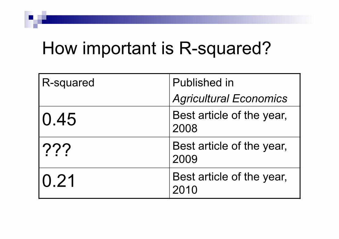
How important is R-squared?
R-squared Published in Agricultural Economics
0.45 Best article of the year, 2008
??? Best article of the year, 2009
0.21 Best article of the year, 2010
Session 3 Topics
n Multiple regression analysis ¨ What does it mean? ¨ Why is it important? ¨ How is it done and how are results interpreted? ¨ What are the hazards?
Multiple Regression Analysis n What does it mean?
¨ Multivariate analysis/statistics ¨ “Ceteris paribus” ¨ “All else equal” ¨ “Controlling for”
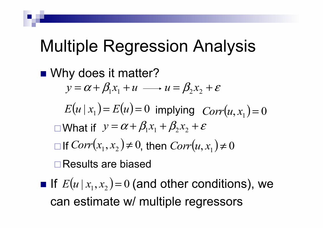
Multiple Regression Analysis n Why does it matter?
implying
¨ What if
¨ If , then
¨ Results are biased
n If (and other conditions), we can estimate w/ multiple regressors
uxy ++= 11βα
( ) ( ) 0| 1 == uExuE ( ) 0, 1 =xuCorr
εβ += 22xu
( ) 0, 21 ≠xxCorr ( ) 0, 1 ≠xuCorr
( ) 0,| 21 =xxuE
εββα +++= 2211 xxy
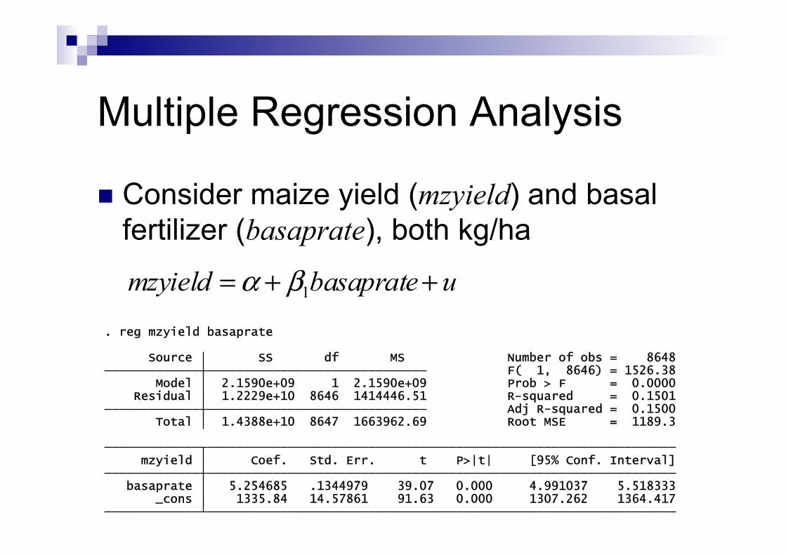
Multiple Regression Analysis
n Consider maize yield (mzyield) and basal fertilizer (basaprate), both kg/ha
_cons 1335.84 14.57861 91.63 0.000 1307.262 1364.417 basaprate 5.254685 .1344979 39.07 0.000 4.991037 5.518333 mzyield Coef. Std. Err. t P>|t| [95% Conf. Interval]
Total 1.4388e+10 8647 1663962.69 Root MSE = 1189.3 Adj R-squared = 0.1500 Residual 1.2229e+10 8646 1414446.51 R-squared = 0.1501 Model 2.1590e+09 1 2.1590e+09 Prob > F = 0.0000 F( 1, 8646) = 1526.38 Source SS df MS Number of obs = 8648
. reg mzyield basaprate
ubasapratemzyield ++= 1βα

Multiple Regression Analysis
n Top dressing (topaprate) determines yield and is correlated with basaprate, both kg/ha
_cons 1314.93 14.58701 90.14 0.000 1286.336 1343.524 topaprate 3.62044 .3157663 11.47 0.000 3.001463 4.239418 basaprate 1.897807 .321747 5.90 0.000 1.267106 2.528508 mzyield Coef. Std. Err. t P>|t| [95% Conf. Interval]
Total 1.4387e+10 8646 1664061.58 Root MSE = 1180.5 Adj R-squared = 0.1626 Residual 1.2046e+10 8644 1393535.34 R-squared = 0.1628 Model 2.3418e+09 2 1.1709e+09 Prob > F = 0.0000 F( 2, 8644) = 840.22 Source SS df MS Number of obs = 8647
. reg mzyield basaprate topaprate
εββα +++= topapratebasapratemzyield 21
Multiple Regression Analysis
n is the intercept n are slope parameters (usually)
uxxxy kk +++++= βββα ...2211
αβ

8
y
x 1 2 3
1β slope
intercept α
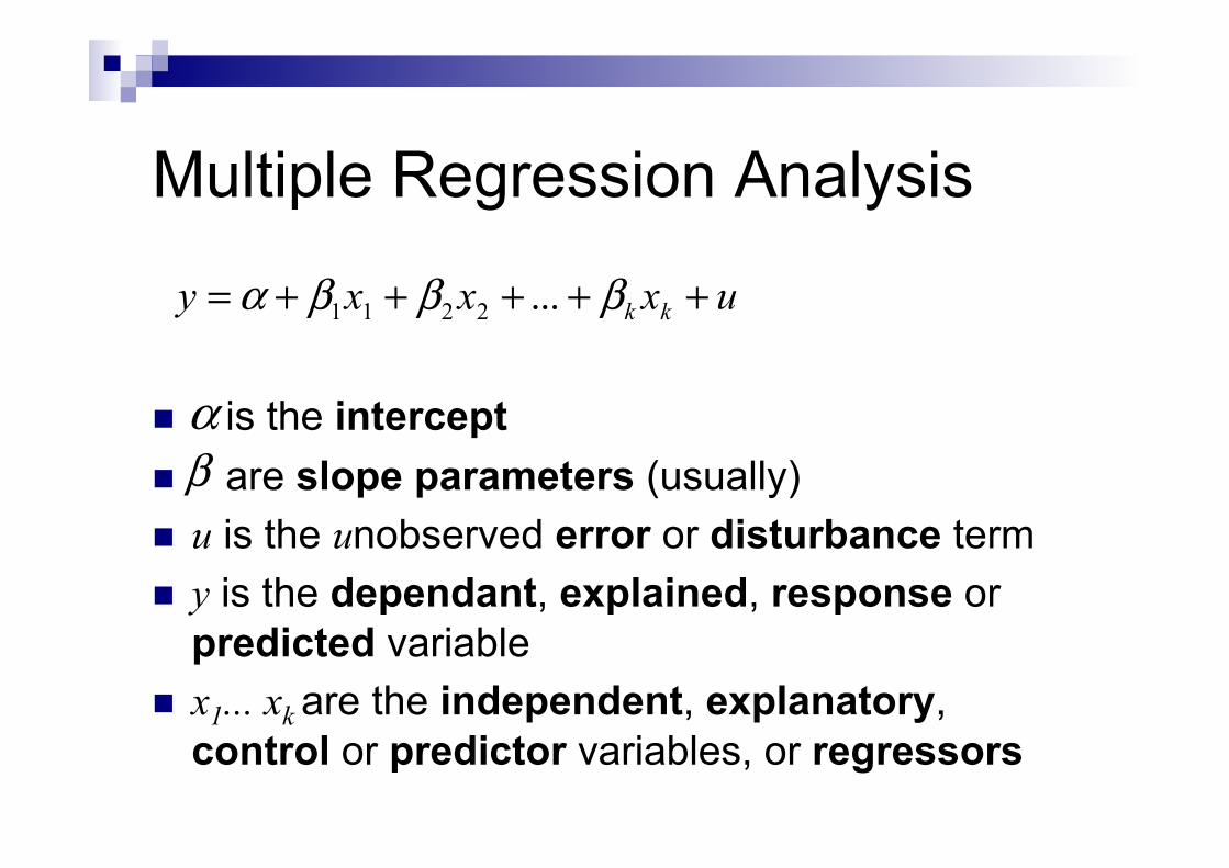
Multiple Regression Analysis
n is the intercept n are slope parameters (usually) n u is the unobserved error or disturbance term n y is the dependant, explained, response or
predicted variable n x1... xk are the independent, explanatory,
control or predictor variables, or regressors
uxxxy kk +++++= βββα ...2211
αβ
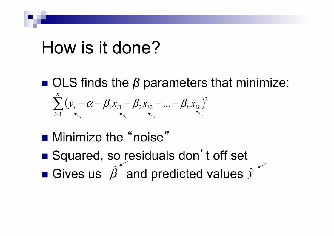
How is it done?
n OLS finds the β parameters that minimize: n Minimize the “noise” n Squared, so residuals don’t off set n Gives us and predicted values β
( )∑=
−−−−−n
iikkiii xxxy
1
22211 ... βββα
y
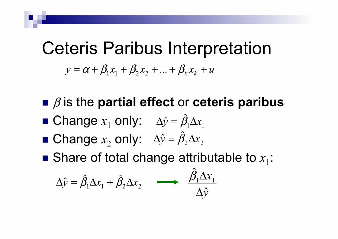
Ceteris Paribus Interpretation uxxxy kk +++++= βββα ...2211
n is the partial effect or ceteris paribus n Change x1 only: n Change x2 only: n Share of total change attributable to x1:
β
11ˆˆ xy Δ=Δ β
22ˆˆ xy Δ=Δ β
yxˆ
ˆ11
ΔΔβ
2211ˆˆˆ xxy Δ+Δ=Δ ββ
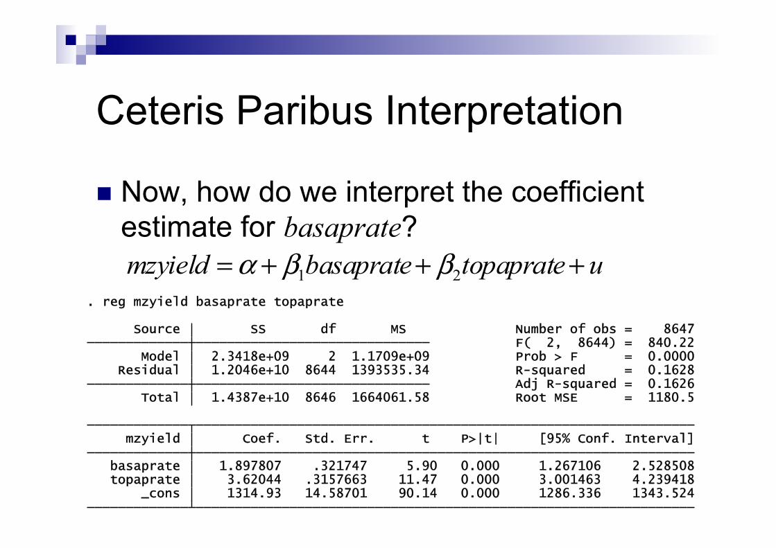
Ceteris Paribus Interpretation
n Now, how do we interpret the coefficient estimate for basaprate?
_cons 1314.93 14.58701 90.14 0.000 1286.336 1343.524 topaprate 3.62044 .3157663 11.47 0.000 3.001463 4.239418 basaprate 1.897807 .321747 5.90 0.000 1.267106 2.528508 mzyield Coef. Std. Err. t P>|t| [95% Conf. Interval]
Total 1.4387e+10 8646 1664061.58 Root MSE = 1180.5 Adj R-squared = 0.1626 Residual 1.2046e+10 8644 1393535.34 R-squared = 0.1628 Model 2.3418e+09 2 1.1709e+09 Prob > F = 0.0000 F( 2, 8644) = 840.22 Source SS df MS Number of obs = 8647
. reg mzyield basaprate topaprate
utopapratebasapratemzyield +++= 21 ββα

Ceteris Paribus Interpretation
n “According to these results, a one unit change in x1 will result in a unit change in y, all else equal.”
n “The ceteris paribus effect of a one unit change in x1 is a unit change in y.”
n Holding x2 constant, a one unit change in x1 results in a unit change in y.”
1β
1β
β

Key Assumptions
n Linear in parameters n Random sample n Zero conditional mean n No perfect collinearity (variation in data) n Homoskedastic errors
Key Assumptions
n Linear in parameters n Random sample n Zero conditional mean n No perfect collinearity (variation in data) n Homoskedastic errors

Perfect Collinearity
n Variable is a linear function of one or more others.
n No variation in one variable (collinear w/intercept)

Can’t estimate slope parameter if no variation in x
17 Source: Wooldridge (2002)
Perfect Collinearity
n Variable is a linear function of one or more others.
n No variation in one variable (collinear w/intercept)
n Perfect correlation between 2 binary variables
Other hazards
n Multi-collinearity n Including irrelevant variables n Omitting relevant variables
Multi-Collinearity
n Highly correlated variables n Variable is a nonlinear function of others n What’s the problem? n Efficiency losses n Schmidt thumb rule
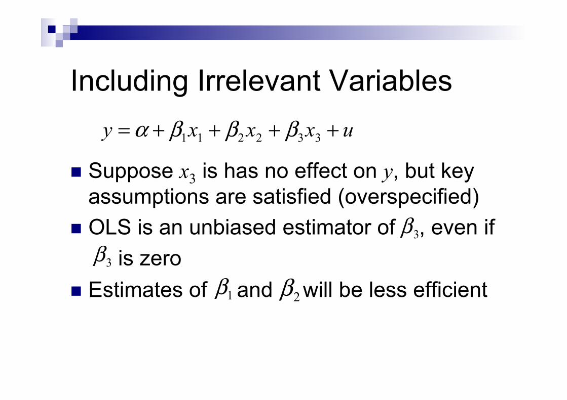
Including Irrelevant Variables
n Suppose x3 is has no effect on y, but key assumptions are satisfied (overspecified)
n OLS is an unbiased estimator of , even if is zero n Estimates of and will be less efficient
uxxxy ++++= 332211 βββα
3β3β
1β 2β
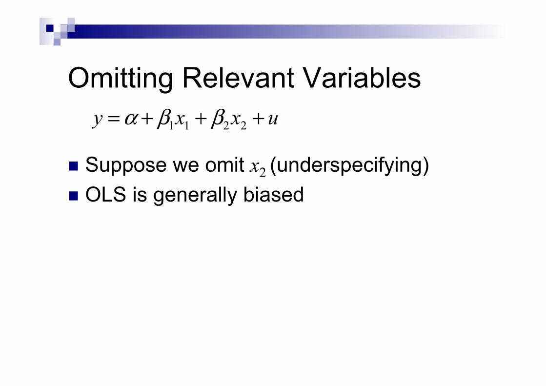
Omitting Relevant Variables
n Suppose we omit x2 (underspecifying) n OLS is generally biased
uxxy +++= 2211 ββα
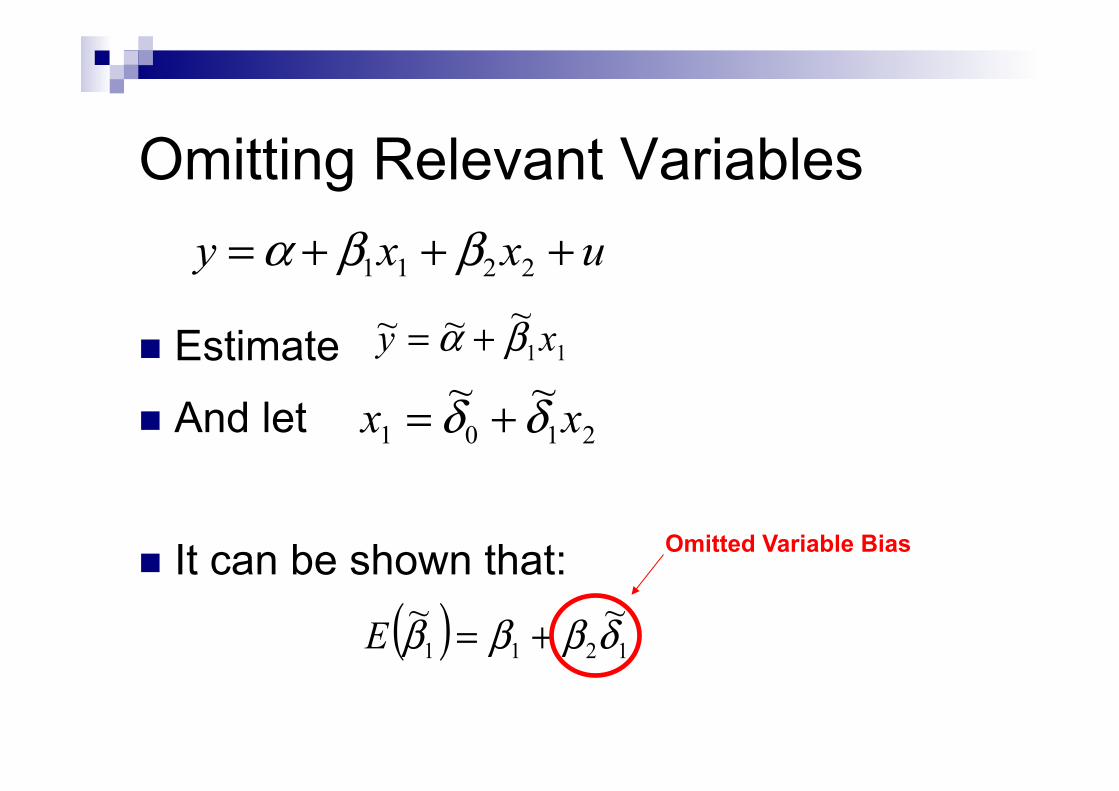
Omitting Relevant Variables
n Estimate
n And let
n It can be shown that:
11~~~ xy βα +=
uxxy +++= 2211 ββα
2101~~ xx δδ +=
( ) 1211~~ δβββ +=E
Omitted Variable Bias

Multiple Regression Analysis
Corr(x1,x2)>0 Corr(x1,x2)<0
Positive bias Negative bias
Negative bias Positive bias
Source: Wooldridge, 2002, page 92
02 >β
02 <β
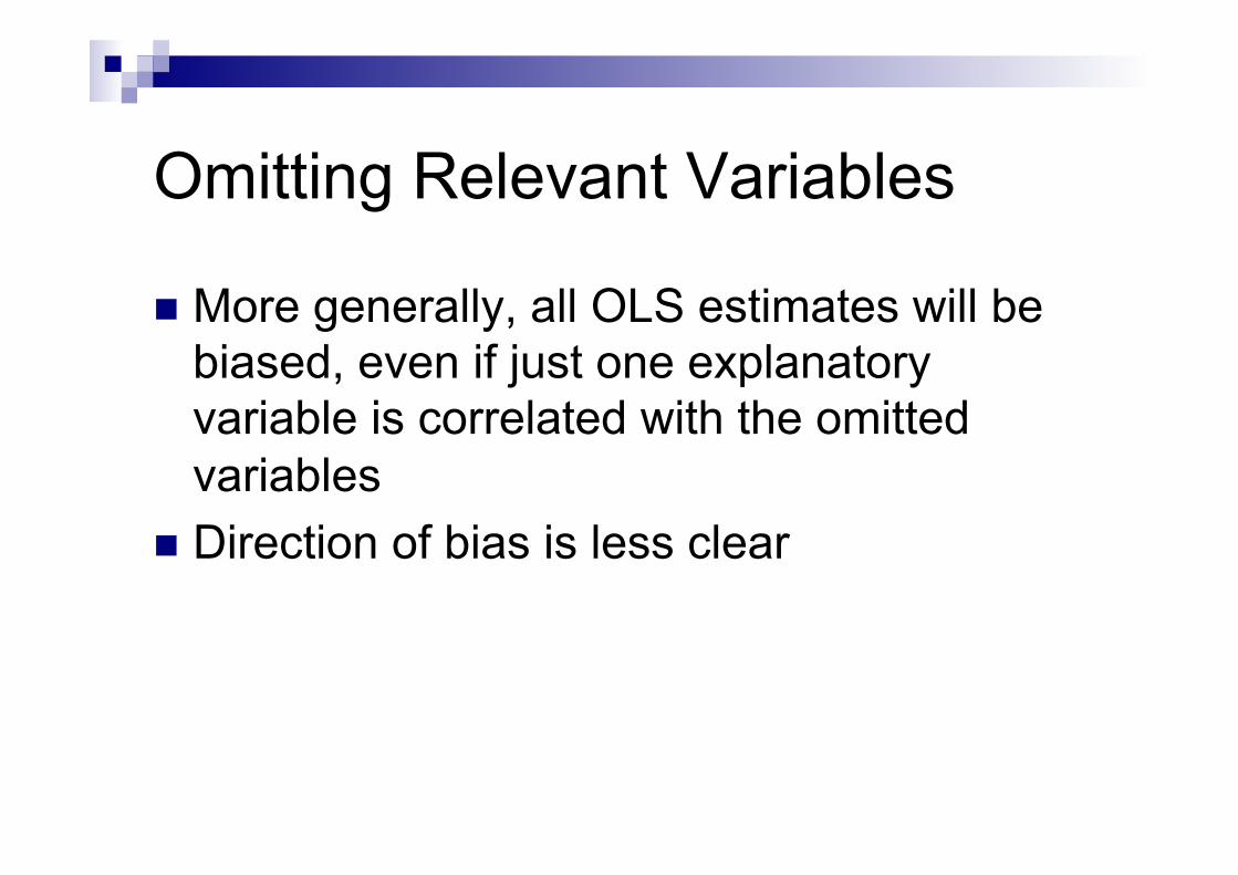
Omitting Relevant Variables
n More generally, all OLS estimates will be biased, even if just one explanatory variable is correlated with the omitted variables
n Direction of bias is less clear
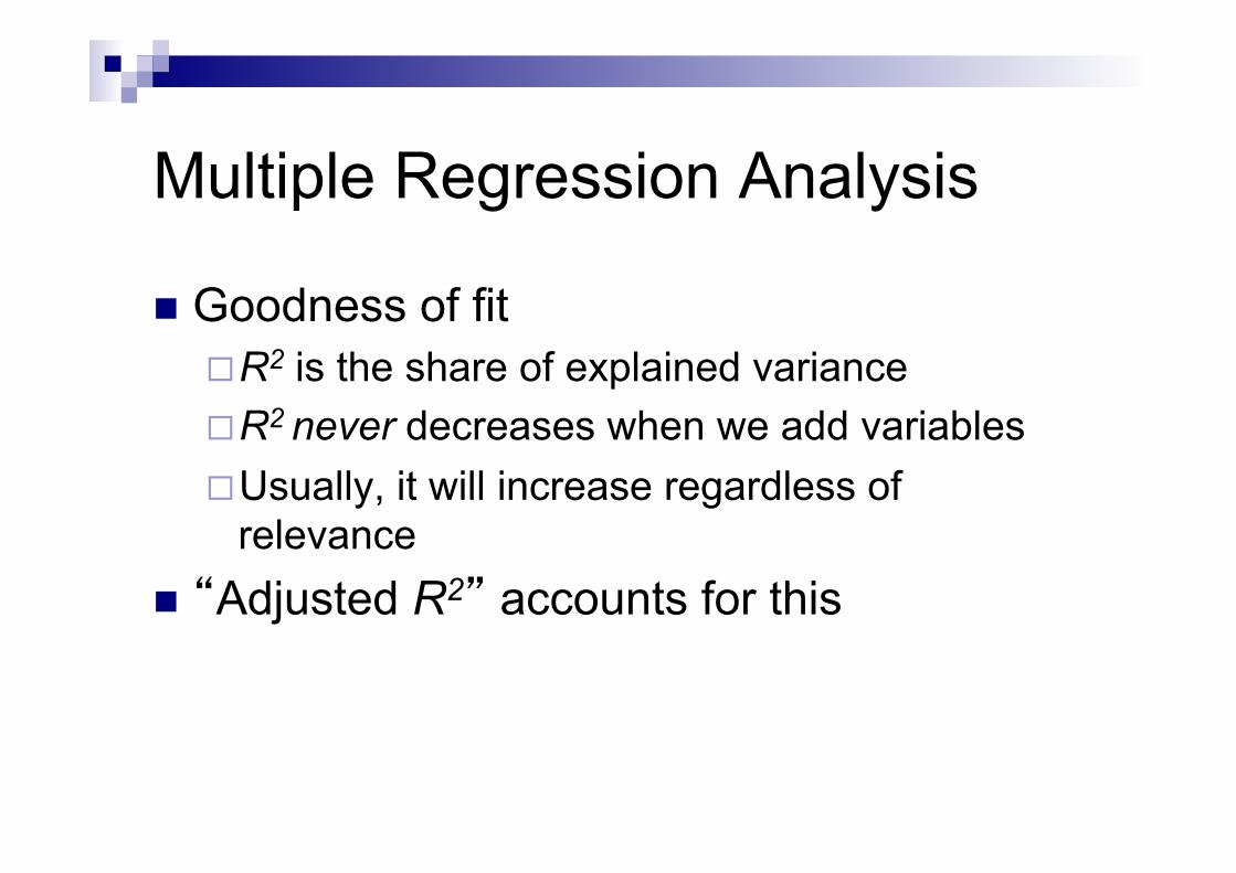
Multiple Regression Analysis
n Goodness of fit ¨ R2 is the share of explained variance ¨ R2 never decreases when we add variables ¨ Usually, it will increase regardless of
relevance n “Adjusted R2” accounts for this
Next time: Interpreting results
n Binary regressors n Other categorical regressors n Categorical regressors as a series of
binary regressors n Quadratic terms n Other interactions n Average Partial Effects

Sessions materials developed by Bill Burke with input from Nicole Mason. January 2012.