Multiple Linear Regression Haze-removal Model

Based on Dark Channel Prior

Binghan Li

226002451

1 Introduction

Images captured in outdoor scenes are usually degraded by haze, fog and smoke.Suffering from poor visibility, reduced contrasts, fainted surfaces and color shift,hazy images will miss many details. Haze removal is highly desired in computa-tional photography and computer vision applications, for that many computervision algorithms can only work well with haze-free images. With the devel-opment of self-driving vehicles, object detection in traffic has developed a lotin recent years. However, in some cities, the traffic environment suffering fromheavy haze will reduce the accuracy of object detection. Because of the distribu-tion difference between the dehazing images and the clean images, only focusingon dehazing algorithm or object detection algorithm is not the best way to im-prove the detection precision. In this project, our purpose is to tackle thiscross-domain object detection problem. The first task is to boost single imagedehazing performance as an image restoration problem. The second task is toimprove object detection accuracy in the presence of haze. Both two tasks willuse the REalistic Single Image DEhazing (RESIDE), which is a new large-scalebenchmark consisting of both synthetic and real-world hazy images.

2 Overview of existing algorithms

2.1 Dark Channel Prior

In computer vision, the classical model to describe the generation of a hazyimage is the atmospheric scattering model:

I (x) = J (x)t(x) + A(1− t(x)) (1)

where I(x) is the observed intensity, J(x) is the scene radiance, A is the at-mospheric light, and t(x) is the medium transmission matrix. The first termJ(x)t(x) on the right-hand side is called direct attenuation, and the secondterm A(1 − t(x)) is called airlight. When the atmosphere is homogeneous, the

1

transmission matrix t(x) can be defined as:

t(x) = e−βd(x) (2)

where β is the scattering coefficient of the atmosphere, and d(x) is the scenedepth, which indicates the distance between the object and the camera.

Given the atmospheric scattering model (1), most state-of-the-art single im-age dehazing algorithms estimate the transmission matrix t(x) and the globalatmospheric light A. Then they recover the clean images J(x) via computingthe transformation of (1):

J (x) =1

t(x)I (x)−A

1

t(x)+ A (3)

To formally describe the observation in DCP [4], the dark channel of animage J is defined as:

J dark(x) = miny∈Ω(x)

(minc

J c(y)) ≈ 0 (4)

Then by minimizing both sides of equation (1), and putting (2) into (1), wecan eliminate the multiplicative term and estimate the transmission t by:

t = 1− miny∈Ω(x)

(minc

J c(y)

Ac ) (5)

However, DCP has many limitations when estimating transmission map t(x)and atmospheric light A, which make DCP fail in some specific cases that arevery common in real world. When the scene object is inherently similar to theair light (e.g., snowy ground or a white wall) over a large local region and noshadow is cast on it, it will underestimate the transmission of these objectsand overestimate the haze layer. So the brightness of the restored image willbe darker than the real haze-free image, which often impacts object detectionnegatively.

2.2 Object detection method

Object detection model has developed a lot in recent years. The developmentfrom R-CNN to Fast R-CNN, from Fast R-CNN to Faster R-CNN, from FasterR-CNN to Mask R-CNN, shows that the deep model will become faster withhigher accuracy. In [10], the authors proposed a cascade of AOD-Net dehazingand Faster-RCNN detection modules to detect object in hazy images. Andtrying different combinations of more powerful dehazing and object detectionmodules in the cascade. What’s more, such a cascade could be subject to furtherjoint optimization.

2

2.2.1 Fast R-CNN

Fast R-CNN is Fast Region-based Convolutional Network. A Fast R-CNN net-work takes as input as entire image and a set of object proposals. The networkfirst processes the whole image with several convolutional and max pooling lay-ers to produce a conv feature map. Each feature vector is fed into a sequenceof fully connected layers that finally branch into two sibling output layers: onethat produces softmax probability estimates over K object classes. Each set of4 values encodes refined bounding-box positions for one of the K classes. [2]

2.2.2 Faster R-CNN

Faster R-CNN consists of two stages. The first stage, called a Region ProposalNetwork (RPN), proposes candidate object bounding boxes. The second stage,which is in essence Fast R-CNN [8], extracts features using RoIPool from eachcandidate box and performs classification and bounding-box regression. Thefeatures used by both stages can be shared for faster inference.

2.2.3 Mask R-CNN

Mask R-CNN extends Faster R-CNN by adding a branch for predicting anobject mask in parallel with the existng branch for bounding box recognitionand classification. It efficiently detects objects in an image while simultaneouslygenerating a high-quality segmentation mask for each instance. [3]

2.2.4 Domain-Adaptive Mask-RCNN

Domain Adaptive Faster R-CNN in [1] is based on the recent state-of-the-artFaster R-CNN model. It designs two domain adaptation components, on imagelevel and instance level, to reduce the domain discrepancy. And inspired bythe Domain Adaptive Faster R-CNN, [7] applied a similar approach to designa domain-adaptive mask-RCNN (DMask-RCNN). The primary goal of DMask-RCNN is to mask the features generated by feature extraction network to beas domain invariant as possible, between the source domain (clean input im-ages) and the target domain (hazy images). Specifically, DMask-RCNN placesa domain-adaptive component branch after the base feature extraction convo-lution layers of Mask-RCNN.

2.3 RESIDE dataset

The REalistic Single Image DEhazing (RESIDE) dataset [6] is the first large-scale dataset for benchmarking single image dehaziang algorithms and includesboth indoor and outdoor hazy images. Further, RESIDE contains both syntheticand real-world hazy images, thereby highlighting diverse data sources and im-age contents. It is divided into five subsets, each serving different training orevaluation purposes. And the test sets address different evaluation viewpoints

3

including restoration quality (PSNR, SSIM and no-reference metrics), subjectivequality (rated by humans), and task-driven utility.

3 Multiple linear regression haze-removal model

After the transmission map t(x) and the Atmospheric Light A are estimated,hazy image can be recovered by:

J (x) =I (x)

t(x)− A

t(x)+ A (6)

In Section II, we already introduced the estimation of transmission map t(x)and the Atmospheric Light A are both based on the hazy images. Althoughmany algorithms attempt to refine the estimations on transmission map t(x),and the Atmospheric Light A, estimations can still generate some unexpecteddeviations. And this kind of errors are normally impossible to eliminate. Nowwe introduce the multiple linear regression model to optimize the atmosphericscattering model (6). Multiple linear regression is the most common form oflinear regression analysis. As a predictive analysis, multiple linear regressionis used to explain the relationship between one continuous dependent variableand two or more independent variables. When we train with thousands ofsynthetic images and haze-free images, the scene radiance J(x), which is also theRGB pixel of haze-free image, can be regarded as the the continuous dependent

variable. For each image, after we estimate t(x) and A by original DCP, I (x)

t(x),

At(x)

and A in (6) can be regarded as three independent variables, where I(x) is

the pixel of hazy image. Then both two parameters t(x) and A together withthe pixels of input images and target images can be simplified to a predictionproblem with multiple linear regression model, which describes how the meanresponse J(x) changes with the three explanatory variables:

J (x) = w0I (x)

t(x)+ w1

A

t(x)+ w2A + b (7)

Then we implement Stochastic Gradient Descent (SGD) to our multiplelinear regression model, which is one of the most widely used algorithms tosolve optimization problems. The Outdoor Training Set (OTS) of RESIDEdataset provides 8970 outdoor haze-free images. For each haze-free image, OTSalso provides about 30 synthesis hazy images with haze intensity from low tohigh. Different haze intensity means a lot to our multiple linear regression haze-removal model, because we don’t expect that our algorithm can only performgood on hazy images with fixed haze intensity. When we train our model onOTS, we refer haze-free images as target images J , refer synthesis images asinput images I, take the images recovered from our model as output images Jω.Then (7) can be re-formulated as:

Jω(x) = w0x 0 + w1x 1 + w2x 2 + b (8)

4

For that I(x) and A are both defined based on RGB color channels, the dimen-sion of three weights and bias is (3,1), aiming to refine the parameters fromall three color channels. And the deviations of the output images Jω from thetarget images J are estimated by mean-squared error (MSE):

MSE = (J − Jω)2 (9)

By training our model, we try to find the optimal weights and bias thatminimize the mean-squared error.

• Define the cost function of our model based on (9):

L(ω) =1

2n

n∑i=1

(J (i) − J (i)ω )2 (10)

• For each image in training set, we repeatedly update three weights via:

ωk = ωk − α∂

∂ωL(ω)xk (11)

where α is the learning rate, and k ∈ 0, 1, 2.

• Since the derivative of cost function can be computed via (10), Equation(11) can be simplified as:

ωk = ωk − α1

n

n∑i=1

(J (i) − J (i)ω )xk (12)

• For each image in training set, we repeatedly update the bias via:

b = b− α 1

n

n∑i=1

(J (i) − J (i)ω ) (13)

And after we get the optimal weights and bias, they can be simply addedto traditional DCP. What’s more, the multiple linear regression model will notmodify the inner theory of any state-of-the-art dehazing algorithm. Our modelcan be applied to further improve the performance of some state-of-the-art de-hazing algorithms that optimize the estimations of t(x) and A.

4 Results

In this section, by demonstrating our dehazing results on several groups of hazyimages as well as comparing the PSNR and SSIM value, we show the betterperformance of our model over DCP and other dehazing algorithms. And wecombine our dehazing model with DMask R-CNN object detection model, totest the mAP value on RTTS dataset. Compared with the highest mAP valueso far, our result is almost the same to it.

5

4.1 Experiment setup

Most recently, a benchmark dataset of both synthetic and real-world hazy im-ages provided in [6] for dehazing problems are introduced to the community. Inour experiment, the Synthesis Object Testing Set (SOTS) in RESIDE dataset isused to test the dehazing performance of our method. Our algorithm focuses onrecovering outdoor hazy images, therefore, we won’t evaluate the performanceon recovering the 500 synthetic indoor images in SOTS. And the Real-worldTask-Driven Testing Set (RTTS) is used to test the precision of object detec-tion in haze.

In the training phase, 8000 haze-free images and corresponding synthetichazy images in Outdoor Training Set (OTS)[6] are used to train our multi-ple linear regression haze-removal model. In the testing phase, 500 outdoorhaze-free images and 500 outdoor synthetic hazy images in Synthetic ObjectiveTesting Set(SOTS) are tested using the well trained model. We compare theperformance with original DCP from both the average SSIM and PSNR, and wealso list the comparison of recovered images between our algorithm and DCP toprove that the multiple linear regression haze-removal model can overcome theweakness of DCP.

4.2 Experiment results on SOTS

In Fig. 1, We demonstrate the performance of multiple linear regression haze-removal model from the difference observed through recovered images via orig-inal DCP and our improved model. Fig. 1 (a) shows a synthetic hazy imageselected from SOTS, and Fig. 1 (b) shows its haze-free image. Fig. 1 (c) showsthe recovered image via original DCP. We can easily observe that the colordistortion in sky region and non-sky region performs darker than its haze-freeimage. Fig. 1 (d) shows the recovered image via our model. Compared withthe haze-free image, the haze is almost completely removed and the sky regionseems more natural. The high similarity is obvious through observation.

In Table 1, we compare our results with several state-of-the-art method withaverage SSIM and average PSNR. As we mentioned in Section III, PSNR andSSIM together can compare the image quality and similarity between recoveredimages and haze-free images. Since we want to apply our improved model ontraffic dehazing problems, we only compare the results on 500 outdoor imagesin SOTS in this table. All the results of other algorithms come from [6]. Whencompared with well-recognized state-of-the-art dehazing algorithms and deeplearning methods, our proposed model achieves reasonably good PSNR valueand obtains the highest SSIM value. The results show the effectiveness of ourmodel on dehazing outdoor images.

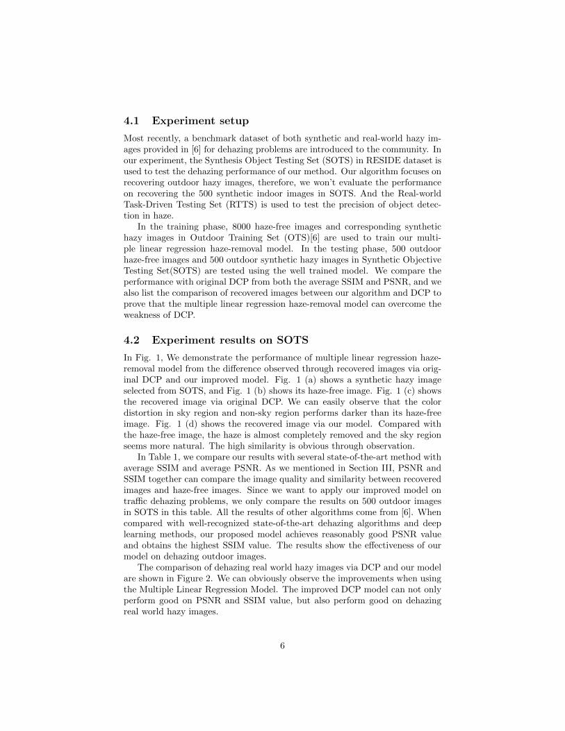
The comparison of dehazing real world hazy images via DCP and our modelare shown in Figure 2. We can obviously observe the improvements when usingthe Multiple Linear Regression Model. The improved DCP model can not onlyperform good on PSNR and SSIM value, but also perform good on dehazingreal world hazy images.

6

(a) Synthetic hazy image (b) Haze-free image

(c) Recovered image by DCP (d) Recovered image by our model

Figure 1: Comparison on synthetic hazy image

7

(a) Hazy image (1) (b) Hazy image (2)

(c) Recovered image (1) via DCP (d) Recovered image (2) of via DCP

(e) Recovered image (1) via our model (f) Recovered image (2) via our model

Figure 2: Comparison on real-world nature hazy images

8

500 outdoor imageDehazing method name PSNR SSIMImproved DCP model 23.84 0.9411

DCP 18.54 0.7100FVR 16.61 0.7236BCCR 17.71 0.7409GRM 20.77 0.7617CAP 23.95 0.8692NLD 19.52 0.7328

DehazeNet 26.84 0.8264MSCNN 21.73 0.8313AOD-Net 24.08 0.8726

Table 1: Average SSIM and PSNR comparison between different dehazing meth-ods on 500 outdoor synthetic image in SOTS.

4.3 Experiment results on RTTS

Some experiments on object detection in haze based on RTTS dataset have beenmade in [5] [6] [7]. From the comparison of the mAP value among Faster R-CNN, Mask R-CNN and Domain-Adaptive Mask-RCNN combined withe severaldehazing algorithms, we pick the Domain-Adaptive Mask-RCNN in [7] with thebest performance. Firstly, we use the original DCP with Guided Filter andour Multiple Linear Regression Model with the best performance to dehazeeach hazy image in RTTS dataset separately and save the dehazed images intotwo folders named ”result” and ”9411result”. We use the pretrained Domain-Adaptive Mask-RCNN to run the two dataset we added.

From the results in Table 2, after using the best performance Multiple LinearRegression Model to dehaze images in RTTS, we get mAP value that is only0.1% lower than that of ”MSCNN + DMask R-CNN2”. And the mAP value of”MSCNN + DMask R-CNN2” is the highest among all object detection in hazemodels that tested on RTTS dataset.However, compared with the PSNR and SSIM values of MSCNN in the lastexperiment, Multiple Linear Regression Model and AOD-Net outperform theMSCNN a lot. We can simply conclude that the higher PSNR value and SSIMvalue don’t equal to higher mAP value on object detection in haze. From theprevious discussion about the limitaion of original DCP, we know the dehazed

9

mAP valuesFramework mAP(%)

Mask R-CNN 61.01DMask R-CNN1 61.21DMask R-CNN2 61.72

AOD-Net + DMask R-CNN1 60.21AOD-Net + DMask R-CNN2 60.47MSCNN + DMask R-CNN1 62.71MSCNN + DMask R-CNN2 63.36DCP + DMask R-CNN2 62.78

Multiple Linear Regression Model + DMask R-CNN2 63.25

Table 2: mAP values comparison among different models

image will be darker than normal scenes due to the rough estimations of t(x). Iused to suspect that will reduce the precision of object detection a lot. From theresults in Table 2, orignal DCP with Guided Filter even performs much betterthan AOD-Net. One advantage of DCP is that it can remove heavy haze. Wehave a assumption that the amount of haze removed is more important thanthe effect of restored image becoming darker when we apply dehazing algorithmwith object detection model. That can explain why original DCP with worseperformance can outperform AOD-Net with better performance on dehazing.

5 Conclusion and Discussion

From the three experiments, we conclude that The Multiple Linear RegressionDCP Model gets the highest SSIM value and reasonable PSNR value, performsvery good on dehazing real world hazy images and gets almost the highestmAP value when combined with object detection model. Overall, it’s muchbetter than other dehazing model so far. Since the MSCNN dehazing modelgets the highest mAP value on object detection in haze experiment with worseperformance on PSNR value and SSIM value compared with AOD-Net and ourimproved model, we can not only focusing on improving the PSNR value andSSIM value of an dehazing algorithm. We also need to study what kind ofquality of dehazed images can boost the performance on object detection inhaze.

References

[1] Yuhua Chen, Wen Li, Christos Sakaridis, Dengxin Dai, and Luc Van Gool.Domain adaptive faster r-cnn for object detection in the wild. In Proceedings

10

of the IEEE Conference on Computer Vision and Pattern Recognition, pages3339–3348, 2018.

[2] Ross Girshick. Fast r-cnn. In Proceedings of the IEEE international confer-ence on computer vision, pages 1440–1448, 2015.

[3] Kaiming He, Georgia Gkioxari, Piotr Dollar, and Ross Girshick. Mask r-cnn.IEEE transactions on pattern analysis and machine intelligence, 2018.

[4] Kaiming He, Jian Sun, and Xiaoou Tang. Single image haze removal usingdark channel prior. IEEE transactions on pattern analysis and machineintelligence, 33(12):2341–2353, 2011.

[5] Boyi Li, Xiulian Peng, Zhangyang Wang, Jizheng Xu, and Dan Feng. Aod-net: All-in-one dehazing network. In Proceedings of the IEEE InternationalConference on Computer Vision, volume 1, page 7, 2017.

[6] Boyi Li, Wenqi Ren, Dengpan Fu, Dacheng Tao, Dan Feng, Wenjun Zeng,and Zhangyang Wang. Reside: A benchmark for single image dehazing.arXiv preprint arXiv:1712.04143, 2017.

[7] Yu Liu, Guanlong Zhao, Boyuan Gong, Yang Li, Ritu Raj, Niraj Goel,Satya Kesav, Sandeep Gottimukkala, Zhangyang Wang, Wenqi Ren, et al.Improved techniques for learning to dehaze and beyond: A collective study.arXiv preprint arXiv:1807.00202, 2018.

[8] Shaoqing Ren, Kaiming He, Ross Girshick, and Jian Sun. Faster r-cnn: To-wards real-time object detection with region proposal networks. In Advancesin neural information processing systems, pages 91–99, 2015.

11