multiple kernel learning for stock price direction prediction · 1.1 stock market 9 1.1.1 technical...
TRANSCRIPT

Multiple Kernel Learning for Stock Price Direction
Prediction
Dissertation
Submitted in partial fulfillment of the requirement for the degree of
Master of Technology in Computer Engineering
By
Amit Kumar Sirohi
MIS No: 121222014
Under the guidance of
Dr. Vahida Attar
Department of Computer Engineering and Information Technology
College of Engineering, Pune
Pune – 411005
June, 2014
DEPARTMENT OF COMPUTER ENGINEERING AND
INFORMATION TECHNOLOGY,

ii
COLLEGE OF ENGINEERING, PUNE
CERTIFICATE
This is to certify that the dissertation titled
Multiple Kernel Learning for Stock Price Direction Prediction
has been successfully completed
By
Amit Kumar sirohi
MIS No: 121222014
and is approved for the partial fulfillment of the requirements for the degree of
Master of Technology, Computer Engineering
Dr. Vahida Attar
Project Guide,
Department of Computer Engineering
and Information Technology,
College of Engineering, Pune,
Shivaji Nagar, Pune-411005.
Dr. J. V. Aghav
Head,
Department of Computer Engineering
and Information Technology,
College of Engineering, Pune,
Shivaji Nagar, Pune-411005.
June 2014

3
Acknowledgments
I express my deepest gratitude towards my guide Prof. Dr. Vahida Attar for her constant help
and encouragement throughout the project and also for providing me infrastructural facilities to
work in. I have been fortunate to have a guide who gave me the freedom to explore on my own
and at the same time helped me plan the project with timely reviews and constructive comments,
suggestions whenever required. A big thanks to her for having faith in me throughout the project
and helping me walk through the new avenues of research papers and publications.
I would like to thank Dr. Aniruddha Pant for his continuous guidance throughout the project; he
has constantly encouraged me to remain focused on achieving my goal. I also like to convey my
sincere gratitude to Dr. J. V. Aghav(HOD), all faculty members and staff of Department of
Computer Engineering and Information Technology, College of Engineering, Pune for all
necessary cooperation in the accomplishment of dissertation. I would take this opportunity to
thanks all those teachers, staff and colleagues who have constantly helped me grow, learn and
mature both personally and professionally throughout the process. Last but not least, I would
like to thank my family and friends, who have been a source of encouragement and inspiration
throughout the project.
Amit Kumar Sirohi
College of Engineering, Pune

4
ABSTRACT
In financial market, stock market plays a vigilant role. To forecasts the estimation of worldwide
stock market is not an easy work. Unstable and assumptive aspects of the securities make it hard
to predict the next day stock prices. There is no particular indicator for financial forecasting but
there are many technical indicators to elaborate a stock trend.
In this Project, we implement a combination of different base kernels to predict the direction of
stock prices going up or down in future, which comprises a 2-tier framework.
In first tier, we prepare the data and compute some technical indicators and normalize a
data set into a MKL data representation.
In second tier, design a model which has three sub-tasks :
Construct different base kernels on the extracted featured set.
For the different base kernels, the weights are first learned and then tuned,
and then these base kernels are combined.
Performing Multiple kernel Learning through walk forward approach and
predict the movement of daily stock prices going up or down
As compared to single kernel methods, Multiple Kernel Learning methods are more accurate and
there are fewer chances of wrong prediction. It will be beneficial for stock market as compared
to other existing prediction methods.

5
List of Figures
1.1 Separating Hyper plane 13
1.2 Maximal separating hyper plane 15
2.1 The Scope of Literature Review 18
3.1 Proposed Model 20
4.1 Methodology 21
4.2: Data Partition 22
4.3 Preparation of Vector sets for MKL and SVM 23
4.4 Walk Forward Method. 25
4.5 Confusion Matrix 26
5.1.1. Analysis of different methods on F Data with window size 450 31
5.1.2 Analysis of different methods on F Data with window size 750 32
5.1.3 Analysis of different methods on F Data with window size 950 32
5.1.4. Analysis of different methods on F Data at Norm 1 33
5.1.5. Analysis of different methods on F Data at Norm 1.2 33
5.1.6. Analysis of different methods on F Data at Norm 1.3 34
5.1.7 Analysis of different methods on F Data at Norm 1.6 34
5.1.8 Analysis of different methods on F Data at Norm 1.75 35
5.2.1 Analysis of different methods on N Data with window size 450 39
5.2.2 Analysis of different methods on N Data with window size 750 40
5.2.3 Analysis of different methods on N Data with window size 950 40
5.2.4 Analysis of different methods on N Data at Norm 1 41
5.2.5 Analysis of different methods on N Data at Norm 1.2 41
5.2.6 Analysis of different methods on N Data at Norm 1.3 42
5.2.7 Analysis of different methods on N Data at Norm 1.6 42

6
5.2.8 Analysis of different methods on N Data at Norm 1.75 43

7
List of Tables
4.1 Experimental Data 22
4.2 Details of each method 24
5.1.1: MKL-1 results on F Data with windows size 450 27
5.1..2 MKL-1 result on F Data with window size 750 27
5.1.3 MKL-1 result on F Data with window size 950 27
5.1.4 MKl-2 results on F Data with window size 450 28
5.1.5 MKl-2 results on F Data with window size 750 28
5.1.6 MKl-2 results on F Data with window size 950 28
5.1.7 MKl-3 results on F Data with window size 450 28
5.1.8 MKl-3 results on F Data with window size 750 29
5.1.9 MKl-3 results on F Data with window size 950 29
5.1.10 MKl-4 results on F Data with window size 450 29
5.1.11 MKl-4 results on F Data with window size 750 29
5.1.12 MKl-4 results on F Data with window size 950 30
5.1.13 MKl-5 results on F Data with window size 450 30
5.1.14 MKl-5 results on F Data with window size 750 30
5.1.15 MKl-5 results on F Data with window size 950 30
5.1.16 . SVM results on F Data 31
5.2.1 MKL-1 results onN Data with windows size 450 35
5.2.2 MKL-1 result on N Data with window size 750 35
5.2.3 MKL-1 result on N Data with window size 950 36
5.2.4 MKl-2 results on N Data with window size 450 36
5.2.5 MKl-2 results on N Data with window size 750 36
5.2.6 MKl-2 results on N Data with window size 950 36

8
5.2.7 MKl-3 results on N Data with window size 450 37
5.2.8 MKl-3 results on N Data with window size 750 37
5.2.9 MKl-3 results on N Data with window size 950 37
5.2.10 MKl-4 results on N Data with window size 450 37
5.2.11 MKl-4 results on N Data with window size 750 38
5.2.12 MKl-4 results on N Data with window size 950 38
5.2.13 MKl-5 results on N Data with window size 450 38
5.2.14 MKl-5 results on N Data with window size 750 38
5.2.15 MKl-5 results on N Data with window size 950 39
5.2.16 . SVM results on N Data 39

9
Contents
Certificate 2
Abstract 3
List of Figures 4
List of Tables 5
1 Introduction 9
1.1 Stock market 9
1.1.1 Technical Analysis 10
1.1.2 Fundamental Analysis 10
1.2 Support Vector Machine 11
1.3 Multiple Kernel Learning 14
1.4 Motivation 16
1.5 Thesis Objectives and Thesis Outlines 16
2. Literature Survey 17
2.1 Stock Market Movements 17
2.1.1 Efficient Market Hypothesis 17
2.1.2 Random Walk Theory 18
2.2 Literature review of Technical analysis 18
2.3 Literature review of Some Trading models 19
2.4 Literature review of Multiple Kernel Learning 21
3 Problem Statement 23
3.1 Problem Definition 23
3.2 Proposed Methodology 23
4 Experimental setup 25
4.1 System Specification 25
4.2 Data collection and Data preprocessing 26
4.3 Model Training 28
4.4 Evaluation Metrics 29
5 Results and Analysis 31

10
5.1 F Data Results 31
5.2 N Data Results 39
6 Conclusion and Future Work 48

11
Chapter1
Introduction
1.1 Stock Market
In financial market, stock market prediction is a substantial issue in mathematics, finance
engineering due to its financial hide and seek. A huge amount of money is invested in stock
market, this is one of the reasons why stock market can be seen on peaks, but still financial
market is unpredictable, still you can't predict what will be next day price. People have studied a
lot to evaluate and forecast the stock price, involving statistics and other prediction method based
on ancestral stock price or volume abstract and technical analysis. For the frugality of a country,
share market plays a substantial role. It is the only places where investor can buy share and get
benefited, at many have become millionaire in stock market. .and also company can also raise
their fund without taking any loan or without any interest. The stock market is marking an
substantial augmentation to frugatile growth, is one of the most vigorous area in the monetary
system. Buyers and sellers of stocks in the stock market securities, bonds, debentures etc. can
enter into a purchase and sale transaction or we can say stock market is a Scaffold for dealing
certain collateral and descendants. In addition, through this community concern to accrete
possessions for their companies and corporate business ventures, enabling entrepreneurs have a
substantial role.
In many areas of machine learning algorithm for analyzing price pattern, a lot of studies or work
has been done for forecasting stock prices and change in index. Today mostly all the prediction
was mostly based on intelligence business system. Which help them in forecasting prices based
on various conditions and salutation, which help in taking quick investment decision? Stock
market changes dynamically and there are quick changes. .in a single moment only stock price
can show huge variation. Company not only gives share to the investor but it also gives the
ownership of the company. Many people are still confused about stock market. Some people
believe that investing money in stock market is like gambling. The people, who have this
thinking, actually don’t understand stock market. It’s not gambling, it’s an investment and
analysis finding patterns in the past time series data. Through stock market, a person can grow a

12
small amount of money into a large sum. A person can become wealthy without starting a
business with huge investment. Stock market is an accretion of buying and selling.
Changes are very quick in the stock market due to essential disposition of dominion because of
brew of criterions(closing price of previous day, p/e ratio etc.) and some factors that are not
known like (Election Results ,Rumors etc) A good trader is the one who can estimate the rise or
fall of the stock market. .and he buy the shares before its rate gets high and sell his share before
the share fall. In short is able to get maximum benefit. .although it is very difficult to do correct
prediction but a correct or accurate forecasting of stock market can give you lot of gain and in
the blinking of eye sometimes you can become millionaire.
Stock market is unpredictable as it’s very difficult to predict the stock price of any stock. By
doing some analysis on the market, researchers find some patterns in the historical data. There
are two types of analysis in the market – fundamental analysis and technical analysis.
1.1.1 Fundamental Analysis
These are anxious with the companies that influence the stock itself. They estimate on the basis
of a company’s performance in the past and also the integrity of its account. Many performance
ratios like P/E ratio are erected to aid the fundamental analysis with estimating the existence of
the stock. One of most famous Fundamental analyst is Warren Buffet. It is made on fact criteria
that company invest the money of the people; if company is getting profit the company shares
the profit with its share holders.
1.1.2 Technical Analysis
In stock market analysis there are two approaches first approach includes analysis of graphs
where analysts try to find out certain patterns that are followed by stock but this approach is very
difficult and very complex. In second approach analyst make use of quantitative parameters like
trend indicators, daily ups and downs, highest and lowest values of a day, volume of stock,
indices, put/call ratios, etc. It also includes some averages which is nothing more than mean of
prices for particular window. Simple Moving Average (EMA) of last n days and Exponential
Moving Average (EMA) where price of recent days has more weight in average. Analyst tries to
find out some mathematical formula which can map this input to the desired output. That why

13
most of the machine learning techniques prefer technical analysis data over fundamental analysis
data as input to system.
1.2 Support Vector Machine
SVM is the state-of-art approach for classification problems [6, 3] SVM is a supervised learning
method used for classification, regression and other tasks. Basic principle is that given a set of
training data points, the task is to divide these training data points into two classes by finding the
separating hyper plane which maximizes the distance or margin to the nearest training data
points of any class (called functional or geometric margin). This will be ensuring the
classification of unseen points to be better that is a better generalization. Clearly explain by the
figure 1.1, there are three hyper planes shown in the diagram. S3 hyper plane does not classify
well all the training data points. S1 classifies all the training data points but it is not at the
maximum margin from their nearest training data points. S2 hyper plane classifies all the training
data points well and it is the maximum margin separating hyper plane.
The key characteristics of SVM are that they simultaneously maximize the functional margin and
minimizes the structural risk error. The advantages of SVM are:
SVM method is efficiently work in high dimensional space.
Figure1.1. Separating Hyper planes
14
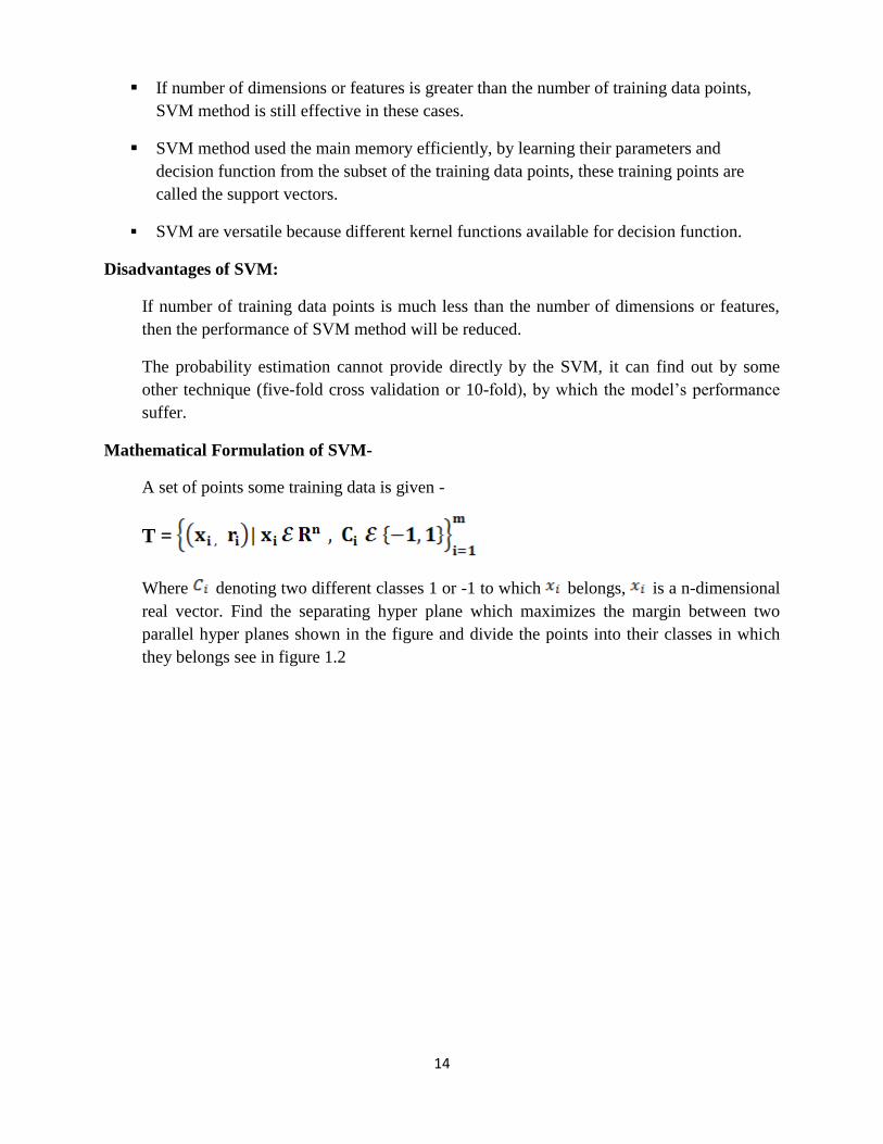
If number of dimensions or features is greater than the number of training data points,
SVM method is still effective in these cases.
SVM method used the main memory efficiently, by learning their parameters and
decision function from the subset of the training data points, these training points are
called the support vectors.
SVM are versatile because different kernel functions available for decision function.
Disadvantages of SVM:
If number of training data points is much less than the number of dimensions or features,
then the performance of SVM method will be reduced.
The probability estimation cannot provide directly by the SVM, it can find out by some
other technique (five-fold cross validation or 10-fold), by which the model’s performance
suffer.
Mathematical Formulation of SVM-
A set of points some training data is given -
T =
Where denoting two different classes 1 or -1 to which belongs, is a n-dimensional
real vector. Find the separating hyper plane which maximizes the margin between two
parallel hyper planes shown in the figure and divide the points into their classes in which
they belongs see in figure 1.2

15
The equation of any hyper plane is given as –
w is a normal vector perpendicular to the hyperplane . The offset of the hyperplane from
the origin in the direction of normal vector w is calculated by the parameter . To
maximize the margin , choose a suitable values of normal vector w and b. In the figure see
the two parallel hyperplanes , these can be represented as:
, and
If given data is linearly separable, select two parallel hyper planes is such a way that no
point lies between them. Distance between two parallel hyper planes is find out
by geometry, minimize to maximize the distance between two parallel hyper planes.
Primal Form
In the above section, discussed about optimization problem is difficult to optimize due to its
dependency on the absolute value of . In mathematical form actual reason is that, it’s a
problem of non-convex optimization which is very difficult to solve. Favorably it is
Figure1.2: Maximal separating hyper plane

16
conceivable to change the equation by replacing with without alter the
solution of the equation the minimum of the original and modified equation have the equal
value of w and b. It is a quadratic programming (QP) optimization
Minimize :
Subject to:
For mathematical convenience the factor is used. This problem can now be solved by standard
quadratic programming techniques and programs.
The rule of classification in corrupted or unconstrained form disclose the maximum separating
hyper plane, so the classification problem is a function of only support vectors, training points
that lie on the margin . The dual of the SVM shows as:
Maximize:
Subject to:
Where a weight vector in terms of the training set conditions for forming a duple enactment in α
terms.
Soft Margin
In 1995, Corinna Cortes and Vladimir Vapnik gave a Maximum modified margin which allows
misclassified examples. No such hyper plane exist which can divide "yes" or " no" class but soft
margin hyper plane choose that hyper plane can split examples cleanly as possible while still
maximizing the distance.

17
1.3Multiple Kernel Learning
Multiple Kernel learning is a method which manage with the issue of a kernel choice [2][3]. This
technique decreases the risk of wrong selection of a kernel to some extent by adopting a set of
kernels and for each kernel determined its weight such that every prediction are built on
weighted aggregate of various kernels. The multiple kernels increase the performance of the
model and interpretability of the results.
Suppose (m=1,….M) are M positive definite kernels on the same input data .X,
………(1)
Where are weights of sub-kernel m, and ξ represents the loose variables and C is used to
control the generalization error of the classification. The resulting kernel,
………..(2)
It has been known that L1 norm regularization tends to produce sparse solutions which means
during the learning most kernels are assigned virtually zero weights. This behavior may not
always be desirable because the information carried in the kernels that get zero weights is
completely discarded. A non-sparse version of multiple kernels is proposed by KLoft et al.in [7],
where an L2 norm regularization is imposed instead of L1 norm.
Algorithm Simple norm MKL wrapper-based training algorithm. The analytical updates of
θ and the SVM computations are optimized simultaneously.
Input: feasible α and β
While optimality conditions are not satisfied do
Compute α (SVM Parameter)
Compute for all m=1,……..M according to equation (1)

18
Update β according to equation (2)
End while

19
1.4 Motivation
Millions of the people in the world are earning a lot from a stock market. Capitalist wants to earn
more and more to get high dividends whole day, they monitor all the stocks of the companies, as
every moment they have hope to earn a profit, they seek for every possible opportunity. Broker
is a middle man between buyer and seller. But their job is also not that much easy. Daily brokers
have to keep eye on every activity of the company. They keep track on company’s performance,
any political issues that can affect the frugality, international market etc. Because on the basis of
their experience or research only or using their sixth sense they buy or sell shares Its very
difficult or we can say nobody is able to come. However overall trend i.e. weekly or monthly can
be predicted by some great minds to which the challenge of prediction increases. Infect there are
many fields like financial organization is mutual funds they want to spend maximum in the stock
market as to get maximum profit. These companies invest money on the basis of prediction
model. Exact predictions are still not possible that’s why people say stock market is
unpredictable. If broker or any financial organization is able to detect or forecast the stock
market, they will be able to gain maximum profit and stock market will be of great value to
them. Now days everywhere people are working to predict the stock prices, they are making
trading models, used machine learning techniques and data mining algorithms to predict the
behavior of stock market. After a lot of research still there is no model which can do accurate
prediction of stock market that’s why still it is an active area for research.
1.5 Thesis Objectives and Thesis Outlines
The Objective of this thesis is to increasing the performance of stock prediction model , As we
know stock market is unpredictable. In this experiment we will make several combination of
kernels, using different norms and window sizes to find norms which work accurately for
financial data. In order to predict future stock market more precisely
Thesis is organized into 6 chapters, chapter 1 describes about the stock market, Technical
analysis, fundamental analysis and then some background of Machine learning techniques.
Chapter 2 is all about the literature survey which describes the various trading models used
different technique, comparison of Support vector machine with other techniques, and different
norms for MKL. Chapter 3 describes problem statement and proposed solution. For chapter 4
explain about the experimental work we have carried out and in chapter 5 show their results and
analysis. Chapter 6 for conclusion and future work we listed respectively.

20
Chapter 2
Literature Survey
2.1 Stock Market Movement
To eradicate advantageous patterns and forecast their movement, stock market has been
lucubrating over and over again. Researchers have a great appeal towards stock market
prediction, many scientists and researchers have made many models and done many experiments
but they were not able to predict stock price movement accurately. To forecast the stock price
movement, there are many approaches and stock market analysts have applied many prediction
techniques to forecast the stock market movement. Here we are describing two substantial
theories for stock market prediction. On the basis of these theories , for financial market two
accustomed avenues have transpired - fundamental analysis and technical analysis.
Theories of Stock market prediction- When we are forecasting the future prices of stock
substantial theories are available. (1) Efficient Market hypothesis (EMH) it is introduced in 1964
by Famma. (2) Random Walk Theory it is introduced by Malkei in 1996. Now we will see the
differentiation between two common theories.
2.1.1 Efficient Market Hypothesis (EMH)
EFFICIENT MARKET HYPOTHESIS (EMH) Famma's contribution in predicting stock price
movement is significant. Today's stock market movement flashes the absorption of all the
available information. So, we can say that by the information we have only cannot predict the
stock market movement. When new information is entered, it get balanced with the previous
information and quickly removes the prior prediction and gives a new prediction. In short we can
say by the information we had in the past and information we have in the present, we can predict
the future stock price movement. Famma's further said that his theory can be broken into three
forms- Weak, strong and semi strong.
In weak EMH only the archival information and past price is inherent in the contemporary price.
It can be used at any kind of prediction because it is based on the random walk in the consecutive
changes having zero correlation. The semi strong form is same as weak EMH but it also has
21
trading information like fundamental data (profit chances and sales prediction) and volume data.
In the strong form include archival information, private information and also the insider
information.
There was a time when weak and semi strong EMH has been supported by a lot of researchers
but now the publisher report says that the prediction from the EMH is far from the contemporary
price. In a way, this hypothesis is considered false to such an extent. And about the strong form
of EMH , it has also been difficult due to shortage of abstract or data
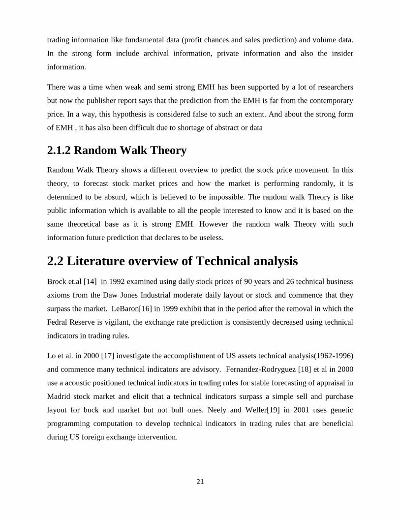
2.1.2 Random Walk Theory
Random Walk Theory shows a different overview to predict the stock price movement. In this
theory, to forecast stock market prices and how the market is performing randomly, it is
determined to be absurd, which is believed to be impossible. The random walk Theory is like
public information which is available to all the people interested to know and it is based on the
same theoretical base as it is strong EMH. However the random walk Theory with such
information future prediction that declares to be useless.
2.2 Literature overview of Technical analysis
Brock et.al [14] in 1992 examined using daily stock prices of 90 years and 26 technical business
axioms from the Daw Jones Industrial moderate daily layout or stock and commence that they
surpass the market. LeBaron[16] in 1999 exhibit that in the period after the removal in which the
Fedral Reserve is vigilant, the exchange rate prediction is consistently decreased using technical
indicators in trading rules.
Lo et al. in 2000 [17] investigate the accomplishment of US assets technical analysis(1962-1996)
and commence many technical indicators are advisory. Fernandez-Rodryguez [18] et al in 2000
use a acoustic positioned technical indicators in trading rules for stable forecasting of appraisal in
Madrid stock market and elicit that a technical indicators surpass a simple sell and purchase
layout for buck and market but not bull ones. Neely and Weller[19] in 2001 uses genetic
programming computation to develop technical indicators in trading rules that are beneficial
during US foreign exchange intervention.

22
Kavajecz and Odders-White [20] in 2004 demonstrate that technical analysis abstraction assist
and detention levels coexist with crest in declination on the limit order book and order book
arousing moderate prediction are advisory concerning declination.
2.3 Literature review of some trading models
In Han & Yien[23] using SVM trained by LC perceptron a multilayer back propagation
algorithm is studied in comparison with the financial forecasting . The subject of Prodera Was
the S&P 500 daily index in the Chicago Mercantile. SVM program better than BP. As such there
is no organized or precise way to select free criterion or guidelines of SVM. SVMs abstraction
absurdities with respect to the free criterion are inquisted in this experiment. According to this
article they have little effect on the clarification of solution.
For adumbrating of four chief evidence in Kuala lumper stock exchange by CH.et.al[25] SVR
model was considered in detail. RBF kernels and SVR with polynomials were distinguished and
consummate that the accomplishment of polynomial kernel is superior to RBF. In addition,
FFNN with BP was correlated with SVR. Polynomial kernel with SVR was found to be better
than FFNN too.
In the year 2000, Theodre [26] compared FFNN with SVR to forecast the stock prices of AOL,
YAHOO and IBM. They also applied the different model of SVRs and FFNNs. IOL models and
best values of MSE for the SVM and FFNN were 2.0573 and 2.3512 respectively. MSE for IBM
for SVM and FFNNs, with a great margin AOL and YAHOO came out to be winners, while
SVCs FFNNs beat IBM with a small margin.
The use of FFNN financial forecast report, along with original series, technical indicators were
used as reported in which ameliorated the performance. Even better Results than basis
information about the companies is also reported [21, 22 ] .
Chi & Liang[24,25] use hidden Markov model to predict stock data in real time at speeds two
approaches is presented. However, both algorithms show their random performance better than
average, with respect to the dataset. Initial conditions of their unstability make it unsuitable for
practical use. Benefit analysis of algorithms confirms this statement. HMMs due to the instability
in stock market data that may exist between different types of patterns that is not able to detect

23
any difference. It ratified properly with Random walk hypothesis but HMMs here are not suiting
to forecasts the stock market.
In [26] use hidden Markov model to predict stock data in real time at speeds two approaches is
presented. However, both algorithms show their random performance better than average, with
respect to the dataset. Initial conditions of their instability make it unsuitable for practical use.
Benefit analysis of algorithms confirms this statement. HMMs due to the instability in stock
market data that may exist between different types of patterns that is not able to detect any
difference. It ratified properly with Random walk hypothesis but HMMs are not suiting to
forecast the stock market.
The accomplishment of the Johannesburg Stock Exchange has also been sculpted as a neural
network, called the JSE-system [9]. It had 63 recommendation indicators ranging from the
common price/hustle ratio, moving averages, market indices for gold, metals, etc. to worldwide
exchange rates, interest rates, imports, exports, etc. After the investigation it was found that
many inputs were irrelevant. Thus, all the indicators did not have a great imprint or collision on
the consequences
2.4 Literature survey of SVM and Multiple Kernel Learning
In Jinfeng Zhuang, Ivor W. Tsang and StevenC.H.Hoi gives the structure of Multi-layer Multiple
Kernel Learning(MLMKL)that intents to apprentice “deep” kernel machines by scrutinizing the
consolidation of multiple kernels in a multiple kernels in a multilayer fabrication which goes
beyond the conventional MKL. It has higher affability than the normal MKL for verdict in the
matchless kernel for applications. The kernel in a kernel method defines the dot product between
any two points in some Hilbert space[2,3] is the most clamorous part of a kernel method.. It is
not an accessible task to choose an suitable kernel function, which usally require some domain
knowledge .to address such limitations, recent years have agile exploration of learning influential
kernels inevitably from abstract
In Mehmet Gonen and Ethem Alpaydin rather than choosing a single kernel a multiple kernel
learning (MKL) framework has introduced a combined kernel which used a convex combination
of kernels. It gives equal weight to kernels over the complete input space. It gives an algorithm
which uses a gating model for choosing the convenient kernel function locally [5].

24
In Han Qin, Dejing Dou and Yue Fang[6], In MKL the weight of each kernel from the
distinct(various/several) data sources and the relationship (interrelationship/relativity)
between them learned explicitly. The original MKL framework assumes that the same
distribution held in training and testing data while it is not valid in financial data due to its
non-stationary behavior.
In many empirical analysis studies it has been found that a single function has been
insufficient to explain the pricing behavior of option. In Hierarchal Kernel Learning (HKL)
our aim is to find a function which suitably approximates the process underlying the stock
pricing scenario. The essence of the approach is that instead of approximating the required
function by a single function we choose a set of kernels and their convex combination which
serve as the approximating function for the underlying process. HKL provides a structured
sparse modification to MKL; it is a convex combination of the basis kernels, which can be
thought of as a single kernel. Using a single optimization function we can then find all
parameters. More precisely, a positive definite kernel is expressed as a large sum of positive
definite basis or local kernels. However, the number of these smaller kernels is usually
exponential in the dimension of the input space and applying multiple kernel learning directly
in this decomposition would be intractable. HKL assumes that kernel decomposes into a large
sum of individual basis kernels which can be embedded in a directed acyclic graph (DAG)
and performs kernel selection through a hierarchical multiple kernel learning framework, in
polynomial time in the number of selected kernels. This framework is mostly applied to non
linear variable selection
By doing this literature survey, after studying various technical models, MKL and SVM we
found that there is no model worldwide that can predict the stock market accurately. We come
know how we can use MKL. We also observed that if we use some good technical indicators
with historical data, it can increase our performance or prediction. By MKL and SVM, we come
to know the behavior of different kernels on different data domains. We also found that using
RBF kernels and poly kernels are good for stock market prediction rather than sigmoid or linear
kernel. We also saw different trading models. We also studied the value of different norms. By
using different combination of kernels instead of using single kernel, performance can be
increased. One can refer to Figure 2.1 for better understanding of what is exactly the scope of
this research and what would be the literature review mainly about. Figure implies the main of
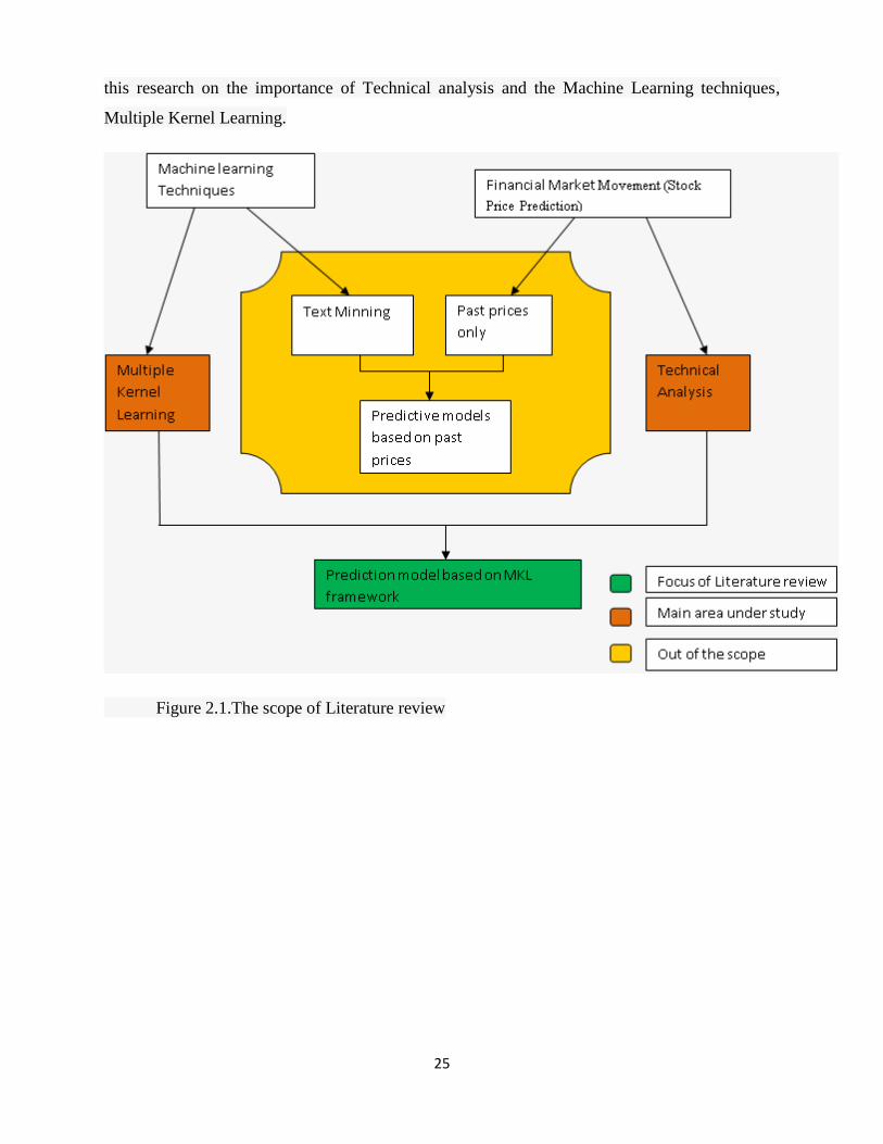
25
this research on the importance of Technical analysis and the Machine Learning techniques,
Multiple Kernel Learning.
Figure 2.1.The scope of Literature review

26
Chapter 3
Problem Statement
3.1 Problem Definition Unstable and assumptive aspects of the securities make it hard to predict the next day stock
prices The purpose of this research work is to predict the direction of stock prices going high or
low in future by the optimal combinations of different sub-kernels in Multiple Kernel Learning
Framework
3.2 Proposed Methodology
We propose a combination of different base kernels to predict the direction of stock prices going
up or down in future, which comprises a 2-tier framework.
• In first tier, we prepare the data and compute some technical indicators and normalize a
data set into a MKL data representation.
In second tier, design a model which has three sub-tasks : Construct different base kernels on the extracted featured set.
For the different base kernels, the weights are first learned and then tuned, and then these base
kernels are combined.
Performing Multiple kernel Learning through walk forward approach and predict the movement
of daily stock prices going up or down
This model is then used to predict stock direction. We make two kinds of predictions for
direction of stock prices: Predicting Daily Stock direction and Predicting a future trend.
Figure3.1 represents the diagram of our proposed model; it is made up of 3 components.
1) Preprocessing component
2) Prediction component
3) Performance component

27
Technical Indicator
Preprocessing component In preprocessing component, firstly we collected the raw data from the market and processed it
and then extracted some technical features or indicators based on the historical stock prices and
trading volume and then we finally normalized the whole features set.
Prediction component In prediction component , first we built different base kernels(RBF and Polykernel)on
normalized data set and then combined these base kernels through Multiple Kernel Learning
Framework , we then predicted the movement of daily’s stock trend such as up and down for the
next trading day from the previous day.
Performance Component In performance component, we computed some prediction measures such as Prediction
accuracy, F1-score, Harmonic Accuracy and Uncertainty score to evaluate the performance of
proposed and baseline methods.
Performance Component
Prediction Component
Multiple Kernel
Learning
Frameworks
Compute
Evaluation metrics
Web
Historical
Prices
Historical
volumes
Time Series
Data
TI-1
TI -2
TI -3
TI -4
TI -5
TI -6
TI -7
Preprocessing Component
Figure 3.1: Proposed Model

28
Chapter 4
Experimental Setup
The details of experimental design are given in this chapter. Figure 4.1 gives the overview of
methodology used.
4.1 System Requirements:
Hardware Processor Intel i3, Ram 4 +GB, Storage 160 GB, Frequency 2.93 GHz.
Operating System Ubuntu 12.04 LTS 32 bit.
Programming Language Implementation is in python language
IDE Programming is done in Eclipse IDE environment.
SHOGUN Toolbox API for machine learning tool version 3.2.0.
4.2 Data Collection and Data preprocessing
Data Collection
Data Pre-processing
Model Estimation/Training
Prediction
Results Analysis
Figure4.1: Methodology

29
The data set for our thesis have been provided by AlgoAnalytics Financial Consultancy Pvt
Ltd[23] it is proprietary data set comprising of three different stock from commodity market the
data set are namely FDATA and NDATA .Table1 give description about each data set some info
about used dataset.
Data set Number of rows
FData 1740
NData 2610
Table 4.1 Experimental Data
From the historical quotes of the data, compute some technical indicators based on it. The
preprocessing needed on the data for MKL framework and SVM was the normalization in the
range of [0,1]. Each of these dataset were then partitioned into two sets shown in the Figure 4.2
Historical data is used for model estimation/training, and then latest data was used for the
prediction performance. To use historical or latest data for MKL and SVM, it needed to be
further processed to convert it into the form of vector sets. For both MKL and SVM, the data
needs to be in the format of set of input-output vector. i.e. each vector contains the input for the
model and the output that the model should produce. This is the basic requirement of supervised
learning.
Latest index value Oldest index value
Latest Data (L) for
Testing
Historical Data (H) for
Training
Time
Total Data Latest index value Oldest index value
Figure 4.2: Data Partition

30
4.3Model Estimation/Training:
After pre-processing of historical data, used it to train the model for MKL and SVM. We did
many experiments to choose best kernel for stock data. We first choose linear kernel, sigmoid
kernel, Radial basis function kernel and Poly kernel. But we found that linear and sigmoid
kernels were not giving good results. . So we didn't investigate linear and sigmoid kernels
further. Then we used various combinations of Rbf kernel to find some best combinations. And
then we find out the combinations of Poly kernels. And after that we combined all these kernels
to get mix kernel methods. In which we used 11 kernels, out of which 8 were RBF kernels and
remaining 3 were poly kernels. We found a good result on our dataset. And then we learned
hyper parameters of these kernels from grid search. Then we fed it in MKL method in SHOGUN
toolbox. There is one more parameter on which performance of MKL method is dependent i.e.
Norms. We tried several norms with MKL kernels with walk forward approach with different
L: Latest Data
H : Historical Data
TVi: i th Training / testing
vector
W: Window size
n: Length of historical/latest
data
↑: Target output
TV1 W
W
TV2
W
TV3
W
TV(n-w)
W
TV(n-w+1)
Figure 4.3 Preparation of Vector sets for MKL and SVM

31
window sizes. And then we noticed the individual effect on the performance of both and their
combined effect on our datasets. Table4.2 shows the methods which we used in our experiments.
Methods Definition
MKL-1 Used 5 RBF kernels with sigma .25, .5, 1, 2, 4
MKL-2 Used 5 RBF kernels with sigma 2.5, 5, 10, 20,
40
MKL-3 Used 10 kernels in which 7 are RBF kernel
with sigma .25,2.5,1,4,10,16,20 and 3 are poly
kernels of degree 1,3,5.
MKL-4 Used 3 polykernel with degree 1,2,3
MKL-5 Used 3 polykernel with degree 1,2,3,4,5
SVM Support vector machine with C=1
Table 4.2 Details of each method.
In all of these methods SVM is the baseline method, MKL-3 is our proposed method which is
known as mix kernel approach and rest all are experimental method.
After learning the hyper parameters of MKL-3, train the model with walk forward approach and
evaluate its performance and compare with baseline method. Below discuss the walk forward
approach.
Walk Forward method for training and testing
We Used walk forward method for training and testing since underlying dynamics might change
rapidly in stock markets. In Walk Forward method, we made a window of k rows, first we
trained on k rows and then predicted (k+1)th day stock price. It will show movement (up and
down) from kth day stock price.. Now, we moved the window 1 row ahead, we have taken the k
rows again and trained again. Figure4.4 represents the walk forward approach. In our
experiment, for walk forward method we have used a window of three sizes: 400, 700 and 1000
training rows, for each window size we performed different MKL combination and computed
their performance at different norms.

32
In figure 4.4 N is the size of the training window, M is the size of testing data before window
moves forward.
4.4 Evaluation metrics
Confusion Matrix:
The columns of the confusion matrix represent the pre-dictions, and the rows represent the actual
class. Correct predictions always lie on the diagonal of the matrix. True Positive(TP)-True
Positives (TP) indicate the number of instances of the minor-ity that were correctly predicted
False Positive(FP)-Indicate the number of instances of the majority that were incorrectly
predicted as minority class instances
True Negative(TN)- Indicate the number of instances of the majority that were correctly
predicted.
False Negative(FN)- Indicate the number of the minority that were incorrectly predicted as
majority class instances
Though the confusion matrix gives a better outlook on how the classifier performed than
accuracy, a more detailed analysis is preferable which are provided by the further metrics .
Figure 4.5 shows the general structure of confusion matrix.
N M
N+2M M
N+M M
N+3M M
Figure 4.4 Walk Forward Method.

33
Other measures used to evaluate the classifier:
Prediction Accuracy
F1-Score =
Harmonic score =
Figure 4.5 Confusion Matrix
34
Chapter 5
Results and Analysis
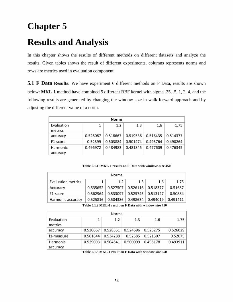
In this chapter shows the results of different methods on different datasets and analyze the
results. Given tables shows the result of different experiments, columns represents norms and
rows are metrics used in evaluation component.
5.1 F Data Results: We have experiment 6 different methods on F Data, results are shown
below: MKL-1 method have combined 5 different RBF kernel with sigma .25, .5, 1, 2, 4, and the
following results are generated by changing the window size in walk forward approach and by
adjusting the different value of a norm.
Table 5.1.1: MKL-1 results on F Data with windows size 450
Table 5.1.2 MKL-1 result on F Data with window size 750
Norms
Evaluation metrics
1 1.2 1.3 1.6 1.75
accuracy 0.530667 0.528551 0.524696 0.525275 0.526029
f1-measure 0.561644 0.534288 0.52585 0.521307 0.52075
Harmonic accuracy
0.529093 0.504541 0.500099 0.495178 0.493911
Table 5.1.3 MKL-1 result on F Data with window size 950
Norms
Evaluation metrics
1 1.2 1.3 1.6 1.75
accuracy 0.526087 0.518667 0.519536 0.516435 0.514377
F1-score 0.52399 0.503884 0.501474 0.493764 0.490264
Harmonic accuracy
0.496972 0.484983 0.481845 0.477609 0.476345
Norms
Evaluation metrics 1 1.2 1.3 1.6 1.75
Accuracy 0.535652 0.527507 0.526116 0.518377 0.51687
F1-score 0.562964 0.533097 0.525745 0.513127 0.50884
Harmonic accuracy 0.525816 0.504386 0.498634 0.494019 0.491411

35
MKL-2 have combined 5 different RBF kernel with sigma 2.5, 5, 10, 20, 40 and the following
results are generated by changing the window size in walk forward approach and by adjusting
the different values of a norm.
Norms
Evaluation metrics
1 1.2 1.3 1.6 1.75
accuracy 0.547507 0.546464 0.545478 0.538609 0.536
f1-measure 0.365432 0.364486 0.363208 0.353242 0.350272
Harmonic accuracy
0.315472 0.315991 0.316095 0.315758 0.316432
Table 1.1.4 MKl-2 results on F Data with window size 450
Norms
Evaluation metrics
1 1.2 1.3 1.6 1.75
accuracy 0.539217 0.540087 0.54058 0.537623 0.533797
f1-measure 0.297929 0.300674 0.303848 0.312117 0.31353
Harmonic accuracy
0.260164 0.261573 0.263979 0.276555 0.283505
Table 5.1.5 MKL-2 result on F Data with window size 750
Norms
Evaluation metrics
1 1.2 1.3 1.6 1.75
accuracy 0.549536 0.549101 0.547072 0.539275 0.537652
f1-measure 0.30574 0.306031 0.307112 0.314664 0.328124
Harmonic accuracy
0.252154 0.253127 0.25736 0.276643 0.292303
Table 5.1.6.MKL-2 results on F Data with window size 950
MKL-3 method have combined 11 different kernels in which 7 kernels are of RBF with sigma
.25,2.5,1,4,10,16,20 and the following results are generated by changing the window size in walk
forward approach and by adjusting the different values of a norm
Norms
Evaluation metrics
1 1.2 1.3 1.6 1.75
accuracy 0.528551 0.547159 0.548957 0.546116 0.544493
f1-measure 0.529383 0.510879 0.504853 0.486573 0.48202
Harmonic accuracy
0.499796 0.462451 0.454394 0.43916 0.436439
Table 5.1.7 MKL-3 results on F Data with window size 450

36
Norms
Evaluation metrics
1 1.2 1.3 1.6 1.75
accuracy 0.536319 0.547304 0.546696 0.539333 0.534986
f1-measure 0.5685 0.520125 0.510348 0.490462 0.481531
Harmonic accuracy
0.530644 0.471608 0.46242 0.450606 0.446563
Table 5.1.8 MKL-3 results on F Data with window size 750
Norms
Evaluation metrics
1 1.2 1.3 1.6 1.75
accuracy 0.530841 0.551478 0.552783 0.545594 0.544203
f1-measure 0.575393 0.533607 0.526034 0.508727 0.507902
Harmonic accuracy
0.542302 0.480818 0.471712 0.461988 0.462667
Table 5.1.9 MKL-3 results on F Data with window size 950
MKL-4 results method have combined 3 Poly kernels with degree (1,2, 3) and the following
results are generated by changing the window size in walk forward approach and by adjusting
the different values of a norm
Norms
Evaluation metrics
1 1.2 1.3 1.6 1.75
accuracy 0.531971 0.536029 0.536116 0.537217 0.537797
f1-measure 0.538169 0.532765 0.530454 0.526709 0.525896
Harmonic accuracy
0.50503 0.495782 0.493424 0.488634 0.487248
Table 5.1.10 MKL-4 results on F Data with window size 450
Norms
Evaluation metrics 1 1.2 1.3 1.6 1.75
accuracy 0.533362 0.534493 0.533768 0.531072 0.530957
f1-measure 0.540514 0.53265 0.5287 0.520311 0.518507
Harmonic accuracy
0.505981 0.497186 0.494033 0.488524 0.486886
Table 5.1.11. MKL-4 results on F Data with window size 750

37
Table 5.1.12. MKL-4 results on F Data with window size 950
MKL-5 method have combined 3 Polykernels with degree (1,2, 3,4,5) and the following results
are generated by changing the window size in walk forward approach and by adjusting the
different values of a norm.
Norms
Evaluation metrics
1 1.2 1.3 1.6 1.75
accuracy 0.534638 0.530551 0.529304 0.53342 0.534696
f1-measure 0.503602 0.501447 0.501029 0.507993 0.509218
Harmonic accuracy
0.468574 0.470716 0.471594 0.474135 0.474018
Table 5.1.13. MKL-5 results on F Data with window size 450
Table 5.1.14 MKL-5 results on F Data with window size 750
Table 5.1.15 MKL-5 results on F Data window size 950
SVM with C=1, getting results by changing the window size in walk forward approach.
Norms
Evaluation metrics
1 1.2 1.3 1.6 1.75
accuracy 0.539188 0.538116 0.538261 0.538174 0.538609
f1-measure 0.573574 0.570474 0.569343 0.565562 0.564797
Harmonic accuracy
0.533024 0.530942 0.529692 0.526039 0.524877
Norms
Evaluation metrics
1 1.2 1.3 1.6 1.75
accuracy 0.536377 0.527043 0.524928 0.522609 0.523101
f1-score 0.505457 0.501451 0.499908 0.498141 0.499802
Harmonic accuracy
0.468574 0.474312 0.474972 0.475615 0.476709
Norms
Evaluation metrics
1 1.2 1.3 1.6 1.75
accuracy 0.549478 0.546377 0.543768 0.537623 0.53513
f1-score 0.52265 0.523331 0.5219 0.520327 0.520022
Harmonic accuracy
0.471831 0.47582 0.47713 0.48193 0.484167
38
Evaluation metrics
Window Size
Accuracy f1-score Harmonic accuracy
Uncertainty Score
ws=450 0.522754 0.392637 0.374645 0.509506
ws=750 0.507101 0.372579 0.374516 0.50337
ws=950 0.50371 0.366696 0.373077 0.502187
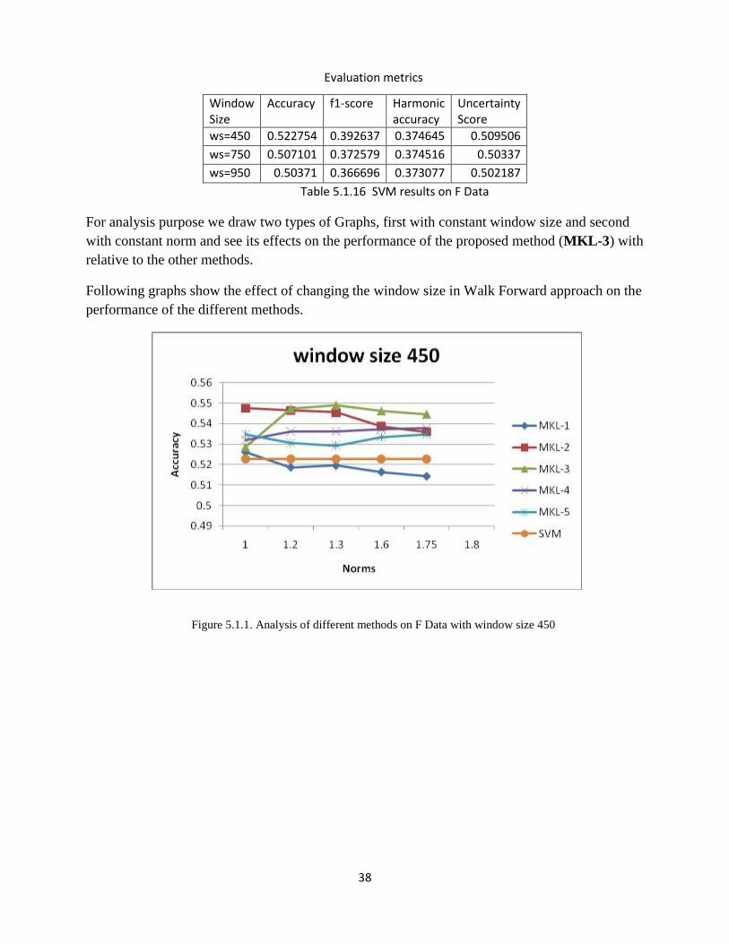
Table 5.1.16 SVM results on F Data
For analysis purpose we draw two types of Graphs, first with constant window size and second
with constant norm and see its effects on the performance of the proposed method (MKL-3) with
relative to the other methods.
Following graphs show the effect of changing the window size in Walk Forward approach on the
performance of the different methods.
Figure 5.1.1. Analysis of different methods on F Data with window size 450

39
In above figures 5.1.1,5.1.2 & 5.1.3 our proposed method MKL-3 performs better than other
methods with different window sizes. For window size 450 MKl-3 perform good at norm 1.3, for
window size 750 MKL-3 perfrom good at 1.2 and 1.3 norms and for window size 950 MKL-3
performs better for all norms. Next, we show the graphs with constant norms , x-axis represent
different window size and y-axis represent Prediction Accuracy.
Figure5.1.3. Analysis of different methods on F Data with window size 950
Figure5.1.2. Analysis of different methods on F Data with window size 750

40
Figure5.1.4. Analysis of different methods on F Data at Norm 1
Figure 5.1.5. Analysis of different methods on F Data at Norm 1.2

41
Figure 5.1.6. Analysis of different methods on F Data at Norm 1.3
Figure 5.1.7 Analysis of different methods on F Data at Norm 1.6
42
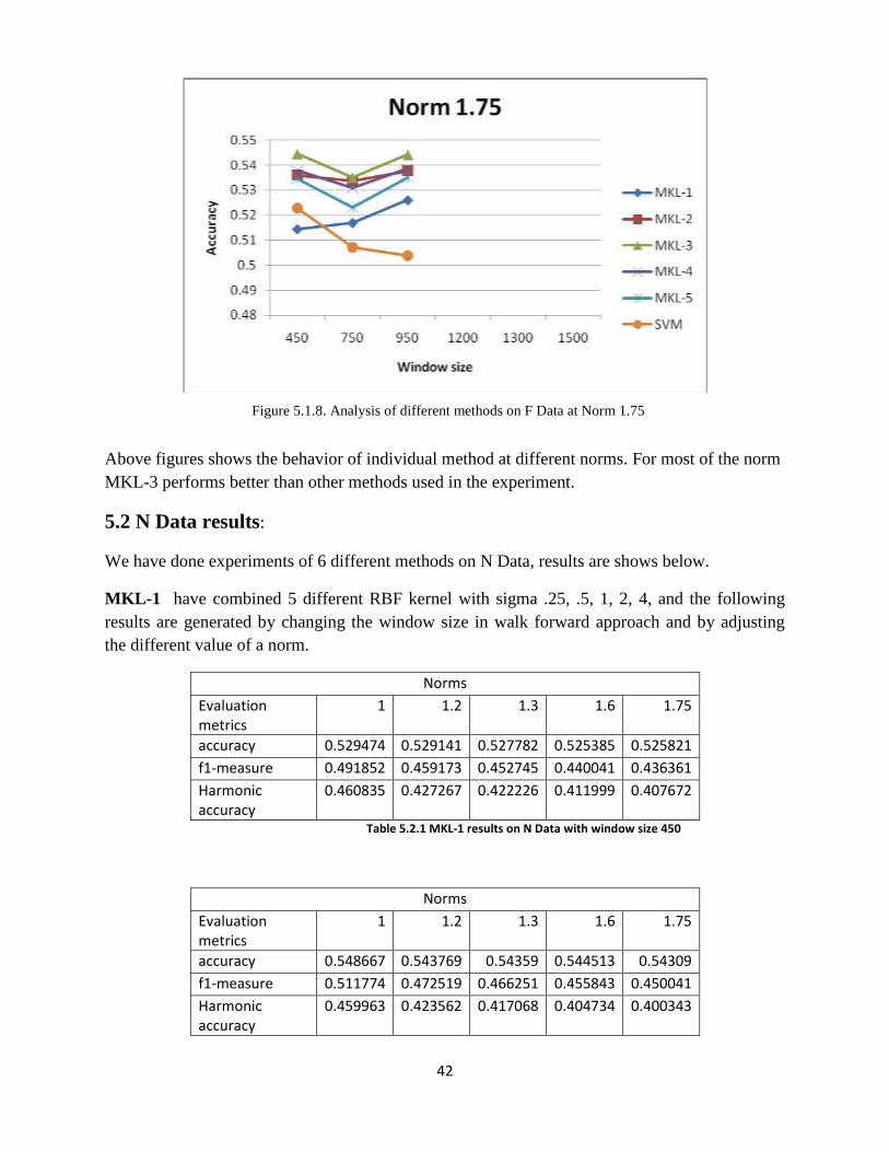
Above figures shows the behavior of individual method at different norms. For most of the norm
MKL-3 performs better than other methods used in the experiment.
5.2 N Data results:
We have done experiments of 6 different methods on N Data, results are shows below.
MKL-1 have combined 5 different RBF kernel with sigma .25, .5, 1, 2, 4, and the following
results are generated by changing the window size in walk forward approach and by adjusting
the different value of a norm.
Norms
Evaluation metrics
1 1.2 1.3 1.6 1.75
accuracy 0.529474 0.529141 0.527782 0.525385 0.525821
f1-measure 0.491852 0.459173 0.452745 0.440041 0.436361
Harmonic accuracy
0.460835 0.427267 0.422226 0.411999 0.407672
Table 5.2.1 MKL-1 results on N Data with window size 450
Norms
Evaluation metrics
1 1.2 1.3 1.6 1.75
accuracy 0.548667 0.543769 0.54359 0.544513 0.54309
f1-measure 0.511774 0.472519 0.466251 0.455843 0.450041
Harmonic accuracy
0.459963 0.423562 0.417068 0.404734 0.400343
Figure 5.1.8. Analysis of different methods on F Data at Norm 1.75

43
Table 5.2.2. MKL-1 results on N Data with window size 750
Norms
Evaluation metrics
1 1.2 1.3 1.6 1.75
accuracy 0.554474 0.549462 0.549013 0.545885 0.544333
f1-measure 0.513802 0.479886 0.473375 0.458783 0.452341
Harmonic accuracy
0.455293 0.424415 0.417916 0.406136 0.401205
Table 5.2.3 MKL-1 results on N Data with window size 950
MKL-2 have combined 5 different RBF kernel with sigma 2.5, 5, 10, 20, 40 and the following
results are generated by changing the window size in walk forward approach and by adjusting
the different values of a norm.
Norms
Evaluation metrics
1 1.2 1.3 1.6 1.75
accuracy 0.541769 0.548462 0.549923 0.548231 0.548756
f1-measure 0.548883 0.541251 0.541745 0.53711 0.536229
Harmonic accuracy
0.507532 0.49213 0.491053 0.4879 0.486362
Table 5.2.4 MKL-2 results on N Data with window size 450
Norms
Evaluation metrics
1 1.2 1.3 1.6 1.75
accuracy 0.55309 0.557654 0.556064 0.553744 0.553641
f1-measure 0.549235 0.545648 0.543799 0.542842 0.542773
Harmonic accuracy
0.495721 0.486666 0.486428 0.487992 0.488032
Table 5.2.5. MKL-2 results on N Data with window size 750
Norms
Evaluation metrics
1 1.2 1.3 1.6 1.75
accuracy 0.543321 0.546 0.548282 0.554974 0.5535
f1-measure 0.535623 0.531686 0.530951 0.538097 0.537594
Harmonic accuracy
0.491696 0.484521 0.481176 0.481392 0.482518
Table 5.2.6. MKL-2 results on N Data with window size 950
MKL-3 method have combined 11 different kernels in which 7 kernels are of RBF with sigma
.25,2.5,1,4,10,16,20 and 3 kernels are of Poly kernel with degree 1,3,5 the following results are

44
generated by changing the window size in walk forward approach and by adjusting the different
values of a norm.
Norms
Evaluation metrics
1 1.2 1.3 1.6 1.75
accuracy 0.549436 0.560987 0.561295 0.559731 0.558872
f1-measure 0.57532 0.568896 0.566612 0.55925 0.556724
Harmonic accuracy
0.528035 0.50875 0.505867 0.499406 0.497558
Uncertainty score
0.525135 0.532164 0.532357 0.531403 0.530879
Table 5.2.7 MKL-3 results on N Data with window size 450
Norms
Evaluation metrics
1 1.2 1.3 1.6 1.75
accuracy 0.557462 0.563756 0.563705 0.564051 0.563077
f1-measure 0.579602 0.568191 0.565804 0.563122 0.561379
Harmonic accuracy
0.524408 0.504911 0.502292 0.498896 0.498039
Table5.2.8 MKL-3 results on N Data with window size 750
Norms
Evaluation metrics
1 1.2 1.3 1.6 1.75
accuracy 0.560846 0.561333 0.564103 0.566667 0.567513
f1-measure 0.574696 0.565202 0.566824 0.567332 0.567734
Harmonic accuracy
0.515363 0.504253 0.502993 0.500691 0.50019
Table 5.2.9 MKL-3 results on N Data with window size 950
MKL-4 method have combined 3 Poly kernels with degree (1,2, 3) and the following results are
generated by changing the window size in walk forward approach and by adjusting the different
values of a norm
Norms
Evaluation metrics
1 1.2 1.3 1.6 1.75
accuracy 0.524526 0.532603 0.532756 0.536615 0.537321
f1-measure 0.507025 0.512144 0.50997 0.510058 0.5096
Harmonic accuracy
0.481939 0.478533 0.476089 0.471911 0.470639
Table 5.2.10MKL-4 results on N Data with window size 450

45
Norms
Evaluation metrics
1 1.2 1.3 1.6 1.75
accuracy 0.523692 0.529487 0.532244 0.531564 0.528897
f1-measure 0.476791 0.481008 0.48461 0.483824 0.481677
Harmonic accuracy
0.451783 0.449549 0.450136 0.450098 0.450919
Table 5.2.11 MKL-4 results on N Data with window size 750
Norms
Evaluation metrics
1 1.2 1.3 1.6 1.75
accuracy 0.519577 0.521718 0.523769 0.523795 0.522923
f1-measure 0.476934 0.47598 0.478755 0.479513 0.478488
Harmonic accuracy
0.45653 0.453171 0.453713 0.454463 0.454388
Table 5.2.12 MKL-4 results on N Data with window size 950
MKL-5 have combined 3 Poly kernels with degree (1,2, 3,4,5) and the following results are
generated by changing the window size in walk forward approach and by adjusting the different
values of a norm
Norms
Evaluation metrics
1 1.2 1.3 1.6 1.75
accuracy 0.552218 0.552308 0.551154 0.549551 0.549654
f1-measure 0.551188 0.545514 0.542137 0.536398 0.535449 Table 5.2.13 MKL-5 results on N Data with window size 450
Norms
Evaluation metrics
1 1.2 1.3 1.6 1.75
accuracy 0.549756 0.554654 0.555026 0.553769 0.55241
f1-measure 0.550661 0.552422 0.551286 0.544853 0.541042
Harmonic accuracy
0.500922 0.497488 0.49583 0.490167 0.487518
Table 5.2.14 MKL-5 results on N Data with window size 750

46
Norms
Evaluation metrics
1 1.2 1.3 1.6 1.75
accuracy 0.543551 0.545987 0.545833 0.546179 0.545577
f1-measure 0.542337 0.544603 0.543133 0.537728 0.535336
Harmonic accuracy
0.498638 0.498449 0.497032 0.490832 0.488918
Table 5.2.15MKL-5 results on N Data with window size 950
SVM with C=1, getting results by changing the size of window in walk forward approach
Evaluation metrics window size accuracy f1-score Harmonic accuracy
ws=450 0.514397 0.357222 0.341644
ws=750 0.510949 0.211631 0.200617
ws=950 0.509808 0.187406 0.178282 Table: 5.2.16 SVM Results on NData
Following graphs shows the effect of changing the window size in Walk Forward approach on
the performance of the different methods.
Figure 5.2.1 Analysis of different methods on N Data with window size 450

47
Figure 5.2.2 Analysis of different methods on N Data with window size 750
Figure 5.2.3 Analysis of different methods on N Data with window size 950
In above figures 5.2.1, 5.2.2 & 5.2.3 our proposed method MKL-3 performs better than other
methods for all norms with different window sizes
Next, we show the graphs with constant norms, x-axis represents different window size and y-
axis represents Prediction Accuracy

48
Figure 5.2.4 Analysis of different methods on N Data at Norm 1
Figure 5.2.5 Analysis of different methods on N Data at Norm 1.2
49
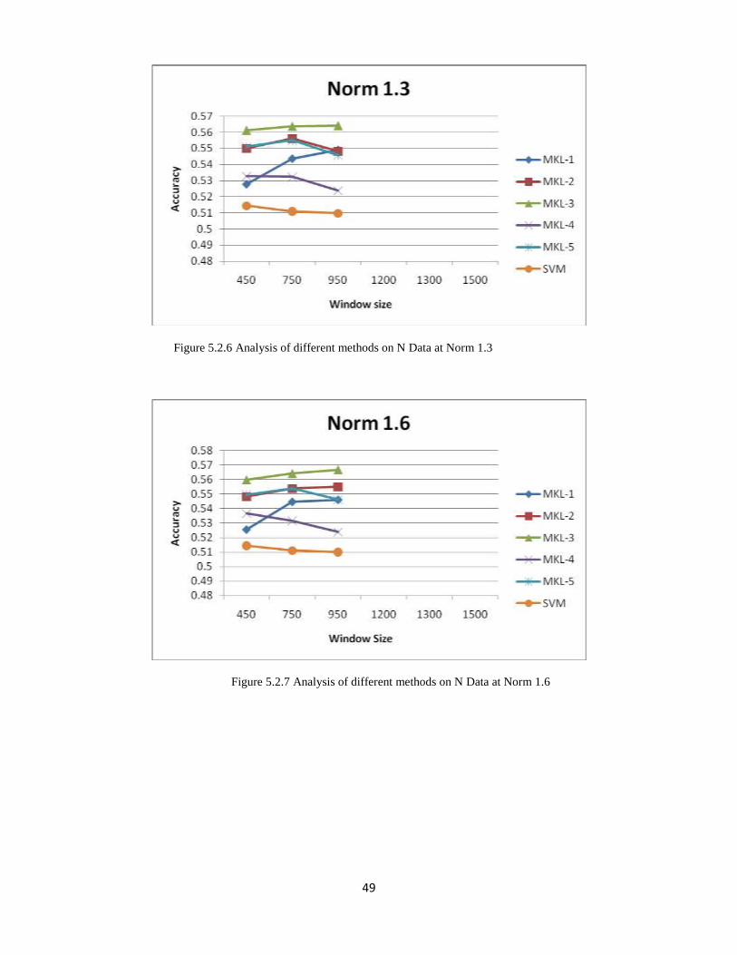
Figure 5.2.6 Analysis of different methods on N Data at Norm 1.3
Figure 5.2.7 Analysis of different methods on N Data at Norm 1.6
50
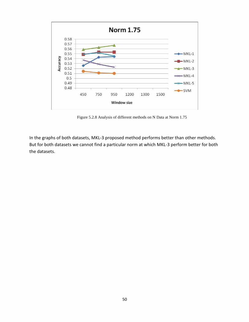
Figure 5.2.8 Analysis of different methods on N Data at Norm 1.75
In the graphs of both datasets, MKL-3 proposed method performs better than other methods.
But for both datasets we cannot find a particular norm at which MKL-3 perform better for both
the datasets.

51
Chapter 6
Conclusion & Future Work
Stock Market is difficult to predict precisely because the financial abstract has certain non
stationery characteristics or properties which make it difficult to predict. In this project, we have
learned and tuned the weights using several combination of kernels. In Algorithm proposed
solution of mix kernel we have combined 11 kernels. Out of which 8 were RBF kernels and
remaining 3 were polynomial kernels. Now, one more parameter can be changed i.e. norms.We
have tried 5 to 7 different norms and 3 different window sizes. According to our result,
worldwide there is no norm that behave accurately for all securities. If a particular norm is better
for a particular security, it is not important that it will work better for other securities too. So, it is
difficult to find a particular norm or model that behave accurately for all securities in stocks.
And our model ' Mix Kernel is showing better behaviour than other baseline methods in our
experiments. For the monetary analyst, individual and for people who invest in corporate , it will
be very useful. We can easily forecast the stock market movement with such miniature and by
taking some appropriate action, maximum profit can be gained.
This chapter throws light on the future enhancements that can be carried out. Some of the further
enhancements would be to implement the approach for parallel computing platform for training
MKL which would help reduce the time required for the approach.

52
References [1] R.S. Tsay. Analysis of Financial Time Series. Wiley 2002, Financial Engineering
[2] Wikipedia. Algorithmic Trading. http://en.wikipedia.org/wiki/Algorithmic trading, April2012
[3] C.Burges. A tutorial on support vector machines for pattern recognition. Data Mining and
Knowledge discovery, 1998
[4] J.Murphy , Technical analysis of the financial markets, Prentice Hall, London, 1998.
[5] C.J. Neely, Technical analysis and the profitability of U.S. foreign exchange intervention
1998.
[6] V.Vapnik, The Nature of Statistical Learning Theory, Springer-Verlag,1999
[7] M. Kolft, U.Brefeld, P.Laskov, and S. Sonnenburg. “Non-sparse multiple kernel learning ,
Automatic selection of optimal kernels”, 2008.
[9] A.S. Weigend, S. Shi. “Predicting daily probability distributions of S&P500 returns. Journal
of Forecasting”, 2000
[10] M.R. Hassan, B. Nath, M. Kirley “A fusion model of HMM, ANN and GA for stock market
forecasting”. Journal of Machine learning 33 , 2007
[11] M.R. Hassan, B. Nat .“ A combination of hidden Markov model and fuzzy model for stock
market forecasting” Journal of Neurocomputing 72, 2009
[12] B. Dhingra, A. Gupta. “Stock Market Prediction Using Hidden Markov Models”. IEEE
Student chapter conference on systems and engineering, MNNIT Allahabad, March 16-18, 2012,
Allahabad.
[13]R.S. Tsay. Analysis of Financial Time Series. Wiley 2002, Financial Engineering
[14] W. Brock, J. Lakonishok, and B. Lebaron, “Simple technical trading rulesand the stochastic
properties of stock returns,” Wisconsin Madison – Social Systems, 1991.
[15] Y.-H. Lui and D. Mole, “The use of fundamental and technical analyses by foreign
exchange dealers: Hong kong evidence,” Journal of International Money and Finance, june 1999
[16] B. LeBaron, “Technical trading rule profitability and foreign exchange intervention
”National Bureau of Economic Research, Mar. 1996.
[17] A. W. Lo, H. Mamaysky, and J. Wang, “Foundations of technical analysis:Computational
algorithms, statistical inference, and empirical implementation,” National Bureau of Economic
Research, Inc, NBER Working Papers , 2000.

53
[18] On the profitability of technical trading rules based on artificial neural networks:: Evidence
from the Madrid stock market,” Economics Lettersvol. 69, 2000.
[19] C. J. Neely and P. A. Weller, “Intraday technical trading in the foreign exchange market,”
Federal Reserve Bank of St. Louis.
[20] K. A. Kavajecz, “Technical analysis and liquidity provision,” Review of Financial Studies,
vol. 17, 2004.
[21]Wei Cheng, Lorry Wagner, and Chien-Hua Lin “Financial forecasting with a system of
neural networks”.
[22]Chi-Cheong ,Chris Wong, Man-Chung Lam. “Financial time series forecasting by neural
networks using conjugate gradient learning algorithm and multiple linear Regression weight
initialization”.
[23] Lijuan Cao and Francis E.H Tay. “Finacial forecasting using support vector machine”
Neural Computing & Applications, May 2001.
[24] M.R. Hassan, B. Nath, M. Kirley. “A fusion model of HMM, ANN and GA for stock
market forecasting” , IEEE conference on systems and engineering.
[25]M.R. Hassan.”A combination of hidden Markov model and fuzzy model for stock market
forecasting”Journal of Neurocomputing 72, 2009
[26] B. Dhingra, A. Gupta. “Stock Market Prediction Using Hidden Markov Models”. IEEE
Student chapter conference on systems and engineering.