multiple feature temporal models.. · the choice of color space may result in some kind of...

Chapter 2

Semantics from low-level features

Objects, background and other elements that form a scene have their own character-istic low-level features. A person standing in front of a camera will be the cause ofcertain colors and textures that appear in the image sequence that is being created. Ifthat person walks, a certain motion pattern will be observed as well. Image featurescarry information that characterizes the semantic concepts that caused them. Thischapter explores the semantic information that is implicitly contained in low-levelfeatures. This information can be used for video indexing and annotation, and alsoto obtain intermediate-level semantic descriptions of contents to be used for higherlevel video structure analysis. Color and motion are two main low-level featuresthat can be used for these purposes. First, the use of color as a semantic carrieris reviewed. Then, the semantics that can be inferred from motion information isanalyzed in the domain of news videos. Finally, different ways of combining multiplefeatures for the characterization of semantic concepts are reviewed as well.

2.1 Semantics from color

Color has been used as the simplest way to do object recognition and retrievalsince the introduction of color histogramming techniques for video indexingby Swain and Ballard in [69]. A color histogram summarizes the colors of

an object. Therefore, certain information about the appearance of an object andits identity is contained in it. A color histogram can thus be seen as a kind ofintermediate-level semantic representation of an object.

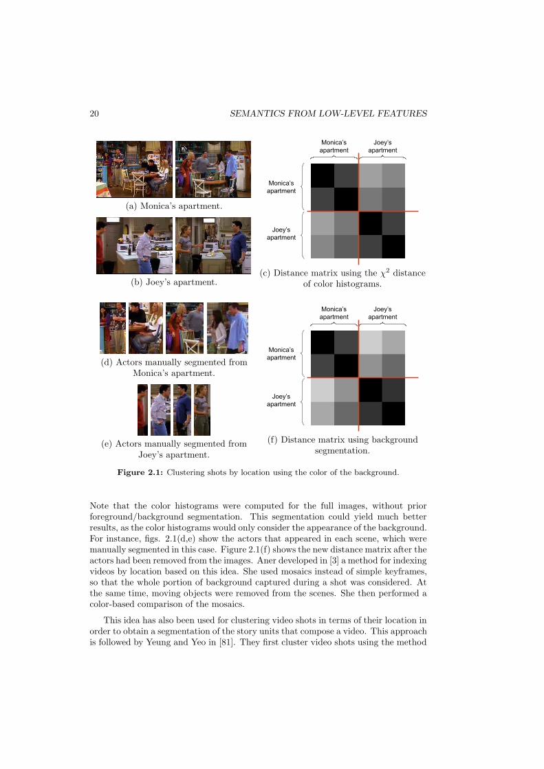
When the object that is characterized using color turns out to be the backgroundof the scene, a characterization of the location is obtained. For example, the images infig. 2.1(a,b) were shot at two different locations from the sitcom Friends: Monica’s andJoey’s apartments. Color histograms and the χ2 distance were used to compute thedistance matrix shown in fig. 2.1(c), where the two clusters can be clearly noticed.

19

20 SEMANTICS FROM LOW-LEVEL FEATURES

(a) Monica’s apartment.

(b) Joey’s apartment.

Monica’s

apartment

Monica’s

apartment

Joey’s

apartment

Joey’s

apartment

(c) Distance matrix using the χ2 distanceof color histograms.

(d) Actors manually segmented fromMonica’s apartment.

(e) Actors manually segmented fromJoey’s apartment.

Monica’s

apartment

Monica’s

apartment

Joey’s

apartment

Joey’s

apartment

(f) Distance matrix using backgroundsegmentation.

Figure 2.1: Clustering shots by location using the color of the background.

Note that the color histograms were computed for the full images, without priorforeground/background segmentation. This segmentation could yield much betterresults, as the color histograms would only consider the appearance of the background.For instance, figs. 2.1(d,e) show the actors that appeared in each scene, which weremanually segmented in this case. Figure 2.1(f) shows the new distance matrix after theactors had been removed from the images. Aner developed in [3] a method for indexingvideos by location based on this idea. She used mosaics instead of simple keyframes,so that the whole portion of background captured during a shot was considered. Atthe same time, moving objects were removed from the scenes. She then performed acolor-based comparison of the mosaics.

This idea has also been used for clustering video shots in terms of their location inorder to obtain a segmentation of the story units that compose a video. This approachis followed by Yeung and Yeo in [81]. They first cluster video shots using the method

2.1. Semantics from color 21

Color Feelings evoked in the viewer

Red Happiness, dynamism, aggressiveness, violence, powerOrange Glory, solemnity, vanity, progressGolden yellow Richness, prosperity, happinessDark yellow Deception, cautionGreen Calm, relax, hopeBlue Gentleness, fairness, faithfulness, virtuePurple Melancholy, fearBrown Relax (mostly used as background color)

Table 2.1: Feelings related to colors, as considered by semiotics.

from [80], which is based on the RGB color histogram intersection distance. Higher-level knowledge about the production process in the domain of sitcoms is then usedto generate a Scene Transition Graph (STG). The main assumption is that repeatedshots of the same persons or same settings, alternating or interleaving with othershots, are often deployed in many programs to convey parallel events in a scene, suchas conversations and reactions. Temporal constraints are also applied, so that if twovisually similar shots occur far apart in the time line, they may potentially belongto different scenes. A similar approach is followed in [41] by Kender and Yeo. Theymeasure probable scene boundaries by calculating a short term memory-based modelof shot-to-shot coherence. The assumption that visually similar shots repeat in ascene and the temporal constraint are also considered.

A different point of view about the semantics conveyed by color is given froma semiotics perspective. Semiotics is concerned with unspoken messages that arecommunicated to the observer by the use of visual features. For instance, warm colorsgrab the attention of the viewer and convey dynamism. On the other hand, cold colorssuggest gentleness, calm, relax and faithfulness. Each color can be associated to aset of feelings, which are summarized in table 2.1. The use of saturated colors isconsidered a sign of unrealistic situations, giving a sense of fancy and joyful worlds,and thus communicates happiness. The presence of light colors also induces the viewerto feel calm and relax. All these observations can be used to organize a video archivein terms of complex semantic concepts.

Two main ways of improving the performance of color descriptions for objectrecognition and retrieval have been proposed and are reviewed next.

2.1.1 Invariant color representations

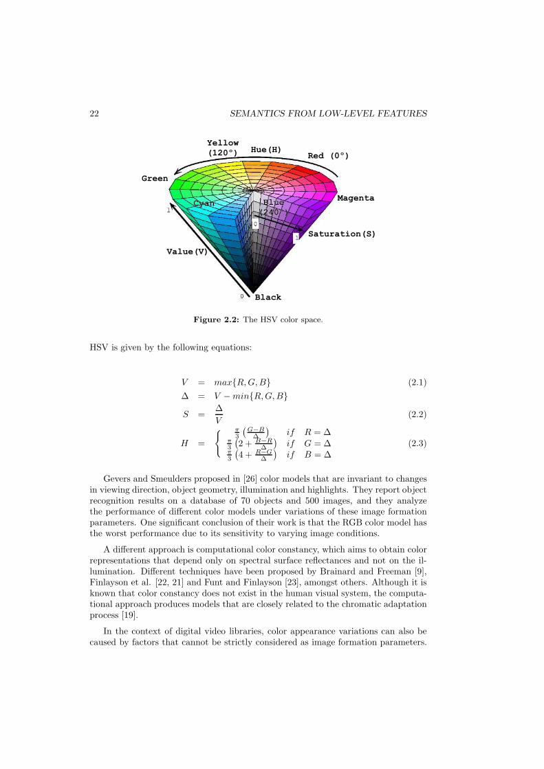
These works are concerned on obtaining color features that do not depend on somespecific image formation factors like lightning conditions. The choice of color spacemay result in some kind of invariance. For example, some authors prefer to use theHSV color space and drop the V component, which is directly related to luminance,instead of the RGB space, where the three components are affected by luminance.The HSV color space is depicted in fig. 2.2. The transformation from RGB values to


Red (0º)

Yellow

(120º)

Green

Cyan Blue

(240º)

Magenta

Black

Saturation(S)

Value(V)

Hue(H)

Figure 2.2: The HSV color space.

HSV is given by the following equations:

V = max{R, G, B} (2.1)

∆ = V − min{R, G, B}

S =∆

V(2.2)

H =

{ π3

(

G−B∆

)

if R = ∆π3

(

2 + B−R∆

)

if G = ∆π3

(

4 + R−G∆

)

if B = ∆(2.3)

Gevers and Smeulders proposed in [26] color models that are invariant to changesin viewing direction, object geometry, illumination and highlights. They report objectrecognition results on a database of 70 objects and 500 images, and they analyzethe performance of different color models under variations of these image formationparameters. One significant conclusion of their work is that the RGB color model hasthe worst performance due to its sensitivity to varying image conditions.

A different approach is computational color constancy, which aims to obtain colorrepresentations that depend only on spectral surface reflectances and not on the il-lumination. Different techniques have been proposed by Brainard and Freeman [9],Finlayson et al. [22, 21] and Funt and Finlayson [23], amongst others. Although it isknown that color constancy does not exist in the human visual system, the computa-tional approach produces models that are closely related to the chromatic adaptationprocess [19].

In the context of digital video libraries, color appearance variations can also becaused by factors that cannot be strictly considered as image formation parameters.

2.1. Semantics from color 23

DCP 1

DCP 2

DCP 3

DCP 4

DCP 5

PCS

DCP 2

DCP 3

DCP 4

DCP 5DCP 1

Figure 2.3: In general, for N device-dependent color profiles (DCP), we would needN(N − 1) color space transformations (left). The ICC defines a device-independentcolor space, called Profile Connection Space (PCS), so that only one transform perdevice is needed (right).

The most typical case is color appearance variations due to the use of different acqui-sition hardware, where the sensitivity of their sensors may vary. In this case, colorinvariants and color constancy algorithms may not be appropriate. A more suitableapproach for this kind of variations is finding mappings between device-dependentcolor spaces. The International Color Consortium (ICC) has made an effort to stan-dardize device-dependent color profiles [37]. This standard defines a Profile Con-nection Space (PCS), which is a device-independent color space, so that only onetransformation must be defined per input or output device. This scheme is depictedin fig. 2.3. The ICC work has been specifically oriented to desktop publishing ap-plications. Its application is arguable in the domain of digital video libraries, wherethe source of a video may be unknown, and the footage goes through several colortransformations caused by the VCR, the frame grabber, and other hardware that maybe involved in the digitization process.

Device-dependent color appearances can be characterized by the parameters ofa set of Gaussian distributions. In this way, the intrinsic appearance of a color isdetermined by the contribution of each Gaussian distribution to it. Mappings arethen defined between different device-dependent color spaces in order to keep theintrinsic appearance of colors, that is, their identities. A device-independent colorappearance space is also defined as a normalized representation of color identities. Inthis way, the ICC approach can be implemented, and only one mapping per devicemust be defined. They report experimental results on applications like skin colorsegmentation and image retrieval, and a comparison with color constancy approaches.Their experiments show that the grayworld color constancy algorithm provides asgood results as their method, but with a lower computational cost. However, colorappearances are not preserved using the grayworld approach, so that it cannot be usedfor the skin color segmentation application. Therefore, the conclusion is inverted: theGaussian mixture approach to color correction is appropriate for applications wherecolor appearance must be conserved, and its performance is high for image retrievalpurposes as well. The main disadvantage of this method is that a calibration pattern,like the ones in fig. A.5, has to be acquired using the hardware that is characterized,


and this may not always be possible. More details about the characterization of devicecolor spaces, and mappings between them are given in appendix A.

2.1.2 Enhanced color representations

Different extensions to color histograms have been developed. They are mainly con-cerned on including spatial information within the summarized color representationin order to capture the shape and distribution of the colors of the object or image.Color histograms lack spatial information, and this can cause images with very dif-ferent appearances to have very similar histograms. Color coherence vectors (CCV)were defined by Pass et al. in [62]. The CCV measures the spatial coherence of thepixels of a given color. If regions of a certain color in the image are large, then thatcolor has high coherence, and has low coherence otherwise. Huang et al. introducedthe color correlogram in [36]. They define the color correlogram as a table indexedby color pairs, where the k-th entry for < i, j > specifies the probability of finding apixel of color j at a distance k from a pixel of color i in the image. They conclude thatsuch an image feature is robust in tolerating large changes in appearance of the samescene caused by changes in viewpoint positions, changes in the background scene,partial occlusions and camera zoom that causes radical changes in shape. The defini-tion is basically the same as that of a cooccurrence matrix for the representation ofgraylevel spatial textures. Therefore, the color correlogram is a way of characterizinga statistical color texture.

2.2 Semantics from motion

Motion information analysis usually requires the segmentation of different movingobjects and background entities. This task is particularly challenging on its own andis matter of deep research [4]. On the other hand, motion patterns can be representedusing temporal motion textures. Temporal motion textures extend classical grayscaletexture analysis techniques. The idea is to characterize patterns of motion along time.These patterns, like in spatial textures, can be either statistical (windblown trees) orstructural (a person walking). In contrast, we find motion events, which are singleevents that do not repeat in space or time (opening a door).

Nelson and Polana showed in [54] that certain statistical spatial and temporalfeatures that can be derived from approximations to the motion field have invariantproperties, and can be used to classify regional activities such as windblown treesor chaotic fluid flow, that are characterized by complex, non-rigid motion. Theyused a set of statistical features computed on the normal flow field for each texturein order to characterize and classify the following textures: fluttering crepe paperbands, cloth waving in the wind, motion of tree in the wind, flow of water in ariver, turbulent motion of water, uniformly expanding image produced by forwardobserver motion, and uniformly rotating image produced by observer roll. Szummerand Picard modeled temporal textures in [70] using the spatio-temporal autoregressive

2.2. Semantics from motion 25

model (STAR), which expresses each pixel as a linear combination of surroundingpixels lagged both in space and in time. This model not only provides a base forrecognition, but also for synthesis of temporal textures.

A statistical characterization of a temporal motion texture will globally considermotion information from the whole scene, thus including global and object motionsin it. In this way, object/background segmentation is not required to represent themotion patterns in a video shot. A representation of temporal motion textures basedon their temporal cooccurrence matrices is presented next. This method captures theunderlying motions in the scene, as well as their temporal variations.

2.2.1 Temporal motion texture modeling

In the same way a spatial texture is regarded as a particular spatial distribution ofgray level values, a temporal motion texture can be seen as a distribution of spatio-temporal motion measures. Bouthemy and Fablet’s approach [8] is based on extendingthe well-known characterization of textures using cooccurrence matrices developed byHaralick in [35]. For a spatial texture, each value Pd(i, j) in the cooccurrence matrixPd contains the probability of finding the values i and j with a spatial distance d inthe texture. The extension to spatio-temporal motion distributions is straightforward,being Pd(i, j) the probability of finding motion observations i and j at a temporaldistance d, and in the same spatial position. We will consider the norm of the velocityvectors as our observations. These observations must be considered along a significantset of frames in order to correctly capture the temporal behavior of the texture. Thus,the temporal cooccurrence for the pair of motion observations (i, j) at the temporaldistance d in image sequence I(x, y, t), t ∈ [t1, t2] is defined as:

Pd(i, j) =#{(x, y, t) | vobs(x, y, t) = i, vobs(x, y, t + d) = j, t, (t + d) ∈ [t1, t2]}

#{(x, y, t) | t, (t + d) ∈ [t1, t2]}(2.4)

where vobs(x, y, t) is the motion observation in position (x, y) and time t.

A reduced set of statistical descriptors can then be obtained from a cooccurrencematrix in order to obtain a reduced and meaningful characterization of the underlyingtemporal texture. Bouthemy and Fablet report two sets of these descriptors:

1. Entropy, inverse difference moment, acceleration, kurtosis and difference kurto-sis.

2. Average, variance, Dirac, angular second moment (ASM) and contrast.

These descriptors are respectively defined in [17] and [8]. The second set hasthe advantage that each feature has an interpretation in terms of motion perception.The average is directly related to the amount of motion, whereas variance and Diracshow the degree of spreading of the motion distribution. The ASM measures the


temporal coherence of motion and contrast is related to the average acceleration.These descriptors are mathematically defined as:

• Average: A =∑

(i,j) iPd(i, j)

• Variance: σ2 =∑

(i,j)(i − A)2Pd(i, j)

• Dirac: δ = A2/σ2

• Angular Second Moment: ASM =∑

(i,j) Pd(i, j)2

• Contrast: Cont =∑

(i,j)(i − j)2Pd(i, j)

In order to compute the cooccurrence matrix, motion observations must be quan-tized. The norm of the velocity vectors at each spatial location is considered. Notethat the orientation component of velocity is dropped. Quantization is a delicatestep, as the dynamic range of motion observations has to be taken into account. Thisrange is domain-dependant, and in the case of news videos the maximum motionfound is commonly small. In this case, 16 quantization levels within the range [0,3]is a suitable value, so that cooccurrence matrices Pd will be sized 16 × 16.

It is important to note that the accuracy needed when computing velocity vectorfields is not necessarily high. Noise and computation errors at this level will not have asignificant effect on the final descriptors that will characterize a temporal texture. Weused an accurate algorithm for optical flow computation by Black and Anandan [6],which embeds previous common approaches within a robust estimation framework.This approach takes into account possible violations of the data conservation andspatial coherence constraints on image motion. These constraints are necessary tomake optical flow computation a well-posed problem, but can lead to estimationerrors when they are not completely fulfilled. However, tests performed using a simplecorrelation method for optical flow estimation show that the final descriptors obtainedare practically the same.

2.2.2 Semantic classification based on temporal motion tex-

ture

We have seen that the automatic detection of anchors in news videos plays a key rolein order to obtain their high-level semantic structure. Besides, special correspondentsand people relevant to the piece of news, i.e. politicians or other celebrities, aresignificant in the indexing and annotation senses. This section is focused on findingshots of individuals using motion information, considering that these shots appear asclose-ups and medium shots as they are defined by film-making terminology [28]. Thedifference between a close-up and a medium shot is basically defined by the distancefrom the camera to the subject matter. Considering a person shot, a close-up willshow mainly his/her face or head, while a medium shot would include head, chestand arms. Examples are shown in fig. 2.4.


Figure 2.4: Close-ups and medium shots containing individuals.

Peker et al. observed in [63] two main facts that can be used as heuristics fordetecting close-ups: low coherence of motion along time and relatively large motions.Both facts are due to the short distance between the camera and the object. Thefollowing observations on the motion-related descriptors obtained from our data setare common for close-up shots with significant motion:

• relatively high average measure, expressing large motions,

• high variance and Dirac, expressing sparsity of motion cooccurrences,

• low ASM, showing low temporal coherence of motion,

• and high contrast, which is related to a high average acceleration given bysudden motions.

These observations are fully consistent with the previously discussed heuristics,as they are expressing the presence of non-coherent significant motions. However,medium shots do not fulfill these requirements, as they are basically shots with verylittle motion due to the bigger distance between camera and object. Both kinds ofshots should be included in a class of “1-person shots”.

Feature descriptors were computed on 342 shots from a set of news videos, thusobtaining a representation of the original data in a 5-dimensional feature space. 152of them were labeled as “1-person shots” and 190 were labeled as “other”. PrincipalComponent Analysis on this data showed up high correlations, as over 99% of thetotal variance of the original data was kept in a 2-dimensional subspace spanned bytheir principal axis. The highest coefficients in the linear combination correspond tovariance and contrast features. Coefficients for average are lower, and those corre-sponding to Dirac and ASM are practically 0. Besides, this dimensionality reductionwill allow us to spatially observe and analyze the data distributions.

Given the different classes Cn defined by our classification problem (“1-personshot” vs. “other”), their distributions in feature space can be modeled as likelihoodfunctions P (x|Cn) in order to use a Bayesian classifier in the experiments. In thisframework, a shot is assigned to the class Ci that satisfies:

P (Ci|x) > P (Cj |x), ∀Cj 6= Ci (2.5)

where x is the vector of feature descriptors of the shot and P (Cn|x) is defined byBayes’ rule as:


P (Cn|x) =P (x|Cn)P (Cn)

P (x)(2.6)

For this particular classification problem, the two classes defined stand for whethera shot contains a person speaking to the camera or not (“1-person shots” and “oth-ers”). Figure 2.4 shows the wide variety of camera shot distances and orientationsthat were considered as “1-person shots” in the experiments. To cope with complexdistributions, the probability density of each class P (x|Cn) is assumed to follow aGaussian mixture model. A key parameter of this kind of distributions is the numberof Gaussian components in it. The number of components is automatically selectedusing a Minimum Description Length (MDL) criterion. The other parameters of eachdistribution are estimated from data using the EM algorithm. The prior probabilitiesfor each class P (Cn) can either be assigned all the same value, assuming no priorknowledge, or be computed from the relative frequency of each class, so that themost observed class is the most probable. Finally, the unconditional probability ofobservation x is given by:

P (x) =∑

∀n

P (x|Cn)P (Cn) (2.7)

The classifier can be directly applied to the samples in the original 5-dimensionalfeature space. However, PCA suggested a high correlation between features in theoriginal space, so that either the original feature space or the one spanned by theirprincipal components can be used. The second one is preferred in order to reduce thecomputational cost and to obtain better estimates of the Gaussian mixture distribu-tion parameters. Figure 2.5 shows the distribution of the samples of the two classesin this subspace. The contour plots correspond to the Gaussian mixture estimates foreach data set. We can see that the class of “1-person shots” is mainly concentratedin a very definite region of space, but two Gaussian components where still requiredin order to properly characterize this class. This is in keeping with the fact thatclose-ups and medium shots, which have different motion characteristics, have beenconsidered in the same class. Note that most of the shots were medium shots, whichmeans that the Gaussian component of the mixture that corresponds to medium shotshas higher density. On the other hand, the elements of the “others” class are muchmore sparse.

The common strategy for evaluating the performance of a classifier is based ondefining a training and a test data sets, which are respectively used to estimate theparameters of each class distributions and to evaluate them. However, in some cases,there are not enough data samples available to divide them into populated datasets that will allow us to obtain good parameter estimates and significant evaluationmeasures. In these cases, the leave-one-out strategy is known to provide results assignificant as those obtained using dense training and test data sets, at the cost ofa very computationally expensive process. Classification results obtained using thisstrategy are shown as a confusion matrix in table 2.2. The total correct classificationrate obtained was 77.63%.


0.02

0.04

0.06

0.08

0.1

0.12

0.14

−10 −5 0 5 10 15 20−6

−4

−2

0

2

4

6

Figure 2.5: Gaussian mixture distributions for the classes “1-person shots” and“other shots”.

Classified as1-person shot Other Total

1-person shots 128 24 152Others 55 135 190

Table 2.2: Confusion matrix of the “1-person shots” classifier.

Most misclassifications are due to wrongly assigning shots to the “1-person shots”class. Some of them are shown in fig. 2.6. However, it is interesting to note thatmany of them are medium shots of two or three people, known in film-making astwo-shots and three-shots. Their motion activity pattern is basically the same as in asingle-person medium shot. This was the case in 21 out of 55 misclassifications. Wecan also observe close-up shots where the subject matter is not a person, like a handwriting on a paper or a waving flag. Figure 2.6 also shows a close-up into a crowd.The motion texture patterns found in these shots are certainly very similar to theones in the class of “1-person shots”, as they basically depend on the distance fromthe camera to the object, and not on the type of object itself. The rest of misclassifiedelements of the class “others” show a general low motion activity pattern, so that theycan be mistaken as medium shots when only motion-based features are considered.After these observations, the correct classification rate obtained can be consideredsuccessful.


Figure 2.6: “Other shots” wrongly classified as “1-person shots”.

2.2.3 Discussion

Temporal motion textures provide semantically meaningful information about thevisual contents in the shot. The initial approach in this section aimed to classifyone-person shots using a representation of their temporal motion texture based ontemporal motion cooccurrences. However, experimental results show that the set offeatures selected for classification are mainly related to the type of shot, basicallyclose-up, medium or long shot, and not to the specific subject matter that is filmed.The high correlation found between the features used suggests that some of themcould be superfluous. Other descriptors computed on cooccurrence matrix valuescould also work as hidden variables, providing meaningful information related to non-obvious characteristics of data. This work suggests that other semantically meaningfulinterpretations of motion-related descriptors can be found. For instance, detectingpanoramic view shots and zooms can be useful for annotation purposes.

A motion-based approach has clear limitations. Similar motion patterns can becaused by different semantic concepts or events. The Bayesian framework used forclassification allows us to overcome this limitation by embedding information fromadditional visual cues, like color and texture.

2.3 Other low-level features

2.3.1 Texture

Spatial textures have also been used to characterize semantic concepts. Picard andMinka use textural information in [64] to assist the user during the annotation process.In their system, the user provides a semantic label to one or several image regionsand the label is automatically propagated to other visually similar regions of theimage, in terms of their texture. The system knows several texture models and hasthe ability to choose the one that best explains the regions selected by the user,or even to create new explanations by combining models. The user can also providenegative examples to correct misclassifications and obtain more accurate explanationsof semantic concepts. They show examples from their experiments using the following

2.4. Combining multiple features 31

semantic labels: sky, grass, building, car, street and leaves. These concepts can thusbe semantically characterized using textural information.

2.3.2 Orientation

Specific features extracted from textural information also characterize particular se-mantics of contents. For example, Gorkani and Picard use texture orientation in [31]to characterize “city/suburb” shots. Buildings, roads and other man-made structuresfound in city shots cause the presence of well defined orientations, particularly verti-cal and horizontal, while the orientations in nature scenes seem to be more random.Typical city and nature scenes are shown in fig. 2.7.

Following the same idea that city scenes can be characterized by the presence ofman-made objects and structures, Vailaya et al. also deal with the classification of cityvs. landscape images in [74]. Under this particular semantic classification problem,they evaluate the discriminative power of different low-level features, including colorhistogram, color coherence vector, DCT coefficients, edge direction histogram andedge direction coherence vector. They conclude that edge direction-based featureshave the most discriminative power. This conclusion could be expected a priori, asthe main characteristic of man-made objects and structures is the presence of salientorientations, which are not represented by color-based features.

Orientation can also be considered from the semiotic point of view. Scenes shotwith slanted slopes convey action, happiness and unreality, while horizontal and ver-tical slopes communicate calm. Dominant orientations are obtained using a modifiedHough transform. In this case, the gradient magnitude is considered, so that lineswith higher contrast will be enhanced in the transformed space of line parameters.This extension yields better results than the original Hough transform in terms ofdominant orientations, as shown in fig. 2.8.

2.4 Combining multiple features

In the previous sections of this chapter, we have seen that different intermediate-level semantics can be attached to different low-level features. These relationshipsare summarized in table 2.3. It is reasonable to think that a combination of multiplelow-level features will provide a better characterization of contents semantics thansingle-feature descriptions.

Several ways to combine information from multiple image features can be foundin the literature. A first approach is to define a combined similarity measure, insteadof a combined representation. This is the approach followed by Naphade et al. in[52]. They compute histograms for the following visual features: color, edge direction,motion magnitude and motion direction. They also consider audio features to obtainan audio-visual description of contents. Then, a “distortion” or distance measure isdefined for each audio and visual feature. Finally, a weight is assigned to each distance


(a) City shots.

(b) Nature scenes.

Figure 2.7: Typical city (a) and nature (b) images. Man-made objects and struc-tures present in city scenes show well defined orientations, while the orientations innature scenes are more random.

2.4. Combining multiple features 33

Figure 2.8: Examples of the Hough transform extended with gradient informa-tion. From left to right: original images, edge images (thresholded gradient), originalHough transform, and modified Hough transform.

Low-level feature Intermediate-level semantics

Color • Information about the appearance of an object, and thusits identity, is summarized in a color histogram.• When the object is the background, color provides infor-mation about location of the scene.• Semiotics associates colors with emotions conveyed to theviewer. Saturation, intensity and temperature also haveemotional contents.

Motion • Type of shot: close-up, medium shot, long shot, ...• Camera operation: pan, zoom, ...• Temporal motion textures can lead to the representationof complex concepts like “crowd”.

Spatial Texture • Representation of concepts like sky, grass, leaves, build-ing, car, street.

Orientation • Complex concepts like “city vs. landscape”.• Semiotics associates slanted shots to dynamism and un-realistic scenes, and vertical/horizontal shots to calm.

Table 2.3: Summary of intermediate-level semantics that can be obtained fromlow-level visual features.


by the user in order to obtain the final “distortion”, which is defined as:

DO =

4∑

k=1

dk(1 − w(k)) (2.8)

where dk and w(k) are, respectively, the distance measure and the user-assignedweight for feature k. In this way, the user can define the significance of each fea-ture in his/her query. For instance, if audio alone is used, clips that have explo-sion/gunshots/crashing followed by screams can be retrieved. With equal weightsto audio and color, and the same query clip, clips with explosions and screams arereturned. In this case, color imposes a more restrictive constraint and filters out clipswith gunshots and crashings, given that they are visually different to explosions. Animportant advantage of this approach is that relevance feedback can be implementedby adjusting the weights according to the positive and negative examples provided bythe user. Naphade et al. developed a weight updating strategy in [53].

Combining multiple features in the same similarity measure can be like puttingpeaches and melons in the same balance. For this reason, some authors try to useinformation from multiple features avoiding joining them. Ngo et al. implement in[55] a two-level hierarchical clustering of video shots, where color features are usedat the top level, and motion at the bottom level. From table 2.3, their top level isclustering shots by their location or the objects in the scene, while at the bottom levelthey group by shot type, camera operation, or both. Vailaya et al. follow a similarapproach in [73]. They define a semantic ontology for the hierarchical classification ofvacation images, which is shown in fig. 2.9. A different classifier, based on differentimage features, is then used at each level of the hierarchy. The features involved ineach classifier are summarized in table 2.4.

Szummer and Picard combine color and texture in [71] to face the problem ofIndoor vs. Outdoor image classification in a similar fashion. Instead of combiningfeatures in the representation or in the similarity measure, they combine the outputof multiple classifiers, one for each feature, using the majority function.

Information from multiple features can also be directly combined in the represen-tation. Pass and Zabih propose the joint histogram in [61]. Each entry in a jointhistogram contains the number of pixels in the image that are described by a particu-lar combination of feature values. Therefore, a joint histogram is a multi-dimensionalhistogram, with one dimension (or more 1) for each feature. The largest set of featuresconsidered in their work contains color, edge density, texturedness, gradient magni-tude, and rank. This set of features yields a 7-dimensional joint histogram. The sizeof the data structure grows exponentially with the number of features. They reportresults with 4 to 5 quantization levels. However, if we had to consider 16 quantizationlevels per feature, the joint histogram would have 268,435,456 elements. The authorshave considered this issue, and they report an average sparseness of 93% in the largestjoint histograms. The problem is not only storage requirements, but also the time re-quired for comparisons. On the other hand, there is not a way to know what features

1Color represented in the RGB color space yields 3 dimensions for one feature.

2.5. Summary 35

Images

Indoor OutdoorOther

?

City LandscapeOther

?

Sunset Mountain,ForestOther

?

Mountain Forest

Figure 2.9: Hierarchical classification of vacation images by Vailaya et al. in [73].

Classification problem Image features

Indoor vs. Outdoor Spatial color and intensity distributionsCity vs. Landscape Distribution of edges

Sunset vs. Forest vs. Mountain Global color distributions and saturation values

Table 2.4: Image features used in the different classification problems posed byVailaya et al. in [73].

are more significant for the representation of some particular contents. In this way,irrelevant features could be discarded and removed from the representation, so thatboth storage size and comparison time would be reduced.

2.5 Summary

This chapter has analyzed the intermediate-level semantics that can be associatedto different low-level image features. Color and motion are two main features thatconvey useful information for obtaining a higher level structure of the videos. Colorhistograms, and other extensions like the CCV, summarize the visual appearance ofobjects. When this object is the background of the scene, we obtain information aboutthe location that, in most cases, is very relevant to group shots into story units. On


the other hand, basic motion observations provide information about the type of shot(close-up, ...) and camera operation (zooming, ...), which can also be used as input toa high-level reasoning system for video structure analysis. Other image features liketexture and orientation also provide relevant information for this purpose. The use ofcombined information from multiple low-level image features can lead to more robustand useful semantic descriptions of contents. However, the combination of featuresis difficult. Some methods require user intervention to specify the relevance of eachfeature, and naıve combinations turn into very demanding representations in termsof storage size and comparison time.

multiple feature temporal models.. · the choice of color space may result in some kind of...

Documents