multiple curve deconvolution and fit - sourceforgemcdfit.sourceforge.net/manual_0_31_03.pdf · bw...

MCDfit Manual (0.31) 26-Jun-08 1/58

Multiple Curve Deconvolution and fitting MCDfit is a general program for fitting experimental spectra and for making spectral simulations. A number of analysis tools are provided as modules that can be used in molecular spectroscopy. What this program is (and isn’t): MCDfit is for meant for spectroscopic analysis, not for producing publication quality figures. There are many excellent existing open source programs for this purpose (QtiPlot, RLplot, SciGraphica, Gnuplot … ). Requests for layouts/layers/label enhancements/etc are not likely to get a response…. Background The deconvolution of many overlapping absorption bands in spectroscopy can be difficult and ambiguous. However if different spectroscopic measurements are made on the same sample, additional information can be used to help constrain the problem. For example, polarized absorption spectroscopy carries additional information as a molecule interacts differently with light polarized along different directions. In this way an absorption spectrum will have the same electronic transitions with different intensities (“selection rules”) for the different polarizations. However, polarized spectroscopy usually requires an oriented sample, whereas most absorption spectra are measured on dilute solutions, where the molecules are randomly oriented. Circular Dichroism (CD) spectroscopy is the difference between the absorption of left and right circularly polarized light. It is another form of electronic spectroscopy that has different selection rules to a normal absorption spectrum. Thus a CD and an absorption spectrum both have the same electronic transitions with the same peak positions and widths, but with different intensities. CD spectroscopy does not require an oriented sample and simultaneously fitting both the absorption and CD spectra should then be possible with a reduced number of parameters. However CD spectroscopy does require that the molecule is chiral (has a “handedness”) and that only one of the enantiomers of the mirror image pair of chiral isomers is present in the sample. In Magnetic Circular Dichroism (MCD) spectroscopy the CD spectrum is measured with a magnetic field parallel to the light direction, which induces a chirality, even in a non-chiral molecule (“Faraday effect”). Like CD spectroscopy, MCD is a signed quantity with positive and negative peaks and when used together with the absorption spectrum it allows electronic transitions to be more easily deconvoluted. An absorption spectrum can be simultaneously measured with an


MCD spectrum. The MCD spectrum also has a characteristic response as a function of temperature and magnetic field strength and so is inherently a multi-dimensional technique. MCD (Magnetic Circular Dichroism) spectroscopy is then ideally suited to analysis by the MCDfit (Multiple Curve Deconvolution and fitting) software described here, although the program should prove useful to many other types of molecular spectroscopy. Some Current Features: • Global fitting of many spectra simultaneously • Linking various parameters • Peak-finding algorithms • A number of built-in peak shapes and baseline types • User definable peak shapes and functions • Interactive editing of peak shapes, baselines and user defined functions • Explorer view for (drag and drop) moving curves and linking parameters • Plot/Table Layouts for printing • Simple spectroscopic modeling (Franck-Condon analysis) • Fourier Analysis • Surface/contour plots Some Future Features: • The general spectral fitting paradigm is to fit an experimental spectrum to a calculated function

which is a linear sum of nonlinear peak shapes. This linear and nonlinear dependence of the parameters could be exploited by a separable non linear least squares algorithm. A future version of MCDfit will incorporate an adaptation of the variable projection technique (VARPRO). Ref: G Golub, V Pereyra, Inverse problems, (2003), 19, R1-R26. BW Rust, Comp.Science & Eng., (2003) March/April, 74-9.

• Import/export data in JCAMP-DX format. P Lampen, et al., Pure & Appl. Chem. (1999), 71, 1549-56. IUPAC JCAMP-DX V5.01 standard.

• Fitting of variable temperature – variable field (VTVH) MCD curves, in the general case of coupled spin systems. F Neese, EI Solomon, Inorg. Chem., (1999), 37, 6568-6582.

• The resolution of a number of data sets of single crystal optical spectra using polarized light, into molecular spectra polarized along molecular axes. Need to be able to read crystallographic information (space group, atomic positions..) from a *.cif file for a particular system and to be able to define a molecular coordinate system.

1

1 © Mark Riley 2007 [email protected]


Contents: Part I Overview .................................................................................................................................4

1. MainWindow:.............................................................................................................................4 1.1 MainWindow Menu .............................................................................................................5 1.2 MainWindow Toolbars......................................................................................................10

2. PlotWindow ..............................................................................................................................11 2.1 PlotWindow Toolbars ........................................................................................................11

3. Plot3DWindow .........................................................................................................................16 3.1 Mouse Manipulations ........................................................................................................17 3.2 View Settings and Options ................................................................................................17 3.3 Defining Functions .............................................................................................................19

4. TableWindow ..........................................................................................................................20 4.1 Generating data from a formula.......................................................................................21

5. LayoutWindow.........................................................................................................................22 6. MCDexplorer............................................................................................................................24

6.1 Dragging curves between files...........................................................................................24 6.2 Linking parameters............................................................................................................24 6.3 Example of using Linked parameters .............................................................................25

7. Module Curve Fit:....................................................................................................................26 7.1 MainWindow Fit Toolbar .................................................................................................27 7.2 Global Fit Settings..............................................................................................................28 7.3 Global Fit Parameters: .....................................................................................................29 7.4 FitWindow Toolbar ..........................................................................................................30 7.5 Curve Fit Settings..............................................................................................................31 7.6 Curve Fit Parameters ......................................................................................................32 7.7 Peak Parameters ................................................................................................................33

8. Module: Fourier Analysis........................................................................................................34 9. Models: PES ............................................................................................................................37 10. Functions.................................................................................................................................40

10.1 Convert to Absorption.....................................................................................................40 10.2 Data Smoothing................................................................................................................40 10.3 MCD Analysis...................................................................................................................40

Part II Reference.............................................................................................................................41 1. Mouse / Key actions .................................................................................................................41 2. Shortcut Keys: ..........................................................................................................................43 3. Command Line Options ..........................................................................................................44 4. Settings File & User Login: .....................................................................................................44 5. Fitting algorithms.....................................................................................................................45 6. User defined functions .............................................................................................................47

6.1 Built in functions ................................................................................................................47 6.2 Definition of function handles...........................................................................................48 6.3 Editing a function...............................................................................................................52

7. File Formats..............................................................................................................................53 7.1 ASCII data format (*.dat) ................................................................................................53 7.2 Other file formats (*.par, *.itx)........................................................................................53 7.3 Grid data format (*.mes)..................................................................................................54 7.4 Function definition (*.fun) ...............................................................................................54 7.5 User Defined Constants (*.con)........................................................................................55

8. GPL Licences............................................................................................................................56 9. References:................................................................................................................................56

Part III Debugging..........................................................................................................................57


Part I Overview

The program initially opens with a login dialog, after which the program will load the user preferences and some settings in their previous use of the program. These will be stored at the end of the session. (To turn this off: File>Preferences)

Alternatively you enter the program directly, bypassing the login screen, type the following in a command window (or have shortcut icon with this a command): > MCDfit -u username

Setting reload include a history of files previously opened, bookmarks in the help browser, home directories, etc... Choose default, or click Cancel to open with default settings.

The program opens with the main window:

1. MainWindow:

The MainWindow consists of a menubar, toolbar, workspace and a statusbar.

Different toolbars may be turned on/off by right-clicking in the toolbar area; or detached by dragging (or double-clicking ) on the handles.

File Toolbar Modules Toolbar Models Toolbar

Status Normal Status File

(none loaded)

Object Toolbar


The statusbar at the bottom of the MainWindow displays general messages on the left-hand side (LHS) and the current active file on the RHS.

There is only one MainWindow, but the workspace may contain multiple other objects such as a PlotWindow, Plot3DWindow, FitWindow, FFTWindow, TableWindow and LayoutWindow.

The first five windows are a visualization of a file. The LayoutWindow is a composition of combinations of other windows that can be used for printing. Each file can contain one or more curves. Many files (and many windows) may be open simultaneously. When an object is created, it uses the contents of the current active file. The current active file is the file ticked in the Files menu. The contents of different files cannot be displayed in the same object. For example, you need to move the curves into a single file before opening a plot of the contents. 1.1 MainWindow Menu

File Menu

Most items here are self explanatory.

File > Preferences

The Preferences item allows you to choose the User Settings submenu.


File > Preferences > User Settings

The General tab allows the user to choose some general options, including whether "user login" is to be used (takes effect the next time the program is opened) and which modules / models are active in the program.

The Toolbar tab allows the user to set the default toolbars for the Main, Plot & Table Windows. (The toolbars can also be selected by right-clicking in the top docking area of the windows.)

The Directories Tab allows the setting of the default home, data and help directories.

The Numerical Tab allows the precision to be set for the data output, display in tables and constants output.

All options in Settings are saved as user preferences and are restored the next time you run the program, if the "user login?" option is selected.

Modules:

Only the modules / models that are available and selected in File > Preferences > User Settings above are shown here.


View

Contains menu items relevant to the view of the current active window.

Shown above is the menu when a PlotWindow is active. It controls viewing options of the plot and curves. Text labels are also allowed. (Some items are duplicated in the Toolbars below)

In the middle is the view menu when a Plot3DWindow is active.

Below is the view menu when a TableWindow is active.

Windows

A √ indicates the current active window (the one that has focus). There can be only one active window at a time. You can change the active window here or by clicking the frame of the window.

Close Window closes the active window only. It is the same as closing the window by clicking the top right x box of the window.

Files

A √ indicates the current active file. There can be only one active file at a time. You can change the current active file here.

Close File closes the current active file only.


Curves

A √ next to a curve indicates that a curve is active. Any number of curves can be active. All active curves will be plotted in a new PlotWindow.

Curves can be dragged between files in the MCDexplorer.

Note that the Windows, Files and Curves Menus are "tear-off". The dotted line at the top of the menu, while double-clicked, allows this menu to be detached and always open, a convenient way to keep track of things.

Help

Help > About

Popup menu with the program version, Qt version, library versions, build date, etc.


Help > Quick Help

A quick help guide is incorporated inside a simple HTML browser. Navigation tools and bookmarks are provided. If you have logged in with a username, the bookmarks are saved and reloaded the next time the program is used.

The help buttons in dialog windows are linked to items in this quick help guide.


1.2 MainWindow Toolbars Main toolbar: (These duplicate items in the File Menu)

File > Open File

File > File View

File > New Plot

File > New 3D-Plot

File > New Table

File > New Layout

File > Save

File > Print

Help > What's This?

Modules toolbar:

Modules > Curve Fit

Modules > FFT

Modules > Define Formula

Models toolbar:

Models > PES This must be loaded first by selecting it in the Modules > PES menu.

These are the main objects created in the program, other objects are specializations of these. (ie PlotWindows for Fits, PlotWindows for FFTs).


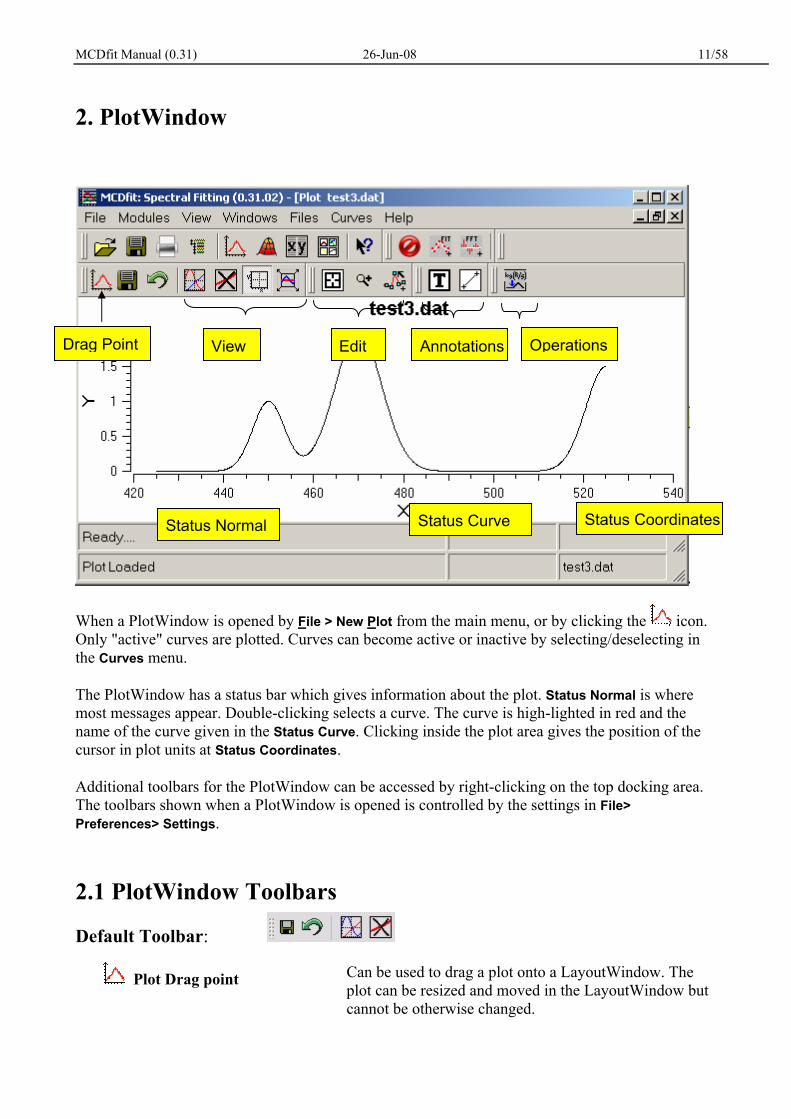
2. PlotWindow

When a PlotWindow is opened by File > New Plot from the main menu, or by clicking the icon. Only "active" curves are plotted. Curves can become active or inactive by selecting/deselecting in the Curves menu.

The PlotWindow has a status bar which gives information about the plot. Status Normal is where most messages appear. Double-clicking selects a curve. The curve is high-lighted in red and the name of the curve given in the Status Curve. Clicking inside the plot area gives the position of the cursor in plot units at Status Coordinates.

Additional toolbars for the PlotWindow can be accessed by right-clicking on the top docking area. The toolbars shown when a PlotWindow is opened is controlled by the settings in File> Preferences> Settings.

2.1 PlotWindow Toolbars

Default Toolbar:

Plot Drag point Can be used to drag a plot onto a LayoutWindow. The plot can be resized and moved in the LayoutWindow but cannot be otherwise changed.

Status CoordinatesStatus Normal Status Curve

Operations AnnotationsEditView Drag Point


Save Curves: When a PlotWindow is created, a copy of the curves is made from the current active file. Clicking this button will save the curves from the PlotWindow back into that file. (Typically after the curves have either their data or their format changed.)

Reload: This re-reads the curves from the PlotWindow file (including their attributes) into the PlotWindow. This can be used to "undo" changes.

Plot Preferences: opens a dialog where the various plotting preferences such as range, auto-scaling, grids, tick intervals, mirror axes, plot styles, etc can be set.

This is where the plot title and axis labels can be changed.

Curve Preferences:

Access by View > Curve Options or clicking on the legend if visible.

Shows the various curve options of the current active curve. These can be changed except for: Name and number of points.

The Line type (none, lines, sticks, steps, dots, spline), style (none, solid, dashed, dotted, dot-dash, dot-dot-dash), width and colour.

The Symbol type (none, circle, square, diamond, up triangle, down triangle, left triangle, right triangle, plus, cross), size, line width, line colour and fill colour.

Change active curves by left-clicking


on them. The active curve is displayed in the middle of the status bar.

Delete Curve: Deletes the current selected curve. The curve can be selected by double clicking on it. (You can also do this from the Curve Menu.)

Axes (toggle): Toggles the axes and plot labels on/off.

AutoScale AutoScales the plot to contain all values.

Filter Toolbar:

A PlotWindow has a default event filter which controls how the mouse and keyboard interacts with the plot. These three toggle buttons install different filters for different mouse/keyboard interaction. See section II.1 for the detailed behaviour. Toggling the button off reverts to the default Plot Filter.

Zoom: When on, an area can be zoomed by click-dragging a square using the left mouse button. When doing successive zooms, clicking the middle mouse button will step back through the previous zoom steps one by one, while the right mouse button will un-zoom straight back to the original size. Toggling the zoom button off will freeze the window in the current zoom state.

Target:

(safe way to examine data)

Left-clicking on a curve will select the nearest point. The coordinates of this point are displayed on the RHS statusbar. The arrow keys ←/→ shift the selected point to the previous/next point. Holding shift down increases each step to 10% of the full scale rather than to next point. The arrow keys ↓/↑ moves the active point to the corresponding point in the previous/next curve. The arrow keys wrap around.

Edit:

(warning changes data)

When on, a point or whole curve can be selected by left or middle double-clicking respectively.

If a point is selected; Left-click dragging will move the point. Right-click will open the popup menu to: Add a point between the current and next point. Delete: delete the current point. Revert: to the last saved curve.

If a curve is selected; Right-click will open the popup menu: Move horizontally: drag whole curve horizontally. Move vertically: drag whole curve vertically. Scale horizontally: stretches whole curve horizontally. Scale vertically: stretches whole curve vertically. Scale: stretches whole curve by corner dragging. Delete: the curve. Revert: to the last saved curve.


Selecting the green or red cursor button, places a vertical cursor at the next position you click in the PlotWindow. Select the cursor by double clicking, these can be dragged and their position (and difference) given in the Coordinates status bar.

When selected the Edit button expands to show cursor buttons

Any change made to the curve data are local changes on the PlotWindow. Press to save that data back to the file if you want to keep the changes.

Functions Toolbar:

The Functions toolbar has the following quick Icons:

Convert to Absorption

Convert to Wavenumber


Smooth

Uses a running average or Savitzky-Golay smoothing.


3. Plot3DWindow When a Plot3DWindow is opened a default example function is loaded.

The icon in the top left corner is the drag point. Use the button will open a mesh file with the extension *.mes.

The Calc button will calculate a surface on the indicated grid using the chosen function .

The button will change the grid. Note that the grid is not used in a parametric function. In this case the variable limits are built into the function.

Clicking the Std button will reset the window to a standard view, while the buttons XY, YZ, XZ project the object onto those planes. These are useful for example when making contour plots.


3.1 Mouse Manipulations Left-click-drags of the mouse can be used to move the Plot3D object.

Move the mouse Up/Down (U/D), Left/Right (L/R) together with combinations of holding down Shift, Alt or Ctrl keyboard buttons.

Rotate Scale X U / D [ALT] L / R Y [SH] L / R [ALT] U / D Z L / R [ALT-SH] U / D Shift horizontal [CNTL] L / R Shift Vertical [CNTL] U / D Zoom [CNTL-ALT] U / D

3.2 View Settings and Options Several Plot3DWindow options become available from the View menu when a Plot3DWindow is open.

When a plot3DWindow is active there are many additional options become visible in the View main menu.

example: View > Axes > box


example: View > Grids > back

example: View > Type > hidden line

example: View > Floor > contour

( adjust Floor offset, plot3D Options > color contours)

example: Floor > elevation

(View > Type > polygon, plot3D Options > color linewidth = 4)


3.3 Defining Functions A user defined function that has been previously defined with 2 variables can be plotted by selecting it from the dropdown menu.

These functions can either be single-valued cartesian, or parametric (see section II 6). For the

single-valued cartesian functions, the x and y – values are equally spaced values over the range (XMin, XMax) (YMin,YMax). With parametric functions the range of the parameters are built into the definition.

Example of a user defined single-valued cartesian function:

A E⊗e Jahn-Teller potential energy surface:

f(x,y) = ½ hw(x2+y2) - [(A1x+A2(x2-y2))*(A1x+A2(x2-y2)) +(A1y-2A2xy)*(A1y-2A2xy) ] ½

View > Style > no data

XY projection

Example of a user defined parametric function:

A dz2 orbital:

x(u,v) = (3*cos(u)*cos(u)-1)*sin(u)*cos(v) y(u,v) = (3*cos(u)*cos(u)-1)*sin(u)*sin(v) z(u,v) = (3*cos(u)*cos(u)-1)*cos(u)


4. TableWindow

This displays the data in the active file in two tables, one with the curve data and the other with curve formatting properties. All curves are displayed, not just the ones marked active.

The data can also be examined and changed using a table. The changes are made immediately to the file. If an open plot is refreshed, it will reflect these changes.

The , and buttons allow table views of the data only, formatting only or views of both data and formatting.

The curve properties of the n curves are displayed in n columns of the property table, each column header has the name of the curve.

Data Table: The data table contains two columns per curve of x- and y-values. The column headers are numbered i[x] and i[y] for curve i. Double-click on the column headers of the data to change the precision and format of the data. Double-click on the column headers of the format table to change the curve names.

Changes to the values can be made directly by editing points. If a PlotWindow and a TableWindow of the same data are both open, then changes in the table are directly reflected in changes of the PlotWindow.


4.1 Generating data from a formula.

Double clicking on or buttons of a Table will open dialogs that give an easy way to create plots of functions.

The "variable" type is an appropriate way to define x-values.

Equally spaced points will be made between the Min and Max values.

The destination is used to determine whether a curve is overwritten or a new curve created.

The "function" type is appropriate to define y-values.

A function can be:

1) chosen from the drop-down box 2) loaded from a previously defined function 3) typed into the f(x)= box directly.

The x- (y-, z-) values are taken from the indicated curves.

A function must be defined in terms of lower case x. The validate button will test the function for the particular x- (y-, z-) values indicated.


5. LayoutWindow

A layout is a canvas on which Plot, Plot3D and Table Windows can be placed for printing.

Each of the Plot, Plot3D and Table Windows has an icon on the upper left of their toolbars which acts as a drag point, eangling them to be dropped onto an open LayoutWindow.

Once on the layout, the objects can be arranged and resized on the layout, they cannot be edited or changed in the way they can when they are in their windows. For example, you can no longer rotate a Plot3D object with your mouse. Selecting an object makes a frame with handles appear, that can be dragged to resize the object. Right click on a selected object allows you to arrange objects that are overlapping, as shown below:

Opens a popup menu with template patterns that can be used to arrange objects.

Zoom in

Zoom out

Selects all objects

Deletes selected objects

Deletes all objects

Insert a Text object at the next place you click on the layout.


5.1 Text Editing

Text objects, which can be added to the layout with the button are exceptions, in that they have extensive editing / formatting capabilities. A selected test object can be edited (right-click > edit text), directly by typing in the text box. A right-click on text being edited allows a formatting window to be open.

The toolbuttons at the top allow the seelcted text to be quickly formatted, ie sub/super-script, change font to symbol, etc.

By default, the text will resize when the textbox is resized on the canvas ("size to fit"). This can be turned off by selecting Fixed.

The colours of the background and text can be changed. Note that button at the right will make the background transparent.


6. MCDexplorer

The MCDexplorer is a tree structure that allows you to examine, organize and link the experimental data from files, the calculated data in models and the parameters in both models and fits.

6.1 Dragging curves between files To move/copy a curve from one file to another, right-click on the curve name and drag the curve to the file name that you want to move it to. A popup menu with the options to move / copy will appear.

6.2 Linking parameters

fileItem curveItem

13 parameterItems

modelItem

4 transitionItems

fitItem

6 parameterItems


The parameters of a fit are colour coded. The parameter type can be fixed (red), varied (green), linked to another parameter (yellow); and another parameter linked to it (purple). Double-click on a parameter to get its name, value and limits.

To link one parameter to another, right-click-drag one parameter onto the other. The dragged parameter will now have the value of the parameter that it has been linked to. Many parameters can be linked to a single parameter, but the linking cannot be "chained". This means that a parameter which has a link to it, cannot be linked to another parameter.

Links can be made by dragging and dropping, or manually by clicking on the "Link" button. The "Unlink" button will remove all links to/from the next parameter you click on.

6.3 Example of using Linked parameters The point of linking parameters is to reduce the number of independent parameters in a fitting process. Some examples where this can be done:

1) Fit a spectrum to a series of peaks that all have the same width. This is appropriate, for example, if you are fitting a Franck-Condon progression.

2) Globally fitting a series of spectra that have been measured on the same sample with different techniques.

a) Electronic Spectroscopy: Absorption, magnetic circular dichroism, and/or circular dichroism

b) Vibrational Spectroscopy: IR and Raman specta

c) Fluorescence Spectroscopy: Fluorescence spectra as a function of excitation.

d) Equilibria of different species

In each case the spectra consist of the same transitions and so will have the same transition energies, but can have different intensities and bandwidths.


7. Module Curve Fit:

Different modules can be selected from the Modules main menu item and also from the MainWindow Modules toolbar.

Selecting the Modules>StartFitting menu item, or clicking on the Fit button, , starts a fit. If a single curve is set "active" in the active file. (These are the curves ticked in the MainWindow>Curves menu), then a single fitWindow (as shown below) is created. If there are multiple curves active in the active file, then a new fitWindow is open for each curve. ie Each curve to be fitted is opened in a separate window.

The ModulesToolbar on the MainWindow expands to the right side of the fit button:

Each fitWindow also has a ModulesToolbar:

Note that there are settings and parameter dialog buttons at a global level as well as for each fitWindow created.


7.1 MainWindow Fit Toolbar

The Fit toolbar on the main window contains buttons that set global options of the fit.

Global Fit Settings This will reopen the dialog for the Global Preferences for the fit.

Global Fit Parameters This will reopen the dialog for the global setting of parameters. The parameters are set locally for each fitWindow (see below) but this dialog allows all parameters to be view together.

Monitor Controls whether the fit updates the plots; turn off to speed up fit.

One iteration Do a single iteration

Start Fit This starts the fit using the current preferences and parameters.

Revert Fit Reverts all parameters to their previous values at the last save.

Save Peaks Opens a dialog where you can saves the fit in a new file with the same name plus an added extension ".fit", and/or save parameters to a "*.par" file.

You can optionally save the fit to a file in Igor format. This will be opened and plotted when dropped into Igor.


7.2 Global Fit Settings Algorithm: A single fitting algorithm is used in a multiple curve fit.

Details: Opens the dialog below for changeable algorithm parameters.

Maximum Iterations: The maximum number of iterations before stopping.

Max. functions calls: The maximum number of function calls.

It. Update: The number of iterations between updates of the plotted curves. ( must be selected)

Points to Sample: The experimental data will be downsized to this number of equally spaced points. (If 0, all points used)

χ2 cutoff: The finishing criteria for the fit. If χ2 changes by less than this number between iterations, the fit will stop. Other stopping criteria are if maximum iterations or maximum function calls is exceeded.

stepChi: The stepsize will be changed on each iteration to the step that increase the parabola at the minima by ChiStep*χ2 (Only active for a "Grid Search")

stepDown: The stepsize

(Only active for a "Gradient Search")

lambda: The stepsize

(Only active for the "Marquardt" algorithm)

Models: The installed models are shown when the "Show available models" button is clicked. One or more models can be selected to be included in the fit. The calculated transition energies and intensities of a model can be linked to the peak parameters position and area respectively. The parameters of the model are then fitted to the spectrum.

plot the model?: Plots the model(s) as a stick spectrum.


7.3 Global Fit Parameters:

Clicking on shows the parameters and the results of a fit. To change the parameters, the curve must be selected in the drop-down menu and the "change parameters" button clicked. This opens a Curve Fit Parameters dialog (see below).

Links

This tab contains the parameters for each fitted curve as a column in the table. The parameters are colour coded according to whether they are fixed (red), varied (green), linked (yellow) to another parameter (purple).

Results

This tab summarizes all parameter results after a fit, both value and an estimate of the error are given.

Correlations

Correlations Tab: A correlation matrix is given as an NxN matrix where N is the total number of


parameters that are varied. This only calculated for the Marquardt and Chi-sq expansion fitting algorithms, not the Grid Search and Gradient Search.

7.4 FitWindow Toolbar

For each FitWindow, a local Fit toolbar has the following buttons:

Fit Settings This will open the dialog for setting the preferences for fitting this curve.

Fit Parameters Opens a dialog for setting the parameters.

Find Peaks Automatic peak-finding routine. Uses settings in the Fit Settings dialog.

Edit Peaks When selected the FitWindow goes into a PeakEdit mode, where a "peak

event filter" is installed, and the toolbar expands to . In this mode, peaks can be selected by double-clicking. A selected peak has three peak handles, one at the peak position and two either side at the full-width at half-height (FWHH) positions. The peak position, height and halfwidth can be changed by dragging these handles. Right-clicking when a peak is selected allows you to set the parameters for this

particular peak. Alternatively, the button , will allow the parameters of any peak or baseline to be changed.

Edit Function When selected the FitWindow goes into a FunctionEdit mode, and the

toolbar expands to . In this, functions can be selected by double-clicking. A selected function has function handles, the position of which depends on the function.

You can define your own functions with your own design of mouse interaction (see section II. 6.2).


7.5 Curve Fit Settings

Data: The full and sampled points are given here, but cannot be changed. Use the global fitting preferences to change the sampled points.

Show residuals: A residuals curve (exp-calc) curve is plotted in green.

Show zero line: A zero line is plotted as a dotted line.

Allow negative peaks: Usually peaks are restricted to being positive, but sometimes (CD, MCD) negative peaks are desired.

Restrict fitting range: Fits can be restricted to a certain range of x-values.

Peak Pick: The automatic peak-picking routine can be controlled using these parameters. To be picked, the peaks must be over the threshold value (as % of maximum y-value), with a FWHH that lies between minimum and maximum values. The highest peaks up to Max.Peaks are returned. A smoothing factor is used to minimize the effects of noise in the spectra.

PeakType: The shape of the peak to be fitted. (choices are: Gaussian, Poisson, Voigt, Lorentzian)

Show Peaks: Curves for the individual peaks are shown.

Labels On: Peaks labels. Right clicking on labels allows editing.

Baseline: Choices are: None, Offset, Linear, Polynomial, Spline.

Tie Points: The number of points used to represent the Polynomial or Spline. An nth degree polynomial requires n+1 points.


7.6 Curve Fit Parameters

The type of background can be changed with the drop-down menu.

Peaks Tab: The peak parameters are given, with a horizontal slider to change between peaks. The peaks are energy ordered from left to right. Parameters can be fixed or variable. There must be at least one variable parameter for a fit to be made.

Limits Tab: Limits of the particular peak selected in the Peaks Tab.

The Spline and Polynomial Tabs only become enabled when the appropriate baseline is chosen. The Offset and Linear baselines are considered to be polynomials of degree 0 and 1. Both splines and polynomial backgrounds are parameterized by tie points which are draggable handles in peakEdit mode.

During the fit the y-values of the tie points can be varied, the x-values remain where they have been placed. A polynomial of degree n requires n+1 points to be uniquely specified.


7.7 Peak Parameters (right-click on active peak in PeakEdit mode .)

This dialog is obtained by right-clicking on a selected peak. It allows the parameters of that particular peak to be changed.


8. Module: Fourier Analysis

Invoke the FFT (Fast Fourier Transform) module with the Modules > Start FFT menu or the

button on the modules toolbar. The toolbar menu expands to . The first new button opens a dialog for general FFT settings.

Name: Curve being processed

Original points: in the original curve

FFT points: zero padded to be a power of 2.

Nyquist limit: the

f/t sampling: the

auto update windows?: When windows are dragged the curves are automatically recalculated.

auto update forward FFT?: Changes in the frequency domain are automatically updated in the time domain window.

auto update back FFT?: Changes in the time domain are automatically updated back into the frequency domain window.

AutoScale


Each of the frequency and time domain windows has a

settings dialog button . This opens a dialog which allows the window type and parameters to be set.

The FFT windows are visible if is toggled on. The window parameters can be changed by double-clicking and dragging the handles, and the window type by right-clicking on a window.

Show Log in T domain?: Set the y scale to logarithmic, as the FT usually has positive and negative values, you will probable want to set the Show T magnitude?, which will give the absolute values of the FT.

The FT in the frequency domain is given with the same x-axis as in the time domain, unless the Show actual T-axis? is selected.

Each window has the toolbar above, which allows the three curves displayed to be toggled on/off.

The button causes and explicit forward Fourier transform and updates the contents of the time domain window. Likewise, the button in the time domain window causes an explicit back

Fourier transform and updates the contents in the frequency domain window. The button brings

up the "quick help" manual, usually to find out which colours correspond to which curves. The button refreshes the curves.

Frequency Window Time Window

original curve (black)

FFT → FT (black)

doesn't change

↓ zero pad, × by window

windowed curve

(blue)

FFT → FT of windowed curve

(blue)

changes as window in frequency domain changes

↓ × by window


back FFT (green) ← backFFT filtered FT (green) changes as window in time

domain changes

In the above example, note that as you move the window in the time domain to cut off the high frequency components, that the noise in the spectrum is reduced.


9. Models: PES Calculates transitions between two one-dimensional potential energy surfaces (PES). Assumes that the transitions are allowed and the intensity is given by the overlap of the vibrational wavefunctions. This is appropriate, for example, for calculating the Franck-Condon pattern for displaced potential energy surfaces, where the displacement is along a totally symmetric vibrational coordinate. It is not appropriate fro transitions that are vibronically allowed, for example “ungerade” modes in centrosymmetric molecules. The potential surfaces are described by a polynomial up to 4th order and the energies and wavefunctions are calculated by evaluating the vibrational Hamiltonian using harmonic basis functions and diagonalising the resulting matrix. A 4th order polynomial is also capable of describing a double minima PES.


The ground and excited state potential energy surfaces are described as polynomial expansions up to 4th order

where n = g, e for ground and excited states respectively. The vibrational Hamiltonian to be solved is


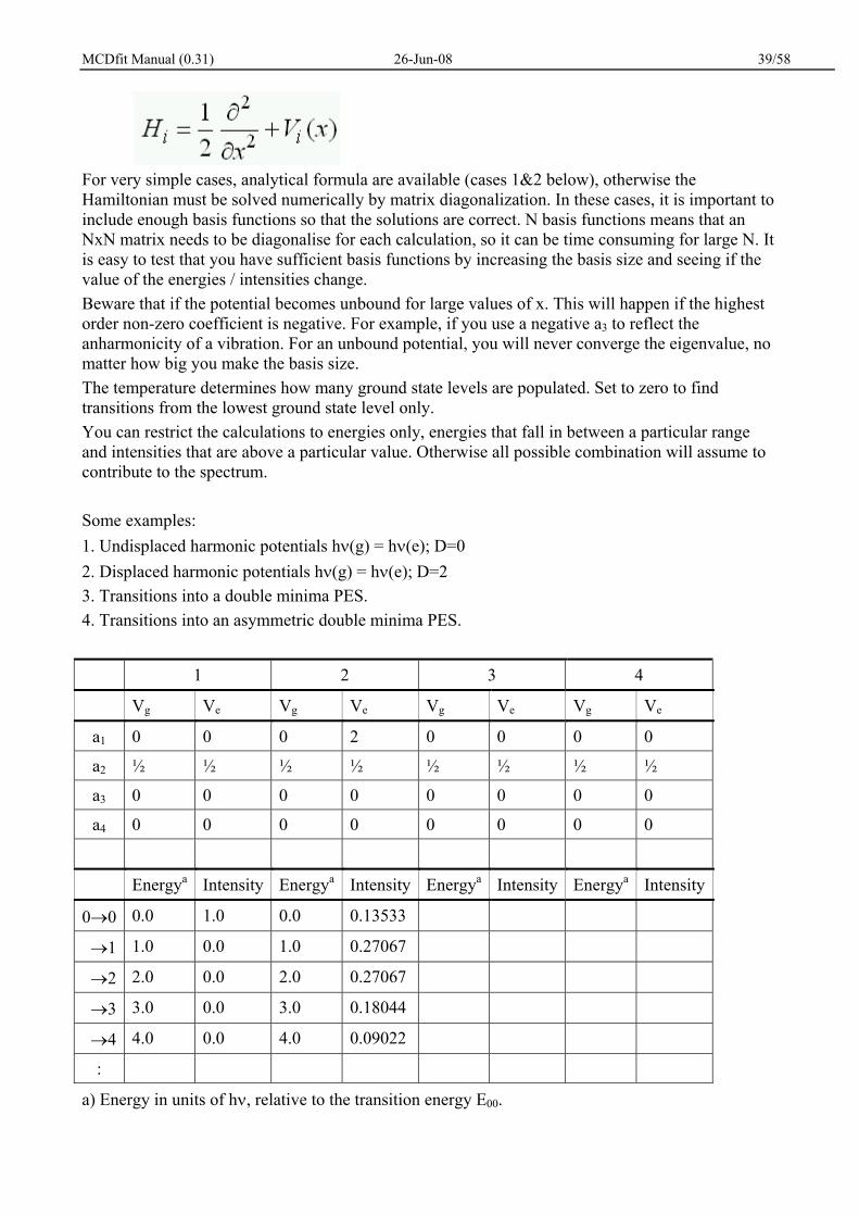
For very simple cases, analytical formula are available (cases 1&2 below), otherwise the Hamiltonian must be solved numerically by matrix diagonalization. In these cases, it is important to include enough basis functions so that the solutions are correct. N basis functions means that an NxN matrix needs to be diagonalise for each calculation, so it can be time consuming for large N. It is easy to test that you have sufficient basis functions by increasing the basis size and seeing if the value of the energies / intensities change. Beware that if the potential becomes unbound for large values of x. This will happen if the highest order non-zero coefficient is negative. For example, if you use a negative a3 to reflect the anharmonicity of a vibration. For an unbound potential, you will never converge the eigenvalue, no matter how big you make the basis size. The temperature determines how many ground state levels are populated. Set to zero to find transitions from the lowest ground state level only. You can restrict the calculations to energies only, energies that fall in between a particular range and intensities that are above a particular value. Otherwise all possible combination will assume to contribute to the spectrum. Some examples: 1. Undisplaced harmonic potentials hν(g) = hν(e); D=0 2. Displaced harmonic potentials hν(g) = hν(e); D=2 3. Transitions into a double minima PES. 4. Transitions into an asymmetric double minima PES.

1 2 3 4

Vg Ve Vg Ve Vg Ve Vg Ve

a1 0 0 0 2 0 0 0 0

a2 ½ ½ ½ ½ ½ ½ ½ ½

a3 0 0 0 0 0 0 0 0

a4 0 0 0 0 0 0 0 0

Energya Intensity Energya Intensity Energya Intensity Energya Intensity

0→0 0.0 1.0 0.0 0.13533

→1 1.0 0.0 1.0 0.27067

→2 2.0 0.0 2.0 0.27067

→3 3.0 0.0 3.0 0.18044

→4 4.0 0.0 4.0 0.09022

:

a) Energy in units of hν, relative to the transition energy E00.


10. Functions

10.1 Convert to Absorption The selected curve (or the only curve if there is only one in the active PlotWindow) is treated as a transmission curve. Other curves in the file are listed in a drop down list as possible baseline curves. The absorption is calculated as

where I0 is the baseline curve and Is the transmission curve of the light going through a sample. The baseline curve I0 must cover the range of the transmission curve Is and must be in the same units (ie cm-1, nm, etc..). The spacing need not be the same, appropriate values for I0 will be interpolated.

10.2 Data Smoothing The curve in the file will be in the drop-down list with the selected curve the current item. Smoothing algorithms include a simple running average and Savitzky-Golay smoothing.

Running average: The number of points averaged is 2N+1, which must be an odd number. If points=1, this is the same as no averaging.

Savitzky-Golay: Here the number of points to the left and to the right are set equal NL = NR = N. The coefficients cj are chosen to preserve a particular moment M of the fitted region. If M=0, then the zeroth moment (or area under) the fitted region is preserved. In this case the coefficients reduce to 1/(2N+1), and the Savitzky-Golay smoothing is the same as a running average. Higher moments preserve sharp features, but do less smoothing on broad features. (see [3] ch.14.8)

10.3 MCD Analysis Using this option, the shape function used to fit the spectra will be of the form

where f and f' is the shape function and its first derivative; C is a constant, µB is the Bohr magneton, and B the magnetic field strength (Tesla). A1, B0, C0 are parameters used to describe the MCD spectrum. See [2].


Part II Reference

1. Mouse / Key actions Mode Double-Click Left-click Middle Right-click

Left: On curve: Selects (highlights) the current curve. Only curves, not peaks are considered. On text/tag/line object: Select current object, once selected it came be dragged and edited (with right click)

On curve: show curve name. On text/line: Allows the item to be dragged. If "add text/line" previously selected from the right-click popup, then the items will be added at the cursor position.

- If a curve is selected, a curve format dialog opens. If a text/line is selected, a popup menu opens with options for add/cut/copy/properties/ etc.

Plot

All button clicks show the coordinates at the cursor at RHS status. Current curve name is shown in the middle status bar.

- Start a zoom selection. Selection will finish when button released.

Go back one in zoom stack.

Go back to beginning of zoom stack and autoscale.

Zoom

Left: Selects a point which can then be dragged. Point highlighted. (right-click for popup options) Middle: Selects a curve which can then be dragged. Curve highlighted. (right-click for popup options)

Allows a selected point to be dragged.

- Popup context menu If point selected options are: delete add (after current) revert to saved curve If curve selected options are: move vertically move horizontally scale vertically scale horizontally scale arbitrary delete revert to saved curve

Edit

- Selects a point Position shown in status bar.

- - Target

← → move to next point. (+shift key moves by ±10% of full range) ↑↓ move to next curve. (wraps around) The selected point (not cursor) shown in RHS status bar.


Mode Double-Click Left-click Right-click

PeakEdit

When the tick / cross is toggled, peaks are added / deleted at the next cursor click.

Select/deselect peaks or baselines for editing. The peak handles are highlighted. (Only peaks, not curves are considered)

If a peak is selected: Left-click drag at the anchor points of the peak handle. Similarly, the handles of a baseline can also be dragged.

If peak is selected: A dialog opens that allows you to change the parameters of the selected peak. If a baseline is selected: a right-click opens a popup menu where the baseline handle points can be added or deleted.

FunctionEdit

When the tick / cross is toggled, functions are added / deleted at the next cursor click.

Select/deselect functions for editing. The function handles are highlighted when selected..

Selected functions can be dragged by the handles

If a function is selected, this will open a dialog allowing you to change the parameters of the selected function. You can also change the function type to any that have been previously defined.

Note: Plot mode is the normal for mouse actions, unless one of the other toggle buttons is on. Only one of the toggle buttons is allowed to be active at any one time. PeakEdit and FunctionEdit are only allowed when a fit is in progress.


2. Shortcut Keys:

Key Menu Equivalent Action

F1 Help > Quick Help Brief Help: Command line options; Mouse actions; Fitting curve colours.

F2 Help > Users Guide Full User Guide. (This document).

F3

F4

F5

F6 Windows > Close All Windows

Closes all windows.

F7 Files > Close All Files Closes all files.

F8

F9

F10

F11

F12

Crtl+F Operations > Start Fit Starts fit & opens the Fit Toolbar.

Ctrl+O File > Open Opens a new file.

Ctrl+P File > New Plot Opens a new window with a plot, with curves from the current file. Default plot if no file open.

Ctrl+S File > Save Save current file.

Ctrl+T File > New Table Opens a new window with a table, with entries from curves in the current file. Default table if no file open.

Ctrl+Q File > Quit Quit MCDfit.

Shift+F1 Help > Whats This? Enables context help on next item clicked. Turns off after this.


3. Command Line Options

The program can be run by typing MCDfit at the prompt. The command line options for a normal user are as follows:

> MCDfit [-user user] [-u user] start with username user [-help] [-h] display this help and exits [-version] [-v] displays program version and installed modules

4. Settings File & User Login:

There is a file MCDfit.ini that is always read when the program starts up. It is in the home directory which where the MCDfit.exe program is. This contains a list of users. When the program is started with a login name ie >MCDfit -u name, then a file name.ini is read from the home directory. This file contains some previous settings of the user when they last exited the program normally. One can also dispense with the logins by deselecting the User Login checkbox (File>Preferences>User Settings). If this is deselected, the next time the program is run will be with the default settings.


5.0 Fitting algorithms The fitting algorithms are non-linear least-squares fitting routines taken from “Data Reduction and Error Analysis for the Physical Sciences” P.R. Bevington & D.K. Robinson, 3rd Ed. McGraw-Hill, 2003. The routines can be obtained from http://www.mhhe.com/bevington and are C++ translations from Fortran77.

The χ2 function to be minimized is given by:

χ2 = Σ { [yi-y(xi)]2 / σi2 }

where xi and yi are the measured values and σi is the uncertainty in yi, and y(xi) are the calculated values of the fitting function at xi.

Successful fitting of non-linear functions can depend on the choice of method, the choice of starting parameters and the choice of step-size. Unlike linear least-squares, one is required to provide both starting values and step-sizes.

Local Minima: A common problem is the existence of multiple local minima. For an arbitrary function there may be more than one minimum in the χ2 function within a reasonable range of parameter values. A particular choice of starting parameters may drive the solution towards a local rather than the global minimum.

Bounds: Another problem may be that the search may converge towards parameters that are known to be unreasonable; for example a particular problem may be restricted to positive peaks (or positive peak areas). This situation is avoided by specifying lower and upper limits or bounds on each parameter and a “penalty” is added to the χ2 function that depends on the extent that the parameter penetrates the forbidden region.

Step-size: The step-size is different for different parameters and is related to the slope of the χ2 function. Very small step-sizes will be slow to converge, very large steps will overshoot. In these routines the initial step-size proportional to the initial value of the parameters and adjusted through the search.

Convergence: The problem is said to converge when the change in the χ2 function per degree of freedom (χ2 / dof) falls below a certain value. This may result in a search stopping in a very flat valley. In which case one can restart from a different starting position or set a tighter convergence criteria.

The four routines used are described in chapter 8 of the Bevington & Robinson book [1].

1. Grid Search: The χ2 function is minimized with respect to each parameter ai separately. The disadvantage of this method is that if the parameters are strongly correlated, then the convergence may be slow. The calculated uncertainties correspond to the diagonal elements of the error matrix and are therefore inaccurate if correlations are important.

2. Gradient Search: In this method all parameters ai are incremented simultaneously with relative magnitudes adjusted so that travel is along the maximum variation in χ2 in the direction of steepest descent. The efficiency of this type of search decreases as the minimum is approached and the gradient decreases. The Gradient Search is usually much quicker than the Grid Search;


however it may tend to get stuck in long shallow valleys compared to the Grid Search which eventually reaches a right answer.

3. χ2 Expansion: Instead of searching the hyperspace of χ2 as a function of parameters ai, χ2 is approximated by a parabolic expansion. This requires the inversion of a matrix of the dimension of the number of parameters and the 1st and 2nd derivatives χ2 with respect to the parameters.

4. Marquardt Method: One disadvantage of the above procedure is that although it converges rapidly from nearby points, it cannot be relied to converge outside the region where the χ2 hypersurface can be approximated as parabolic. In contrast, the Gradient Search is ideal for approaching the minimum from a distance. The actual path directions for the Gradient and Expansion methods are nearly perpendicular to each other and the optimum direction is somewhere in between. This strategy was used by Marquardt in a Gradient Expansion (or Marquardt) method. The Marquardt method is reasonably insensitive to the starting values of the parameters and provides a full error matrix.

5.0.1 Error estimates of the fitted parameters

The fitted parameters also return uncertainties of their values as standard deviations, σi. How they are calculated, depends on the fitting algorithm used.

For the Grid Search and the Gradient Search methods, an estimation of the uncertainties, σi is set as the values of the parameters ai required to increase the parabolic approximation to the χ2 function by 1 from its minimum value.

For the χ2 Expansion and Marquardt methods, a full error matrix is calculated which given where the errors are the square roots of the diagonal elements and the covariances between parameters ai and aj are the off-diagonal elements εij. These have been divided by σi and σj, so values near ±1 indicate that parameters ai and aj are highly correlated.

Errors on fitting the file Test3.dat

A1 err P1 err ∆1 err A2 err P2 err ∆2 err Grid Search 8.8627 1.1195 450.00 0.6316 8.3259 1.2144 26.2892 1.3657 470.00 0.3906 12.3486 0.7633

Gradient Search 8.8609 1.1194 450.00 0.6322 8.3240 1.2071 26.2873 1.3656 470.00 0.3909 12.3473 0.7567

χ2 Expansion 8.7949 1.4375 449.99 0.6403 8.2629 1.6911 25.984 1.8146 469.97 0.3906 12.1884 1.1157

Marquardt 8.8087 0.0352 449.99 0.0199 8.2818 0.04077 25.9978 0.04289 469.97 0.0122 12.1981 0.0258

Ai, Pi and ∆i are the area, peak and FWHH of peak i.

5.1 VARPRO: Separable nonlinear least squares: the variable projection method.

Background: The variable projection method for solving separable nonlinear least-squares problems [7, 8] is suited to those problems where the model function is a linear combination of nonlinear functions. Taking advantage of this special structure, the method of variable projections eliminates the linear variables obtaining a more complicated function that involves only the nonlinear parameters. This procedure not only reduces the dimension of the parameter space but also results


in a better-conditioned problem. This method is ideally suited to spectroscopic problems which are usually modeled as a linear combination of (non-linear) peak functions.

If there are S sets of N observables of the dependent variable: Y1,1, ... YN,S, where each YI,J observable corresponds to the positions of the IV independent variables Ti,1, Ti,2 ... Ti,IV, the algorithm makes a (weighted) least-squares fit to a function, ηk, which is a linear combination of the non-linear functions Φ.

ηk(α, β; T) = ∑=

L

1jβj,k Φj(α; T) + ΦL+1(α; T)

That is, determine the linear parameters βj,k for j=1,2,...,L, K=1,2,...,S, and the vector of the NL non-linear parameters α by minimizing the Frobenius norm of the matrix of residuals:

Norm2 = ∑=

S

1k∑=

N

1iWi [Yi,k - ηk(α, β; T) ]2

In the version used here, addition there is an implementation that considers sets of observables that depend on the same independent variables and have different values of the linear coefficients, β, but are constrained to have the same nonlinear parameters α [9].

The ΦL+1 is for a constant non-linear function. When S >1 the multiple right hand sides are allowed to have different values of the linear coefficients, β, but are constrained to have the same nonlinear parameters α [8]. The above form for ηk(α, β; T) is called "separable", a non-separable case is when L=0 and just using ΦL+1(α; T). A linear least squares case is that where NL = 0. The algorithm requires the partial derivatives of Φ with respect to α. An advantage of the VARPRO algorithm is that no initial guesses are required for the linear parameters.

5.1.1 Application of VARPRO in MCDfit

The VARPRO method is ideally suited to spectroscopic problems which are usually modeled as a linear combination of (non-linear) peak functions. In addition the sets (S>1) of data are ideal for multiple curve deconvolution, where spectra over the same wavelength range are used. The same peak functions can be assumed for the spectra that have been measured using techniques that depend on different selection rules (ie the spectra have the same transitions). It may be that some of the spectral peaks will be zero in some spectra. In some spectra like the Raman and IR spectra of centrosymmetric molecules, there will be no peaks in common. The peaks corresponding to the transitions are the same in both spectra, but peak appearing in one spectrum will have zero intensity in the other (mutual exclusion rule).

6. User defined functions

6.1 Built in functions There are a number of "hard-wired" shapes to use in spectral fitting:


• Gaussian • Lorentzian • Gaussian derivative • Lorentzian derivative

It is also possible to define your own functions that can be used in the fit. To do this, provide an expression in terms of the variable "x" and parameters values "a0", "a1", "a2", .... The expression for the function is parsed and evaluated using proper precedence by the "muParse"[4] parser. The function expression can use any of the following built in operators/functions:

unary operators - negation binary operators + - * / arithmetic operators ^ raise to a power defined functions abs(x) acos(x) acosh(x) asin(x) asinh(x) atan(x) atanh(x) avg(x1,x2,x3,...) Average value of a list of arguments separated by commas bessel_j0(x) Regular cylindrical Bessel function of zeroth order, J0(x). bessel_j1(x) Regular cylindrical Bessel function of first order, J1(x). bessel_jn(x,n Regular cylindrical Bessel function of nth order, Jn(x) cos(x) cosh(x) exp(x) gamma(x) Computes the Gamma function, subject to x not being a negative integer gammaln(x) Computes the logarithm of the Gamma function, subject to x not a being negative

integer. For x<0, log(|Gamma(x)|) is returned if(e1,e2,e3) if e1 is true, e2 is executed else e3 is executed ln(x) natural log of x log(x) decimal log of x log2(x) base 2 log of x min(x1,x2,x3,...) Minimum of the list of arguments max(x1,x2,x3,...) Maximum of the list of arguments rint(x) Round to nearest integer sign(x) Sign function: -1 if x<0; 1 if x>0 sin(x) sinh(x) sqrt(x) tan(x) tanh(x)

6.2 Definition of function handles


Part of the usefulness of the curve fitting module is the interactive nature of being able to drag the functions using drag-handles. These adjust the parameters of the function to the shape that is being dragged. To enable this for a user defined function, you must provide the following information:

A. The handle positions as a function of the parameters. B. The parameters as a function of the handle positions C. Whether the handles can be dragged (or not) in the vertical/horizontal directions. D. Adjustment of the x-values of the handles to guarantee the function will be single valued. E. How the handle positions are linked. F. The default & limiting values of the parameters for a particular plot.

To illustrate this we will specify the above for one of the built in functions.

y(x) = a1 + a2 exp[-(x-a0)/a3 ] for x ≥ a0 (1) = a1 x < a0

Such a function could be used, for example, to fit an exponential decay of a fluorescence lifetime measurement.

The function is plotted above with the three handles. A choice of handles is not unique, but you need at least n/2 handles to specify n parameters. The definition of the handles in terms of the parameters is a non-trivial exercise. It is well-worth giving it some thought to make the handles intuitive to used.

A. The positions of the handle points shown above can be expressed as a matrix:

h = A a (2)

(a0, a1+a2)

(a0 + a3 ln(2), a1+½ a2)

(a0 - δ, a1)

y(x)

0

1

2

x


=

3

2

1

0

y

x

y

x

y

x

aaaa

01/210ln20010100000100100001

221100

Once you have defined the matrix A above, the rest is straight-forward.

B. When the handles are dragged by the mouse, the parameters are changed according to the positions of the dragged handles:

a = B h (3)

−−−

−=

y

x

y

x

y

x

3

2

1

0

221100

02ln

102ln2

102ln2

1001010

1/301/605/600001/201/2

aaaa

The 4×6 matrix B is the "pseudo-inverse" of the 6×4 matrix A. It should have the properties:

B A = a 4×4 identity matrix A B = a 6×6 symmetric matrix

Use Octave/Mathematica to do the work.

C. The movements of the three handles are restricted such that handle 0 can only be dragged vertically, handle 1 both horizontally and vertically, and handle 3 horizontally only. The 4 degrees of freedom are required to be able to change all 4 parameters of equation (1) above.

0

2

1


With these choices, handle 0 determines the vertical offset a1, 1 determines both the amplitude a2 and the horizontal offset a0, while 2 while determine the time constant a3. This behaviour is built into equation (2). The "draggability" can be expressed as:

=

TTF

210

x

x

x

=

FTT

210

y

y

y (4)

D. Equation (2) will make the x-values of the handles 0 and 1 equal. This is undesirable as we wish to always have single valued functions, so we move 0x to the next lowest value, which will be a0-δx, where δx is the stepsize of the fitting function.

The adjustment vector δ is added to h after it is calculated from (2) and before h is plotted.

Similarly, after a handle has been dragged, the vector δ is subtracted from h before the parameters are calculated from (3). In this example adjustment vector δ is given by

−

=

00000δx

δ (5)

Here the δx is the smallest distance between two x-values, the x-value spacing. In practice, these adjustments are very rarely necessary in defining handles.

E. When a handle is dragged, the behaviour can be more complicated then just a single point of the handle moving. For example, when 0 is dragged vertically to change a1, ideally we would want the handles 1 and 2 to also shift vertically by the same amount. Otherwise if only 0 moved, then both a2 and a3 would change, as well as a1, when 0 is dragged.

Other desirable "linked" behaviour includes:

When 1x is dragged horizontally: 0x and 2x should also move.

When 1y is dragged vertically, 2y should also move so that it remains halfway between 0y and 1y.

The following matrices link the handle movements to give the above behaviour. i.e. a mouse drag of 2 so that ∆2x changes, also causes ∆1x to change. The columns marked • indicate handle directions that are not draggable (in this case ∆0x and ∆2y).


∆∆∆

•••

=

∆∆∆

x

x

x

x

x

x

210

110101

210

'

'

'

∆∆∆

•••

=

∆

∆

∆

y

y

y

y

y

y

210

2/12/11101

2

1

0

'

'

'

(6)

F. The default values of the parameters, and therefore size, of a defined function depends on the particular scale of a plot being made. We defined the default values and the minimum and maximum values in terms of the range of x- and y-values of the plot.

default:

−−

=

YmaxYminXmaxXmin

005/15/12/12/100

0000002/12/1

aaaa

3

2

1

0

(7)

low:

−−

=

YmaxYminXmaxXmin

00)2ln(10/1)2ln(10/120/120/10001000008.0

aaaa

3

2

1

0

(8)

high:

−−

=

YmaxYminXmaxXmin

00)2ln(/1)2ln(/12/12/100

1000002.10

aaaa

3

2

1

0

(9)

The above choices are arbitrary, but will result in reasonable behaviour. These values are commonly used to set values when the function has changed.

6.3 Editing a function The userFunction Dialog (modules > Define Function) allows you to construct a user defined function, including the definition of the handles expressed by the matrices in (2)-(6). It will also test the definition to make sure that it is sensible.

Once you have defined a useful working handle, save it to a file *.fun. These files are then available to load at later sessions.


7. File Formats

7.1 ASCII data format (*.dat)

The basic input file is an ASCII text file (can be read by any simple text editor) with the extension '.dat'. If a line starts with a '#' (in column 1) and the next word is not a 'keyword' then the line is treated as a comment. There may be an arbitrary number of comments in the file. If a line does not have a '#' in column 1 then it is treated as data.

If the '#' is followed by one of the following keywords, then it sets some properties of the curves.

Currently defined keywords: # curve_name Each contiguous name on this line is the name of a curve.

There can be many curve_names on this line. The names may be separated by whitespace (space, comma, tab, ) default: "# curve_name curve_1, curve_2, ...

The data may be either given as single x, y pairs, one pair per line, or multiple curves with common x-values in the form: x1, y11, y21, y31 ... ym1 (commas can also be spaces or tabs) x2, y12, y22, y32 ... ym2 x3, y13, y23, y33 : x4, y14, y24, y34 : : : : : : xn, y1n, y2n, y3n ... ymn In this case there are m curves, each with the same number of n points and with the same x-values. The first m curve_names are assigned to these curves, or default values used if less than m curve_names provided. A '#' can be used to separate different blocks of data. ie You can have a curve as a block of x, y pairs; followed by a block of 3 curves with common x-values, following by a block of 2 curves with common x-values, each block being separated by a line with a "#". Alternatively these 6 curves can be given as 6 separate blocks of x, y pairs.

7.2 Other file formats (*.par, *.itx) A *.par file contains parameters from a previous fit. Since it is written by MCDfit program, you don't need to know the exact format. Make sure you have a fit open before you reload the parameters of a previous fit from a *.par file. A *.itx file, is an Igor text file. Only the data is read, all formatting is lost.


7.3 Grid data format (*.mes) As specified in qwtplot3d [6] jk:11051895-17021986 // magic string MESH // MESH file (other keywords in future versions) 327 466 // x,y grid 557726 567506 // domain boundaries (x values) 5.10821e+006 5.12216e+006 // domain boundaries (y values) 682 682 682 682 912 924 928 928 932 ... ... element[327*466-1] // the single z values

7.4 Function definition (*.fun) The input specification of the formula/function files enables different types of formulae (in cartesian, cylindrical, and spherical coordinates). The formula must be a valid C expression. A formula parser [4] recognizes operator precedence and constants that can also be defined in the function. It generates byte code, which makes it extremely fast. A function is a formula that also has information about handles that allows mouse interaction. In general a line that is read in as a string will also read any trailing comments. Therefore don't leave comments in the lines marked with red. data read as a known number of numerical values are OK.

# comment MCDfit version:0.31 // formulaName // formulaLabel // formulaComment // nV, nP, nC, nH, nCond // nV, nP, nC, nH, nCond constantsName(i), (i=1, nC) // all constant names on single line constantsValue(i), (i=1, nC) // all constant values on single line constantsComment(i) // each constant comment on new line (line repeated nC times) Condition(i) // each condition on new line (line repeated nCond times) ConditionFormula(i) // each conditionFormula on new line (line repeated nCond times) formulaEq // if nP!=0, this line repeated 3 times -------------------------------- Above here is a formula; below defines function positive[0] ... positive[i] // i form 0 to nC-1 default[0][0], .. default[0][4] // default[i][0], .. default[i][4] // i from 0 to nC-1 low[0][0], .. low[0][4] // low[i][0], .. low[i][4] // i from 0 to nC-1 high[0][0], .. high[0][4] // high[i][0], .. high[i][4] // i from 0 to nC-1 -------------------------------- // below here only for nH>0. aToH[0][0], aToH[0][j] // j from 0 to nC-1 : aToH[i][0], aToH[i][j] // i from 0 to 2*nH-1 draggableX[i], draggableY[i] ... // for i from 0 to nH-1 dX[0] .. dX[i] // i from 0 to nH-1 hToA[0][0], .........hToA[0][j] // j from 0 to 2*nH-1 : hToA[i][0], .........hToA[i][j] // i from 0 to nC-1 linkX[0][0], .. linkX[0][j] // j from 0 to nH-1 : linkX[i][0], .. linkX[i][j] // i from 0 to nH-1 linkY[0][0], .. linkY[0][j] // j from 0 to nH-1 : linkY[i][0], .. linkY[i][j] // i from 0 to nH-1


7.5 User Defined Constants (*.con) The file data\constants\userConstants containing global constants is read in at startup. The user can define constants by editing this file. Each constant is defined in 2 lines: pi 3.141592654 // name (must be contiguous) and the value. Trigonometric pi // comment (may be blank). k 0.695 // name Boltzmann’s constant in units of cm-1 / K // comment Constants can also be edited in the User Globals Dialog, where the constants in the table are those currently in memory. Constants can be added (Add) and delete individually (select row & Delete) or the whole table deleted (Clear). Additional constants may be loaded from a file (Load) or current constants save to a file (Save).


8. GPL Licences Documentation copyright: ©2007 Mark Riley [email protected]

Permission is granted to copy, distribute and/or modify this document under the terms of the GNU Free Documentation Licence, version 1.1 or any later version published by the Free Software Foundation, with no Invariant Sections, with no Front-Cover Texts, and with no Back-Cover Texts.

Program copyright: ©2004-8 Mark Riley [email protected]

This program is free software; you can redistribute it and/or modify it under the terms of the GNU General Public License as published by the Free Software Foundation; either version 2 of the License, or (at your option) any later version.

9. References: [1] PR Bevington & DK Robinson, "Data Reduction and Error Analysis", 3rd Ed., McGraw-Hill,

2003. [2] SB Piepho & PN Schatz, "Group Theory and Spectroscopy", Wiley, 1983, ch. 4. [3] WH Press, SA Teukolsky, WT Vetterling, BP Flannery, "Numerical Recipes in C++", 2nd Ed.,

Cambridge Uni.Press, 2002. [4] muParser, ver 0.2.6, sourceforge.muparser.net

[5] Qwt, 5.0.2, sourceforge.qwt.net

[6] Qwtplot3d, 0.2.7, sourceforge.qwtplot3d.net

[7] G. Golub & V. Pereyra, Inverse Problems 2003 , 19 R1-R26. "Separable nonlinear least squares: the variable projection method and its applications"

[8] B. W. Rust, Computing in Science & Engineering, M arch/April 2003, pp. 74-9. "Fitting Nature's basic functions Part IV: The variable projection algorithm."

[9] G. Golub & R. Leveque, Proc. 1979 Army Num. Anal. & Computers Conf., ARO REPORT 79-3, pp. 1-12. "Extensions and uses of the variable projection algorithm for solving non-linear least squares problems."


Part III Debugging In a debug version of the program can be built by defining the preprocessor flag: _DEBUG. The following toolbar is added to the main window toolbar:

Debug toolbar: (hidden in release versions)

expands to and adds a debug toolbar to every open plot/fit window The button lists all Widgets in a tree structure. File > Preferences > Debug

This controls whether debugging information is sent to the console. (This menu item is disabled on release versions of the program.) Debugging a Class means that lots of output will be printed to the console. If -ctor and/or -dtor is used without and -class options, then all constructor and destructor calls are traced. If -ctor and/or -dtor is used with any number of -class options, then just these constructor and destructor calls are traced. The information returned is in the form: > ctor classname (n) address

(n) is the number of classname objects that exist after the constructor or destructor has been called.

multiple curve deconvolution and fit - sourceforgemcdfit.sourceforge.net/manual_0_31_03.pdf · bw...

Documents