multiple audio sources detection and localization guillaume lathoud, idiap supervised by dr iain...
TRANSCRIPT

Multiple Audio Sources Detection and Localization
Guillaume Lathoud, IDIAP
Supervised by Dr Iain McCowan, IDIAP
Outline
• Context and problem.
• Approach.– Discretize: ( sector, time frame, frequency bin ).– Example.
• Experiments.– Multiple loudspeakers.– Multiple humans.
• Conclusion.

Context
• Automatic analysis of recordings:– Meeting annotation.– Speaker tracking for speech acquisition.– Surveillance applications.

Context
• Automatic analysis of recordings:– Meeting annotation.– Speaker tracking for speech acquisition.– Surveillance applications.
• Questions to answer:– Who? What? Where? When?
• Location can be used for very precise segmentation.

Microphone Array


Why Multiple Sources?
• Spontaneous multi-party speech: – Short.– Sporadic.– Overlaps.

Why Multiple Sources?
• Spontaneous multi-party speech: – Short.– Sporadic.– Overlaps.
• Problem: frame-level multisoure localization and detection. One frame = 16 ms.

Why Multiple Sources?
• Spontaneous multi-party speech: – Short.– Sporadic.– Overlaps.
• Problem: frame-level multisoure localization and detection. One frame = 16 ms.
• Many localization methods exist…But:– Speech is wideband.– Detection issue: how many?

Outline
• Context and problem.
• Approach.– Discretize: ( sector, time frame, frequency bin ).– Example.
• Experiments.– Multiple loudspeakers.– Multiple humans.
• Conclusion.

Sector-based Approach
Question: is there at least one active source in a given sector?

Sector-based Approach
Question: is there at least one active source in a given sector?
Answer it for each frequency bin separately
Frame-level Analysis
f
s
Sector
of space
Frequency bin
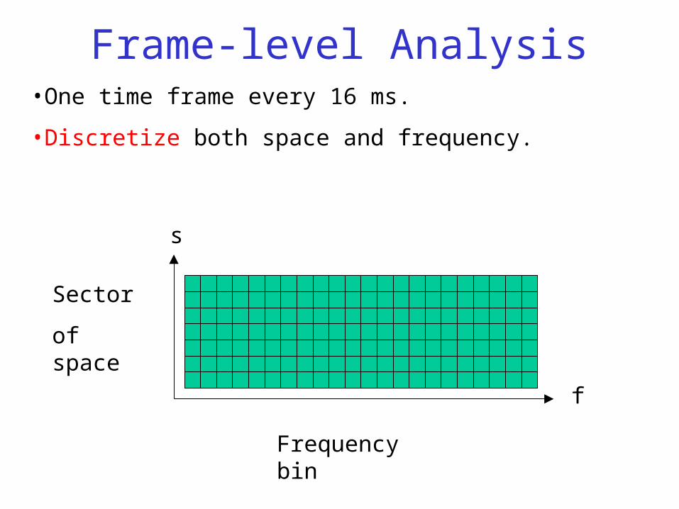
•One time frame every 16 ms.
•Discretize both space and frequency.

Frame-level Analysis
f
s
Sector
of space
Frequency bin
•One time frame every 16 ms.
•Discretize both space and frequency.
•Sparsity assumption [Roweis 03].

Frame-level Analysis
f
s
Sector
of space
Frequency bin
•One time frame every 16 ms.
•Discretize both space and frequency.
•Sparsity assumption [Roweis 03].
0
9
2
0
10
0
1

Frame-level Analysis
f
s
Sector
of space
Frequency bin
•One time frame every 16 ms.
•Discretize both space and frequency.
•Sparsity assumption [Roweis 03].
0
9
2
0
10
0
1

Frequency Bin Analysis
•Compute phase between 2 microphones: (f) in
•Repeat for all P microphone pairsf1(f) …P(f)].
P=M(M-1)/2
Frequency Bin Analysis
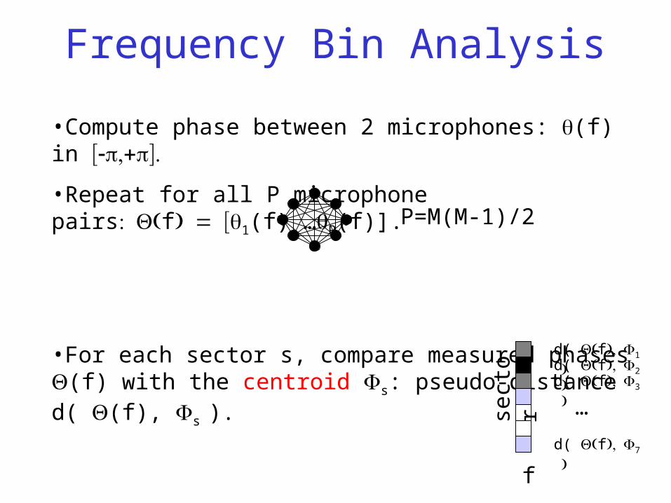
•Compute phase between 2 microphones: (f) in
•Repeat for all P microphone pairsf1(f) …P(f)].
•For each sector s, compare measured phases (f) with the centroid s: pseudo-distance d( (f), s ).
P=M(M-1)/2
sect
orf
d( f1d( f2d( f3
d( f7
…

Frequency Bin Analysis
•Compute phase between 2 microphones: (f) in
•Repeat for all P microphone pairsf1(f) …P(f)].
•For each sector s, compare measured phases (f) with the centroid s: pseudo-distance d( (f), s ).
•Apply sparsity assumption:
–The best one only is active.
P=M(M-1)/2

Outline
• Context and problem.
• Approach.– Discretize: ( sector, time frame, frequency bin ).– Example.
• Experiments.– Multiple loudspeakers.– Multiple humans.
• Conclusion.

Real Data: Single Speaker
Without sparsity assumption [SAPA 04] similar to [ICASSP 01]

Real Data: Single Speaker
With sparsity assumption (this work)
Without sparsity assumption [SAPA 04] similar to [ICASSP 01]

Outline
• Context and problem.
• Approach.– Discretize: ( sector, time frame, frequency bin ).– Example.
• Experiments.– Multiple loudspeakers.– Multiple humans.
• Conclusion.

Real Data: Multiple Loudspeakers

Task 2: Multiple Loudspeakers
Metric Ideal Result
>=1 detected 100%
Average
nb detected
2.0
2 loudspeakers simultaneously active

Real Data: Multiple Loudspeakers
Metric Ideal Result
>=1 detected 100% 100%
Average
nb detected
2.0 1.9
2 loudspeakers simultaneously active
Real Data: Multiple Loudspeakers
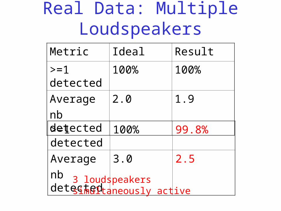
Metric Ideal Result
>=1 detected 100% 100%
Average
nb detected
2.0 1.9
>=1 detected 100% 99.8%
Average
nb detected
3.0 2.5
3 loudspeakers simultaneously active

Outline
• Context and problem.
• Approach.– Discretize: ( sector, time frame, frequency bin ).– Example.
• Experiments.– Multiple loudspeakers.– Multiple humans.
• Conclusion.

Real data: Humans

Real data: Humans
Metric Ideal Result
>=1 detected ~89.4% 90.8%
Average
nb detected
~1.3 1.3
2 speakers simultaneously active (includes short silences)

Real data: Humans
Metric Ideal Result
>=1 detected ~89.4% 90.8%
Average
nb detected
~1.3 1.3
3 speakers simultaneously active (includes short silences)
>=1 detected ~96.5% 95.1%
Average
nb detected
~2.0 1.6

Conclusion
• Sector-based approach.
• Localization and detection.
• Effective on real multispeaker data.

Conclusion
• Sector-based approach.
• Localization and detection.
• Effective on real multispeaker data.
• Current work:– Optimize centroids.– Multi-level implementation.– Compare multilevel with existing methods.
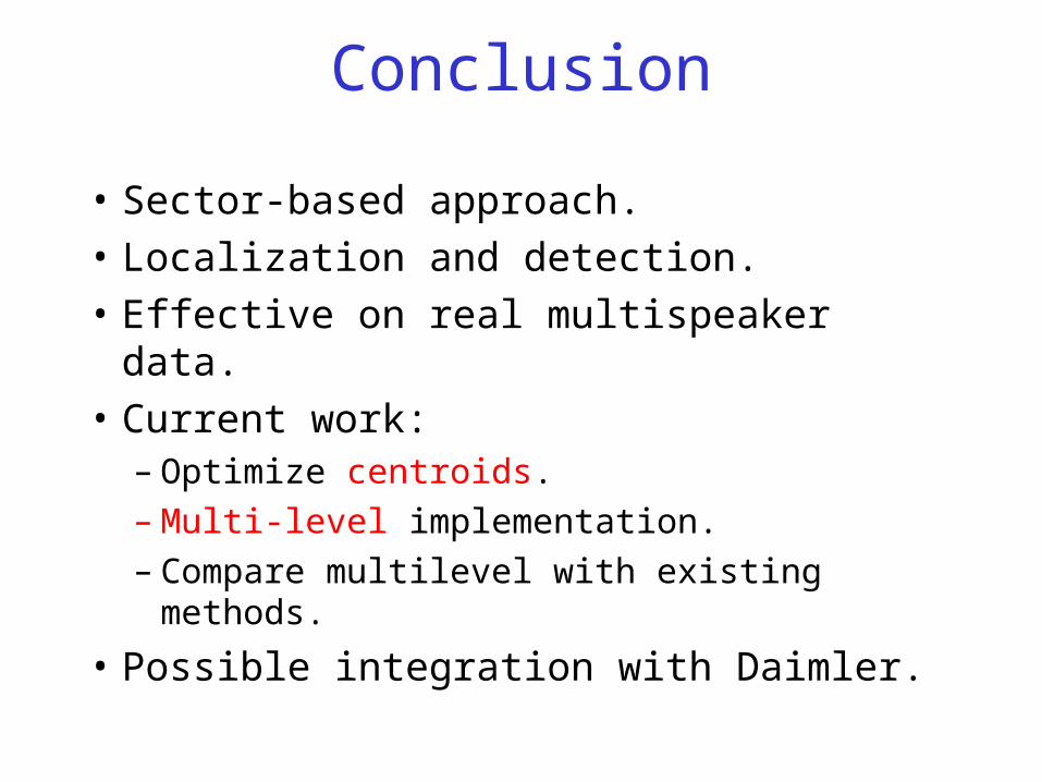
Conclusion
• Sector-based approach.
• Localization and detection.
• Effective on real multispeaker data.
• Current work:– Optimize centroids.– Multi-level implementation.– Compare multilevel with existing methods.
• Possible integration with Daimler.

Thank you!
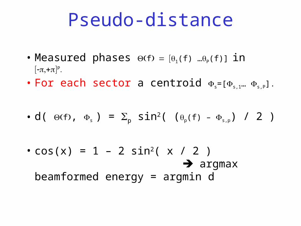
Pseudo-distance
• Measured phases f1(f) …P(f)]in P
• For each sector a centroid s=[s,1… s,P].
• d( f, s ) = p sin2( (p(f) – s,p) / 2 )
• cos(x) = 1 – 2 sin2( x / 2 ) argmax beamformed energy = argmin d

Delay-sum vs Proposed (1/3)
With optimized centroids (this work)
With delay-sum centroids (this work)

Delay-sum vs Proposed (2/3)
Metric Ideal Delay-sum Proposed
>=1 detected 100% 99.9% 100%
Average nb detected
2.0 1.8 1.9
2 loudspeakers simultaneously active
>=1 detected 100% 99.2% 99.8%
Average nb detected
3.0 1.9 2.5
3 loudspeakers simultaneously active
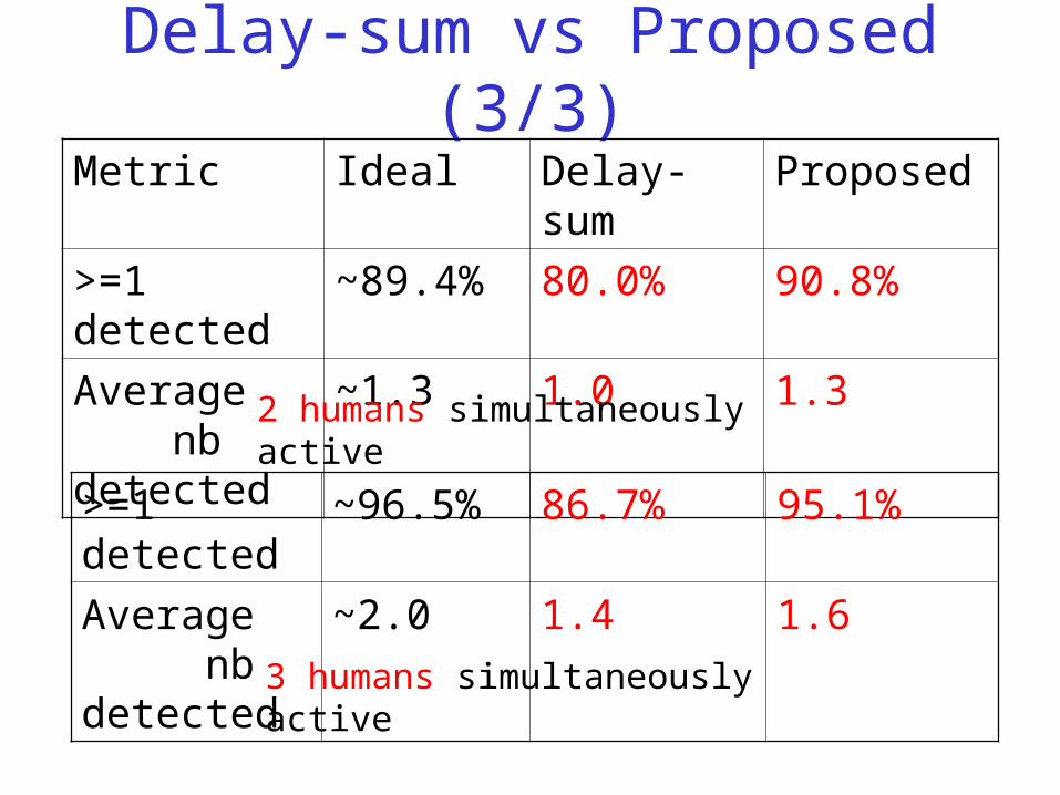
Delay-sum vs Proposed (3/3)
Metric Ideal Delay-sum Proposed
>=1 detected ~89.4% 80.0% 90.8%
Average nb detected
~1.3 1.0 1.3
2 humans simultaneously active
>=1 detected ~96.5% 86.7% 95.1%
Average nb detected
~2.0 1.4 1.6
3 humans simultaneously active

Energy and Localization