multiphase flow models in a network of pipes · networks consisting of pipelines interconnected at...
TRANSCRIPT

Introduction and motivation The drift flux multiphase model Mathematical Analysis of the fine model Coupling conditions at pipe-to-pipe intersection Numerical
Multiphase flow models in a network of pipes
Jean Medard T Ngnotchouye1 MK Banda2 M Herty3
1School of Mathematics, Statistics and Computer Sciences University of KwaZulu-Natal2Department of mathematics, University of Pretoria 3RWTH Aachen, Germany
Evolutionary processes on networksKigali, Rwanda, 20-24th March 2018
Multiphase flow models in a network of pipes JM Ngnotchouye

Introduction and motivation The drift flux multiphase model Mathematical Analysis of the fine model Coupling conditions at pipe-to-pipe intersection Numerical
Outline
1 Introduction and motivation
2 The drift flux multiphase model
3 Mathematical Analysis of the fine model
The standard Riemann problem
Semi-analytical examples
4 Coupling conditions at pipe-to-pipe intersection
5 Numerical examples
Multiphase flow models in a network of pipes JM Ngnotchouye
Introduction and motivation The drift flux multiphase model Mathematical Analysis of the fine model Coupling conditions at pipe-to-pipe intersection Numerical
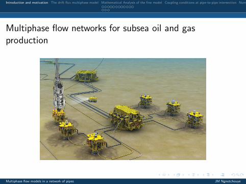
Multiphase flow networks for subsea oil and gasproduction
Multiphase flow models in a network of pipes JM Ngnotchouye

Introduction and motivation The drift flux multiphase model Mathematical Analysis of the fine model Coupling conditions at pipe-to-pipe intersection Numerical
Multiphase flow networks for subsea oil and gasproduction
Multiphase flow models in a network of pipes JM Ngnotchouye
Introduction and motivation The drift flux multiphase model Mathematical Analysis of the fine model Coupling conditions at pipe-to-pipe intersection Numerical
Multiphase flow networks for subsea oil and gasproduction
• In these networks, there is a presence of wells, collection systems,pipelines, processing units such as pumps and separators.
• Real time data capture and storage capabilities have paved the way forthe use of model-based techniques to improve operations.
• In practice, the use of model-based methods translates into advisorysystems for production engineers.
• Such systems use real-time data in combination with calibratedmathematical models and optimisation to improve the economics of an oilfield by increasing throughput.
• Some claims to a production increase of up to 4% due to the use of modelbased tools
• Grimstad et al. [Grimstad et al., 2016] propose a global optimisationmethod using spline-based surrogate model.
• Their main strategies are to adapt well-known graph based modelingscheme to oil and gas network, then use spline-based surrogate models torepresent the nonlinear parts of the system and then use a global branchand bound based optimisation solver.Multiphase flow models in a network of pipes JM Ngnotchouye

Introduction and motivation The drift flux multiphase model Mathematical Analysis of the fine model Coupling conditions at pipe-to-pipe intersection Numerical
Steady state analysis of gas network with distributed injection ofalternative gas
• Natural gas seem to be a viable alternative to curb high carbon emissionby industrialized countries.
• Steady state analysis of gas networks is usually used to compute nodalpressures and pipe flows for given values of source node pressures and gasconsumption.
• Traditional methods of modeling and simulating gas networks assume agas mixture with a uniform composition to be transported via the network
• Abeysekera et al. [Abeysekera et al., 2016] propose methods forsimulation of gas networks considering a diversity of alternative gas(hydrogen, upgraded biogas)injections.
• In their proposed method, a set of algebraic equations, equal in number tothe state variables to be calculated are formulated using the gas pipe flowequations and Kirchhoffs first law applied at nodes.
• Injection of alternative gases in a gas grid has an impact both atappliance level and at network level.
Multiphase flow models in a network of pipes JM Ngnotchouye
Introduction and motivation The drift flux multiphase model Mathematical Analysis of the fine model Coupling conditions at pipe-to-pipe intersection Numerical
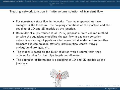
Treating network junction in finite volume solution of transient flow
• For non-steady state flow in networks. Two main approaches haveemerged in the literature: the coupling conditions at the junction and thecoupling of 1D and 2D models at the junction.
• Bermudez et al [Bermudez et al., 2017] propose a finite volume methodto solve the equations modelling the gas flow in gas transportationnetworks consisting of pipelines interconnected at nodes and some otherelements like compression stations, pressure/flow control valves,underground storages, etc.
• The model is based on the Euler equation with a source term thataccount for pipe friction, pipe length and diameter.
• The approach of Bermudez is a coupling of 1D and 2D models at thejunctions.
Multiphase flow models in a network of pipes JM Ngnotchouye

Introduction and motivation The drift flux multiphase model Mathematical Analysis of the fine model Coupling conditions at pipe-to-pipe intersection Numerical
A review of multiphase models in networks
• In the past, analysis of two-phase flow pipelines in the petroleumindustry were performed primarily with the use of steady-statemethods.
• However, various operational events such as flow rate changes,shutdowns-restarts, and pipeline leaks cause unsteady flow. Clearly,steady-state methods can not be applied to perform analysis underthese circumstances and transient two-phase flow calculations shouldbe used.
• Multiphase flow is a phase in which natural gas is found in theprocess of oil recovery from the reservoir.
• The reservoir contains in general a large quantity of methane alongwith heavier hydrocarbons such as ethane, propane, isobutane,normal butane, etc.
• It is also generally saturated with water.
Multiphase flow models in a network of pipes JM Ngnotchouye

Introduction and motivation The drift flux multiphase model Mathematical Analysis of the fine model Coupling conditions at pipe-to-pipe intersection Numerical
The drift-flux model
• We consider a non-isothermal transient two-phase model in a pipewith the assumptions that the amount of liquid is small and the gasflow rate is high with both the gas and liquid phases obeying thelaws of continuum mechanics,
• the liquid droplet are assumed to have uniform size,
• the flow is assumed to be one-dimensional in the axial direction ofthe pipe and the diameter of the pipe is assumed to be constantalong the pipe,
• gas and liquid phases are assumed to be at local equilibrium at everypoint within the pipe,
• dissipation and compression terms are neglected and there is nocoagulation, nor agglomeration [Dukhovnaya and Adewumi, 2000].
Multiphase flow models in a network of pipes JM Ngnotchouye

Introduction and motivation The drift flux multiphase model Mathematical Analysis of the fine model Coupling conditions at pipe-to-pipe intersection Numerical
Problem formulation
• The governing equations can be written in conservative form as
∂U
∂t+
∂f (U)
∂x= G(U) (1)
where
U =
ρg
ρl
mg
ml
Hg
Hl
; f (U) =
mg
ml
m2g
ρg+ c2
gρg
m2l
ρl+ c2
l ρl
Hgmg
ρg
Hlml
ρl
; G(U) =
Mgl
Mlg
−∑
Fig − αggg sin θ
−∑
Fil − αllg sin θ
Qg + hgl + hg
Ql + hlg + hl
(2)
Multiphase flow models in a network of pipes JM Ngnotchouye

Introduction and motivation The drift flux multiphase model Mathematical Analysis of the fine model Coupling conditions at pipe-to-pipe intersection Numerical
Problem formulation
• These equations are derived from the continuity equations, themomentum equations and the energy equations under theassumptions that the rate of change of the volume fractions αg andαl with respect to the flow direction are sufficiently small and thatthe sound speeds cg and cl are constant along the flow direction.
• The conservative variables are related to the primal variable throughthe relationships
ρg = gαg ρl = lαl ,
mg = gαgvg ml = lαlvl ,
Hg = gαg Hg Hl = lαl Hl .
(3)
g ,l , vg ,l and Hg ,l are the densities, velocity and enthalpy of the gasand liquid phases, respectively.
Multiphase flow models in a network of pipes JM Ngnotchouye

Introduction and motivation The drift flux multiphase model Mathematical Analysis of the fine model Coupling conditions at pipe-to-pipe intersection Numerical
Problem formulation• We note that the two phases fill the entire pipe:
αg + αl = 1.
• The mass transfer rate experienced by the gas and liquid phases areequal in magnitude but of opposite sign:
Mgl = −Mlg .
• The drag forces and mass transfer forces exerted on one phase bythe other are equal but of opposite sign:
Fdg = −Fdl , Fmg = −Fml .
• The energy transfer rate from one phase to another are equal andthe rate of change of latent heat from one phase to another areequal but of opposite sign:
hgl = −hlg , hg = −hl .
Multiphase flow models in a network of pipes JM Ngnotchouye

Introduction and motivation The drift flux multiphase model Mathematical Analysis of the fine model Coupling conditions at pipe-to-pipe intersection Numerical
Problem formulation
• The frictional force between each phase and the pipe wall isdetermined using volume-fraction-modified form of the single phaseflow model. The mixture properties in the single-phase model arereplaced with the phasic properties. For gas and liquid phases thefrictional forces are written as:
Fwg =αg fggvg |vg |
2d
Fwl =αl fllvl |vl |
2d
• where fg and fl are Darcy’s friction factors for gas and liquid phases,respectively. These are calculated using Chen’s equation
Multiphase flow models in a network of pipes JM Ngnotchouye

Introduction and motivation The drift flux multiphase model Mathematical Analysis of the fine model Coupling conditions at pipe-to-pipe intersection Numerical
An hierarchy of models related to the drift-flux model
• Following [Domschke et al., 2018] we define an hierachy of modelsderived from the drift-flux model
• For the first simplified model, we assume that the velocity andpressure of the two phases are equal and that the source term iszero. We then obtain the no-slip drift-flux model[Banda et al., 2010b]in conservative form
∂tρ1 + ∂xρ1Iρ
= 0;
∂tρ2 + ∂xρ2Iρ
= 0;
∂t I + ∂x
(
ρ(u2 + a2
2))
= 0;
(4)
where ρ = ρ1 + ρ2, I = ρu.
Multiphase flow models in a network of pipes JM Ngnotchouye

Introduction and motivation The drift flux multiphase model Mathematical Analysis of the fine model Coupling conditions at pipe-to-pipe intersection Numerical
An hierarchy of models related to the drift-flux model
• At the next approximation, we assume that the sonic speed of thetwo phases are different. This gives the simplified model[Banda et al., 2010a]
∂tρ1 + ∂xρ1Iρ
= 0
∂tρ2 + ∂xρ2Iρ
= 0
∂t I + ∂x
(
I 2
ρ+ ρ1a
21 + ρ2a
22
)
= 0
(5)
where we have taken I = ρu, ρ = ρ1 + ρ2.
• At the next level, we assume that the pressure p(ρ1, ρ2) is as generalas possible.
• This model was analyzed in [Banda et al., 2015] using the idea oflinearisation of the Lax curve.
Multiphase flow models in a network of pipes JM Ngnotchouye

Introduction and motivation The drift flux multiphase model Mathematical Analysis of the fine model Coupling conditions at pipe-to-pipe intersection Numerical
The corresponding conservation law problem
• The equation (1) can be written in quasi-linear form as
Ut + A(U)Ux = H(U), (6)
where A(U) is the Jacobian matrix of the flux function f evaluatedas
A(U) =
0 0 1 0 0 00 0 0 1 0 0
c2g − v2
g 0 2v2g 0 0 0
0 c2l − v2
l 0 2v2l 0 0
−vgHg 0 Hg 0 vg 00 −vlHl 0 Hl 0 vl
Multiphase flow models in a network of pipes JM Ngnotchouye

Introduction and motivation The drift flux multiphase model Mathematical Analysis of the fine model Coupling conditions at pipe-to-pipe intersection Numerical
Problem formulation
• The eigenvalues of matrix A(U) are:
λ1 = vg − cg ; λ2 = vg ; λ3 = vg + cg ;λ4 = vl − cl ; λ5 = vl ; λ6 = vl + cl .
(7)
• with the corresponding right eigenvectors
r1 =
10
vg − cg
0Hg
0
; r2 =
0000
Hg
0
; r3 =
10
vg + cg
0Hg
0
; (8)
Multiphase flow models in a network of pipes JM Ngnotchouye

Introduction and motivation The drift flux multiphase model Mathematical Analysis of the fine model Coupling conditions at pipe-to-pipe intersection Numerical
Problem formulation
• and
r4 =
010
vl − cl
0Hl
; r5 =
00000Hl
r6 =
010
vl + cl
0Hl
. (9)
Multiphase flow models in a network of pipes JM Ngnotchouye

Introduction and motivation The drift flux multiphase model Mathematical Analysis of the fine model Coupling conditions at pipe-to-pipe intersection Numerical
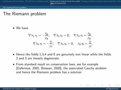
The standard Riemann problem
The Riemann problem
• We have
∇λ1 r1 = − cg
ρg
; ∇λ2 r2 = 0; ∇λ3 r3 =cg
ρg
;
∇λ4 r4 = − cl
ρl
; ∇λ5 r5 = 0; λ6 r6 =cl
ρl
.
• Hence the fields 1,3,4 and 6 are genuinely non linear while the fields2 and 5 are linearly degenerate.
• From standard result on conservation laws, see for example[Dafermos, 2005, Bressan, 2000], the associated Cauchy problemand hence the Riemann problem has a solution.
Multiphase flow models in a network of pipes JM Ngnotchouye
Introduction and motivation The drift flux multiphase model Mathematical Analysis of the fine model Coupling conditions at pipe-to-pipe intersection Numerical
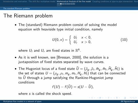
The standard Riemann problem
The Riemann problem
• The (standard) Riemann problem consist of solving the modelequation with heaviside type initial condition, namely
U(0, x) =
{
Ul x < 0,
Ur x > 0,(10)
where Ul and Ur are fixed states in R6.
• As it is well known, see [Bressan, 2000], the solution is ajuxtaposition of fixed states separated by wave curves.
• The Hugoniot locus of a fixed state U = (ρg , ρl , mg , ml , Hg , Hl) isthe set of states U = (ρg , ρl , mg , ml , Hg , Hl) that can be connectedto U through a jump satisfying the Rankine-Hugoniot jumpconditions
f (U) − f (U) = s(U − U),
where s is called the shock speed.
Multiphase flow models in a network of pipes JM Ngnotchouye
Introduction and motivation The drift flux multiphase model Mathematical Analysis of the fine model Coupling conditions at pipe-to-pipe intersection Numerical
The standard Riemann problem
The Riemann problem
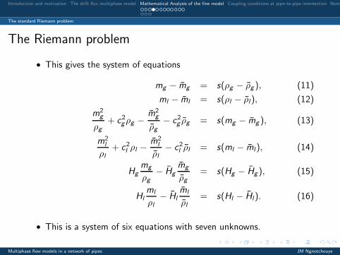
• This gives the system of equations
mg − mg = s(ρg − ρg ), (11)
ml − ml = s(ρl − ρl), (12)
m2g
ρg
+ c2gρg −
m2g
ρg
− c2g ρg = s(mg − mg ), (13)
m2l
ρl
+ c2l ρl −
m2l
ρl
− c2l ρl = s(ml − ml), (14)
Hg
mg
ρg
− Hg
mg
ρg
= s(Hg − Hg ), (15)
Hl
ml
ρl
− Hl
ml
ρl
= s(Hl − Hl). (16)
• This is a system of six equations with seven unknowns.
Multiphase flow models in a network of pipes JM Ngnotchouye

Introduction and motivation The drift flux multiphase model Mathematical Analysis of the fine model Coupling conditions at pipe-to-pipe intersection Numerical
The standard Riemann problem
The Riemann problem• Solving for the variables ρl , mg , ml , Hg , Hl and s in terms of ρg
gives the 1-3 shock curves as
S1,3(ξ; U) : ξ 7→
ρgξ
ρl
c2l
(
mg
ρg− ml
ρl∓ cg
√ξ)2
mgξ ∓ cg ρg
√ξ(ξ − 1)
ml + (mg
ρg∓ cg
√ξ)
[
ρl
c2l
(
mg
ρg− ml
ρl∓ cg
√ξ)2
− ρl
]
Hgξ
Hl
mlρl
− mgρg
±cg
√ξ
mlρl
− mgρg
±cg√
ξ
.
(17)
• The shock speeds associated with the 1 and 3-fields are
s1,3 =mg
ρg
∓ cg
√
ρg
ρg
. (18)
Multiphase flow models in a network of pipes JM Ngnotchouye

Introduction and motivation The drift flux multiphase model Mathematical Analysis of the fine model Coupling conditions at pipe-to-pipe intersection Numerical
The standard Riemann problem
The Riemann problem• Similarly, the 4-6 shock curves can also be found as
S4,6(ξ; U) : ξ 7→
ρg
c2g
(
ml
ρl− mg
ρg∓ cl
√ξ)2
ρlξ
mg + ( ml
ρl∓ cl
√ξ)
[
ρg
c2g
(
ml
ρl− mg
ρg∓ cl
√ξ)2
− ρg
]
mlξ ∓ cl ρl
√ξ(ξ − 1)
Hg
mgρg
− mlρl
±cl
√ξ
mgρg
− mgρg
±cg√
ξ
Hlξ
.
(19)
• with the corresponding shock speed as
s4,6 =ml
ρl
∓∣
∣
∣
∣
mg
ρg
∓ cg
√
ρg
ρg
− ml
ρl
∣
∣
∣
∣
. (20)
Multiphase flow models in a network of pipes JM Ngnotchouye

Introduction and motivation The drift flux multiphase model Mathematical Analysis of the fine model Coupling conditions at pipe-to-pipe intersection Numerical
The standard Riemann problem
The Riemann problem
• The admissible, in the sense of Lax, forward 1,4-shock and 3,6-shockwaves satisfy ξ > 1 and ξ < 1, respectively while the backward shockwaves satisfy the reverses inequalities.
• The rarefaction curves are found as the integral curves of the eigenvectorsof the flux function.
• Their expression are found by solving the ordinary differential equation
d
dτU =
ri(U)
∇λi (U) · ri (U), U(0) = U. (21)
• The solution of the ODE (21) gives the 1 and 3-rarefaction curves as
R1(ξ; U) : ξ 7→
2
6
6
6
6
6
6
4
ρgξρl
(mg − cg ρg ln ξ)ξml
HgξHl
3
7
7
7
7
7
7
5
; R3(ξ; U) : ξ 7→
2
6
6
6
6
6
6
4
ρgξρl
(mg + cg ρg ln ξ)ξml
HgξHl
3
7
7
7
7
7
7
5
.
(22)
Multiphase flow models in a network of pipes JM Ngnotchouye

Introduction and motivation The drift flux multiphase model Mathematical Analysis of the fine model Coupling conditions at pipe-to-pipe intersection Numerical
The standard Riemann problem
The Riemann problem
• Similarly, the 4 and 6 -rarefaction curves are given by
R4(ξ; U) : ξ 7→
2
6
6
6
6
6
6
4
ρg
ρlξmg
(ml − cl ρl ln ξ)ξHg
Hlξ
3
7
7
7
7
7
7
5
; R6(ξ; U) : ξ 7→
2
6
6
6
6
6
6
4
ρg
ρlξmg
(ml + cl ρl ln ξ)ξHg
Hlξ
3
7
7
7
7
7
7
5
.
(23)
• Along the contact discontinuities, only the enthalpy changes and weobtain the contact discontinuity wave curves as
L2(ξ; U) : ξ 7→
2
6
6
6
6
6
6
6
4
ρg
ρl
mg
ml
Hg
ρgξ
Hl
3
7
7
7
7
7
7
7
5
; L5(ξ; U) : ξ 7→
2
6
6
6
6
6
6
4
ρg
ρl
mg
ml
Hg
Hl
ρlξ
3
7
7
7
7
7
7
5
. (24)
Multiphase flow models in a network of pipes JM Ngnotchouye

Introduction and motivation The drift flux multiphase model Mathematical Analysis of the fine model Coupling conditions at pipe-to-pipe intersection Numerical
The standard Riemann problem
The Riemann problem• A typical solution to the Riemann problem has the wave structure
depicted in the figure below
x
t
Ul
U1
U2
U3
U4U5
UR
Figure: A typical solution to the standard Riemann problem
• therein, the dotted line represent a contact discontinuity curve, thefan represent the rarefaction curve and the thick solid line representa shock curve.
Multiphase flow models in a network of pipes JM Ngnotchouye

Introduction and motivation The drift flux multiphase model Mathematical Analysis of the fine model Coupling conditions at pipe-to-pipe intersection Numerical
The standard Riemann problem
The Riemann problem
• In this case the intermediary states are worked out as
U1 = L+1 (ξ1, Ul), U2 = L2(ξ2, U1), U3 = L+
3 (ξ3, U2),U4 = L+
4 (ξ4, U3), U5 = L5(ξ5, U4), U6 = L+6 (ξ6, U5).
(25)
• The parameter ξ = (ξ1, ξ2, ξ3, ξ4, ξ5, ξ6) are obtained by solving theequation
U6 − Ur = 0 (26)
for ξ.
• We solve below this nonlinear equation numerically using theNewton’s method.
Multiphase flow models in a network of pipes JM Ngnotchouye

Introduction and motivation The drift flux multiphase model Mathematical Analysis of the fine model Coupling conditions at pipe-to-pipe intersection Numerical
The standard Riemann problem
The Riemann problem• We depict below a projection of the forward 1,3-waves curves in the
ρg − mg plane and the projection of the forward 4-6 wave curves inthe ρl − ml plane for a fixed state
U =[
1.0 0.11 2.5 1.2 45.0 11.0]T
.
0 0.2 0.4 0.6 0.8 1 1.2 1.4 1.6 1.8 2−80
−60
−40
−20
0
20
40
60
80
100
ρg
mg
forward 1−3lax curves
Forward S1Forward R1Forward S3Forward R3
0 0.05 0.1 0.15 0.2 0.25−10
−5
0
5
10
15
ρl
ml
forward 4−6lax curves
Forward S4Forward R4Forward S6Forward R6
Figure: 1,3-forward Lax curves for the multiphase model in the ρg − mg
plane (left) and 4,6-forward Lax curves for the multiphase model in theρl − ml plane.
Multiphase flow models in a network of pipes JM Ngnotchouye

Introduction and motivation The drift flux multiphase model Mathematical Analysis of the fine model Coupling conditions at pipe-to-pipe intersection Numerical
The standard Riemann problem
The Riemann problem
Theorem[Bressan, 2000]
For ‖Ur − Ul‖ sufficiently small, there exists a unique self similar solutionto the Riemann problem (1,10) with small total variation. The solutioncomprises 7 constant states U0 = Ul , U1, . . . , U6 = U r . When the i-thcharacteristic field is linearly degenerate, Ui is joined to Ui−1 by ani-contact discontinuity curve, while when the i-characteristic field isgenuinely nonlinear, Ui is joined to Ui−1 by either an i-(Lax) rarefactionor an i-(Lax) shock curve.
Multiphase flow models in a network of pipes JM Ngnotchouye

Introduction and motivation The drift flux multiphase model Mathematical Analysis of the fine model Coupling conditions at pipe-to-pipe intersection Numerical
Semi-analytical examples
A Numerical example
• We consider an example where the Riemann problem is solvedexactly as in Theorem above. We will describe the qualitativebehavior of the solution by writing for exampleS1 − C2 −R3 −S4 − C5 −S6 to signify that the solution has a shockwave in the 1−field, a contact discontinuity in the 2−field, ararefaction wave in the 3−field, a shock wave in the 4−field, acontact discontinuity in the 5−field and a shock wave in the 6−field.
• In the first example we consider a multiphase flow with the soundspeeds cg = 30.5000 and cl = 100.5
Multiphase flow models in a network of pipes JM Ngnotchouye

Introduction and motivation The drift flux multiphase model Mathematical Analysis of the fine model Coupling conditions at pipe-to-pipe intersection Numerical
Semi-analytical examples
A Numerical example
• The initial conditions are given in the table below. Note that in thisexample the mixture is at rest at the initial time on both sides of themembrane.
ρg ρl mg ml Hg Hl
Ul 15.5000 1.0000 0.0000 0.0000 5.0000 11.0000Ur 10.6000 1.1000 0.000 0.000 4.0000 10.8000
The intermediary states are presented in the next slide. Thequalitative behavior of the solution is of the formS1 − C2 − S3 − S4 − C5 −R6.
Multiphase flow models in a network of pipes JM Ngnotchouye

Introduction and motivation The drift flux multiphase model Mathematical Analysis of the fine model Coupling conditions at pipe-to-pipe intersection Numerical
Semi-analytical examples
A Numerical example
• Solution of the previous example
ρg ρl mg ml Hg Hl
Ul 15.5000 1.0000 0.0000 0.0000 5.0000 11.0000U1 80.6 0.5 -4528.9 36.2 26.0 5.3U2 80.6 0.5 -4528.9 36.2 30.4 5.3U3 64.6 0.5 -4.0668 35.1 24.4 5.7U4 10.6000 1.0498 0.00 -4.9250 4.0000 11.5482U5 10.6000 1.0498 0.00 -4.9250 4.0000 10.3075Ur 10.6000 1.1000 0.0000 0.0000 4.0000 10.8000
Multiphase flow models in a network of pipes JM Ngnotchouye
Introduction and motivation The drift flux multiphase model Mathematical Analysis of the fine model Coupling conditions at pipe-to-pipe intersection Numerical
A model for the network of pipes
• The network of pipes is considered as a oriented graph (P ,V) wherethe edges P of the graph represent the pipes and the nodes Vrepresent the junctions.
• Each pipe j ∈ P is parametrised by an interval Ij.= [xa
j , xbj ].
• Each node of the graph correspond to a junction of pipes. Forv ∈ V , the set of pipe j ∈ P ingoing to v are denoted as δ−v and theset of outgoing pipes are denoted as δ+
v .
• The set of all the pipes meeting at the junction v is denoted asδv = δ−v ∪ δ+
v . We will call the cardinality of the set δv the degree ofthe junction v .
Multiphase flow models in a network of pipes JM Ngnotchouye

Introduction and motivation The drift flux multiphase model Mathematical Analysis of the fine model Coupling conditions at pipe-to-pipe intersection Numerical
A model for the network of pipes
1
2
3
n
n + 1
n + 2
p
δ−v
δ+v
v
Figure: A junction with n ingoing pipes and p − n outgoing pipes.
Multiphase flow models in a network of pipes JM Ngnotchouye

Introduction and motivation The drift flux multiphase model Mathematical Analysis of the fine model Coupling conditions at pipe-to-pipe intersection Numerical
A model for the flow in a network of pipes
• We assume that for each pipe j ∈ P , the flow is governed by theequation (4) rewritten as
∂U j
∂t+
∂f (U j)
∂x= 0, U j =
ρj1
ρj2
I j
, (27)
where the flux function is given either by (1), (4) or (5).
• The Riemann problem at the junction assumed for the analysis atv = 0 consists of solving the flow equations in all the pipes j ∈ δv
with constant initial data in each pipe
U j(0±, x) = U j , x ja ≤ x ≤ x
jb, (28)
and with some coupling conditions at the junction v describing theinteraction of the flow at the junction. These coupling conditionsprovide for the simulations as boundary conditions at the interiornodes of each pipe.
Multiphase flow models in a network of pipes JM Ngnotchouye

Introduction and motivation The drift flux multiphase model Mathematical Analysis of the fine model Coupling conditions at pipe-to-pipe intersection Numerical
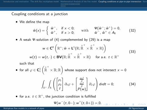
Coupling conditions at a junction
• For simplicity we consider the case of a junction with only two pipes,one ingoing and one outgoing. The result can be extended tojunctions with higher degree in a straightforward way.
• At the junction, located at x = 0, the dynamics are governed by thecoupling conditions
Ψ(
w−(t, 0−); w+(t, 0+))
= 0, (29)
where the w− and w+ are the flow variables in the left and rightpipe, respectively.
• The subsonic region is defined as
A0 = {w ∈◦
R
+
×◦
R
+
× R : λ1(w) < 0 < λ2(w) < λ3(w)}. (30)
• For later use, we define the quantities
M(w) =ρ1I
ρ1 + ρ2
, N(w) =ρ2I
ρ1 + ρ2
, P(w) =I 2
ρ1 + ρ2
+ p(ρ1, ρ2).
(31)
Multiphase flow models in a network of pipes JM Ngnotchouye
Introduction and motivation The drift flux multiphase model Mathematical Analysis of the fine model Coupling conditions at pipe-to-pipe intersection Numerical
Coupling conditions at a junction
• We define the map
w(x) =
w−, if x < 0;w+, if x > 0;
withΨ(w−; w+) = 0,w−, w+ ∈ A0
(32)
• A weak Ψ-solution of (4) complemented by (29) is a map
w ∈ C0
„
R+; w + L
1(R;◦
R
+
×◦
R
+
× R)
«
w(t) = w(t, ·) ∈ BV(R;◦
R
+
×◦
R
+
× R) for a.e. t ∈ R+
(33)
such that
• for all ϕ ∈ C1c
„
◦
R
+
× R; R
«
whose support does not intersect x = 0
Z
R+
Z
R
0
@
2
4
ρ1
ρ2
I
3
5 ∂tϕ +
2
4
ρ1I
ρ
ρ1I
ρ
P(w)
3
5 ∂xϕ
1
A dxdt = 0; (34)
• for a.e. t ∈ R+, the junction condition is fulfilled
Ψ(w−(t, 0−);w+(t, 0+)) = 0.
Multiphase flow models in a network of pipes JM Ngnotchouye

Introduction and motivation The drift flux multiphase model Mathematical Analysis of the fine model Coupling conditions at pipe-to-pipe intersection Numerical
Coupling conditions at a junction
• Consider now the coupling conditions
Ψ(
w−; w+)
=
M(w+) − M(w−)N(w+) − N(w−)P(w+) − P(w−)
. (35)
• This amounts to the conservation of mass of each phase and theequality of the dynamic pressure at the junction.
• It can be shown that using (35) a solution is equivalent to theclassical solution of the Riemann problem on R with initial data in aneighborhood of a subsonic state w .
• In general, the existence of the solution to the Riemann problem atthe junction is proven by exhibiting some intermediary states thatcouples the flow at the junction though the Lax curves.
Multiphase flow models in a network of pipes JM Ngnotchouye

Introduction and motivation The drift flux multiphase model Mathematical Analysis of the fine model Coupling conditions at pipe-to-pipe intersection Numerical
Coupling conditions at a junction
• For a junction with m ingoing pipes and p outgoing pipes with the flowvariables in those pipes denoted by wj , j = 1, . . . m + p, we adopt thefollowing coupling condition map
Ψ(w1, . . . , wm, wm+1, . . . , wm+p) =0
B
B
B
B
B
B
B
B
B
B
B
B
B
B
B
B
B
B
@
mP
i=1
M(wi (t, 0−)) =p
P
i=1
M(wm+i (t, 0+))
mP
i=1
N(wi (t, 0−)) =p
P
i=1
N(wm+i (t, 0+))
P(w1(t, 0−)) = P(w2(t, 0−))...
P(wm−1(t, 0−)) = P(wm(t, 0−))P(wm(t, 0−)) = P(wm+1(t, 0+))
P(wm+1(t, 0+)) = P(wm+2(t, 0+))...
P(wm+p−1(t, 0+)) = P(wm+p(t, 0+))
1
C
C
C
C
C
C
C
C
C
C
C
C
C
C
C
C
C
C
A
.
Multiphase flow models in a network of pipes JM Ngnotchouye
Introduction and motivation The drift flux multiphase model Mathematical Analysis of the fine model Coupling conditions at pipe-to-pipe intersection Numerical
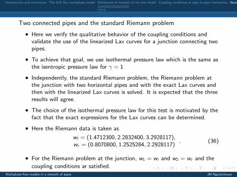
Two connected pipes and the standard Riemann problem
• Here we verify the qualitative behavior of the coupling conditions andvalidate the use of the linearized Lax curves for a junction connecting twopipes.
• To achieve that goal, we use isothermal pressure law which is the same asthe isentropic pressure law for γ = 1
• Independently, the standard Riemann problem, the Riemann problem atthe junction with two horizontal pipes and with the exact Lax curves andthen with the linearized Lax curves is solved. It is expected that the threeresults will agree.
• The choice of the isothermal pressure law for this test is motivated by thefact that the exact expressions for the Lax curves can be determined.
• Here the Riemann data is taken as
wl = (1.4712300, 2.2832400, 3.2928117),wr = (0.8070800, 1.2525284, 2.2928117)
. (36)
• For the Riemann problem at the junction, w1 = wl and w2 = wr and the
coupling conditions ar satisfied.
Multiphase flow models in a network of pipes JM Ngnotchouye

Introduction and motivation The drift flux multiphase model Mathematical Analysis of the fine model Coupling conditions at pipe-to-pipe intersection Numerical
Two connected pipes and the standard Riemann problem
• rRP is the quantity r computed as the solution of the standardRiemann problem and rCP be the same quantity computed as thesolution of the Riemann problem at the junction of two coupledpipes.
Mesh size (N) ‖IRP − ICP‖L2 ‖pRP − pCP‖L2 ‖IRP − ICP‖L2
100 1.6339e-06 1.8844e-06 0.0012
200 3.7917e-07 2.7096e-07 5.9362e-04
400 8.5111e-08 5.1969e-08 3.0193e-04
Table: L2 error in the momentum and pressure for the solution of thestandard Riemann problem and the Riemann problem at the junction
Multiphase flow models in a network of pipes JM Ngnotchouye

Introduction and motivation The drift flux multiphase model Mathematical Analysis of the fine model Coupling conditions at pipe-to-pipe intersection Numerical
Two connected pipes and the standard Riemann problem
• Now an example with the isentropic pressure law is considered. Hereγ = 5/3 is used and the following data
w1 = (1.81832, 1.44174, −0.751082), w2 = (2.01667, 1.22004, −1.584711)(37)
Mesh size (N) ‖ICP − ICPL‖L2 ‖pCP − pCPL‖L2 ‖ICP − ICPL‖L2
100 1.2886e-05 5.4828e-06 0.0038
200 3.0500e-06 1.2959e-06 0.0011
400 1.0113e-06 4.3049e-07 0.0012
Table: L2 error in the momentum and pressure for the solution of theRiemann problem at the junction with exact Lax curves and linearised Laxcurves computed for the problem in example 1
Multiphase flow models in a network of pipes JM Ngnotchouye

Introduction and motivation The drift flux multiphase model Mathematical Analysis of the fine model Coupling conditions at pipe-to-pipe intersection Numerical
Two connected pipes and the standard Riemann problem
−1 −0.8 −0.6 −0.4 −0.2 0 0.2 0.4 0.6 0.8 11.8
1.85
1.9
1.95
2
2.05
x
ρ 1
InitialStd. RPCoupled
−1 −0.8 −0.6 −0.4 −0.2 0 0.2 0.4 0.6 0.8 1
1.25
1.3
1.35
1.4
1.45
1.5
1.55
1.6
x
ρ 2
InitialStd. RPCoupled
−1 −0.8 −0.6 −0.4 −0.2 0 0.2 0.4 0.6 0.8 1−2
−1.8
−1.6
−1.4
−1.2
−1
−0.8
−0.6
x
Mom
entu
m (
I)
InitialStd. RPCoupled
−1 −0.8 −0.6 −0.4 −0.2 0 0.2 0.4 0.6 0.8 154
55
56
57
58
59
60
61
62
x
Pres
sure
(p)
InitialStd. RPCoupled
Figure: Profiles of the densities ρ1 and ρ2, the momentum I , the commonpressure p for the solution of standard Riemann problem (continuous line) andthe Riemann problem at the junction with the use of the linearized Lax curves(crosses).
Multiphase flow models in a network of pipes JM Ngnotchouye

Introduction and motivation The drift flux multiphase model Mathematical Analysis of the fine model Coupling conditions at pipe-to-pipe intersection Numerical
A junction with one ingoing and two outgoing pipes
• The initial data in the pipes are taken as
w1 = (3.4500000, 2.4050000, 6.5056726);w2 = (2.1300000, 4.1578000, 3.5720977);w3 = (2.2534000, 2.4191412, 2.9335749).
(38)
−1−0.8
−0.6−0.4
−0.20 0
0.02
0.04
0.06
0.082
2.5
3
3.5
4
tx
ρ 11
00.2
0.40.6
0.81 0
0.02
0.04
0.06
0.081.6
1.8
2
2.2
2.4
tx
ρ 12
00.2
0.40.6
0.80.02
0.04
0.06
0.081.6
1.8
2
2.2
2.4
2.6
ρ 13
Multiphase flow models in a network of pipes JM Ngnotchouye

Introduction and motivation The drift flux multiphase model Mathematical Analysis of the fine model Coupling conditions at pipe-to-pipe intersection Numerical
A junction with one ingoing and two outgoing pipes
−1−0.8
−0.6−0.4
−0.20 0
0.02
0.04
0.06
0.081.6
1.8
2
2.2
2.4
2.6
tx
ρ 21
00.2
0.40.6
0.81 0
0.02
0.04
0.06
0.083.2
3.4
3.6
3.8
4
4.2
tx
ρ 22
00.2
0.40.6
0.81 0
0.02
0.04
0.06
0.081.6
1.8
2
2.2
2.4
2.6
tx
ρ 23
Multiphase flow models in a network of pipes JM Ngnotchouye

Introduction and motivation The drift flux multiphase model Mathematical Analysis of the fine model Coupling conditions at pipe-to-pipe intersection Numerical
A junction with one ingoing and two outgoing pipes
−1−0.8
−0.6−0.4
−0.20 0
0.02
0.04
0.06
0.0880
100
120
140
160
tx
p1
00.2
0.40.6
0.81 0
0.02
0.04
0.06
0.0860
70
80
90
100
tx
p2
00.2
0.40.6
0.81 0
0.02
0.04
0.06
0.0850
60
70
80
90
tx
p3
Multiphase flow models in a network of pipes JM Ngnotchouye
Introduction and motivation The drift flux multiphase model Mathematical Analysis of the fine model Coupling conditions at pipe-to-pipe intersection Numerical
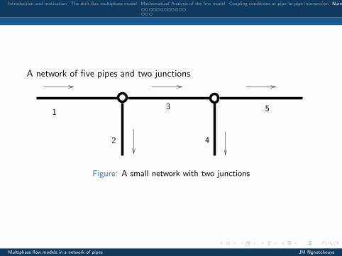
A network of five pipes and two junctions
1
2
3
4
5
Figure: A small network with two junctions
Multiphase flow models in a network of pipes JM Ngnotchouye

Introduction and motivation The drift flux multiphase model Mathematical Analysis of the fine model Coupling conditions at pipe-to-pipe intersection Numerical
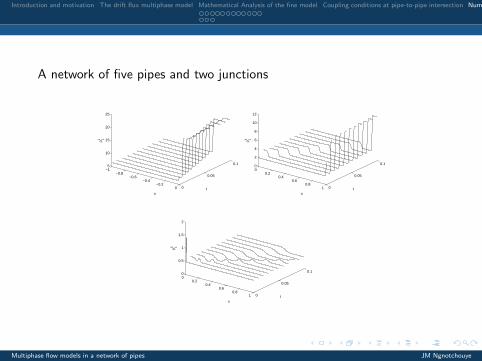
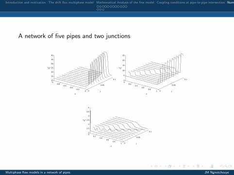
A network of five pipes and two junctions
• We consider the linear pressure law given by p = a1ρ1 + a2ρ2 witha1 = 16 and a2 = 1. The initial conditions in the pipes are given as
w1 = (6.4500, 12.8050, 31.9713);w2 = (10.3300, 3.3578, 2.4903);w3 = (1.9534, 4.5682, 29.4810);w4 = (9.0330, 18.3578, 13.0370);w5 = (0.4644, 1.2210, 16.4441).
Multiphase flow models in a network of pipes JM Ngnotchouye
Introduction and motivation The drift flux multiphase model Mathematical Analysis of the fine model Coupling conditions at pipe-to-pipe intersection Numerical
A network of five pipes and two junctions
−1−0.8
−0.6−0.4
−0.20 0
0.05
0.15
10
15
20
25
tx
ρ 11
00.2
0.40.6
0.81 0
0.05
0.10
2
4
6
8
10
12
tx
ρ 13
00.2
0.40.6
0.81 0
0.05
0.10
0.5
1
1.5
2
tx
ρ 15
Multiphase flow models in a network of pipes JM Ngnotchouye
Introduction and motivation The drift flux multiphase model Mathematical Analysis of the fine model Coupling conditions at pipe-to-pipe intersection Numerical
A network of five pipes and two junctions
−1−0.8
−0.6−0.4
−0.20 0
0.05
0.110
15
20
25
30
35
40
tx
ρ 21
00.2
0.40.6
0.81 0
0.05
0.10
5
10
15
20
25
tx
ρ 23
00.2
0.40.6
0.81 0
0.05
0.11
1.5
2
2.5
3
3.5
4
tx
ρ 25
Multiphase flow models in a network of pipes JM Ngnotchouye

Introduction and motivation The drift flux multiphase model Mathematical Analysis of the fine model Coupling conditions at pipe-to-pipe intersection Numerical
A network of five pipes and two junctions
−1−0.8
−0.6−0.4
−0.20 0
0.05
0.1100
150
200
250
300
350
400
tx
p1
00.2
0.40.6
0.81 0
0.05
0.10
50
100
150
200
tx
p3
00.2
0.40.6
0.81 0
0.05
0.15
10
15
20
25
30
tx
p5
Multiphase flow models in a network of pipes JM Ngnotchouye

Introduction and motivation The drift flux multiphase model Mathematical Analysis of the fine model Coupling conditions at pipe-to-pipe intersection Numerical
References
Abeysekera, M., J.Wu, N.Jenkins, and M.Rees (2016).
Steady state analysis of gas networks with distributed injection ofalternative gas.
Applied Energy, 164:991–1002.
Banda, M. K., Herty, M., and Ngnotchouye, J. M. T. (2010a).
Coupling the drift-flux models with unequal sonic speeds.
Mathematical and Computational Applications, 15(4):574–584.
Banda, M. K., Herty, M., and Ngnotchouye, J. M. T. (2010b).
Towards a mathematical analysis of multiphase drift-flux model innetworks.
SIAM J. Sci. Comp, 31(6):4633–4653.
Multiphase flow models in a network of pipes JM Ngnotchouye

Introduction and motivation The drift flux multiphase model Mathematical Analysis of the fine model Coupling conditions at pipe-to-pipe intersection Numerical
Banda, M. K., Herty, M., and Ngnotchouye, J. M. T. (2015).
On linearized coupling conditions for a class of isentropic multiphasedrift-flux models at pipe-to-pipe intersections.
Journal of Computational and Applied Mathematics, 276:81–97.
Bermudez, A., Lopez, X., and Vazquez-Cendon, M. E. (2017).
Treating network junctions in finite volume solution of transient gasflow models.
Journal of Computational Physics, 344:187–209.
Bressan, A. (2000).
Hyperbolic systems of Conservation laws, volume 20 of Oxford
Lectures Series in Mathematics and its Applications.
Oxford University Press.
Multiphase flow models in a network of pipes JM Ngnotchouye

Introduction and motivation The drift flux multiphase model Mathematical Analysis of the fine model Coupling conditions at pipe-to-pipe intersection Numerical
Dafermos, C. M. (2005).
Hyperbolic conservation laws in continum physics, volume 325 ofGrundlehren der mathematischen Wissenschaften.
Springer, 2 edition.
Domschke, P., Dua, A., Stolwijk, J. J., Langa, J., and Mehrmann, V.(2018).
Adaptive refinement strategies for the simulation of gas flow innetworks using a model hierarchy.
Electronic Transactions on Numerical Analysis, 2018.
Accepted.
Multiphase flow models in a network of pipes JM Ngnotchouye

Introduction and motivation The drift flux multiphase model Mathematical Analysis of the fine model Coupling conditions at pipe-to-pipe intersection Numerical
Dukhovnaya, Y. and Adewumi, M. (2000).
Simulation of non-isothermal transients in gas/condensate pipelinesusing tvd scheme.
Powder Technology, 112:163–171.
Grimstad, B., Fossa, B., Heddle, R., and Woodman, M. (2016).
Global optimization of multiphase flow networks using splinesurrogate models.
Computers and Chemical Engineering, 84:237–254.
Multiphase flow models in a network of pipes JM Ngnotchouye