multinationals do it better: evidence on the efficiency of ... do it better... · evidence on the...
TRANSCRIPT
June 4, 2007
Multinationals Do It Better:
Evidence on the Efficiency of Corporations’ Capital Budgeting
William H. Greene*, Abigail S. Hornstein**, Lawrence J. White*, Bernard Y. Yeung*
With U.S. multinational enterprises playing increasingly important roles in the global
economy, it is important to understand the efficiency of their capital budgeting decisions.
Using the deviation of a firm’s estimated marginal Tobin’s q from a benchmark as an
indicator of effective resource allocation, we find that widespread multinationals make
more efficient capital budgeting decisions, but this is not due to looser liquidity
constraints. We also test whether this reflects the MNEs’ investment locations, but do
not obtain support for the hypotheses that they might be monitored by more agents or
more successfully resist pressures from interest groups and governments. (JEL F23, G31;
keywords: capital budgeting, marginal q, multinational enterprises)
* William Greene ([email protected]), Lawrence J. White ([email protected]) and Bernard
Yeung ([email protected]), Stern School of Business, New York University, 44 W 4th Street,
Economics, KMEC, New York, NY 10012. Lawrence J. White, corresponding author.
** Abigail Hornstein ([email protected]), Wesleyan University, 238 Church Street, Middletown,
CT 06459
We thank Thomas Pugel, Heski Bar-Isaac, Minyuan Zhao, David Ross, and seminar participants at Boston
University, Brandeis University, New York University, University of South Carolina, Wesleyan University,
CCC, International Industrial Organization Conference, Western Economic Association, Academy of
Management, Financial Management Association, and Harvard Business School’s Conference on
International Business for helpful comments. All errors remain our own.

1
1. Introduction
Multinational firms have become an important conduit in the global allocation
of investment funds. In 2005 the total global outward flow of foreign direct investment
(FDI) was $779 bn, with total inward FDI stock accounting for 22.7% of the world’s
GDP (UNCTAD, 2006). The United States has consistently been the single largest
source of outward FDI flows, generating about one-fifth of total global outward FDI
flows in recent years (UNCTAD, 2006). Our focus herein is specifically on the 1990s
when global FDI grew rapidly (from US$233 bn in 1990 to US$1,379 bn in 2000), and
the total stock of U.S. direct investment abroad nearly tripled over the 1990s (from $2.2
trillion in 1990 to $6.3 trillion in 2000) as American multinational enterprises (MNEs)
generated an increasingly large share of world GDP (6.8% in 1994 and 8.6% in 2000)
(Mataloni, 2002; Mataloni and Yorgason, 2002).
Feldstein (1995) argued that FDI circumvented segmented national capital
markets. Recent studies show that inflows of foreign capital, including FDI, are
associated with improvements in the capital market efficiency of the host countries (e.g.,
Bekaert and Harvey, 2000; Henry, 2000a, b; Morck et al., 2000; Rajan and Zingales,
2003; Li et al. 2004; and many others). With U.S. MNEs playing an increasingly large
and important role in the global economy, it is important to understand if these firms are
able to allocate capital efficiently. Accordingly, we investigate whether or not U.S.-
headquartered MNEs and purely domestic U.S. enterprises (PDEs) differ significantly in
the efficiency of their capital budgeting decisions.
We use the deviation of marginal Tobin’s q, which is the ratio of the marginal
change in market value to the unexpected marginal change in assets, from the appropriate

2
benchmark as an indicator of the quality of a firm’s capital budgeting decisions. For
example, if the theoretical benchmark marginal q is 1.0, firms with estimated marginal
q’s above (below) this level can be classified as under- (over-) investing. This two-stage
economic methodology was developed by Durnev, Morck, and Yeung (2004).
We improve this methodology in two ways. First, we use a random coefficients
methodology to estimate marginal q (instead of OLS as in Durnev et al. (2004)) to
incorporate explicitly firm heterogeneity. Second, in a second-stage regression, marginal
q, an estimated coefficient, is used in modified form as a dependent variable to analyze
the relationship between the efficacy of the firm’s capital budgeting decisions and
multinationality after controlling for other firm characteristics. In this second stage, we
correct for heteroscedasticity using a weighted generalized least squares methodology
(e.g., Saxonhouse, 1976) instead of a general White correction for heteroscedasticity as in
Durnev et al. (2004). Moreover, in our second stage analysis we estimate the benchmark
marginal q for MNEs and PDEs, and then use the difference between the estimated firm-
specific marginal q’s and the benchmark marginal q’s to form the dependent variable.
We examine whether effective capital budgeting is associated with a firm’s
multinationality, firm characteristics such as corporate governance, or characteristics of
the countries in which the firm invests. Our sample is an unbalanced panel dataset of 332
U.S. manufacturing firms from 1992-2000 for which we have reliable data as to their
multinational presence. Manufacturing industries represent the bulk of U.S. FDI – both
in terms of the dollar stock of outstanding FDI and in terms of new FDI made in the
1990s (Mataloni, 2002; Mataloni and Yorgason, 2002). Within our sample, as has been
observed repeatedly in many other empirical studies, MNEs and PDEs differ markedly.

3
Consistent with the international business literature, we find that MNEs are larger, invest
more in research and development, and are more diversified.
The efficiency of a firm’s capital budgeting decision may depend on corporate
governance inside and external to a firm. We observe that MNEs and PDEs differ
significantly with regards to measures of their internal corporate governance structures.
While there is a systematic relationship between the efficacy of corporate capital
budgeting decisions and corporate governance characteristics, the relationship is not
straightforward. For example, our results suggest that effective capital budgeting is
positively associated with managerial entrenchment and negatively associated with
institutional ownership.
MNEs inherently differ from PDEs in that they have operations in multiple
countries, which could affect the efficiency of its capital budgeting decisions. We
therefore examine the relationship between a company’s capital budgeting decisions and
the protection of creditors’ rights in the countries where it locates. The presumption is
that financial communities in these locations augment home market financial
communities’ monitoring. Also, for U.S. MNEs, investing in less developed countries
could raise their bargaining power against special interest groups, including the local
governments. However, the evidence provides no support for the monitoring or
bargaining hypotheses.
The most important finding is that more effective capital budgeting is positively
associated with multinationality even after controlling for the influences just described,
and this effect is most pronounced for firms that are present in ten or more foreign
countries. Moreover, this result appears to reflect greater restraints on over-investment

4
and not reduced liquidity constraints that may reflect MNEs’ being able to access
multiple capital markets. Thus, we conclude that MNEs may well be intrinsically more
capable at making firm value-enhancing capital budgeting decisions.
In Section 2 we delineate the theoretical rationale for why MNEs and PDEs might
differ in their ability to invest effectively. Section 3 introduces the method for measuring
investment efficiency and the econometric methodology. The data are described in
Section 4. Section 5 presents and analyzes the results from empirical testing, and their
implications. Section 6 concludes.
2. THEORETICAL MOTIVATION
MNEs might differ systematically from PDEs in terms of the effectiveness of
their capital budgeting decisions. Some of these differences could be a function of firm
characteristics (e.g., firm size), yet much of this difference may simply be a function of
the firm’s multinationality itself. A MNE is present in at least two distinct operating
environments (e.g., the U.S. and Mexico), and this may expose the MNE to more diverse
challenges. Theoretically, it is unclear whether MNEs should be expected to make more
or less effective capital budgeting decisions than would PDEs.
2.1 MNEs May Have Better Management
To use capital effectively a firm needs capable, competent managers efficiently to
collect and digest information, delegate responsibilities, evaluate performance, etc.
These managerial characteristics have been described as “entrepreneur” capabilities in a
long series of contributions to the Coasean theory-of-the-firm framework (e.g., Coase,
1937; Alchian and Demsetz, 1972; Lucas, 1978; and Jensen and Meckling, 1995).

5
The international business literature suggests that a firm becomes multinational
because it has greater management capabilities (e.g., Buckley and Casson, 1976).
Another possibility is that MNEs, compared to PDEs, may have better management
capability simply because their sheer size and job diversity enable them to attract and
retain more capable managers. Ceteris paribus, larger firms pay higher salaries (Brown
and Medoff, 1989), and the higher compensation attracts higher quality workers and
better aligns employer and employee interests. Alternatively, by virtue of their size and
job diversity, MNEs are able to offer skilled employees a wider array of growth
opportunities. For all of these reasons, MNEs may be able to recruit and retain higher
quality staff.
2.2 Agency and Information Asymmetry and Corporate Governance
2.21 Agency and Information Asymmetry
The above arguments notwithstanding, the resultant complexity of a multinational
corporate structure could overwhelm management and cause it to make investment
mistakes. In addition, the complexity might give more room for managers to pursue
agency behavior. For example, managers could deliberately mis-invest in order to
entrench themselves (Shleifer and Vishny, 1989), over-invest for empire building
(Jensen, 1986), including wasteful multinational expansions (Morck and Yeung 1992), or
be excessively risk-averse to protect personal interests (John, Litov, and Yeung, 2005).
Thus, relative to PDEs, MNEs are larger and more complicated firms that should have
greater informational asymmetry and agency problems within and across firm
boundaries. Hence, it is possible that MNEs invest less optimally than do PDEs.

6
Another reason why a firm might invest sub-optimally is that investor recognition
of potential information asymmetry and agency problems leads investors to supply
external financing to firms at a premium (Myers and Majluf, 1984). The extra cost
associated with external financing constitutes a liquidity constraint, and firms with
inadequate internal funds to finance investments have to curtail prematurely the size of
their investments (Himmelberg, Hubbard, and Love, 2002), thereby inducing an upward
bias to observed marginal q. MNEs are larger firms with greater internal capital markets.
The importance of internal capital markets is underscored by the imperfections of
external finance markets and inter-dependency of investments made by segments of a
corporation (Lamont, 1997). Using these internal markets allows conglomerates to
allocate resources more effectively based on cost-benefit analysis of the marginal
investment opportunities available to each segment of the corporation (Maksimovic and
Phillips, 2002), and this could lead to a decreased deviation of observed marginal q from
the appropriate benchmark.
2.2.2 Corporate Governance
Adoption of stronger corporate governance measures can decrease inter- and
intra-firm agency and information asymmetry problems (Shleifer and Vishny, 1997;
Himmelberg, Hubbard and Love, 2002), and should lead a firm to make more effective
capital budgeting decisions. Corporate governance measures can be classified as internal
(e.g., investor protection measures incorporated in the firm’s bylaws, board monitoring,
and insider ownership) or external (e.g., institutional investors). It is possible that MNEs
and PDEs differ systematically in terms of the quality of their corporate governance, and

7
that these differences alone may explain any systematic differences in the efficacy of
their corporate capital budgeting decisions.
Note that the internal and external corporate governance measures can develop
simultaneously and in a mutually reinforcing manner. For example, firms with higher
levels of investor protection may have higher levels of institutional investment while
institutional investors may pressure the firm to adopt investor protection measures. It is
desirable to incorporate both measures to capture the impact of corporate governance on
the quality of corporate capital budgeting decisions.
We look at three internal measures of corporate governance. First, a firm’s
bylaws on investor protection alter the relative balance of power between the firm’s
management and shareholders, giving investors more power to monitor and discipline
managers. Gompers, Ishii, and Metrick (2003) report that stronger investor protection is
associated with higher firm value. Bebchuk et al. (2004) point out that a sub-section of
the Gompers et al. (2003) measures that more closely capture internal constraints on
managerial entrenchment appear to possess all the reported effects. We should note,
however, that job protection may be instrumental in inducing managers to take on risky
investments (Fisman et al., 2005).
Second, a board of directors monitors and advises the firm’s senior management.
Publicly traded firms are required to have a board of directors, but its structure varies
across firms. A board of directors could be staggered (or classified) as directors are
placed into different classes that serve overlapping terms (usually for three years). Firms
often adopt staggered boards in order to deter hostile take-over attempts (Bebchuk et al.,
2002). It is also possible that a firm adopts a staggered board in order to preserve the

8
independence of outside directors, or to promote board stability by reducing potential
annual turnover of board directors. However, Bebchuk et al. (2002) are unable to find
empirical evidence supporting these theories. Instead, staggered boards are associated
with lower firm value (Bebchuk and Cohen, 2005), and are a deterrent in takeover battles
(Daines and Klausner, 2001).
Third, insider ownership (i.e., senior management’s share holdings) can align
managerial and shareholder interests. Alternatively, large insider ownership could be
indicative of managerial entrenchment, thereby reducing the board’s ability and tendency
to monitor and discipline management. Moreover, high insider ownership may induce
insiders to be excessively conservative in investing. Firm value and insider ownership
are positively related when insiders own a small share of the firm and the convergence of
interest theory dominates, but high levels of insider ownership reduce firm value as the
entrenchment theory dominates (Morck, Shleifer, and Vishny, 1988, 1990; Demsetz and
Villalonga, 2001).
Next, we look at one external measure of corporate governance: institutional
ownership.1 Within the U.S. context, large block holding by investors, particularly
institutional investors, is associated with higher levels of monitoring (Shleifer and
Vishny, 1986; Gillan and Starks, 2000). Because of their size and profile, institutional
investors often have preferential access to top corporate managers, are more likely to
attend annual shareholder meetings, or vote for boards of directors. Therefore, they may
be able to press for more corporate disclosure, and thus mitigate information asymmetry,
1 Institutional investors include banks, insurance companies, mutual funds, pension funds, university
endowment funds, and other professionally managed asset pools.

9
and reduce the levels of agency problems, leading to better corporate investment
decisions. By the same token, institutional investment could be a signal of transparency
and better corporate governance in the sense that institutional investors are attracted to
firms with such characteristics (Gompers and Metrick, 1997). Finally, institutional
investment can favor large stable companies because fund managers pursue “safe”
investment strategies. In this case, the institutional investors may not be active in
monitoring and affecting management.
It is unclear whether MNEs have stronger investor protection measures in their
bylaws and higher quality boards. It is likely the case that insiders in multinational firms
own a smaller percentage of shares due to the sheer size of multinationals; but that does
not necessarily mean that the insiders are less likely to be entrenched because other
shareholders likely have diluted ownership too. Likewise, while we would expect that
multinationals have more institutional investors because of their sheer size, we expect
that the institutional investors may individually have diluted ownership too. Hence,
theoretically it is not straightforward to make a prediction regarding whether
multinationals have better or worse corporate governance than purely domestic firms.
2.3 Host Country Characteristics
In addition to the above, there are additional influences on managers’ capital
budgeting decisions that are particularly relevant to multinationals. We examine three.
First, multinational firms have a physical presence in multiple capital markets,
and that may give them an advantage in bypassing location-specific liquidity constraints.
To the extent that there is some degree of international capital market segmentation,
investment in a given country would be affected by the supply of capital within it

10
(Feldstein and Horioka, 1980). A firm that is present in multiple locations and that has
the ability to transfer funds internally and across national borders will be subject to fewer
investment funding constraints (Feldstein, 1995; Desai, Foley, and Hines, 2004). Thus,
by virtue of being present in multiple geographic locations, and if international capital is
indeed not perfectly mobile, MNEs may simply face looser liquidity constraints and thus
be able to undertake more effective capital budgeting.
Second, to the extent that MNEs raise capital in multiple locations, they face
multiple external monitors of their corporate investment behavior in these locations.
Thus, MNEs may be subject to more external monitoring than are their domestic
counterparts. The monitoring capabilities of a particular agent are a function of the
particular institutional environment from which it originates. A large law and finance
literature has shown that countries with better protection for investors and creditors have
more developed markets (e.g., La Porta et al. 1997) and have more firm-specific
information (e.g., Morck, Yeung and Yu, 2000), and their investments are more
responsive to growth opportunities (Wurgler, 2000). When more firm-specific
information is available to investors, firms undertake more effective capital budgeting
decisions (Durnev, Morck, and Yeung, 2004). Thus, MNEs that invest in countries with
strong legal and financial systems may be monitored more effectively, and thereby make
more effective capital budgeting decisions.
Finally, MNEs are footloose and may leverage this to bargain with different
parties. For example, special interest groups (e.g., Greenpeace, labor unions) may exert
sufficient pressure that a corporation is forced to adopt practices not consistent with firm
value maximization. To the extent that a MNE is present in multiple locations, however,

11
the firm may play different governments and special interest groups against one another.
This would reduce, or offset, the host governments’ and local special interest groups’
ability to constrain MNEs’ ability to invest for firm value maximization. Note, moreover,
that this footloose effect ought to be more important if a multinational invests in countries
(e.g., less developed countries) that have different economic and social interests than do
its home country (e.g., in our empirical case the U.S.).
3. MODEL AND EMPIRICAL METHODOLOGY
Given the theoretical ambiguity regarding whether MNEs or PDEs would make
more effective capital budgeting decisions, we conduct an empirical examination of this
question. This section reports the key ingredient in our empirical design and how it is
used in our empirical analysis.
Firms derive incremental value, which should be reflected in changes in the firm’s
market value in informed capital markets, from each investment that they make. Due to
diminishing returns to investment, the firm will eventually have a marginal investment
project with a net present value of zero, where the incremental value created exactly
equals the cost. If we define marginal q as the ratio of incremental firm market value
created by (and divided by) the unexpected marginal investment, the optimal capital
budgeting decision yields a marginal q equal to 1.0. Positive (negative) deviation of a
firm’s marginal q from 1 indicates under (over) investment.2
2 The current framework is an ex post examination of investors’ assessment of chosen and announced
investment projects. It does not address the possibility that managers may have ex ante multiple possible
investment types (e.g., high risk versus low risk investments), which investors fundamentally cannot
observe, and choose to invest sub-optimally, e.g., when a manager deliberately ignores some value-

Distortions in the economic environment that surround the firms – e.g., due to
taxes – may cause the optimal benchmark to differ from the theoretical benchmark of 1.0.
Still, when the estimated marginal q for a firm is above (below) the “optimal”
benchmark, the firm likely under (over) invests, and the distance of the estimated
marginal q from the benchmark could be an index for the efficacy of a firm’s capital
budgeting decisions. This is the methodology developed by Durnev, Morck, and Yeung
(2004). We follow their methodology but extend it by using random parameters to
estimate marginal q, and use the resultant statistical information to account explicitly for
latent heterogeneity in subsequent analyses.
33.1 Marginal q Estimation
Our first step is to estimate firm level marginal q. By definition and following
Durnev et al. (2004, eq. 9), the marginal q of firm i can be written as follows:
( )( )titititi
titititi
titti
tittii gAA
drVVAEAVEV
q,,1,,
,,1,,
,1,
,1,
ˆˆ1
ˆˆ1δ−+−
−+−=
−−
=−
−
−
−& , [1]
where V is the market value, equity plus debt, of firm i at time t, and Ai,t i,t is the total
assets of firm i at time t. Et-1 is the expectations operator, which uses all information
available to the firm at time t-1. The unexpected change in firm value between periods t-1
and t is the difference between the new and old firm value minus the expected return
enhancing risky investment opportunities for the sake of self-interest. This is the focus of John, Litov, and
Yeung (2005).
3 The derivation of the empirical specification for estimating marginal q reported in this sub-section is
essentially borrowed from Durnev et al. (2004).
12

tid ,ˆ
tir ,ˆ , plus disbursements to investors, Vfrom owning the firm, Vi,t-1 i,t-1 , including
dividends, share repurchases, and interest expenses. Meanwhile the firm’s unexpected
change in assets is the difference in the new and old dollar value of assets minus the
expected expenditures on capital goods, A ti,δtig ,ˆ , plus the expected depreciation, A . i,t-1 i,t-1
The terms in equation [1] are cross-multiplied, rearranged and simplified as:
( ) titi
tii
ti
tii
ti
titiiiii
ti
titi uAD
AV
rA
AAqgq
AVV
,1,
1,
1,
1,
1,
1,,
1,
1,, +−+−
+−−=−
−
−
−
−
−
−
−
− ξδ && , [2]
where D ≡ d V and the term ξi,t-1 i,t i,t-1 i reflects the possibility of tax distortions on the value
of disbursements. Equation [2] yields the following empirical specification:
titi
tii
ti
tii
ti
tiii
ti
ti uAD
AV
AA
AV
,1,
1,,3
1,
1,,2
1,
,,1,0
1,
, +++Δ
+=Δ
−
−
−
−
−−
ββββ . [3]
In this equation, the regression coefficient β1,i is firm i’s marginal q. (This equation is
identical to equation 11 in Durnev et al. (2004).)
OLS estimation of [3], as was done by Durnev et al. (2004), may be inefficient
because it assumes that there is no parameter variation across firms.4 But firm
heterogeneity can be interpreted as implying that the OLS estimate of is generated by
a random process with a firm-invariant mean and firm-specific error. That is,
i,1β
4 Durnev et al. (2004) pooled firm level data to estimate an industry level marginal q. One can use OLS to
estimate equation [3] once per firm to obtain a unique set of coefficient estimates for each firm. But this
requires that each firm has a long time series data, and that a firm’s degree of investment efficiency is
invariant within the sample period.
13

14
ijiji Xy εβ += ,' should instead be evaluated subject to the constraint that .
Because all four coefficients in [3] may reflect firm heterogeneity, all coefficients are
treated as random in empirical testing.
jij ,ˆ νββ +=
5 The random coefficients results were used to
form the dependent variables for the second-round testing, explained in Section 3.3.
The random coefficients methodology pools all the data from different firms,
yielding more reliable coefficient estimates with greater degrees of freedom.6 A series of
year fixed effects, Pt, are also included to reflect cyclical economic factors that may
affect all firms. The empirical specification therefore becomes:
tittti
tii
ti
tii
ti
tiii
ti
ti uPAD
AV
AA
AV
,1,
1,,3
1,
1,,2
1,
,,1,0
1,
, ++++Δ
+=Δ
−
−
−
−
−−
δββββ , [3’]
such that all the coefficients are estimated as where i indicates firm (1…I),
and j denotes coefficient number (0…3). This yields an estimate and variance for each
coefficient, , and a series of firm-specific estimates of each coefficient, . See
Greene and Hornstein (2006) for a detailed explanation of this methodology.
jij ,ˆ νββ +=
jβ ji ,β
3.2 Caveats and Complications
5 We use Limdep for all random parameters estimations. We also tested the hypothesis that just some of
the coefficients might be random, but likelihood ratio tests confirmed the intuition that all coefficients
should be treated as random.
6 The random coefficients estimation of marginal q has n-4 degrees of freedom when n observations are
used to estimate the system of equations. However, when equation [3’] is estimated using OLS, the
coefficients are estimated firm-by-firm. It is necessary to have a minimum of six observations per firm
(including the lagged values of V and A) to estimate marginal q with at least one degree of freedom.
The estimated marginal q (i.e., ) could be biased due to non-systematic and
systematic estimation biases.
i,1β
There are two sources of non-systematic biases. First, we may mis-estimate the
change in investment, e.g., due to accounting data errors. Over- (under-) estimating the
change in investment should lead to a downward (upward) bias in the marginal q
estimation. Second, the change in firm value may be related to new information about
previous investments but not be related to new investments. These non-systematic biases
would cause the firm’s marginal q to be estimated with noise.
Systematic biases stem from several sources. First, capital expenditures are
reported on a quarterly or annual basis. Therefore, it is not possible to estimate a precise
marginal q that reflects the actual instantaneous change in firm value associated with a
firm’s unexpected marginal investment. Instead, the marginal q estimations are really the
ratio of the sum of the value of all unexpected investments made by a firm in a given
period divided by the sum of the investments’ costs. The systematic bias reflects the use
of lumpy, aggregated data, rather than continuous time data. It is not clear whether
MNEs or PDEs may be more susceptible to this systematic bias, but it is clear that all of
the firm-level estimates of marginal q may be biased.7 However, it is unclear a priori
whether this bias is systematically correlated with the marginal q estimate itself.
Another source of systematic bias stems from tax considerations. If a firm invests
its earnings in capital assets in lieu of disbursements to shareholders, then the incremental
15
7 Moreover, there may be cyclical factors due to the state of the U.S. or foreign economies or related to the
U.S. dollar exchange rate. A series of year fixed effects, Pt, were therefore included in estimating equation
[3’] because likelihood ratio tests found that this improved the marginal q estimation process.

value to investors is where T))(1( ,1, tittiCG VEVT −−− CG captures the capital gains tax that
the investor would pay upon selling the shares. For this incremental value, the value of
forgone dividends is when T))(1( ,1, tittiD AEAT −−− D is personal income tax rates on
dividends. Hence, the correct expression for is ))(1())(1(
,1,
,1,
tittid
tittiCG
AEATVEVT
−
−
−−
−−tiq ,& . Using this
definition instead of that in equation [1], and repeating the algebraic rearrangements in
IIA, we obtain equation [4], which is equivalent to equation [12] in Durnev et al. (2004)
and is analogous to equation [3’] above.
tittti
tii
ti
tii
ti
ti
CG
Dtii
ti
ti uPAD
AV
AA
TTq
AV
,1,
1,,3
1,
1,,2
1,
,,,0
1,
,
11
++++Δ
−−
+=Δ
−
−
−
−
−−
δβββ & . [4]
16
In other words, the estimated marginal, , i.e., iq , in eq. 3’, is the real marginal q1,iβ i
times the relevant tax factors, that is:
⎟⎟⎠
⎞⎜⎜⎝
⎛−−
=CG
Dii T
Tqq11*ˆ . [5]
3.3 Measuring Capital Budgeting Efficiency Based on Marginal q
We use the distance between the estimated marginal q and its “optimal” value as
an indicator for the efficiency in capital budgeting decision. Note that while the optimal
value for qi,t is 1.0, the optimal value for the estimated marginal q, , is not 1.0 because
of the biases, as equation [5] illustrates. It is not clear what the ‘optimality benchmark’
for the estimated marginal q ought to be after taking into consideration all the systematic
biases. We therefore use a non-linear technique to estimate
tiq ,ˆ

iiSICSICiiii SCGLhq εωητλα +++++=− ,2)ˆ( , [6]
17
][ ] [ )1(** INTLhINTLhh PDEMNE −+=where , such that h is then the benchmark marginal
q estimated separately for MNEs and PDEs as INTL is a dummy variable denoting
whether a firm is an MNE. The variables used to measure multinationality, M, and the
location institutional measures, L, are explained in Section 4.2; the corporate governance
measures, G, are explained in Section 4.3; and the control variables that might affect the
firm’s ability to make optimal capital budgeting decisions, C, are explained in Section
4.4; and SSIC are industry fixed effects that capture each firm’s primary two-digit SIC
industry code. Finally, we assume that the disturbance term is normally distributed with
mean zero and constant variance σ2.
In other words, we use Eq. 6 to identify the relationship between the value-
enhancing quality of a firm’s capital budgeting decisions and relevant independent
variables like corporate governance measures (G), the institutional characteristics of the
location of its investments (L), and controls (C). Using weighted non-linear least
squares, we estimate the vector of parameters b = {hMNE, hPDE, α, τ, λ, η, ω}
simultaneously.8 Because marginal q was estimated with varying degrees of precision, it
is appropriate to use a heteroscedasticity-consistent estimation technique. We use the
White correction in estimation of [6].
After accounting for the factors G, L, and C, the efficiency of a firm’s capital
budgeting decisions is inversely related to the deviation of the estimated marginal q from
8 A complete explanation of this estimation procedure can be found in Appendix A.4 of Durnev et al.
(2004).

iεthe benchmark value, h. Thus, we can use the estimated residuals, , as indicators of the
efficiency of firm i’s capital budgeting decision. We can partition iε by the
multinational status of firm i and thus compare ∑i
iNε1 ∑
iiN2ˆ1 ε and for MNEs and
PDEs.
3.4 Under- and Over-investment
In addition to examining the residuals of all firms together, we can conduct
separate analyses of firms that under- and over-invest; that is, when is above and
below zero, respectively. In these analyses, the sample is split into two sub-samples
according to whether
)ˆˆ( hqi −
18
iq ; that is, ( – )h hiq + and ( – )h -iq are used as dependent
variables in two separate regressions on under- and over-investing firms, respectively.
We can adopt the independent variables in equation [6] but add indicators of various
degree of multinationality, M ; that is:
( )( ) iiSICSICiiii
i
i SCGLMhqhq εωητλγα ++++++=
⎪⎭
⎪⎬⎫
⎪⎩
⎪⎨⎧
−
−−
+
,ˆˆ
ˆˆ . [7]
This step allows us to understand whether MNEs and PDEs differ in the extent to
which they under- and over-invest, and may shed further light on the relationship
between multinationality and effective capital budgeting decisions. Note that the
estimation of equation [4] yields an estimate and a standard deviation for each coefficient
per firm. Since the coefficients from the estimation of [4] are used to form the
dependent variables and , a potential problem of heteroscedasticity
arises. To deal with this problem, the Saxonhouse (1976) technique is used to weight all
i,1β
+− )ˆˆ( hqi−− )ˆˆ( hqi

observations by the inverse of the standard error associated with the estimate of marginal
q. Employing this technique both improves the fit of the model and reduces the standard
error associated with each coefficient estimate.
When performing separate analyses of under- and over-investing firms based on
the estimated marginal q’s, it is appropriate to use a weighted truncated regression model.
We use the truncated normal distribution, which has the properties that if the truncation is
from below [above] (i.e., including only firms with estimated marginal qs above [below]
), then the mean of the truncated variable is higher [lower] than the mean of the full
sample, and the variance of the truncated sample is smaller than the variance of the full
sample. Details of the truncated regression model are presented in Greene (2003). The
key results used herein are for the conditional mean and the marginal effects. Because
the truncated variance is between 0 and 1, the marginal effect of each variable is smaller
than that of the corresponding coefficient.
h
4. DATA AND VARIABLES
In this section, we report our data sample and sources, as well as variable
construction; we provide the details in the appendix.
4.1 Data Sample and Sources
The key ingredient in our empirical work is a set of reliable estimates for marginal
q, which first involves reliable estimates of a firm’s market value and assets. We
estimate the former as the sum of equity and debt value and the latter using accounting
data. We construct these estimates following Durnev et al. (2004); the procedures are
reported in the appendix. It is important that the market value data reflect true firm value
19
20
in an unbiased and informed manner and that the firm-level accounting data are reliable.
We therefore focus on U.S. public firms because the U.S. capital markets are likely
among the most efficient globally and these firms’ accounting data are comprehensively
disclosed and reliably audited, the recent accounting scandals (e.g., Enron) not
withstanding. Following the common practice, we include only manufacturing firms
(i.e., SIC codes 2000-3999) to ascertain that our accounting data are comparable.
Our data are from the CRSP/Compustat Merged Database and the CRSP Daily
Stocks Database.9 To ensure that shareholders are well-informed about the firm, that the
firm’s financial reports are stable, and that extreme noise is not in our data, we impose
the following sample filters: (i) we exclude firm-year observations in which the firm’s
value or assets changed by more than 300% in absolute value; (ii) we use only those
firms for which five or more consecutive years of data are available; and, (iii) we exclude
firms with annual sales of less than $25 million and/or average Tobin’s Q greater than
5.0. Re-running our tests without these filter rules does not qualitatively change our
results. While we required all firms to have a minimum of five observations, the sample
average is 7.2 observations (out of a maximum of 9).
We measure a firm’s level of investments using data on property, plant, and
expenditure (PPE), using the procedure described in [A5] in Appendix 1. If a firm
engaged in significant mergers and/or acquisitions, then this could lead to a biased
9 The CRSP data are reported on a calendar year basis, and the Compustat data are reported on a fiscal year
basis. All data are converted to calendar years. If the firm’s fiscal year ends in January-May (June-
December), then the data used cover fiscal years 1991-1999 (1992-2000). We choose to use only the
annual data because the quarterly data from Compustat are not audited and are less comprehensive.

21
estimate of the firm’s investments. Moreover, it is unclear a priori whether a merger or
acquisition would necessarily be value-enhancing. Thus, there arises a concern that the
change in assets, as measured solely by PPE, may not necessarily adequately reflect the
firm’s real change in assets net of merger and acquisition activity. Compustat reports
whether a firm has a merger and/or acquisition in a given year, with a special designation
for mergers/acquisitions that would constitute 50% or more of the firm’s reported sales
for that year.10 Of the 2,399 firm-years analyzed herein, only two firm-years included the
code for a significant merger/acquisition; all empirical results reported herein are robust
to the exclusion of these two firms.
We collect information on a firm’s multinational status and location of its
subsidiaries, both within the U.S. and abroad, from the Directory of Corporate
Affiliations (DCA).11 Many of the firms in the Compustat dataset cannot be found in the
DCA dataset and are therefore removed from the dataset in order to have reliable
information each firm’s multinationality. 12
10 This would be Compustat’s footnote AFTNT1 and the special designation is code ‘AB’.
11 The DCA is an independent survey that contacts every firm included in Compustat. Should these firms
fail to report voluntarily the data requested by the DCA, the DCA is persistent in contacting and re-
contacting these firms until DCA receives a response.
12 We gratefully appreciate Wilbur Chung’s generosity in sharing a matching algorithm for use in matching
the Compustat and DCA data. Our issue is how to identify a firm’s multinational presence. Note first that
we cannot use the Compustat data on firms’ geographical segments. This is because the FASB grants firms
considerable leeway to report geographical segments as they see fit. Second, we cannot use the Compustat
data on firms’ total and foreign pre-tax income to identify whether a firm has foreign operations. The
foreign pre-tax income includes earnings from both exports and overseas investment. Therefore, we use the
22
The NBER business cycle dating committee has determined that the last business
cycle ran from April 1991 to February 2001. We therefore use data for 1992-2000 in
order to examine the most recent business cycle.13 The resultant dataset contains 332
manufacturing firms in 18 two-digit SIC industry codes.
Our independent and control variables are based on firm-year data, and we use the
average value of each variable for the years on which the marginal q estimate is based.
4.2 Multinationality Variables and Location Measures
Since our focus is on the relationship between multinationality and the efficiency
in capital budgeting, we create two types of variables to capture a firm’s degree of
multinationality. The first type simply indicates the extent to which a firm is
multinational, on the grounds that multinational firms with operations all over the world
are different from those with operations only in a few selected countries. We use the
information from DCA. It is unclear a priori how to classify the multinationality of firms that appear in
Compustat but not in DCA. Morck and Yeung (1991) treated these firms as PDEs on the theory that larger
firms would be more likely to respond to the survey, and MNEs are generally larger than PDEs. Before
employing this rule, we examined the annual reports for a subset of firms that appear in Compustat but not
in DCA. A significant number of these firms were found to be MNEs for some or all of the years covered
in this study. This suggests that it would be inappropriate to classify as PDEs all firms that are not in both
datasets. We further checked the annual reports for a number of firms that do appear in both datasets.
Among this latter group of firms, all firms that reported themselves to be PDEs were indeed PDEs.
However, those firms that reported themselves to be MNEs occasionally under-reported their true number
of foreign subsidiaries to DCA. Consequently, the international dummy variable (INTL) used in empirical
analysis appears to be accurate, but the country count variables may be downward biased estimates of the
true values.
13 The empirical results reported herein are robust to the exclusion of all data for the year 2000.
23
average number of countries that the firm is present in over the period (CTY) as well as a
dummy variable that indicates that a firm is present in ten or more foreign countries
(CTY10). The dataset contains 109 PDEs and 223 MNEs.14 The average multinational
firm in the dataset was in 8.6 countries (with a standard deviation of 9.5).
The second type indicates for a multinational firm the characteristics of the host
country’s capital market development and legal system. We estimate the country-specific
annual average value of the location measures, and then use information on the location
of a MNE’s subsidiaries to create firm-level indicator variables that indicate whether a
particular firm is present in countries with high or low values of a particular location
characteristic.15 The creation of these indicators is motivated in Section 2.3. An
extended network of subsidiaries may raise a multinational’s ability to overcome
location-specific liquidity constraints. This would be especially true if the multinational
is present in locations with highly developed capital markets. Also, a presence in
locations with high protection for investor rights may subject a multinational to more
14 It has been suggested that U.S. firms whose only international investments are in Canada and/or Mexico
should be classified as PDEs because the creation of NAFTA has blurred these international boundaries for
practical business purposes. While this paper classifies firms as MNEs even if their only investments are in
Canada and/or Mexico, the empirical results reported herein are robust to classifying U.S. firms whose only
non-U.S. investments are in Canada and/or Mexico as PDEs.
15 The empirical results reported herein are robust to defining high/low as relative to the group’s mean or
median values for each measure. PDEs have the value zero for all of these location variables. Since most
MNEs are present in a range of countries that encompasses both weak and strong financial and legal
systems, we use the data on whether a firm has any presence – not exclusive presence – in a country with
weak or strong systems.

24
investor monitoring. At the same time, an extended network of subsidiaries gives
multinationals bargaining power vis-a-vis special interest groups. This would
particularly be the case if a U.S. MNE is present in countries whose development
characteristics are very different than the U.S. These considerations motivate the
following variables:
4.2.1 Legal Environment
The quality of the host country’s legal system may affect a firm’s creditors’
ability to exercise their rights. Since the firms examined herein are all U.S.-
headquartered and U.S.-incorporated, these firms usually raise equity in the U.S. but raise
debt around the world. Accordingly, we use an index of creditors’ rights, as developed
by LLSV (1998), as a proxy for the strength of the legal system. The construction of this
index is described in LLSV (1998); it ranges from zero to four with higher values
indicating greater protection of creditors’ rights.16
16 In robustness tests not reported herein, we also use the International Country Risk Guide’s (ICRG)
assessment of the law and order environment as a measure of the legal system’s transparency and
efficiency. We use the average value of ICRG’s rule of law (ROL) measure for each month for the period
examined. These data are recorded on a scale of zero to six, at half-point intervals, such that a lower score
indicates a weaker legal environment. (LLSV used the average value of the April and October ratings
between 1982 and 1995, and rescaled the index to range from zero to ten.) Alternatively, an MNE may be
more concerned with the efficiency of a country’s judicial system. We therefore use Business International
Corp.’s assessment of the “efficiency and integrity of the legal environment as it affects business,
particularly foreign firms”. This efficiency measure (EFF), as developed by LLSV, is the average value
from 1980-1983 and is scaled from zero to ten so that lower values indicate weaker efficiency.

25
Almost all MNEs (96.8%) have a presence in countries with relatively low
protection of creditors’ rights, and 82.9% of MNEs are present in countries with
relatively high protection of creditors’ rights. 17.1% of MNEs are only present in
countries with low protection of creditors’ rights, and 3.2% of MNEs are only present in
countries with high protection of creditors’ rights. We employ two dummy variables –
CREDR-L and CREDR-H – to indicate whether a firm has any presence in one or more
countries that have low or high protection of creditors’ rights, respectively. We use the
terms low and high, respectively, to refer to index levels below and above the sample
mean.
4.2.2 Financial Markets
In robustness tests, not reported herein, we also include a measure of the
country’s capital market development as a proxy for a host country’s ability to monitor
MNEs: the average ratio of private credit by deposit money banks to GDP from 1992 to
1997, as collected by Levine (2001).17 Nearly all MNEs are present in countries with
relatively high private credit (96.8%), and 69.4% of MNEs are present in countries with
relatively low private credit. Just 3.2% of MNEs are present only in countries with low
private credit, and 30.6% of MNEs are present only in countries with high private credit.
17 The level of a host country’s financial development is measured in two additional ways for use in other
robustness tests. First, we use the average ratio of stock market capitalization held by small shareholders to
gross domestic product (MKT) in the period 1996-2000 (La Porta, Lopez-de-Silanes, and Shleifer, 2006).
In addition, we use the logarithm of the ratio of the average number of domestic firms listed in a given
country’s financial exchanges to its population in millions (DOM) in the period 1996-2000 (La Porta,
Lopez-de-Silanes, and Shleifer, 2006).

26
We employ two dummy variables – PRIVC-L and PRIVC-H – to indicate whether a firm
has any presence in one or more countries that have low or high private credit levels,
respectively. All results reported herein are robust to use of a measure of host country
financial market development in lieu of a measure of the legal environment. We note that
collinearity concerns preclude the simultaneous inclusion of both sets of host country
location characteristics in empirical estimations.
4.3 Corporate Governance
Three measures of corporate governance are used in the regression analyses to
explain the efficiency of capital budgeting decisions: managerial entrenchment, insider
ownership, and institutional investment.
4.3.1 Board of Directors
One frequently used corporate governance measure is whether a company has
staggered boards. CEOs’ entrenchment is allegedly more likely in firms with a staggered
board. The Investor Responsibility Research Center (IRRC) has information on
corporate board composition for 170 firms in the dataset for 1997-2000. For firms not
covered by IRRC, we retrieve information from corporate proxy statements and annual
reports. 61% of firms examined herein had staggered boards (STAGBD) where our
dummy variable takes the value 1 if a firm has a staggered board and 0 otherwise.
Another popular entrenchment measure is the Gompers index (Gompers et al.
(2003)), which is the sum of 24 indicators of restrictions on investor protection. Bebchuk
et al. (2004) concluded that the observed findings regarding the relationship between the
Gompers index and firm performance can be entirely explained by six variables that
27
reflect managerial entrenchment, which would be inversely related to investor ability to
exercise their control rights. We therefore use this sub-index (herein, the Bebchuk
index).18
Corporate capital budgeting may be less effective when managerial entrenchment
is stronger. We use the presence of a staggered board and the Bebchuk index as separate
measures of managerial entrenchment. We note, however, that we have more firms in
our sample when we use the staggered board variable. All results reported herein are
robust to the use of the Gompers index instead.
4.3.2 Insider and Institutional Ownership
Data on insider and institutional ownership were obtained from Thomson
Financial Network (TFN). When TFN had no data on insider or institutional ownership,
we set the variable to be zero.19 Twenty-seven annual observations reported institutional
ownership exceeding 100%, and an additional six annual observations reported insider
plus institutional ownership exceeding 100%; these thirty-three annual observations were
excluded. Insider (INSIDER) and institutional (INSTIT) ownership data were therefore
available for 327 firms in the dataset (out of 332). Among these firms, insiders owned an
18 The Gompers index ranges in value from 1 to 24; a lower number indicates higher protection for
shareholder rights. The IRRC provided the required data for the construction of the Gompers index for 182
firms for 1993, 1995, and 1998. The average firm in the dataset for which the Gompers index could be
constructed had a Gompers index of 9.8 (median of 10.0), and the range was 3 to 16 (versus 2 to 18 in
Gompers et al. (2003)). It is not possible to create the Gompers index for the firms in our dataset that are
not tracked by the IRRC.
19 Corporate insiders and institutional investors are required to report their ownership stakes in publicly-
listed firms.

28
average of 2.0% of outstanding shares (median of 0.2%), and institutional investors
owned an average of 35.2% of outstanding shares (median of 37.9%). Effective capital
budgeting decisions should be associated with higher institutional and insider
investments.
4.4 Control Variables
We incorporate five control variables to mitigate heteroscedasticity due to missing
variables and also to avoid making spurious inferences. These controls are standard and
have been used in Durnev et al. (2004), Villalonga (2004), and others.
First, we control for firm size. Larger firms are more likely to be multinational.
In addition, larger firms have higher sales, and are therefore likely to have greater internal
financing capabilities. They may also have already explored most of the profitable
investment opportunities and are therefore more likely to over-invest (Jensen, 1986).
Firm size is measured as the log of average property, plant, and equipment (PPE) over the
time period, to reflect the firm’s investment decisions.
Second, firms that rely more heavily on intangible assets may have more
information asymmetry between managers and investors and thus face more severe
liquidity constraints. The ratio of research and development to tangible assets (RD) is
used to proxy for this aspect of firm-specific information asymmetry that would affect
capital budgeting.
Third, highly leveraged firms may face greater financing constraints and yet be
subject to greater corporate governance oversight and therefore make more firm-value

29
enhancing investments (Jensen, 1986).20 Leverage, the ratio of long-term debt to total
assets, is therefore used as a control variable (LEV).
Fourth, the argument in Jensen 1986 implies that firms with high cash flow may
be more prone to over-invest, while firms with low cash flow may conserve resources for
future usage (Himmelberg, Hubbard, and Love, 2002). Cash flow, which is measured as
the ratio of income and depreciation to tangible assets, is therefore included as a control
variable.
Fifth, we control for corporate diversification. Segment diversification and
geographic diversification are often correlated. Diversified firms are more likely to have
stable earnings (Lewellen, 1971), and are thus more likely to have access to external
financing (Durnev, Morck, and Yeung, 2001). More diversified firms are more likely
cash rich and have internal capital markets of their own (Stein, 1997). Yet, more
diversified firms are more complex and present greater agency and information
asymmetry problems to managers and investors. Firm diversification is measured as the
average number of different two-digit segments that are reported in Compustat Industry
Segment Data (SSIC2).
In addition, industry-specific volatility may cause marginal q to be estimated with
greater noise in some industries. This should be addressed through the use of random
parameters estimation of marginal q. Moreover, industry-specific characteristics may
20 On the other hand, highly leveraged firms may have less leeway to invest because they might be
operating under bankruptcy protection (Myers, 1977). However, the dataset used in this paper does not
include any firm-years in which a firm was operating under Chapter 11 of the bankruptcy code, so this
theoretical possibility does not pertain.

30
cause firms in certain industries systematically to make more or less effective capital
budgeting decisions. Two-digit industry fixed effects, SSIC, are therefore included.
In robustness tests, not reported herein, we use firm sales (in lieu of PPE), the
ratio of advertising to tangible assets (in lieu of RD), liquidity (in lieu of LEV), and prior
diversification at the three-digit segment level (in lieu of SSIC2). All results reported
herein are robust to the use of these control variables instead.
4.5 Summary
Table 1 lists the definitions of the above variables, and Table 2 lists univariate
statistics and also comparisons between multinational and purely domestic firms. We
observe that on average all firms appear to over-invest relative to the theoretical
benchmark marginal q, 1.0. The raw data indicate that MNEs over-invest less than do
their domestic counterparts, and that this difference is highly statistically significant.
[Insert Table 1 here.]
[Insert Table 2 here.]
MNEs and PDEs differ strongly in terms of most measures of corporate
governance. MNEs have boards of directors that are more likely to be staggered and
higher institutional ownership, and insignificantly higher Bebchuk indices and lower
insider ownership. MNEs and PDEs are strikingly different across the board when we
examine the control variables, these differences are well known. Relative to PDEs, the
MNEs are larger, more diversified firms with higher investment in intangible assets. The
MNEs have lower leverage but higher cash flow (although this is not significantly
different).

31
5. RESULTS
In this section, we report our results on whether MNEs and PDEs are
systematically different in the value-enhancing quality of their capital budgeting
decisions, as we described in Sections 3.3 and 3.4. We also report results on how the
characteristics of the firms’ corporate governance structures and the subsidiaries’ host
countries’ creditors’ rights affect the value-enhancing quality of MNEs’ capital budgeting
decisions. In addition, we also further our examination into how multinationality and
other firm characteristics are related to the over- and under-investing.
5.1 Do MNEs make more efficient capital budgeting decisions than PDEs?
Our regression analysis is as specified in equation [6]. We regress the deviation
of the estimated firm level marginal qs from the MNE or PDE benchmark value for
optimality. We use weighted non-linear least squares to estimate the MNE and PDE
benchmark values, and then use the Saxonhouse correction to deal with heteroscedasticity
in the second stage regressions. We allow the MNEs and PDEs to each have a
benchmark for optimality because the marginal q estimates could be systematically
biased away from 1.0 – e.g., due to taxes – and the degree of such bias may be different
for MNEs and PDEs. The independent variables include dummy variables indicating a
firm’s presence in a host country with relatively high, or low, creditors’ rights.21 The
independent variables also include firm level corporate governance measures (staggered
21 In robustness tests not reported herein, we use dummy variables indicating a firm’s presence in a host
country with a relatively well developed, or relatively underdeveloped, banking sector in lieu of the dummy
variables for host country creditors’ rights.

board or Bebchuk index, insider ownership, and institutional ownership) and other
control variables.
These results are reported in Table 3. The first clear result is that the estimated
benchmarks for the optimal marginal q – and – are not significantly different
from each other. Still, we use these “best” estimates of the optimal marginal q in
subsequent analyses.
PDEhMNEh
[Insert Table 3 here.]
iεAs explained in section 3.3, we can use the estimated residuals from eq. [6],
and , as measures of the quality of MNEs’ and PDEs’ capital budgeting decisions. To
examine the difference among the two groups of firms, we partition the sample into
MNEs and PDEs and compare their respective average estimated residual,
2iε
iε , as well as
their respective average estimated squared residual, . These comparisons are reported
at the bottom of Table 3. The results indicate that MNEs have statistically significantly
smaller average absolute residuals,
2iε
32
iε , and average squared residuals, , than do PDEs.
These results suggest that MNEs make more value-enhancing capital budgeting decisions
than do PDEs, after controlling for corporate governance, the legal strength of the foreign
countries in which they are present, and firm characteristics (size, intangibles, leverage,
cash flow, and diversification).
2iε
5.2 Impact of Host Country Characteristics and Corporate Governance
As explained in Section 2.3, the subsidiaries’ host countries’ creditors’ rights
could affect the value-enhancing quality of MNEs’ capital budgeting decisions. As

33
MNEs often raise debt world-wide, local financiers’ monitoring could press MNEs to
make more firm value-enhancing capital budgeting decisions. Also, MNEs are more
footloose than are purely domestic firms. They may be more able than are PDEs to resist
pressures from special interest groups against firm value maximization (e.g., labor unions
and politicians). The results in Table 3 show that these conjectures are not supported.
The regressions reported in Table 3 also shed light on the impact of corporate
governance measures on the efficiency of capital budgeting decisions. We observe that,
in a puzzling manner, more value-enhancing capital budgeting decisions are associated
with managerial entrenchment, as captured by the presence of a staggered board or a high
Bebchuk index. While this may indicate that job protection induces executives to invest
in a more value-enhancing way, we note that this result contradicts the conventional
results reported by others: e.g., Gompers et al. (2003). On the other hand, recent work –
e.g., Bruno and Claessens (2006) and Aggarwal et al (2006) – also report the presence of
a very weak relationship between firm value and entrenchment indices. Bebchuk et al.
(2004) argue that their entrenchment index should work less well among larger firms
because large firms experience fewer take-over threats due to their sheer size. Still, we
admit that our results for the entrenchment indexes are puzzling. Finally, we find no
relationship between effective capital budgeting and insider ownership. Moreover, we
find that institutional ownership is associated with less value-enhancing capital budgeting
decisions. The observed relationship between efficiency of corporate capital budgeting
decisions and presence of institutional ownership may reflect the large size of the firms
examined herein and their diffuse ownership.

Finally, we note that our control variables are mostly insignificant except for
investment in intangible assets (research and development), which has statistically
significant positive regression coefficients in both models. Thus, firms with high levels
of intangibles appear to make less value-enhancing capital budgeting decisions. In
addition, Model A suggests that larger firms make more efficient capital budgeting
decisions. We note that larger firms are also likely to have higher institutional
ownership, and thus this result may provide evidence that institutional investors are good
monitors. On the other hand, Model B, which is estimated for the subset of firms for
which the Bebchuk index can be estimated, shows that highly levered firms make less
efficient capital budgeting decisions. In conjunction with the positive coefficient on
institutional ownership, this may mean that external monitoring may be counter-
productive for some firms.
5.3 Under- and Over-Investing Firms
We next conduct separate examinations of the firms that under- and over-invest
(i.e., those firms with greater than and less than zero, respectively). The
empirical specification uses weighted truncated regressions as depicted in eq. [7] to
explain and , where is or depending on the status of firm
i. The independent variables include the location presence indicators, corporate
governance variables, and control variables (as in Table 3) plus the number of foreign
countries in which a firm is present and a dummy variable that identifies firms that are
)ˆˆ( hqi −
h PDEh+− )ˆˆ( hqi−− )ˆˆ( hqi MNEh
34

35
present in ten or more foreign countries.22 These regressions are weighted using the
standard deviation of the estimated marginal q (ref. equation [4]) because of potential
heteroscedasticity. The results, reported in Table 4, reveal that there are behavioral
asymmetries between the firms that under- and over-invest.
[Insert Table 4 here.]
The most important observation is that, after controlling for the institutional
characteristics of where a firm invests, the firm’s corporate governance, and other
characteristics, widespread MNEs – i.e., those that are present in ten or more foreign
countries – consistently make more effective capital budgeting decisions regardless of
whether they under- or over-invest. Thus we conclude that the MNE advantage does not
result from mitigating liquidity constraints.
Alternatively, we might conjecture that an MNE advantage could stem from extra
monitoring by agents in the host countries or greater bargaining with parties in the host
countries. We obtain mixed evidence. While we obtain support for the bargaining
hypothesis when we control for the host country’s legal system strength and examine
only under-investing firms (Model 1), this relationship is not observed when we examine
the subsample of firms for which we have data on the Bebchuk index (Model 2). Thus,
in three of our four models, the estimated coefficients for the dummy variables indicating
a company’s presence in countries with high or low legal system development do not
22 Note that the location presence indicators and dummy variables that measure the extent of a firm’s
multinational network of affiliates capture different aspects of a firm’s multinationality. The latter reveals
the extent of a firm’s MNE expansion, while the former indicates the kinds of countries (in terms of credit
systems and legal systems) in which a firm is present.

36
provide support for these conjectures. Specifically, we observe either that these
coefficients are statistically insignificant (Models 1-4) or have the incorrect sign (Model
1). While most firms appear to over-invest relative to the appropriate benchmark, to the
extent that we observe support for the bargaining hypothesis, it is only among firms that
under-invest. Thus we conclude that the observed MNE advantage in capital budgeting
does not stem from better liquidity, monitoring, or bargaining capabilities.
Superior corporate governance could mitigate agency and informational
asymmetry problems, and thus be associated with more effective capital budgeting. Our
results show that in both the under- and over-investment subgroups there is no
relationship between effective capital budgeting and the presence of a staggered board of
directors. However, we observe a puzzling result that more value-enhancing capital
budgeting decisions are associated with managerial entrenchment when we use the
Bebchuk index (Model 4). While our results here are consistent with those reported in
the previous section, they are not in line with the conventional finding that managerial
entrenchment is incompatible with optimal firm behavior. It may be that managerial
entrenchment is beneficial because job protection allows executives to be less risk
avoiding and thus pursue more value-enhancing investment. However, Bebchuk et al.
(2002) found no empirical support for this argument.
Second, we find that insider ownership mitigates over-investment (Models 3 and
4) and is insignificantly associated with under-investment. When insider ownership is
high, insiders, to reduce personal risk exposure to the firm, may want to curtail further
corporate investment, leading to less over-investment and more under-investment.

37
Another possible motive is control: if the firm continues to expand, it will need to raise
more equity, thus diluting insiders’ control.
Finally, we look at institutional investment. We obtain limited evidence that less
effective capital budgeting is associated with institutional investment among firms that
over-invest (Model 4). Given that our larger dataset (used in Models 1 and 3) did not
show any relationship between capital budgeting and institutional investment, we are
unclear whether to place much stock in this result. While institutional investment is
generally associated with more effective corporate behavior (e.g., Shleifer and Vishny,
1986; Gompers and Metrick, 1997; Gillan and Starks, 2000), it is possible that an
individual institutional investor’s power is diluted when it invests in a large firm with
diffuse ownership, such as those examined herein. In such an instance, it may not be
appropriate to expect the institutional investors to monitor the firm carefully (Coffee,
1991; Gillan and Starks, 2003).
6. CONCLUSION
In this paper we examined the relationship between the quality of a firm’s capital
budgeting and multinationality. This is an important topic because of the role that MNEs
play in allocating capital globally, and the rapid growth of U.S. FDI outflows in recent
years. By their sheer size and presence in multiple markets, MNEs likely face more
liquidity constraints than do purely domestic firms. Yet, compared to purely domestic
firms, MNEs could have greater agency and information asymmetry problems. At the
same time, they may be subject to close scrutiny by institutional investors and investors
in multiple capital markets. Finally, MNEs are more “footloose” than are purely
domestic firms, and are therefore more able to resist pressures from special interest

38
groups in pursuing firm value maximization. In our empirical investigation, we therefore
explicitly control for corporate governance measures such as managerial entrenchment,
insider ownership, and institutional investment. We also explicitly link the quality of
capital budgeting decisions with the creditor protection system of the countries in which a
multinational invests.
We find that more effective capital budgeting decisions are associated with
managerial entrenchment as measured using the Bebchuk index but less so with
indicators of staggered boards. Insider ownership generally is linked to restraints on
investment. Institutional ownership is not related to more effective capital budgeting
decisions.
After controlling for these corporate governance factors, we still find that MNEs
make more value-enhancing capital budgeting decisions than do purely domestic firms.
Moreover, their better capital budgeting decisions are not due to just their likely lower
liquidity constraints. Relative to purely domestic firms, MNEs exhibit not just less
under-investment, but also less over-investment. Moreover, MNEs that are present in ten
or more foreign countries appear to make the most efficient capital budgeting decisions.
The remaining puzzle is what may explain the greater efficacy of multinationals’
capital budgeting decisions. We could not find support for the idea that the advantage
stems from the possibility that multinationals are monitored by agents in countries with
strong creditor rights. Nor can we find any support for the idea that multinationals are
more footloose and better able to hold special interest groups at bay, thus enabling the
corporation to better pursue firm value maximization.
39
Our results thus suggest that multinationals may be intrinsically better managed
firms. This is consistent with previous findings that larger firms are better managed, and
that larger firms are more likely to be MNEs (Buckley and Casson, 1976; Brown and
Medoff, 1989). The implication is that they are good conduits for directing international
real investment flows. In light of the increasingly important role U.S. MNEs play
globally, this appears to be a positive finding as FDI is associated with improved capital
market efficiency in host countries (e.g., Bekaert and Harvey, 2000). Still, future
research may allow us and/or others to explore further whether multinationals are
intrinsically better managed firms and whether the implication is justified.

APPENDIX
A.1 Procedure for Estimating Marginal Tobin’s q
Marginal q is the unexpected change in firm i’s value during period t, Vi,t, relative
to the unexpected change in the firm’s assets during period t, A . This is calculated as: i,t
( )( )titititi
titititi
titti
tittii gAA
drVVAEAVEV
q,,1,,
,,1,,
,1,
,1,
ˆˆ1
ˆˆ1δ−+−
−+−=
−−
=−
−
−
−& , [A1]
where is the expected return from owning the firm and disbursements to investors,
is the expected level of disbursements from the firm (dividends, share repurchases,
and interest expenses), is the rate of expected expenditures on capital goods, and
is the expected rate of depreciation of the firm’s assets.
tir ,ˆ
tid ,ˆ
tj ,δtig ,ˆ
The terms in equation [A1] are cross-multiplied, rearranged and simplified as:
( ) titi
tii
ti
tii
ti
titiiiii
ti
titi uA
divAV
rA
AAqgq
AVV
,1,
1,
1,
1,
1,
1,,
1,
1,, +−+−
+−−=−
−
−
−
−
−
−
−
− ξδ && , [A2]
≡ d Vwhere divi,t-1 i,t i,t-1, representing the firm’s cash disbursements. In equation [A2] the
time subscripts have been dropped on the terms g and δi i to indicate that they are
averaged over the time period. The coefficient of lagged average Tobin’s q, ri, can be
interpreted as an estimate of the firm’s weighted average cost of capital. Similarly, the
coefficient on lagged disbursements, ξ , can be interpreted as a tax correction factor. i
To estimate V and A , the terms are rewritten as: i,t i,t
)( ,,,,,, titititititti STASDLTDPSCSPV −+++= [A3]
tittititi STAPINVKA ,,,, ++≡ , [A4]
where
40
CS = the market value of the outstanding common shares. i,t
PSi,t = the estimated market value of preferred shares (the preferred dividends paid
over the Moody’s Baa preferred dividend yield).
LTD = estimated market value of long-term debt. i,t
SD = book value of short-term debt. i,t
STA = book value of short-term assets. i,t
P = inflation adjustment using the GDP deflator. t
K = estimated market value of property, plant and equipment. i,t
INV = estimated market value of inventories.
STA is included in the estimation of firm assets, Ai,t i,t, in order to reflect the
possibility of corporate spin-offs or divestitures.
In robustness tests, V and A are rewritten as: i,t i,t
[A3’] )( ,,, tititti PSCSPV +=
and
, [A4’] tititittititi ADVRDSTAPINVKA ,,,,,, ++++≡
where
= market value of research and development expenditure. RDi,t
ADV = market value of advertising expenditure. i,t
[A3’] is used to estimate firm value based only on firm equity, while [A4’]
includes intangible assets in estimation of firm assets.
The market value of property, plant, and equipment (PP&E) is calculated using a
recursive algorithm. This is necessary because historical cost accounting does not adjust
41
23properly for inflation. All PP&E figures are converted to 1982 dollars. We assume
straight-line depreciation of 10% per annum. PP&E in year t+1 is PP&E from year t less
10% depreciation plus current capital spending, denoted ΔXi,t+1, which is deflated to 1982
dollars. In converting the data to 1982 dollars we use πt, the fractional change in the
seasonally adjusted producer price index (PPI) for finished goods published by the U.S.
Department of Labor, Bureau of Labor Statistics.24 More generally, we use the recursive
equation:
∏ +
=
++
+
Δ+−= 1
0
1,,1,
)1()1( t
tititi
XKK
τ τπδ . [A5]
When fewer than ten years of historical observations are available per firm, we
begin the calculation with the first available year of data. We exclude all firms for which
we are unable to obtain at least five historical observations. This procedure is necessary
because historical cost accounting can cause firm valuations of PP&E to be inaccurate if
simple deflators are used to adjust for inflation.
We use an analogous method to estimate the market values of research and
development (RD) and advertising (ADV) for use in estimation of [A3’] and [A4’].
When the firm reports inventory using FIFO accounting, the market value of
inventory is the same as book value. However, when a firm uses LIFO accounting,
Compustat reports a LIFO adjustment, which can be added to inventory to derive the
market value of inventory.
We then estimate
23 If the first observation for a firm is a different year we use that as the firm’s base year instead.
24 These data are available online at http://research.stlouisfed.org/fred/data/ppi/ppifgs.
42

titi
tii
ti
tii
ti
tiii
ti
ti uAD
AV
AA
AV
,1,
1,3,
1,
1,2,
1,
,1,0,
1,
, +++Δ
+=Δ
−
−
−
−
−−
ββββ , [A6]
such that for each firm i. To mitigate heteroscedasticity problems, all variables
in equation [A6] have been scaled by the lagged assets of the firm, A
1,ˆ
iiq β≈
i,t-1. All of the asset
variables in [A6] are already deflated to 1982 dollars. To ensure consistency in
estimation, all other variables are also deflated to 1982 dollars.
Six versions of [A6] are estimated using each of the definitions of V and Ai,t i,t, and
the empirical results reported herein are qualitatively similar to those obtained with the
alternate specifications of V
43
i,t and Ai,t.
A.2 Procedure for Constructing the Dataset
We use data from the CRSP/Compustat Merged Database, CRSP Daily Stocks
Database (CRSP), and the Directory of Corporate Affiliations (DCA) for 1992-2000. We
discard duplicate entries for preferred stock, class B stock, and the like by discarding
entries whose CRSP CUSIP issue number begins with numbers other than 10 or 11. We
retain only those firms that are both U.S.-headquartered and U.S.-incorporated.
We retain only manufacturing firms (i.e., SIC codes 2000-3999). We include
only those firms that have annual sales of at least US$25 mn in each year in our sample.
Moreover, we include only those firms that report all the variables we need for each year
in our sample. When Compustat reports a value as ‘insignificant’ we set it to zero. To
ensure that the equity market variables (CSi,t) are representative, all firms whose stock
was traded on fewer than 60 days per year are excluded from the dataset.25 Firms are
included in the dataset if and only if they were included in the DCA for at least five 25 The results are robust to higher minimum thresholds.

44
consecutive years in the period 1993-1999. We also exclude firms with an average
estimated Tobin’s q greater than 5.0 over the period 1992-1999.26
The variables that comprise a firm’s value in equation [A3] are calculated as
follows:
CSi,t is the market value of common shares outstanding (CRSP’s SHROUT) multiplied
by the end of fiscal year price (CRSP’s PRC).
PSi,t is the market value of preferred shares outstanding (Data19) over the Moody’s Baa
preferred dividend yield. The Moody’s Baa preferred dividend yield is available
online at http://research.stlouisfed.org/fred/data/irates/baa.
LTDi,t is total long-term debt (Data9).
SDi,t is debt in current liabilities (Data34), the total amount of short-term notes and the
current portion of long-term debt that is due in one year, less the total amount of
short-term notes (Data206).
STAi,t is total current assets (Data4).
Pt is the inflation adjustment using the GDP deflator, which is available online
http://research.stlouisfed.org/fred/data/ppi/ppifgs.
Ki,t is the market value of the firm’s PP&E, which is calculated using current and
historical data on capital spending (Data7).
INV is calculated using total inventory (Data3) and LIFO reserve (Data240). When a
firm uses FIFO accounting, inventory is Data3. However, when a firm uses LIFO
accounting, inventory is Data3 + Data240.
26 The results are robust to dropping this rule.

45
d is total cash disbursements, which are estimated as the sum of cash dividends on
common and preferred stock (Data21 and Data19), purchases of common and
preferred stock (Data115),27 and interest expense (Data15).
Gi,t is goodwill (Data204).
RDi,t is the ratio of research and development (Data45) to tangible assets (Data7 plus
inventory).
ADVi,t is the ratio of advertising (Data46) to tangible assets (Data 7 plus inventory).
A.3 Control Variables
Firm size is measured in two dimensions – log of average sales and log of average
PP&E. Sales are Data12 in Compustat, and the calculation of PP&E is described in
Appendix A.1.
Firm-specific volatility is captured using three measures: the ratio of research and
development expenditure to tangible assets, the ratio of advertising to tangible assets, and
average Tobin’s q. The latter two measures are used in robustness tests that are not
reported herein. Research and development is Data45 in Compustat, and advertising
expenditure is Data46 in Compustat. Tangible assets are the sum of Compustat’s Data7
and inventory using the calculations outlined in Appendix A.1. Average Tobin’s q is the
ratio of firm value to firm assets using the formulas [A3] and [A4] and operationalized as
described in Appendix A.1.
Financing constraints are tested in two methods. Leverage is the ratio of long-
term debt (Compustat’s Data9) to tangible assets. Alternatively, liquidity is the ratio of
27 This is to capture share repurchases.

46
average current assets (Compustat’s Data4) to average PP&E. Liquidity is used in
robustness tests that are not reported.
Prior corporate diversification is measured as the total number of 2-digit SIC
segments in which the firm operates. In robustness tests the total number of 3-digit SIC
segments in which the firm operates is also used.
Cash flow is measured as the ratio of income (Compustat’s Data18) and
depreciation (Compustat’s Data14) to tangible assets.
Finally, 2-digit industry fixed effects are included.
A.4 Corporate Governance Variables
Three measures of corporate governance are used in the regression analyses.
First, the Investor Responsibility Research Center (IRRC) provided data on firm-level
governance provisions for 172 firms for 1993, 1995, and 1998. The Bebchuk index was
constructed following the Gompers et al. (2003) and Bebchuk et al. (2004)
methodologies. We use the average value of this index for the firm over the period.
Second, the percentage of board directors who are independent (IND) is measured
as the average ratio of independent directors to board size over the period. Board size
and composition data were obtained from IRRC when possible, and firm proxy
statements and annual reports otherwise.
Finally, data on insider and institutional ownership was extracted from Thomson
Financial Network. If Thomson had no data on insider or institutional ownership, the
variable value was assumed to be zero. Twenty-seven observations had reported
institutional ownership exceeding 100%, and an additional six observations reported
insider plus institutional ownership exceeding 100%. These thirty-three observations

47
were excluded. As a result insider and institutional ownership data were available for
327 firms in the dataset. Insider ownership (INSIDER) is the average ratio of the sum of
all shares owned by the top management of the firm (i.e., CEO, CFO, COO, and CTO) to
all shares outstanding over the period. Institutional ownership (INSTIT) is the average
ratio of the sum of all shares owned by institutional investors to all shares outstanding
over the period.

48
REFERENCES
Aggarwal, Reena, Isil Erel, René Stulz, and Rohan Williamson, 2006, Do U.S. firms have
the best corporate governance? A Cross-Country Examination of the Relation
between Corporate Governance and Shareholder Wealth, Fisher College of
Business Working Paper No. 2006-03-006, 2006.
Alchian, Armen A., and Harold Demsetz, 1972, Production, information costs, and
economic organization, American Economic Review, 62(5), 777-795.
Bebchuk, Lucian A., and Alma Cohen, 2005, The costs of entrenched boards, Journal of
Financial Economics, 78(2), 409-433.
Bebchuk, Lucian A., John Coates IV, and Guhan Subramanian, 2002, The powerful
antitakeover force of staggered boards: theory, evidence, and policy, Stanford
Law Review, 54(5), 887-951.
Bebchuk, Lucian A., Alma Cohen, and Allen Ferrell, 2004, What matters in corporate
governance?, Harvard Law and Economics Discussion Paper No. 491.
Bekaert, Geert, and Campbell R. Harvey, 2000, Foreign speculators and emerging equity
markets, Journal of Finance, 55(2), 565-613.
Brown, Charles, and James Medoff, 1989, The employer size-wage effect, Journal of
Political Economy, 97(5), 1027-1059.
Bruno, Valentina G., and Stijn Claessens, 2006, Corporate governance and regulation:
Can there be too much of a good thing?, ECGI – Finance Working Paper No. 142-
2007.
49
Buckley, Peter J., and Mark Casson, 1976, The multinational enterprise in the world
economy, The Future of Multinational Enterprise (Holmes & Meier Publishers
Inc., New York).
Coase, Ronald, 1937, The nature of the firm, Economica, 4(16), 386-405.
Coffee, John C., 1991, Liquidity versus control: the institutional investor as corporate
monitor, Columbia Law Review, 91(6), 1277-1368.
Daines, Robert and Michael Klausner, 2001, Do IPO charters maximize firm value?
Antitakeover Protection in IPOs, Journal of Law, Economics, and Organization,
17(1), 83-120.
Demsetz, Harold, and Belen Villalonga, 2001, Ownership structure and corporate
performance, Journal of Corporate Finance, 7(3), 209-233.
Desai, Mihir A., C. Fritz Foley, and James R. Hines Jr., 2004, A multinational
perspective on capital structure choice and internal capital markets, Journal of
Finance, 59(6), 2451-2488.
Durnev, Art, Randall Morck, and Bernard Yeung, 2001, Does firm-specific information
in stock prices guide capital allocation?, NBER Working Paper 8093.
Durnev, Art, Randall Morck, and Bernard Yeung, 2004, Value enhancing capital
budgeting and firm-specific stock returns variation, Journal of Finance, 59(1), 65-
105.
Feldstein, Martin, 1995, The effects of outbound foreign direct investment on the
domestic capital stock, in M. Feldstein, J. Hines, and R.G. Edwards, eds.: The
Effects of International Taxation on Multinational Corporations (University of
Chicago Press).
50
Feldstein, Martin, and Charles Horioka, 1980, Domestic savings and international capital
flows, Economic Journal, 90(358), 314-329.
Fisman, Ray, Rakesh Khurana, and Matthew Rhodes-Kropf, 2005, Governance and CEO
turnover: do something or do the right thing?, Columbia University Working
Paper.
Gillan, Stuart L., and Laura T. Starks, 2000, Corporate governance proposals and
shareholder activism: the role of institutional investors, Journal of Financial
Economics, 57(2), 275-305.
Gillan, Stuart L., and Laura T. Starks, 2003, Corporate governance, corporate ownership,
and the role of institutional investors: a global perspective, Journal of Applied
Finance, 13(2), 4-22.
Gompers, Paul A., and Andrew Metrick, 1997, Are the hundred-million-dollar managers
just like everyone else? An analysis of the stock ownership of large institutions,
working paper.
Gompers, Paul A., Joy L. Ishii, and Andrew Metrick. 2003, Corporate governance and
equity prices, Quarterly Journal of Economics, 118(1), 107-156.
Greene, William H., 2003, Econometric Analysis, 5th Edition (Prentice Hall, Englewood
Cliffs, NJ).
Greene, William H., and Abigail S. Hornstein, 2006, Two-Step econometric models
where an estimated coefficient is used as the dependent variable, mimeo.
Henry, Peter B., 2000a, Stock market liberalization, economic reform, and emerging
market equity prices, Journal of Finance, 55(2), 529–564.

51
Henry, Peter B., 2000b, Do stock market liberalizations cause investment booms?,
Journal of Financial Economics, 58(1-2), 301-334.
Himmelberg, Charles P., R. Glenn Hubbard, and Inessa Love, 2002, Investor protection,
ownership, and the cost of capital, working paper.
Jensen, Michael C., 1986, Agency costs of free cash flows, corporate finance and
takeovers, American Economic Review, 76(2), 323-329.
Jensen, Michael C., and William H. Meckling, 1995, Specific and general knowledge,
and organizational structure, Journal of Applied Corporate Finance, 8(2).
John, Kose, Lubomir Litov, and Bernard Yeung, 2005, Corporate governance, risk-taking
and growth, working paper.
La Porta, Rafael, Florencio Lopez-de-Silanes, and Andrei Shleifer, 2006, What works in
securities laws?, Journal of Finance, 61(1), 1-32.
La Porta, Rafael, Florencio Lopez-de-Silanes, Andrei Shleifer, and Robert Vishny, 1997,
Legal determinants of external finance, Journal of Finance, 52(3), 1131-1150.
La Porta, Rafael, Florencio Lopez-de-Silanes, Andrei Shleifer, and Robert Vishny, 1998,
Law and finance, Journal of Political Economy, 106(6), 1113-1155.
Lamont, Owen, 1997, Cash flow and investment: evidence from internal capital markets,
Journal of Finance, 52(1), 83-109.
Lewellen, Wilbur G., 1971, A pure financial rationale for the conglomerate merger,
Journal of Finance, 26(2), 521-537.
Li, Kan, Randall Morck, Fan Yang, and Bernard Yeung, 2004, Firm-specific variation
and openness in emerging markets, Review of Economics and Statistics, 86(3),
658-669.

52
Lucas, Robert E Jr., 1978, On the size distribution of business firms, Bell Journal of
Economics, 78(2), 508-23.
Maksimovic, Vojislav, and Gordon Phillips, 2002, Do conglomerate firms allocate
resources inefficiently across industries?, Journal of Finance, 57(2), 721-767.
Mataloni, Raymond J. Jr., 2002, U.S. multinational companies: operations in 2000,
Survey of Current Business, 111-131.
Mataloni, Raymond J. Jr. and Daniel R. Yorgason, 2002, Operations of U.S.
multinational companies: preliminary results from the 1999 benchmark survey,
Survey of Current Business, 24-54.
Morck, Randall, Andrei Shleifer, and Robert Vishny, 1988, Management ownership and
market valuation: An empirical analysis, Journal of Financial Economics, 20(1),
293-315.
Morck, Randall, Andrei Shleifer, and Robert Vishny, 1990, Do managerial incentives
drive bad acquisitions?, Journal of Finance, 45(1), 31-48.
Morck, Randall, David Stangeland, and Bernard Yeung, 2000, Inherited wealth,
corporate control, and economic growth, in Randall Morck, ed.: Concentrated
Corporate Ownership (University of Chicago Press).
Morck, Randall, and Bernard Yeung, 1991, Why investors value multinationality?,
Journal of Business, 64(2), 165-187.
Morck, Randall, and Bernard Yeung, 1992, Internalization: An event study test, Journal
of International Economics, 33(1-2), 41-56.
53
Morck, Randall, Bernard Yeung, and Wayne Yu, 2000, The information content of stock
markets: why do emerging markets have synchronous stock price movements?,
Journal of Financial Economics, 59(1-2), 215-260.
Myers, Stewart C., and Nicholas S. Majluf, 1984, Corporate financing and investment
decisions when firms have information that investors do not have, Journal of
Financial Economics, 13(2), 187-221.
Rajan, Raghuram and Luigi Zingales, 2003, The great reversals: The politics of financial
development in the twentieth century, Journal of Financial Economics, 69(1), 5-
50.
Saxonhouse, Gary R., 1976, Estimated parameters as dependent variables, American
Economic Review, 66(1), 178-183.
Shleifer, Andrei, and Robert W. Vishny, 1986, Large shareholders and corporate control,
Journal of Political Economy, 94(3), 461-488.
Shleifer, Andrei, and Robert W. Vishny, 1989, Managerial entrenchment: The case of
manager-specific investments, Journal of Financial Economics, 25(1), 123-139.
Shleifer, Andrei, and Robert W. Vishny, 1997, A survey of corporate governance,
Journal of Finance, 52(2), 737-783.
Stein, Jeremy, 1997, Internal capital markets and the competition for corporate resources,
Journal of Finance, 52(1), 111-133.
UNCTAD, 2006, World Investment Report.
Villalonga, Belen, 2004, Does diversification cause the ‘diversification discount’?,
Financial Management, 33(2), 5-27.

54
Wurgler, Jeffrey, 2000, Financial markets and the allocation of capital, Journal of
Financial Economics, 58(1-2), 187-214.

Table 1: Definitions of Variables Variable
Definition Marginal q Marginal q Q_RCM A coefficient in the regression of the change in market value of a firm on an unexpected change in the stock of capital goods (with all variables scaled by the lagged value of the firm’s stoc
of capital goods) and year fixed effects using annual data from 1992 through 2000. The firm’s value and tangible assets are defined using [A3] and [A4], respectively. Assets are calculateas the sum of the market value of property, plant and equipment, as defined using the recursive formula [A5], inventory, and short-term assets.
Multinationality International dummy INTL The average of an annual dummy variable for whether a firm had any international presence in each year. This variable takes the value of 1 for each year in which the firm reported any
foreign presence to the DCA. Country count CTY The average number of countries in which the firm operates (in addition to the U.S.) in each year. This variable is the sum of the number of countries in which the firm reported a foreign
presence to the DCA. Host Country Characteristics Low creditors’ rights country presence dummy CREDR-L The average of annual dummy for corporate presence in a country with a low value of creditors’ rights, as measured by LLSV (1998).
High creditors’ rights country presence dummy CREDR-H The average of annual dummy for corporate presence in a country with a high value of creditors’ rights, as measured by LLSV (1998).
Corporate Governance Staggered board of directors STAGBD The average of annual dummy for staggered board of directors. Data obtained from IRRC when available, else from company annual reports.
Bebchuk index BEBCHUK The average number of corporate governance provisions in Bebchuk index of managerial entrenchment. Data obtained from IRRC.
Insider ownership INSIDER The average percent of total firm shares outstanding owned by insiders, using data obtained from Thomson Financial Network.
Institutional Ownership INSTIT The average percent of total firm shares outstanding owned by institutions, using data obtained from Thomson Financial Network.
Control Variables Property, plant and equipment PPE The log of average annual property, plant and equipment (PP&E), US$mn; estimated using the recursive formula [A5].
Research and development RD The average ratio of research and development expenditure (R&D) to tangible assets, where tangible assets are estimated using [A4].
Leverage LEV The average ratio of long-term debt to tangible assets, where tangible assets are estimated using [A4].
Cash flow CASHFLOW The average ratio of income and depreciation to tangible assets, where tangible assets are estimated using [A4].
Corporate diversification SSIC2 The average number of 2-digit SIC codes in which the firm operates
55
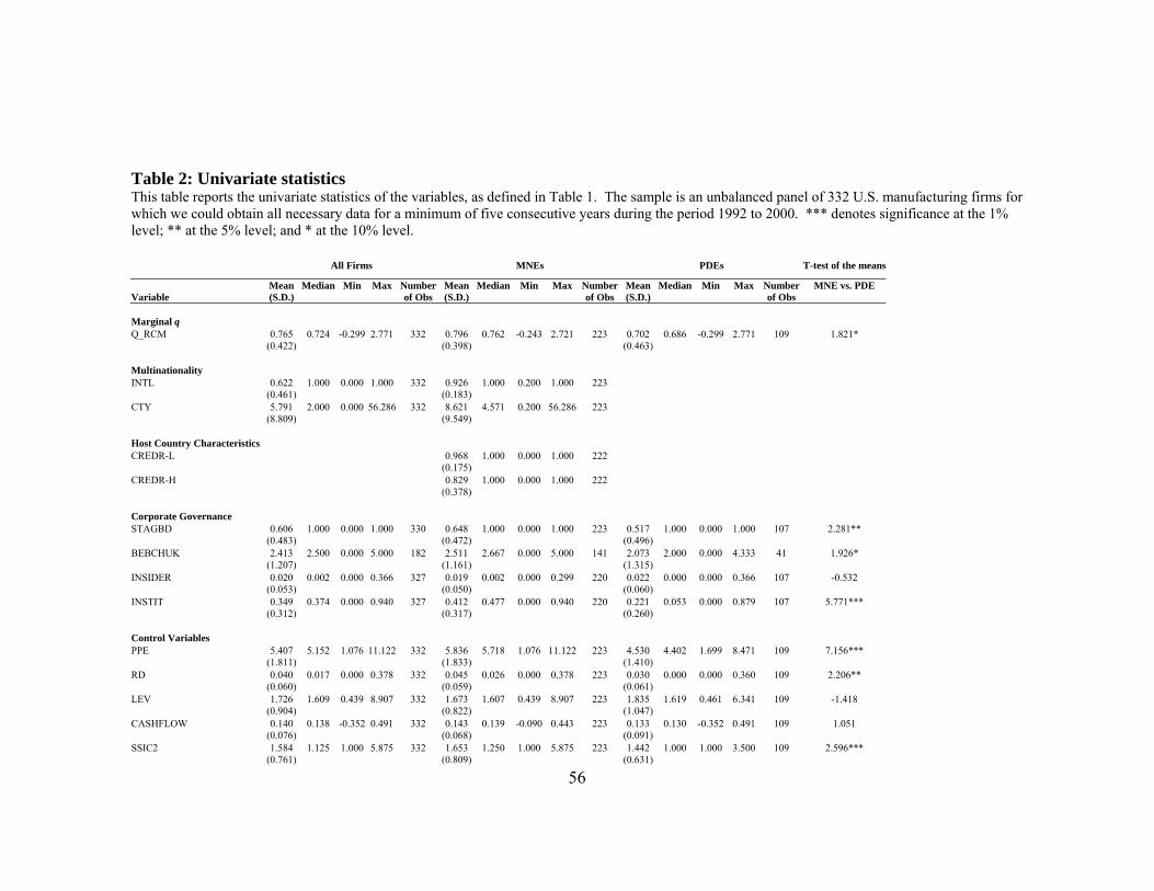
56
Table 2: Univariate statistics This table reports the univariate statistics of the variables, as defined in Table 1. The sample is an unbalanced panel of 332 U.S. manufacturing firms for which we could obtain all necessary data for a minimum of five consecutive years during the period 1992 to 2000. *** denotes significance at the 1% level; ** at the 5% level; and * at the 10% level.
All Firms MNEs PDEs T-test of the means
Variable Mean (S.D.)
Median Min Max Numberof Obs
Mean(S.D.)
Median Min Max Numberof Obs
Mean(S.D.)
Median Min Max Numberof Obs
MNE vs. PDE
Marginal q
Q_RCM 0.765 (0.422)
0.724 -0.299 2.771 332 0.796 (0.398)
0.762 -0.243 2.721 223 0.702 (0.463)
0.686 -0.299 2.771 109 1.821*
Multinationality
INTL 0.622 (0.461)
1.000 0.000 1.000 332 0.926 (0.183)
1.000 0.200 1.000 223
CTY 5.791 (8.809)
2.000 0.000 56.286 332 8.621 (9.549)
4.571 0.200 56.286 223
Host Country Characteristics
CREDR-L 0.968 (0.175)
1.000 0.000 1.000 222
CREDR-H 0.829 (0.378)
1.000 0.000 1.000 222
Corporate Governance
STAGBD 0.606 (0.483)
1.000 0.000 1.000 330 0.648 (0.472)
1.000 0.000 1.000 223 0.517 (0.496)
1.000 0.000 1.000 107 2.281**
BEBCHUK 2.413 (1.207)
2.500 0.000 5.000 182 2.511 (1.161)
2.667 0.000 5.000 141 2.073 (1.315)
2.000 0.000 4.333 41 1.926*
INSIDER 0.020 (0.053)
0.002 0.000 0.366 327 0.019 (0.050)
0.002 0.000 0.299 220 0.022 (0.060)
0.000 0.000 0.366 107 -0.532
INSTIT 0.349 (0.312)
0.374 0.000 0.940 327 0.412 (0.317)
0.477 0.000 0.940 220 0.221 (0.260)
0.053 0.000 0.879 107 5.771***
Control Variables
PPE 5.407 (1.811)
5.152 1.076 11.122 332 5.836 (1.833)
5.718 1.076 11.122 223 4.530 (1.410)
4.402 1.699 8.471 109 7.156***
RD 0.040 (0.060)
0.017 0.000 0.378 332 0.045 (0.059)
0.026 0.000 0.378 223 0.030 (0.061)
0.000 0.000 0.360 109 2.206**
LEV 1.726 (0.904)
1.609 0.439 8.907 332 1.673 (0.822)
1.607 0.439 8.907 223 1.835 (1.047)
1.619 0.461 6.341 109 -1.418
CASHFLOW 0.140 (0.076)
0.138 -0.352 0.491 332 0.143 (0.068)
0.139 -0.090 0.443 223 0.133 (0.091)
0.130 -0.352 0.491 109 1.051
SSIC2 1.584 (0.761)
1.125 1.000 5.875 332 1.653 (0.809)
1.250 1.000 5.875 223 1.442 (0.631)
1.000 1.000 3.500 109 2.596***
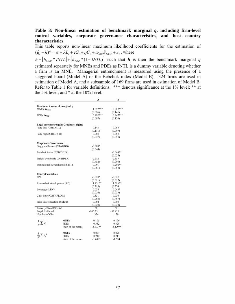
Table 3: Non-linear estimation of benchmark marginal q, including firm-level control variables, corporate governance characteristics, and host country characteristics
This table reports non-linear maximum likelihood coefficients for the estimation of , where iiSICSICiiii SCGLhq εωητλα +++++=− ,
2)ˆ([ ] [ )1(** INTLhINTLhh PDEMNE −+= ] such that h is then the benchmark marginal q
estimated separately for MNEs and PDEs as INTL is a dummy variable denoting whether a firm is an MNE. Managerial entrenchment is measured using the presence of a staggered board (Model A) or the Bebchuk index (Model B). 324 firms are used in estimation of Model A, and a subsample of 169 firms are used in estimation of Model B. Refer to Table 1 for variable definitions. *** denotes significance at the 1% level; ** at the 5% level; and * at the 10% level.
A B Benchmark value of marginal q MNEs: h 1.022*** 0.887*** MNE
(0.096) (0.141) PDEs: h 0.892*** 0.947*** PDE
(0.097) (0.120) Legal system strength: Creditors’ rights - any low (CREDR-L) 0.143 0.065
(0.111) (0.099) - any high (CREDR-H) 0.003 -0.082
(0.047) (0.058) Corporate Governance Staggered boards (STAGBD) -0.083*
(0.044) Bebchuk index (BEBCHUK) -0.064**
(0.025) Insider ownership (INSIDER) -0.212 -0.355
(0.452) (0.708) Institutional ownership (INSTIT) 0.091 0.202**
(0.061) (0.080) Control Variables PPE -0.020* -0.027
(0.011) (0.017) Research & development (RD) 1.731** 1.596**
(0.718) (0.774 Leverage (LEV) 0.038 0.068*
(0.026) (0.039) Cash flow (CASHFLOW) 0.331 0.030
(0.288) (0.467) Prior diversification (SSIC2) 0.004 0.000
(0.023) (0.024) Industry Fixed Effects? No No Log-Likelihood -105.35 -53.935 Number of Obs. 324 179
MNEs 0.195 0.196 ∑
iiN
ε1PDEs 0.332 0.328 t-test of the means -2.393** -2.429**
MNEs 0.077 0.076
∑i
iN2ˆ1 ε PDEs 0.212 0.213
t-test of the means -1.639* -1.554
57
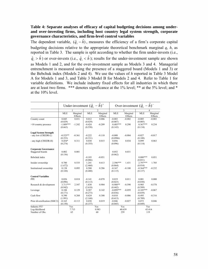
Table 4: Separate analyses of efficacy of capital budgeting decisions among under- and over-investing firms, including host country legal system strength, corporate governance characteristics, and firm-level control variables The dependent variable, , measures the efficiency of a firm’s corporate capital budgeting decisions relative to the appropriate theoretical benchmark marginal q, h, as reported in Table 3. The sample is split according to whether the firm under-invests (i.e.,
) or over-invests (i.e., ); results for the under-investment sample are shown as Models 1 and 2, and for the over-investment sample as Models 3 and 4. Managerial entrenchment is measured using the presence of a staggered board (Models 1 and 3) or the Bebchuk index (Models 2 and 4). We use the values of h reported in Table 3 Model A for Models 1 and 3, and Table 3 Model B for Models 2 and 4. Refer to Table 1 for variable definitions. We include industry fixed effects for all industries in which there are at least two firms. *** denotes significance at the 1% level; ** at the 5% level; and * at the 10% level.
)ˆˆ( hqi −
hqiˆˆ > hqi
ˆˆ <
Under-investment +− )ˆˆ( hqi Over-investment
−− )ˆˆ( hqi 1 2 3 4 MLE Marginal MLE Marginal MLE Marginal MLE Marginal
Effects Effects Effects Effects Country count 0.045 0.031 0.012 0.006 -0.003 -0.002 -0.005
(0.005) -0.003
(0.029) (0.029) (0.007) >10 country presence -1.809***
(0.663) -1.242 -0.424 -0.209 0.485***
(0.143) 0.290 0.367***
(0.134) 0.234
(0.558) Legal System Strength - any low (CREDR-L) -0.525** -0.361 -0.222 -0.110 -0.008 -0.004 -0.027 -0.017
(0.253) (0.331) (0.0986) (0.108) - any high (CREDR-H) 0.454* 0.311 0.030 0.015 0.056 0.034 0.099 0.063
(0.274) (0.355) (0.096) (0.114) Corporate Governance Staggered boards 0.002 0.001 0.052 0.031
(0.156) (0.062) Bebchuk index -0.103
(0.086) -0.051 0.080***
(0.031) 0.051
Insider ownership 0.780 0.535 1.241 0.613 2.396***(0.864)
1.431 2.797*** 1.785 (1.672) (2.460) (0.934)
Institutional ownership 0.138 0.095 0.580 (0.480)
0.286 -0.167 -0.100 -0.364*** -0.232 (0.320) (0.115) (0.137)
Control Variables PPE 0.026 0.018 -0.141 -0.070 0.019 0.011 0.001 0.000
(0.096) (0.113) (0.023) (0.030) Research & development 3.711*** 2.547 1.830 0.904 -0.988** -0.590 -0.905 -0.578
(0.942) (2.618) (0.442) (0.589) Leverage 0.188 0.129 0.287 0.142 -0.099*** -0.059 -0.105*** -0.067
(0.171) (0.273) (0.036) (0.039) Cash flow 0.390 0.268 0.624 0.308 -0.010 -0.006 -0.495 -0.316
(1.991) (2.168) (0.413) (0.709) Prior diversification (SSIC2) -0.165 -0.113 0.038 0.019 -0.046 -0.027 0.072 0.046
(0.150) (0.157) (0.045) (0.049) Industry FE? Yes Yes Yes Yes Log-likelihood 7.715 0.983 40.639 43.414 Number of Obs. 65 60 259 119
58