MULTINATIONALS AND US PRODUCTIVITY

LEADERSHIP: EVIDENCE FROM GREAT

BRITAIN ∗†

Chiara Criscuolo‡ Ralf Martin§

September 16, 2007

Abstract

We study the productivity of US and other foreign owned plants in the UK.Using a new dataset that can identify for the first time domestic UK MNEsin such a study, we find that UK MNEs are less productive than US affiliates,but as productive as non US foreign affiliates. Exploiting dynamic variationin our data, we find evidence suggesting that this additional US advantageis due to the takeover of already highly productive UK plants rather thanthe sharing of superior firm specific assets. The study also features a novelapproach to TFP calculation.

JEL Classification: F230, L600 Keywords: Multinational Firms, Pro-ductivity, Foreign Ownership, US leadership

∗This work contains statistical data from the Office of National Statistics (ONS) which is Crowncopyright and reproduced with the permission of the controller of HMSO and Queen’s Printer forScotland. The use of the ONS statistical data in this work does not imply endorsement of the ONSin relation to the interpretation or analysis of the statistical data.

†We thank two anonymous referees for extremely helpful comments, plus Lee Branstetter, TonyClayton, Richard Disney, Jonathan Haskel, Wolfgang Keller, John Haltiwanger, Steve Nickell, NickOulton, Steve Redding, Fergal Shortall, Alessandra Tucci, John Van Reenen, Prabhat Vaze andparticipants at the 2004 NBER Summer Institute. This research was conducted under contractwith the ONS. We gratefully acknowledge financial support from the Evidence-Based Policy Fundand from the ESRC/EPSRC Advanced Institute of Management Research, grant number RES-331-25-0030. Chiara Criscuolo thanks the ESRC, grant number PTA-026-27-0445, and the BritishAcademy for funding. Errors and opinions are those of the authors alone.

‡Centre for Economic Performance (CEP) London School of Economics (LSE), Centre forResearch into Business Activity (CeRiBA) and Advanced Institute of Management (AIM);c.criscuolo@lse.ac.uk

§Centre for Economic Performance (CEP), London School of Economics (LSE), Centre forResearch into Business Activity (CeRiBA), and Advanced Institute of Management (AIM);r.martin@lse.ac.uk

1

1 Introduction

International comparisons show that the US is the world’s most productive economy1

and much research has gone into understanding the determinants of this productiv-

ity leadership.2 Responsible for this success could be the business environment in

which US firms operate and/or technological factors (e.g. superior technologies for

designing products and production processes and better management) specific to

US firms. While the latter might themselves be determined by the business envi-

ronment,3 the distinction between business environment and technological factors is

interesting because of its implications for economic policy. A technological expla-

nation for the US lead, for example, could motivate policies to source this superior

technological knowledge from abroad.4 We examine these issues by looking at a

firm level dataset that automatically rules out environmental factors since all firms

in the sample are located in the same environment. Using data from the UK Of-

fice of National Statistics (ONS) that comprehensively covers the whole of the UK

manufacturing we compare the productivity performance of US multinationals in

Britain with those of other multinational enterprises (MNE) and domestic firms. A

number of existing studies have made similar comparisons for the UK.5 These stud-

ies have found that on average US firms in Britain are significantly more productive

than their domestic counterparts, which seems consistent with the explanation of

US productivity leadership being based on ‘technological factors’. However, care

should be taken in drawing such a conclusion from this evidence, for the following

reasons.

1see for example O’Mahony and de Boer (2002).2see for example Wagner and van Ark (1996), O’Mahony and van Ark (2003) or for a very

accessible discussion Lewis (2004).3e.g. the quality of the educational system might determine not only the skill level of a country’s

workforce but also its output of new technologies and its firms’ access to and adoption of thesetechnologies; institutional differences that affect market structure likely influence entrepreneurs’incentives to develop and adopt new technologies.

4An example of such a policy in the UK is the subsidies offered to US and other foreign multi-nationals to locate in Britain.

5see Griffith and Simpson (2001), Oulton (2000), Harris (1999).

2

Firstly, by definition, all foreign owned establishments in any country, and thus

all US owned establishments in Britain, must be part of a MNE. As has been sug-

gested by Dunning (1981), Helpman (1984), Markusen (1995) and more recently by

Helpman et al. (2004), MNEs can be expected to be at the upper end of the pro-

ductivity distribution in any country because factors such as language barriers and

ignorance of local business networks leave foreign firms at a disadvantage. If never-

theless MNE firms manage to stay in business, they must have superior firm specific

assets – such as better management techniques and better production technology –

which can be shared with their foreign affiliates and which give them an edge over

local competitors. In fact, even in the US, foreign owned firms are found on average

to be more productive than their domestic counterparts (Doms and Jensen, 1998).

To account for these aspects we therefore need to compare foreign owned firms with

domestic MNEs, and not to all domestic firms. Doms and Jensen (1998) did this in

the case of the US and found that foreign MNEs are less productive than US MNEs

in the US. This type of comparison for the UK has not been possible up to now as

the available data for the UK only included indicators for foreign ownership, but

not the multinational status of domestic firms.

Secondly, while Doms and Jensen (1998) results are consistent with a US tech-

nology lead this does not rule out the possibility that the US success is driven by a

home advantage: US MNEs enjoy a productivity advantage only in the US, where

they have a more intimate knowledge of local practices.

Finally, a major form of MNE entry into foreign markets is via takeovers of

existing plants. This is likely not a random process. If US MNEs systematically

take over firms that were already more productive then a US advantage in the UK

could emerge even without any transfer of superior knowledge or technology from

the US parent to its plant in the UK.

Our paper provides new results and progresses a number of issues. For the first

time we are able to identify domestic MNEs in the productivity dataset used in

3

earlier UK studies by combining it with data from the UK Annual Survey into

Foreign Direct Investment (AFDI). This shows that UK MNEs are significantly

more productive than domestic non-MNE firms. Using a wide range of different

productivity measures and robustness checks we find, like Doms and Jensen, that

US MNEs are on average more productive than all other MNEs. This suggests that

their finding was not driven by a home market effect.

Also we have annual plant level panel data for 1996 to 2000. Using the longi-

tudinal variation and changes in ownership of plants we examine whether this US

advantage is driven by plant picking effects rather than by knowledge or technology

transfer from the parent firm. The results suggest that this is indeed the case. While

we find a strong effect on productivity after takeover by an MNE,6 these effects are

not any stronger for takeovers by US MNEs, we find – using two different identifi-

cation strategies – that US MNEs tend to take over plants that are already more

productive prior to acquisition.

Finally, our dataset allows us to examine the technology sourcing hypothesis

(Branstetter, 2001; Keller, 2004). According to this hypothesis FDI might not be

driven by superior firms exploiting their advantage abroad (Dunning, 1981), but

rather by domestic firms trying to gain access to superior foreign technology. We

can examine this by looking at the productivity performance of domestic firms that

started to invest abroad during the sample period. – i.e. that became multinational

in 1996-2000. Although we did not find significant evidence for such an effect, this

might be due to the short panel available.

Our paper also makes a number of methodological contributions. Firstly, among

the productivity measures we employ to examine the robustness of our results we use

a new TFP (total factor productivity) estimator, derived from a structural produc-

tion function estimation approach; i.e. the estimator is similar to those proposed by

Olley and Pakes (1996) (OP) and Levinsohn and Petrin (2003) (LP) but addresses

6We refer to these as firm effects.

4

a number of shortcomings of these estimators.7

Secondly, we propose two new frameworks that separately identify firm and plant

effects. Both exploit the facts that we have plant level data, we know which plants

are under common firm ownership and we have sufficient switches of ownership of

plants between different firms. Our first framework posits a double fixed effects

model where the plant effect is the time invariant component of a plant’s produc-

tivity as it switches between firms and the firm effect is the time invariant compo-

nent as a firm owns different plants. Our second framework extends the structural

productivity estimator we use for our robustness checks by explicitly including a

multinomial selection model, which is simultaneously estimated with the produc-

tion function equation. This framework allows flexible mapping of the relationship

between pre-takeover performance and takeover. For example, we can easily exam-

ine whether an important determinant of takeover is the pre-takeover plant’s short

term rather than long-term performance.

The rest of the paper is organised as follows. In Section 2 we describe the

dataset. Section 3 outlines the econometric framework and the details of the two-

step estimation procedure used to disentangle the US productivity effect. Section 4

reports the results and Section 5 concludes.

2 The Data

2.1 Data Sources

Our sample is drawn from the Annual Respondents Database (ARD)8, which is the

UK equivalent of the US Longitudinal Respondents Database (LRD). The dataset

was made available by the ONS and is based on information from the Annual Busi-

7STATA code to implement the estimator can be downloaded fromhttp://193.93.28.107/pubtwik/bin/view/MP/TrueMethod.

8More extensive descriptions of the ARD can be found in Criscuolo, Haskel and Martin (2003),Griffith (1999) and Oulton (1997).

5

ness Inquiry (ABI), a mandatory annual survey of UK businesses.9 The ARD unit

of observation is defined by the ONS as an ‘autonomous business unit’. We refer to

this level of observation as a ‘plant’.10 It is important to note that the ARD does

not comprise the complete population of UK businesses. For example, businesses

located in Northern Ireland are excluded; all other businesses with more than 100

employees11 are surveyed, with smaller businesses being sampled randomly. Each

year the sampled plants account for around 90% of total UK manufacturing employ-

ment.12 The resulting sample is an unbalanced panel of about 19,000 manufacturing

plants which we observe annually for the years 1996 to 2000.

The country of ownership of a foreign firm operating in the UK – and thus the

ability to identify foreign owned MNE plants in the UK – is provided in the ARD.13

While this identifies foreign owned plants, it has not previously been possible to

identify UK MNEs. To do this we use the AFDI register.

The AFDI is an annual survey of businesses which requests a detailed breakdown

of the financial flows between UK firms and their overseas parents or subsidiaries; it

operates at firm rather than plant level. The ONS maintains a register that provides

the sampling frame for the AFDI and which holds information on the population

of all UK firms that engage in or receive FDI, on the country of ownership of each

foreign firm, and on which UK firms have foreign subsidiaries or branches and where

these are located.14 This register is designed to capture the universe of firms that are

9Annual Census of Production until 1998.10Some of these business units are spread across several sites and are therefore not plants in the

strictest definition. About 80% of the business units are located at a single mailing address.11In some years the threshold was 250 employees, for details refer to Criscuolo, Haskel and

Martin (2003).12To examine whether our results are sensitive to the oversampling of larger plants we ran

regressions with inverse sampling probabilities as weights. These results, available upon requestfrom the authors, are not qualitatively different from the unweighted results reported in the Resultssection.

13The ARD data are supplemented here with information from the Dun&Bradstreet global “WhoOwns Whom” database. According to Dun&Bradstreet, the nationality of a plant is determinedby the country of residence of the global ultimate parent, i.e. the topmost company of a Worldwidehierarchical relationship identified bottom-to-top using any company which owns more than 50%of the control (voting stock, ownership shares) of another business entity.

14The working definition of FDI for this purpose is that the investment must give the investing

6

involved in FDI abroad and in the UK. We consequently define as ‘multinational’

each plant in the ARD that is owned by a firm that appears in the AFDI register.15

One problem with the AFDI register is that information is not always up to

date. If a firm engages in or receives FDI, it will only be included in the AFDI

register after the ONS learns about this from external sources, including commercial

data and newspapers. Consequently, the register population has varied, somewhat

spuriously, over the years with the ONS’s success in identifying such firms. However,

we believe that this problem does not weaken the conclusions that can be drawn

from our results. If some of the plants recorded as non-multinational were actually

part of a MNE, the estimated productivity gap would be a lower bound of that

found using data free from measurement errors.

2.2 Descriptive Evidence

Table 1 shows the number of multinational plants that we can identify in the pop-

ulation and in the sample and their relevance in terms of employment and value

added.

Column 1 reports the number of domestic plants with no FDI, (defined as UK

non MNEs), British MNEs (UK MNE), US MNEs (US) and Non-US foreign owned

plants (FOR) in the whole population. Column 2 shows the number of plants in

each group for the sample surveyed by the ONS to compile the ARD. Columns 3

and 4 translate these numbers into shares. Column 3 shows that 1% of all plants in

Britain are US owned, as big a percentage almost as all other foreign owned plants

firm a ‘significant’ level of control over the recipient firm. The ONS considers this to be thecase if the investment gives the investor a share of at least 10% of the recipient firm’s capital.The ONS further distinguishes between subsidiaries and branches as follows: a ‘subsidiary’ is acompany where the parent company holds more than 50% of the equity share capital; a ‘branch’ isa permanent establishment as defined for UK corporation tax and double taxation relief purposes;companies where the investing company holds between 10% and 50% of the equity share capital,i.e. does not have a controlling interest, but participates in the management, are defined as‘associates’. The country of ownership is identified by the nationality of the immediate owner,Office for National Statistics (2002) p.120.

15Details of the procedure followed to merge the AFDI and the ARD are reported in Criscuoloand Martin (2003).

7

Table 1: Importance of MNE(Average numbers and shares 1996-2000)

number of plants shares employment share value added share(1) (2) (3) (4) (5) (6) (7) (8)pop. sample pop. sample pop. sample weighted unweighted

UK Non MNE 158,868 8,394 0.96 0.75 0.59 0.41 0.44 0.31UK MNE 3,062 1,427 0.02 0.13 0.21 0.29 0.27 0.32US 1,172 615 0.01 0.05 0.10 0.14 0.15 0.19FOR 1,708 825 0.01 0.07 0.11 0.16 0.14 0.18

Notes: Figures reported are annual averages. Population refers to all businesses in the register, sample refers tobusinesses in the ARD (all large plants plus a stratified sample of smaller plants). Column 5 uses employmentinformation from administrative data for non-surveyed plants. Columns 7 and 8 use value added at factor cost.Column 7 weights surveyed observations using employment weights calculated as described in the Appendix A toyield statistics representative of the whole population. UK non MNE denotes domestic plants with no FDI; UKMNE denotes all domestic multinationals; US all plants owned by a US multinational and FORall plants owned by non-US foreign multinationals.Source: Authors’ calculations using matched ARD-AFDI data for the period 1996-2000.

combined. Indeed, US MNEs represent more than 40% of all foreign owned plants in

Britain ((615+825)/825). Figures are similar for shares in employment (Column 5)

and value added (Column 7), where US owned plants represent 47 and 51% of FDI,

respectively. These figures are consistent with the fact that the most productive

companies are also likely to have the highest market share. Also, since US MNEs

are on average larger, the relative share of US MNEs in the selected sample is much

higher: whereas in the total population US MNEs take a share of about 1%, in the

sample the same figure rises to 5%.

Table 2 reports averages and standard deviations for relevant variables. Panel

1 shows the US owned plants’ labour productivity lead: averaging over the whole

manufacturing sector and not controlling for industry we find that plants owned by

US firms have an advantage of 26% ((46.57− 36.87)/36.87) over British MNEs and

an advantage of 8% ((46.57 − 43.10)/43.10) over other foreign MNEs. In terms of

gross output per employee (panel 2) the ranking changes: foreign non-US owned

plants are the most productive and, in general, the foreign advantage becomes more

dramatic. Panels 3 and 4 suggest that the figures in panel 2 can be explained in

part by the fact that non-US foreign owned plants have much higher materials-to-

labour and capital-to-labour ratios than all other plants. Panel 5 shows that US

8

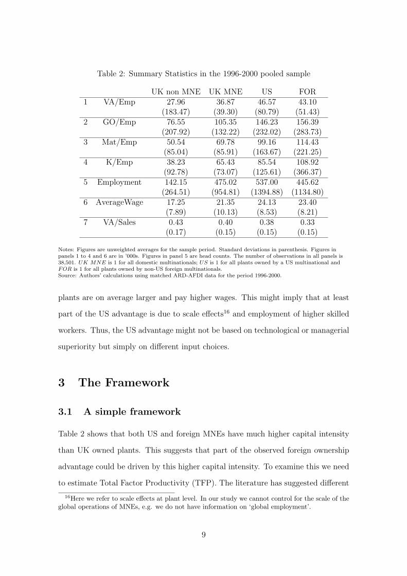
Table 2: Summary Statistics in the 1996-2000 pooled sample

UK non MNE UK MNE US FOR1 VA/Emp 27.96 36.87 46.57 43.10

(183.47) (39.30) (80.79) (51.43)2 GO/Emp 76.55 105.35 146.23 156.39

(207.92) (132.22) (232.02) (283.73)3 Mat/Emp 50.54 69.78 99.16 114.43

(85.04) (85.91) (163.67) (221.25)4 K/Emp 38.23 65.43 85.54 108.92

(92.78) (73.07) (125.61) (366.37)5 Employment 142.15 475.02 537.00 445.62

(264.51) (954.81) (1394.88) (1134.80)6 AverageWage 17.25 21.35 24.13 23.40

(7.89) (10.13) (8.53) (8.21)7 VA/Sales 0.43 0.40 0.38 0.33

(0.17) (0.15) (0.15) (0.15)

Notes: Figures are unweighted averages for the sample period. Standard deviations in parenthesis. Figures inpanels 1 to 4 and 6 are in ’000s. Figures in panel 5 are head counts. The number of observations in all panels is38,501. UK MNE is 1 for all domestic multinationals; US is 1 for all plants owned by a US multinational andFOR is 1 for all plants owned by non-US foreign multinationals.Source: Authors’ calculations using matched ARD-AFDI data for the period 1996-2000.

plants are on average larger and pay higher wages. This might imply that at least

part of the US advantage is due to scale effects16 and employment of higher skilled

workers. Thus, the US advantage might not be based on technological or managerial

superiority but simply on different input choices.

3 The Framework

3.1 A simple framework

Table 2 shows that both US and foreign MNEs have much higher capital intensity

than UK owned plants. This suggests that part of the observed foreign ownership

advantage could be driven by this higher capital intensity. To examine this we need

to estimate Total Factor Productivity (TFP). The literature has suggested different

16Here we refer to scale effects at plant level. In our study we cannot control for the scale of theglobal operations of MNEs, e.g. we do not have information on ‘global employment’.

9

approaches for estimating plant level TFP.

The most common approach is to assume that firms produce according to a

Cobb-Douglas production technology:

qit = γ∑z∈Z

αzxzit + ait (1)

where qit is the logarithm of output produced at plant i in period t, γ is the returns

to scale coefficient, Z is a set of production factors – labour (L), physical capital (K)

and intermediate inputs (M), all expressed in logs – αz are the production function

parameters, and ait is TFP.

With the data available we can start by examining whether TFP varies sys-

tematically between multinationally owned and domestic plants by running an OLS

estimation of the following equation

rit − pIt − xLit = γ(αM(xMit − xLit) + αK(xKit − xLit)) + (γ − 1)xLit

+β1USJ(i,t) + β2FORJ(i,t) + β3MNEJ(i,t)

+θIt + ψR + εit

(2)

i.e. we regress deflated revenue, rit − pIt,17 per worker, xLit, on inputs, ownership

dummies18 interacted dummies, θIt, to control for 4-digit sectors time effects and 10

regional dummies ψR to control for location effects within Britain.19

This approach – although standard practice – raises a number of concerns.

Firstly, OLS will be inconsistent if the plant’s factor input choices are determined

17At plant level we observe nominal sales rit = qit + pit but since we do not have plant levelinformation on prices, we deflated nominal sales using (four-digit) sector level price deflators pIt

18USJ(i,t), for example, would be equal to 1 if plant i is owned in period t by US firm J.19In our results section we further break down the other foreign and MNE categories to account

for possible heterogeneity within those groups. In particular, we distinguish between ‘EU-owned’multinationals and ‘non-EU-owned’ multinationals because EU MNEs are more likely to operateunder the same regulatory environment and to make sure that the US effect does not merely reflecta ‘non-EU’ effect. We then want to isolate UK multinationals that are as comparable as possibleto US affiliates. One way of doing this is to separate out from the UK multinationals group thoseUK MNEs that invest in the US.

10

by TFP as is likely to be the case. Secondly, since we only observe sectoral, not

plant level prices, deflated revenue, which forms the LHS variable in equation 2

corresponds to output quantities Q in equation 1 only under perfect competition.

Thirdly, the assumption of a Cobb-Douglas production function is very restrictive.

Our main tool to account for these issues is a modified version of the framework

suggested by Olley and Pakes (1996), which is new to the literature.

3.2 A more flexible approach

To overcome the limitations outlined above using the data we have we start with an

approach originally introduced by Klette and Griliches (1996) and Klette (1999) to

integrate a more flexible production function into a setting of imperfect competition.

We assume that firms produce according to a homogenous o degree γ general

differentiable function f(·):Qit = Ait [f (Xit)]

γ (3)

where Xit is a vector of factor inputs.

Also, using the data available, we can only observe nominal revenues – quantity

times price in logs qit + pit – deflated using (four-digit) sector level price deflators

pIt since plant level prices are not observed; i.e.

rit − pIt = qit + pit − pIt (4)

To control for unobserved plant level prices we specify a demand function that

links prices to output as follows (see also Melitz (2000)):

Qit =

(Pit

PIt

)−η

Λη−1it ΘIt (5)

where subscripts i denote firm and I industry; Λit is a firm specific demand shock,

11

η is industry demand elasticity and ΘIt is a sectoral shock to demand.20 Taking the

logs of Equation 5 and inverting gives:

pit − pIt =1

µλit − 1

ηqit +

1

ηθIt (6)

where µ = 11− 1

η

is the mark-up of price over marginal cost implied by profit maxi-

mizing behaviour and lower case letters denote logarithms.

Combining equations 6 and 1 with 4 gives:21

rit − pIt =γ

µ

∑z∈Z

αzxzit + ωit +1

ηθIt (7)

where ωit = 1µ

(ait + λit).

Klette showed that using the mean value theorem we can write the production

function relative to the median firm as:

qit = ait +∑z∈Z

αzxzit (8)

where small letters with a tilde denote log deviations from the median plant (M) in

a given year,22 and αz represent the partial derivative of the log production function

evaluated at some point Xit in the convex hull spanned by Xit and XMt, so that

αz = γfz(Xit)Xzit

f(Xit)(9)

where fz(·) represents the partial derivative of f(·) with respect to production factor

z.

20This demand function can be derived by assuming monopolistic competition a la Dixit-Stiglitz(see Dixit and Stiglitz, 1977) in the product market.

21As stressed by Klette and Griliches (1996) – the interpretation of the estimated coefficientson the production factors is different from that in equation 1 as they are now all divided by themark-up coefficient µ.

22e.g. qit = lnQit − lnQMt

12

The first order condition of profit maximization implies that

PitγQit

f(Xit)fz(Xit) = µWzit (10)

i.e. prices are such that the marginal value product is the mark-up µ times the

marginal cost W of each factor.

As pointed out by Klette (1999), equation 10 can only be expected to hold for

production factors that are easily adjustable. We assume that this is the case for

intermediates and labour, but not for capital, thus:

αz = µWzXzit

PitQit

= µszit (11)

where szit is the revenue share of factor z and z ∈ {L,M}. Further, because of the

homogeneity of degree γ of the production function we get

αK = γ − αL − αM (12)

and therefore in equation 8:

qit = ait + µviit + γkit (13)

where

viit =∑

z 6=K

sjt(xzit − kit) (14)

is an index of all variable factors. These results allow us to rewrite 7 as23

rit − viit =γ

µkit + ωit (15)

23All aggregate expressions such as pIt and θIt in 7 disappear because the equation is now writtenin terms of deviations from the median plant in the sector.

13

The variable factor index viit can be directly observed from the data, since it only

requires information on factor inputs and their revenue shares.24

Equation 15 suggests that the final element required to derive an estimate for ωit

is an estimate of βK = γµ, the ratio between the scale and the mark-up coefficients.

But plant level capital stocks – like all other inputs – are presumably highly corre-

lated with ωit,25 we address this problem using a modified version of the Olley and

Pakes (1996) (OP) approach and assume that ωit evolves as a first order Markov

Process:

ωit = E{ωit|ωit−1}+ νit (16)

We also assume that capital is only correlated with the expected component of

ωit but not with νit.26 Then we can estimate equation 15 if we find a control for

E{ωit|ωit−1}. In Appendix B we show that conditional on capital and assuming that

mark-ups µ are constant across firms in a narrowly defined sector (4-digit) there is

a monotone relationship between profits – defined as revenues minus variable costs

– and ω. Consequently we can invert the profit function and write

ωit = φω

(kit, Πit

)(17)

We do not know the functional form of E{ωit|·}, but we express it as a function of

observables in equation 17 so that we can rewrite 15 as

rit − viit =γ

µkit + g(kit−1, Πit−1) + νit (18)

24Equation 9 suggests that we should evaluate the derivatives – and thus the factor shares –at ‘some point in the convex hull’. Since we do not know the exact location of this point andof course we do not know the functional form of the derivative, we follow accepted practice andapproximate by averaging over the factor share at plant i and the factor share at the median plantM to calculate the shares in viit; i.e. sit = sMt+sit

2 . See also Baily et al. (1992) on this.25see Griliches and Mairesse (1995) for a summary of the endogeneity problem and potential

solutions.26Olley and Pakes assume that investment in t can only be used for production in t+1. We take

a different assumption, i.e. that investment is predetermined. Although this would be problematicin the Olley and Pakes methodology, it does not affect our estimation procedure.

14

where g(·) = E{ωit|φ(·)} is a function of unknown form. To estimate equation 18

we can either employ a semi-parametric procedure or approximate g(·) by a third

order polynomial. For simplicity, we adopt the latter strategy. An estimator for ωit

can then be derived as

ˆωit = rit − viit −(

γ

µ

)kit (19)

Concerning the method used to correct for endogeneity of factor inputs we would

like to stress that compared to Olley and Pakes (1996) the main innovation in

our approach is to use profits and not investment as a predictor for ωit. This has

a number of advantages. Firstly, a major criticism of the OP framework is that

investment might be a very poor predictor of the fixed component of ωit.27 If firms

are essentially in a steady state – and the capital stock in period t reflects the firm’s

knowledge about ωit at t − 1 – then the variation in investment primarily reflects

adjustments to news about ω from period t. Our approach – similar to Levinsohn

and Petrin (2000) who use material inputs rather than investment – does not suffer

from this problem. Plants with high ω will have higher profits whether or not they

are in steady state. Secondly, and unlike Levinsohn and Petrin, we can identify all

relevant parameters from a moment condition on capital without having to assume

separability in intermediate inputs or to rely on instrumental variable techniques.

Also, we do not require any assumptions about substitutability between variable

production factors.28

Finally, to examine whether measured TFP (ωit) systematically differs between

various types of MNEs we run a regression of ωit from equation 19 on our ownership

dummies.

ˆωit = β1USJ(i,t) + β2FORJ(i,t) + β3MNEJ(i,t) + εit (20)

How do we interpret TFP, here denoted as ωit (and ˆωit)? Without plant level price

27see Griliches and Mairesse (1995).28For a more detailed discussion of our approach see Martin (2003).

15

information it is no longer possible to regard TFP as a shift parameter relating

solely to technical efficiency.29 Rather, ωit = 1µ

(ait + λit) is a composite of technol-

ogy shocks ait, demand shocks λit and mark-up µ. How does this affect the way

we interpret the MNE, US and FOR dummies in equation 20? If we assume that

within 4-digit sectors µ is constant, a higher ωit for US and MNE plants reflects

higher product quality and/or consumer valuation λit, and/or higher technical ef-

ficiency, ait. However, if µ is not constant within 4-digit sectors, then a higher ωit

might reflect greater market power, as recent papers30 have demonstrated. This

implies that revenue based measures of TFP (ωit) might vary between plants for

reasons other than product quality and technical efficiency. If within-sector differ-

ences in market power are positively related to the composite of technical efficiency

and product quality (ait +λit) then revenue based TFP provides a downward biased

estimate of ‘real’ TFP.31 Foster et al. (2003)32 find a positive relationship between

market power and product quality, (λit) here. If this is the case the MNE advantage

estimated under the assumption of constant mark-ups within sectors is a downward

biased estimate of the ‘true’ advantage that exists in the presence of within-sector

differences in mark-up.33

Since we do not have firm-level prices, in order to ensure that our results are not

driven by multinationals having greater market power than domestic firms we did

two checks.

First, we devised a test – based on over-identifying restrictions – of the assump-

29Melitz (2000) stresses this point.30see for example Foster, Haltiwanger and Syverson (2003), Syverson (2004) and Katayama, Lu

and Tybout (2003).31If in equation 7 the coefficients on factor inputs vary because of differences in market power

across plants (µit) but our estimation model uses fixed coefficients µt ∈ [min{µit};max{µit}] andCov(µit, ait+λit) > 0, then for plants with high (ait+λit) we attribute too much output variation toproduction factors. More intuitively, this is the case because our regression model does not controlfor the fact that for plants with larger µit an increase in factors would lower prices relatively more.

32One of the few productivity studies to use a dataset with firm level prices.33The reason for this result is that the assumption of constant mark-up leads to TFP estimates

for better plants, such as MNEs, which are downward biased.

16

tion that µ in equation 7 is constant.34 The hypothesis that µ is constant is rejected

in a large number of sectors. We estimated our preferred specification only on plants

in those sectors where we cannot reject the null of a constant µ. The estimates show

the same productivity ranking for MNEs as found in the whole sample.

Second, we tried to identify sectors where market power might be less likely

to drive the rankings. We assume that in commodity producing sectors35 the as-

sumption of constant mark-up within 4-digit industries is more likely to hold than

in non-commodity sectors where multinationals might have more market power, for

example because of stronger brands, and therefore might be able to command higher

prices.

An alternative, and possibly the simplest way to handle the endogeneity prob-

lem in production function estimations is to follow a factor share approach, which

involves no regression analysis at all but requires the assumptions of perfect com-

petition and constant returns to scale to hold.36 Following Baily et al. (1992) and

adopting a similar strategy to that used to calculate the variable factor index viit in

the previous subsection37 we calculate TFP as

ωBHCit = rit − sMitmit − sLitlit + (1− sMit − sLit)kit (21)

and check the robustness of our results to using this measure of TFP as left-handside

variable.

34The details of this test are reported in Appendix C35We identify these using Rauch (1999) classification.36An alternative method to estimate TFP controlling for the endogeneity of inputs would be

Difference GMM (Arellano and Bond (1991)) and System GMM (Blundell and Bond (1998)). Weapplied these estimation methods to our sample, but encountered two problems: first the timeperiod of our sample, 5 years, is too short, and less than 7% of the plants are observed over thewhole time period; secondly, due to the fact that the ARD surveys small plants randomly, there iscontinuous time series information for only 12% of the plants

37This approach is equivalent to imposing γµ = 1 which rules out imperfect competition and

non-constant returns to scale.

17

3.3 Explaining the sources of the US and MNE productivity

advantage

In this section we develop two different strategies to separately identify plant and

firm contributions to plant productivity. As discussed in the introduction, the higher

productivity of a plant owned by an MNE could be attributed to different factors.

Firstly, the parent firm might possess some superior knowledge and other trans-

ferable assets that improve the performance of its subsidiaries (best firm effect).38

Examples include international distribution networks, special management tech-

niques, patents, blueprints and reputation effects.

Secondly, MNE firms might be better at picking plants with superior performance

(plant picking effect); for example, multinational firms might be able to take over the

best plants because of deeper pockets to finance their takeover activities or higher

ability to spot top performing plants.

A third reason for higher MNE plant productivity is the going global effect:

plants owned by firms that start investing abroad might experience productivity

improvements as a direct consequence of FDI because of firm-level scale economies,

cheaper options to hedge against exchange rate risk, technology sourcing from abroad

or other learning effects.

3.3.1 A double fixed effect approach

We first distinguish between these various effects using a double fixed effects ap-

proach. Thus we write productivity of plant i at time t, ωit, as:39

ωit = αi + ζt,J(i,t) + εit (22)

38We can think of this effect as the ‘ownership specific’ factors in Dunning’s explanation of FDIor the ‘knowledge capital’ of the firm in Markusen (1995).

39For simplicity at this stage we do not separate the MNE group further into US and other foreign(FOR). We reintroduce these in the empirical analysis below. Also, in the empirical implementationwe use an estimate of ωit the residual from equation 2 as reported in Column 5 of table 3.

18

i.e. productivity can be decomposed into an effect ζt,J(i,t) due to the parent firm of

plant i at time t and a plant specific effect αi.40 The parent firm effect ζt,J(i,t) is then

decomposed further in a time invariant firm specific effect ζJ(i,t) and a time varying

effect that captures the productivity effects from becoming a multinational, βMNE;

i.e.

ζt,J(i,t) = ζJ(i,t) + βMNEMNEJ(i,t) (23)

so that

ωit = βMNEMNEJ(i,t) + αi + ζJ(i,t) + εit (24)

How do we identify and estimate the different determinants of the multinational

advantage in this setting? The best firm effect implies that MNE firms - both

foreign and British - have a higher firm specific fixed effect:

ζJ(i,t)∈MNEfirms > ζJ(i,t)/∈MNEfirms (25)

where MNEfirms is the set of firms in our sample that are multinational at some

point during our sample period. Similarly, to investigate the presence of a plant

picking effect we test that plant specific fixed effects are higher for plants that are

owned by MNEs; i.e.

αi∈MNEplants > αi/∈MNEplants (26)

where MNEplants is the set of plants that are owned by an MNE at some point

during the sample period. Finally, the going global effect, is represented as βMNE >

0.

To separately identify these different effects we use changes in ownership status

over the course of our sample period. For the identification of the going global effect

we look at UK domestic firms that start investing abroad - i.e. become MNEs -

during our sample period. For identifying the best firm and plant picking effects

40For simplicity of exposition we abstract from differences between types of MNEs.

19

we look at the performance of plants as they change ownership between MNE and

non MNE firms. Figure 2 in Appendix D illustrates the identification strategy using

an example. Table 7 in Appendix D presents evidence that reassures us that our

data have sufficient transitions of firms between multinational states, and of plants

between different types of firms.

The estimation of these effects proceeds in two steps. The first step is a pro-

ductivity regression where we control for every firm-plant combination fixed effect

so that in equation 24 this will cancel out both the firm and plant specific fixed

components, αi and ζJ(i,t).

˜ωit = ˜MNEJ(i,t)β + εit (27)

where a tilde represents the fixed effects within transformation.41 If endogenous

selection into the multinational group is entirely driven by the firm and plant spe-

cific fixed effects - an assumption we relax in our second approach below - then a

regression of equation 27 provides a consistent estimate of the causal productivity

impact of being an MNE; i.e. a positive going global effect would imply βMNE > 0.

With an unbiased estimate of βMNE we can estimate the firm-plant combination

fixed effects:

ζJ(i,t) + αi = ωit − βMNEMNEJ(i,t) (28)

This provides the basis for our second stage regression where we regress the predicted

fixed effects on two dummies variables MNEeverJ and MNEever

i . MNEeverJ is equal

to one for firms that are MNEs at any point during the sample. Similarly, MNEeveri

is equal to one for plants that are owned by MNEs in any year in the sample period.

41i.e. xit = xit − 1#it[J(i,t)]

∑τ s.t.J(i,τ)=J(i,t) xiτ where #it [·] is a function that returns the

number of periods plant i is owned by the firm J(i, t).

20

Formally, the second stage is

ζJ(i,t) + αi = βeverJ MNEever

J(i,t) + βeveri MNEever

i + υit (29)

The plant picking effect is βeveri > 0 and the best firm effect βever

J > 0.

What are the potential concerns in this analysis? A strong assumption in our

identification strategy is that all unobserved heterogeneity can be captured by our

two fixed effects. There might be important deviations from this assumption. In

particular we are concerned that takeover by a MNE is likely correlated with time

varying shocks, as well as plant fixed effects. For example, the transition to foreign

ownership might depend not only on a plant’s fixed characteristics, but also on its

time varying characteristics and idiosyncratic shocks. These might make plants more

likely to be taken over because they are temporarily weak and thus an easy target for

a hostile foreign takeover, or because MNEs become interested in a particular plant

only after a positive productivity shock, which might reveal better future growth

potential. In the next section we describe a possible estimation strategy that allows

us to correct for this source of endogeneity.

3.3.2 Correcting for endogeneity of becoming a multinational

In this section we develop an econometric framework that controls for endogeneity

in the probability of becoming part of an MNE42 incorporating the effects of MNE

ownership and takeover selection effects into the structural productivity estimation

framework described in Section 3.2.43 We incorporate takeover selection by explicitly

integrating a choice model as a step in the estimation. The plant picking effect is

then measured by the extent to which productivity prior to takeover influences the

42Of course, the ideal set-up to examine firm effects would be a randomized sample of planttakeovers by the different types of MNEs. Such data are not available.

43This implies that we control for endogeneity and plant level shocks can evolve as a generalMarkov Process.

21

occurrence of an MNE takeover.44

To describe our framework we start by only considering two ownership states

for notational simplicity: whether a plant is owned by an MNE or not.45 Also, we

follow the control function approach described in the previous section and assume

that ω can be decomposed as:

ωit = ωit + βMNEMNEJ(it) (30)

where ω evolves as follows: ωit = g(ωit−1)+νit. If MNE ownership is correlated with

ωit we have to include ownership status as an additional variable together with net

revenue and physical capital in the control function:

ωit = φω(πit, kit,MNEJ(it)) (31)

Secondly, if firms systematically select plants they take over this likely influences

expectations about plant level ωs. Hence, in the second stage of the OP-style pro-

cedure we get

Et−1{ωit} = g(ωit−1) + βEit−1{MNEJ(it)}+ νit (32)

or

Et−1{ωit} = g(ωit−1) + βPit−1 + νit (33)

where in the last equation we use the fact that Eit−1{MNEJ(it)} = Pit−1; i.e. that

the expectation at t − 1 of being an MNEat time t is the probability of becoming

an MNE in the next period.46

44For simplicity we start by looking at productivity in the year immediately prior to the takeover;we then extend the model to allow longer lags to influence the takeover choice.

45The framework immediately extends to the more general case of multiple ownership states,which we use in our actual implementation.

46If this probability is affected by ωit−1 then identifying the parameters of g(ωit−1) as opposedto those of βMNE and Eit−1{MNEJ(it)|Pit−1} might not be straightforward. However, since in

22

We then get an estimate of Pit−1 by running a discrete choice model of becoming

an MNE on a set of explanatory variables for each time t:

Pit = p(ρωωit + ρkkit + ρMNEMNEit) (34)

The MNE dummy captures that MNE ownership in the current period is likely

to increase the probability of MNE ownership in the next period.47 The takeover

decision is also likely influenced by other factors such as the size of the capital

stock – since larger plants with more valuable assets might, all else being equal, be

more interesting takeover candidates – and by longer lags of ωit.48 Of course ω is

not directly observable, but as before it can be controlled for by capital and net

revenue.

The estimation proceeds as follows: we first run a logit49 of the probability of

becoming part of an MNE (i.e. MNE takeover) on capital, net revenue and ownership

status:

Pit = p(φP (πit, kit,MNEit)) (35)

where φP (·) is a general function approximated by a polynomial. We then estimate

the following equation:

rit − viit = φ(kit, MNEJ(i,t), πit, Pit) + ηit (36)

stage 2 we only need to identify the capital coefficient of the production function we introduce acombined function; i.e. Et−1{ωit} = g(ωit−1, Pit−1) + νit

47We report results that take into account average plant performance before takeover as well ascurrent performance. For notational simplicity in this section we only include current performance.

48This could be particularly important if there are information asymmetries between plants andMNE firms and MNEs learn about plants by observing them over several periods.

49In our actual results we have different MNE states. Therefore we estimate a multinomial logitmodel. A more general approach would be to use a multinomial probit. However this would leadto computational intractabilities (Hajivassiliou and Ruud, 1993). While this can be addressed byemploying a simulation based inference approach this was beyond the scope of the current paper.

23

where φ(·) is again approximated by a polynomial to smooth out ηit. Note that

ωit = φ(kit,MNEJ(i,t), πit, Pit))− βkkit − βMNEJ(i,t) (37)

Using the assumption of a Markov process in ωit we can obtain an estimate for βk

and β from a non-linear least squares regression of

rit − viit = βkkit + βMNEJ(i,t)

+g(φ(kit−1,MNEJ(i,t−1), πit−1, Pit))− βkkit − βMNEJ(i,t)) + νit

(38)

which from 37 immediately gives us an estimator of ω. This allows us finally to

estimate equation 34:

Pit = p(ρωωit + ρkkit + ρMNEMNEit) (39)

In this setting the value of β gives us an estimate of the best firm effect and ρMNE

provides an estimate of the plant picking effect.50

4 Results

4.1 Evidence of the MNE and US productivity advantage

The labour productivity advantage of multinationals, US and non US, reported in

row 1 of Table 2 might reflect the fact that MNEs tend to operate in highly produc-

tive industries and/or tend to cluster in particular regions with special geographical

advantages. In fact, Figure 1 shows that MNEs are more present in medium to

50Since we have different types of MNEs: UK/other foreign and US, in practice we use a multi-nomial choice model allowing for 3 states: US MNE, other MNE (including UK), becoming UKMNE and to distinguish the going global (becoming UK MNE) from the MNE takeover effect - asin the fixed effects case – we include an ‘ever MNE’ as well as a current MNE dummy variable,both defined at firm level. Since the results of the double fixed effects approach show no indicationof strong going global effects we do not account for them in our second approach to avoid makingit too complex a framework.

24

high technology sectors such as chemicals and pharmaceuticals; paper; electrical

and optical equipment. Thus, we start our econometric analysis by controlling for

interacted 4-digit industry time fixed effects and regional dummies. The results of

this exercise are reported in Column 1 of Table 3, where we regress labour produc-

tivity, measured as real value added per employee on 4-digit industry year dummy

interactions, 10 regional dummies and two ownership dummies US, which equals 1

when a plant is a subsidiary of a US multinational, and FOR that takes the value

1 when a plant is owned by a foreign, non-US, corporation.

We find that US and other foreign owned plants are on average 42% and 30%

respectively more productive than British domestic plants.51 This sizeable advan-

tage is in line with previous results for Great Britain (e.g. Oulton, 2000). But how

much of this advantage is due to these plants being part of a multinational enter-

prise? Column 2 contains the answers to this question by including a multinational

dummy MNE that is 1 whenever a plant is owned by a multinational firm. If

this multinational is US owned the dummy US will be 1 as well. Consequently,

in Column 2 the US coefficient measures the advantage of US MNEs over British

MNEs and the FOR coefficient represents the advantage of Non-US foreign owned

subsidiaries over British MNEs.52 The coefficients’ estimates reported in Column 2

show that MNEs enjoy a productivity advantage of 30%, the US has a significant

additional advantage of 15%, while non-US foreign owned plants enjoy a smaller but

significant 5% advantage relative to their British counterparts.

Table 2 shows that both US and foreign MNEs have much higher capital intensity

than UK firms. This suggests that part of the observed foreign ownership advantage

could be driven by this higher capital intensity. To examine this we need to estimate

51The percentage differences reported in the text are calculated from the coefficients of thedummy variables in Table 3 according to the formula diff = (eβdummy − 1) e.g. for the US 0.42 =(e0.349 − 1).

52The performance of US MNEs relative to domestic plants can, therefore, be calculated as thesum of the coefficients on MNE and US and the advantage of other foreign-owned plants as thesum of the coefficients on MNE and FOR.

25

Figure 1: Share of MNE plants by 2 digit sectors

Notes: The sectors reported are at the 2-digit SIC92 level. 15 Food and beverages; 17 Textile; 18 Wearing apparel;19 Leather; 20 Wood and wood products; 21 Pulp, paper and paper products; 22 Publishing, printing andreproduction of recorded media; 24 Chemicals and chemical products; 25 Rubber and plastic products; 26 Othernon-metallic mineral products; 27 Basic metals; 28 Fabricated metals; 29 Machinery and equipment not elsewhereclassified (nec); 30 Office machinery and computers; 31 Electrical machinery and apparatus nec; 32 Radio,television and communication equipment and apparatus; 33 Medical, precision and optical instruments, watchesand clocks; 34 Motor vehicles, trailers and semi-trailers; 35 Other transport equipment; 36 Furniture,manufacturing nec; 37 Recycling. The figure reports shares of plants in each of the 2-digit sectors owned by UK;US and other foreign MNEs.

26

Tab

le3:

Rel

ativ

epro

duct

ivity

ofM

NE

(est

imat

esof

Equat

ion

2)(1

)(2

)(3

)(4

)(5

)(6

)(7

)(8

)

dep

.var

lnV

A Lln

GO L

US

0.3

49

0.1

44

0.0

76

0.0

45

0.0

44

0.0

33

0.0

72

(0.0

17)∗∗∗

(0.0

19)∗∗∗

(0.0

06)∗∗∗

(0.0

07)∗∗∗

(0.0

07)∗∗∗

(0.0

12)∗∗∗

(0.0

09)∗∗∗

FO

R0.2

61

0.0

55

0.0

41

0.0

10

0.0

09

0.0

37

(0.0

15)∗∗∗

(0.0

18)∗∗∗

(0.0

06)∗∗∗

(0.0

07)

(0.0

07)

(0.0

09)∗∗∗

MN

E0.2

61

0.0

47

0.0

47

0.0

47

0.0

47

0.0

20

(0.0

11)∗∗∗

(0.0

04)∗∗∗

(0.0

04)∗∗∗

(0.0

04)∗∗∗

(0.0

04)∗∗∗

(0.0

07)∗∗∗

EU

0.0

08

0.0

08

(0.0

07)

(0.0

07)

NO

N-E

U0.0

34

0.0

11

(0.0

07)∗∗∗

(0.0

11)

out

US

0.0

36

(0.0

08)∗∗∗

lnK L

0.0

71

0.0

70

0.0

72

0.0

72

0.0

72

0.0

72

(0.0

03)∗∗∗

(0.0

03)∗∗∗

(0.0

03)∗∗∗

(0.0

03)∗∗∗

(0.0

03)∗∗∗

(0.0

03)∗∗∗

lnM L

0.6

26

0.6

25

0.6

22

0.6

22

0.6

22

0.6

22

(0.0

05)∗∗∗

(0.0

05)∗∗∗

(0.0

05)∗∗∗

(0.0

05)∗∗∗

(0.0

05)∗∗∗

(0.0

05)∗∗∗

lnL

-0.0

10

-0.0

14

-0.0

10

-0.0

10

-0.0

10

-0.0

11

(0.0

02)∗∗∗

(0.0

02)∗∗∗

(0.0

02)∗∗∗

(0.0

02)∗∗∗

(0.0

02)∗∗∗

(0.0

02)∗∗∗

obs

38501

38501

38501

38501

38501

38501

38501

38501

Note

s:R

obust

standard

erro

rsin

pare

nth

eses

are

clust

ered

by

esta

blish

men

t,i.e.

robust

tohet

erosk

edast

icity

and

auto

corr

elati

on

ofunknow

nfo

rm.

InC

olu

mns

1and

2th

edep

enden

tvari

able

islo

gre

alvalu

eadded

(at

fact

or

cost

)per

emplo

yee

.In

Colu

mns

3to

8th

edep

enden

tvari

able

isth

epla

nt’

sre

algro

ssoutp

ut

per

emplo

yee

.B

oth

valu

eadded

and

gro

ssoutp

ut

are

defl

ate

dby

4-d

igit

annualoutp

ut

pri

cedefl

ato

rs.

Reg

ress

ions

inC

olu

mns

5to

8in

clude

aquadra

tic

poly

nom

ialin

age

and

an

age

censo

ring

dum

my

that

equals

1if

the

pla

nt

has

exis

ted

since

1980.

All

regre

ssio

ns

(Colu

mns

1to

8)

incl

ude

regio

nand

4-d

igit

indust

ryti

me

inte

ract

ion

dum

mie

s.U

Seq

uals

1if

apla

nt

isow

ned

by

aU

Sm

ult

inati

onal,

MN

Eis

1fo

rall

pla

nts

that

are

part

ofM

NE

firm

sand

FO

Ris

1fo

rall

pla

nts

ow

ned

by

non-U

Sfo

reig

nm

ult

inati

onals

.E

U(N

on−

EU

)des

crib

espla

nts

that

are

ow

ned

by

EU

(Non-E

U)

MN

Es;

OutU

Sis

1fo

rU

KM

NE

sth

at

have

affi

liate

sin

the

US.D

etails

ofth

eco

untr

ygro

up

class

ifica

tions

are

inth

eA

ppen

dix

A.∗

issi

gnifi

cantl

ydiff

eren

tfr

om

zero

at

the

10%

level

.∗∗

signifi

cantl

ydiff

eren

tfr

om

zero

at

the

5%

level

.∗∗∗

signifi

cantl

ydiff

eren

tfr

om

zero

at

the

1%

level

.

27

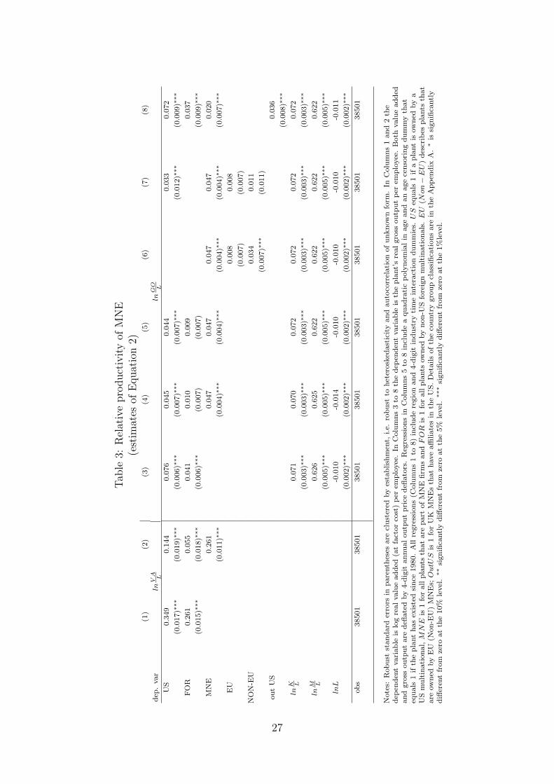
TFP. We start with the simple OLS approach summarized in equation 2.

In Column 3 – besides capital and material intensity and regional and industry

time effects – we only include US and non US foreign ownership dummies and

find that US owned plants are significantly the most productive plants in Britain

enjoying a strong and significant TFP advantage of almost 8% (with a coefficient

of 7.6 as shown by row 1 of Column 3) and non US foreign owned plants follow

with an advantage of 4% relative to the reference group of all British plants. This

confirms previous results (Griffith (1999), Oulton (2000) and Harris (1999)). Column

4 shows that once we include a separate dummy for being part of an MNE, the

advantage of non-US foreign MNEs drops to an insignificant 1%. US plants maintain

a significant advantage of 4.5% relative to British MNEs, which, in turn, are 4.8%

more productive than non-MNE plants. This result shows that only a part of the

US productivity advantage is actually a multinational effect. Column 5 accounts

for age effects by including a quadratic polynomial in age53 to account for possible

differences due to the plant life cycle, learning effects and/or the age of physical

assets. The coefficient on US MNE remains virtually unchanged, while the foreign

non-US advantage relative to UK MNEs is a non significant 1%. Finally, MNEs are

on average 4.6% more productive than British non-MNEs.

The aggregation of all non-US foreign owned plants in one group might hide

considerable heterogeneity. Therefore, in Column 6 of Table 3, we control for a

possible ‘EU’ effect and reclassify the MNE groups in EU (excluding UK MNEs) vs.

Non-EU MNEs.54 We find that that there is no statistically significant difference

between the UK and EU MNE coefficients while non-EU MNEs are significantly

more productive than EU MNEs. What is driving this difference? Column 7 shows

that once we separate US MNEs from non-EU MNE group, these are as before the

53Since our age variable is left censored in 1980, we include an age censoring dummy. Wehave tried alternative specifications for the age effect. We also experimented by including agecategories and the logarithm of age, which leads to the same conclusions obtained under thecurrent specification.

54details of the new country group classification can be found in Appendix A.

28

productivity leaders followed by all other MNEs. In Column 8 we report an addi-

tional robustness check for alternative definitions of multinationals. We distinguish

from the group of UK MNEs those that have affiliates in the US. The rationale

is that these multinationals are likely more similar to US MNEs;55 in fact when

checking the incidence of this group of UK MNEs we find that in our sample 77%

of UK MNEs have an affiliate in the US. The results show that US MNEs are still

the productivity leaders and that UK MNEs that have affiliates in the US are as

productive as other foreign MNEs and more productive than the 23% of UK MNEs

that do not have affiliates in the US.

Our results thus suggest the following. Firstly, controlling for capital intensity,

material usage, scale and age effects, US MNEs are the productivity leaders, with

British and non-US foreign MNEs having a comparable productivity advantage with

respect to British plants that are not part of an MNE. Secondly, much of the US and

all of the non-US foreign productivity advantage found in previous studies appears

to be an MNE effect.

4.2 Robustness checks

Several issues arise when estimating equation 2. Most of those we discussed already

in section 3.2: factor inputs might be endogenous and the production technology

might be more complex than Cobb-Douglas. Further, the regressions in Table 3

impose the same production technology for the whole manufacturing sector. Finally,

the assumption of perfect competition might not hold and the degree of market power

might vary between the different groups of MNE and non-MNE firms within 4-digit

sectors. We examine the robustness of our results to all of these concerns using a

number of different TFP estimation approaches, and also restricting the estimation

to different subsamples of our data. The results reported in Table 4 show that our

55Since both group of firms operate in the UK and the US. Ideally, one should compare MNEsthat invest in the same set of third countries. However, the data do not contain information onFDI destinations other than the UK, for foreign owned MNEs.

29

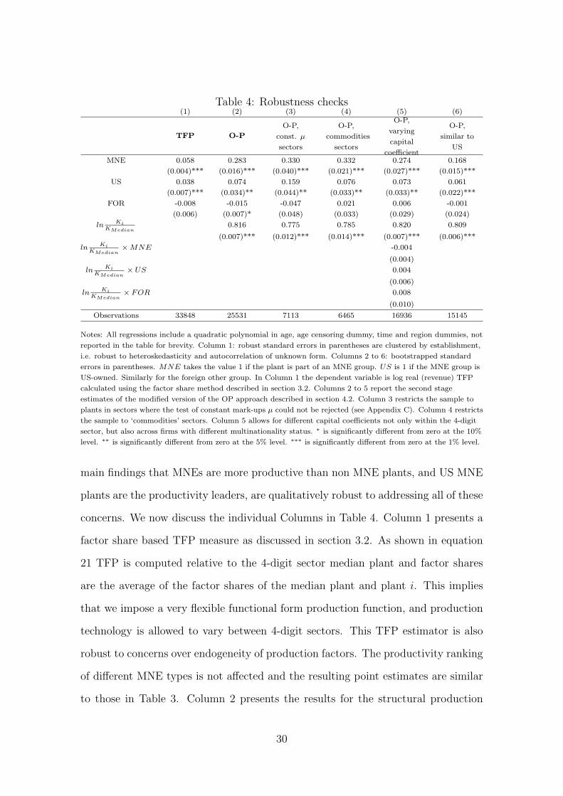
Table 4: Robustness checks(1) (2) (3) (4) (5) (6)

TFP O-P

O-P,

const. µ

sectors

O-P,

commodities

sectors

O-P,

varying

capital

coefficient

O-P,

similar to

US

MNE 0.058 0.283 0.330 0.332 0.274 0.168

(0.004)*** (0.016)*** (0.040)*** (0.021)*** (0.027)*** (0.015)***

US 0.038 0.074 0.159 0.076 0.073 0.061

(0.007)*** (0.034)** (0.044)** (0.033)** (0.033)** (0.022)***

FOR -0.008 -0.015 -0.047 0.021 0.006 -0.001

(0.006) (0.007)* (0.048) (0.033) (0.029) (0.024)

ln KiKMedian

0.816 0.775 0.785 0.820 0.809

(0.007)*** (0.012)*** (0.014)*** (0.007)*** (0.006)***

ln KiKMedian

×MNE -0.004

(0.004)

ln KiKMedian

× US 0.004

(0.006)

ln KiKMedian

× FOR 0.008

(0.010)

Observations 33848 25531 7113 6465 16936 15145

Notes: All regressions include a quadratic polynomial in age, age censoring dummy, time and region dummies, not

reported in the table for brevity. Column 1: robust standard errors in parentheses are clustered by establishment,

i.e. robust to heteroskedasticity and autocorrelation of unknown form. Columns 2 to 6: bootstrapped standard

errors in parentheses. MNE takes the value 1 if the plant is part of an MNE group. US is 1 if the MNE group is

US-owned. Similarly for the foreign other group. In Column 1 the dependent variable is log real (revenue) TFP

calculated using the factor share method described in section 3.2. Columns 2 to 5 report the second stage

estimates of the modified version of the OP approach described in section 4.2. Column 3 restricts the sample to

plants in sectors where the test of constant mark-ups µ could not be rejected (see Appendix C). Column 4 restricts

the sample to ‘commodities’ sectors. Column 5 allows for different capital coefficients not only within the 4-digit

sector, but also across firms with different multinationality status. ∗ is significantly different from zero at the 10%

level. ∗∗ is significantly different from zero at the 5% level. ∗∗∗ is significantly different from zero at the 1% level.

main findings that MNEs are more productive than non MNE plants, and US MNE

plants are the productivity leaders, are qualitatively robust to addressing all of these

concerns. We now discuss the individual Columns in Table 4. Column 1 presents a

factor share based TFP measure as discussed in section 3.2. As shown in equation

21 TFP is computed relative to the 4-digit sector median plant and factor shares

are the average of the factor shares of the median plant and plant i. This implies

that we impose a very flexible functional form production function, and production

technology is allowed to vary between 4-digit sectors. This TFP estimator is also

robust to concerns over endogeneity of production factors. The productivity ranking

of different MNE types is not affected and the resulting point estimates are similar

to those in Table 3. Column 2 presents the results for the structural production

30

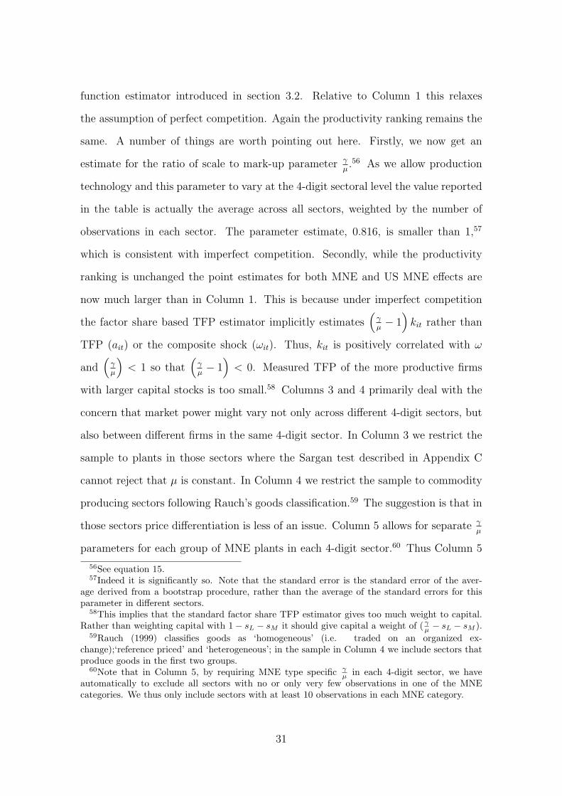
function estimator introduced in section 3.2. Relative to Column 1 this relaxes

the assumption of perfect competition. Again the productivity ranking remains the

same. A number of things are worth pointing out here. Firstly, we now get an

estimate for the ratio of scale to mark-up parameter γµ.56 As we allow production

technology and this parameter to vary at the 4-digit sectoral level the value reported

in the table is actually the average across all sectors, weighted by the number of

observations in each sector. The parameter estimate, 0.816, is smaller than 1,57

which is consistent with imperfect competition. Secondly, while the productivity

ranking is unchanged the point estimates for both MNE and US MNE effects are

now much larger than in Column 1. This is because under imperfect competition

the factor share based TFP estimator implicitly estimates(

γµ− 1

)kit rather than

TFP (ait) or the composite shock (ωit). Thus, kit is positively correlated with ω

and(

γµ

)< 1 so that

(γµ− 1

)< 0. Measured TFP of the more productive firms

with larger capital stocks is too small.58 Columns 3 and 4 primarily deal with the

concern that market power might vary not only across different 4-digit sectors, but

also between different firms in the same 4-digit sector. In Column 3 we restrict the

sample to plants in those sectors where the Sargan test described in Appendix C

cannot reject that µ is constant. In Column 4 we restrict the sample to commodity

producing sectors following Rauch’s goods classification.59 The suggestion is that in

those sectors price differentiation is less of an issue. Column 5 allows for separate γµ

parameters for each group of MNE plants in each 4-digit sector.60 Thus Column 5

56See equation 15.57Indeed it is significantly so. Note that the standard error is the standard error of the aver-

age derived from a bootstrap procedure, rather than the average of the standard errors for thisparameter in different sectors.

58This implies that the standard factor share TFP estimator gives too much weight to capital.Rather than weighting capital with 1− sL − sM it should give capital a weight of ( γ

µ − sL − sM ).59Rauch (1999) classifies goods as ‘homogeneous’ (i.e. traded on an organized ex-

change);‘reference priced’ and ‘heterogeneous’; in the sample in Column 4 we include sectors thatproduce goods in the first two groups.

60Note that in Column 5, by requiring MNE type specific γµ in each 4-digit sector, we have

automatically to exclude all sectors with no or only very few observations in one of the MNEcategories. We thus only include sectors with at least 10 observations in each MNE category.

31

also addresses the concern that results might be driven by MNEs being active in very

different sectors of the economy. As shown by the estimates this is not the case. Also

note that the average values for γµ

for different MNE types reported in rows 4 to 7 of

Column 5 suggest that there are no significant differences in this parameter across

MNE groups. Again the productivity ranking remains qualitatively unchanged.

In Column 6 we address the issue of within 4-digit sector plant heterogeneity by

restricting the regression sample to those plants that are more similar to US MNEs

according to a range of characteristics including labour and material shares, size and

age.61 This again leads to the same qualitative results. To summarize, the results

shown in Table 3 seem to be robust. In the next section we shed more light on the

factors that drive these differences.62

4.3 Explaining the US productivity leadership

Table 5 shows results from the double fixed effects approach described in section

3.3. Column 1 reports estimates from the two stages on the full sample when we

control separately for US MNEs and other foreign effects, with dummies constructed

as MNEeverJ and MNEever

i . We also introduce a set of dummy variables equal to 1

if a plant was set up as a greenfield investment during our sample period by either

a domestic or an MNE firm.63 This controls for the possibility that any best firm

effects – i.e. the transfer of knowledge or technology from MNE parents to their

plants – could be fully realized only in plants set up as greenfields rather than in

takeovers. Row 1 of Column 1 reports the coefficient βMNE estimated in the first

61We construct this subsample by running a probit model where the left hand side variable isthe probability of being US owned and as explanatory variables we include polynomials in labourshare, material share, employment, capital and age. A plant is then considered to be similar to aUS plant if its predicted probability exceeds the median predicted probability value in the sample.

62Other unreported robustness checks include weighted regressions and regressions that controlfor unobserved skill levels in the firm. In terms of the latter, we include in equation 2 averagewages as a proxy for the average skill level of workers; in contrast to other studies (e.g. Griffith andSimpson (2001)) we cannot further distinguish between operatives’ and administrative employees’average wages because this information was not reported in the ARD after 1996.

63The reference category for this set of dummy variables is the plants that were set up beforeour sample started so that we do not know who set them up.

32

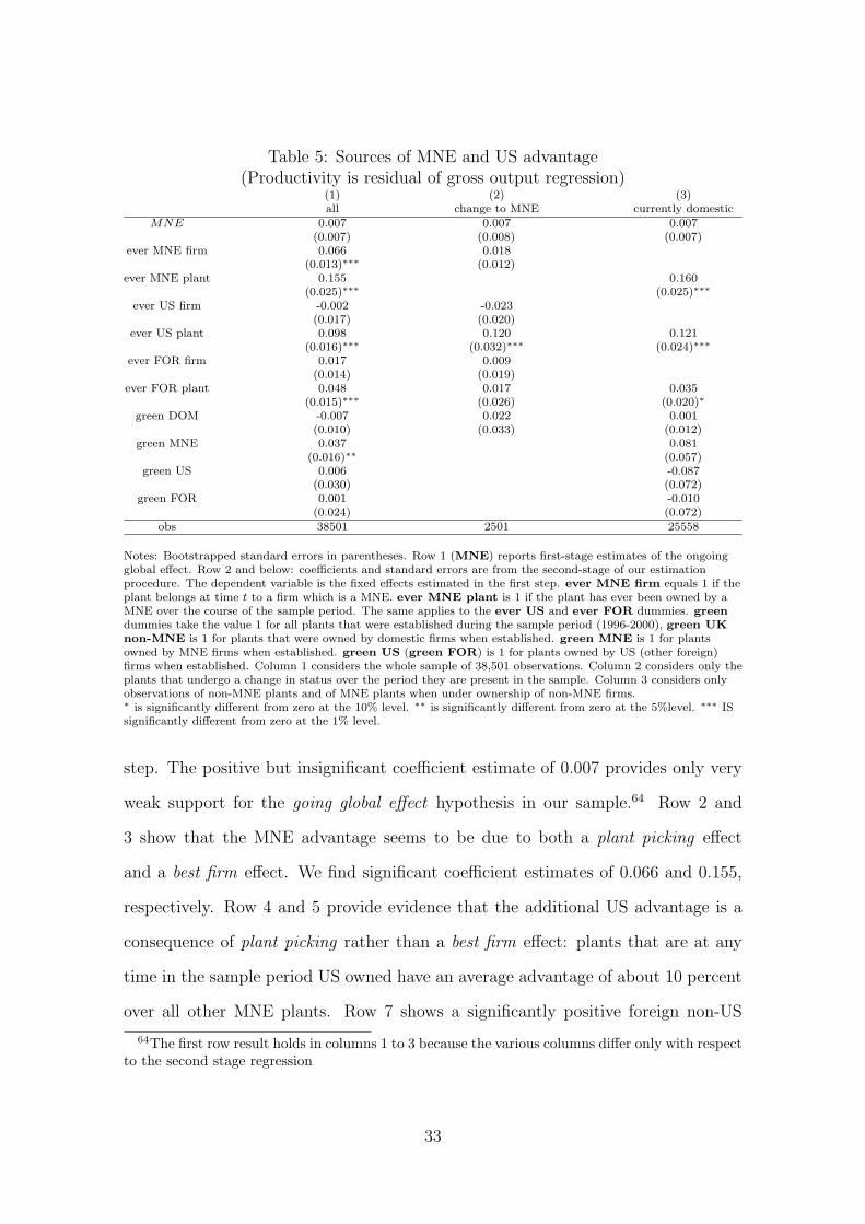
Table 5: Sources of MNE and US advantage(Productivity is residual of gross output regression)

(1) (2) (3)all change to MNE currently domestic

MNE 0.007 0.007 0.007(0.007) (0.008) (0.007)

ever MNE firm 0.066 0.018(0.013)∗∗∗ (0.012)

ever MNE plant 0.155 0.160(0.025)∗∗∗ (0.025)∗∗∗

ever US firm -0.002 -0.023(0.017) (0.020)

ever US plant 0.098 0.120 0.121(0.016)∗∗∗ (0.032)∗∗∗ (0.024)∗∗∗

ever FOR firm 0.017 0.009(0.014) (0.019)

ever FOR plant 0.048 0.017 0.035(0.015)∗∗∗ (0.026) (0.020)∗

green DOM -0.007 0.022 0.001(0.010) (0.033) (0.012)

green MNE 0.037 0.081(0.016)∗∗ (0.057)

green US 0.006 -0.087(0.030) (0.072)

green FOR 0.001 -0.010(0.024) (0.072)

obs 38501 2501 25558

Notes: Bootstrapped standard errors in parentheses. Row 1 (MNE) reports first-stage estimates of the ongoingglobal effect. Row 2 and below: coefficients and standard errors are from the second-stage of our estimationprocedure. The dependent variable is the fixed effects estimated in the first step. ever MNE firm equals 1 if theplant belongs at time t to a firm which is a MNE. ever MNE plant is 1 if the plant has ever been owned by aMNE over the course of the sample period. The same applies to the ever US and ever FOR dummies. greendummies take the value 1 for all plants that were established during the sample period (1996-2000), green UKnon-MNE is 1 for plants that were owned by domestic firms when established. green MNE is 1 for plantsowned by MNE firms when established. green US (green FOR) is 1 for plants owned by US (other foreign)firms when established. Column 1 considers the whole sample of 38,501 observations. Column 2 considers only theplants that undergo a change in status over the period they are present in the sample. Column 3 considers onlyobservations of non-MNE plants and of MNE plants when under ownership of non-MNE firms.∗ is significantly different from zero at the 10% level. ∗∗ is significantly different from zero at the 5%level. ∗∗∗ ISsignificantly different from zero at the 1% level.

step. The positive but insignificant coefficient estimate of 0.007 provides only very

weak support for the going global effect hypothesis in our sample.64 Row 2 and

3 show that the MNE advantage seems to be due to both a plant picking effect

and a best firm effect. We find significant coefficient estimates of 0.066 and 0.155,

respectively. Row 4 and 5 provide evidence that the additional US advantage is a

consequence of plant picking rather than a best firm effect: plants that are at any

time in the sample period US owned have an average advantage of about 10 percent

over all other MNE plants. Row 7 shows a significantly positive foreign non-US

64The first row result holds in columns 1 to 3 because the various columns differ only with respectto the second stage regression

33

plant effect of 4.8 percent, which is lower than the US plant effect.

Finally, rows 8 to 11 report ‘greenfield’ effects. Row 9 shows that plants that

are set up by MNEs enjoy a 3.7 percent advantage relative to non-greenfield domes-

tic plants, significant at the 5 percent level; row 10 and 11 show that there is no

additional advantage from being set up by a US or a foreign MNE.

What could be a potential concern with our estimates in column 1? Firstly, the

estimated multinational best firm effects coefficients are calculated as a weighted

average of all observations of plants currently owned by an MNE firm minus a

weighted average of observations of all plants that are not owned by a MNE firm.

Thus, the MNE firm coefficient,65 βeverJ , could be high for two reasons: if plants which

are owned by multinationals throughout the sample period are very productive66 or

if plants which change their ownership over the course of our sample had a strong

increase in productivity after being taken over by an MNE.67 To get an idea of the

time span that MNEs firms need to increase the productivity of the acquired plants

after takeover68 in column 2 we restrict our sample for the second stage regression

to MNE plants which had a transition from domestic to MNE over the course of our

sample.69 The MNE firm dummy reduces to less than a third relative to column

1, from 0.066 to a borderline significant 0.018. This sharp drop in the magnitude

and significance of the MNE firm effect suggests that improving the productivity

of acquired plants might take some time. In unreported results (available from

the authors) we explore this issue in more detail and found that if we restrict the

analysis to plants that we can observe for at least two years after takeover, i.e. to

65i.e. in terms of the example in Figure 2 in Appendix D, the best firm effect is calculatedas Weighted Average {2t+1, 3t, 3t+1, 4t, 5t, 5t+1, 6t, 6t+1}− Weighted Average {1t, 1t+1, 2t, 4t+1}where (i, t) denotes a plant-year tuple.

66such as 3, 5 and 6 in the example in Figure 2 in Appendix D.67Such as 2 in our example; also if plants such as 4 had a dramatic drop in productivity after

being sold off.68In our example, a particular characteristic of plants such as 5 and 6 is that they have been

owned by a MNE for longer than plants such as 2. Since we have a sample period of 5 years andfor plants such as 2 we must observe at least one takeover, the longest time such a plant could beowned by a MNE is 4 years.

69Like plant 2 in our example.

34

692 observations, the magnitude of the MNE firm dummy coefficient increases to

0.035, but is less precisely estimated with a bootstrapped standard error of 0.022.

The next table presents this issue in more detail.

Secondly, the estimated MNE plant picking effects coefficients are computed as

the weighted average of all observations from MNEever plants minus a weighted

average of all observations from non MNEever plants.70 This plant picking effect

estimate might be upward biased since the estimation includes observations from pe-

riods in which some of the ‘cherry-picked’ plants were owned by an MNEever firm.71

Therefore to check the robustness of the plant picking effects estimates in Column

3 we restrict the second stage regression sample to observations in the years where

all plants (including those that are at some point in time owned by an MNEever

firm) are owned by non-MNE firms.72 Similar to Column 1 Column 3 shows strong

MNE and US plant picking effects suggesting that MNEs, and especially US MNEs,

choose the better plants. In contrast to Column 1, we cannot find an additional

plant picking effect for plants that are taken over by non-US foreign firms.

Finally, a strong assumption in our identification strategy is that all unobserved

heterogeneity affecting MNEs’ selection of plants can be controlled for by non-time

varying fixed effects. However, it is possible that MNEs are more likely to take

over plants following a temporary negative shock - which makes these plants more

vulnerable to hostile takeovers but is un-related to their long-term productivity

potential (scenario 1), or following a positive productivity shock, e.g. an innovation

that would be indicative of better future growth potential for these plants (scenario

2).

Either of these cases can be accounted for using the extension to our structural

70Note that a similar argument holds for US and other foreign plant pick-ing effects. In terms of our example, the plant picking effect is calculated asWeightedAverage{2t, 2t+1, 3t, 3t+1, 5t, 5t+1, 6t, 6t+1} −WeightedAverage{1t, 1t+1, 4t, 4t+1}.

71In terms of the example these are (2, t + 1) and (4, t).72i.e. we identify the plant effect from WeightedAverage{(2, t)} −

WeightedAverage{(1, t), (1, t + 1), (4, t + 1)}.

35

productivity estimation framework introduced in section 3.3.2. Before discussing

the results it is worth noting that only scenario 2 could undermine the conclusion

that the estimated US advantage over other MNEs is due to plant picking rather

than firm effects. This is because in scenario 1 the double fixed effects set-up would

lead to an overestimation of any firm effects. Scenario 2 on the other hand would

lead to an underestimation of firm effects in the double fixed effects case and could

therefore explain why we fail to find any additional US firms effects.

In Table 6 we report the results from the structural model extension from section

3.3.2. We make a number of simplifying assumptions based on the results so far;

but it should be noted that our framework does not depend on these assumptions.

For instance, we no longer let the capital coefficient – γµ

vary across sectors.

Column 1 simply replicates the OP style regression from Table 4 with constant

γµ. Our results of large MNE and larger US MNE effects remain. Secondly, since in

the double fixed effects case where we did not find much evidence of a going global

effect, we no longer allow for this in this setting. This reduces the dimensionality of

the selection model that we are adding to the structural framework. Column 2 of

Table 6 shows the results from allowing a selection model where only ωit−1 enters the

equation determining takeover in period t. We find: firstly, that any additional US

effect vanishes while a general MNE effect persists; secondly, rows 5 to 7 show that

for all three types of MNEs the coefficients on ωit−1 from the selection equations73 are

positive and significant. Thus, MNEs select firms that were more productive in the

period before takeover. Moreover, note that the selection coefficient is higher, and

significantly so, as the t value in row 12 reveals – for US firms. Column 3 includes

both ωit−1 and the average of ω before takeover ωit−1. In this set-up the coefficient

on ωit−1 captures the importance solely of short term effects.74 None of the short-

term coefficients is significant. The long-term average coefficients are similar in size

73Compare with equation 34.74The previous Column ωit−1 in the absence of any other control, captured a combination of

short and long run effects.

36

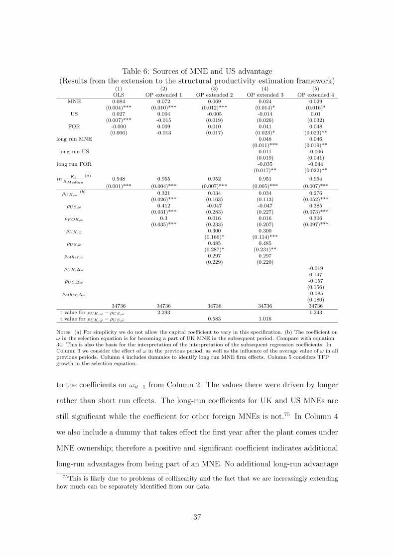
Table 6: Sources of MNE and US advantage(Results from the extension to the structural productivity estimation framework)

(1) (2) (3) (4) (5)OLS OP extended 1 OP extended 2 OP extended 3 OP extended 4

MNE 0.084 0.072 0.069 0.024 0.029(0.004)*** (0.010)*** (0.012)*** (0.014)* (0.016)*

US 0.027 0.004 -0.005 -0.014 0.01(0.007)*** -0.015 (0.019) (0.026) (0.032)

FOR -0.000 0.009 0.010 0.041 0.048(0.006) -0.013 (0.017) (0.023)* (0.023)**

long run MNE 0.048 0.046(0.011)*** (0.019)**

long run US 0.011 -0.006(0.019) (0.041)

long run FOR -0.035 -0.044(0.017)** (0.022)**

ln KiKMedian

(a)0.948 0.955 0.952 0.951 0.954

(0.001)*** (0.004)*** (0.007)*** (0.005)*** (0.007)***

ρUK,ω(b) 0.321 0.034 0.034 0.276

(0.026)*** (0.163) (0.113) (0.052)***ρUS,ω 0.412 -0.047 -0.047 0.385

(0.031)*** (0.283) (0.227) (0.073)***ρFOR,ω 0.3 0.016 0.016 0.306

(0.035)*** (0.233) (0.207) (0.097)***ρUK,ω 0.300 0.300

(0.166)* (0.114)***ρUS,ω 0.485 0.485

(0.287)* (0.231)**ρother,ω 0.297 0.297

(0.229) (0.220)ρUK,∆ω -0.019

0.147ρUS,∆ω -0.157

(0.156)ρother,∆ω -0.085

(0.180)34736 34736 34736 34736 34736

t value for ρUK,ω − ρUS,ω 2.293 1.243t value for ρUK,ω − ρUS,ω 0.583 1.016

Notes: (a) For simplicity we do not allow the capital coefficient to vary in this specification. (b) The coefficient onω in the selection equation is for becoming a part of UK MNE in the subsequent period. Compare with equation34. This is also the basis for the interpretation of the interpretation of the subsequent regression coefficients. InColumn 3 we consider the effect of ω in the previous period, as well as the influence of the average value of ω in allprevious periods. Column 4 includes dummies to identify long run MNE firm effects. Column 5 considers TFPgrowth in the selection equation.

to the coefficients on ωit−1 from Column 2. The values there were driven by longer

rather than short run effects. The long-run coefficients for UK and US MNEs are

still significant while the coefficient for other foreign MNEs is not.75 In Column 4

we also include a dummy that takes effect the first year after the plant comes under

MNE ownership; therefore a positive and significant coefficient indicates additional

long-run advantages from being part of an MNE. No additional long-run advantage

75This is likely due to problems of collinearity and the fact that we are increasingly extendinghow much can be separately identified from our data.

37

derives from being part of a US multinational. Finally, in Column 5 we include both

level of ωit−1 and its lagged growth rate; this latter should capture whether changes

in productivity rather than levels are driving the decision of MNE firms to take over

particular plants. The growth term is never significant. In all of these cases, the key

conclusion that there are no additional US firm effects once selection is controlled

for, holds.

5 Conclusions

This study looks at the reasons behind aggregate US productivity leadership by

examining the performance of US MNEs in the UK relative to the performances of

UK MNEs and other foreign MNEs. This allows us to identify to what extent US

productivity leadership is driven by firm specific technological factors rather than

factors that are specific to the business environment in the US.

Compared to earlier studies, we are able to identify UK MNEs in such an analysis.

Thus, we are able to control for the potential bias that arises because in any country

MNEs are a self-selected group of top firms.

Our analysis confirms and qualifies an earlier study by Doms and Jensen (Doms

and Jensen, 1998) using US data, which ranks US MNEs highest followed by other

MNEs, with domestic firms ranked lowest. However, in their case it cannot be ruled

out that the leadership of US multinationals is simply the consequence of a home

advantage. Our results suggest that this ranking is not driven by a home market

advantage for US firms.

In fact, we find that US owned plants have a significant productivity advantage

in the UK, relative to both British MNE and other foreign owned plants, which show

similar productivity levels and are both more productive than plants that do not

invest abroad. This result is robust to imperfect competition, non-constant returns

to scale and differences in flexible production technologies across 4-digit sectors and

38

different types of firms.

Using the dynamic variation in our data we address the concern that US produc-

tivity leadership might be driven by the selection in the takeover process of superior

plants, rather than by technology and knowledge transfers from MNE parent com-

panies to their subsidiaries. We find evidence for both US MNE firm effects and

plant selection effects. However, firm effects are as strong for US MNEs as for other

MNE firms, but the takeovers by US MNEs tend to target plants at the top of the

productivity spectrum. We conclude therefore that the US productivity lead found

in the level regressions is driven mainly by these stronger picking effects.

There could be some concern in relation to the short time period of our sample

in that if firm effects take some time to materialise they would not be detected in

our study. Although we cannot exclude the possibility that if we had a longer panel

we might find stronger firm effects, the fact that we actually find strong MNE firm

effects occurring soon after an MNE takeover (except that they are not any stronger

for US firms) gives us some confidence that a longer time span would not change

the qualitative ranking.

Our results have a number of implications.

Firstly, they suggest that aggregate US productivity leadership might be driven

by factors other than technology, i.e. that other factors are driving the aggregate

gap. An interesting hypothesis is that well functioning competitive markets in the

US76 are more efficient at allocating larger market shares to more productive plants.

Because aggregate productivity is the sum of each firm’s productivity weighted by

its market share, this better selection mechanism results in higher aggregate pro-

ductivity.77

Secondly, in terms of UK economic policy where there is a widely held view

76This is the conclusion of Lewis (2004) on the basis of an impressive number of case studies.77To answer this question thoroughly we would need comparable UK and US micro data. Al-

though beyond the scope of this paper efforts are under way to make progress in this area, see forexample Bartelsman et al. (2003).

39

that incentives for foreign MNEs to locate in Britain are a potential instrument

to increase aggregate productivity performance, our results suggest that attracting

specifically US FDI is unlikely to provide a quick fix for productivity problems.

Thirdly, while we cannot find any evidence that US MNEs are better at trans-

ferring knowledge and technology to their subsidiaries, we did find evidence that

they are better at choosing the best plants to take over. Why should US firms be

better than all other MNEs at selecting the best plants? There are several possi-

ble reasons. One hypothesis is that managers of US MNEs pursue more aggressive

takeover strategies and have specific skills that make them more successful in this

activity. A second explanation is related to the particular time period considered.

Indeed, in the second half of the 1990s, the US Stock market experienced a boom

accompanied by spectacular equity price increases. During that period, the S&P500,

the Dow Jones Industrial and the NASDAQ Composite indices more than doubled.

US MNEs, overvalued in the US stock market, and thus with access to low cost cap-

ital, might have found it more profitable to use this capital to target firms abroad

(e.g. in the UK) not affected by the same stock market bubble, rather than in the

home country.78 From our data it is not possible to thoroughly investigate these

hypotheses, but this is an area of research that deserves further exploration.

References

Arellano, M. and Bond, S. R. (1991). Some tests of specification for panel data:

Monte Carlo evidence and an application to employment equations. Review of

Economic Studies, 58:277–297.

Baily, M. N., Hulten, C., and Campbell, D. (1992). Productivity dynamics in man-

ufacturing plants. Brookings Papers: Microeconomics, pages 187–267.

78This is the ‘cheap capital’ view of FDI (Baker et al., 2004)

40

Baker, M., Foley, C. F., and Wurgler, J. (2004). The stock market and investment:

Evidence from FDI flows. NBER Working Paper, 10559.

Bartelsman, E., Scarpetta, S., and Schivardi, F. (2003). Comparative analysis of

firm demographics and survival: micro-level evidence for the OECD countries.

OECD Economics department working paper, (348).

Blundell, R. and Bond, S. (1998). Initial conditions and moment restrictions in

dynamic panel data models. Journal of Econometrics, 87:115–143.

Branstetter, L. (2001). Are knowledge spillovers international or intranational in

scope? microeconometric evidence from the United States and Japan. Journal of

International Economics, 53:53–79.

Criscuolo, C., Haskel, J., and Martin, R. (2003). Building the evidence base for

productivity policy using business data linking. Economic Trends, 600:39–51.

Criscuolo, C. and Martin, R. (2003). Using the Annual Inquiry into Foreign Direct

Investment to create a multinational identifier in the ARD. Ceriba data guide.

Dixit, A. K. and Stiglitz, J. E. (1977). Monopolistic competition and optimum

product diversity. American Economic Review, 67:297–308.

Doms, M. E. and Jensen, J. B. (1998). Comparing wages, skills and productiv-

ity between domestically and foreign-owned manufacturing establishments in the

United States. In Robert E. Baldwin, R. E. L. and Richardson, J. D., editors,

Geography and Ownership as bases for economic accounting, pages 235–258. Uni-

versity of Chicago.

Dunning, J. H. (1981). International Production and the Multinational Enterprise.

George Allen and Unwin.

Foster, L., Haltiwanger, J. C., and Syverson, C. (2003). Reallocation, firm turnover,

and efficiency: Selection on productivity or profitability? working paper.

41

Griffith, R. (1999). Using the ARD establishment level data to look at foreign

ownership and productivity in the UK. Economic Journal, 109:F416–F442.

Griffith, R. and Simpson, H. (2001). Characteristics of foreign owned firms in British

manufacturing. IFS Working Paper.

Griliches, Z. and Mairesse, J. (1995). Production functions: The search for identifi-

cation. NBER Working Paper, (5067).

Hajivassiliou, V. and Ruud, P. A. (1993). Classical estimation methods for

LDV models using simulation. Econometrics 9311002, EconWPA. available at

http://ideas.repec.org/p/wpa/wuwpem/9311002.html.

Harris, R. (1999). Efficiency in UK manufacturing 1974-1994. mimeo.

Helpman, E. (1984). A simple theory of international trade with multinational

corporations. Journal of Political Economy, 92:451–477.

Helpman, E., Melitz, M. J., and Yeaple, S. R. (2004). Export versus FDI with

heterogenous firms. American Economic Review, 94(1):300–316.

Katayama, H., Lu, S., and Tybout, J. (2003). Why plant-level productivity studies

are often misleading, and an alternative approach to interference. NBER Working

Paper, (9617).

Keller, W. (2004). International technology diffusion. Journal of Economic Litera-

ture, 42:752–782.

Klette, T. J. (1999). Market power, scale economies and productivity: esti-

mates from a panel of establishment data. Journal of Industrial Economics,

XLVII(4):451–476.

42

Klette, T. J. and Griliches, Z. (1996). The inconsistency of common scale esti-

mators when output prices are unobserved and endogenous. Journal of Applied

Econometrics, 11:343–361.

Levinsohn, J. and Petrin, A. (2000). Estimating production functions using inputs

to control for unobservables. NBER Working Paper, (7819).

Levinsohn, J. and Petrin, A. (2003). Estimating production functions using inputs

to control for unobservables. Review of Economic Studies, 70(2):317–342.

Lewis, W. (2004). The power of productivity. The University of Chicago Press.

Markusen, J. R. (1995). The boundaries of multinational enterprises and the theory

of international trade. Journal of Economic Perspectives, 9(2):169–186.

Martin, R. (2002). Building the capital stock. CeRiBA mimeo.

Martin, R. (2003). Computing the true spread. CEP Discussion Paper 0692.

Melitz, M. J. (2000). Estimating firm-level productivity in differentiated product

industries. working paper.

Office for National Statistics (2002). Foreign Direct Investment 2000 - Business

Monitor MA4. HMSO, London.

Olley, S. and Pakes, A. (1996). The dynamics of productivity in the telecomunica-

tions equipment industry. Econometrica, 64:1263–97.

O’Mahony, M. and de Boer, W. (2002). Britain’s relative productivity performance:

updates to 1999. Final report to DTI/HM Treasury/ONS, NIESR.

O’Mahony, M. and van Ark, B. (2003). EU productivity and competitiveness: An

industry perspective. Office for Official Publications of the European Communities.

43

Oulton, N. (1997). The ABI Respondents Database: A new resource for industrial

economics research. Economic Trends, 528:46–57.

Oulton, N. (2000). Why do foreign-owned firms in the UK have higher labour

productivity? Bank of England.

Rauch, J. (1999). Network vs markets in international trade. Journal of Interna-

tional Economics, 48(1):7–35.

Syverson, C. (2004). Market structure and productivity: A concrete example. Jour-

nal of Political Economy, 112(6):1181–1222.

Wagner, K. and van Ark, B. E. (1996). International Productivity Differences,

Measurement and Explanations. North-Holland.

A Variables Definitions

• Capital stock: capital stock was calculated using a perpetual inventory method

(PIM). For a more detailed description of the method adopted we refer to

Martin (2002).

• Deflators: to deflate output measures (gross output and value added) we use

producer price indices (PPI) at the 4-digit SIC92 industry level. To deflate

intermediates, we use material price deflators at the 2-digit SIC92 industry

level. The base year is 1995. Capital stock is deflated using investment de-

flators with base year 1995; for years pre-1995 these are implicitly derived

from nominal and real sectoral ONS historical investment series. From 1995

onwards we use the publicly available MM17 series.

• Foreign plants are plants owned by foreign owned enterprise groups.

• Country groups:

44

EU includes plants owned by Austria, Belgium, Denmark, Finland, Luxem-

bourg, Sweden, the Republic of Ireland, Italy, Spain and the Canary

Islands, Portugal, and Greece.

non-EU includes plants owned by British Virgin Islands, Channel Islands,

Isle of Man, Liechtenstein, Antigua and Barbuda, Cyprus, US Virgin Is-

lands, Norway, Switzerland, Australia, Canada, Czech Republic, Iceland,

Mexico, Poland, South Korea and Turkey and plants owned by the rest

of the world and plants that are foreign owned, but whose nationality is

unknown.

• Weights are calculated using the employment register information on the basis

of 4 digit sector, region and employment cells. For each cell i the weight is

calculated as Number of plants in register in cell iNumber of selected plants cell i

.

B The monotone relationship between profits and

shocks

Start by noting that given our assumption of a homogenous production function

(equation 3) we can write the cost minimization problem as:

C(Kit,wV it) = minXV it

∑

z 6=K

wzitXzit s.t. 1 = f(Kit, XV it

)(40)

where wzit represents the cost of factor z and Kit = Kit

Qitwith Qit =

(Qit

Ait

) 1γ. XV it

collects the same transformation for all variable production factors in a vector. Total

costs become in terms of Equation 40

Cit = CitQit (41)

45

Next consider the profit function.

Πit(Kit, λit, ait,wit) = Rit − Cit

Given the demand function 5 and the cost function 41 we can write it as

Πit(Kit, λit, ait,wit) =

(ΛitRt

Pt

) 1η

PtQ1− 1

η − CitQit (42)

Note that the firm’s profit maximization first order condition is

(1− 1

η

)Rit

Qit

=1

γz(Qit, Kit)

Qit

Qit

(43)

where

z(Qit, Kit) =∂Cit

∂Qit

Qit + Cit (44)

Finally, note that the derivatives of profits with respect to λit and ait are

∂Πit

∂λit

= µ−1Rit

and

∂Πit

∂ait

= z(Qit, Kit)1

γ

(Qit

Ait

) 1γ

= µ−1Rit (45)

where applying the envelope theorem the last equality follows from the first order

condition 43. and

µ =

(1− 1

η

)−1

As a consequence of all these results we get for the total differential of profits

dΠit = Rit1

µ(dλit + dait) = Ritdωit (46)

which establishes that there is a positive relationship between profits and the com-

46

posite shock index ωit.

C Testing if µ is constant

In this section, we describe a simple test based on over-identifying restrictions of

the hypothesis that µ is constant within each 4-digit sector. As expected, the null

hypothesis is rejected in the majority of sectors. Column 3 of Table 3 shows estimates

of equation 20 for a restricted sample of plants in those sectors where the null

hypothesis of constant µ cannot be rejected to check the robustness of our results.

Our test works as follows. To allow for a more general market structure we let the

coefficient of capital in equation 18 depend on the demand shock of the firm, λit.79

rit − viit = βKit kit + g(kit−1, Πit−1) + νit (47)

where βKit = γ

µitand µit = µ(λit−1). Note that we assume that markups depend only

on lagged values of λit. We require this assumption for our test. One can motivate

it by a certain sluggishness in price setting. To understand our next steps suppose

that we had a way of observing λit−1 but are ignorant about the shape of the markup

function µ(·). To estimate 47 we can approximate βKit by yet another polynomial

expansion in λ. Thus in the regression we would get interactions between kit and the

polynomials terms as extra explanatory variables; e.g. kit×λ2it−1. If we assume that

markups and thus βK ’s are constant across firms on the other hand, we can use zero

moment conditions between these interaction terms and the residuals as additional

moment conditions – e.g. E{νit × kit × λ2it−1} = 0 – to identify the reduced set of

parameters of the constant markup model. The problem with this strategy is that

λ is not observed. Notice however that80 a necessary implication of these additional

79For simplicity we make the formal argument in terms of log levels and not deviations from logvalues of the median plant as in section 3.2. A similar argument can be made in both cases.

80Unless demand shocks λ and technical TFP shocks ait are perfectly negatively correlated thatis

47

moment conditions is that the interaction terms are not correlated with ω = either;

e.g E{νit× kit×ω2it−1} = 0 Thus to examine if these additional moment restrictions

are valid we need estimates of νit and ωit−1. We described above how we can derive

those.

D Identification of double fixed effects

Figure 2: An example

� � �

� � � � � �

� � �

� ��� � �

� � � �

� � � � �

Suppose our sample consists of 6 plants81 which are owned by 3 different firms

(A, B and C). We observe them for two periods, t and t+1. In period t firms A and

B are domestic, while firm C is an MNE. In period 2 firm B starts investing abroad

and thus becomes an MNE whereas A remains domestic.82 Moreover, we have the

following takeover events: plant 2 is acquired by C and plant 4 is sold off to firm A

by firm B before it starts investing abroad.83 How can we differentiate between the

MNE effects discussed in the paper with the variation in this example? Consider

first the plant picking effect. The plant in the example that was taken over by an

81numbered 1 to 6 in figure 282In terms of our earlier dummies we would thus have MNEever

A = 0, MNEeverB = 1 (both, in

year t and t+1) and MNEeverC = 1

83Consequently MNEever1 = 0 and MNEever

4 = 0 whereas for all other plants MNEeveri = 1

∀i = 2, 3, 5, 6.

48

MNE is plant 2. If we found that in year t plant 2 had a higher productivity than

plant 1 this would be evidence of a plant picking effect. To examine the existence

of best firm effects we can compare the productivity of plant 2 in year t + 1 relative

to year t. If its productivity increases after it is taken over by firm C this would be

evidence of a best firm effect.84 Finally, for the going global effect we need to look

at firm B and examine whether the productivity of its plant 3 increases from t to

t + 1.

In our sample, how many changes between multinational Status for firms and

between different types of firms for plants, do we observe? Table 7 reports the

occurrence of all these changes in our dataset. The upper panel reports the number

of status changes for each possible transition between UK non-MNE, UK MNEs, US

MNEs and non-US Foreign MNEs (FOR). For example the cell in row 1, Column

2 reports that in our sample there are 589 transitions from UK non-MNEs to UK

MNEs. The lower panel reports only the number of status changes that also involve

an ownership change. Therefore, the cell in row 5 Column 2 reports that 255 of

the 589 British plants that became multinational did so by means of an ownership

change, i.e. a takeover. This implies that the remaining 334 plants became part of

a British MNE because the firm they belonged to started investing abroad. This is

the variation we use to identify βMNE. In total, the upper panel shows that we have

1,118 changes between non-MNE and MNE status.85 The lower panel shows that

784 of these changes involved a change in ownership, i.e. a takeover. Overall, panel

1 of Table 7 shows that about 10% of all the transition events we observe in the data

involve a change in multinational status.86 From panel 2 we can derive that about

40% of all ownership changes in our sample involve changes between multinational

84Equally, we could see whether the productivity of plant 4 decreases once it is taken over by Ain period t + 1.

85We obtain this figure by summing the off diagonal elements of row 1 and Column 1 in theupper panel.

86This is computed as the share of all off diagonal elements to the sum of all cells in table 7.

49

status.87 Thus, while the majority of plants do not change status, in the data there

is still some non-negligible number of status changes.

Table 7: Status changes in the data(Transitions in ownership and MNE status in sample 1996-2000)

(1) (2) (3) (4)UK non MNE UK MNE US FOR

Status changesUK Non MNE 11164 589 225 304

UK MNE 251 3170 101 46US 155 62 1290 48

FOR 138 42 26 1857Status changes with ownership change

UK Non MNE 1511 255 225 304UK MNE 164 51 101 46

US 155 62 131 48FOR 138 42 26 246

Notes: UKnonMNE denotes domestic plants with no FDI; UKMNE is 1 for all domestic multinationals; US is 1for all plants owned by a US multinational and FOR is 1 for all plants owned by non-US foreign multinationals.Panel one of the table reports the number of plants that change their MNE status; panel two reports the subset ofthese that also experienced an ownership change. For example Row 1 Column 2 reports that there are 589transitions from UK non-MNE to UK MNE. Row 5 Column 2 reports that in 255 cases these transitions alsoinvolved a takeover. The number of observations in the sample is 38,501. The period considered is 1996-2000.Source: Authors’ calculation using the ARD AFDI matched data.

87Again, computed as the share of all off diagonal elements, but this time of panel 2

50