multimode approach to classical and quantum diffraction
TRANSCRIPT
Louisiana State UniversityLSU Digital Commons
LSU Doctoral Dissertations Graduate School
11-15-2017
Multimode Approach to Classical and QuantumDiffractionZhihao XiaoLouisiana State University and Agricultural and Mechanical College, [email protected]
Follow this and additional works at: https://digitalcommons.lsu.edu/gradschool_dissertations
Part of the Physics Commons
This Dissertation is brought to you for free and open access by the Graduate School at LSU Digital Commons. It has been accepted for inclusion inLSU Doctoral Dissertations by an authorized graduate school editor of LSU Digital Commons. For more information, please [email protected].
Recommended CitationXiao, Zhihao, "Multimode Approach to Classical and Quantum Diffraction" (2017). LSU Doctoral Dissertations. 4178.https://digitalcommons.lsu.edu/gradschool_dissertations/4178

MULTIMODE APPROACH TO CLASSICAL AND QUANTUM DIFFRACTION
A Dissertation
Submitted to the Graduate Faculty of theLouisiana State University and
Agricultural and Mechanical Collegein partial fulfillment of the
requirements for the degree ofDoctor of Philosophy
in
Department of Physics and Astronomy
byZhihao Xiao
Bachelor of Science, University of Science and Technology of China, 2008Master of Science, University of Science and Technology of China, 2011
May 2018

To my parents, Prof. Xianbin Xiao and Prof. Yulan Xu.
ii
Acknowledgments
I am extremely grateful to my advisors Dr. Hwang Lee and Dr. Jonathan P. Dowling.
This work could not have been completed without their support and guidance. I particularly
appreciate the patience they showed me when I was building “the ground floor” of this work
which enables me to develop a solid and clear understanding on the subject. The useful
skills and the ways of thinking they have taught me will always be my prized possessions
as they are helpful not only on this work but also other subjects I may choose to study
in future. Besides, the work is certainly made less burdensome by Dr. Dowling’s many
anecdotes and colorful jokes, most of which I find very enjoyable, especially when not having
lunch.
This work is done in collaboration with my fellow student R. Nicholas Lanning and
Drs. Mi Zhang, Irina Novikova, Eugeniy E. Mikhailov, Masahiro Takeoka, Kouichi Semba,
Tomoko Fuse, Sahel Ashhab, Fumiki Yoshihara. It is my pleasure working with them and
I wish our future collaboration will be as productive. I would also like to thank the rest
of my dissertation committee members Dr. Thomas Corbitt, Dr. Daniel Sheehy and Dr.
Michael G. Benton for their time and kind words.
I would also like to acknowledge support from the Army Research Office, the Air
Force Office of Scientific Research (grant FA9550-13-1-0098), the Defense Advance Research
Projects Agency, the National Science Foundation, the Office of Naval Research, and the
Northrop Grumman Corporation.
iii

Table of Contents
ACKNOWLEDGMENTS . . . . . . . . . . . . . . . . . . . . . . . . . . . . . . . . . . . . . . . . . . . . . . . . . . . . . . . . . . iii
ABSTRACT . . . . . . . . . . . . . . . . . . . . . . . . . . . . . . . . . . . . . . . . . . . . . . . . . . . . . . . . . . . . . . . . . . . . . . vi
CHAPTER1 OVERALL INTRODUCTION . . . . . . . . . . . . . . . . . . . . . . . . . . . . . . . . . . . . . . . . . . . . . 1
2 ADVANCING THE PRINCIPLE FOR CLASSICAL OP-TICAL BEAM DIFFRACTION: GAUSSIAN BEAM SPA-TIAL MODES DECOMPOSITION METHOD . . . . . . . . . . . . . . . . . . . . . . . . . . . . . 32.1 Chapter 2 Introduction . . . . . . . . . . . . . . . . . . . . . . . . . . . . . . . . . . . . . . . . . . . . . . . 32.2 Gaussian Beam Modes Decomposition Method . . . . . . . . . . . . . . . . . . . . . . . . 42.3 Numerical Simulation: Comparing Gaussian Beam Modes
Decomposition Method with Kirchhoff’s Diffraction For-mula . . . . . . . . . . . . . . . . . . . . . . . . . . . . . . . . . . . . . . . . . . . . . . . . . . . . . . . . . . . . . . . . . 7
2.4 Chapter 2 Conclusion . . . . . . . . . . . . . . . . . . . . . . . . . . . . . . . . . . . . . . . . . . . . . . . . . 17
3 WHY A HOLE IS LIKE A BEAM SPLITTER: A GEN-ERAL DIFFRACTION THEORY FOR MULTIMODE QUAN-TUM STATES OF LIGHT. . . . . . . . . . . . . . . . . . . . . . . . . . . . . . . . . . . . . . . . . . . . . . . . . 193.1 Chapter 3 Introduction . . . . . . . . . . . . . . . . . . . . . . . . . . . . . . . . . . . . . . . . . . . . . . . 193.2 Classical Electrodynamic Description of Gaussian Beam
Spatial Modes . . . . . . . . . . . . . . . . . . . . . . . . . . . . . . . . . . . . . . . . . . . . . . . . . . . . . . . . 203.3 Quantization of Gaussian Modes . . . . . . . . . . . . . . . . . . . . . . . . . . . . . . . . . . . . . . 253.4 Additional Examples of the Use of the Theory. . . . . . . . . . . . . . . . . . . . . . . . . 313.5 Chapter 3 Conclusion . . . . . . . . . . . . . . . . . . . . . . . . . . . . . . . . . . . . . . . . . . . . . . . . . 52
4 EVOLUTION UNDER HAMILTONIAN WITH TIME-DEPENDENTQUBIT–OSCILLATOR COUPLING . . . . . . . . . . . . . . . . . . . . . . . . . . . . . . . . . . . . . . . 544.1 Chapter 4 Introduction . . . . . . . . . . . . . . . . . . . . . . . . . . . . . . . . . . . . . . . . . . . . . . . 544.2 Evolution under Time–dependent Qubit-oscillator Cou-
pling Coefficient with Infinitesimal Qubit Frequency . . . . . . . . . . . . . . . . . . . 554.3 First Order Correction for Small ∆ . . . . . . . . . . . . . . . . . . . . . . . . . . . . . . . . . . . 624.4 Application of π-pulses . . . . . . . . . . . . . . . . . . . . . . . . . . . . . . . . . . . . . . . . . . . . . . . 674.5 Chapter 4 Conclusion . . . . . . . . . . . . . . . . . . . . . . . . . . . . . . . . . . . . . . . . . . . . . . . . . 724.6 Chapter 4 Supplementary Material: Detailed Deriva-
tion for Evolution under Time–dependent Qubit-oscillatorCoupling Coefficient with Infinitesimal Qubit Frequency.. . . . . . . . . . . . . . . 72
5 OVERALL CONCLUSION . . . . . . . . . . . . . . . . . . . . . . . . . . . . . . . . . . . . . . . . . . . . . . . . 82
REFERENCES . . . . . . . . . . . . . . . . . . . . . . . . . . . . . . . . . . . . . . . . . . . . . . . . . . . . . . . . . . . . . . . . . . . . 84
iv

APPENDIX: PERMISSION . . . . . . . . . . . . . . . . . . . . . . . . . . . . . . . . . . . . . . . . . . . . . . . . . . . . . . . 87
VITA . . . . . . . . . . . . . . . . . . . . . . . . . . . . . . . . . . . . . . . . . . . . . . . . . . . . . . . . . . . . . . . . . . . . . . . . . . . . . 88
v

Abstract
I have investigated classical diffraction of optical beams with multimode approach,
which is a significant improvement upon the traditional Huygens-Fresnel principle based
diffraction theory. I have also investigated quantum diffraction with multimode approach,
which describes the behavior of multimode quantum state. Multimode approach to clas-
sical and quantum diffraction provides a clear mathematical formalism and is verified by
numerical simulations. In addition, I present the work on superconducting qubit and oscil-
lator with time–dependent coupling coefficient, with first order correction with finite qubit
energy and schemes based on and π pulses.
vi

Chapter 1
Overall Introduction
The traditional method of treating an optical beam diffracted through a spatial mask is
based Huygens-Fresnel principle and Kirchhoff’s diffraction formula. However, this method
has some drawbacks since calculations with Kirchhoff’s diffraction formula is usually com-
plicated and computationally intensive. To simplify the calculation, the diffracted field is
divided into near field (known as Fresnel diffraction) and far field (known as Fraunhofer
diffraction), so that certain approximations can be applied. This strategy of separate treat-
ments is far from ideal, in the sense that we are forced to either solve the problem with one
complicated calculation or divide the problem so that the calculation can be simplified but
two separate treatments are required. Additionally, it is no simple solution for the inter-
mediate field (between the near and the far field), and there is no clear picture describing
how the near or the far field would transition into the other.
Presented in Chapter 2 of this dissertation, the multimode approach to this classical
diffraction problem, is developed based on a new angle. Specifically, it is based on the
principle that the source beam and the diffracted beam should have the same boundary
field amplitude at the spatial mask. Compared to Kirchhoff’s diffraction formula and its
approximation, the multimode approach has a neater mathematical structure and simpler
formalism. In practice, the multimode approach also significantly lightens the computa-
tional burden and provides a better and easier mechanism for precision control. Numerical
simulation is employed to demonstrate these advantages of the multimode approach to
classical diffraction. Further exploration is also made to demonstrate the more efficient
way to apply the multimode approach.
Chapter 3. is based on the work done by the author in collaboration with R. Nicholas
Lanning, Mi Zhang, Irina Novikova, Eugeniy E. Mikhailov and Jonathan P. Dowling, and
it is published in Ref. ([1]). For Laser beams the field amplitude as functions of spatial
coordinates are the Gaussian beams modes. However, a large portion of existing mod-
1

els dealing with quantum state of light are treating the lasers as plane waves instead of
Gaussian beams. The advantage of using plane waves to approximate Gaussian beams is
that the former are mathematically simpler. But the disadvantage is that such approxi-
mation requires certain conditions, such as, when the beam waist and Rayleigh range can
be treated as much larger than the typical width and depth of the experiment. However,
such conditions are not always satisfied, which will result in inaccurate approximation.
This leads to experimental data deviating from theoretical prediction and missing poten-
tial findings. Therefore we have developed the quantization of Gaussian beams to address
this problem. The essential component of this work is the transformation of the operators
amongst various Gaussian beam modes, which determines how the multimode quantum
states will evolve and interact.
The quantization of multimode Gaussian beam we developed has opened up new op-
portunities to investigate quantum effect of almost all Gaussian beam based models. The
theoretical prediction derived from numerical simulations qualitatively agrees with our ex-
perimental data published in Ref. ([2]) providing us with strong evidence of the effectiveness
of our method. More theoretical and experimental work related to this subject, which the
author takes part in, are also published in Ref. ([3, 4]).
In Chapter 4, I will present the work on superconducting qubit and oscillator with time–
dependent coupling coefficient g(t), first order correction for small ∆, and π pulses. For the
system of superconducting qubitoscillator circuit in deep strong coupling regime, the energy
ground state and first excited state are both so called the Schrdingers cat states, which
have important applications in both in quantum science and technology such as quantum
communication and computing. My collaborators and I have investigated the evolution of
the quantum state under a changing coupling coefficient, and also have investigated the
distortion effect on the cat state due to the finite qubit energy. We have completed a
analytical calculation for both of the aforementioned investigations and also run several
numerical simulations which agree with our calculation.
2

Chapter 2
Advancing the Principle for Classical Optical Beam Diffraction:Gaussian Beam Spatial Modes Decomposition Method
2.1 Chapter 2 Introduction
The traditional scalar diffraction theory for optical beam is largely based on Huygens-
Fresnel principle and Kirchhoff’s diffraction formula. Historically there have already been
numerous studies [5, 6, 7, 8] on the subject. In spite of some recent development [9, 10, 11,
12], the approach to the classical diffraction of optical beam is still based on more or less
the same principles.
However, calculations by Kirchhoff’s diffraction formula is usually complicated and
computationally intensive. Kirchhoff’s diffraction formula reads,
U(P )=− 1
4π
∫S
[U∂
∂n
(eiks
s
)− eiks
s
∂U
∂n
]dS (2.1)
To simplify the calculation, the diffracted field is divided into near field (known as
Fresnel diffraction) and far field (known as Fraunhofer diffraction), so that certain approx-
imations can be applied. This arrangement is far from ideal, in the sense that the only
way to avoid solve the problem with one complicated calculation is to divide it into two
problems which require separate treatments. Additionally, there is no simple solution for
the intermediate field between the near and the far field, and there is no clear picture
describing how the near or the far field would transition into the other.
In this work, we propose a whole new different angle of examining the diffraction prob-
lem and we have developed a new method based on Gaussian beam mode decomposition.
Gaussian beam modes are the solutions that satisfy free space Maxwell’s equations with
paraxial approximation. Specifically they are called Laguerre-Gaussian (LG) modes in
cylindrical coordinates and Hermite-Gaussian (HG) modes in Cartesian coordinates. Our
new method, briefly discussed in Ref. [1], takes advantage of the fact that spatial modes of
3

Gaussian beam, Laguerre-Gaussian (LG) modes and Hermite-Gaussian (HG) modes, each
forms a complete orthonormal basis in any given plane perpendicular to the beam axis.
Therefore, amplitude with any spatial distribution across an arbitrary plane perpendicular
to the beam axis can be decomposed into linear superposition of LG or HG modes. As
a consequence, any source amplitude (such as a plane wave, Gaussian profiled wave etc.)
diffracted through (or in other words truncated by) an aperture can be expressed as a linear
superposition of LG or HG modes. From now on we show the results for LG modes, but
for HG modes similar results can be derived with ease.
2.2 Gaussian Beam Modes Decomposition Method
The exact mathematical expression of LG modes is as follows [13].
ul,p(r, φ, z)=CLGlp
w(z)
(r√
2
w(z)
)|l|exp
(− r2
w2(z)
)L|l|p
(2r2
w2(z)
)exp
(−ik r2
2R(z)
)exp(ilφ) exp [i(2p+ |l|+ 1)ζ(z)] ,
(2.2)
where r, φ and z are cylindrical coordinates; l and p are the azimuthal and radial indices,
which are integers; p>0; CLGlp =
√2π
p!(|l|+p)! is a normalization constant; L
|l|p is the associated
Laguerre polynomial; k=2π/λ is the wave number; λ is wavelength; w(z)=w0
√1 + ( z
zR)2
is the beam waist; w0 is the beam waist at the beam focus; zR=πw2
0
λis the Rayleigh range;
R(z)=z[1 + ( zRz
)2] is the radius of curvature; ζ(z)=arctan( zzR
) is the Gouy phase. Along
the beam axis the beam waist will become wider or narrower, while the shapes of the
intensity profiles remain similar. Note that we have chosen the origin of z axis to be at the
beam focus for convenience.
The orthonormal condition of LG modes is as follows.
∫z=z0
ul,p(r0, φ0, z0)× u∗l′,p′(r0, φ0, z0)dS=δll′δpp′ . (2.3)
There are a few important properties of LG modes to notice.
4

(a) The orthogonality condition only holds if the integration area on the left hand
side of Eq. (2.3) is the entire z=z0 plane, which can be any arbitrary but entire plane
perpendicular to the beam axis. As a consequence, when a beam which can be expressed
as a linear superposition of LG modes propagates through free space, different LG modes
remain orthogonal to each other. They will propagate independently and the coefficients
of the LG modes will not change. On the other hand, if the beam passes through a device
that limits the integration area on the left hand side of Eq. (2.3), such as an aperture that
blocks off the amplitude at the rim, the orthogonality between different LG modes breaks
down and coefficients of the LG modes generally change.
(b) The three parameters (the beam focus position, the wave number k and the beam
waist at the beam focus w0) determine the entire LG mode orthonormal basis. As a
consequence, changing any one of the three parameters will give a new basis. Sometimes
we have the freedom of choosing a particular set of the three parameters that is convenient.
Now, we will show the specific steps of our method of diffraction calculation. Suppose
the aperture is located in the plane z=z0 and S is the surface through which the aper-
ture permits the wave to pass. The aperture is illuminated by the source field amplitude
u(r0, φ0, z0) which can be decomposed into a superposition of LG modes:
∑l,p
Bl,p × ul,p(r0, φ0, z0)=
u(r0, φ0, z0); (r0, φ0)∈S
0; (r0, φ0) /∈S.
(2.4)
Using Eqs. (2.3, 2.4), it can be derived that the coefficients for LG modes are given by
Bl,p=
∫S
u(r0, φ0, z0)u∗l,p(r0, φ0, z0)dS. (2.5)
5

Once the wave passes through the aperture and continues to propagate, the coefficients
of the superposition will not change, since in free space, different LG modes are orthogonal
to each other and they propagates independently. Therefore at any plane after the aperture,
the amplitude of the diffracted field is
u(r, φ, z)=∑l,p
Bl,p × ul,p(r, φ, z) (2.6)
At this point, we have shown that our method of Gaussian modes decomposition offers
a new way of calculating the diffracted field amplitude by making use of Eqs. (2.5, 2.6)
instead of Eq. (2.1). Our method is developed is based on the principle that the source beam
and the diffracted beam should have the same boundary field amplitude at the aperture.
On the other hand, Kirchhoff’s diffraction formula is based on Huygens-Fresnel principle
which states that every point on a wavefront is itself the source of spherical wavelets.
Our method of Gaussian modes decomposition, compared to the traditional Kirchhoff’s
diffraction formula, has several advantages. (a) Gaussian modes decomposition method has
a neater mathematical structure and simpler computational formalism. (b) The coefficients
of the Gaussian modes Bl,p, which are computed via Eq. (2.5), stay fixed and work for
diffracted wave in every position. Once the coefficients Bl,p are calculated, we need only to
use Eq. (2.6), which is a simple summation, to obtain the amplitude in desired position.
Calculating the amplitude in different the positions in space simply means repeatedly doing
the summations, and this can be done very efficiently. On the other hand, if Kirchhoff’s
diffraction formula is used instead, to obtain the amplitude in different the positions in
space means repeatedly calculating Eq. (2.1), which is a integration, and this is much more
complicated and slower than using the Gaussian modes decomposition method. (c) As
mentioned before, Kirchhoff’s diffraction formula can be simplified by certain approxima-
tions applicable to near field or far field regions. However these simplifications have their
own drawbacks in the sense that if both near and far field regions need to be examined,
different approximations are needed – not to mention there is no clear simplification for
6
the intermediate field. On the other hand, our method of Gaussian modes decomposition
applies to all near, far and intermediate fields with one unified and yet simple computing
mechanism. (d) For both methods, unless the aperture is of certain specific shape and
the source amplitude has certain symmetry, obtaining explicit analytical expression for
the diffracted field amplitude is generally difficult. Therefore we usually need to resort
to numerical calculation. For Gaussian modes decomposition method, to yield completely
precise result, all (infinite) orders of Gaussian modes in Eqs. (2.5, 2.6) must be accounted
for, which means l∈(−∞,+∞) and p∈(0,+∞). In practice, this is impossible, but this
is also unnecessary, since the coefficients for higher order modes usually drop off and be-
come negligible. According to Eq. (2.5), every mode coefficient is calculated individually,
meaning calculating each coefficient is independent. If higher accuracy is needed, we can
calculate additional higher order coefficients on demand and simply add the amplitude of
additional modes to the existing lower order modes amplitude. In other words, we can make
use of the lower accuracy result as a part of the effort to obtain the higher accuracy result.
Such accuracy control for the Gaussian modes decomposition method is more convenient
and efficient. For Kirchhoff’s diffraction formula, if higher accuracy is needed, the entire
integration has to be redone, making the lower accuracy result obsolete and useless.
2.3 Numerical Simulation: Comparing Gaussian Beam Modes DecompositionMethod with Kirchhoff’s Diffraction Formula
To demonstrate that Gaussian beam modes decomposition method is indeed a valid ap-
proach to the diffraction problem, we now compare this method to the historically validated
Kirchhoff’s diffraction formula. Specifically, let us examine a simple case of the circular
aperture, with radius a, centered on the beam axis, placed in z=z0 plane, and the aperture
is illuminated by cylindrically symmetric source field. The surface in Eqn. 2.5 now have
a specific form of S={r<a; z=z0}. We shall choose to work with cylindrical coordinates
and LG modes which simplify the calculation. But we should emphasize that the method
applies to apertures with any shape and source fields with or without cylindrical symmetry,
7

and working with Cartesian coordinates and HG modes can sometimes be more beneficial,
for example, the case of diffraction through a rectangular grating.
Let us examine the simplified situation in which a circular aperture, with radius a, is
located at plane z0, and the aperture is illuminated by cylindrically symmetric source field
amplitude u0(r0).
(a) Analysis for Kirchhoff’s diffraction formula is as follows. In this special setup
Kirchhoff’s diffraction formula (in cylindrical coordinates) can be simplified to the following
expression
u(r)= i2πNe−iπN(r/a)2
a∫0
r0u0(r0)e−iπN(r/a)2
a2J0(
2πNrr0
a2)dr0, (2.7)
where u(r) is the diffracted field amplitude of at plane z and N≡ a2
(z−z0)λis the so called
Fresnel number and J0 is the zeroth order Bessel function. Given a aperture radius a
and wavelength λ, changing the distance to the aperture plane z − z0 will change the
Fresnel number. If the Fresnel number N<<1, it is considered as the far field diffraction
(Fraunhofer diffraction). If the Fresnel number N>>1, it is considered near field diffraction
(Fresnel diffraction).
(b) Analysis for Gaussian modes decomposition method is as follows. Since the source
field amplitude and the aperture are both cylindrically symmetric, it can be quite eas-
ily derived that for all not-zero l, Bl,p=0. Therefore only l=0 LG modes contribute to
diffracted field amplitude. Further, as mentioned above, in practice we cannot calculate
infinite many Gaussian modes. Therefore in this case we need to set an maximum p index
pmax and all modes with pmax> will be ignored. Therefore effectively the results through
Gaussian beam modes decomposition method is reduced to
ueff(r, φ, z)=
pmax∑p=0
B0,p × u0,p(r, φ, z). (2.8)
8

2.3.1 Diffraction of Plane Wave: Far Field, Near Field and Intermediate Field
Let us consider the source field being a normalized plane wave truncated by a circular
aperture. Specifically,
u0(r0)=
1; r0<a
0. r0>a
(2.9)
In the far field region, the diffraction pattern for plane wave source is famously known
as the Airy pattern consisting of a central disk (Airy disk) and a series of concentric bright
rings around (Airy rings). Since the pattern is cylindrically symmetric and has no angular
dependence, we can simply examine the intensity vs. radius. We now compare the results
Gaussian modes decomposition method to that of Kirchhoff’s diffraction formula. As shown
in Fig. 2.1, at paraxial region (small radius), even Gaussian modes decomposition method
with lower cut off Gaussian modes order is sufficient to give the same result as Kirchhoff’s
diffraction formula. At further away from paraxial region (larger radius), we simply need
to include higher orders of Gaussian modes to be accurate. This is very easy to achieve as
we manage to effectively run this simulation with a laptop.
In the near field region, we can see from Fig. 2.2a and Fig. 2.2b that the result of
Gaussian modes decomposition method agrees with that of Kirchhoff’s diffraction formula.
Also, similar to the far field, the further away from paraxial region, the higher orders of
Gaussian modes must be included to maintain accuracy. The most extreme case of the
near field diffraction (right after the aperture) and the intermediate field diffraction are
also respectively shown in Fig. 2.2c and Fig. 2.2d.
2.3.2 Diffraction of Gaussian Beam: Near Field, Far Field and IntermediateField
We now examine the case where the source field amplitude is Gaussian profiled. To be
specific,
9

(a) (b)
(c) (d)
Figure 2.1: Intensity vs. radius for plain wave diffraction in far field. Curves or dotsof different color represent results via Kirchhoff’s diffraction formula and via Gaussianbeam modes decomposition method with cutoff LG mode p index being 80 and 300. Theparameters are: beam waist at the beam focus w0 =10−5m; wavelength λ=796Nm; apertureradius a=10−4m; distance to the aperture z=0.125628m which gives Fresnel number N=0.1. The parameters are the same from Fig. 2.1a to Fig. 2.1d with larger radius rangesbeing plotted. Fig. 2.1a and Fig. 2.1b show that even relatively low cutoff LG mode pindex (80 in this case) would give accurate results for the central Airy disk and inner Airyrings, as the results agree with those of Kirchhoff’s diffraction formula. Fig. 2.1c showsthat when examining outer Airy rings (larger radius range) low cutoff LG mode p indexbecomes insufficient, thus a high pmax is needed (in this case 300). Finally Fig. 2.1d showsthat at even outer rings low pmax (80) becomes further less accurate (eventually it will failcompletely as the radius increases), and high pmax (300) begins to show inaccuracy, andwe need to go to even higher pmax. In other words, the further away from paraxial region(larger radius), the higher orders of Gaussian modes must be included.
10

(a) (b)
(c) (d)
Figure 2.2: Intensity vs. radius for plain wave diffraction in near field and intermediatefield. Curves or dots of different color represent results via Kirchhoff’s diffraction formulaand via Gaussian beam modes decomposition method with cutoff LG mode p index being80 and 300. The parameters are: beam waist at the beam focus w0 =10−5m; wavelengthλ=796Nm; aperture radius a=10−4m. Fig. 2.2a and Fig. 2.2b share the same Fresnelnumber N=10 (making them both near field regime) but with different radius ranges.They show that when the radius is increased, larger cutoff LG mode p index is needed,which is consistent with the far field regime shown in Fig. 2.1. Fig. 2.2c shows the intensityimmediately after the aperture giving Fresnel number N=+∞. In this regime, the Kirch-hoff’s diffraction formula is simply reduced to the truncated plain wave which is what webegin with, and Gaussian modes decomposition method agrees with it. Fig. 2.2d shows theintermediate regime between near and far field, with N=1 in this case, and that Gaussianmodes decomposition method also agrees with Kirchhoff’s diffraction formula.
11

u0(r0)=
Ns exp (−r2
0/w2s) ; r0<a
0, r0>a
(2.10)
where ws is the waist size of the source field Gaussian profile, and Ns is the normalization
factor with which we keep the transmission through the aperture the same as the previous
plane wave case. We examine two separate cases where ws=5a and ws=a, and the aperture
radius a=10−4m which is the same as the one in plain wave simulation. In the former case,
since the waist size of source field Gaussian profile is much larger than the aperture radius,
making the source field, though technically is a truncated Gaussian profiled field, more
or less resembles a truncated plane wave. So in this case we expect the result should be
similar to the plain wave source. This is confirmed by Fig. 2.3, which also verifies Gaussian
modes decomposition method agrees with Kirchhoff’s diffraction formula.
For source field waist comparable to aperture radius, see Fig. 2.4.
For source field waist much smaller to aperture radius, the beam actually go through
unaffected, so we do not bother to show this trivial case.
2.3.3 Discussion about the Accuracy of the Gaussian Modes DecompositionMethod
Notice that in our previous simulation the source field has a Gaussian profile, and the
diffracted field is to be decomposed in a LG (or HG) basis that also has a Gaussian profile.
Although it is tempting to choose the waist size of the latter Gaussian profile to be the
same as the former, it does not always produce good results, especially in the near field. As
shown in Fig. 2.5, decomposing the diffracted field into a much smaller waist (w0 =10−5m)
basis is much more accurate than basis with the same waist (w0 =ws=10−4m) as the source
field waist when the same cut off p index is imposed. This might seem counter-intuitive,
but there is a logical explanation behind this.
12

(a) (b)
(c) (d)
Figure 2.3: Intensity vs. radius for Gaussian profiled beam diffraction, with source fieldwaist much larger than aperture radius. The waist size of source field Gaussian profile isfive times as the aperture radius, making the source field, though technically is a truncatedGaussian profiled field, more or less resembles a truncated plane wave. This can be seen bycomparing Fig. 2.3d to Fig. 2.2c. As for the diffracted field in other region, it will becomeclear that large waist Gaussian beam diffraction almost reduces to plane wave diffractionwhen comparing Fig. 2.3a (central Airy disk) to Fig. 2.1a, Fig. 2.3b (first several Airy rings)to Fig. 2.1b and Fig. 2.3c (near field diffraction) to Fig. 2.2a, as figures of each pair, asidefrom the source fields difference, share the same parameters and the same radius range.
13

(a) (b)
(c) (d)
Figure 2.4: Intensity vs. radius for Gaussian profiled beam diffraction for source fieldwaist comparable to aperture radius. Aside from the source fields difference, the followingpairs of figures share the same parameters and the same radius range: (a) Fig. 2.4d andFig. 2.3d (right after aperture); (b) Fig. 2.4a and Fig. 2.3a (central Airy disk); (c) Fig. 2.4band Fig. 2.3b (first several Airy rings); (d) Fig. 2.4c and Fig. 2.3c (near field diffraction)
14

Figure 2.5: Intensity vs. radius for plain wave diffraction in the near field (Fresnel numberN=10). The source field is of Gaussian profile with the waist size ws=10−4m. We canfreely choose the waist size (w0) of the Gaussian modes basis in which the diffracted field isdecomposed. The “natural choice” of waist size would be the same as the source field (w0 =ws=10−4m), but the result (green dahsed line) turns out to be inaccurate compared to theresult (triangle dots) with a much smaller waist size (w0 =10−5m) when the same maximump index (80) is used. We have to increase the pmax to 1000 for the w0 =ws=10−4m basis toachieve similar accuracy (square dots). Although LG basis with w0 =10−4m and LG basiswith w0 =10−5m are both complete orthonormal basis, and theoretically decomposition inthe two different basis should have given the same result – when infinite modes are included.But in practice a wise choice of basis can drastically reduce the amount of Gaussian modesactually needed.
15

Figure 2.6: Residue intensity R vs pmax. Different curves show that in two different basis,with w0 =10−4m and w0 =10−5m, how R drops with pmax increasing. We can easily see thatfor w0 =10−5m basis, R drops more shapely in the lower pmax. Once pmax surpasses 48, Rfor w0 =10−5m basis becomes and remains smaller than w0 =10−4m basis. For w0 =10−4mbasis to have the same R, it will have to go to a much higher pmax.
16

The accuracy of the Gaussian modes decomposition method is effectively determined
by the contributions of high order Gaussian modes which are inevitably cut off. To examine
this contribution we now introduce the “residue intensity”: R=+∞∑
p=pmax+1
|B0,p|2, which is the
absolute squared sum of all coefficients of the remaining Gaussian modes when we impose
a high order cutoff, and it is a nonincreasing function of pmax. (Notice in this case, due
to symmetry, coefficients are only non-zero when l=0, so all l 6=0 coefficients are safely
ignored. But if this condition changes, non-zero l should be considered.) In this case, the
effective way of calculating residue intensity is to use R=∫
0<r<a|u0(r)|22πrdr−
pmax∑p=0
|B0,p|2,
utilizing the orthonormality of LG modes. To improve the accuracy of Gaussian modes
decomposition method, we need R to drop as sharply as possible when pmax is increased.
Now let us compare R vs pmax in the two decomposition basis used in Fig. 2.5. We can
easily see in Fig. 2.6 that for w0 =10−5m basis, R is much smaller than w0 =10−4m basis,
given a sufficiently high pmax. For w0 =10−4m basis to have the same R, it will have to
go to a much higher pmax. This is why we see in Fig. 2.5, that w0 =10−5m basis easily
outperforms w0 =10−4m basis with the same pmax (80), and w0 =10−4m basis must include
up to a much higher pmax order (1000) to achieve comparable accuracy.
Therefore, to use Gaussian modes decomposition method to greater effectiveness, we
should aim to achieve higher accuracy with lower cutoff Gaussian mode order, which in turn
lightens the computational burden. To this end, we are to select the right decomposition
basis so that residue intensity decrease quickly as cutoff Gaussian mode order is increased,
via the method we have just demonstrated.
2.4 Chapter 2 Conclusion
In conclusion, we have developed a new method based on Gaussian beam mode decom-
position to examine the classical diffraction of the optical beam through a spatial mask.
Compared to Kirchoff’s diffraction formula, our method has a neater mathematical struc-
ture, simpler computational formalism, higher efficiency and better accuracy control. Also
our method applies to all near, far and intermediate fields with the same formalism. We
17

have shown in numerical simulation in addition to the advantages our method possesses,
it is very accurate. We have also developed a method to make more effective choices of
parameters by examining the residue intensity.
18

Chapter 3
Why A Hole Is Like A Beam Splitter: A General Diffraction The-ory for Multimode Quantum States of Light
3.1 Chapter 3 Introduction
Gaussian spatial modes, in comparison with plane waves, offer a more accurate de-
scription of optical beams [13]. Although plane waves are mathematically simpler, they are
less powerful in describing the diffraction and the spatial structure of optical fields. Classi-
cal diffraction properties of Gaussian beams are relatively well understood, and numerous
works have been carried out, both in theory and experiment [14, 15, 16, 17, 18, 19, 20, 21].
The quantum properties of diffracted Gaussian beams, or other paraxial beams, have re-
ceived less attention, although some of previous works are found in Refs. [22, 23, 24, 25, 26,
27, 28, 29, 30, 31, 32, 33, 34, 35, 36, 37, 38]. For example, complementary work by Lupo
et al. [39] shows that diffraction through an iris can be described as a memory channel,
which has applications to quantum communication, while our work focuses on classical and
quantum behaviors of very specific Gaussian beams, with multiple spatial modes, for use
in quantum imaging and related technologies. Though many previous analyses do take
multiple Gaussian modes under consideration, a clear and systematic description of the
interaction amongst Gaussian modes is lacking. By Gaussian-mode interaction we mean
all physical processes in which the output spatial mode decomposition is altered from its
input decomposition. The assumption, taken in many cases, that Gaussian modes inter-
act in the same way as plane waves, is generally not valid because it essentially ignores
the multi-mode structure of Gaussian modes. Gaussian modes are a natural choice to de-
scribe propagation of optical beams with finite cross section. Indeed, if the squeezed states
generated in different Gaussian modes have different squeezing angles, then the interac-
This chapter previously appeared as Zhihao Xiao, R. Nicholas Lanning, Mi Zhang, Irina Novikova,Eugeniy E. Mikhailov and Jonathan P. Dowling, “Why a hole is like a beam splitter: a general diffractiontheory for multimode quantum states of light,” Phys. Rev. A 96, 023829 (2017). The copyright of thisarticle is owned by American Physical Society. The author’s right to use the article in this dissertation isgranted in “Transfer of Copyright Agreement” shown in the appendix.
19

tion among the states in the various modes can worsen rather than improving the overall
squeezing. Recent work further confirms the deficiency of using plane waves to analyze
quantum states of light, and motivates us to investigate the quantum behavior of Gaussian
beams [2, 40, 41].
To understand the quantum behavior of Gaussian beams, we must understand how
quantum states in different Gaussian modes interact with each other. Perhaps the simplest
interaction between Gaussian modes can be introduced by applying a spatial mask on the
beam axis and seeing how this would change the quantum states. Through this relatively
simple model, we can establish a method to analyze more complicated problems.
In Sec. 3.2, we use classical electrodynamics to analyze the Gaussian beam and the
interactions among different orders of Gaussian modes. In Sec. 3.3, we present the quantum
description of states in Gaussian beams and their interactions. In Sec. 3.4, we will consider
three examples of applying our formalism to describe propagation of various quantum input
optical fields through an iris mask. The first one uses two single-mode squeezed vacuums
as input, which has been tested experimentally [2], and our predictions agree well with
the experimental observations. The other examples study the cases of a single photon,
and two-photon inputs, in which case our calculations predict the generation of a photon-
number entanglement and a Hong-Ou-Mandel-like effect, implying that an opaque spatial
mask displays characteristics of a regular but lossy optical beam splitter.
3.2 Classical Electrodynamic Description of Gaussian Beam Spatial Modes
For an optical beam, the electromagnetic field satisfies Maxwell’s equations in the
so called paraxial approximation. Furthermore, it is known that the Hermite-Gaussian
(HG) and Laguerre-Gaussian (LG) modes are solutions of free-space wave equation in the
paraxial approximation. In Cartesian coordinates the solutions are the HG modes whereas
in cylindrical coordinates the solutions are the LG modes. While we focus on the LG modes
for the rest of this paper, similar arguments apply to the HG modes. The normalized field
amplitude of LG modes can be expressed as follows:
20
ul,p(r, φ, z)=CLGlp
w(z)
(r√
2
w(z)
)|l|exp
(− r2
w2(z)
)L|l|p
(2r2
w2(z)
)exp
(−ik r2
2R(z)
)exp(ilφ) exp [i(2p+ |l|+ 1)ζ(z)] ,
(3.1)
where r, φ and z are cylindrical coordinates; l and p are the azimuthal and radial indices,
which are integers; p>0; CLGlp =
√2π
p!(|l|+p)! is a normalization constant; L
|l|p is the associated
Laguerre polynomial; k is the wave number; w(z)=w0
√1 + ( z
zR)2 is the beam waist; w0 is
the beam waist at the beam focus; zR=πw2
0
λis the Rayleigh range; R(z)=z[1 + ( zR
z)2] is
the radius of curvature; ζ(z)=arctan( zzR
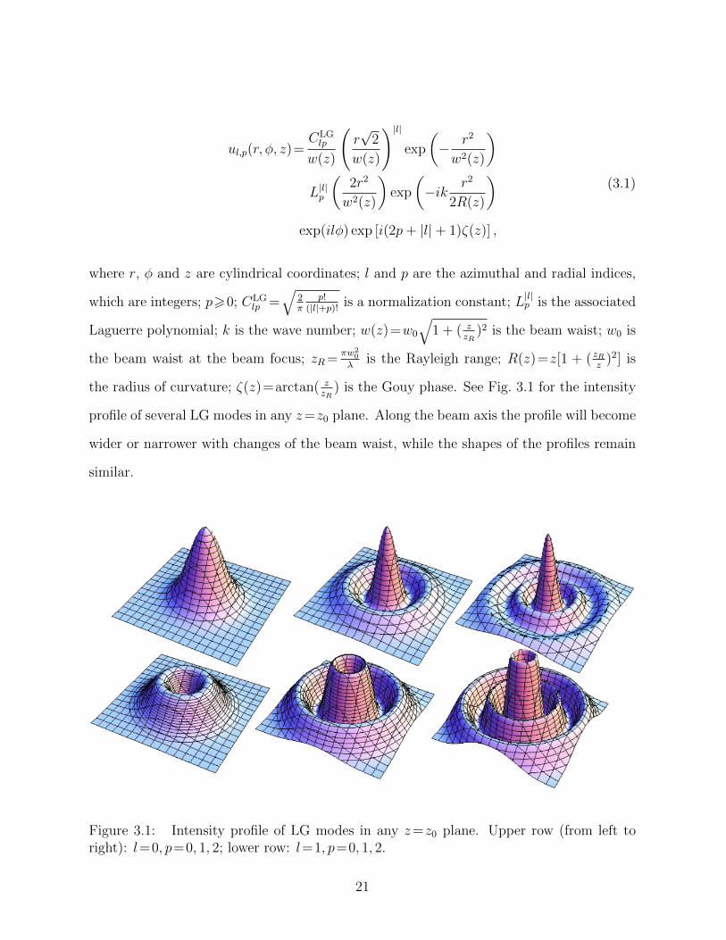
) is the Gouy phase. See Fig. 3.1 for the intensity
profile of several LG modes in any z=z0 plane. Along the beam axis the profile will become
wider or narrower with changes of the beam waist, while the shapes of the profiles remain
similar.
Figure 3.1: Intensity profile of LG modes in any z=z0 plane. Upper row (from left toright): l=0, p=0, 1, 2; lower row: l=1, p=0, 1, 2.
21

In free space the LG modes propagate independently without interacting with each
other; they obey the following orthonormality conditions,
∫z=z0
ul,pu∗l′,p′rdrdφ=δll′δpp′ . (3.2)
Notice, the orthogonality condition only holds if the integration area on the left hand side
of Eq. (3.2) is the entire z=z0 plane.
Now, let us consider putting a spatial mask (such as a circular iris) in the z=z0 plane,
shown in Fig. 3.2. The iris blocks or absorbs the field at the rim and allows the field at
the opening to pass through. For LG modes, the part of them allowed to pass through the
opening of iris no longer obeys orthogonality. Physically this means different LG modes will
interact at the plane where the iris is placed. The interaction of modes can be described
by the following expression,
∫S
ul,pu∗l′,p′rdrdφ=Bl,l′,p,p′ , (3.3)
where S is the surface through which the spatial mask permits the light to pass. For a
circular iris with radius a, centered on the beam axis, placed in z=z0 plane, S={r<a; z=
z0}.
Since in free space LG modes form an orthonormal basis, both the input signal (at
z=z0−) and the output signal (at z=z0
+) can be expressed as linear combinations of LG
modes, which both satisfy paraxial approximation. Further, in free space on both sides of
the iris [z∈(−∞, z0)∪ (z0,+∞)], the orthogonality of LG modes holds, and the iris (z=z0)
is the only location where orthogonality breaks. Therefore the coefficient of each LG mode
will change only when the signal goes through the iris. We express this interaction using
the following set of equations: the input beam takes the form,
uinput(r, φ, z)=∑l,p
Al,p × ul,p(r, φ, z); (z<z0), (3.4)
22

Figure 3.2: The iris, with a circular opening of radius a, is applied along the beam axis.The red curve is the Gaussian beam width w(z) as a function of z. The iris is located atthe plane z=z0. The center of iris is on the z axis. The amplitude will be truncated to zeroat the rim of the iris, while in the opening of the iris the amplitude will be unchanged. Asa result the orthogonality between LG modes will be broken, and the modes will interactat the iris plane.
23

where Al,p is the coefficient of each LG mode. At the iris the beam is partially absorbed
and thus we have,
uiris(r, φ, z0)=
∑l,pAl,p × ul,p(r, φ, z0); (r<a, z=z0)
0; (r≥a, z=z0),
(3.5)
satisfying the boundary condition at the iris, giving the output signal,
uiris(r, φ, z0)=uoutput(r, φ, z0+), (3.6)
which finally leads to,
uoutput(r, φ, z)=∑l,p
Al,p∑l′,p′
Bl,l′,p,p′ × ul′,p′(r, φ, z); (z>z0). (3.7)
The quantity Bl,l′,p,p′ , first introduced in Eq. (3.3), is the transformation coefficient between
LG mode l, p and l′, p′. Solving Eqs.(3.4, 3.5, 3.6, 3.7), we get,
Bl,l′,p,p′=Cl,l′,p,p′ × exp[i(2p− 2p′ + |l| − |l′|)ζ(z0)]. (3.8)
Here we express the complex quantity Bl,l′,p,p′ in polar form, as it more clearly shows the
role of ζ(z0), which is the Gouy phase at the iris position. The factor Cl,l′,p,p′ is real
in the circular iris situation, since the cylindrical symmetry prevents interaction between
azimuthal indexes:
Cl,l′,p,p′=δll′ ×2a2/w2(z0)∫
0
exp (−x)L|l|p (x)L|l′|p′ (x)dx. (3.9)
24

It is due to the limitation in the radial direction, introduced by the iris, that different
p modes will interact. But due to the cylindrical symmetry of the iris, different l modes
will remain orthogonal. Therefore, if instead of a circular iris, other types of spatial masks
(that do not have cylindrical symmetry) are used, orthogonality amongst l modes will
be broken, and different l modes will interact with each other. The interactions, which
are characterized by the transformation coefficient, will be determined by the shape and
position of the spatial mask. For the remainder of this paper, we consider only an iris
spatial mask because of its simplicity. However our theory applies to all spatial masks,
and the transformation coefficients can be calculated in a similar manner. To calculate
transformation coefficients for an arbitrary spatial mask, we can still make use of the more
general Eq. (3.3) instead of Eqs. (3.8, 3.9), which are specifically suitable for circular iris
mask centered on beam axis.
3.3 Quantization of Gaussian Modes
In free space, due to orthogonality, each mode of the Gaussian beam propagates without
interacting with another. Therefore, the quantum state of each mode will evolve indepen-
dently. A pure quantum state without mode entanglement is a product state of every
quantum state in every Gaussian mode:
|ψ〉=l=+∞,p=+∞∏l=−∞,p=0
|ψl,p〉 . (3.10)
The separable state forms a building block for more complicated states. A general
pure state, with or without mode entanglement, can be expressed as a linear combination
of separable states in the form of Eq. (3.10). Further, a mixed state can be expressed as
probabilistic sum of pure states.
When a spatial mask such as an iris is applied to the Gaussian beam, the quantum
states of different modes will interact. The interaction can be described as a transforma-
tion of annihilation or creation operators of input modes into operators of output modes.
This transformation should be unitary, which preserves the commutation relations of the
25

annihilation or creation operators. However, one problem needs to be solved. Generally,
spatial masks (or other optical devices) are lossy. For example, an iris will absorb part of
the input signal at the rim. A widely accepted procedure [42] to deal with loss in quantum
optics is to introduce “absorption modes” which we denote as: A1, A2, .... To be clear, we
call the original Gaussian modes “signal modes”, since they are the ones that may contain
information, such as squeezing levels and squeezing angles. We denote the signal modes
with simply l and p numbers. Further, we denote with a prime symbol on the operators
of output modes to differentiate them from the input modes. The transformation, caused
by the iris, from the operators of input modes into those of output modes, is illustrated in
Fig. 3.3.
Before we continue, let us explain a bit more about the absorption modes. They serve
three purposes. The first purpose is that they describe the absorption (loss) of the field.
Since the states in output-signal modes are described by tracing the entire output density
matrix over the absorption modes, the total energy of the signal is generally decreased.
The second purpose is that they help to keep the transformation unitary by expanding
the dimension of the transformation matrix [43]. The reader might remember a similar
principle applies when modeling loss with a simple beam splitter; we must consider a second
input even if only the first input is used [42]. The third purpose of the absorption modes
is that they naturally introduce the vacuum fluctuations and accommodate the common
observation that fluctuations usually occur with losses.
The model works in the following way. The quantum states of the input signal modes
can be arbitrary, but quantum states in the input-absorption modes are vacuum. A unitary
transformation transforms the operators of input-signal or absorption modes into opera-
tors of output-signal or absorption modes; illustrated in Fig. 3.3. Once we obtain output
operators in terms of input operators we can then calculate the quantum states in the
output-signal or absorption modes. The quantum state in all output modes then needs
to be traced over the output absorption modes, and finally we obtain the reduced density
26
matrix that describes the quantum state in the output-signal modes, which generally is a
mixed state, even if the input state is a pure state. Later we will give a few examples for
a variety of input states.
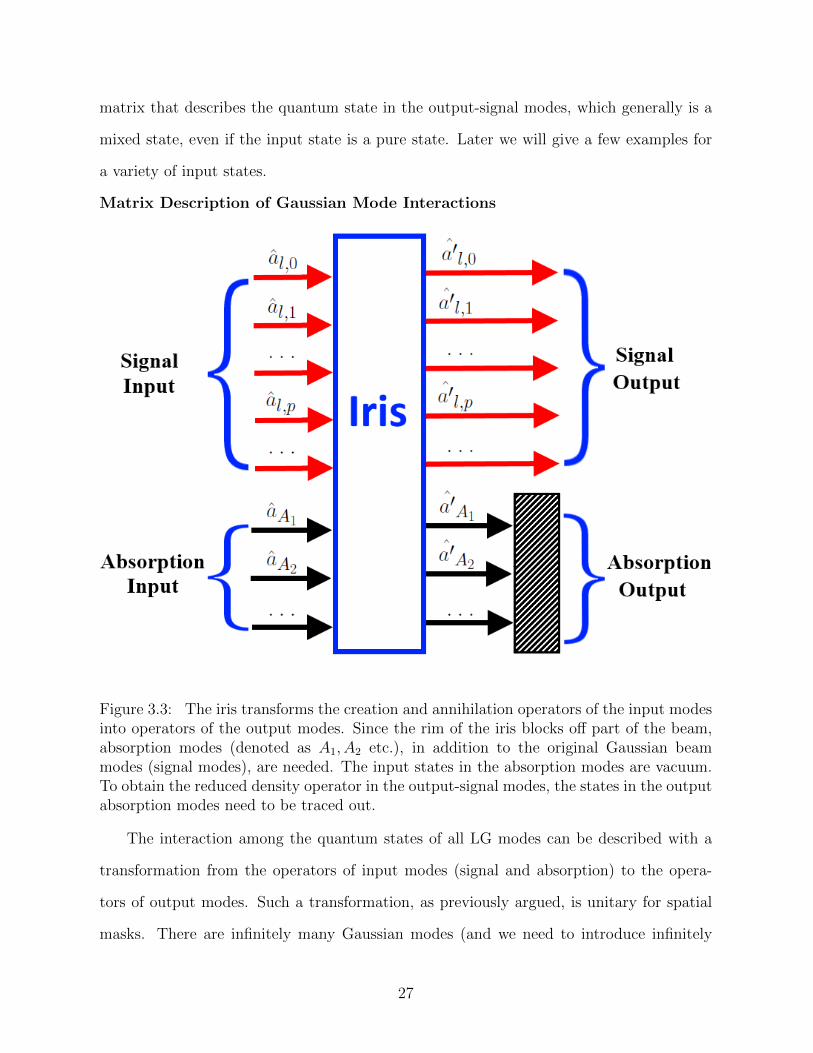
Matrix Description of Gaussian Mode Interactions
Figure 3.3: The iris transforms the creation and annihilation operators of the input modesinto operators of the output modes. Since the rim of the iris blocks off part of the beam,absorption modes (denoted as A1, A2 etc.), in addition to the original Gaussian beammodes (signal modes), are needed. The input states in the absorption modes are vacuum.To obtain the reduced density operator in the output-signal modes, the states in the outputabsorption modes need to be traced out.
The interaction among the quantum states of all LG modes can be described with a
transformation from the operators of input modes (signal and absorption) to the opera-
tors of output modes. Such a transformation, as previously argued, is unitary for spatial
masks. There are infinitely many Gaussian modes (and we need to introduce infinitely
27

many absorption modes as well). Therefore, in the most general case, quantum states or
operators in infinitely many input modes are transformed into quantum state or operators
in infinitely many output modes.
Although this might seem complicated, sometimes the transformation can be greatly
simplified when the spatial mask has some kind of symmetry. For example, as we previously
pointed out, an iris has cylindrical symmetry and LG modes with different l’s do not interact
(due to the Kronecker delta in Eq. (3.9), which enforces angular momentum conservation).
Therefore, for a circular iris, we need only to examine the transformation of LG modes with
the same l but different p’s. To that end, we introduce the column vector of annihilation
operators for input LG mode (l, p=0), (l, p=1), (l, p=2) etc. as well as operators for input-
absorption modes A1, A2, A3 etc,
(al)=
(al,0 al,1 · · · aA1 aA2 · · ·
)T. (3.11)
The creation operators are similarly,
(al†)=
(a†l,0 a†l,1 · · · a†A1
a†A2· · ·)T
, (3.12)
and the output modes follow, but they are marked with prime
(a′l)=
(a′l,0 a′l,1 · · · a′A1 a′A2 · · ·
)T, (3.13)
(a′l†)=
(a′†l,0 a′
†l,1 · · · a′
†A1
a′†A2· · ·)T
. (3.14)
We also define the unitary transformation matrix Jl, which determines the interaction
among LG modes with same l, but different values of p.
28

Jl=
Jl;0,0 Jl;0,1 . . . Jl;0,A1 Jl;0,A2 . . .
Jl;1,0 Jl;1,1 . . . Jl;1,A1 Jl;1,A2 . . .
. . . . . . . . . . . . . . . . . . . . . . . . . . . . . . . . . . . . . . . .
Jl;A1,0 Jl;A1,1 . . . Jl;A1,A1 Jl;A1,A2 . . .
Jl;A2,0 Jl;A2,1 . . . Jl;A2,A1 Jl;A2,A2 . . .
. . . . . . . . . . . . . . . . . . . . . . . . . . . . . . . . . . . . . . . .
. (3.15)
(a′)=J × (a)
The transformation of input and output operators can be expressed in the following
compact form
(al′)=Jl × (al), (3.16)
(a′l†)=J ∗l × (al
†). (3.17)
J ∗l stands for the conjugate (without transpose) of Jl. The signal-signal elements (Jl;0,0, Jl;1,0, Jl;0,1,
etc.) in the matrix Jl determine the transformation between input and output-signal
modes. Here we make use of Bohr’s correspondence principle. For large amplitude coher-
ent states in the input signal modes, the transformation between input and output-signal
modes should agree with the classical result in Eq. (3.7), giving,
Jl;p1,p2 =Bl,l,p1,p2 , (3.18)
which can be calculated using Eqs. (3.8, 3.9). As for the other (signal-absorption and
absorption-absorption) elements in Jl, we can make use of Jl being unitary. This gives
JlJ †l =I, which will give equations describing the relations among the Jl elements. Of
course, signal-absorption and absorption-absorption elements might not be completely
fixed, and there might be a certain freedom of choice. In fact, they may not need to
be calculated at all. We find that, in the calculations we have done so far, we can always
29

eliminate signal-absorption and absorption-absorption elements using the condition that
Jl is unitary.
Indeed, if one aims for completeness, one should consider infinitely many LG modes.
However, we do not usually have that luxury, since the dimension of the transformation
matrix grows with the number of modes, and we are forced to consider a limited number of
modes. Intuitively, the more modes we consider, the better. But the effect of higher-order
modes often diminishes at a very fast rate. As we show in the next section, we are able to
explain our experimental data, even if we consider only two input signal modes and two
absorption modes.
For a spatial mask with arbitrary shape, we cannot exploit the cylindrical symmetry as
we did with the iris. However, we can still introduce similar column vector of operators as
before, but we now will need to include various l modes together instead of only considering
one l mode at a time. We can achieve this by defining a concatenation of column vectors
of operators, such as (a)=
((al=0)T (al=1)T (al=−1)T · · ·
)T, in which every element is
defined in Eq. (3.11). The transformation matrix J between input to output modes needs
to be expanded in similar fashion in order to accommodate different l modes; and the
integration area of Eq. (3.3) needs to be changed as well. Then we can finally arrive at the
relation similar to Eq. (3.16): (a′)=J (a).
Unlike the iris, a spatial mask without cylindrical symmetry introduces interaction
between orbital angular momentum modes, which can be very useful. However the purpose
of this work is not to explore novel designs of optical devices, but to setup a general method
for analyzing a range of problems. For now, the simple iris is enough to serve such a purpose,
but we stress that our method can also accommodate optical devices without cylindrical
symmetry.
30

3.4 Additional Examples of the Use of the Theory
3.4.1 Example 1: Squeezed-vacuum Input States and the Wigner Function
Description
Let us consider the following model. In the two signal LG modes of (l=0, p=0)
and (l=0, p=1), we input two squeezed-vacuum quantum states, which are defined as
S(ξ0) |0〉l=0,p=0 and S(ξ1) |0〉l=0,p=1, respectively, while in every other LG mode we input
vaccum states. The squeezing operators are defined as S(ξp)=exp[12(ξ∗p a
20,p − ξpa
†20,p)], with
p=0, 1. The squeezing parameters are ξ0 =r0 exp(iθ0) and ξ1 =r1 exp(iθ1).
Let us further consider a classical field with large amplitude, in the (l=0, p=0) LG
mode, acting as a local oscillator (LO) for homodyne detection. The signal and local
oscillator co-propagate with each other along the beam axis, but they are in perpendicular
polarizations.
Now we insert a circular iris in the neighborhood of the beam focus point and centered
on the beam axis, shown in Fig. 3.4. According to our theory, both the signal and LO are
influenced by the iris in the way described in previous sections. Introduced by the iris, the
interaction among LG modes mainly happens between (l=0, p=0) and (l=0, p=1) modes.
Therefore we can simplify the calculation by considering only two input- (or output-) signal
modes and two absorption modes, instead of taking into account infinitely many input (or
output) modes. The diagram of this model is shown in Fig. 3.5. We then move the iris along
the beam axis, and numerically simulate the minimum noise measured in the homodyne
detection vs. the iris position, shown in Fig. 3.6. We can also use different-sized irises,
which are represented by different curves. The experimental counterpart of this simulation
is investigated in Ref. [2].
In order to gain a clearer and more intuitive view, we now examine our model in the
Wigner representation. It is essential to understand how the iris transforms the input
Wigner function into the output Wigner function. We first use Eq. (3.16) and (3.17) to
31

Figure 3.4: Model setup. The single-mode squeezed vacuum states are in (l=0, p=0) and(l=0, p=1) LG modes, while the local oscillator is in (l=0, p=0) LG mode. The squeezedvacuum and the local oscillator co-propagate but are in perpendicular polarizations. Thespatial mask consists of a one-to-one telescope and an iris between the lenses. We movethe iris along the beam axis and find the minimum noise in each case.
32

Figure 3.5: Instead of taking into account of infinitely many input or output modes, weconsider only two input- (or output-) signal modes and two absorption modes, because theinput states in the (l=0, p=0) and (l=0, p=1) LG modes are the only ones that are non-vacuum, and the interaction between the two modes far exceeds the interaction betweenother LG modes.
Figure 3.6: Minimum noise in homodyne detection vs the iris position. Different sizedirises are represented by different curves, and they are denoted by the percentage of peaktransmission through the iris relative to full beam transmission, as well as the iris radius(scaled by w0). We only apply one iris at a time. The input states in the (l=0, p=0) and(l=0, p=1) LG modes are squeezed states with different squeezing parameters: r0 =0.3,θ0 =0, r1 =0.4, θ1 =0.325π.
33

calculate the transformation between input and output modes operators, and obtain the
transformation of quadratures,
ql,0
ql,1
qA1
qA2
=Re(Jl)
q′l,0
q′l,1
q′A1
q′A2
− Im(Jl)
p′l,0
p′l,1
p′A1
p′A2
, (3.19)
pl,0
pl,1
pA1
pA2
=Re(Jl)
p′l,0
p′l,1
p′A1
p′A2
+ Im(Jl)
q′l,0
q′l,1
q′A1
q′A2
. (3.20)
Then we substitute the input quadratures with output quadratures, thus completing the
transformation of input Wigner function to output Wigner function.
W (q0,0, p0,0, q0,1, p0,1, qA1, pA1, qA2, pA2)
Eq. (3.19)(3.20)−−−−−−−−−→W (q′0,0, p′0,0, q
′0,1, p
′0,1, q
′A1, p
′A1, q
′A2, p
′A2)
(3.21)
To make our example more general, we now replace squeezed vacuum with displaced
squeezed states as input states: D(α0)S(ξ0) |0〉l=0,p=0 and D(α1)S(ξ1) |0〉l=0,p=1 in (l=0, p=
0) and (l=0, p=1) LG modes. The displacement operator for l=0, p=1, 2 mode is defined
as D(αp)=exp(αpa†0,p − α∗pa0,p). The Wigner functions of the quantum states in the two
input-signal modes are:
34

W (qm, pm)
=1
πexp{−e−2rm [(pm − pm) cos (θm/2)
− (qm − qm) sin (θm/2)]2}
× exp{−e2rm [(qm − qm) cos (θm/2)
+ (pm − pm) sin (θm/2)]2},
(3.22)
where qm, pm are the quadratures of mode (l=0, p=m) and m=0, 1, and qm= 1√2(αm +
α∗m), pm= i√2(−αm + α∗m), ξm=rm exp(iθm). For absorption modes the input states are
vacuum, whose Wigner functions are:
W (qn, pn)=1
πexp(−q2
n − p2n), (3.23)
where n=A1, A2. Since the total input state is a product state of states in each of the four
input modes, the total input Wigner function is:
W (q0,0, p0,0, q0,1, p0,1, qA1, pA1, qA2, pA2)
=W (q0,0, p0,0)W (q0,1, p0,1)W (qA1, pA1)W (qA2, pA2).
(3.24)
We keep the input state fixed and change the position of the iris along beam axis. The
change in iris position changes the matrix elements of Jl=0 in Eqs. (3.19, 3.20), which in turn
changes the output states in three ways: (a) the squeezing and anti-squeezing level changes,
(b) the squeezing angle changes, and (c) the state displacement (from vacuum) changes.
The Wigner functions of the input state (as well as output states) of different iris positions
are plotted in Fig. 3.7. It is also worth noting that, despite the input-signal states in this
35

example being pure states (displaced squeezed-vacuum states in each of the two LG modes),
the output-signal states are generally mixed states. This is mainly because we obtain the
reduced density operator for the signal modes by tracing the total density operator over the
absorption modes. As a result, the output states are no longer pure minimum uncertainty
states. To verify this we can simulate the squeezing and anti-squeezing noise in each output
LG mode vs. the iris position; shown in Fig. 3.8. For a minimum-uncertainty squeezed
state, the squeezing and anti-squeezing noise should add up to 0 dB, which means the
squeezing and anti-squeezing noise curve for of the same mode should be symmetric about
the horizontal axis in Fig. 3.8. This is obviously not the case, which verifies that the output-
signal state is not a minimum uncertainty state in either LG mode. The noise measurement
in Fig. 3.8 is achievable in an experiment. For instance, we can make use of homodyne
detection and adjust the local oscillator to be in one particular single output LG mode with
a spatial light modulator. Notice the noise measurement described in Fig. 3.6 is different.
In that previous case, the local oscillator co-propagates with the signal and both of them
are influenced by the iris; after the iris the local oscillator consists of multiple LG modes
instead of a single mode. We would like to emphasize that every example is applicable for
any suitable detection scheme without being limited to homodyne detection. For example
in section C. below we predict a Hong-Ou-Mandel-like effect for which coincident detection
is required and not homodyne.
Now we will show a rather surprising result, namely that the spatial mask behaves
like a multi-port beam splitter with loss. To elaborate this point, let us consider the
following situation. In the case of the input states of a beam splitter being two single-mode
squeezed-vacuum states with identical squeezing parameters, it is well known [42] that the
output state will be a two-mode squeezed state, if the beam splitter is perfectly 50:50.
Now, let us use an iris instead of a beam splitter. We put identical single-mode squeezed-
vacuum states in both input LG modes (l=0, p=0) and (l=0, p=1). After the states go
through the iris, we then calculate the probability of detecting n0,0 and n0,1 photons in
36

Figure 3.7: First column from the left: Input displaced-squeezed state Wigner func-tion. Top row: LG mode l=0, p=0; bottom row: LG mode l=0, p=1. The inputstates are displaced squeezed-vacuum with displacement parameters α0 =1.5 exp(πi) andα1 =2 exp(1.5πi), and squeezing parameters r0 =0.5, θ0 =0.25π, r1 =0.8, θ1 =0.75π. Sec-ond column: Output quantum state Wigner function when iris is located at z=−zR (oneRayleigh range before the focus). Third column: Output quantum state Wigner functionwhen iris is located at z=0. Fourth column: Output quantum state Wigner function wheniris is located at z=zR. Iris radius is w0. This provides evidence that moving the iris isrotating the squeezing angles via the Gouy phase. Note that the input-signal states shownin this graph are pure states, while the output-signal states in both LG modes are mixedstates.
37

Figure 3.8: Noise of squeezing and anti-squeezing of l=0, p=0 and l=0, p=1 LG modesvs. iris position, which is shown in the units of Rayleigh range. The parameters of theinput states and iris size are the same with the parameters described in the caption ofFig. 3.7. Notice that the squeezing and anti-squeezing noise curve for of the same modeare not symmetrical about the horizontal axis (0dB noise level line) for displaced-squeezedinput states. This is because the quantum state in each LG mode is no longer a minimumuncertainty state.
38

(a) (b)
Figure 3.9: The joint probability Pn0,0,n0,1 vs. n0,0 vs. n0,1 in (a) input LG (l=0, p=0)and (l=0, p=1) modes, and (b) the same two LG modes in the output. The squeezingparameters of the squeezed-vacuum states in the input modes are r0 =r1 =1, θ0 =θ1 =0.The iris is placed at z=0 and the radius of the iris is 0.8339w0. Note that the non-zeroprobability for the one-one block provides evidence that the iris has converted the twoseparable squeezed-vacuum inputs into an entangled two-mode squeezed-vacuum output.
the output LG modes (l=0, p=0) and (l=0, p=1), shown in Fig. 3.9b. For comparison,
we show the probability in the input modes as well in Fig. 3.9a. We can see in the input
modes, since the quantum state is a product state of two single-mode squeezed-vacuum,
the probability is non-zero only at even n0,0 and n0,1. If the state in the output modes is
indeed a two-modes squeezed state, the probability is non-zero only at n0,0 =n0,1, namely
n0,0 =n0,1 =0, n0,0 =n0,1 =1, n0,0 =n0,1 =2, etc. However, one important visible change from
the two single-mode squeezed-vacuum states to a two-mode squeezed-vacuum state is that
the two-mode joint probability Pn0,0=1,n0,1=1 is zero in the former and non-zero in the latter
[43]. This is indeed the case, as we can see in Fig. 3.9, which verifies our conjecture–a hole
is like a beam splitter. We can also see that the Fig. 3.9b does not give a ideal two-mode
squeezed state, this is because the iris is imbalanced (the different modes have different
radial profiles) and lossy, as opposed to a perfect 50 :50 beam splitter.
We can see how Pn0,0=1,n0,1=1 and Pn0,0=3,n0,1=3 would change with the iris size in
Fig. (3.10a, 3.10b). Both of them reduce to zero when iris is completely closed, where
the output state is reduced to vacuum. Notice Pn0,0=1,n0,1=1 and Pn0,0=3,n0,1=3 also reduce
to zero in case of large iris size, where the output state is reduced to the same as the in-
put the state (a product state of two single-mode squeezed-vacuum states). The non-zero
39

Pn0,0=1,n0,1=1 and Pn0,0=3,n0,1=3 are what give the distinct feature of two-mode squeezing,
which is most visible when the iris is neither too large nor too small, which is where the
maximal interaction between LG modes (l=0, p=0) and (l=0, p=1) takes place.
We can also investigate the covariance of the photon numbers in the two input modes
or the two output modes, which is defined as [43],
Cov(n0,0, n0,1)=〈n0,0n0,1〉 − 〈n0,0〉 〈n0,1〉 . (3.25)
For single-mode squeezed-vacuum states in the two input modes, the covariance is
obviously zero since the state in each mode is independent. However, in the output modes of
the iris, we should see generally non-zero covariance due to the beam-splitter-like interaction
introduced by the iris, if indeed that interaction produces entangled two-mode squeezed
vacuum. In this case, where we consider only LG (l=0, p=0) and (l=0, p=1) modes and
two other absorption modes, the output covariance is
Cov(n0,0, n0,1)=C20,0,0,0C
20,0,0,1 sinh2 r0 cosh2 r0
+ C20,0,0,1C
20,0,1,1 sinh2 r1 cosh2 r1
+ 2C0,0,0,0C0,0,0,1C20,0,0,1 sinh r0 sinh r1
× (sinh r0 sinh r1 + cosh r0 cosh r1 cos[4ζ(z0) + θ0 − θ1]),
(3.26)
where z0 is the iris position and Cl,l′,p,p′ ’s can be calculated using Eq. (3.9). We can see
in Eq. (3.26) the joint effect on the covariance by the Gouy phase ζ(z0) and the squeezing
angles θ0 and θ1 of the two input squeezed states. If θ0 and θ1 are different to begin with,
we can counteract such difference by altering the iris position z0 to change the Gouy phase.
We can see how the covariance would change with iris radius in Fig. 3.11.
To sum up, when applied to a Gaussian beam, the spatial mask behaves very much like
a multi-port beam splitter with loss. If the input quantum states are displaced squeezed
states, the spatial mask alters the displacement, which is a classical phenomenon; the spatial
40
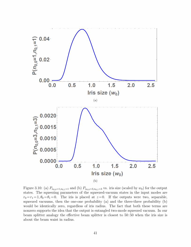
(a)
(b)
Figure 3.10: (a) Pn0,0=1,n0,1=1 and (b) Pn0,0=3,n0,1=3 vs. iris size (scaled by w0) for the outputstates. The squeezing parameters of the squeezed-vacuum states in the input modes arer0 =r1 =1, θ0 =θ1 =0. The iris is placed at z=0. If the outputs were two, separable,squeezed vacuums, then the one-one probability (a) and the three-three probability (b)would be identically zero, regardless of iris radius. The fact that both these terms arenonzero supports the idea that the output is entangled two-mode squeezed vacuum. In ourbeam splitter analogy the effective beam splitter is closest to 50:50 when the iris size isabout the beam waist in radius.
41

Figure 3.11: Covariance of output LG modes vs. iris radius. The squeezing parameters ofthe two, separable, squeezed-vacuum states in the input modes are r0 =r1 =1, θ0 =θ1 =0.The iris is placed at z=0. We can see the covariance between the two output modes ispeaked at the radius of the iris being 0.8339w0, which is the iris radius we use in Fig. 3.9b.Also the reader might be interested to know that so long as the squeezing parameters in LG(l=0, p=0) and (l=0, p=1) modes are the same, the covariance always peaks if the iris isplaced at z=0 with a radius of 0.8339w0. In our beam splitter analogy, if the outputs wereagain two, separable, single-mode squeezed vacuums, the covariance would be identicallyzero for all iris radii, which is clearly not the case. If the iris acted like a perfect 50 :50beam splitter, the covariance would be 1
4sinh2(2r)≈3.29 [43]. However due to loss and
mode mismatch it peaks here at 0.65. Again it peaks when iris radius is about beam waistwhere LG (l=0, p=0) and (l=0, p=1) mode overlap is maximal.
42

Figure 3.12: As in the previous example, we consider two signal modes: LG mode (l=0, p=0) and (l=0, p=1), along with two absorption modes A1, A2. The input state is aproduct state of single photon in (l=0, p=0) mode and vacuum in other modes: |1〉l=0,p=0⊗|0〉l=0,p=1⊗|0〉A1
⊗|0〉A2. After the two output absorption modes are traced over, the reduced
density matrix of the two output-signal modes, ρrel=0,p=0,1, is given in Eq. (3.36). We show
in the Fig. 3.13 that the output state has number-path entanglement, created by the iris.
mask also alters the squeezing levels and angles, which is a non-classical phenomenon. Note
that even though the input squeezed states are pure, minimum uncertainty states, the
output states are generally mixed states with Wigner functions similar to displaced squeezed
thermal states. The spatial mask also behaves similarly to a beam-splitter transforming a
product state of two single-mode squeezed vacuums into, to an extent, an entangled two-
mode squeezed state. Although this transformation is not perfect, since the spatial mask is
lossy and imbalanced compared to a 50:50 beam-splitter, there can be no doubt that even
a device as simple as an iris should be treated quantum mechanically like a beam splitter.
3.4.2 Example 2: Single Photon in One Input State and Generation of Number-
path Entanglement
In this example we input a single-photon state in signal mode (l=0, p=0) and a vacuum
state in signal mode (l=0, p=1) as well as absorption modes A1, A2. (The input states
43

for absorption modes are always vacuum.) Therefore the total input state in four modes
is |1〉l=0,p=0 ⊗ |0〉l=0,p=1 ⊗ |0〉A1⊗ |0〉A2
, shown in Fig. 3.12. For the vacuum state, the
corresponding Wigner function is again,
WN=0(q, p)=1
πexp[−(q2 + p2)], (3.27)
where N is the photon number. For the single photon state, the corresponding Wigner
function is [42]
WN=1(q, p)=−1
πexp[−(q2 + p2)]L1(2q2 + 2p2), (3.28)
where LN is the N th order Laguerre polynomial. The overall Wigner function (for LG
signal modes (l=0, p=0) and (l=0, p=1) and absorption modes A1 and A2) is therefore,
W (q0,0, p0,0, q0,1, p0,1, qA1, pA1, qA2, pA2)
=WN=0(q0,0, p0,0)WN=1(q0,1, p0,1)
×WN=0(qA1, pA1)WN=0(qA2, pA2).
(3.29)
Using the same method in the last example we calculate the Wigner function of output
modes. We then can calculate the Wigner function for either output mode, for example,
LG mode (l=0, p=0), by tracing over the other modes:
Wl=0,p=0(q′0,0, p′0,0)
=
∫W (q′0,0, p
′0,0, q
′0,1, p
′0,1, q
′A1, p
′A1, q
′A2, p
′A2)
× dq′0,1dp′0,1dq′A1dp′A1dq′A2dp′A2
=(1− |Jl=0;0,0|2)WN=0(q′0,0, p′0,0)
+ |Jl=0;0,0|2WN=1(q′0,0, p′0,0).
(3.30)
44

Therefore, in the output-signal LG mode (l=0, p=0), the reduced density operator is,
ρrel=0,p=0 =(1− |Jl=0;0,0|2) |0〉 〈0|+ |Jl=0;0,0|2 |1〉 〈1| . (3.31)
With a similar calculation, we find in the output-signal LG mode (l=0, p=1), the
reduced density operator is,
ρrel=0,p=1 =(1− |Jl=0;0,1|2) |0〉 〈0|+ |Jl=0;0,1|2 |1〉 〈1| . (3.32)
From Eqs. (3.31, 3.32) we can immediately see that if we fire a single photon in the (l=
0, p=0) mode and vacuum in the (l=0, p=1) mode, that the photon will have a |Jl=0;0,0|2
chance of staying in the (l=0, p=0) mode at the output and a |Jl=0;0,1|2 chance of switching
to the (l=0, p=1) output mode. Similarly, it is not difficult to find that if we fire a single
photon in the (l=0, p=1) mode and vacuum in the (l=0, p=0) mode, that photon will
have a |Jl=0;1,1|2 chance of staying in the (l=0, p=1) mode at the output and a |Jl=0;1,0|2|=
Jl=0;0,1|2 chance of switching to the (l=0, p=0) output mode. We will take another look
at this result in example 3.
However, only looking at each output mode separately does not give us the insight
of correlation between modes. To achieve that we need to consider the reduced density
operator for both the output-signal LG modes (l=0, p=0) and (l=0, p=1), this state
is generally mixed, and perhaps more interestingly, contains number-path entanglement,
which again is also created when a single photon strikes an ordinary 50:50 beam splitter.
To see this, let us examine the Wigner function in two output-signal modes:
45

Wl=0,p=0,1(q′0,0, p′0,0, q
′0,1, p
′0,1)
=1
π2exp[−(q′20,0 + q′20,0 + q′20,1 + q′20,1)]
×[(1− |Jl=0;0,0|2 − |Jl=0;0,1|2)
+ |Jl=0;0,0|2L1(2q′20,0 + 2q′20,0)
+ |Jl=0;0,1|2L1(2q′20,1 + 2q′20,1)
+ 2Jl=0;0,0J∗l=0;0,1(p′0,0 − iq′0,0)(p′0,1 + ip′0,1)
+ 2J∗l=0;0,0Jl=0;0,1(p′0,0 + iq′0,0)(p′0,1 − ip′0,1)].
(3.33)
The quantum state corresponding to the Wigner Function given in Eq. (3.33) is a mixed
state of (a) the vacuum state,
|φ1〉= |0〉l=0,p=0 ⊗ |0〉l=0,p=1 ,(3.34)
with probability of 1− |Jl=0;0,0|2 − |Jl=0;0,1|2, and (b) an entangled state of the form,
|φ2〉=J∗l=0;0,1√
(|Jl=0;0,0|2 + |Jl=0;0,1|2)|0〉l=0,p=0 ⊗ |1〉l=0,p=1
+J∗l=0;0,0√
(|Jl=0;0,0|2 + |Jl=0;0,1|2)|1〉l=0,p=0 ⊗ |0〉l=0,p=1 ,
(3.35)
with probability of |Jl=0;0,0|2 + |Jl=0;0,1|2. Therefore the reduced density matrix for the
output-signal LG mode (l=0, p=0) and (l=0, p=1) is,
ρrel=0,p=0,1 =(1− |Jl=0;0,0|2 − |Jl=0;0,1|2) |φ1〉 〈φ1|
+(|Jl=0;0,0|2 + |Jl=0;0,1|2) |φ2〉 〈φ2| .(3.36)
46

One can verify this result by calculating the Wigner function of ρrel=0,p=0,1 and compar-
ing it with Eq. (3.33). Other works have also been done to demonstrate the entanglement
generation using spatial masks [44, 45, 46]. One can examine the violation of the Clauser-
Horne (CH) Bell inequality [47, 48] of the entangled state |φ2〉. The more CH combination
drops below −1, the easier the violation can be observed [49]. Therefore by plotting the
minimized Clauser-Horne combination vs. iris position, shown in Fig. 3.13, we can quanti-
tatively determine the extent of the entanglement, which is generated by the iris, that can
be observed.
Figure 3.13: Minimized Clauser-Horne combination vs iris position for different sizedirises. The CH combination is minimized in phase space. Notice that the minimized CHcombination is below −1, proving the Bell inequality is violated. The more CH combinationdrops below −1, the easier the violation can be observed. In our beam splitter analogyit is well know [43] that a single photon incident on a 50:50 beam splitter produces theentangled state, 1√
2(|1〉 |0〉+ i |0〉 |1〉).
47

3.4.3 Example 3: Single Photon in Each of Two Input States and a Hong-Ou-
Mandel-like Effect
It is well known that when two identical photons are inputted into two separate modes
of a beam splitter, photon bunching occurs. We show here the iris produces a similar effect
on two LG modes. Now let us input a single photon state in mode (l=0, p=0) and another
single photon state in mode (l=0, p=1). Photon detectors are used to detect the photon
numbers in the two output-signal LG (l=0, p=0) and (l=0, p=1) modes, then the photon
detector count signals are fed into a correlator. The setup diagram is shown in Fig. 3.14.
We then repeat this experiment multiple times so that we can measure the probability of
detecting a single photon in each of the output-signal modes, which is refereed to as the
coincidence probability. The goal is to produce a spatial mask version of Hong-Ou-Mandel
(HOM) effect [50]. Previous works have already been done to demonstrate the HOM effect
in multiple spatial modes experiments [51, 52, 53].
Let us first examine the case where, apart from being in different modes, the single
photon state in mode (l=0, p=0) and the single photon state in mode (l=0, p=1) are
completely distinguishable. This distinguishability can be caused by many reasons, such as
the two photons having orthogonal polarizations or large frequency difference or large time
delay when they are fired. In this case when the two photons are completely distinguishable,
the two photons will not interfere and the case can be viewed simply as two independent
experiments combined: (a) input one photon in mode (l=0, p=0) and vacuum in other
modes; (b) input one photon in mode (l=0, p=1) and vacuum in other modes. Therefore we
can simply use the analysis in example 2, and the coincidence probability is the probability
that both photon staying in the same modes at the output plus the probability that both
photons switching to the other modes, which is J20;0,0∗J2
0;1,1 + |J0;1,0|2∗|J0;0,1|2 =J20;0,0J
20;1,1 +
|J0;1,0|4.
48

Figure 3.14: Single-photon state in both of the two input-signal modes: LG mode (l=0, p=0) and (l=0, p=1), and vacuum state in the two input-absorption modes A1, A2.Therefore the total input state of the four modes is: |1〉l=0,p=0 ⊗ |1〉l=0,p=1 ⊗ |0〉A1
⊗ |0〉A2.
The coincidence probability of the two output-signal modes is given by the probability ofthe photon detectors receiving one photon each.
49

In the case the two photons are completely indistinguishable, the coincidence proba-
bility can be calculated by the following procedure: (a) similar to Eq. (3.29), we find the
total input state Wigner function:
W (q0,0, p0,0, q0,1, p0,1, qA1, pA1, qA2, pA2)
=WN=1(q0,0, p0,0)WN=1(q0,1, p0,1)
×WN=0(qA1, pA1)WN=0(qA2, pA2);
(3.37)
(b) and we find the total output state Wigner functionW (q′0,0, p′0,0, q
′0,1, p
′0,1, q
′A1, p
′A1, q
′A2, p
′A2)
using the transformation described in Eq. (3.19) and (3.20); (c) and we find the reduced
density matrix for the output-signal modes by tracing over the absorption modes:
Wl=0,p=0;l=0,p=1(q′0,0, p′0,0, q
′0,1, p
′0,1)
=
∫W (q′0,0, p
′0,0, q
′0,1, p
′0,1, q
′A1, p
′A1, q
′A2, p
′A2)
× dq′A1dp′A1dq′A2dp′A2;
(3.38)
(d) and we find the Wigner function for state of single photon in each output-signal mode,
which is the state when coincidence is detected ρcoincidence = |1〉l=0,p=0 〈1| ⊗ |1〉l=0,p=1 〈1|:
Wcoincidence(q′0,0, p
′0,0, q
′0,1, p
′0,1)
=WN=1(q′0,0, p′0,0)×WN=1(q′0,1, p
′0,1);
(3.39)
(e) and we find the coincidence probability by projecting the output reduced density matrix
onto the state ρcoincidence and calculating the trace:
50

Figure 3.15: Coincidence probability vs. iris position. Lines of different colors representdifferent iris sizes, denoted by the percentage of transmitted beam intensity through theiris at focus point (relative to full beam intensity) as well as iris radius (relative to w0). Thesolid lines represent the indistinguishable photons inputed in two signal modes as opposedto the dashed lines representing the distinguishable photons. We can see that for the irisof same size and placed at the same position at the beam axis, inputting indistinguishablephotons always leads to a higher coincidence probability than distinguishable photons. Thiswe call a Hong-Ou-Mandel bump, and it is a hallmark of two-photon interference.
Pcoincidence
=tr[ρrel=0,p=0,1 |1〉l=0,p=0 〈1| ⊗ |1〉l=0,p=1 〈1|]
=
∫Wl=0,p=0;l=0,p=1Wcoincidencedq
′0,0dp′0,0dq′0,1dp′0,1
=J20;0,0J
20;1,1 + |J0;1,0|4 + 2J0;0,0J0;1,1|J0;1,0|2.
(3.40)
Therefore, the coincidence probability for indistinguishable photons J20;0,0J
20;1,1+|J0;1,0|4+
2J0;0,0J0;1,1|J0;1,0|2, is greater than coincidence probability for distinguishable photons J20;0,0J
20;1,1+
|J0;1,0|4, since J0;0,0, J0;1,1, |J0;1,0|2≥0, as shown in Fig. 3.15.
51

Therefore in the iris version of HOM effect, when photons in the two input-signal modes
are made to be indistinguishable, the coincidence probability rises. This is in contrast with
the beam splitter version of HOM effect, in which the coincidence probability falls when
photons in two input ports are made to be indistinguishable. In short, the iris produces a
HOM “bump” while the beam splitter produces a HOM “dip”.
The physical interpretation of the “bump” is that, while a beam splitter introduces a π
phase shift on the reflected beam, the spatial mask in our case does not produce any phase
shift when the same two LG modes in the incident and diffracted beams are considered.
This fermion-like anti-bunching behavior has been more thoroughly investigated in Ref. [54].
3.5 Chapter 3 Conclusion
We have analyzed the Gaussian beams both classically and quantum mechanically.
We have developed a clear method to calculate the interaction between quantum states
in various Gaussian modes. While we focus on the mode interactions introduced by an
iris, it is straightforward to extend our method to other spatial masks or other optical
devices. The framework we established allows us to analyze arbitrarily many Gaussian
modes including various orbital angular momentum LG modes as well as HG modes. We
verified our theory via our experiment, in which we generated squeezed states in various
LG modes and found that the experimental data agreed with our numerical simulation. We
finally gave three examples to show some interesting phenomenon that can be easily tested
in future experiments. These examples are displaced (and non-displaced) squeezed-vacuum
input states, along with single and double photon input states. These examples predict
that the diffraction process gives rise to photon-number entanglement and a Hong-Ou-
Mandel-like effect, which implies the spatial mask behaves in ways similar to an ordinary
beam splitter. As we pointed out, the purpose of this work is to setup a general method
for analyzing quantum states interaction between Gaussian modes, which can be useful
in many ways, including: creating a specific quantum state in higher-order modes from
52

lower-order modes, creating entanglement between modes, optimizing overall squeezing,
designing specific interaction between different OAM modes, etc.
53

Chapter 4
Evolution under Hamiltonian with Time-dependent Qubit–oscillatorCoupling
4.1 Chapter 4 Introduction
This work is done as a result of a program of collaboration between researchers in LSU
and National Institute of Information and Communications Technology (NICT) in Japan.
The researchers in LSU are Jonathan P. Dowling and myself. The researchers in NICT are
Masahiro Takeoka, Kouichi Semba, Tomoko Fuse, Sahel Ashhab, Fumiki Yoshihara.
The Schrdingers cat state has a key role to play in many quantum technologies such as
quantum computing and quantum communication. The cat state is a quantum superpo-
sition of two macroscopically distinct states, and serves as a bridge between classical and
quantum world, which makes it incredibly useful in the study of quantum mechanics in
general.
Due to its importance both in application and in theoretical study, many research
group worldwide have been racing to produce the cat state in laboratory, preferably in
larger amplitude. However the cat state is typically very difficult to prepare and preserve,
because of its delicate nature.
Superconducting qubitoscillator circuit allows the strong[55, 56], ultrastrong[57, 58, 59]
and deepstrong coupling [60] between artificial atoms and cavities to be realized. For su-
perconducting qubitoscillator circuit in deep strong coupling, the energy ground state and
first excited state are both in fact the Schrdingers cat states. Previous theoretical inves-
tigations [61, 62] of this type of system has focused mainly on time independent coupling
coefficient between the qubit and the oscillator. Whereas we investigate the evolution of the
quantum state under a time–dependent coupling coefficient, which opens a new approach
to the enhancement of the amplitude of the cat state. We have also investigate the distor-
tion effect on the cat state due to the finite qubit frequency, which opens new approach
to the preservation of cat states with enhanced amplitudes. We have completed analytical
54

calculation for both of the aforementioned investigations and also run several numerical
simulations which agree with our calculation. These results are promising enabling further
development of examining and manipulating the system.
We should stress that although our original motivation of this work is the supercon-
ducting qubit–oscillator in deep strong coupling, our theory in fact applies to all systems
with similar Hamiltonians.
In Sec. II, we will present the main result of the evolution of the quantum state
in the coupled qubitoscillator system, under a Hamiltonian of time–dependent coupling
coefficient, with zeroth order effect of small qubit frequency. We will further illustrate
different situations where coupling coefficient is varied with different time scales, with
numerical simulation. We will explain an important application of the time–dependent
coupling coefficient, which is to increase the amplitude of the cat state. In Sec. III, we
will examine the first order effect of small qubit frequency on the system. We will also
present a scheme to minimize such effect so as to manipulate the state better suiting our
needs. In Sec. III, we will do detailed numerical simulation and present various schemes
to prepare a larger amplitude cat state with minimum undesired effect of qubit frequency
and examine the result in Wigner representation. We will conclude in Sec. IV and lastly
provide a supplementary material where we will present a detailed analytical derivation of
the evolution of quantum state for time–dependent coupling coefficient.
4.2 Evolution under Time–dependent Qubit-oscillator Coupling Coefficient
with Infinitesimal Qubit Frequency
The Hamiltonian of the combined system of the qubit and the oscillator is
H(t)=~ω(a†a+1
2) + ~g(t)σz(a
† + a)− ~2
(∆σx + εσz), (4.1)
55

Now we take the limit of ε=0, ∆→0 (∆�ω). simplifying the Hamiltonian to
H(t)=~ω(a†a+1
2) + ~g(t)σz(a
† + a). (4.2)
As a result, the energy eigenstates at time t are entangled states:
|EN±(t)〉= 1√2
(|σz+〉 D(−g(t)
ω) |N〉 ± |σz−〉 D(+
g(t)
ω) |N〉). (4.3)
Note that (a) the energy eigenstates |En+(t)〉 and |En−(t)〉 are almost degenerate due to
∆→0; (b) the ground state |E0±(t)〉 would be cat states under deep strong coupling regime
where g(t) is comparable or larger than ω.
Suppose at t= tI we start from the initial state
|Φ(tI)〉= |σz±〉 D(∓ g(tI)
ω) |N〉 , (4.4)
where g(tI) is a complex number. Note that any energy eigenstate described by Eq. (4.3)
at t= tI is a superposition of states that can be described by Eq. (4.4), with a special initial
condition of g(tI)=g(tI). This makes our choice of initial state more general than an energy
eigenstate. Under the Hamiltonian with time–dependent g(t), the initial state of |Φ(tI)〉
evolves into:
|Φ(t)〉=eiφ(t)D(∓ g(t)
ω) |σz±〉 |N〉 , (4.5)
with t>tI, and
φ(t)=
t∫tI
(=[i(g∗ − g)g]
ω+g2
ω− (N +
1
2)ω)dt, (4.6)
(The symbol = means imaginary part)
56

and
g(t)= g(tI)e−iω(t−tI) + e−iω(t−tI)
t∫tI
iωg(t′)eiω(t′−tI)dt′, (4.7)
which is the result of the equation
d
dtg(t)= iω(g(t)− g(t)). (4.8)
We should stress that Eqs. (4.5, 4.6, 4.7, 4.8) are exact under the conditions ε=0,
∆→0. Detailed derivation of these results is in the supplementary material. Note that
the coupling coefficient between qubit and oscillator g(t) is a real parameter which we can
adjust (in theory or experiment), while g(t) is that describes the state and it is generally
complex.
Now let us take our initial state at time tI to be an energy eigenstate:
|EN±(tI)〉= 1√2(|σz+〉 D(−g(tI)
ω) |N〉 ± |σz−〉 D(+g(tI)
ω) |N〉). According to Eq. (4.4, 4.5), at
a later time t such a state evolves into what we called a “dynamical energy eigenstate”:
|EN±(t)〉=e−iNω(t−tI) 1√2
(|σz+〉 D(− g(t)
ω) |N〉 ± |σz−〉 D(+
g(t)
ω) |N〉), (4.9)
where at t= tI, we have the initial condition of g(tI)=g(tI), and at t>tI, g(t) is described
by Eq. (4.7). Also, note that we have simplified the phase described in Eq. (4.6) into
e−iNω(t−tI) by dropping the global phase componentt∫tI
(=[i(g∗−g)g]ω
+ g2
ω)dt and kept only the
phase difference amongst various initial states which are energy eigenstates at tI.
As previously stated, with time–dependent g(t), generally g(t) 6=g(t). Therefore, even
we start, at t= tI, with an initial state as energy eigenstate described in Eq. (4.3) with
t= tI. At a later time t>tI the evolved state |EN±(t)〉 generally will not remain as an
57

energy eigenstate at the time |EN±(t)〉, with the exception of the scenarios where g remains
constant or varies adiabatically with time. These two scenarios we will discuss later.
If we choose to represent the initial state as a superposition of the energy eigenstates,
the coefficients as well as their absolute values generally change as the state evolves. This
makes the energy eigenbasis no longer convenient to work with.
On the other hand, the dynamical energy eigenstates |EN±(t)〉 also collectively form
an orthonormal basis. But unlike the regular energy eigenstates, each dynamical energy
eigenstate |EN±(t)〉 evolves retaining the same form, only with g(t) changing with time,
which, by using Eq. (4.7), we can easily keep track of.
Now we can see the benefit of the dynamical energy eigenstates. If we choose to repre-
sent a state in the basis of |EN±(t)〉, the absolute value of each coefficient the remains the
same while a phase e−iNω(t−tI) is developed over time. In other words, under Hamiltonian
with time–dependent g(t), the basis of |EN±(t)〉 is a convenient basis, which is analogous
to the energy eigenbasis |EN±(t)〉 is a convenient basis under Hamiltonian with time inde-
pendent g or adiabatically varying g(t). This analogy is the reason we have adopted the
name “dynamical energy eigenstate” (versus the good old regular energy eigenstate) and
the notation |EN±(t)〉 and g(t) (versus |EN±(t)〉 and g(t)) in the first place.
The dynamical energy eigenstate |EN±(t)〉 depends upon the variable g(t), just as the
energy eigenbasis of |EN±(t)〉 depends upon g(t). While the relation between g and g can be
mathematically described by Eqs. (4.7, 4.8), there are intuitive ways to better understand
such relation. We give the following four scenarios, in all of which we take the initial
condition of g(tI)=g(tI).
(a) Suppose g remains constant over time (g(t)=g(tI)), then g(t) also remains a con-
stant over time (g(t)= g(tI)=g(tI)=g(t)). As a result the basis of |EN±(t)〉 is the same as
the energy eigenbasis |EN±(t)〉. This scenario shows the time–dependent g=g(t) results
are consistent with time independing g results.
58

(a) (b)
Figure 4.1: Fig. (4.1a) shows how |g(t)| (blue) responds to a time–dependent g(t) (orange),which is adiabatically reduced to 0. The initial time tI =0; ω, g(tI)= g(tI) are normalized to1. Fig. (4.1b) shows the trajectory of g(t) in the complex plane. Intuitively, the dynamicalenergy eigenstates, which are initially energy eigenstates at t= tI, have ample time torespond to the slow adjustment of g(t), and remain approximately the same as the energyeigenstate. Therefore we should still have g(t)≈g(t) for t>tI, which is exactly what we areobserving. In fact g(t) almost overlaps with g(t), especially in Fig. (4.1a)
(b) Suppose g(t) is adiabatically adjusted over time, that is, the change of g(t) takes
place in a much larger time scale than 2π/ω. This scenario can be viewed as quasi-static
version of scenario (a). Intuitively, the dynamical energy eigenstate |EN±(t)〉, which is
described by g(t), should have ample time to respond to the slow adjustment of g(t),
therefore we should still have g(t)≈g(t). This is confirmed by our numerical simulation,
shown in Figs. (4.1a, 4.1b).
(c) Now suppose g(t) is stable at certain value and adjusted instantaneously at t=
tA>tI. On the other hand, |EN±(t)〉 cannot adjust instantaneously at tA. This is because
although time derivative of the Hamiltonian is infinite at tA, the Hamiltonian itself is still
finite. Before the adjustment of g(t) at t= t−A, |EN±(t)〉 is still an energy eigenstate, as
discussed in scenario (a). Then, at t= t+A, the state should remain the same. However it
is no longer the energy eigenstate under the adjusted g(t), and the state should begin to
change. One simple case is g(t) instantaneously drops from a non-zero constant to zero,
59

(a) (b)
Figure 4.2: Fig. (4.2a) shows how |g(t)| (blue) responds to a time–dependent g(t) (orange).The initial time tI =0; ω, g(tI)= g(tI) are normalized to 1. Fig. (4.2b) shows the trajectoryof g(t) in the complex plane. We start from a stabilized g(t)= g(t)=1, then suddenlydrop g(t) to zero at t= tA =3.1832π
ω. The oscillator, originally coupled between the qubit,
suddenly becomes free. As we can observe, g(t) evolves in a circular motion around zeroin the complex plane. This corresponds to the amplitude of the coherent state componentin Eq. (4.10) revolving around point of origin in phase space, which is exactly consistentto what we expect a coherent state should behave in a free oscillator.
meaning the coupling between qubit and oscillator is suddenly severed. Then for the ground
dynamical energy eigenstate
|E0±(t)〉= 1√2
(|σz+〉 |−g(t)
ω〉 ± |σz−〉 |+
g(t)
ω〉 , (4.10)
each component state in the oscillator (|± g(tI)ω〉 before the adjustment) should evolve as a
regular coherent state in a free oscillator without being affected by the qubit. As shown
in Figs. (4.2a, 4.2b), g(t) evolves in a circular motion around zero in the complex plane.
This corresponds to the amplitude of the coherent state component in Eq. (4.10) revolving
around point of origin in phase space, which is exactly consistent to what we expect a
coherent state should behave in a free oscillator.
(d) Now we consider the intermediate scenario when we adjust g(t) not adiabatically
nor instantaneously, and for generality we reduce g(t) to stabilized a non-zero value. The
60

(a) (b)
Figure 4.3: Fig. (4.3a) shows how |g(t)| (blue) responds to a time–dependent g(t) (orange).The initial time tI =0; ω, g(tI)= g(tI) are normalized to 1. Fig. (4.3b) shows the trajectoryof g(t) in the complex plane. We adjust g(t) not adiabatically nor instantaneously, andfinally we stabilize g(t) at a non-zero value. g(t) will first respond to the adjustment ofg(t). Then, after g(t) is stabilized, g(t) evolves in circular motion around the stabilized g,in the complex plane. This corresponds to the amplitude of the coherent state componentin Eq. (4.10) revolving around a non-zero center in phase space, since we stabilize g(t) toa non-zero value.
corresponding figure are shown in Figs. (4.3a, 4.3b). In this scenario g(t) will first respond to
the adjustment of g(t). Then, after g(t) is stabilized, g(t) evolves in circular motion around
the stabilized g. This corresponds to the amplitude of the coherent state component in
Eq. (4.10) revolving around a non-zero center in phase space, since we stabilize g(t) to a
non-zero value.
A very useful application for time–dependent g is that we can use it to “grow the cat”,
meaning to make the absolute value of the amplitude of the coherent state component
in Eq. (4.10) larger. We can achieve this without having to make g itself higher, which
is sometimes difficult in real applications, but by modulating g with frequency ωg. If
the modulating frequency equals the oscillator frequency (ωg=ω), the amplitude of the
coherent state grows steadily. Generally any modulation of g(t) on resonance with the
oscillator frequencey leads to the increase of coherent state amplitude in Eq. (4.10). But
as a specific example, we alternate g(t) between negative value and positive value, while
61

(a) (b)
Figure 4.4: Fig. (4.4a) shows how |g(t)| (blue) responds to a time–dependent g(t) (orange).The initial time tI =0; ω, g(tI)= g(tI) are normalized to 1. Fig. (4.4b) shows the trajectoryof g(t) in the complex plane. During the first period (2π
ω) of growth, we start with positive
g=1 at t=0, and flip g to −1 at t=0+ then +1 and so on. The modulation frequency ωgset to be the same as ω. After the first period |g| grows from 1 to 5. If we continue the gflipping, |g| will be grow linearly over each oscillator time period: (1, 5, 9, 13...).
its absolute value |g(t)| is kept the same, as shown in Fig. 4.4a and 4.4b. During the
first period (2πω
) of growth, we start with positive g=1 at t=0, and flip g to negative then
positive and so on. After the first period g grows from 1 to 5. If we continue the g flipping,
|g| will be grow linearly over each time period: (1, 5, 9, 13...). Since the photon number in
the coherent state is proportional to |g|2, it will grow quadratically. While the prospect of
continuous “cat growth” is alluring, just growing one period from 1 to 5 is pretty impressive
in itself, so we will focus on one period growth in later discussions.
4.3 First Order Correction for Small ∆
In the previous section we take the limit of ∆→0 (∆�ω). We can more or less keep
this limit satisfied by having ∆≈ω/10, and indeed we do in the experiment [60]. Results
derived from infinitesimal ∆ amounts to its zero-order effect, by considering the first order
effect of a finite ∆, we can achieve more accurate results.
Again, we consider a general initial state, and we are going to examine how the state
evolves under small, but not infinitesimal ∆, up to the first order. At the initial time tI,
62

we can expand a general initial state |ϕ(tI)〉 as a superposition of initial energy eigenstates,
as collectively they form a complete orthonormal basis. On the other hand, the dynamical
energy eigenstates also form a complete orthonormal basis, and for convenience we can
always set g(tI)=g(tI) which leads to |EN±(tI)〉= |EN±(tI)〉. Therefore we have
|ϕ(tI)〉=∑N,±
CN±(tI) |EN±(tI)〉=∑N,±
CN±(tI) |EN±(tI)〉 , (4.11)
As explained in the previous section, under time–dependent g(t), the dynamical energy
eigenbasis is more convenient than the regular energy eigenbasis. Therefore as the state
evolves to a later time t>tI, we will still expand the state in the dynamical energy eigenbasis
which is still described by Eqs. (4.7, 4.9):
|ϕ(t)〉=∑N,±
CN±(t) |EN±(t)〉 . (4.12)
We now divide the time period of interest (tI, t) into K+1 segments: (tI, t1, t2, ..., tK , t),
with each segments being infinitesimal. If we only consider the zeroth order effect of a small
∆, the coefficient (in zeroth order) for each dynamical energy eigenstate remains the same:
C0N±(t)=CN±(tI). As we have discussed in previous section, this is the perk of adopting
the dynamical energy eigenbasis in the first place. However, with higher (than zero) order
considered, the coefficients will need to be modified. For convenince we will adopt the
matrix form and rewrite Eq. 4.12 as:
63

|ϕ(t)〉=[C0+(t) C1+(t) . . . C0−(t) C1−(t) . . .
].
|E0+(t)〉
|E1+(t)〉
. . . . . . . .
|E0−(t)〉
|E1−(t)〉
. . . . . . . .
=
[C0+(tI) C1+(tI) . . . C0−(tI) C1−(tI) . . .
]exp[−i(−1
2∆)[Mσx(t1)](t1 − tI)] exp[−i(−1
2∆)[Mσx(t2)](t2 − t1)] · · · exp[−i(−1
2∆)[Mσx(t)](t− tK)]
|E0+(t)〉
|E1+(t)〉
. . . . . . . .
|E0−(t)〉
|E1−(t)〉
. . . . . . . .
,
(4.13)
where Mσx(t) is the matrix expansion of operator σx in the basis |EN±(t)〉 at time t.
64

Mσx(t)=(〈EM±(t)| σx |EN±(t)〉)
=
〈E0+(t)| σx |E0+(t)〉 〈E1+(t)| σx |E0+(t)〉 . . . 〈E0−(t)| σx |E0+(t)〉 〈E1−(t)| σx |E0+(t)〉 . . .
〈E0+(t)| σx |E1+(t)〉 〈E1+(t)| σx |E1+(t)〉 . . . 〈E0−(t)| σx |E1+(t)〉 〈E1−(t)| σx |E1+(t)〉 . . .
. . . . . . . . . . . . . . . . . . . . . . . . . . . . . . . . . . . . . . . . . . . . . . . . . . . . . . . . . . . . . . . . . . . . . . . . . . . . . . . . . . . . . . . . . .
〈E0+(t)| σx |E0−(t)〉 〈E1+(t)| σx |E0−(t)〉 . . . 〈E0−(t)| σx |E0−(t)〉 〈E1−(t)| σx |E0−(t)〉 . . .
〈E0+(t)| σx |E1−(t)〉 〈E1+(t)| σx |E1−(t)〉 . . . 〈E0−(t)| σx |E1−(t)〉 〈E1−(t)| σx |E1−(t)〉 . . .
. . . . . . . . . . . . . . . . . . . . . . . . . . . . . . . . . . . . . . . . . . . . . . . . . . . . . . . . . . . . . . . . . . . . . . . . . . . . . . . . . . . . . . . . . .
.
(4.14)
As we can easily see, in Eq. (4.13), the zeroth order (setting ∆=0) leads to C0N±(t)=
CN±(tI), making it consistent with previous results. Further, note that generally at different
time point t and t′, Mσx(t) and Mσx(t′) do NOT commute. But in case when we only con-
sider up to the first order effect of small ∆, the commutation [∆·Mσx(t),∆·Mσx(t′)]∼O(∆2)
allows us to ignore the second order effect and ∆ ·Mσx(t) and ∆ ·Mσx(t′) approximately
commute. This enables us to have the following simplification:
exp[−i(−1
2∆)[Mσx(t1)](t1 − tI)] exp[−i(−1
2∆)[Mσx(t2)](t2 − t1)] · · · exp[−i(−1
2∆)[Mσx(t)](t− tK)]
Up to 1st order−−−−−−−−→exp[−i(−1
2∆)
t∫tI
[Mσx(t)]dt].
(4.15)
We can even make the parameter ∆ time–dependent (∆=∆(t)). Now the final state
expression up to the first order can be written as,
65

|ϕ1(t)〉=[C0+(tI) C1+(tI) . . . C0−(tI) C1−(tI) . . .
]exp[−i(−1
2)
t∫tI
∆(t)[Mσx(t)]dt]
|E0+(t)〉
|E1+(t)〉
. . . . . . . .
|E0−(t)〉
|E1−(t)〉
. . . . . . . .
,
(4.16)
A intuitive way to understand effect of finite ∆ is that it disrupt the equally spaced
energy level of quantized oscillator if ∆ was to be considered infinitesimal. We have al-
ready shown that higher (than zero) order effect of ∆ leads to the change of the dynamical
energy eigenstates’ coefficients from their initial values. The change the coefficients ac-
cumulates over time, and eventually the state will end up drastically different from the
initial state. This is a major stumbling block for tomograghy and cat growing, as these
processes generally require certain amount of time to execute and must be done quickly
before the state is distorted. Analytically, we can see in Eq. 4.13 that the change the coeffi-
cients is determined by the term exp[−i(−12∆)[Mσx(t1)](t1−tI)] exp[−i(−1
2∆)[Mσx(t2)](t2−
t1)] · · · exp[−i(−12∆)[Mσx(t)](t − tK)]. Therefore to minimize the distortion of the initial
state we must make the it as close to identity as possible. Naturally the first step to achieve
this goal, is to minimize the first order of the term, which ist∫tI
∆(t)[Mσx(t)]dt.
To achieve this, we first point out a useful observation. If during a certain period of
time g(t) is unchanged, Mσx(t) is periodic with period 2πω
. We can take advantage of this
property as follows.
If we can keep the absolute value of ∆ unchanged, but alternate ∆ between a positive
and a negative value, at a fixed frequency ω∆, with ω∆ = 2j−12kω and j, k being natural
numbers, thentI+2k 2π
ω∫tI
∆(t)[Mσx(t)]dt=0. In this way, during this tI to tI+2k 2πω
time period,
66

we can completely eliminate the first order effect of finite ∆ and “freeze” the coefficients
to an extent. One particularly interesting case is that we take j=1. This means we need
to only flip ∆ only once during a 2k 2πω
time period which can be quite long depending on
k. But keep in mind that ∆ flipping only eliminates the first order effect of finite ∆, and
the higher order effect will kick in if the evolution time is too long. Therefore, all things
considered, the change to the coefficients is better suppressed if (a) the absolute value of
∆ is smaller; (b) the more frequently ∆ is flipped; (c) the shorter evolution time goes by.
You might ask the question that if we can change the sign of ∆, why don’t we make it
zero or infinitesimal, thus eliminating its first and higher order effect all together? Some-
times this could be difficult to achieve in experiment, or it causes side effects. As it turns
out, flipping the sign of ∆ (or effectively do so) is sometimes easier than reducing it to zero.
One way to achieve this, is through certain types of π pulses applied the qubit, which will
be discussed in the next section.
4.4 Application of π-pulses
In real experiment, manipulating g is not always easy. For example, it cannot be
changed too fast, and the range of its change is very limited, and very difficult to reduce
g to zero (decouple the qubit and oscillator completely). In this section we will show that
by applying π-pulses to the qubit alone, which is a commonly used technique in dynamical
decoupling, we can achieve the effect of manipulating g or/and ∆.
Recall
σzσx=−σxσz (4.17)
σzσy=−σyσz (4.18)
67

σyσx=−σxσy (4.19)
σ2x,y,z=I (4.20)
Therefore there are at least three types of π-pulses: σx, σz, σy. We will now examine them
one by one. For simplicity let’s keep g a constant.
For σx pulse, applied at t= tj (j=1, 2, ...). The evolution operator now becomes:
· · · exp[−iH × (tj+1 − tj)/~]σx exp[−iH × (tj − tj−1)/~]σx · · ·σx exp[−iH × (t2 − t1)/~]σx exp[−iH × (t1 − t0)/~]
(4.21)
Since σz and σx anti-commute,
Hσx={~ω(a†a+1
2) + ~gσz(a† + a)− ~
2∆σx}σx
=σx{~ω(a†a+1
2)− ~gσz(a† + a)− ~
2∆σx}
(4.22)
which means
H(+g) · σx=σx · H(−g) (4.23)
Here we use H(+g) and H(−g) to mark regular Hamiltonian and Hamiltonian with g
replaced with −g.
68

Therefore the evolution operator can be simplified as
· · · exp[−iH(+g)× (tj+1 − tj)/~] exp[−iH(−g)× (tj − tj−1)/~] · · ·
· · · exp[−iH(−g)× (t2 − t1)/~] exp[−iH(+g)× (t1 − t0)/~]
(4.24)
Now we have in effect flipped g by applying σx − π pulses, without having to actually
change g itself. This is useful for “growing” the cat state.
For σz pulse, similar argument applies, except now we have in effect flipped ∆ by
applying σz − π pulses, without having to actually change ∆ itself. This is useful for
eliminating the distortion effect caused by finite ∆.
For σy pulse, similar argument applies, except now we have in effect flipped both g
and ∆ simultaneously by applying σy−π pulses, without having to actually change g or ∆
itself. This is useful for eliminating the distortion effect caused by finite ∆, while “growing”
the cat.
There is another strategy for π-pulses. We apply two sets of π-pulses: σx and σz,
independent with each other. This way we can control both cat growing process and the
distortion elimination process at different paces.
69
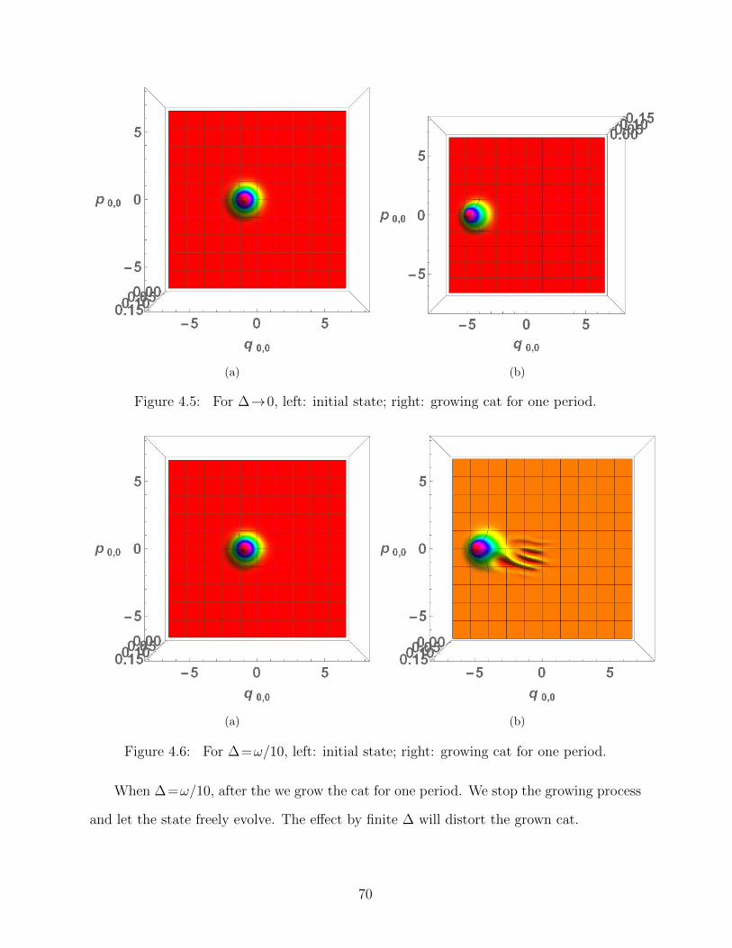
(a) (b)
Figure 4.5: For ∆→0, left: initial state; right: growing cat for one period.
(a) (b)
Figure 4.6: For ∆=ω/10, left: initial state; right: growing cat for one period.
When ∆=ω/10, after the we grow the cat for one period. We stop the growing process
and let the state freely evolve. The effect by finite ∆ will distort the grown cat.
70

(a)
Figure 4.7: For ∆=ω/10, grown cat evolves for 10 period, distorted.
But we can combat this with σz − π pulse. As mentioned in Section II, odd or even
number of pulses per period makes very big difference.
(a) (b)
Figure 4.8: For ∆=ω/10, grown cat evolves for 10 period, distortion corrected by 1 (left)
and 24 (right) pulses per period.
71

4.5 Chapter 4 Conclusion
In conclusion, we have analytically calculated the evolution of the quantum state in
the coupled qubitoscillator system, under a Hamiltonian of time–dependent coupling coef-
ficient, with zeroth order effect of small qubit frequency. We have introduced the concept
of dynamical energy eigenstate which is analogous to the regular energy eigenstate un-
der a time independent coupling coefficient, which tremendously simplifies the formula for
quantum state evolution. We have shown the result of the first order effect of small qubit
frequency. We have designed a mechanism to minimize the first order effect and demon-
strate its viability both analytically and numerically. We have also demonstrated how to
put our analytical result into practice and designed schemes realizable in experiment, in
order to increase the amplitude of the cat state.
We should again stress that although our original motivation of this work is the super-
conducting qubit–oscillator in deep strong coupling, our theory in fact applies to all system
with Hamiltonian described in Eq. (4.1.
4.6 Chapter 4 Supplementary Material: Detailed Derivation for Evolution un-
der Time–dependent Qubit-oscillator Coupling Coefficient with Infinites-
imal Qubit Frequency.
The Hamiltonian of the combined system of the qubit and the oscillator is
H(t)=~ω(a†a+1
2) + ~g(t)σz(a
† + a)− ~2
(∆σx + εσz), (4.25)
Now we take the limit of ε=0, ∆→0 (∆�ω). Under this limit the Hamiltonian is
now
H(t)=~ω(a†a+1
2) + ~g(t)σz(a
† + a). (4.26)
72

As a result, the energy eigenstates at time t are
|En±(t)〉= 1√2
(|σz+〉 D(−g(t)
ω) |n〉 ± |σz−〉 D(+
g(t)
ω) |n〉), (4.27)
The qubit state of |σz±〉 are defined as eigenstate of operator σz, with eigenvalue of
±1:
σz |σz±〉=± |σz±〉 (4.28)
In many experimental setups, we start from a stabilized g(tI) before changing it at
t= tI, at which time the system has been sufficiently relaxed to the ground state |E0+(tI)〉,
|E0+(tI)〉=1√2
(|σz+〉 |−g(tI)
ω〉+ |σz−〉 |+
g(tI)
ω〉) (4.29)
But here we start from a more general initial state:
|Φ(tI)〉= |σz±〉 D(∓ g(tI)
ω) |N〉 . (4.30)
We can choose particular ± and N , but the following calculation applies to all ± and
N . We can also see that with various choices of N and ±, |Φ(tI)〉 represents a complete
orthonormal basis regardless of the value of g(tI). By examining the evolution of initial
state |Φ(tI)〉 with all choices of ± and N , we can understand the evolution of any general
initial state, which itself can be expressed as a superposition of |Φ(tI)〉 with different ± and
N . Also note that in principle we can set g(tI) to any value, but sometimes we choose to
let g(tI)=g(tI). This is because it simplifies the expression if we have an energy eigenstate
as the initial state.
Now, Let us calculate the time evolution of the initial state |Φ(tI)〉. We divide the time
period of interest into f small segments, so that the entire period is divided by time points
73

tI, t1, t2, · · · , ti, ti+1, · · · , tF. Each segment is considered to be small enough so that, in a
single segment g(t) and H(t) do not change much and are treated as constants.
Therefore the final state at t= tF can be expressed as
|Φ(tF)〉=exp[−iH(tF)× (tF − tf−1)/~] · · · exp[−iH(tj)× (tj+1 − tj)/~] · · · exp[−iH(tI)× (t1 − tI)/~] |σz±〉 D(∓ g(tI)
ω) |N〉 .
(4.31)
Our task now is to solve for |Φ(tF)〉. At each time point t= tj, starting with t= tI, we
do the following procedures.
(1) We make the conjecture that, at any time point t= tj, the evolved state remains in
the form of
|Φ(tj)〉=eiφN±(tj) |σz±〉 D(∓ g(tj)
ω) |N〉 , (4.32)
where ± and N are the same as the initial state |Φ(tI)〉. This is obviously true at t= tI and
we will show later, by mathematical induction, that indeed at each time point the state
can be expressed in such form. The complex number g(tj) generally changes at different
time points, and a phase eiφn±(tj) can accumulate as well.
(2) To make the expression more compact, let τj = tj+1 − tj, gj =g(tj), gj = g(tj), Hj =
H(tj). The state at tj+1, evolving from the state at the previous time point tj, can be
expressed as follows:
|Φ(tj+1)〉=exp[−iH(tj)× (tj+1 − tj)/~] |Φ(tj)〉
=exp[−iH(tj)× (tj+1 − tj)/~] exp[iφN±(tj)]D(∓ g(tj)
ω) |σz±〉 |N〉
(4.33)
We move the phase term to the left hand side of the equation to avoid keep writing it.
74

exp[−iφN±(tj)] |Φ(tj+1)〉
=exp[−iH(tj)× (tj+1 − tj)/~]D(∓ g(tj)
ω) |σz±〉 |N〉
=exp[−iH(tj)τj/~]D(∓ g(tj)
ω) |σz±〉 |N〉
=exp[−iHjτj/~]D(∓ gjω
) |σz±〉 |N〉
=exp{−i[ω(a†a+1
2)± gj(a† + a)]τj}D(∓ gj
ω)
1√N !
(a†)N |σz±〉 |0〉
=exp{−i[ω(a†a+1
2)± gj(a† + a)]τj}
1√N !
(a† ±g∗jω
)ND(∓ gjω
) |σz±〉 |0〉
=exp[−i=[(g∗j − gj)gj]
ω2]
exp{−i[ω(a†a+1
2)± gj(a† + a)]τj}
1√N !
(a† ±g∗jω
)ND(∓gjω
)D(∓ gj − gjω
) |σz±〉 |0〉
=exp[−i=[(g∗j − gj)gj]
ω2] exp(−i1
2ωτj)
exp{−i[ω(a†a)± gj(a† + a)]τj}1√N !
[(a† ± gjω
)±g∗j − gjω
]ND(∓gjω
)D(∓ gj − gjω
) |σz±〉 |0〉
=exp[−i=[(g∗j − gj)gj]
ω2] exp(−i1
2ωτj)
exp{−i[ω(a†a)± gj(a† + a)]τj}1√N !
[(a† ± gjω
)±g∗j − gjω
]N
D(∓gjω
)∞∑
M=0
exp(−1
2| ∓ gj − gj
ω|2)
1√M !
(∓ gj − gjω
)M |σz±〉 |M〉
=exp[−i=[(g∗j − gj)gj]
ω2] exp(−i1
2ωτj)
exp{−i[ω(a†a)± gj(a† + a)]τj}1√N !
N∑p=0
(N
p
)(a† ± gj
ω)p(±
g∗j − gjω
)N−p
∞∑M=0
exp(−1
2| ∓ gj − gj
ω|2)
1√M !
(∓ gj − gjω
)MD(∓gjω
) |σz±〉 |M〉
(4.34)
75

Now let us digress a little and prove the following equations:
[ω(a†a)± gj(a† + a)]D(∓gjω
) |σz±〉 |M〉
=D(∓gjω
)[ω(a† ∓ gjω
)(a∓ gjω
)± gj(a† ∓gjω
+ a∓ gjω
)] |σz±〉 |M〉
=D(∓gjω
)(ωa†a− g2i
ω) |σz±〉 |M〉
=D(∓gjω
)(ωM − g2i
ω) |σz±〉 |M〉
=(ωM − g2i
ω)D(∓gj
ω) |σz±〉 |M〉 ,
(4.35)
and
[ω(a†a)± gj(a† + a), (a† ± gjω
)]
=[ω(a†a)± gj(a† + a)](a† ± gjω
)− (a† ± gjω
)[ω(a†a)± gj(a† + a)]
=ω(a† ± gjω
),
(4.36)
which leads to
[ω(a†a)± gj(a† + a), (a† ± gjω
)p]
=ω(a† ± gjω
)p(a† ± gjω
)p−1
=pω(a† ± gjω
)p.
(4.37)
Therefore,
[ω(a†a)± gj(a† + a)](a† ± gjω
)p
=(a† ± gjω
)p{[ω(a†a)± gj(a† + a)] + pω}.(4.38)
76

Therefore,
exp{−i[ω(a†a)± gj(a† + a)]τj}(a† ±gjω
)p
=(a† ± gjω
)p exp{−i[ω(a†a)± gj(a† + a) + pω]τj}.(4.39)
77

Now we are able to resume calculating Eq. (4.34)
exp[−iφN±(tj)] |Φ(tj+1)〉
=exp[−i=[(g∗j − gj)gj]
ω2] exp(−i1
2ωτj)
exp{−i[ω(a†a)± gj(a† + a)]τj}1√N !
N∑p=0
(N
p
)(a† ± gj
ω)p(±
g∗j − gjω
)N−p
∞∑M=0
exp(−1
2| ∓ gj − gj
ω|2)
1√M !
(∓ gj − gjω
)MD(∓gjω
) |σz±〉 |M〉
=exp[−i=[(g∗j − gj)gj]
ω2] exp(−i1
2ωτj)
1√N !
N∑p=0
(N
p
)(a† ± gj
ω)p exp{−i[ω(a†a)± gj(a† + a) + pω]τj}(±
g∗j − gjω
)N−p
∞∑M=0
exp(−1
2| ∓ gj − gj
ω|2)
1√M !
(∓ gj − gjω
)MD(∓gjω
) |σz±〉 |M〉
=exp[−i=[(g∗j − gj)gj]
ω2] exp(−i1
2ωτj)
1√N !
N∑p=0
(N
p
)[(a† ± gj
ω) exp(−iωτj)]p exp{−i[ω(a†a)± gj(a† + a)]τj}(±
g∗j − gjω
)N−p
∞∑M=0
exp(−1
2| ∓ gj − gj
ω|2)
1√M !
(∓ gj − gjω
)MD(∓gjω
) |σz±〉 |M〉
=exp[−i=[(g∗j − gj)gj]
ω2] exp(−i1
2ωτj)
1√N !
N∑p=0
(N
p
)[(a† ± gj
ω) exp(−iωτj)]p(±
g∗j − gjω
)N−p
∞∑M=0
exp(−1
2| ∓ gj − gj
ω|2)
1√M !
(∓ gj − gjω
)M exp{−i[ω(a†a)± gj(a† + a)]τj}D(∓gjω
) |σz±〉 |M〉
=exp[−i=[(g∗j − gj)gj]
ω2] exp(−i1
2ωτj)
1√N !
[(a† ± gjω
) exp(−iωτj)±g∗j − gjω
]N
∞∑M=0
exp(−1
2| ∓ gj − gj
ω|2)
1√M !
(∓ gj − gjω
)M exp[−i(ωM − g2i
ω)τj]D(∓gj
ω) |σz±〉 |M〉
(This equation continues to the next page)
(4.40)
78

exp[−iφN±(tj)] |Φ(tj+1)〉
=exp[−i=[(g∗j − gj)gj]
ω2] exp(−i1
2ωτj) exp(+i
g2i
ωτj)
1√N !
[(a† ± gjω
) exp(−iωτj)±g∗j − gjω
]N
D(∓gjω
)∞∑
M=0
exp(−1
2| ∓ gj − gj
ω|2)
1√M !
[∓ gj − gjω
exp(−iωτj)]M |σz±〉 |M〉
=exp[−i=[(g∗j − gj)gj]
ω2] exp(−i1
2ωτj) exp(+i
g2i
ωτj)
1√N !
[(a† ± gjω
) exp(−iωτj)±g∗j − gjω
]N
D(∓gjω
)D[∓ gj − gjω
exp(−iωτj)] |σz±〉 |0〉
=exp[−i=[(g∗j − gj)gj]
ω2] exp(−i1
2ωτj) exp(+i
g2i
ωτj) exp[i
=[(g∗j − gj)gjexp(iωτj)]
ω2]
1√N !
[(a† ± gjω
) exp(−iωτj)±g∗j − gjω
]N
D[∓gjω∓ gj − gj
ωexp(−iωτj)] |σz±〉 |0〉
=exp[−i=[(g∗j − gj)gj]
ω2] exp(−i1
2ωτj) exp(+i
g2i
ωτj) exp[i
=[(g∗j − gj)gjexp(iωτj)]
ω2]
D[∓gjω∓ gj − gj
ωexp(−iωτj)]
1√N !
[(a†∓gjω∓g∗j − gjω
exp(+iωτj)±gjω
) exp(−iωτj)±g∗j − gjω
]N |σz±〉 |0〉
=exp[−i=[(g∗j − gj)gj]
ω2] exp(−i1
2ωτj) exp(+i
g2i
ωτj) exp[i
=[(g∗j − gj)gjexp(iωτj)]
ω2]
D[∓gjω∓ gj − gj
ωexp(−iωτj)]
1√N !
[(a† ∓g∗j − gjω
exp(+iωτj)) exp(−iωτj)±g∗j − gjω
]N |σz±〉 |0〉
=exp[−i=[(g∗j − gj)gj]
ω2] exp(−i1
2ωτj) exp(+i
g2i
ωτj) exp[i
=[(g∗j − gj)gjexp(iωτj)]
ω2]
D[∓gjω∓ gj − gj
ωexp(−iωτj)]
1√N !
[a† exp(−iωτj)∓g∗j − gjω
±g∗j − gjω
]N |σz±〉 |0〉
=exp[−i=[(g∗j − gj)gj]
ω2] exp(−i1
2ωτj) exp(+i
g2i
ωτj) exp[i
=[(g∗j − gj)gjexp(iωτj)]
ω2]
D[∓gjω∓ gj − gj
ωexp(−iωτj)]
1√N !
[a† exp(−iωτj)]N |σz±〉 |0〉
=exp[−i=[(g∗j − gj)gj]
ω2] exp(−i1
2ωτj) exp(+i
g2i
ωτj) exp[i
=[(g∗j − gj)gjexp(iωτj)]
ω2] exp(−iNωτj)
D[∓gjω∓ gj − gj
ωexp(−iωτj)] |σz±〉 |N〉
(4.41)79

Therefore
|Φ(tj+1)〉=exp(ig2i
ωτj) exp[−i
={(g∗j − gj)gj[1− exp(iωτj)]}ω2
] exp[−i(N +1
2)ωτj] exp[iφN±(tj)]
D[∓gjω∓ gj − gj
ωexp(−iωτj)] |σz±〉 |N〉
(4.42)
Now recall that
|Φ(tj)〉=exp[iφN±(tj)] |σz±〉 D(∓ g(tj)
ω) |N〉 , (4.43)
Therefore we have proved, by mathematical induction, that apart from a global phase,
state of t= tj+1 also have the form of
|Φ(tj+1)〉=exp[iφN±(tj+1)] |σz±〉 D(∓ g(tj+1)
ω) |N〉 , (4.44)
with
g(tj+1)=g(tj) + [g(tj)− g(tj)] exp[−iω(tj+1 − tj)] (4.45)
and
φN±(tj+1)=g2i
ωτj −
={(g∗j − gj)gj[1− exp(iωτj)]}ω2
− (N +1
2)ωτj + φN±(tj) (4.46)
Since tj+1 − tj =τj→0,
g(tj+1)= g(tj)[1− iω(tj+1 − tj)]− g(tj)[−iω(tj+1 − tj)] (4.47)
80

and
φN±(tj+1)=g2i
ωτj +
=[i(g∗j − gj)gj]ω
τj − (N +1
2)ωτj + φN±(tj) (4.48)
Therefore,
g(tj+1)− g(tj)
tj+1 − tj= iω[g(tj)− g(tj)], (4.49)
which leads to
d
dtg(t)= iω(g(t)− g(t)). (4.50)
We can solve this differential equation.
g(t)= g(tI)e−iω(t−tI) + e−iω(t−tI)
t∫tI
iωg(t′)eiω(t′−tI)dt′. (4.51)
As the state evolves under changing g, the global phase φ(tF) will be accumulated and
the final state is going to be
|Φ(tF)〉=eiφ(tF)D(∓ g(tF)
ω) |σz±〉 |N〉 . (4.52)
where φ(tF)=tF∫tI
(=[i(g∗−g)g]ω
+ g2
ω− (N + 1
2)ω)dt and g= g(t) is given by Eq. (4.51).
These results are also presented previously in Section II, Eqs. (4.5, 4.6, 4.7, 4.8).
81

Chapter 5
Overall Conclusion
In conclusion, I have developed the multimode approach to this classical diffraction
problem, which is traditionally solved based Huygens-Fresnel principle and Kirchhoff’s
diffraction formula. Compared to Kirchhoff’s diffraction formula and its approximation,
the multimode approach has a neater mathematical structure and simpler formalism. In
practice, the multimode approach also significantly lightens the computational burden and
provides a better and easier mechanism for precision control. Numerical simulation is
employed to demonstrate these advantages of the multimode approach to classical diffrac-
tion. Further exploration is also made to demonstrate the more efficient way to apply the
multimode approach.
The multimode approach is also applied to investigate the quantum diffraction problem.
The theory of quantization of Gaussian beams is developed to address the essential issue
of regarding the transformation of the operators amongst various Gaussian beam modes,
which determines how the multimode quantum states will evolve and interact. This is a
significant improvement upon method of the using plane waves to approximate Gaussian
beams, of which the disadvantage is that such approximation requires certain conditions,
such as, when the beam waist and Rayleigh range can be treated as much larger than the
typical width and depth of the experiment, which are not always satisfied, which will result
in inaccurate approximation. The multimode approach to the quantum diffraction has
opened up new opportunities to investigate quantum effect of almost all Gaussian beam
based models. The theoretical prediction derived from numerical simulations qualitatively
agrees with our experimental data published providing strong evidence of the effectiveness
of our method.
The work on superconducting qubit and oscillator with time depending coupling co-
efficient g(t), first order correction for small ∆, and π pulses is also presented. For the
system of superconducting qubitoscillator circuit in deep strong coupling regime, the en-
82

ergy ground state and first excited state are both so called the Schrdingers cat states, which
have important applications in both in quantum science and technology such as quantum
communication and computing. The evolution of the quantum state under a changing
coupling coefficient and the distortion effect on the cat state due to the finite qubit energy
are investigated. An analytical calculation has been done and also numerical simulations
are shown to verify our calculation.
83

References[1] Z. Xiao, R. N. Lanning, M. Zhang, I. Novikova, E. E. Mikhailov, and J. P. Dowling,
Phys. Rev. A 96, 023829 (2017).
[2] M. Zhang, R. N. Lanning, Z. Xiao, J. P. Dowling, I. Novikova, and E. E. Mikhailov,Phys. Rev. A 93, 013853 (2016).
[3] R. N. Lanning, Z. Xiao, M. Zhang, I. Novikova, E. E. Mikhailov, and J. P. Dowling,Phys. Rev. A 96, 013830 (2017).
[4] M. Zhang, M. A. Guidry, R. N. Lanning, Z. Xiao, J. P. Dowling, I. Novikova, andE. E. Mikhailov, Phys. Rev. A 96, 013835 (2017).
[5] J. D. Jackson, Classical electrodynamics (John Wiley & Sons, 2007).
[6] M. Born and E. Wolf, Principles of optics: electromagnetic theory of propagation,interference and diffraction of light (Elsevier, 2013).
[7] C. J. Bouwkamp, Rep. Prog. Phys. 17, 35 (1954).
[8] A. Sommerfeld, Lectures on theoretical physics: Optics (Academic Press, 1954).
[9] G. O. Olaofe, J. Opt. Soc. A. 60, 1654 (1970).
[10] R. G. Schell and G. Tyras, J. Opt. Soc. A. 61, 31 (1971).
[11] J. Campbell and L. DeShazer, J. Opt. Soc. A. 59, 1427 (1969).
[12] P. Belland and J. Crenn, Appl. Opt. 21, 522 (1982).
[13] A. Siegman, Lasers (University Science Books, Sausalito CA, 1986) p. 647.
[14] S. Zhang and T. Tamir, J. Opt. Soc. A. A 6, 1368 (1989).
[15] J. M. Liu, Opt. Lett. 7, 196 (1982).
[16] P. Belland and J. P. Crenn, Appl. Opt. 21, 522 (1982).
[17] J. E. Pearson, T. C. McGill, S. Kurtin, and A. Yariv, J. Opt. Soc. A. 59, 1440 (1969).
[18] K. Uehara and H. Kikuchi, Appl. Phys. B 48, 125 (1989).
[19] M. A. Porras, Phys. Rev. E 58, 1086 (1998).
[20] S. S. R. Oemrawsingh, J. A. W. Van Houwelingen, E. R. Eliel, J. P. Woerdman, E. J. K.Verstegen, J. G. Kloosterboer, and G. W. ’t Hooft, Appl. Opt. 43, 688 (2004).
[21] N. Passilly, F. Treussart, R. Hierle, R. de Saint Denis, K. Aıt-Ameur, and J.-F. Roch,J. Opt. Soc. A. A 22, 984 (2005).
84

[22] V. Perinova and A. Luks, J. Mod. Opt. 53, 659 (2006).
[23] N. Treps, U. Andersen, B. Buchler, P. K. Lam, A. Maitre, H.-A. Bachor, and C. Fabre,Phys. Rev. Lett. 88, 203601 (2002).
[24] N. Treps, N. Grosse, W. P. Bowen, C. Fabre, H.-A. Bachor, and P. K. Lam, Science301, 940 (2003).
[25] M. Lassen, G. Leuchs, and U. L. Andersen, Phys. Rev. Lett. 102, 163602 (2009).
[26] K. Banaszek, A. B. URen, and I. A. Walmsley, Opt. Lett. 26, 1367 (2001).
[27] N. Corzo, A. M. Marino, K. M. Jones, and P. D. Lett, Opt. Express 19, 21358 (2011).
[28] J. Janousek, K. Wagner, J.-F. Morizur, N. Treps, P. K. Lam, C. C. Harb, and H.-A.Bachor, Nature Photonics 3, 399 (2009).
[29] M. Beck, Phys. Rev. Lett. 84, 5748 (2000).
[30] A. La Porta and R. E. Slusher, Phys. Rev. A 44, 2013 (1991).
[31] C. Kim and P. Kumar, Phys. Rev. Lett. 73, 1605 (1994).
[32] B. Chalopin, F. Scazza, C. Fabre, and N. Treps, Opt. Express 19, 4405 (2011a).
[33] L. Lopez, B. Chalopin, A. R. de la Souchere, C. Fabre, A. Maıtre, and N. Treps, Phys.Rev. A 80, 043816 (2009).
[34] B. Chalopin, F. Scazza, C. Fabre, and N. Treps, in European Quantum ElectronicsConference (Optical Society of America, 2011) p. EA1 1.
[35] M. I. Kolobov, Rev. Mod. Phys. 71, 1539 (1999).
[36] M. I. Kolobov, C. Fabre, P. Scotto, P. Colet, and M. San Miguel, in Coherence andQuantum Optics VIII (Springer, 2003) pp. 173–184.
[37] B. Chalopin, F. Scazza, C. Fabre, and N. Treps, Phys. Rev. A 81, 061804 (2010).
[38] A. Vaziri, G. Weihs, and A. Zeilinger, J. Opt. B: Quantum and Semiclassical Optics.4, S47 (2002).
[39] C. Lupo, V. Giovannetti, S. Pirandola, S. Mancini, and S. Lloyd, Phys. Rev. A 85,062314 (2012).
[40] M. Zhang, J. Soultanis, I. Novikova, and E. E. Mikhailov, Opt. Lett. 38, 4833 (2013).
[41] T. Horrom, R. Singh, J. P. Dowling, and E. E. Mikhailov, Phys. Rev. A 86, 023803(2012).
[42] U. Leonhardt, Measuring the Quantum State of Light, Vol. 22 (Cambridge universitypress, 1997) pp. 31,62,74.
85

[43] C. Gerry and P. Knight, Introductory Quantum Optics. (Cambridge University Press,2005) pp. 138,162,185,184,144.
[44] X. Q. Yu, P. Xu, Z. D. Xie, J. F. Wang, H. Y. Leng, J. S. Zhao, S. N. Zhu, and N. B.Ming, Phys. Rev. Lett. 101, 233601 (2008).
[45] M. Barbieri, F. De Martini, G. Di Nepi, and P. Mataloni, Phys. Rev. Lett. 92, 177901(2004).
[46] J. P. Torres, A. Alexandrescu, S. Carrasco, and L. Torner, Opt. Lett. 29, 376 (2004).
[47] J. F. Clauser and M. A. Horne, Phys. Rev. D 10, 526 (1974).
[48] M. Genovese, Phys. Rep. 413, 319 (2005).
[49] C. F. Wildfeuer, A. P. Lund, and J. P. Dowling, Phys. Rev. A 76, 052101 (2007).
[50] C. K. Hong, Z. Y. Ou, and L. Mandel, Phys. Rev. Lett. 59, 2044 (1987).
[51] E. Karimi, D. Giovannini, E. Bolduc, N. Bent, F. M. Miatto, M. J. Padgett, andR. W. Boyd, Phys. Rev. A 89, 013829 (2014).
[52] S. P. Walborn, A. N. de Oliveira, S. Padua, and C. H. Monken, Phys. Rev. Lett. 90,143601 (2003).
[53] S. P. Walborn, W. A. T. Nogueira, A. N. de Oliveira, S. Padua, and C. H. Monken,Mod. Phys. Lett. B 19, 1 (2005).
[54] J. C. F. Matthews, K. Poulios, J. D. A. Meinecke, A. Politi, A. Peruzzo, N. Ismail,K. Worhoff, M. G. Thompson, and J. L. O’Brien, Scientific Reports 3 (2013).
[55] I. Chiorescu, P. Bertet, K. Semba, Y. Nakamura, C. Harmans, and J. Mooij, Nature431, 159 (2004).
[56] A. Wallraff, D. I. Schuster, A. Blais, L. Frunzio, R.-S. Huang, J. Majer, S. Kumar,S. M. Girvin, and R. J. Schoelkopf, Nature 431, 162 (2004).
[57] M. Devoret, S. Girvin, and R. Schoelkopf, Annalen der Physik 16, 767 (2007).
[58] T. Niemczyk, F. Deppe, H. Huebl, E. Menzel, F. Hocke, M. Schwarz, J. Garcia-Ripoll,D. Zueco, T. Hummer, E. Solano, et al., Nature Phys. 6, 772 (2010).
[59] P. Forn-Dıaz, J. Lisenfeld, D. Marcos, J. J. Garcıa-Ripoll, E. Solano, C. Harmans,and J. Mooij, Phys. Rev. Lett. 105, 237001 (2010).
[60] F. Yoshihara, T. Fuse, S. Ashhab, K. Kakuyanagi, S. Saito, and K. Semba, NaturePhys. 13, 44 (2017).
[61] S. Ashhab and F. Nori, Phys. Rev. A 81, 042311 (2010).
[62] J. Casanova, G. Romero, I. Lizuain, J. Garcıa-Ripoll, and E. Solano, Phys. Rev. Lett.105, 263603 (2010).
86

Appendix: Permission
87

Vita
Zhihao Xiao attended University of Science and Technology of China from 2004 to 2011
and earned the degrees of B.S. and M.S. in theoretical physics. He conducted his research
under Dr. Wen-ge Wang on dynamical decoupling. He joined Hearne Institute for Theo-
retical Physics and Department of Physics and Astronomy at Louisiana State University in
2011 pursuing a PhD degree under the supervision of Dr. Hwang Lee and Dr. Jonathan P.
Dowling. He worked as a lab instructor and he is currently working as a research assistant.
He is now a PhD candidate. His research areas include quantization of multimode Gaussian
beam, classical diffraction theory and superconducting qubit–oscillator circuit.
88