multilevel modeling with latent variables using mplus · 7 cluster-specific regressions yij = ß0j...
TRANSCRIPT

1
Multilevel Modeling With LatentVariables Using Mplus
Linda K. MuthénBengt Muthén
Copyright © Muthén & Muthénwww.statmodel.com
2
84Multilevel Two-Part Growth Modeling
52Multilevel Estimation
7Multilevel Regression Analysis
57Multivariate Modeling of Family Members
101Multilevel Discrete-Time Survival Analysis
54Practical Issues Related To The Analysis Of Multilevel Data
17Numerical Integration
3General Latent Variable Modeling Framework
32Twolevel Factor Analysis22Twolevel Path Analysis
61Twin Modeling
42Twolevel SEM
66Multilevel Growth Models63Multilevel Mixture Modeling
103References
85Multilevel Growth Mixture Modeling
5Analysis With Multilevel Data
Table Of Contents

3
General Latent Variable Modeling Framework
4
General Latent Variable Modeling Framework

5
Used when the data have been obtained by cluster samplingand/or unequal probability sampling to avoid biases inparameter estimates, standard errors, and tests of model fitand to learn about both within- and between-clusterrelationships.
Analysis Considerations
• Sampling perspective• Aggregated modeling – SUDAAN
• TYPE=COMPLEX– Stratification, sampling weights, clustering
(Asparouhov, 2005)
Analysis With Multilevel Data
6
• Multilevel perspective• Disaggregated modeling – multilevel modeling
• TYPE = TWOLEVEL• Multivariate modeling
• TYPE = GENERAL
Analysis Areas
• Multilevel regression analysis• Multilevel path analysis• Multilevel factor analysis• Multilevel SEM• Multilevel latent class analysis• Multilevel growth modeling• Multilevel 2-part growth modeling• Multilevel growth mixture modeling
Analysis With Multilevel Data (Continued)
7
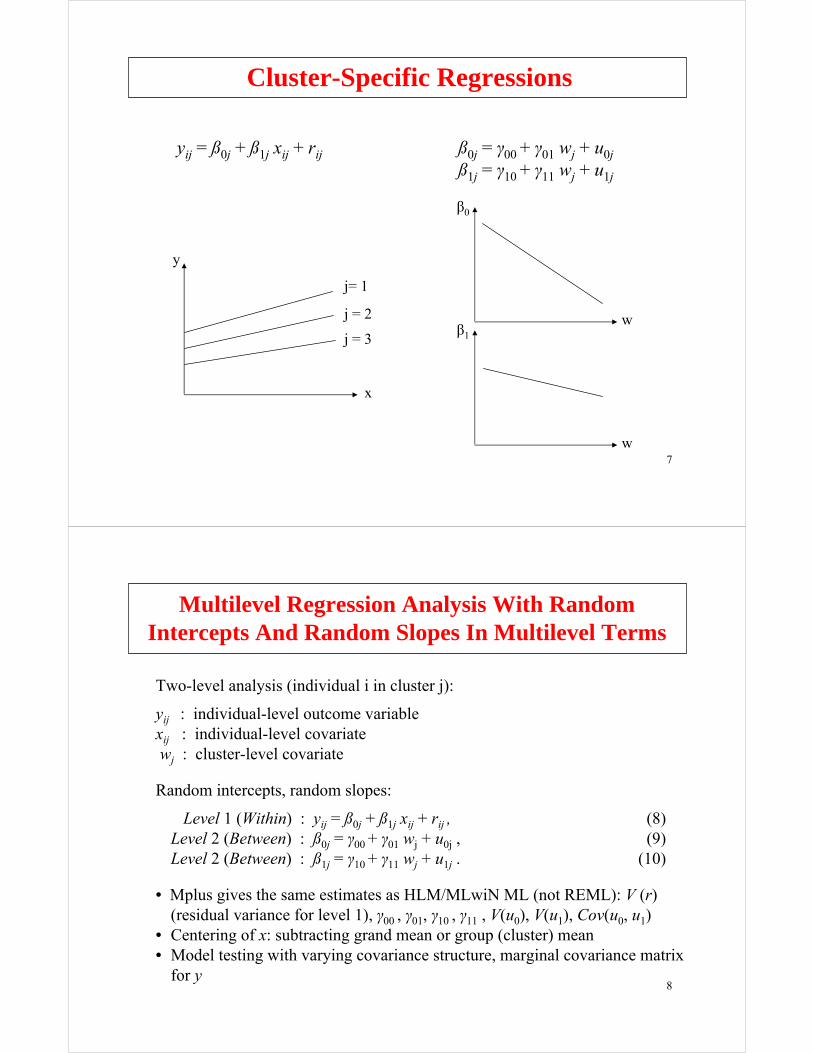
Cluster-Specific Regressions
yij = ß0j + ß1j xij + rij ß0j = γ00 + γ01 wj + u0jß1j = γ10 + γ11 wj + u1j
j= 1
j = 2
j = 3
y
x
β1
w
β0
w
8
Two-level analysis (individual i in cluster j):
yij : individual-level outcome variablexij : individual-level covariatewj : cluster-level covariate
Random intercepts, random slopes:
Level 1 (Within) : yij = ß0j + ß1j xij + rij , (8)Level 2 (Between) : ß0j = γ00 + γ01 wj + u0j , (9)Level 2 (Between) : ß1j = γ10 + γ11 wj + u1j . (10)
• Mplus gives the same estimates as HLM/MLwiN ML (not REML): V (r) (residual variance for level 1), γ00 , γ01, γ10 , γ11 , V(u0), V(u1), Cov(u0, u1)
• Centering of x: subtracting grand mean or group (cluster) mean• Model testing with varying covariance structure, marginal covariance matrix
for y
Multilevel Regression Analysis With RandomIntercepts And Random Slopes In Multilevel Terms

9
BetweenWithin
m92
s1
s2
mean_ses
catholic
per_adva
private
s1
s2
stud_ses
female
m92
10
TITLE: multilevel regression
DATA: FILE IS completev2.dat;! National Education Longitudinal Study (NELS)FORMAT IS f8.0 12f5.2 f6.3 f11.4 23f8.2f18.2 f8.0 4f8.2;
VARIABLE: NAMES ARE school r88 m88 s88 h88 r90 m90 s90 h90 r92m92 s92 h92 stud_ses f2pnlwt transfer minor coll_aspalgebra retain aca_back female per_mino hw_timesalary dis_fair clas_dis mean_col per_high unsafe num_frie teaqual par_invo ac_track urban size rural private mean_ses catholic stu_teac per_adva tea_excetea_res;
USEV = m92 female stud_ses per_adva private catholic mean_ses;
!per_adva = percent teachers with an MA or higher
WITHIN = female stud_ses;BETWEEN = per_adva private catholic mean_ses;MISSING = blank;CLUSTER = school;CENTERING = GRANDMEAN (stud_ses);
Input For Multilevel Regression Model

11
ANALYSIS: TYPE = TWOLEVEL RANDOM MISSING;
MODEL: %WITHIN%s1 | m92 ON female;s2 | m92 ON stud_ses;
%BETWEEN%s1 WITH m92; s2 WITH m92;m92 s1 s2 ON per_adva private catholic mean_ses;
OUTPUT: TECH8 SAMPSTAT;
Input For Multilevel Regression Model
12
1046868028
26234380636411267574
4264068595
2679087842
1995
1821968254
85508935699531735719
8304898582
4502511662
52654
7479183234
68153109044439593859
6140793469
8126327159
75862
144649471
316465095
984619208
654074040266512
417434570
89863
157736842
7400516701283525784
8308575498
5624156214
20770109104755580675
60835661257738134139
83390867335088020048
4
87745854
976163496
7219370718
5
3968581069
6770817543
4141211517
3
21474828606028138454
289239326611
N = 10,933Summary of Data
Number of clusters 902
Size (s) Cluster ID with Size s
Output Excerpts For Multilevel RegressionModel (Continued)

13
3157289842365327234
9951642
16515678324458626622091882634292597105661925
76909847288288727
94802471205366012786313617730
19091678359359981919
50626700249794758687
228746032815426
917
75115
80553
369886411795703459
460363143
32
43
2423
1092685125226330237741
Average cluster size 12.187Estimated Intraclass Correlations for the Y Variables
IntraclassVariable Correlation
M92 0.107
Output Excerpts For Multilevel RegressionModel (Continued)
14
Tests of Model Fit
LoglikelihoodH0 Value -39390.404
Information CriteriaNumber of Free parameters 21Akaike (AIC) 78822.808Bayesian (BIC) 78976.213Sample-Size Adjusted BIC 78909.478
(n* = (n + 2) / 24)
-0.9440.780-0.736CATHOLIC
Within LevelResidual Variances
61.4421.14970.577M92Between Level
-0.5420.428-0.232MEAN_SES
-0.1590.844-0.134PRIVATE0.1000.8410.084PER_ADVA
S1 ON
Model ResultsEstimates S.E. Est./S.E.
Output Excerpts For Multilevel RegressionModel (Continued)

15
4.0661.4115.740S1
-2.6120.562-1.467CATHOLIC3.6400.2831.031MEAN_SES
0.2680.7270.195PER_ADVA1.3581.1081.505PRIVATE
Intercepts
-4.4271.007-4.456M92S1 WITH
S2 WITH
1.1780.6500.765CATHOLIC
M92 ON
0.3220.3990.128M92
9.8140.3993.912MEAN_SES
-1.6880.507-0.856S1128.2310.42854.886M92
Residual Variances13.2080.3094.075S2
0.5830.5270.307S2
8.6491.0038.679M92
-2.6770.706-1.890PRIVATE2.5870.5211.348PER_ADVA
S2 ON
Output Excerpts For Multilevel RegressionModel (Continued)
16
• In single-level modeling random slopes ßi describe variation across individuals i,
yi = αi + ßi xi + εi , (100)αi = α + ζ0i , (101)ßi = ß + ζ1i , (102)
Resulting in heteroscedastic residual variancesV ( yi | xi ) = V ( ßi ) + . (103)
• In two-level modeling random slopes ßj describe variation across clusters j
yij = aj + ßj xij + εij , (104)aj = a + ζ0j , (105)ßj = ß + ζ1j , (106)
A small variance for a random slope typically leads to slow convergence of the ML-EM iterations. This suggests respecifying the slope as fixed.
Mplus allows random slopes for predictors that are• Observed covariates• Observed dependent variables (Version 3)• Continuous latent variables (Version 3)
2ix θ
Random Slopes

17
Numerical Integration
Numerical integration is needed with maximum likelihoodestimation when the posterior distribution for the latent variablesdoes not have a closed form expression. This occurs for models withcategorical outcomes that are influenced by continuous latentvariables, for models with interactions involving continuous latentvariables, and for certain models with random slopes such asmultilevel mixture models.
When the posterior distribution does not have a closed form, it isnecessary to integrate over the density of the latent variables multiplied by the conditional distribution of the outcomes given the latent variables. Numerical integration approximates this integration by using a weighted sum over a set of integration points (quadrature nodes) representing values of the latent variable.
18
Numerical Integration (Continued)
Numerical integration is computationally heavy and thereby time-consuming because the integration must be done at each iteration, both when computing the function value and when computing the derivative values. The computational burden increases as a function of the number of integration points, increases linearly as a function of the number of observations, and increases exponentially as a function of the dimension of integration, that is, the number of latent variables for which numerical integration is needed.

19
Practical Aspects Of Numerical Integration
• Types of numerical integration available in Mplus with or without adaptive quadrature• Standard (rectangular, trapezoid) – default with 15 integration
points per dimension• Gauss-Hermite• Monte Carlo
• Computational burden for latent variables that need numerical integration• One or two latent variables Light• Three to five latent variables Heavy• Over five latent variables Very heavy
20
• Suggestions for using numerical integration• Start with a model with a small number of random effects and
add more one at a time• Start with an analysis with TECH8 and MITERATIONS=1 to
obtain information from the screen printing on the dimensions of integration and the time required for one iteration and with TECH1 to check model specifications
• With more than 3 dimensions, reduce the number of integration points to 5 or 10 or use Monte Carlo integration with the default of 500 integration points
• If the TECH8 output shows large negative values in the column labeled ABS CHANGE, increase the number of integration points to improve the precision of the numerical integration and resolve convergence problems
Practical Aspects Of Numerical Integration (Continued)

21
Numerical Integration
Wei
ght
Wei
ght
Points
Points
Nonparametric Estimation Of TheRandom Effect Distribution
22
Twolevel Path Analysis With Categorical Outcomes

23
femalemothedhomeresexpectlunchexpelarrest
droptht7hisp
blackmath7math10
hsdrop
femalemothedhomeresexpectlunchexpelarrest
droptht7hispblackmath7
hsdrop
math10
Logistic Regression Path Model
24
math10
hsdrop
BetweenWithin
Two-Level Path Analysis
femalemothedhomeresexpectlunchexpelarrest
droptht7hispblackmath7
math10
hsdrop
25
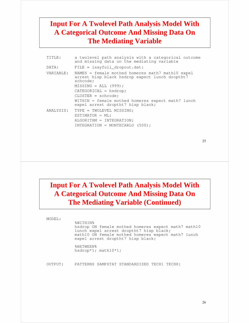
FILE = lsayfull_dropout.dat;DATA:
TYPE = TWOLEVEL MISSING;ESTIMATOR = ML;ALGORITHM = INTEGRATION;INTEGRATION = MONTECARLO (500);
ANALYSIS:
NAMES = female mothed homeres math7 math10 expel arrest hisp black hsdrop expect lunch droptht7 schcode;MISSING = ALL (999);CATEGORICAL = hsdrop;CLUSTER = schcode;WITHIN = female mothed homeres expect math7 lunch expel arrest droptht7 hisp black;
VARIABLE:
a twolevel path analysis with a categorical outcome and missing data on the mediating variable
TITLE:
Input For A Twolevel Path Analysis Model WithA Categorical Outcome And Missing Data On
The Mediating Variable
26
PATTERNS SAMPSTAT STANDARDIZED TECH1 TECH8;OUTPUT:
%WITHIN%hsdrop ON female mothed homeres expect math7 math10 lunch expel arrest droptht7 hisp black;math10 ON female mothed homeres expect math7 lunch expel arrest droptht7 hisp black;
%BETWEEN%hsdrop*1; math10*1;
MODEL:
Input For A Twolevel Path Analysis Model WithA Categorical Outcome And Missing Data On
The Mediating Variable (Continued)

27
Output Excerpts A Twolevel Path Analysis Model With A Categorical Outcome And Missing Data
On the Mediating Variable
Summary Of DataNumber of patterns 2Number of clusters 44
143101120
109112122
141303102146308103138106307305304
Cluster ID with Size s
4342
39383613
44
40
Size (s)
45
41
12
28
Output Excerpts A Twolevel Path Analysis Model With A Categorical Outcome And Missing Data
On the Mediating Variable (Continued)
30289
121581195910473
105123131117124111
115309
135145142137127126108140144
Cluster ID with Size s
118147
110
5755
51504947
93
13630152
Size (s)
118
53
46

29
Model Results
-0.340-0.4312.6650.2124.2011.324
-2.706-0.754-3.756-1.401-2.4571.887
0.2530.2740.2840.3210.2250.0060.0110.0150.0650.0550.1030.171
-0.013-0.086-0.086BLACK-0.016-0.118-0.118HISP0.0740.7570.757DROPTHT70.0070.0680.068ARREST0.1210.9470.947EXPEL0.0740.0080.008LUNCH
-0.197-0.031-0.031MATH10-0.055-0.011-0.011MATH7-0.159-0.244-0.244EXPECT-0.061-0.077-0.077HOMERES-0.121-0.253-0.253MOTHED0.0770.3230.323FEMALE
HSDROP ON
Est./S.E.S.E. StdYXStdEstimates
Output Excerpts A Twolevel Path Analysis Model With A Categorical Outcome And Missing Data
On the Mediating Variable (Continued)
Within Level
30
-0.503-0.689-1.358-3.353-1.567-2.30840.1236.0914.1691.222
-2.110
0.7330.7281.0491.0220.8250.0170.0230.1620.1360.2150.398
-0.009-0.369-0.369BLACK-0.010-0.501-0.501HISP-0.022-1.424-1.424DROPTHT7-0.054-3.426-3.426ARREST-0.026-1.293-1.293EXPEL-0.059-0.039-0.039LUNCH0.6970.9400.940MATH70.1000.9850.985EXPECT0.0700.5680.568HOMERES0.0200.2630.263MOTHED
-0.031-0.841-0.841FEMALEMATH10 ON
Est./S.E.S.E. StdYXStdEstimates
Output Excerpts A Twolevel Path Analysis Model With A Categorical Outcome And Missing Data
On the Mediating Variable (Continued)

31
3.0112.150
-1.920
7.632
28.683
1.2480.133
0.560
1.340
2.162
1.0003.7573.757MATH101.0000.2860.286HSDROP
Variances-1.076HSDROP$1
Thresholds5.27610.22610.226MATH10
MeansBetween Level
0.34162.01062.010MATH10Residual Variances
Est./S.E.S.E. StdYXStdEstimates
Output Excerpts A Twolevel Path Analysis Model With A Categorical Outcome And Missing Data
On the Mediating Variable (Continued)
32
Twolevel Factor Analysis With Categorical Outcomes

33
Within
u1 u2 u3 u4
fb
Between
u1 u2 u3 u4
fw
34
TYPE = TWOLEVEL;ESTIMATION = ML;ALGORITHM = INTEGRATION;
ANALYSIS:
%WITHIN%fw BY u1@1u2 (1)u3 (2)u4 (3)u5 (4)u6 (5);
MODEL:
FILE = catrep1.dat;DATA:NAMES ARE u1-u6 clus;CATEGORICAL = u1-u6;CLUSTER = clus;
VARIABLE:
this is an example of a two-level factor analysis model with categorical outcomes
TITLE:
Input For A Two-Level Factor Analysis ModelWith Categorical Outcomes

35
TECH1 TECH8;OUTPUT:
%BETWEEN%fb BY u1@1u2 (1)u3 (2)u4 (3)u5 (4)u6 (5);
Input For A Two-Level Factor Analysis ModelWith Categorical Outcomes
λ fij = λ (f j + f ij)B W
36
Tests Of Model Fit
7440.217Sample-Size Adjusted BIC(n* = (n + 2) / 24)
7418.235Akaike (AIC)
Loglikelihood
-3696.117HO Value
Bayesian (BIC)
Number of Free Parameters
Information Criteria
13
7481.505
Output Excerpts Two-Level Factor AnalysisModel With Categorical Outcomes

37
Model Results
4.360
6.4396.4496.4416.4376.2640.000
0.191
0.1780.1850.1640.1690.1460.000
0.834FWVariances
1.143U61.191U51.058U41.087U30.915U21.000U1
FW BY
Est./S.E.S.E.Estimates
Output Excerpts Two-Level Factor AnalysisModel With Categorical Outcomes (Continued)
Within Level
38Variances
-0.2090.102-0.021U6$1
3.562
-0.315-0.652-0.1560.007
-2.150
6.4396.4496.4416.4376.2640.000
0.139
0.1050.0980.1000.0910.096
0.1780.1850.1640.1690.1460.000
-0.033U5$1-0.064U4$1-0.016U3$10.001U2$1
-0.206U1$1Thresholds
1.143U61.191U51.058U4
0.496FB
1.087U30.915U21.000U1
FB BY
Est./S.E.S.E.Estimates
Output Excerpts Two-Level Factor AnalysisModel With Categorical Outcomes (Continued)Between Level

39
y1
y2
y3
y4
y5
y6
fbw
Within Between
y1
y2
y3
y4
y5
y6
fw1
fw2
x1
x2
Two-Level Factor Analysis with Covariates
40
• The Data—National Education Longitudinal Study (NELS:88)
• Base year Grade 8—followed up in Grades 10 and 12
• Student sampled within 1,035 schools—approximately 26 students per school
• Variables—reading, math, science, history-citizenship-geography, and background variables
• Data for the analysis—reading, math, science, history-citizenship-geography, gender, individual SES, school SES, and minority status
NELS Data
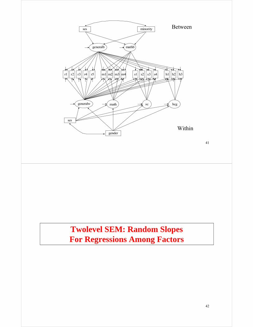
41
Between
Within
generalb mathb
ses minority
r1 r2 r3 r4 r5 m1 m2 m3 m4 s1 s2 s3 s4 h1 h2 h3
generalw math sc hcg
ses
gender
42
Twolevel SEM: Random SlopesFor Regressions Among Factors

43
Between
Within
f1w
y1
y2
y4
y3
f2w
y5
y6
y8
y7
s
f1b
y1
y2
y4
y3
f2b
y5
y6
y8
y7
x s
44
FILE = etaeta3.dat;DATA:
TYPE = TWOLEVEL RANDOM MISSING;ALGORITHM = INTEGRATION;
ANALYSIS:
NAMES ARE y1-y8 x clus;CLUSTER = clus;BETWEEN = x;
VARIABLE:
a twolevel SEM with a random slopeTITLE:
Input For A Twolevel SEM With A Random Slope

45TECH1 TECH8;OUTPUT:
%WITHIN%f1w BY y1@1y2 (1)y3 (2)y4 (3);f2w BY y5@1y6 (4)y7 (5)y8 (6);s | f2w ON f1w;
%BETWEEN%f1b BY y1@1y2 (1)y3 (2)y4 (3);f2b BY y5@1y6 (4)y7 (5)y8 (6);f2b ON f1b;s ON x;
MODEL:
Input For A Twolevel SEM With A Random Slope (Continued)
46
Tests Of Model Fit
25489.843Sample-Size Adjusted BIC(n* = (n + 2) / 24)
25439.114Akaike (AIC)
Loglikelihood
-12689.557HO Value
Bayesian (BIC)
Number of Free Parameters
Information Criteria
30
25585.122
Output Excerpts Twolevel SEMWith A Random Slope

47
Model Results
F1W WITH0.0000.0000.000F2W
F2W BY0.0000.0001.000Y5
34.4170.0280.978Y635.1740.0301.049Y738.0900.0261.008Y8
Within Level
26.88423.59328.5970.000
0.0370.0410.0350.000
1.001Y40.978Y30.992Y21.000Y1
F1W BY
Est./S.E.S.E.Estimates
Output Excerpts Twolevel SEMWith A Random Slope (Continued)
48
16.1910.0580.941Y717.8350.0601.076Y8
16.8540.0560.949Y217.4060.0601.052Y318.1740.0530.971Y418.1870.0571.039Y518.2920.0581.062Y6
15.517
9.14412.325
0.063
0.0630.082
0.979Y1Residual Variances
0.580F2W1.016F1W
Variances Est./S.E.)S.E.(Estimates
Output Excerpts Twolevel SEMWith A Random Slope (Continued)

49
F2B ON2.2480.0800.180F1B
F2B BY0.0000.0001.000Y5
34.4170.0280.978Y635.1740.0301.049Y738.0900.0261.008Y8
Between Level
26.88423.59328.5970.000
0.0370.0410.0350.000
1.001Y40.978Y30.992Y21.000Y1
F1B BY
Output Excerpts Twolevel SEMWith A Random Slope (Continued)
Est./S.E.)S.E.(Estimates
50
4.2110.0560.237F2B
5.9000.0960.568F1BVariances
Residual Variances
10.6040.0730.777S
4.7560.0880.420S
-0.0170.065-0.001Y40.4750.0620.030Y5
-0.1290.064-0.008Y60.6350.0640.041Y70.0350.0710.002Y8
S ON
-1.034-0.175-1.560
12.150
0.0670.0640.063
0.082
-0.069Y3-0.011Y2-0.099Y1
Intercepts0.999X
Output Excerpts Twolevel SEMWith A Random Slope (Continued)
Est./S.E.)S.E.(Estimates

51
y1 y2 y3 y4
iw sws
Student (Within)
w
s ib sb
y1 y2 y3 y4
School (Between)
Multilevel Modeling With A RandomSlope For Latent Variables
52
Estimators• Muthén’s limited information estimator (MUML) – random
intercepts• ESTIMATOR = MUML• Muthén’s limited information estimator for unbalanced data• Maximum likelihood for balanced data
• Full-information maximum likelihood (FIML) – random intercepts and random slopes• ESTIMATOR = ML, MLR, MLF• Full-information maximum likelihood for balanced and
unbalanced data• Robust maximum likelihood estimator• MAR missing data• Asparouhov and Muthén
Multilevel Estimation, Testing, Modification,And Identification

53
Tests of Model Fit• MUML – chi-square, robust chi-square, CFI, TLI,
RMSEA, and SRMR• FIML – chi-square, robust chi-square, CFI, TLI,
RMSEA, and SRMR• FIML with random slopes – no tests of model fit
Model Modification• MUML – modification indices not available• FIML – modification indices available
Model identification is the same as for CFA for both thebetween and within parts of the model.
Multilevel Estimation, Testing, Modification,And Identification (Continued)
54
Size Of The Intraclass Correlation
• Small intraclass correlations can be ignored but important information about between-level variability may be missed by conventional analysis
• The importance of the size of an intraclass correlation depends on the size of the clusters
• Intraclass correlations are attenuated by individual-level measurement error
• Effects of clustering not always seen in intraclasscorrelations
Practical Issues Related To TheAnalysis Of Multilevel Data

55
Within-Level And Between-Level Variables
• Variables measured on the within-level can be used in both the between-level and within-level parts of the model or only in the within-level part of the model (WITHIN=)
• Variables measured on the between-level can be used only in the between-level part of the model (BETWEEN=)
Sample Size
• There should be at least 30-50 between-level units (clusters)
• Clusters with only one observation are allowed
Practical Issues Related To TheAnalysis Of Multilevel Data (Continued)
56
• Explore SEM model using the sample covariance matrix from the total sample
• Estimate the SEM model using the pooled-within sample covariance matrix
• Investigate the size of the intraclass correlations and DEFF’s
• Explore the between structure using the estimated between covariance matrix
• Estimate and modify the two-level model suggested by the previous steps
Steps In SEM Multilevel AnalysisFor Continuous Outcomes
57
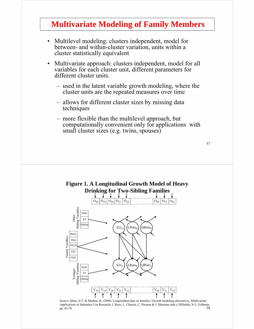
Multivariate Modeling of Family Members
• Multilevel modeling: clusters independent, model for between- and within-cluster variation, units within a cluster statistically equivalent
• Multivariate approach: clusters independent, model for all variables for each cluster unit, different parameters for different cluster units.
– used in the latent variable growth modeling, where the cluster units are the repeated measures over time
– allows for different cluster sizes by missing data techniques
– more flexible than the multilevel approach, but computationally convenient only for applications with small cluster sizes (e.g. twins, spouses)
58
Figure 1. A Longitudinal Growth Model of Heavy Drinking for Two-Sibling Families
Source: Khoo, S.T. & Muthen, B. (2000). Longitudinal data on families: Growth modeling alternatives. Multivariate Applications in Substance Use Research, J. Rose, L. Chassin, C. Presson & J. Sherman (eds.), Hillsdale, N.J.: Erlbaum, pp. 43-78.
O18
S21O LRateO QRateO
O19 O20 O21 O22 O30 O31 O32
Y18 Y19 Y20 Y21 Y22 Y30 Y31 Y32
Male
ES
HSDrp
Black
Hisp
FH123
FH1
FH23
Male
ES
HSDrp
S21Y LRateY QRateY
Old
er
Sib
ling
Var
iabl
es
Fam
ily
Var
iabl
es
You
nger
S
ibli
ng V
aria
bles

59
s21o BY o18-o32@1;lrateo BY o18@0 o19@1 o20@2 o21@3 o22@4 o23@5 o24@6 o25@7 o26@8 o27@9 o28@10 o29@11 o30@12 o31@13 o32@14;qrateo BY o18@0 o19@1 o20@4 o21@9 o22@16 o23@25 o24@36 o25@49 o26@64 o27@81 o28@100 o29@121 o30@144 o31@169 o32@196;s21y BY y18-y32@1;lratey BY y18@0 y19@1 y20@2 y21@3 y22@4 y23@5 y24@6 y25@7 y26@8 y27@9 y28@10 y29@11 y30212 y31@13 y32@14;qratey BY y18@0 y19@1 y20@4 y21@9 y22@16 y23@25 y24@36 y25@49 y26@64 y27@81 y28@100 y29@121 y30@144 y31@169 y32@196;s21o ON omale oes ohsdrop black hisp fh123 fh1 fh23;221y ON ymale yes yhsdrop black hisp fh123 fh1 fh23;s21y ON s21o;lratey ON s21o lrateo;qratey ON s21o lrateo qrateo;[o18-y32@0 s21o-qratey];
MODEL:
NAMES ARE o18-o32 y18-y32 omale oes ohsdrop ymale yoesyhsdrop black hisp fh123 fh1 hf123;
VARIABLE:
FILE IS multi.dat;DATA:
Multivariate Modeling Of Family DataOne Observation Per Family
TITLE:
Input For Multivariate ModelingOf Family Data
60
!New Version 3 Language For Growth Models
Input For Multivariate ModelingOf Family Data (Continued)
s21o lrateo qrateo | o18@0 o19@1 o20@2 o21@3 o22@4 o23@5 o24@6 o25@7 o26@8 o27@9 o28@10 o29@11 o30@12o31@13 o32@14;s21y lratey qratey | y18@0 y19@1 y20@2 y21@3 y22@4 y23@5 y24@6 y25@7 y26@8 y27@9 y28@10 y29@11 y30@12y31@13 y32@14;s12o ON omale oes ohsdrop black hisp fh123 fh1 fh23;221y ON ymale yes yhsdrop black hisp fh123 fh1 fh23;s21y ON s21o;lratey ON s21o lrateo;qratey ON s21o lrateo qrateo;
!MODEL

61
Twin Modeling
62
y1
C1 E1A1
a c e
y2
C2 E2A2
a c e
1.0 for MZ 1.00.5 for DZ
Twin1 Twin2
63
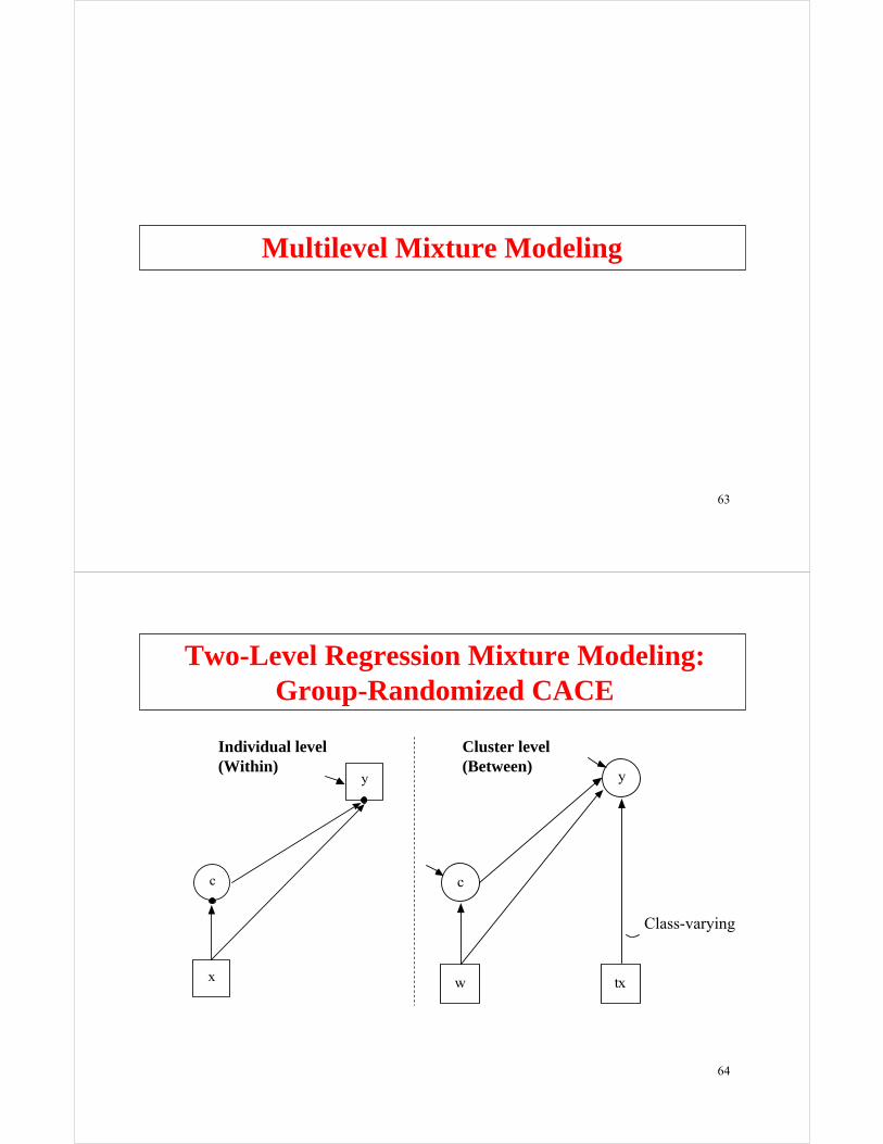
Multilevel Mixture Modeling
64
Individual level(Within)
Cluster level(Between)
Class-varying
y
c
x
c
w
y
tx
Two-Level Regression Mixture Modeling:Group-Randomized CACE

65
c
u2 u3 u4 u5 u6u1
x
f
c#1
w
c#2
Within Between
Two-Level Latent Class Analysis
66
Multilevel Growth Models

67
Growth Modeling Approached in Two Ways:Data Arranged As Wide Versus Long
yti = ii + si x timeti + εti
ii regressed on wisi regressed on wi
• Wide: Multivariate, Single-Level Approach
• Long: Univariate, 2-Level Approach (cluster = id)
Within Between
time ys i
y
i s
w
w
i
s
68
Growth Modeling Approached in Two Ways:Data Arranged As Wide Versus Long (Continued)
• Wide (one person):
t1 t2 t3 t1 t2 t3
Person i: id y1 y2 y3 x1 x2 x3 w
• Long (one cluster):
Person i: t1 id y1 x1 wt2 id y2 x2 wt3 id y3 x3 w

69
Time point t, individual i, cluster j.
ytij : individual-level, outcome variablea1tij : individual-level, time-related variable (age, grade)a2tij : individual-level, time-varying covariatexij : individual-level, time-invariant covariatewj : cluster-level covariate
Three-level analysis (Mplus considers Within and Between)
Level 1 (Within) : ytij = π0ij + π1ij a1tij + π2tij a2tij + etij , (1)
π 0ij = ß00j + ß01j xij + r0ij ,π 1ij = ß10j + ß11j xij + r1ij , (2)π 2tij = ß20tj + ß21tj xij + r2tij .
ß00j = γ000 + γ001 wj + u00j ,ß10j = γ100 + γ101 wj + u10j ,ß20tj = γ200t + γ201t wj + u20tj , (3)ß01j = γ010 + γ011 wj + u01j ,ß11j = γ110 + γ111 wj + u11j ,ß21tj = γ2t0 + γ2t1 wj + u2tj .
Level 2 (Within) :
Level 3 (Between) :
Three-Level Modeling In Multilevel Terms
70
Within Between
iw
x
y1
sw
y2 y3 y4
ib
w
y1
sb
y2 y3 y4
Two-Level Growth Modeling(3-Level Modeling)

71
iw
mothed
sw
ib
math7 math8
sb
math9 math10
mothed homeres
homeres
72
Input For LSAY Two-Level Growth ModelWith Free Time Scores And Covariates
FILE IS lsay98.dat;FORMAT IS 3f8 f8.4 8f8.2 3f8 2f8.2;
DATA:
NAMES ARE cohort id school weight math7 math8 math9 math10 att7 att8 att9 att10 gender mothed homeres; USEOBS = (gender EQ 1 AND cohort EQ 2);MISSING = ALL (999);USEVAR = math7-math10 mothed homeres;CLUSTER = school;
VARIABLE:
TYPE = TWOLEVEL;ESTIMATOR = MUML;
ANALYSIS:
LSAY two-level growth model with free time scores and covariates
TITLE:
73
SAMPSTAT STANDARDIZED RESIDUAL;OUTPUT
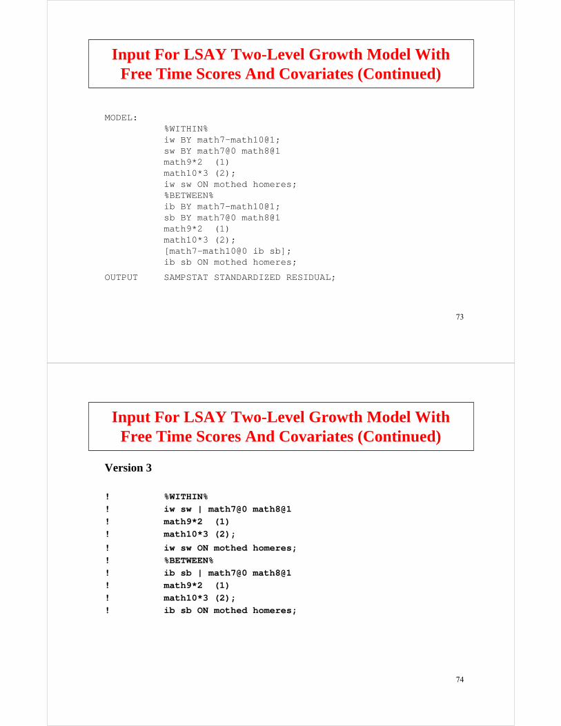
%WITHIN%iw BY math7-math10@1;sw BY math7@0 math8@1math9*2 (1)math10*3 (2);iw sw ON mothed homeres;%BETWEEN%ib BY math7-math10@1;sb BY math7@0 math8@1math9*2 (1)math10*3 (2);[math7-math10@0 ib sb];ib sb ON mothed homeres;
MODEL:
Input For LSAY Two-Level Growth Model WithFree Time Scores And Covariates (Continued)
74
math9*2 (1)!iw sw | math7@0 math8@1!
iw sw ON mothed homeres;!
math10*3 (2);!
ib sb | math7@0 math8@1!%BETWEEN%!
math10*3 (2);!math9*2 (1)!
ib sb ON mothed homeres;!
%WITHIN%!
Input For LSAY Two-Level Growth Model WithFree Time Scores And Covariates (Continued)
Version 3

75
Output Excerpts LSAY Two-Level Growth ModelWith free Time Scores And Covariates
14313730314712419
30511191091028
1037
1221051611611013810615
11813414
1281331461011311714118
307142129
304
112
132136114
6
20
21
Summary of DataNumber of clusters 50
Size (s) Cluster ID with Size s
76
Output Excerpts LSAY Two-Level Growth ModelWith free Time Scores And Covariates (Continued)
30240
117301261232511924
115331352910827
1043430939
308139121127145
140144120
232221
Size (s) Cluster ID with Size s
Average cluster size 18.627Estimated Intraclass Correlations for the Y Variables
0.165MATH10
0.168MATH90.149MATH80.199MATH7
VariableIntraclassCorrelationVariable
IntraclassCorrelation
IntraclassCorrelationVariable
77
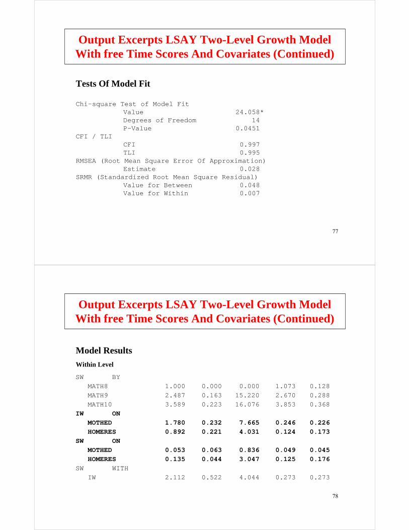
Tests Of Model Fit
Chi-square Test of Model FitValue 24.058*Degrees of Freedom 14P-Value 0.0451
CFI / TLICFI 0.997TLI 0.995
RMSEA (Root Mean Square Error Of Approximation)Estimate 0.028
SRMR (Standardized Root Mean Square Residual)Value for Between 0.048Value for Within 0.007
Output Excerpts LSAY Two-Level Growth ModelWith free Time Scores And Covariates (Continued)
78
Output Excerpts LSAY Two-Level Growth ModelWith free Time Scores And Covariates (Continued)
Model Results
Within Level
SW ON0.1730.1244.0310.2210.892HOMERES0.2260.2467.6650.2321.780MOTHED
IW ON0.3683.85316.0760.2233.589MATH100.2882.67015.2200.1632.487MATH90.1281.0730.0000.0001.000MATH8
SW BY
0.2730.2734.0440.5222.112IWSW WITH
0.1760.1253.0470.0440.135HOMERES0.0450.0490.8360.0630.053MOTHED

79
Output Excerpts LSAY Two-Level Growth ModelWith free Time Scores And Covariates (Continued)
0.9030.90315.3333.06947.060IW0.22624.82911.1332.23024.829MATH100.16614.23712.5781.13214.237MATH90.17412.29813.7710.89312.298MATH80.19712.7488.8881.43412.748MATH7
Residual Variances0.2030.2616.7090.0390.261MOTHED
HOMERES WITH
1.0001.97028.6430.0691.970HOMERES1.0000.84117.2170.0490.841MOTHED
Variances0.9640.9643.8790.2861.110SW
80
Output Excerpts LSAY Two-Level Growth ModelWith free Time Scores And Covariates (Continued)
Between Level
SB ON1.0112.1173.8761.8477.160HOMERES
-0.107-0.362-0.4742.587-1.225MOTHEDIB ON
0.1150.70416.0760.2233.589MATH100.1190.48815.2200.1632.487MATH90.0520.1960.0000.0001.000MATH8
SB BY
0.5750.5751.5380.2480.382IBSB WITH
0.0410.0860.0450.3730.017HOMERES1.4935.0731.5380.6470.995MOTHED
Estimates S.E. Est./S.E. Std StdYX

81
Output Excerpts LSAY Two-Level Growth ModelWith free Time Scores And Covariates (Continued)
6.5093.10850.3750.0623.108HOMERES7.8382.30753.2770.0432.307MOTHED
Means
1.0000.0873.8010.0230.087MOTHED1.0000.2284.0660.0560.228HOMERES
Intercepts9.9099.90912.5122.67833.510IB0.8300.8300.2100.7760.163SB
0.1250.1250.8451.6901.428IB0.0671.3952.7670.5041.395MATH100.0060.1050.4930.2130.105MATH90.0390.5442.0330.2680.544MATH80.1532.0593.7320.5522.059MATH7
Residual Variances0.7330.1035.4880.0190.103MOTHED
HOMERES WITH
Variances-1.321-1.321-0.7130.071-0.051SB
82
Output Excerpts LSAY Two-Level Growth ModelWith free Time Scores And Covariates (Continued)
R-SquareWithin Level
0.036SW
R-SquareLatentVariable
0.774MATH100.834MATH90.826MATH80.803MATH7
R-SquareObservedVariable
0.097IW
83
Output Excerpts LSAY Two-Level Growth ModelWith free Time Scores And Covariates (Continued)
R-SquareBetween Level
0.23207E+01UndefinedSW
R-SquareLatentVariable
0.933MATH100.994MATH90.961MATH80.847MATH7
R-SquareObservedVariable
0.875IW
84
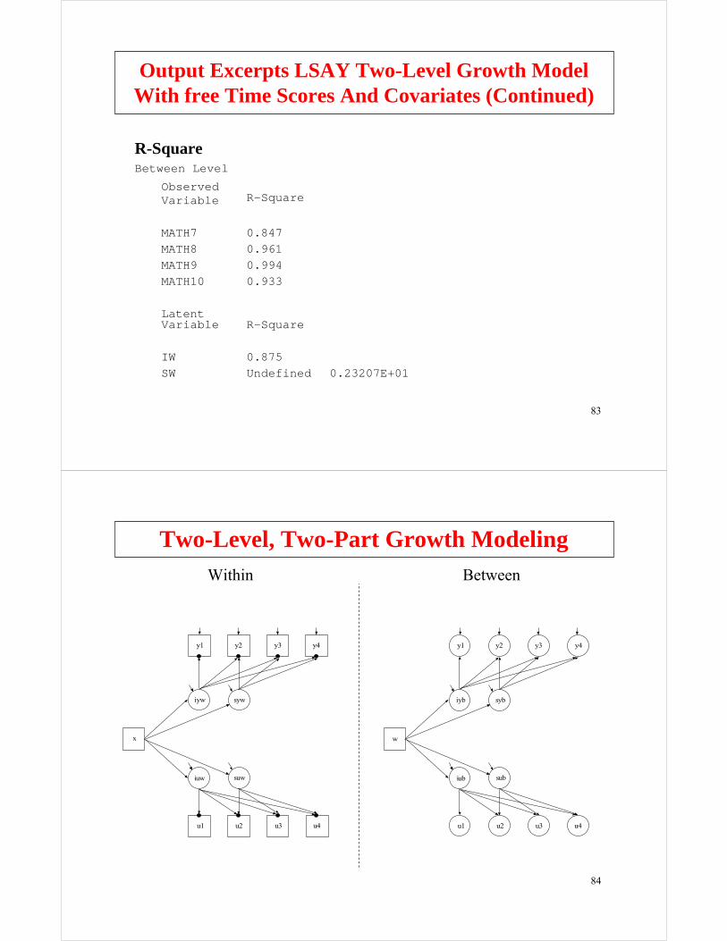
Two-Level, Two-Part Growth Modeling
Within Between
y1 y2 y3 y4
iuw
iyw syw
u1 u2 u3 u4
x
suw
y1 y2 y3 y4
iub
iyb syb
u1 u2 u3 u4
w
sub

85
Multilevel Growth Mixture Modeling
86
Mat
h A
chie
vem
ent
Poor Development: 20% Moderate Development: 28% Good Development: 52%
69% 8% 1%Dropout:
7 8 9 10
4060
8010
0
Grades 7-107 8 9 10
4060
8010
0
Grades 7-107 8 9 10
4060
8010
0
Grades 7-10
Growth Mixture Modeling:LSAY Math Achievement Trajectory ClassesAnd The Prediction Of High School Dropout

87
High SchoolDropout
Female
Hispanic
Black
Mother’s Ed.
Home Res.
Expectations
Drop Thoughts
Arrested
Expelled
c
i s
Math7 Math8 Math9 Math10
ib sb
School-Level Covariates
cb hb
Multilevel Growth Mixture Modeling
88
FILE = lsayfull_Dropout.dat;DATA:
NAMES = female mothed homeres math7 math8 math9 math10 expel arrest hisp black hsdrop expect lunch mstratdroptht7;!lunch = % of students eligible for full lunch!assistance (9th)!mstrat = ratio of students to full time math!teachers (9th)MISSING = ALL (9999);CATEGORICAL = hsdrop;CLASSES = c (3);CLUSTER = schcode;WITHIN = female mothed homeres expect droptht7 expel arrest hisp black;BETWEEN = lunch mstrat;
VARIABLE:
multilevel growth mixture model for LSAY math achievement
TITLE:
Input For A Multilevel Growth Mixture ModelFor LSAY Math Achievement

89
TYPE = PLOT3;SERIES = math7-math10 (s);
PLOT:
SAMPSTAT STANDARDIZED TECH1 TECH8;OUTPUT:
TYPE = MIXTURE TWOLEVEL MISSING;ALGORITHM = INTEGRATION;
ANALYSIS:
lunch = lunch/100;mstrat = mstrat/1000;
DEFINE:
Input For A Multilevel Growth Mixture ModelFor LSAY Math Achievement (Continued)
90
%WITHIN%%OVERALL%i s | math7@0 math8@1 math9@2 math10@3;i s c#1 c#2 hsdrop ON female hisp black mothed homeresexpect droptht7 expel arrest;
%c#1%[i*40 s*1];math7-math10*20;i*13 s*3;
%c#2%[i*40 s*5];math7-math10*30;i*8 s*3;i s ON female hisp black mothed homeres expectdroptht7 expel arrest;
MODEL:
Input For A Multilevel Growth Mixture ModelFor LSAY Math Achievement (Continued)
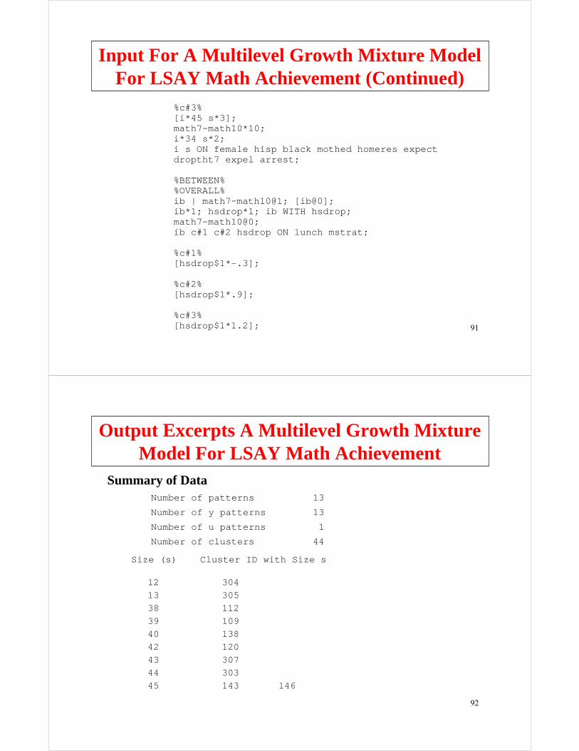
91
%c#3%[i*45 s*3];math7-math10*10;i*34 s*2;i s ON female hisp black mothed homeres expectdroptht7 expel arrest;
%BETWEEN%%OVERALL%ib | math7-math10@1; [ib@0];ib*1; hsdrop*1; ib WITH hsdrop;math7-math10@0;ib c#1 c#2 hsdrop ON lunch mstrat;
%c#1%[hsdrop$1*-.3];
%c#2%[hsdrop$1*.9];
%c#3%[hsdrop$1*1.2];
Input For A Multilevel Growth Mixture ModelFor LSAY Math Achievement (Continued)
92
Summary of Data
146143453034430743120421384010939112383051330412
Output Excerpts A Multilevel Growth MixtureModel For LSAY Math Achievement
1Number of u patterns
13Number of y patterns
44Number of clusters
13Number of patterns
Size (s) Cluster ID with Size s

93
11959
3028930994
126122
13514510512158
10473
1475711056
115118
1231411035513712711730154
1241311081421405311113311813652
3081025110614448
10146
Output Excerpts A Multilevel Growth MixtureModel For LSAY Math Achievement (Continued)
94
MAXIMUM LOG-LIKELIHOOD VALUE FOR THE UNRESTRICTED (H1) MODEL IS -36393.088
THE STANDARD ERRORS OF THE MODEL PARAMETER ESTIMATES MAY NOT BE TRUSTWORTHY FOR SOME PARAMETERS DUE TO A NON-POSITIVE DEFINITE FIRST-ORDER DERIVATIVE PRODUCT MATRIX. THIS MAY BE DUE TO THE STARTING VALUES BUT MAY ALSO BE AN INDICATION OF MODEL NONIDENTIFICATION. THE CONDITION NUMBER IS -0.758D-16. PROBLEM INVOLVING PARAMETER 54.
THE NONIDENTIFICATION IS MOST LIKELY DUE TO HAVING MORE PARAMETERS THAN THE NUMBER OF CLUSTERS. REDUCE THE NUMBER OF PARAMETERS.
THE MODEL ESTIMATION TERMINATED NORMALLY
Output Excerpts A Multilevel Growth MixtureModel For LSAY Math Achievement (Continued)

95
Tests Of Model Fit
53053.464Sample-Size Adjusted BIC(n* = (n + 2) / 24)
52738.409Akaike (AIC)
Loglikelihood
-26247.205HO Value
Entropy
Bayesian (BIC)
Number of Free Parameters
Information Criteria
122
0.632
53441.082
Output Excerpts A Multilevel Growth MixtureModel For LSAY Math Achievement (Continued)
FINAL CLASS COUNTS AND PROPORTIONS OF TOTAL SAMPLE SIZE BASEDON ESTIMATED POSTERIOR PROBABILITIES
0.18380430.83877Class 20.523351226.72218Class 3
0.29285686.43905Class 1
96
Est./S.E.S.E. StdYXStdEstimatesModel Results
Output Excerpts A Multilevel Growth MixtureModel For LSAY Math Achievement (Continued)
-0.253-0.196-1.2670.328-0.416HSDROPIB WITH
-0.016-0.178-0.1201.478-0.178MSTRAT0.2901.0872.0040.5431.087LUNCH
HSDROP ON
-0.448-6.299-4.3313.086-13.365MSTRAT-0.176-0.851-1.3781.310-1.805LUNCH
IB ONCLASS 1Between Level

97
Output Excerpts A Multilevel Growth MixtureModel For LSAY Math Achievement (Continued)
0.0000.0000.0000.0000.000MATH90.0000.0000.0000.0000.000MATH10
0.0000.0000.0000.0000.000MATH80.0000.0000.0000.0000.000MATH7
0.7680.7683.4221.0103.456IB
0.9150.5502.5420.2160.550HSDROPResidual Variances
0.0000.0000.0000.0000.000IB0.0000.0000.0000.0000.000MATH100.0000.0000.0000.0000.000MATH90.0000.0000.0000.0000.000MATH80.0000.0000.0000.0000.000MATH7
Intercepts
98
Est./S.E.S.E.Estimates
Model Results
Output Excerpts A Multilevel Growth MixtureModel For LSAY Math Achievement (Continued)
2.8420.3841.093ARREST2.0680.3370.698EXPEL3.5830.4511.616DROPTHT7
-3.4060.074-0.251EXPECT0.8640.069-0.060HOMERES
-0.0280.106-0.003MOTHED2.3390.3850.900BLACK0.1330.7050.094HISP
-3.9980.188-0.751FEMALEC#1 ON
Within Level
LATENT CLASS REGRESSION MODEL PART
99
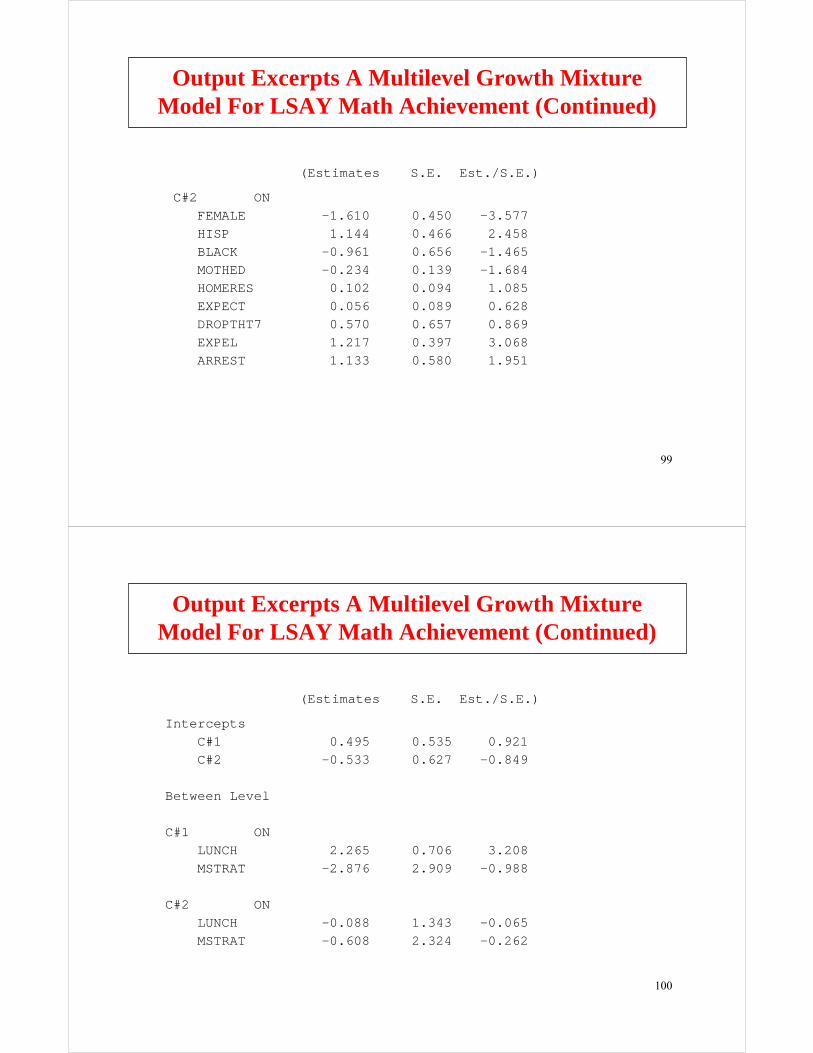
Est./S.E.)S.E.(Estimates
Output Excerpts A Multilevel Growth MixtureModel For LSAY Math Achievement (Continued)
1.9510.5801.133ARREST3.0680.3971.217EXPEL0.8690.6570.570DROPTHT70.6280.0890.056EXPECT1.0850.0940.102HOMERES
-1.6840.139-0.234MOTHED-1.4650.656-0.961BLACK2.4580.4661.144HISP
-3.5770.450-1.610FEMALEC#2 ON
100
Est./S.E.)S.E.(Estimates
Output Excerpts A Multilevel Growth MixtureModel For LSAY Math Achievement (Continued)
-0.0651.343-0.088LUNCHC#2 ON
-0.9882.909-2.876MSTRAT3.2080.7062.265LUNCH
-0.2622.324-0.608MSTRAT
C#1 ON
Between Level
-0.8490.627-0.533C#20.9210.5350.495C#1
Intercepts

101
Multilevel Discrete-Time Survival Analysis
• Muthén and Masyn (2005) in Journal of Educational and Behavioral Statistics
• Masyn dissertation
• Asparouhov and Muthén
102
Discrete-Time Survival Frailty Modeling
Within Between
u1 u2 u3 u4 u5
fwx
1 1 1 1 1
u1 u2 u3 u4 u5
fbw
1 1 1 1 1
103
References(To request a Muthén paper, please email [email protected].)
General
Asparouhov, T. (2005). Sampling weights in latent variable modeling. MplusWeb Notes: No. 7. Forthcoming in Structural Equation Modeling.
Analysis With Multilevel Data
Cross-sectional Data
Harnqvist, K., Gustafsson, J.E., Muthén, B. & Nelson, G. (1994). Hierarchical models of ability at class and individual levels. Intelligence, 18, 165-187. (#53)
Heck, R.H. (2001). Multilevel modeling with SEM. In G.A. Marcoulides & R.E. Schumacker (eds.), New Developments and Techniques in Structural Equation Modeling (pp. 89-127). Lawrence Erlbaum Associates.
Hox, J. (2002). Multilevel analysis. Techniques and applications. Mahwah, NJ: Lawrence Erlbaum.
Kaplan, D. & Elliott, P.R. (1997). A didactic example of multilevel structural equation modeling applicable to the study of organizations. Structural Equation Modeling: A Multidisciplinary Journal, 4, 1-24.
104
Kaplan, D. & Kresiman, M.B. (2000). On the validation of indicators of mathematics education using TIMSS: An application of multilevel covariance structure modeling. International Journal of Educational Policy, Research, and Practice, 1, 217-242.
Kreft, I. & de Leeuw, J. (1998). Introducing multilevel modeling. Thousand Oakes, CA: Sage Publications.
Longford, N.T., & Muthén, B. (1992). Factor analysis for clustered observations. Psychometrika, 57, 581-597. (#41)
Muthén, B. (1989). Latent variable modeling in heterogeneous populations. Psychometrika, 54, 557-585. (#24)
Muthén, B. (1990). Mean and covariance structure analysis of hierarchical data. Paper presented at the Psychometric Society meeting in Princeton, N.J., June 1990. UCLA Statistics Series 62. (#32)
Muthén, B. (1991). Multilevel factor analysis of class and student achievement components. Journal of Educational Measurement, 28, 338-354. (#37)
Muthén, B. (1994). Multilevel covariance structure analysis. In J. Hox & I. Kreft (eds.), Multilevel Modeling, a special issue of Sociological Methods & Research, 22, 376-398. (#55)
Muthén, B., Khoo, S.T. & Gustafsson, J.E. (1997). Multilevel latent variable modeling in multiple populations. (#74)
References (Continued)

105
References (Continued)Muthén, B. & Satorra, A. (1995). Complex sample data in structural equation
modeling. In P. Marsden (ed.), Sociological Methodology 1995, 216-316. (#59)
Raudenbush, S.W. & Bryk, A.S. (2002). Hierarchical linear models: Applications and data analysis methods. Second edition. Newbury Park, CA: Sage Publications.
Skinner, C.J., Holt, D. & Smith, T.M.F. (1989). Analysis of complex surveys. West Sussex, England, Wiley.
Snijders, T. & Bosker, R. (1999). Multilevel analysis. An introduction to basic and advanced multilevel modeling. Thousand Oakes, CA: Sage Publications.
Longitudinal Data
Khoo, S.T. & Muthén, B. (2000). Longitudinal data on families: Growth modeling alternatives. Multivariate Applications in Substance use Research, J. Rose, L. Chassin, C. Presson & J. Sherman (eds.), Hillsdale, N.J.: Erlbaum, pp. 43-78. (#79)
Masyn, K. E. (2003). Discrete-time survival mixture analysis for single and recurrent events using latent variables. Doctoral dissertation, University of California, Los Angeles.
106
References (Continued)
Muthén, B. (1997). Latent variable modeling with longitudinal and multilevel data. In A. Raftery (ed.) Sociological Methodology (pp. 453-480). Boston: Blackwell Publishers.
Muthén, B. (1997). Latent variable growth modeling with multilevel data. In M. Berkane (ed.), Latent Variable Modeling with Application to Causality(149-161), New York: Springer Verlag.
Muthén, B. & Masyn, K. (in press). Discrete-time survival mixture analysis. Journal of Educational and Behavioral Statistics, Spring 2005.
General
Mplus Analysis
Asparouhov, T. & Muthén, B. (2003a). Full-information maximum-likelihood estimation of general two-level latent variable models. In preparation.
Asparouhov, T. & Muthén, B. (2003b). Maximum-likelihood estimation in general latent variable modeling. In preparation.
Muthén, B. (2002). Beyond SEM: General latent variable modeling. Behaviormetrika, 29, 81-117.

107
References (Continued)
Muthén, B. & Asparouhov, T. (2003b). Advances in latent variable modeling, part II: Integrating continuous and categorical latent variable modeling using Mplus. In preparation.
Numerical integration
Aitkin, M. A general maximum likelihood analysis of variance components in generalized linear models. Biometrics, 1999, 55, 117-128.
Bock, R.D. & Aitkin, M. (1981). Marginal maximum likelihood estimation of item parameters: Application of an EM algorithm. Psychometrika, 46, 443-459.
General
Muthén, L. & Muthén, B. (1998-2003). Mplus User’s Guide. Los Angeles, CA: Muthén & Muthén.
Muthén, L.K. and Muthén, B. (2002). How to use a Monte Carlo study to decide on sample size and determine power. Structural Equation Modeling, 4, 599-620.
Lambert, D. (1992). Zero-inflated Poisson regression, with an application to defects in manufacturing. Technometrics, 34, 1-13.
108
References (Continued)
SEM
Latent variable interactions
Klein, A. & Moosbrugger, H. (2000). Maximum likelihood estimation of latent interaction effects with the LMS method. Psychometrika, 65, 457-474.
Indirect effects
MacKinnon, D.P., Lockwood, C.M., Hoffman, J.M., West, S.G. & Sheets, V. (2002). A comparison of methods to test mediation and other intervening variable effects. Psychological Methods, 7, 83-104.
Shrout, P.E. & Bolger, N. (2002). Mediation in experimental and nonexperimental studies: New procedures and recommendations. Psychological Methods, 7, 422-445.
Growth Modeling
Carlin, J.B., Wolfe, R., Brown, C.H., Gelman, A. (2001). A case study on the choice, interpretation and checking of multilevel models for longitudinal binary outcomes. Biostatistics, 2, 397-416.
109
References (Continued)
Duan, N., Manning, W.G., Morris, C.N. & Newhouse, J.P. (1983). A comparison of alternative models for the demand for medical care. Journal of Business and Economic Statistics, 1, 115-126.
Farrington, D.P. & West, D.J. (1990). The Cambridge study in delinquent development: A prospective longitudinal study of 411 males. In Criminality: Personality, Behavior, and Life History, edited by Hans-JurgenKernere and G. Kaiser. New York: Springer – Verlag.
Hedeker, D. (2000). A fully semi-parametric mixed-effects regression model for categorical outcomes. Presented at the Joint Statisticacl Meetings, Indianapolis, IN, 2000.
Hedeker, D. & Gibbons, R.D. (1994). A random-effects ordinal regression model for multilevel analysis. Biometrics, 50, 933-944.
Olsen, M.K. & Schafer, J.L. (2001). A two-part random effects model for semicontinuous longitudinal data. Journal of the American Statistical Association, 96, 730-745.
Raudenbush, S.w. & Bryk, A.S. (2002). Hierarchical linear models: Applications and data analysis methods. Second edition. Newbury Park, CA: Sage Publications.
Tubin, J. (1958). Estimation of relationships for limited dependent variables. Econometrica, 26, 24-36.
110
References (Continued)
Multilevel Modeling
Choi, K.C. (2002). Latent variable regression in a three-level hierarchical modeling framework: A fully Bayesian approach. Doctoral dissertation, University of California, Los Angeles.
Seltzer, M., Choi, K., Thum, Y.M. (2002). Examining relationships between where students start and how rapidly they progress: Implications for conducting analyses that help illuminate the distribution of achievement within schools. CSE Technical Report 560. CRESST, University of California, Los Angeles.
Mixture Modeling
Albert, P.A., McShane, L.M., Shih, J.H. & The US SCI Bladder Tumor Marker Network (2001). Latent class modeling approaches for assessing diagnostic error without a gold standard: With applications to p.53 immunohistochemical assays in bladder tumors. Biometrics, 57, 610-619.
Heinen, D. (1996). Latent class and discrete latent trait models: similarities and differences. Thousand Oakes, CA: Sage Publications.
111
References (Continued)
Land, K.C. (2001). Introduction to the special issue on finite mixture models. Sociological Methods & Research, 29, 275-281.
Lo, Mendell, & Rubin (2001). Testing the number of components in a normal mixture. Biometrika, 88, 767-778.
McLachlan, G.J. & Peel, D. (2000). Finite mixture models. New York: Wiley & Sons.
Muthén, B. (2001b). Two-part growth mixture modeling. Draft.Muthén, B. (2003a). Statistical and substantive checking in growth mixture
modeling. Psychological Methods, 8, 369-377.Muthén, B. (2003b). Latent variable analysis: Growth mixture modeling and
related techniques for longitudinal data. Forthcoming in D. Kaplan (ed.), Handbook of Quantitative Methodology for the Social Sciences, Sage Publications.
Muthén, B. (2003c). Advances in latent variable modeling of heterogeneous phenotypes. Presentation at NICA, May 2003.
Muthén, B. (2003d). Multilevel growth mixture modeling: Math achievement trajectory classes and high school dropout. Presentation at AERA, March 2003.
112
References (Continued)
Muthén, B., Kreuter, F. & Asparouhov, T. (2003). Applications of growth mixture modeling to non-normal outcomes. In preparation.
Muthén, B. & Masyn, K. (2001). Mixture discrete-time survival analysis. Submitted to Journal of Educational and Behavioral Statistics.
Muthén, B. & Shedden, K. (1999). Finite mixture modeling with mixture outcomes using the EM algorithm. Biometrics, 55, 463-469.
Nagin, D.S. & Land, K.C. (1993). Age, criminal careers, and population heterogeneity: Specification and estimation of a nonparametric, mixed Poisson model. Criminology, 31, 327-362.
Qu, Y., Tan, M., & Kutner, M.H. (1996). Random effects models in latent class analysis for evaluating accuracy of diagnostic tests. Biometrics, 52, 797-810.
Nagin, D.S. (1999). Analyzing developmental trajectories: A semi-parametric, group-based approach. Psychological Methods, 4, 139-157.
Roeder, K., Lynch, K.G., & Nagin, D.S. (1999). Modeling uncertainty in latent class membership: A case study in criminology. Journal of the American Statistical Association, 94, 766-776.

113
References (Continued)
Rumberger, R.W. & Larson, K.A. (1998). Student mobility and the increasedrisk of high school dropout. American Journal of Education, 107, 1-35.
Singer, J.D. & Willett, J.B. (1993). It’s about time: using discrete-time survival analysis to study duration and the timing of events. Journal of Educational Statistics, 18, 155-195.
Wang, C.P., Brown, C.H. & Bandeen-Roche, K. (2002). Residual diagnostics for growth mixture models: Examining the impact of a preventive intervention on multiple trajectories of aggressive behavior. Manuscript submitted for publication.
Yamamoto, K. & Gitomer, D. (1993). Application of a HYBRID model to a test of cognitive skill representation. In N. Frederiksen, R. Mislevy, and I Beijar (eds.), Test theory for new generation of tests. Hillsdale, N.J.: LEA.