multilead analysis of t-wave alternans in the electrocardiogram
TRANSCRIPT

Instituto Universitario de Investigación
en Ingeniería de Aragón
PhD Thesis
Multilead analysisof T-wave alternans
in the electrocardiogram
Análisis multiderivacional de alternancias de ondaT en la señal electrocardiográfica
Violeta Monasterio Bazán
Supervisor:Juan Pablo Martínez Cortés
June 2011

ii

ACKNOWLEDGMENTS
What a journey this has been! I would not have made it here withoutthe help, guidance, and support of many people. To all of them, I extendmy most sincere and heartfelt thanks.
To Juan Pablo Martínez, my PhD advisor. I am profoundly grateful forhis constant support, his patient guidance, and his brilliant ideas. Workingwith him has been a great opportunity to grow scientifically and personally,and it has also been a lot of fun thanks to his cheerful disposition. Lookingback at the last five years, I can say I’ve been very fortunate to have himas supervisor.
To Pablo Laguna, head of our research group. Pablo has always providedme with detailed feedback on my work, and has offered me sound advice onmultiple occasions. His contagious energy and enthusiasm for research havebeen great help along the way.
To Gari Clifford, from the Laboratory for Computational Physiology(MIT, Cambridge MA). He made me feel part of his group during my stayat MIT, and opened the door for new exciting opportunities.
To all the members of our research group, I am indebted for their helpand support. It has been a pleasure to collaborate with them and to learnfrom them. The more I travel around, the more convinced I am that it is aprivilege to be part of such a collaborative and supportive group.
To my friends inside and outside university: Clara, Dani, Zurdo, Chuso,Chúster, Alberto... thanks for putting up with me and my thesis! Havingyour support along the way has made it so much easier. In particular, Iwant to thank Michele and Ana for being the most fun labmates to sharethe final sprint with.
Por último, me gustaría dedicar este trabajo a mis padres Maite yManolo, a mi hermana Maite, y a mi compañero Viorreta. Ellos son siempremi mejor apoyo y mi ejemplo a seguir. Familia, ¡lo hemos conseguido!

iv

Contents
Abstract ix
Resumen xi
List of Figures xiii
List of Tables xxi
1 Introduction 1
1.1 Motivation of the thesis . . . . . . . . . . . . . . . . . . . . . 11.2 Background . . . . . . . . . . . . . . . . . . . . . . . . . . . . 2
1.2.1 The electrocardiogram . . . . . . . . . . . . . . . . . . 31.2.2 Cardiovascular diseases . . . . . . . . . . . . . . . . . 91.2.3 T-wave alternans . . . . . . . . . . . . . . . . . . . . . 10
1.3 Objectives and outline of the thesis . . . . . . . . . . . . . . . 11
2 Review of TWA analysis methods 15
2.1 Introduction . . . . . . . . . . . . . . . . . . . . . . . . . . . . 152.2 Methods for TWA analysis . . . . . . . . . . . . . . . . . . . 16
2.2.1 Spectral Method . . . . . . . . . . . . . . . . . . . . . 162.2.2 Modified Moving Average Method . . . . . . . . . . . 172.2.3 Correlation Method . . . . . . . . . . . . . . . . . . . 192.2.4 Intrabeat Average Method . . . . . . . . . . . . . . . . 192.2.5 Laplacian Likelihood Ratio Method . . . . . . . . . . 202.2.6 Recent Methods . . . . . . . . . . . . . . . . . . . . . 20
v

vi CONTENTS
2.3 Evaluation of methods . . . . . . . . . . . . . . . . . . . . . . 22
2.3.1 Methodological evaluation . . . . . . . . . . . . . . . . 22
2.3.2 Clinical evaluation . . . . . . . . . . . . . . . . . . . . 23
3 Common materials and methods 27
3.1 Introduction . . . . . . . . . . . . . . . . . . . . . . . . . . . . 27
3.2 Basic scheme for single-lead analysis . . . . . . . . . . . . . . 27
3.2.1 Preprocessing of the ECG signal . . . . . . . . . . . . 28
3.2.2 Detection and estimation of TWA . . . . . . . . . . . 29
3.3 General scheme for multilead analysis . . . . . . . . . . . . . 32
3.3.1 Preprocessing of the ECG signal . . . . . . . . . . . . 33
3.3.2 Signal transformation . . . . . . . . . . . . . . . . . . 34
3.3.3 Detection of TWA . . . . . . . . . . . . . . . . . . . . 35
3.3.4 Signal reconstruction . . . . . . . . . . . . . . . . . . . 35
3.3.5 Estimation of TWA . . . . . . . . . . . . . . . . . . . 37
3.3.6 Variations of the general scheme . . . . . . . . . . . . 37
3.4 Signal transformation techniques . . . . . . . . . . . . . . . . 39
3.4.1 Principal Component Analysis . . . . . . . . . . . . . 39
3.4.2 Periodic Component Analysis . . . . . . . . . . . . . . 40
3.4.3 Spectral Ratio Maximization . . . . . . . . . . . . . . 41
3.4.4 Independent Component Analysis . . . . . . . . . . . 42
3.5 ECG Databases . . . . . . . . . . . . . . . . . . . . . . . . . . 44
3.5.1 STAFF-III Database . . . . . . . . . . . . . . . . . . . 44
3.5.2 PTB Diagnostic ECG Database . . . . . . . . . . . . . 44
3.5.3 Stress Test Database . . . . . . . . . . . . . . . . . . . 45
3.5.4 Physionet TWA Database . . . . . . . . . . . . . . . . 45
3.5.5 MIT-BIH Noise Stress Test Database . . . . . . . . . 45
3.5.6 MUSIC database . . . . . . . . . . . . . . . . . . . . . 46
Appendix 3.A: GLRT and MLE derivation for the LLRM . . . . . 47
Appendix 3.B: Generalized eigenvalues and the Rayleigh quotient . 50
4 Evaluation of the multilead scheme based on

CONTENTS vii
Principal Component Analysis 51
4.1 Introduction . . . . . . . . . . . . . . . . . . . . . . . . . . . . 514.2 Data sets . . . . . . . . . . . . . . . . . . . . . . . . . . . . . 52
4.2.1 Simulated data . . . . . . . . . . . . . . . . . . . . . . 524.2.2 Stress test signals . . . . . . . . . . . . . . . . . . . . . 54
4.3 Methods for TWA analysis . . . . . . . . . . . . . . . . . . . 544.4 Results . . . . . . . . . . . . . . . . . . . . . . . . . . . . . . . 55
4.4.1 Detection performance . . . . . . . . . . . . . . . . . . 554.4.2 Estimation accuracy . . . . . . . . . . . . . . . . . . . 594.4.3 Comparison with the Spectral Method . . . . . . . . . 604.4.4 Application to stress test signals . . . . . . . . . . . . 65
4.5 Discussion . . . . . . . . . . . . . . . . . . . . . . . . . . . . . 674.6 Conclusions . . . . . . . . . . . . . . . . . . . . . . . . . . . . 73Appendix 4.A: Additional simulation results . . . . . . . . . . . . . 74
5 Evaluation of the multilead scheme based on Periodic Com-ponent Analysis 81
5.1 Introduction . . . . . . . . . . . . . . . . . . . . . . . . . . . . 815.2 Data sets . . . . . . . . . . . . . . . . . . . . . . . . . . . . . 82
5.2.1 Synthetic signals . . . . . . . . . . . . . . . . . . . . . 825.2.2 Real signals with added TWA . . . . . . . . . . . . . . 835.2.3 Stress test signals . . . . . . . . . . . . . . . . . . . . . 845.2.4 Signals from the Physionet TWA database . . . . . . 85
5.3 Methods for TWA analysis . . . . . . . . . . . . . . . . . . . 855.4 Results . . . . . . . . . . . . . . . . . . . . . . . . . . . . . . . 86
5.4.1 Detection performance . . . . . . . . . . . . . . . . . . 865.4.2 Estimation accuracy . . . . . . . . . . . . . . . . . . . 945.4.3 Comparison to other source separation techniques . . 945.4.4 Application to stress test signals . . . . . . . . . . . . 975.4.5 Application to the Physionet TWA database . . . . . 98
5.5 Discussion . . . . . . . . . . . . . . . . . . . . . . . . . . . . . 1005.6 Conclusions . . . . . . . . . . . . . . . . . . . . . . . . . . . . 104

viii CONTENTS
6 Analysis of TWA in ambulatory records 1056.1 Introduction . . . . . . . . . . . . . . . . . . . . . . . . . . . . 1056.2 Study population . . . . . . . . . . . . . . . . . . . . . . . . . 106
6.2.1 Follow-up and end-points . . . . . . . . . . . . . . . . 1076.3 Methods . . . . . . . . . . . . . . . . . . . . . . . . . . . . . . 107
6.3.1 Measurement of TWA . . . . . . . . . . . . . . . . . . 1076.3.2 Statistical analysis . . . . . . . . . . . . . . . . . . . . 111
6.4 Results . . . . . . . . . . . . . . . . . . . . . . . . . . . . . . . 1116.5 Discussion . . . . . . . . . . . . . . . . . . . . . . . . . . . . . 1176.6 Conclusions . . . . . . . . . . . . . . . . . . . . . . . . . . . . 119
7 Conclusions 1217.1 Summary and conclusions . . . . . . . . . . . . . . . . . . . . 1217.2 Future work . . . . . . . . . . . . . . . . . . . . . . . . . . . . 123
List of Acronyms 125
Bibliography 127

ABSTRACT
T-wave alternans (TWA) is a cardiac phenomenon related to the mech-anisms leading to ventricular arrhythmias and sudden cardiac death (SCD).It appears in the surface electrocardiogram (ECG) as a beat-to-beat alter-nation in the morphology of the repolarization, and its amplitude can beso low that it is imperceptible to the naked eye. Several signal processingmethods have been proposed to detect TWA in the ECG and to quantifyits amplitude. Most of them analyze each lead (channel) of the ECG in-dependently, and only basic multilead strategies are adopted in commercialTWA systems. However, the joint analysis of various ECG channels pro-vides additional information about the spatial and temporal distribution ofcardiac phenomena, which can be exploited to improve the detection andquantification of TWA in the ECG.
The objective of this thesis is to develop multilead schemes for TWAanalysis that improve the detection and quantification of TWA in the ECG,and that increase the clinical value of TWA as a risk index. The work carriedout to achieve this goal is divided in three parts: design of novel multileadschemes for TWA analysis, methodological validation of the proposed tech-niques, and clinical validation of the multilead scheme that presents the bestperformance.
The first part of the thesis introduces a general scheme for multileadanalysis of TWA. The proposed scheme is an extended version of a usualsingle-lead scheme with two additional stages, signal transformation and sig-nal reconstruction, which are included to increase the detectability of TWAand to improve the estimation of TWA amplitude and waveform. Varioustechniques are proposed for the transformation stage: principal componentanalysis (PCA), periodic component analysis (πCA), independent compo-nent analysis (ICA) and spectral ratio maximization (SRM). TechniquesπCA and ICA have been applied to TWA analysis for the first time in thiswork. SRM is a new technique developed in this work which exploits theperiodicity of TWA to increase its detectability in the transformed signal.
The general multilead scheme can be combined with any single-leadmethod which detects and estimates TWA in separate stages. Along thethesis, it is combined with the Laplacian Likelihood Ratio Method for TWAanalysis, and also with the Spectral Method for comparison. Several modifi-cations of the general scheme are also proposed for its adaptation to differentclinical settings.

x CONTENTS
The second part of the thesis presents the methodological evaluation ofthe multilead scheme based on the different transformation techniques. Thealternatives are compared in various simulation studies, in which synthetic,semi-synthetic and real signals with known TWA are analyzed. Differencesbetween schemes are quantified using common performance metrics suchas probability of detection and probability of false alarm, and also usingnew global measures of the bias and variance of the TWA estimation. Theimprovements in the detection performance and in the accuracy of TWAestimation over a single-lead scheme are quantified for all the multilead al-ternatives. Results show that using the periodicity as a criterion to separateTWA from noise is the best multilead strategy among the compared options.Among the periodicity-based schemes, the one with the best performanceis the πCA-based multilead scheme.
The last part of the thesis demonstrates that the improvements in TWAanalysis obtained with the πCA-based scheme, together with a new strategyfor computing global TWA indices, make it possible to stratify cardiac riskin Holter recordings without the need for visual validation. The methodpresented here allows a multilead, fully-automated computation of TWAmarkers of cardiac risk in ambulatory ECGs. Results from a clinical studyshow that the average TWA activity over a 24-hour period provides im-portant prognostic information in patients with chronic heart failure. Twonovel indices, AAI and AAI90, are proposed to quantify the average TWAactivity, and are found to independently predict the risk of cardiac deathand SCD.

RESUMEN Y CONCLUSIONES
Las alternancias de onda T (TWA) se definen como una alteración enla morfología de la repolarización que se repite cada dos latidos. Este fenó-meno cardíaco está relacionado con el riesgo de sufrir arritmias ventricularesmalignas que pueden conducir a la muerte súbita cardíaca. Actualmente, elanálisis de TWA en el electrocardiograma (ECG) se utiliza para estratificarel riesgo de sufrir arritmias ventriculares, y decidir si un paciente puedebeneficiarse de la implantación de un desfibrilador automático implantable.
La amplitud de las TWA puede ser muy baja, del orden de los micro-voltios, resultando indetectables a simple vista en el ECG, lo que dificultaen gran medida su detección. Existen diferentes métodos de procesado dela señal para detectar las TWA y estimar sus parámetros (amplitud, formade onda). El principal inconveniente de los métodos existentes es o bienuna alta sensibilidad a la presencia de componentes no alternantes de granamplitud, o bien una baja sensibilidad a las TWA de baja amplitud. Ha-bitualmente, estos métodos se aplican a cada derivación (canal) del ECGde manera independiente, es decir, siguiendo un esquema de análisis mono-derivacional. Sin embargo, el análisis conjunto de varios canales del ECGproporciona información adicional sobre la distribución espacial y tempo-ral de los fenómenos cardiacos, que se podría aprovechar para mejorar ladetección y la cuantificación de TWA.
El objetivo de esta tesis es desarrollar estrategias de análisis multideriva-cional que mejoren la detección y la cuantificación de TWA en el ECG, y queaumenten el valor clínico de las TWA como índice de riesgo. El trabajo de-sarrollado para conseguir este objetivo se divide en tres partes: propuesta denuevas estrategias de análisis multiderivacional para detectar y cuantificarTWA, validación metodológica de las estrategias propuestas, y validaciónclínica de la alternativa multiderivacional con mejores prestaciones.
En la primera parte de la tesis se propone un esquema general para elanálisis multiderivacional de TWA. El esquema propuesto se ha diseñadocomo una versión extendida de un esquema monoderivacional habitual, alque se le han añadido dos etapas de procesado adicionales: transformaciónde la señal y reconstrucción de la señal. Con estas etapas se consigue incre-mentar la detectabilidad de las TWA y mejorar la estimación de su amplitudy de su forma de onda. Se proponen diferentes técnicas para la transfor-mación de la señal: análisis de componentes principales (PCA), análisisde componentes periódicos (πCA), análisis de componentes independientes

xii CONTENTS
(ICA) y maximización del ratio espectral (SRM). Las técnicas πCA e ICA sehan aplicado al análisis de TWA por primera vez en este trabajo. La técnicaSRM es una nueva propuesta de esta tesis que aprovecha la periodicidad delas TWA para incrementar su detectabilidad en la señal transformada.
El esquema multiderivacional propuesto se puede combinar con cualquiermétodo de análisis monoderivacional que detecte y cuantifique las TWA enetapas separadas. A lo largo de la tesis, el esquema se combina con el métododel cociente de verosimilitudes para ruido Laplaciano (LLRM), y tambiéncon el método espectral (SM) como comparación. Además, se proponenmodificaciones del esquema multiderivacional general para adaptarlo a losdiferentes escenarios clínicos en los que se realiza análisis de TWA.
En la segunda parte de la tesis se evalúan las prestaciones del esquemamultiderivacional, comparando los resultados que se obtienen con las difer-entes técnicas de transformación de la señal, y cuantificando la mejoraobtenida respecto a un esquema monoderivacional habitual. Para ello sediseñan varios estudios de simulación, en los que se analizan señales sintéti-cas, semi-sintéticas y reales donde los parámetros de las TWA (presencia,amplitud, forma de onda) se conocen de antemano. Las diferencias entreesquemas se cuantifican utilizando métricas habituales como la probabilidadde detección y la probabilidad de falsa alarma, y también nuevas métricasglobales de sesgo y varianza de la estimación. Los resultados de la evalu-ación metodológica muestran que la mejor estrategia multiderivacional entrelas alternativas comparadas es usar la periodicidad de la señal como criteriopara separar las TWA del ruido y resto de componentes no deseadas delECG. De las estrategias basadas en la periodicidad, la que ofrece mejoresprestaciones es la basada en πCA.
En la última parte de la tesis se comprueba que las mejoras en el análisisde TWA que se obtienen con el esquema multiderivacional basado en πCA,junto con una nueva estrategia para calcular índices de TWA globales, ha-cen posible la estratificación del riesgo cardiaco en registros ambulatorios(Holter). El método multiderivacional propuesto en esta tesis permite calcu-lar de manera totalmente automática nuevos marcadores de riesgo cardiacoen registros ambulatorios. Los resultados de un estudio clínico muestranque la actividad media de las TWA en un periodo de 24 horas proporcionainformación pronóstica en pacientes con insuficiencia cardiaca crónica. Enconcreto, se ha encontrado que dos de los índices propuestos en esta tesispara cuantificar la actividad media de las TWA, AAI y AAI90, son predic-tores independientes del riesgo de muerte cardiaca y muerte súbita cardiaca.

List of Figures
1.1 Structure of the heart, and course of blood flow through theheart chambers and heart valves. Reproduced from [Guytonand Hall, 2006]. . . . . . . . . . . . . . . . . . . . . . . . . . . 4
1.2 Sinus node, and the Purkinje system of the heart, showingalso the A-V node, atrial internodal pathways, and ventric-ular bundle branches. Reproduced from [Guyton and Hall,2006]. . . . . . . . . . . . . . . . . . . . . . . . . . . . . . . . 5
1.3 Normal electrocardiogram. Reproduced from [Guyton andHall, 2006]. . . . . . . . . . . . . . . . . . . . . . . . . . . . . 6
1.4 Conventional arrangement of electrodes for recording thestandard electrocardiographic leads. Einthoven’s triangle issuperimposed on the chest. Reproduced from [Guyton andHall, 2006]. . . . . . . . . . . . . . . . . . . . . . . . . . . . . 7
1.5 Connections of the body for recording precordial leads. LA,left arm; RA, right arm. Reproduced from [Guyton and Hall,2006]. . . . . . . . . . . . . . . . . . . . . . . . . . . . . . . . 8
1.6 (a) ECG signal with TWA. (b) Superposition of two consec-utive beats. (c) Alternans waveform: difference between oddand even beats. . . . . . . . . . . . . . . . . . . . . . . . . . . 11
2.1 Example of spectral analysis of an ECG with TWA, per-formed with 128 consecutive beats. Reproduced from [Rosen-baum et al., 1994]. . . . . . . . . . . . . . . . . . . . . . . . . 17
2.2 Flowchart of the major components of the MMA method.Reproduced from [Nearing and Verrier, 2002]. . . . . . . . . . 18
xiii

xiv LIST OF FIGURES
2.3 Oscillations in the alternans correlation index (ACI) com-puted by the CM in the presence of TWA. Reproduced from[Burattini et al., 1999]. . . . . . . . . . . . . . . . . . . . . . . 19
2.4 Schematic diagram showing the most used classificationschemes in SM-TWA testing. Abbreviations used: MaxHR =maximum heart rate achieved in the stress test; MaxNegHR= maximum heart rate achieved with clearly no TWA. Re-produced from [de Vilhena Garcia, 2008]. . . . . . . . . . . . 24
3.1 Basic single-lead scheme for TWA analysis . . . . . . . . . . . 28
3.2 General multilead scheme for TWA analysis. Blocks in grayare the ones used by the single-lead scheme, in which � =� = �. . . . . . . . . . . . . . . . . . . . . . . . . . . . . . . 32
3.3 (a) Simulated signal with TWA embedded in noise (ASNR= −20 dB). (b) Signal transformed with PCA. Asterisks in-dicate the transformed leads where TWA is detected (d5 =d6 = d7 = 1). (c) Reconstructed signal. (d) Estimated TWAwaveform. . . . . . . . . . . . . . . . . . . . . . . . . . . . . . 36
3.4 Simplified multilead scheme for TWA detection. . . . . . . . . 38
3.5 Modified multilead scheme for TWA analysis in situationswhere no detection threshold can be determined. . . . . . . . 38
4.1 Simulation of multilead ECG signals with TWA and noise.Signals scale is not preserved for better visualization. . . . . . 53
4.2 Illustration of the estimation of noise spatial correlation RN
in real ECGs. . . . . . . . . . . . . . . . . . . . . . . . . . . . 55
4.3 ROC curves for ASNR = −25 dB (corresponding to Valt =22.5 µV) and ASNR = −35 dB (Valt = 7.1 µV) of the mul-tilead scheme (left) and the single-lead scheme (right) com-bined with LLRM for Gaussian (gs), Laplacian (lp), muscularactivity noise (ma) and electrode movement noise (em). . . . 56
4.4 ROC curves for ASNR = −45 dB (corresponding to Valt = 2.2µV) and ASNR = −50 dB (Valt = 1.3 µV) of the multileadscheme (left) and the single-lead scheme (right) combinedwith LLRM for Gaussian (gs), Laplacian (lp), muscular ac-tivity noise (ma) and electrode movement noise (em). . . . . 57

LIST OF FIGURES xv
4.5 PD for PFA = 0.01 of the single-lead (solid line) and the mul-tilead scheme (dashed line) combined with LLRM vs. ASNR.Results obtained with an analysis window of 32 beats. . . . . 58
4.6 Expected value E {al (n)} (solid line) and standard devia-tion σal
(n) (vertical bars) of the TWA waveforms estimatedwith the LLRM, obtained with (a) the single-lead and (b)the multilead scheme for ASNR = 10 dB, and with (c) thesingle-lead and (d) the multilead scheme for ASNR = -15 dBfor gs noise. The true TWA is shown in dashed line. Leadsoffset is included for better visualization. . . . . . . . . . . . . 61
4.7 Expected value E {al (n)} (solid line) and standard devia-tion σal
(n) (vertical bars) of the TWA waveforms estimatedwith the LLRM, obtained with (a) the single-lead and (b)the multilead scheme for ASNR = -30 dB, and with (c) thesingle-lead and (d) the multilead scheme for ASNR = -40 dBfor gs noise. True TWA shown in dashed line. Leads offsetincluded for better visualization. . . . . . . . . . . . . . . . . 62
4.8 Relative bias of the TWA estimation obtained with theLLRM combined with the single-lead and (top) and with themultilead scheme (bottom) vs. ASNR for ma noise. . . . . . . 63
4.9 Relative error of the TWA estimation obtained with theLLRM combined with the single-lead and (top) and with themultilead scheme (bottom) vs. ASNR for ma noise. . . . . . . 64
4.10 PD vs. ASNR for the single lead scheme combined withLLRM (LLR single) and with SM (SM single), and for themultilead scheme combined with LLRM (LLR multi) andwith SM (SM multi). PFA = 0.01 in all cases. Results ob-tained with an analysis window of 128 beats. . . . . . . . . . 65
4.11 Detection statistic Z of LLRM computed with a 128-beatwindow in signal Sig1. Left panel: Z obtained with the single-lead scheme in leads V1-V6, I and II after the preprocessingstage. Right panel: Z obtained with the multilead scheme intransformed leads T1 -T8 after PCA transformation. Thresh-old γ = 0.1 is shown in dashed line. . . . . . . . . . . . . . . . 69

xvi LIST OF FIGURES
4.12 Superposition of odd (black) and even (gray) beats of a 128-beat analysis window centered on instant tmax = 24 min
in signal Sig1. Top panel: beats of lead V3 (left), which isthe lead where the maximum Z appears with the single-leadscheme, and a closer view of the ST-T complexes (right).Bottom panel: same views for lead T6, where the maximumZ appears with the multilead scheme. In this case, the mor-phology of the ST-T complex is consistently different in oddand even beats, making TWA visible to the naked eye. . . . . 70
4.13 TWA waveform estimated in Sig1 at tmax = 24 min withthe single-lead scheme (left), and the multilead scheme withγ = 0.1 (right). . . . . . . . . . . . . . . . . . . . . . . . . . . 71
4.14 Relative bias of the TWA estimation obtained with theLLRM combined with the single-lead and (top) and with themultilead scheme (bottom) vs. ASNR for Gaussian noise. . . 74
4.15 Relative bias of the TWA estimation obtained with theLLRM combined with the single-lead and (top) and with themultilead scheme (bottom) vs. ASNR for Laplacian noise. . . 75
4.16 Relative bias of the TWA estimation obtained with theLLRM combined with the single-lead and (top) and with themultilead scheme (bottom) vs. ASNR for em noise. . . . . . . 76
4.17 Relative error of the TWA estimation obtained with theLLRM combined with the single-lead and (top) and with themultilead scheme (bottom) vs. ASNR for Gaussian noise. . . 77
4.18 Relative error of the TWA estimation obtained with theLLRM combined with the single-lead and (top) and with themultilead scheme (bottom) vs. ASNR for Laplacian noise. . . 78
4.19 Relative error of the TWA estimation obtained with theLLRM combined with the single-lead and (top) and with themultilead scheme (bottom) vs. ASNR for em noise. . . . . . . 79
5.1 Left: example of synthetic ECG generated by the multileadECG model. Right: example of TWA simulated by the mul-tilead ECG model. Figures reproduced from [Clifford et al.,2008]. . . . . . . . . . . . . . . . . . . . . . . . . . . . . . . . 83

LIST OF FIGURES xvii
5.2 Left: excerpt of a real ECG from the stress test database.Right: the same ECG after adding TWA of 200 µV usingwaveform twa1. . . . . . . . . . . . . . . . . . . . . . . . . . . 84
5.3 (a) The eight independent leads of a real 12-lead ECG whereTWA of 200 µV was artificially added. TWA is invisibleto the naked eye due to noise and artifacts. (b) Signal in(a) after PCA transformation. TWA is now visible in T2through exaggerated oscillations in the amplitude of the Twave. (c) Signal in (a) after πCA transformation. TWA isclearly visible in T1. . . . . . . . . . . . . . . . . . . . . . . . 86
5.4 PD of multi-PCA, multi-πCA and single schemes obtainedin 3-lead synthetic signals vs. simulated TWA amplitude.PFA = 0.01 for all schemes. . . . . . . . . . . . . . . . . . . . 88
5.5 PD in 12-lead real signals with added TWA with multi-PCA,multi-πCA and single schemes vs. TWA amplitude. Analysiswindow of 32 beats and PFA = 0.01 for all schemes. TWAsimulated with waveform twa1. . . . . . . . . . . . . . . . . . 88
5.6 PD in real signals with added TWA with multi-PCA, multi-πCA and single schemes vs. TWA amplitude. PFA = 0.01 forall schemes. TWA simulated with waveform twa2 (top) andtwa3 (bottom) . . . . . . . . . . . . . . . . . . . . . . . . . . 89
5.7 PD in real signals with added TWA with multi-PCA, multi-πCA and single schemes vs. TWA amplitude. PFA = 0.01for all schemes. Analysis window of 64 beats (top) and 128(bottom). TWA simulated with waveform twa1. . . . . . . . . 90
5.8 Comparison of single (top left), multi-PCA (top right) and multi-πCA (bottom) schemes applied to the same ECG signal with differ-ent magnitudes of TWA. The detection threshold is indicated withan horizontal straight line (PFA = 0.01 for each scheme). Analysiswindow of 32 beats. . . . . . . . . . . . . . . . . . . . . . . . . 91
5.9 Comparison of single (top left), multi-PCA (top right) and multi-πCA (bottom) schemes applied to the same ECG signal with dif-ferent magnitudes of TWA. Detection threshold indicated with anhorizontal straight line. PFA = 0.01 for each scheme. Analysiswindow of 64 beats. . . . . . . . . . . . . . . . . . . . . . . . . 92

xviii LIST OF FIGURES
5.10 Comparison of single (top left), multi-PCA (top right) and multi-πCA (bottom) schemes applied to the same ECG signal with dif-ferent magnitudes of TWA. Detection threshold indicated with anhorizontal straight line. PFA = 0.01 for each scheme. Analysiswindow of 128 beats. . . . . . . . . . . . . . . . . . . . . . . . . 93
5.11 Estimated vs. simulated TWA amplitude in synthetic signalsusing the single-lead (top), andmulti-πCA (bottom) schemes.Dots and bars represent the average and the standard devi-ation of the estimated amplitude respectively, and straightline corresponds to perfect estimation (left ordinates axis).Dashed line represents the PD of each scheme for PFA = 0.01(right ordinates axis). . . . . . . . . . . . . . . . . . . . . . . 95
5.12 PD of the different BSS schemes vs. simulated TWA ampli-tude. PFA = 0.01 for all schemes. . . . . . . . . . . . . . . . . 96
5.13 Average direction of the projections obtained with the πCAscheme (squares), the SRM scheme (diamonds) and the πCA-SRM scheme (asterisks) in signals with (a) Valt=10 µV and(b) Valt=60 µV. . . . . . . . . . . . . . . . . . . . . . . . . . . 96
6.1 Example of TWA amplitude estimation. (a) ECG segmentselected for automatic analysis after low-pass filtering andbaseline cancellation. (b) New combined lead, computedwith πCA. (c) Median TWA waveform in the segment, es-timated with the Laplacian likelihood ratio method, and ab-solute TWA amplitude in the segment Vk = 18.5 µV. . . . . 109
6.2 Top: boxplot of the average alternans indices computed inthe 24-h period (AAI), and in intervals with HR in the rangeof X -10 to X bpm (AAIx). Bottom: boxplot of the maxi-mum alternans indices computed in the 24-h period (MAI),and in intervals with HR in the range of X -10 to X bpm(MAIx). The number (and percentage) of records in whichindices could be computed is indicated above the boxes. Sig-nificant differences between the medians of adjacent boxesare indicated by *(p < 0.05) and **(p < 0.001). . . . . . . . . 112

LIST OF FIGURES xix
6.3 Boxplot of the average alternans index computed in the 24-hperiod (AAI) in survivors, CD and SCD groups. The hori-zontal dashed line indicates the cut point of 3.7 µV, corre-sponding to the 75th percentile of the distribution of AAI inthe overall population. . . . . . . . . . . . . . . . . . . . . . . 113
6.4 Event-free curves for CD (top) and SCD (bottom). . . . . . . 116

xx LIST OF FIGURES

List of Tables
4.1 Detection thresholds which are necessary to obtain a PFA =0.01 in the simulated dataset with ma noise, using the differ-ent schemes and a 128-beat analysis window. . . . . . . . . . 65
4.2 Detection thresholds which are necessary to obtain a PFA =0.01 in volunteer records at heart rates below a cut-off heartrate HRc. . . . . . . . . . . . . . . . . . . . . . . . . . . . . . 66
4.3 Results of TWA analysis in stress test data, calculated con-sidering all episodes regardless of when they are detected.(PFA = 0.01 for the two schemes). Data expressed as (mean± one standard deviation). † indicates a significant differencebetween volunteer and ischemic groups; ‡ indicates a signifi-cant difference between multilead and single-lead schemes. . . 68
4.4 Results of number of records with TWA in stress test data,calculated considering the episodes detected before heart ratereaches 110 bpm (first row) and 100 bpm (second row). PFA =0.01 for the two schemes. † indicates a significant differencein the number of records with TWA in volunteer and ischemicgroups. . . . . . . . . . . . . . . . . . . . . . . . . . . . . . . . 68
5.1 Detection thresholds which are necessary to obtain a PFA =0.01 in the synthetic data set, using different schemes and a16-beat analysis window (δ = 16). . . . . . . . . . . . . . . . . 87
5.2 Detection thresholds which are necessary to obtain a PFA =0.01 in real signals with added TWA, using different schemesand analysis window lengths K. . . . . . . . . . . . . . . . . . 87
xxi

xxii LIST OF TABLES
5.3 Detection thresholds which are necessary to obtain a PFA =0.01 in volunteer records at heart rates below a cut-off heartrate HRc, with single and multi-πCA schemes. . . . . . . . . 97
5.4 Results of TWA analysis in stress test data, considering allepisodes regardless of when they are detected. PFA = 0.01for the two schemes. Data expressed as (mean ± one stan-dard deviation). † indicates a significant difference betweenvolunteer and ischemic groups; ‡ and § indicate a significantdifference between multilead and single-lead schemes. . . . . . 99
5.5 Results of number of records with TWA in stress test data,calculated considering the episodes detected before heart ratereaches 110 bpm (first row) and 100 bpm (second row). PFA =0.01 for the two schemes. † indicates significant differences inthe number of records with TWA in volunteer and ischemicgroups. . . . . . . . . . . . . . . . . . . . . . . . . . . . . . . . 99
6.1 Characteristics of patients. Data are presented as absolutefrequencies and percentages, or as mean ± standard deviation.114
6.2 Events during follow-up. Data expressed as absolute frequen-cies and percentages. . . . . . . . . . . . . . . . . . . . . . . . 114
6.3 Association of TWA indices with mortality. 95% confidenceintervals for hazard ratios are reported in brackets. Adjustedmultivariate model (1) includes age, gender, NYHA class,LVEF < 35%, and diabetes. Adjusted multivariate model(2) includes covariables in (1) plus use of betablockers, amio-darone, and ARB or ACE inhibitors. . . . . . . . . . . . . . . 115

Chapter 1
Introduction
1.1 Motivation of the thesis
Cardiovascular diseases (CVD) are the major cause of death in adults andthe elderly in the majority of the developed countries and in many devel-oping countries. According to the last report of the American Heart Asso-ciation [Roger et al., 2011], more than 82 million people (>1 in 3) have acardiovascular disease in the United States (US). Mortality data show thatCVD as the underlying cause of death accounted for 33.6% of all deaths in2007, or 1 of every 3 deaths in the US. According to the Spanish NationalStatistics Institute (www.ine.es), 36.6% of all deaths in 2008 were caused byCVD in the European Union, and 31.7% in Spain (4273 deaths in Aragón),being the major cause of death in both cases.
A great part of these deaths occur suddenly, shortly after the onset of thefirst symptoms, and are related to malignant ventricular arrhythmias thatlead to a heart attack. This kind of outcome is known as sudden cardiacdeath (SCD). According to the World Health Organization, the incidence ofSCD in developed areas varies from 20 to 160 cases per 100,000 inhabitantseach year among men aged 35 to 64 years. In the US, the annual incidencevaries between 300,000 and 400,000 cases. In Spain, the incidence is 40cases per 100,000 inhabitants each year, which represents 10 - 30% from alldeaths by natural causes [Marrugat et al., 1999]. These statistics justifyany effort in reducing the incidence of CVD by improving the prevention,diagnosis and treatment of these diseases.
Implantable cardioverter defibrillators (ICD) are the most effective wayof preventing SCD. However, the implantation of an ICD is an invasive pro-
1

2 CHAPTER 1. INTRODUCTION
cedure with associated risks and a high cost—according to the clinical studyMADIT-II [Bloomfield et al., 2004, Armoundas et al., 2005], it is necessaryto implant an ICD to 18 patients to save one life—so it is only applied topatients at high risk of suffering ventricular arrhythmias. A reliable wayof assessing this risk is to perform an electrophysiologic (EP) study, whichevaluates if arrhythmias can be induced in the heart by stimulating the my-ocardium in a controlled manner with an electrode placed inside a catheter.The EP study is also an invasive procedure, so it cannot be used as a gen-eral screening test. Therefore, it is necessary to determine non-invasiverisk markers that identify patients at a higher risk of suffering malignantarrhythmias, so that invasive diagnostic tests and treatments can be selec-tively applied only to those patients who will benefit the most, saving risksfor the patients and also health-care costs.
Various non-invasive indices have been proposed to predict the risk ofarrhythmias. Most of them are based either on the analysis of echocardio-graphic images (for example, ejection fraction), or on the analysis of elec-trocardiographic signals (presence of ectopic beats in ambulatory records,QRS duration, QT dispersion, heart rate variability, etc.) [Kusmirek andGold, 2007, Kreuz et al., 2008]. The main limitation of existing indices istheir low specificity and predictive value [Priori et al., 2003]. One of themost promising non-invasive indices is T-wave alternans (TWA) [Rosen-baum et al., 1994, Narayan, 2006]. Its prognostic value is being intensivelystudied, and significant evidence of the relation between TWA and the sus-ceptibility to ventricular fibrillation has been found in recent years [Costan-tini et al., 2009, Chow et al., 2007, Armoundas et al., 2002]. This thesispresents new advances in the analysis of TWA in the electrocardiogramwith the objective to increase the clinical value of TWA tests.
1.2 Background
The material and figures in this section are taken from [Zaret et al., 1992,Guyton and Hall, 2006, Sörnmo and Laguna, 2005, Clifford et al., 2006],to which the reader is referred for a more detailed overview of the topicscovered here.

1.2. BACKGROUND 3
1.2.1 The electrocardiogram
An electrocardiogram (ECG) describes the electrical activity of the heart.The heart is comprised of muscle (myocardium) that contracts rhythmicallyand drives the circulation of blood throughout the body. Before every nor-mal heart beat, or systole, a wave of electrical current passes through theentire heart, which triggers myocardial contraction. The electrical currentspreads over the structure of the heart in a coordinated pattern which leadsto an effective, coordinated systole. This results in a measurable changein potential difference on the body surface of the subject. The resultantamplified signal is known as an electrocardiogram.
The anatomy of the heart is divided into two “mirrored” sides, left andright, which support different circulatory systems but which pump in a syn-chronized, rhythmic manner. Each side of the heart consists of two cham-bers: the atrium, were the blood enters, and the ventricle, where the bloodis forced into further circulation. The direction of blood flow is controlledby four different valves which are located between the atria and the ven-tricles (atrio-ventricular valves) and between the ventricles and the arteries(pulmonary and aortic valves). The structure of the heart, and the courseof blood flow through the heart chambers and heart valves is depicted infigure 1.1.
Each cardiac cycle is composed of two phases, activation and recovery,which are referred to in electrical terms as depolarization and repolarization,and in mechanical terms as contraction and relaxation. The initialization ofa cardiac cycle occurs in the sinoatrial (SA) node, a mass of pacemaker cellswith the ability to spontaneously fire an electrical impulse. The electricalimpulse then propagates through the different parts of the electrical conduc-tive system of the heart: the internodal pathways that conduct the impulsefrom the sinus node to the atrio-ventricular (A-V) node; the A-V node, inwhich the impulse from the atria is delayed before passing into the ventri-cles; the A-V bundle, which conducts the impulse from the atria into theventricles; and the left and right bundle branches of Purkinje fibers, whichconduct the cardiac impulse to all parts of the ventricles (see figure 1.2).While the ventricles are being electrically activated, the atria recover theirinitial state (atrial repolarization). Finally, the cardiac cycle ends when theventricles recover their resting electrical state (ventricular repolarization).
The normal electrocardiogram (see figure 1.3) is composed of a P wave,a QRS complex, and a T wave. The QRS complex is often, but not always,

4 CHAPTER 1. INTRODUCTION
Aorta
Pulmonary artery
Inferiorvena cava
Superiorvena cava
Right ventricle
Tricuspidvalve
Pulmonaryvalve
Right atrium PulmonaryveinLeft atrium
Mitral valve
Aortic valve
Leftventricle
Lungs
HEAD AND UPPER EXTREMITY
TRUNK AND LOWER EXTREMITY
Figure 9–1
Structure of the heart, and course of blood flow through the heartchambers and heart valves.
Figure 1.1: Structure of the heart, and course of blood flow through theheart chambers and heart valves. Reproduced from [Guyton and Hall, 2006].
three separate waves: the Q wave, the R wave, and the S wave. The Pwave is caused by electrical potentials generated when the atria depolarizebefore atrial contraction begins. The QRS complex is caused by potentialsgenerated when the ventricles depolarize before contraction, that is, as thedepolarization wave spreads through the ventricles. The T wave is causedby potentials generated as the ventricles recover from the state of depolar-ization. This process normally occurs in the ventricular muscle from 0.25 to0.35 seconds after depolarization, and the T wave is known as a repolariza-tion wave. The interval between the end of the QRS complex (known as theJ point) and the end of the T wave is known as ST-T complex, and reflectsthe repolarization activity of the ventricles. The phenomenon studied inthis thesis, TWA, occurs in this last part of the cycle.

1.2. BACKGROUND 5
A-V node
A-V bundle
Rightbundlebranch
Leftbundlebranch
Sinusnode
Internodalpathways
Figure 10–1
Sinus node, and the Purkinje system of the heart, showing alsothe A-V node, atrial internodal pathways, and ventricular bundlebranches.
Figure 1.2: Sinus node, and the Purkinje system of the heart, showing alsothe A-V node, atrial internodal pathways, and ventricular bundle branches.Reproduced from [Guyton and Hall, 2006].
Lead systems
The electrical activity of the heart is measured on the body surface by at-taching a set of electrodes to the skin. For an ECG recording, the differencein voltage between a pair of electrodes is referred to as a lead. The ECG istypically recorded with a multiple lead configuration which includes unipo-lar or bipolar leads, or both. A so-called unipolar lead reflects the voltagevariation of a single electrode and is measured in relation to a reference elec-trode (commonly called the central terminal) whose voltage remains almostconstant throughout the cardiac cycle. A bipolar lead reflects the voltagedifference between two electrodes.
Each lead represents a different electrical axis onto which the electricalactivity of the heart is projected. Therefore, each lead can be consideredto represent a different spatial perspective of the heart’s electrical activity.If leads are appropriately placed in a multilead ECG, the ensemble of thedifferent waveforms provides a robust understanding of the electrical activ-ity throughout the heart, allowing the clinician to determine pathologiesthrough spatial correlation of events on specific leads.
A variety of lead configurations are used in clinical practice, from astandard 12-lead setup to a simple hospital two or 3-lead configuration,or just a single lead. The choice of a particular lead system is guided

6 CHAPTER 1. INTRODUCTION
+2Atria Ventricles
RR interval
P
R
T
SQP-R interval= 0.16 sec
Q-T interval
S-Tsegment+1
0
–10 0.2 0.4 0.6 0.8 1.0 1.2 1.61.4
Mill
ivol
ts
Time (sec)
Figure 1.3: Normal electrocardiogram. Reproduced from [Guyton and Hall,2006].
by the type of clinical information desired and by various clinical issuesand practical considerations. The two lead systems that receive the mostattention are the standard 12-lead ECG and the orthogonal lead system.
The standard 12-lead ECG is the most widely used lead system in clinicalroutine and is defined by a combination of three different lead configura-tions: the bipolar limb leads, the augmented unipolar limb leads, and theunipolar precordial leads. The three bipolar limb leads are denoted I, IIand III and are obtained by measuring the voltage difference between theleft arm, right arm, and left leg. These three electrode positions can beviewed as the corners of a triangle (“Einthoven’s triangle”) with the heartat its center (see figure 1.4). The augmented unipolar leads (aVF, aVL andaVR) use the same electrodes as the bipolar limb leads but are defined asthe voltage differences between one corner of the triangle and the average ofthe remaining two corners. The six precordial leads, by convention labeledV1,...,V6, are unipolar leads positioned on the front and the left side of thechest, and related to a central terminal which is defined as the average ofthe voltages measured on the right and left arms and the left leg (figure1.5).
An orthogonal lead system reflects the electrical activity in three per-pendicular directions, X, Y and Z. The most widely used orthogonal leadsystem, known as the Frank lead system after its inventor [Frank, 1956], is

1.2. BACKGROUND 7
- +
- +
- +- +
+0.3 mV
+0.7 mV
+0.5 mV
+1.0 mV
Lead III
+1.2 mV
Lead II
Lead I
-0.2 mV
0- +
- +- -
++
0- +
0- +
Figure 11–6
Conventional arrangement of electrodes for recording the stan-dard electrocardiographic leads. Einthoven’s triangle is superim-posed on the chest.
Figure 1.4: Conventional arrangement of electrodes for recording the stan-dard electrocardiographic leads. Einthoven’s triangle is superimposed onthe chest. Reproduced from [Guyton and Hall, 2006].
obtained as linear combinations of seven electrodes positioned on the chest,back, neck, and left foot. The resulting leads X, Y and Z view the heartfrom the left side, from below, and from the front.
It is important to realize that the polarity and morphology of individualECG waves are strongly dependent on where the electrodes are placed onthe body. For some positions, a wave may actually be completely absentbecause the electrical wavefront in the heart is propagating perpendicularlyto the vector defined by the lead. Furthermore, the amplitude of the wavedepends on the distance between the heart and the electrode.
ECG monitoring
Since its invention, the usage of the ECG as a clinical tool has becomegreatly diversified. Two common ways of monitoring the ECG for TWAstudies are the stress test and the ambulatory recording.
A stress test, or exercise test, is a method of investigating the ability ofthe heart to cope with physical work, and is usually performed with a bicycleor a running treadmill. Exercise starts at a low workload, and the load isincreased progressively. During the exercise, the standard 12-lead ECG is

8 CHAPTER 1. INTRODUCTION
- +
0- +
1 23456
LARA
5000ohms
5000ohms
5000ohms
Figure 11–8
Connections of the body with the electrocardiograph for record-ing chest leads. LA, left arm; RA, right arm.
Figure 1.5: Connections of the body for recording precordial leads. LA, leftarm; RA, right arm. Reproduced from [Guyton and Hall, 2006].
recorded an monitored on a screen. The stress test is terminated when thepatient reaches a predefined maximum heart rate, experiences fatigue orsymptoms like chest pain and shortness of breath, or when abnormal ECGchanges appear. The overall response to exercise is assessed in terms ofmaximum workload, maximum heart rate, ECG changes, blood pressureand respiratory rate.
Ambulatory ECG monitoring, also called Holter monitoring, is used toidentify patients with transient symptoms that are indicative of arrhyth-mias, or patients at high risk of sudden death after infarction. Also, it isused to assess the reaction of patients to treatment with antiarrhythmicdrugs. During 24 hours or more of normal daily activities, the patient car-ries a recording device that stores the ECG. A 3-lead configuration is oftenused because the 12-lead configuration is less practical in these recordingconditions. Once the patient has returned the device to the hospital, therecorded ECG is analyzed by a physician.

1.2. BACKGROUND 9
1.2.2 Cardiovascular diseases
Three major cardiovascular diseases associated to SCD are coronary arterydisease, cardiac arrhythmias, and heart failure.
Coronary artery disease
Coronary artery disease (CAD), coronary heart disease, and ischemic heartdisease are various names given to a condition in which the coronaryarteries—those that feed the heart muscle itself—are narrowed. As a re-sult, the supply of blood to the heart muscle is decreased. This deficiencyin oxygen is called ischemia. The narrowing is almost invariably due toatherosclerosis, the buildup of fatty plaques on the inner walls of the arter-ies.
In the absence of symptoms, CAD may be diagnosed as a result ofpositive findings during an exercise stress test (possibly including a nuclearimaging study), or it may be documented by a coronary angiogram. Themost common and serious complications of CAD are myocardial infarction(MI) and SCD. A MI occurs when there is a marked decrease in the oxygensupply to an area of the heart muscle, and the damaged tissue dies. Othercomplications of CAD may include various heart rhythm disturbances andheart failure.
Cardiac arrhythmias
Cardiac arrhythmias occur when the heart’s electrical system does not func-tion properly. An arrhythmia can be anything from an extra beat in theatria to dangerous ventricular tachycardias.
A tachycardia is an abnormally fast rate, which can be originated in theatria (supraventricular tachycardia) of in the ventricles (ventricular tachy-cardia). In both instances, an extra or early beat may trigger the rapidrhythms. Although the sinus node develops as the specialized site of im-pulse production, all cardiac muscle cells retain the capacity to becomepacemaker cells. Normally, the pacemaking activity of the sinus node sup-presses impulse production by other cells, but if conductance to some partof the heart muscle is blocked, or if the heart is overstimulated, islands ofcells may express their latent impulse-production ability. This may lead tothe division of the cardiac impulse along multiple pathways, resulting in achaos of uncoordinated electrical impulses. Such situation is called fibrilla-

10 CHAPTER 1. INTRODUCTION
tion. Ventricular fibrillation is potentially fatal, because the heart ceases topump blood effectively, and death can occur within few minutes.
Heart failure
Heart failure occurs when the heart is not pumping effectively enough tomeet the body’s needs for oxygen-rich blood, either during exercise or atrest. The term congestive heart failure is often synonymous with heartfailure but also refers to the state in which decreased heart function isaccompanied by a buildup of body fluid in the lungs and elsewhere. Whenthe condition develops over long periods, it is also called chronic heart failure(CHF). A number of different problems can cause heart failure: ischemicheart disease, a heart attack resulting in acute damage and then scarring ofheart muscle tissue, chronic high blood pressure, major cardiac arrhythmias,diseased heart valves, and congenital heart diseases (which are faults in theanatomy of the heart that are present at birth).
1.2.3 T-wave alternans
T-wave alternans (TWA) is a beat-to-beat alternation in the morphologyof the ST segment and the T wave (the ST-T complex, see figure 1.6).TWA has been recognized and linked to arrhythmogenesis for more thana century, dating from the pioneering observations of Hering in 1909 [Her-ing, 1909]. It was considered as a rare finding until nonvisible (microvoltlevel) TWA were discovered and first described by Adam in 1981 [Adamet al., 1981]. TWA has been reported under diverse clinical conditions inassociation with the risk of suffering life-threatening arrhythmias, includ-ing acute myocardial ischemia and infarction, heart failure, Printzmetal’sangina, and congenital diseases including Brugada syndrome and long QTsyndrome (LQTS) [Narayan, 2006].
TWA is considered to reflect temporal [Pastore et al., 1999] or spatial[Chinushi et al., 1998] heterogeneity of ventricular repolarization. The clin-ical utility of TWA as an index of SCD risk has been evaluated in numerousstudies [Gehi et al., 2005], including patients with dilated cardiomyopathy[Ferrari and Sanzo, 2008], long QT syndrome [Hassan and Kaufman, 2005],ischemic cardiopathy [Bloomfield et al., 2004, Costantini et al., 2009], pre-vious myocardium infarction [Ikeda et al., 2002, Stein et al., 2008], othercardiopathies [Salerno-Uriarte et al., 2007, Grimm et al., 2003], general pop-ulation [Nieminen et al., 2007] and healthy subjects [Gibelli et al., 2008].

1.3. OBJECTIVES AND OUTLINE OF THE THESIS 11
350 400 450 500 5500
10
20
30
(b)
(c)
time (ms)
μV
μV
(a)
P
Q
R
S
T
alternans waveform500
time (ms)0 200 400 600
-100
0
100
200
300
400
ST-T segment
Figure 1.6: (a) ECG signal with TWA. (b) Superposition of two consecutivebeats. (c) Alternans waveform: difference between odd and even beats.
Since TWA is usually non-visible to the naked eye, a number of signalprocessing techniques have been proposed to detect and quantify TWA inthe ECG [Martínez and Olmos, 2005]. The application of the two commer-cially available techniques, namely the Spectral and the Modified MovingAverage Methods, to different patient populations has generated an exten-sive literature of clinical studies, involving more than 12,000 patients [Gehiet al., 2005]. A review of the literature on TWA analysis methods is pre-sented in chapter 2.
1.3 Objectives and outline of the thesis
Existing TWA analysis methods are usually applied to each lead of the ECGindependently, that is, they follow a single-lead analysis scheme. However,ECG signals with multiple leads, or multilead signals, present some spatialand temporal redundancy, as well as complementary information. All thisinformation can be exploited to find the combination of leads that allowsfor the best possible TWA analysis in a particular recording setting. This isthe main objective of the thesis: to develop a multilead analysis schemethat improves the detection and quantification of TWA in the ECG, andthat increases the clinical value of TWA as a risk index.
To achieve this goal, several multilead schemes are proposed. The im-provement in the detection and estimation of TWA that can be achieved

12 CHAPTER 1. INTRODUCTION
with these schemes is fully evaluated by means of simulation studies andapplication to real ECG datasets. After selecting the multilead approachthat presents the best performance, new TWA indices are proposed to quan-tify TWA in ambulatory records. Finally, the prognostic utility of the newindices is evaluated with a clinical study.
The content of the thesis is organized as follows:
• Chapter 2: this chapter contains a review of the literature on TWAanalysis methods. The problem of detecting and quantifying TWA inthe ECG is presented, and the main methods that have been proposedto solve it are described. Different ways of evaluating TWA methodsare then discussed, establishing the main differences between method-ological and clinical validation.
• Chapter 3: this chapter contains the common materials and meth-ods that are used throughout the rest of the thesis. It begins witha description of the single-lead scheme that represents the startingpoint of this thesis. Then, a general multilead scheme is proposedas a reference framework for the different techniques developed in thethesis, and each alternative is presented. The proposed alternatives formultilead analysis are based on principal component analysis (PCA),periodic component analysis (πCA), and other blind source separa-tion (BSS) techniques. The chapter ends with a brief description ofthe ECG datasets that are used for the evaluation of the methods.
• Chapter 4: this chapter describes the methodological evaluation ofthe multilead scheme based on PCA. The performance of this schemeis compared to the usual single-lead approach in terms of TWA detec-tion rate and accuracy of TWA estimation. The clinical utility of theproposed PCA scheme is demonstrated with its application to a stresstest ECGs dataset. The content of this chapter has been publishedin:
– V. Monasterio, P. Laguna, J. P. Martínez. “Multilead Analysisof T Wave Alternans in the ECG using Principal ComponentAnalysis”. IEEE Transactions on Biomedical Engineering, vol.56,no.7, pp.1880-1890; 2009.
– V. Monasterio, P. Laguna, J. P. Martínez. “Multilead estimationof T-wave alternans in the ECG using principal component anal-

1.3. OBJECTIVES AND OUTLINE OF THE THESIS 13
ysis”. 16th European Signal Processing Conference (EUSIPCO2008). Lausanne (Switzerland). CD. August 2008.
– V. Monasterio, J. P. Martínez. “Multilead T-Wave AlternansQuantification Based on Spatial Filtering and the Laplacian Like-lihood Ratio Method.” Computers in Cardiology 2008, pp. 601-604. Bologna (Italy). September 2008.
– V. Monasterio, J. P. Martínez. “A multilead approach to T-wavealternans detection combining principal component analysis andthe Laplacian likelihood ratio method”. Computers in Cardiology2007, pp. 5-8. Durham (NC, USA). September 2007.
• Chapter 5: this chapter describes the methodological evaluation ofthe multilead scheme based on πCA. The πCA scheme is compared tothe single-lead scheme, the PCA scheme, and to other BSS techniquesin terms of TWA detection rate and accuracy of TWA estimation.Like in chapter 4, the clinical utility of the scheme is demonstratedwith its application to a stress test ECGs dataset. The content of thischapter has been published in:
– V. Monasterio, G. D. Clifford, P. Laguna, J. P. Martínez. “AMultilead Scheme based on Periodic Component Analysis for TWave Alternans Analysis in the ECG”. Annals of Biomedical En-gineering, Vol. 38, No. 8, pp. 2532-2541; 2010.
– V. Monasterio, J. P. Martínez. “Analysis of T-wave Alternansin Stress Tests with Periodic Component Analysis”. Proceedingsof the 37th International Congress on Electrocardiology, pp.12.Lund (Sweden). June 2010.
– V. Monasterio, G. D. Clifford, J. P. Martínez. “Comparison ofSource Separation Techniques for Multilead T-Wave AlternansDetection in the ECG”. Proceedings of the 32nd Annual Interna-tional Conference of the IEEE EMBS, pp. 5367-5370. BuenosAires (Argentina). August 2010.
– V. Monasterio, J. P. Martínez. “Comparison of two eigenvaluedecomposition techniques to detect T Wave Alternans in theECG”. World Congress on Medical Physics and Biomedical Engi-neering, IFMBE Proceedings 25/IV, pp.631-634. Munich (Ger-many). September 2009.

14 CHAPTER 1. INTRODUCTION
• Chapter 6: this chapter describes the adaptation of the πCA schemefor the analysis of ambulatory ECGs, and presents new indices toquantify TWA in long-term ECG recordings. A clinical study demon-strates that these indices are independent predictors of sudden cardiacdeath in patients with chronic heart failure. A manuscript with thecontent of this chapter has been submitted and is currently underreview:
– V. Monasterio, I. Cygankiewicz, P. Laguna, J. P. Martínez. “Av-erage T-wave alternans activity in ambulatory records predictscardiac death in patients with chronic heart failure”. Under re-view.
• Chapter 7: the final chapter contains the conclusions and possibleextensions of the thesis.

Chapter 2
Review of TWA analysismethods
2.1 Introduction
Over the last decades, evaluation of TWA has evolved from visual inspectionof the ECG to the use of computerized methods for detection and quantifi-cation of nonvisible TWA in the microvolt range. This chapter offers anoverview of the most widely used methods for TWA analysis, as well asseveral recently proposed techniques.
Measuring TWA embedded in noise is a difficult task because the am-plitude of TWA can be lower than the noise level, specially in noisy signalssuch as stress test ECGs. Existing methods for TWA analysis perform twobasic procedures: deciding about the presence or absence of TWA in thesignal (detection), and quantifying TWA parameters such as its magnitude(estimation). Not every method performs both procedures; some techniquesdetect TWA without estimating its magnitude, while other techniques con-sider TWA as a continuously present phenomenon whose magnitude can beestimated at every point of an ECG. Such differences are further discussedin section 2.2, where TWA techniques of both types are described.
After measuring TWA parameters in the ECG, clinical indices are com-puted to identify patients with “abnormal” TWA activity. In addition toTWA presence and/or magnitude, other variables are evaluated in clinicalTWA tests, such as the heart rate at which TWA appears, the durationof TWA episodes, the number of leads in which TWA amplitude surpassesa predefined threshold, and others. Therefore, a clear distinction can be
15

16 CHAPTER 2. REVIEW OF TWA ANALYSIS METHODS
made between the performance of a given TWA analysis method (in termsof detection power and accuracy of TWA estimation), and the utility of theobtained TWA measurements for clinical testing (for example, in terms ofrisk predictive power of the clinical TWA test). We will refer to the per-formance evaluation of TWA techniques as methodological evaluation, andto the evaluation of the clinical utility of TWA measurements as clinicalevaluation. The distinction between methodological and clinical evaluationis further discussed in section 2.3.
2.2 Methods for TWA analysis
Since Adam and coworkers discovered microvolt TWA in the ECG [Adamet al., 1981], numerous techniques have been proposed to automaticallyanalyze TWA in ECG signals. In 2005, Martínez and Olmos publisheda review of more than ten TWA analysis methods [Martínez and Olmos,2005], and proposed a common framework to describe the methodologicalprinciples of TWA analysis. They proposed a general analysis structureincluding three main processes: signal preprocessing, TWA detection, andestimation of the TWA waveform and/or amplitude.
The preprocessing stage prepares the ECG signal for posterior stages,and includes operations such as baseline cancellation, beats detection, noisefiltering, or data reduction to accelerate further processing. In the detec-tion stage, it is decided whether there is TWA in the signal or not, and inthe estimation stage the amplitude and/or the waveform of TWA is esti-mated. Depending on the specific method, detection and estimation can beperformed simultaneously or consecutively, or one of them may be omitted.From here on, we will use the term analysis to denote both detection andestimation as a whole.
The rest of the section is devoted to describe the methods which aremost widely used either in clinical practice or in research studies, as wellas several new methods proposed in recent years. The two methods whichare commercially available are the Spectral Method (SM) and the ModifiedMoving Average Method (MMAM).
2.2.1 Spectral Method
The spectral method (SM) was proposed in 1988 by Smith and coworkers[Smith et al., 1988]. The SM first aligns the ECG beats, and then generates

2.2. METHODS FOR TWA ANALYSIS 17
beat-to-beat series with the amplitudes of corresponding points in consec-utive ST-T complexes. After that, the beat-to-beat series of amplitudefluctuations are subjected to spectral analysis using the Fast Fourier Trans-form. Because the resulting spectrum is based on measurements taken onceper beat, its frequencies are in units of cycles per beat (cpb). The frequencythat corresponds to an oscillation occurring on every other beat is 0.5 cpb,and is referred to as the alternans frequency. The alternans power (in µV)is defined as the difference between the power at the alternans frequencyand the power at an adjacent frequency band, which is taken as a referencefor noise measurement. Detection is performed by means of a significancemeasure called the TWA Ratio (TWAR), which is calculated as the ratioof alternans power divided by the standard deviation of the noise in thereference frequency band. TWA is considered to be present if TWAR ≥ 3.
The New England Journal of Medicine Downloaded from nejm.org on March 19, 2011. For personal use only. No other uses without permission.
Copyright © 1994 Massachusetts Medical Society. All rights reserved.
Figure 2.1: Example of spectral analysis of an ECG with TWA, performedwith 128 consecutive beats. Reproduced from [Rosenbaum et al., 1994].
In 1994, the same group presented the adaptation of the original SM tothe analysis of human ECGs [Rosenbaum et al., 1994], which was later in-cluded in commercial equipments such as CH2000 c© and Heartwave c© (Cam-bridge Heart Inc, Bedford, MA). The SM is the most widely used method foranalyzing exercise-induced TWA in clinical stress tests [Gehi et al., 2005].
2.2.2 Modified Moving Average Method
The Modified Moving Average Method (MMAM) was proposed by Nearingand Verrier in 2002 [Nearing and Verrier, 2002]. The analysis is performed in

18 CHAPTER 2. REVIEW OF TWA ANALYSIS METHODS
the temporal domain. A stream of beats is divided into odd and even bins,and the morphology of the beats in each bin is averaged over a few beatssuccessively to create a moving average complex. A limiting nonlinearityis applied to the innovation of every new beat in the running average toavoid the effect of impulsive artifacts. TWA magnitude is computed asthe maximum difference in amplitude between the odd-beat and even-beataverage ST-T complexes. The MMAM does not include a detection stage,but analyzes TWA as a continuous variable along the complete ECG.
112 � A.N.E. � January 2005 � Vol. 10, No. 1 � Verrier, et al. � Evidence and Methodological Guidelines
Figure 1. Examples of significant T-wave alternans dur-ing ischemic events in three representative patients fromthe ASIS trial. The ECGs were obtained from the V5 leads.(Reproduced with permission from Futura from Ref. 47.)
risk groups of cardiac patients,25 where its appear-ance is more common than is generally appreci-ated. We consistently observed visible ST-segmentalternans during myocardial ischemia in ten ran-domly selected ambulatory patients with stableCAD who were enrolled in the Angina and SilentIschemia (ASIS) study47 (Fig. 1). For each patient,one ischemic episode of ≥2 mm ST-segment depres-sion lasting ≥3 minute following a 1-hour periodof relatively stable ST-segment baseline was ana-lyzed. Complex demodulation was used to measureTWA, which was found to triple in size during is-chemic episodes, while heart rates rose by an av-erage of only 33 beats/min. Although we found atemporal association between myocardial ischemiaand TWA, the magnitude of ST-segment depres-sion did not correlate with the magnitude of theischemia-induced rise in TWA, indicating that theseparameters measure differing electrophysiologicalphenomena.
METHODOLOGICAL ISSUES INAMBULATORY ECG-BASED TWA
ANALYSIS
TWA analysis by the FFT spectral analyti-cal method requires data stationarity, which isachieved by elevating and stabilizing heart rate ata predetermined level by atrial pacing or exercise.This process and the attendant increase in move-ment artifact during exercise protocols introducethe potential for indeterminant tests, which occurin 20–40% of cases due to the inability of cardiac
patients to exercise to the target heart rate due tomedications or disease.23,48 These limitations alsorender the FFT method essentially incompatiblewith the basic premise of AECG monitoring, whichinvolves obtaining AECG recordings from patientsengaged in daily activities, with variable heart ratesand attendant motion artifact.
Modified moving average analysis is a non-spectral technique that was developed to allowTWA measurement in freely moving individuals.49
Briefly, a stream of beats is divided into odd andeven bins and the morphology of the beats in eachbin is averaged over a few beats successively to cre-ate a moving average complex. TWA is computedas the maximum difference in amplitude betweenthe odd-beat and the even-beat average complexesfrom the J point to the end of the T wave (Fig. 2).
Figure 2. Flow chart of the major components of theMMA method illustrated with AECG data from a post-MI patient enrolled in the ATRAMI study who had anarrhythmic event during follow-up. The odd ECG beatsin the sequence are assigned to Group A and the evenECG beats to Group B. MMA computed beats of types Aand B are updated continuously. The alternans estimateis determined as the maximum absolute difference be-tween A and B computed beats within the ST segmentand T-wave region. (Reproduced with permission fromBlackwell Publishing from Ref. 50.)
Figure 2.2: Flowchart of the major components of the MMA method. Re-produced from [Nearing and Verrier, 2002].
The MMAM is mostly used for TWA analysis in ambulatory records[Verrier et al., 2005a, Stein et al., 2008]. Also, it has recently been appliedto stress test ECGs, although evidence of the prognostic value of MMAMresults in such settings is still weaker than in the SM case [de Vilhena Garcia,2008]. The MMAM is included in commercial equipments such as CASE-8000 c© (GE Marquette Inc., Milwaukee, Wisconsin).

2.2. METHODS FOR TWA ANALYSIS 19
Besides SM and MMAM, several methods proposed in the late 1990’sand early 2000’s continue to be used in research. Among them we can findthe Correlation Method (CM), the Intrabeat Average Method (IBAM), andthe Laplacian Likelihood Ratio Method (LLRM).
2.2.3 Correlation Method
The Correlation Method (CM) is a time-domain approach proposed byBurattini and coworkers in 1997 [Burattini et al., 1997, 1999]. With thismethod, consecutive T waves are aligned with a cross-correlation technique,and the median T wave is computed for its use as a template. An alternanscorrelation index (ACI) is then computed for each T wave by computingits cross-correlation with the template. TWA is detected by looking for analternating pattern of ACI values (see figure 2.3). A fixed threshold must beexceeded by the alternating ACI series for TWA to be considered significant.
The CM has been used to study TWA in CAD and LQTS patients[Burattini et al., 1998], and has been included in comparative studies ofTWA methodologies [Janusek et al., 2007, Burattini et al., 2010a].
�;� ��������+�Q���(�Q���N��9��H�H� �<����� � �(�O� ��)
¡�¢<£}¤�¥�¦ �9¨��7«�/ �w¶3½»²t¹Y¶3½ª³Y¸m® ��®3¸�²t¹ ��®3¼¯½ª®Ì´q®�¶K³Y¼¯¼�®3²t¹Y¶3½ª³Y¸m® ��¶3¼ �¹Y´m¹���®3¸!±q¼�® ��®3¸m¶3½t¹g´q® -0/̾$¿F1�®3±q¼�³��´�m¶3½ª´q³s´q®�3�� q¼w¹;º¯º¯½»¸q½ &)@+@+* C6¿
^6_d_}03:<.1:<X;,M8;:1Z@5`2;^H.S,v8;?M59?}8�:<=7, 8;,MT7,M8�:<=7,M=�=92�.S, 0346,M59^aF?M46L�,M=7, =92�Ê�+�T7,M43,v.<?Mx@43,M4$.<, L���K}:1L�,8;?@LRT7,M8�0K,M8�:<Z@5&=92�.S,B2;5�2;46xMyS,~2;5 _959?@^RT�?Q8;?M^�8�?}2�n78;:12;5q032�^>CFA$�92;446:<2�5Á���M��:@J���f�5 .S,~T946:1L�2�43,=92O.S,/^gT94?@T9_92�^0K,/^RCÃ+�,Mx@_959,-���H�M�t�����@�@�qJÆ[�8;,M=7,`8�?@L�T�.<2��?`{}AÌV¯A km_92�=7,�462;T�462;^2;5q0K,/=9?�T�?@4g.<?@^T946:1L�2�46?@^�8;_7,/0646?v8;?Q2�n98;:<2�5q032;^$=�2r^6_�0343,/59^aF?@4L�,/=7,!=92sÊs+���E 8�?@5q03:<5m_7,/8;:<ZM5u[�8;,M=7, ^62�46:<2g.S,/06:<=9?,!.S,/06:<=9?�=92I8�?}2�n78;:12;5q032�^$=92sÊs+~^2s,M57,M.1:<X;,�2;^T�2�8�0643,M.1L�2�5m062I_�06:<.<:1XY,M5�=9?!_95�TU2;4:<?Q=9?@x@46,ML�,���@ ?@40K,M5q03?�[�^62�0643,/03,�=�2�_95�L�P�03?Q=9?�2;^6TU2;8�0346,M.Ì,/T9.<:18Y,M=9?�^[email protected],�0346,M59^waF?@46L�,M=7,�=92�Ês+Ç0346_�598Y,M=9,=92!.1?@^z8�?@LRT9.<2¯�?@^z{}AÌV¯A C Í|f�V¯Ês+ JÆ�Uf�^w032OLRP�06?}=�?�aF_92�T946?@N9,M=9?�2�5>462�x@:<^w034?@^g,/LON9_9.<,/03?@4:<?@^#=92T7,M8;:12;5q032�^#:<^6km_9P�L�:18;?@^�CÈ+�,Mx@_957,d���Ì�M�t���Y�@�@�qJÆ�7+�, 0643,M5�^aF?@4L�,M=9,O=92�Ê�+~0K,ML!N9:<P�5�aF_�2�_}03:<.1:<X;,M=7,2;5`_95�?!=92z.<?@^�0346,MN7,��?@^�T9462�.<:1L�:157,M462�^�=92g2�^03,�032�^6:<^IC Íd,/403y1592;X ���]�M�t�N:MÄMÄ@Ä@,qJÆ[q^6:UN9:<2�5`^62zT946?@TU?/V592 ,M57,/.<:<X;,M4H.S,M^I^2;4:<2;^g=92 8;?Q2�n78�:<2�5m062;^s462�^6_9.t0K,M5q062;^rTU?@4gLR2;=9:1?`=92 .<,�=92;LR?Q=9_9.S,/8;:<ZM5d8;?ML�T9.12��6,C Í Irh]V¯Ês+ JÆ�
[1�G[,����� \�2��$1"�$ "��^� aV� ������"�$("&� I ��� $�� � \� I ���
f�^w032sL�P�03?Q=9?!aF_92rT�46?@T9_�2;^06?R03,MLON9:1P;5�2�5oCÃÍd,M4w03y<5�2;X������M�t��:MÄ@Ä@Ä@,@J�8;?@LR? _957,!�/,M4:S,M5q062r=92;.Í Irhg�}f�5�2;.�Í IrhÇ^2z2�L�T�.<2Y,s_95Rn7.10646?�T7,M^6?WV¯N7,��?�=9:1^62L-9,M=9?�� /`PW2?V@PW2�T7,/43,s^62;T9,M43,M4].S,s8;?ML�TU?/V592;5q032�,M.t032�4657,M5q062I=92;LR?Q=9_9.S,/=7,!=92s?M0643,M^�8�?@LRT�?@5�2;5q032�^H5�? =92;^2Y,M=7,/^;�Uf�5�2�.�Íd��h T�46?@T9_�^6:<LR?@^^6_9^w03:106_9:<4z2;^w032On7.t0346?�:<5q�/,M46:<,M5q032!TU?@4z2;.�n7.t034?�=92Rh�,MTU?@5 CÃ{Q03?@:18Y,�j>Í|?@^2;^v���@�@Î@J��\{}2!0643,/03,`=92;.n7.10646?O��6�ÐËkm_92M[}T9462�^62�4�/,M59=9?v.<,!8;?@LRTU?@592;5q062r,M.1062;457,M5q032/[�LR:<59:1L�:1XY,I.S,�T�?M062;598�:S,!=�2I^62 -7,M.�,!^_^3,M.1:<=7,��9f�.�n7.t0346?R=92Oh�,MT�?M5d2;^z=92;TU2;5�=9:<2�5m062O=92�.<?@^H=7,/06?@^#j|^2!?@N}03:<2�592�,�T7,M4w03:14H=�2!.S, aF_9598�:<Z@5=92�,M_�03?Q8;?M46462�.S,M8�:<Z@5�=92s.<?@^$LR:<^L�?@^��
[1�G[,��Z� \�2��$1"�$ "��%�)$�!#-/� ����!_"�� � $��)��� ��� � \]\� ���
+�?@^�L�,MT7,/^�=92A@ ?M:<598;,M46P�^?@5v_957,r�92�4643,/L�:12;5q0K,gT9,M43,r2;.9,M57�M.1:<^6:1^ =�2$^6:<^w032�L�,M^�=9:<57�/L�:18;?@^ kQ_�2LO_92;^w0346,M5�TU2;4:<?Q=9:<8�:<=7,/=92;^��uf�5 :MÄMÄ�:}[�{Q0646_9LR:<.1.<?Rj-ÐH_�03,�T�46?@T9_�^6:<2�46?@5~_95�L�P�03?Q=9?�=92R,M57�M.1:<^:<^=92gEHGIAeN7,M^6,M=9?O2�5`2;^w0K,!06P;8;5�:<8Y,�C {Q0646_9LR:<.1.<?Ij�ÐH_}0K,7:/Ä@Ä�:@JÆ�G@ ,M43,�8Y,M=7,�LO_92�^0346,!=92�.\8;?ML�T9.12��?{}AÌV¯Ar[�^62`?MN�03:12;592�_95cL�,MT7,|=�2�@ ?@:1598Y,/46P�42;T942;^2;5q0K,M5�=9?~T7,M462�^!8�?@59^62�8;_�06:1�M?@^ =92`=9:taF2;42;598�:S,M^.S,/06:<=9?v,v.S,/06:<=9? 2�5|2�.�2;^6T9,M8;:1?�=92saÈ,M^2;^;�U+�,v=9:<^w0346:1N9_98�:<Z@5�=92sT9_95q06?@^g=92�.�L�,/T7,R=�2 @�?@:<5�8Y,M4P�=92_95cf]h$i 59?@4L�,M.��Q:12;592R=7,M=7,�T�?M4�_�57,d,MxM46_9T7,/8;:<ZM5�8�?@L�?�.S,�LR?@^0643,M=7,�2;5�.S,���:<xM_943, :}� � CÃ,@J�[
Figure 2.3: Oscillations in the alternans correlation index (ACI) computedby the CM in the presence of TWA. Reproduced from [Burattini et al.,1999].
2.2.4 Intrabeat Average Method
The Intrabeat Average Method (IBAM) [Shusterman and Goldberg, 2004]applies intra-beat averaging to compute the mean T wave amplitude in eachbeat. TWA is then calculated by serial subtraction of these mean T-waveamplitudes for all consecutive cardiac complexes in a 5-minute ECG seg-ment. The IBAM has been used to study the temporal relation between

20 CHAPTER 2. REVIEW OF TWA ANALYSIS METHODS
TWA and the spontaneous initiation of ventricular tachyarrhythmias [Shus-terman et al., 2006] and the association of ICD shocks with increases ofrepolarization instability [Lampert et al., 2007].
2.2.5 Laplacian Likelihood Ratio Method
In 2002, Martínez and Olmos presented a new approach to TWA detec-tion [Martínez and Olmos, 2002], the Laplacian Likelihood Ratio Method(LLRM), based on the signal processing theory for estimation and detec-tion [Kay, 1993, 1998]. Given a signal model including alternans and noiseterms, the maximum likelihood estimator (MLE) and the generalized likeli-hood ratio test (GLRT) can be derived for TWA estimation and detection,respectively. This method assumes a Laplacian distribution for physiologi-cal noise, since extreme noise values are likely to appear in real ECGs, andtherefore a normal distribution would not describe the noise in a realisticmanner. In this way, the LLRM computes the MLE and the GLRT for aLaplacian noise model to perform both estimation and detection of TWA.In [Martínez and Olmos, 2003], the model was extended to account for non-stationary noise. The LLRM has been used to quantify and characterizeTWA in patients undergoing coronary angioplasty [Martínez et al., 2006].
2.2.6 Recent Methods
Research on TWA techniques has experimented noticeable advances in thelast years, and several techniques have been published in parallel to thedevelopment of this thesis. This section describes the most relevant re-cent techniques, distinguishing between TWA analysis methods (those whoperform both detection and estimation), TWA detection methods, TWAestimation methods, and improvements over existing methods.
Among the recent TWA analysis methods, we can find different ap-proaches. Some methods follow the approach of the LLRM, assuming amodel for the signal and deriving the GLRT and the MLE for TWA de-tection and estimation, respectively. In 2007, Meste and coworkers [Mesteet al., 2007] proposed a signal model that assumed Laplacian noise (like theLLRM), but also included the factors of amplitude modulation and base-line wander. In 2009, Helfenbein and coworkers presented a method whichcomputed the GLRT after projecting the input signal onto a set of basisfunctions [Helfenbein et al., 2009].

2.2. METHODS FOR TWA ANALYSIS 21
A different approach is adopted by a second group of methods. Theassumption of a particular statistical distribution for noise has been consid-ered a limitation by some authors, and alternative non-parametric methodshave been proposed. In 2008, Rojo-Álvarez and coworkers developed a non-parametric method which first used PCA to obtain a set of orthogonal leads,then created odd and even T wave templates with an amplitude matched fil-ter, and finally applied a nonparametric paired bootstrap test to obtain therelative magnitude of TWA and its significance difference with respect tothe noise level [Rojo-Álvarez et al., 2008]. Another example is the work byNemati and coworkers [Nemati et al., 2010], who proposed a nonparametricsignificance test based on surrogate data analysis to perform TWA detec-tion, in combination with an estimation stage based on simple averagingof even and odd beats. This approach was tested on clinical data [Nematiet al., 2011] and was shown to improve the differentiation of patient groups.
Various methods have been proposed to only detect or estimate TWA.Bortolan and Christov presented a detection method based on single-leadPCA transformation and significance testing with a nonparametric ranktest [Bortolan and Christov, 2008]. This method was tested on ambulatoryrecordings from Brugada syndrome patients, but no significant differenceswere found in TWA results between patient populations [Bortolan et al.,2009]. Two recent estimation methods are the adaptive-match-filter method(AMFM) [Burattini and Burattini, 2008], which has been tested on patientswith CAD [Burattini et al., 2009b, 2010b], and a technique based on thedominant T-wave paradigm [Mainardi and Sassi, 2011].
The last group of recent advances comprises new techniques proposedto improve existing TWA methods. In 2007, Cuesta-Frau and cowork-ers proposed a preprocessing stage for the MMAM which used a dynamictime warping technique to improve the alignment of T waves [Cuesta-Frauet al., 2007]. Another example is the work by Blanco-Velasco and coworkers[Blanco-Velasco et al., 2010], in which the technique of empirical mode de-composition was applied to remove noise and artifacts from the ECG signalbefore using the SM for TWA analysis.
Most of the methods cited in this section analyze each lead of the ECGindependently from the others. The few methods which do not follow apurely single-lead scheme perform TWA analysis on a set of combined leads,computed either by using a fixed transformation [Bortolan and Christov,2008], or by applying PCA [Rojo-Álvarez et al., 2008], or singular value de-composition (SVD) [Mainardi and Sassi, 2011]. In those cases, the multilead

22 CHAPTER 2. REVIEW OF TWA ANALYSIS METHODS
transformation is either chosen to diagonalize the initial leads set (thus al-lowing a vectorcardiographic interpretation of the results), or chosen so thatthe energy of the T wave is mostly projected in a subset of leads. However,none of these multilead transformations are specifically designed to improvethe detectability of TWA in the ECG.
2.3 Validation of methods
When referring to evaluation of TWA methods, we can distinguish betweenmethodological evaluation (that is, the quantification of the detection powerand the estimation accuracy of the method) and clinical evaluation (whichquantifies the utility of TWA measurements as clinical indices to identifypatients with different pathologies, or as cardiac risk markers). It is desirableto evaluate the method’s performance before using it to extract clinicalconclusions, so, ideally, clinical studies with a new TWA method should bepreceded by a methodological evaluation study.
2.3.1 Methodological evaluation
The main problem of methodological evaluation is the absence of a goldstandard for TWA analysis. The existence of TWA evaluation databasesannotated by human experts would be desirable, but a big difficulty residesin the fact that TWA is often not visible due to its low amplitude. As thereare is a lack of evaluation databases, a usual approach for validating TWAmethods is the use of simulated signals, where TWA parameters (presence,amplitude, waveform, etc.) are known a priori. A review of simulationstudies published before 2005 can be found in [Martínez and Olmos, 2005].
In simulation studies, evaluation datasets are created by adding knownTWA to ECG signals. In most cases, ECG signals are synthetically gen-erated. To generate synthetic signals, the background ECG can be builtas the repetition of a single noiseless beat, usually extracted from a realECG [Burattini et al., 2009a, Blanco-Velasco et al., 2010], or can be cre-ated using a mathematical model that may include effects such as variationsin heart rate, or respiration effects [Cuesta-Frau et al., 2007, 2009, Cliffordet al., 2010]. Noise is then added to the background ECG. This noise can becomputer-generated with a given statistical distribution (such as Gaussianor Laplacian [Janusek et al., 2007]) or can be physiological noise recordedin real ECGs [Blanco-Velasco et al., 2010, Nemati et al., 2010].

2.3. EVALUATION OF METHODS 23
A drawback of synthetic ECGs is their lack of physiological variability.Using real ECG recordings as background ECGs, with their own noise andphysiological variability, is a more realistic alternative [Boix et al., 2009,Blanco-Velasco et al., 2010, Ghoraani et al., 2011], but the difficulty in thiscase is to find real ECGs where the absence of TWA can be assured.
TWA is usually simulated using a mathematical model, such as a Gaus-sian curve [Meste et al., 2007], a sinusoidal wave [Boix et al., 2009], or aHamming window [Cuesta-Frau et al., 2009]. The TWA waveform, that is,the distribution of the TWA amplitude along the ST-T complex, can besymmetric with respect to the maximum of the T wave, or can be asym-metrically distributed [Burattini et al., 2009a]. Various nonstationary effectscan also be simulated, such as TWA phase reversals, or spikes in the ampli-tude of the T wave simulating motion artifacts [Shusterman and Goldberg,2004].
Simulation studies are the most common way of assessing the perfor-mance of TWA methods. A different alternative is to use a comparativeapproach, in which results from different methods are correlated with eachother [Moody, 2008]. This procedure allows to test if a new method achievesa performance similar to a previously validated one, but there is no way toextract conclusions about the discordances between methods.
2.3.2 Clinical evaluation
The ultimate goal of TWA testing is to identify those patients at a higherrisk of suffering cardiac arrest. After measuring TWA in the ECG, clinicalindices are extracted from the results of TWA analysis, and the cardiac riskof the patient is assessed according to these indices using a specific set ofrules. Common clinical indices are the presence or absence of TWA, theduration of TWA episodes, the amplitude of TWA, and the heart rate atwhich TWA appears. The set of rules is different for each TWA analysismethod [Narayan, 2006, de Vilhena Garcia, 2008]. Therefore, after a newTWA analysis method is methodologically validated, a set of clinical indicesand rules that allows the risk stratification of patients needs to be derived.We will refer to this process as clinical evaluation.
A first step toward a complete clinical evaluation is the application ofthe TWA analysis method to specific populations of patients, either to de-scribe the characteristics of TWA in those populations, or to distinguishbetween groups of patients and/or healthy subjects. Only a few recent
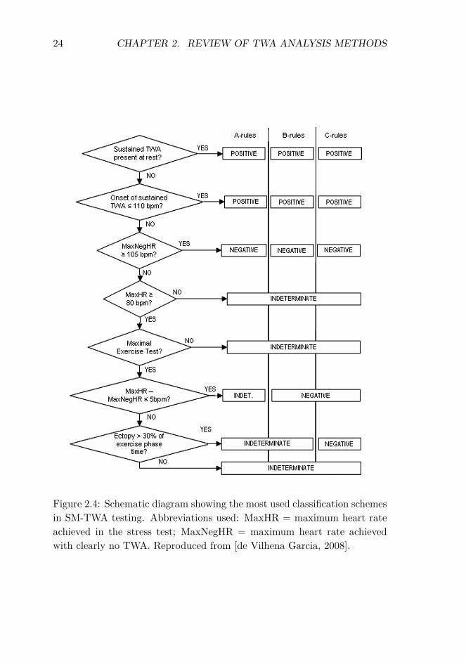
24 CHAPTER 2. REVIEW OF TWA ANALYSIS METHODS
A.N.E. � October 2008 � Vol. 13, No. 4 � Garcia � TWA Risk Stratification, Algorithms, and Limitations � 411
Figure 3. Schematic diagram showing the most used three-category classi-fication schemes in TWA testing with the SM technology. Most two-categoryschemes are based on grouping together positive and indeterminate tests inan “abnormal” cluster, though some may group only those indeterminate testswith specific indeterminacy causes. See text for information. Abbreviationsused: MaxHR = maximum heart rate achieved in the test; MaxNegHR: maxi-mum heart rate in the test with clearly no TWA. It is calculated backward, fromthe maximum heart rate to the basal heart rate.
difference between even-beat and odd-beat recur-sive (continuously updated) templates.70
Intrabeat Average
Intrabeat Average (IBA) concepts and featuresare much the same as those presented in the MMAapproach. Its hallmark is the splitting of the ST-Tcomplex in three time intervals (T-onset to T-peak—that includes ST segment; T-peak to T-end; T-onsetto T-end) and the computation of distinct TWA val-ues for each one of them.71–73
Adaptability to Clinical Settingsand Protocols
The selection of a TWA analysis algorithm forclinical (routine and research) purposes cannot relysolely on sensitivity, specificity, or predictive val-ues found in the scientific literature on the subject.That is because none of the most used methods hadits application reported in all the relevant clinicalsettings. SM—the most prolific method—has beenreported in the majority of studies on TWA in allclinical populations involved in TWA screening so
Figure 2.4: Schematic diagram showing the most used classification schemesin SM-TWA testing. Abbreviations used: MaxHR = maximum heart rateachieved in the stress test; MaxNegHR = maximum heart rate achievedwith clearly no TWA. Reproduced from [de Vilhena Garcia, 2008].
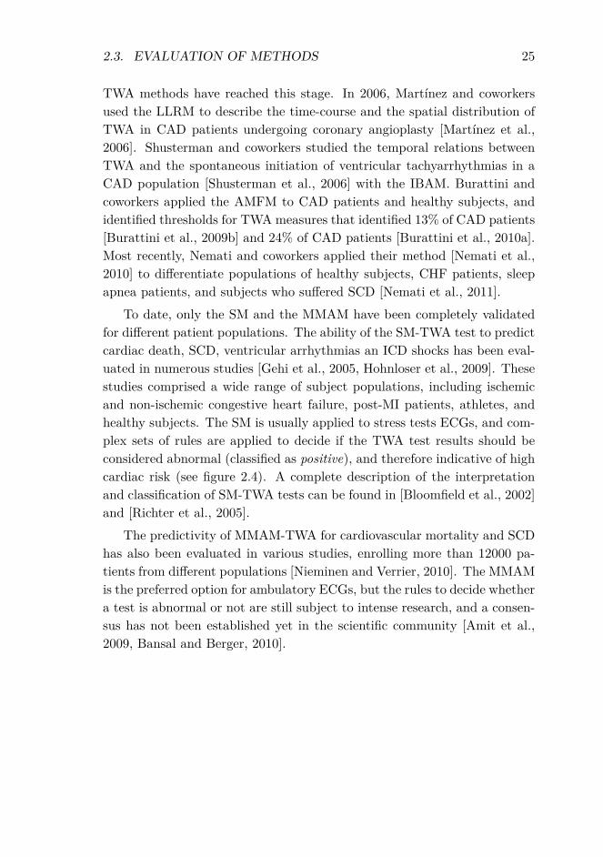
2.3. EVALUATION OF METHODS 25
TWA methods have reached this stage. In 2006, Martínez and coworkersused the LLRM to describe the time-course and the spatial distribution ofTWA in CAD patients undergoing coronary angioplasty [Martínez et al.,2006]. Shusterman and coworkers studied the temporal relations betweenTWA and the spontaneous initiation of ventricular tachyarrhythmias in aCAD population [Shusterman et al., 2006] with the IBAM. Burattini andcoworkers applied the AMFM to CAD patients and healthy subjects, andidentified thresholds for TWA measures that identified 13% of CAD patients[Burattini et al., 2009b] and 24% of CAD patients [Burattini et al., 2010a].Most recently, Nemati and coworkers applied their method [Nemati et al.,2010] to differentiate populations of healthy subjects, CHF patients, sleepapnea patients, and subjects who suffered SCD [Nemati et al., 2011].
To date, only the SM and the MMAM have been completely validatedfor different patient populations. The ability of the SM-TWA test to predictcardiac death, SCD, ventricular arrhythmias an ICD shocks has been eval-uated in numerous studies [Gehi et al., 2005, Hohnloser et al., 2009]. Thesestudies comprised a wide range of subject populations, including ischemicand non-ischemic congestive heart failure, post-MI patients, athletes, andhealthy subjects. The SM is usually applied to stress tests ECGs, and com-plex sets of rules are applied to decide if the TWA test results should beconsidered abnormal (classified as positive), and therefore indicative of highcardiac risk (see figure 2.4). A complete description of the interpretationand classification of SM-TWA tests can be found in [Bloomfield et al., 2002]and [Richter et al., 2005].
The predictivity of MMAM-TWA for cardiovascular mortality and SCDhas also been evaluated in various studies, enrolling more than 12000 pa-tients from different populations [Nieminen and Verrier, 2010]. The MMAMis the preferred option for ambulatory ECGs, but the rules to decide whethera test is abnormal or not are still subject to intense research, and a consen-sus has not been established yet in the scientific community [Amit et al.,2009, Bansal and Berger, 2010].

26 CHAPTER 2. REVIEW OF TWA ANALYSIS METHODS

Chapter 3
Common materials andmethods
3.1 Introduction
This chapter contains a unified description of the methods and materialsused throughout the thesis. It starts with the description of the basic single-lead analysis scheme that is usually followed by TWA methods, and detailstwo of those methods: the LLR and the SM. Then, the chapter presentsthe general multilead scheme proposed in this thesis, and discusses severaloptions to adapt the scheme to different analysis scenarios. The chapterends with a description of the ECG datasets used to validate the methods.
3.2 Basic scheme for single-lead analysis
According to the framework proposed by Martínez and Olmos [Martínezand Olmos, 2005], TWA analysis methods can be described using a generalscheme, such as the one in figure 3.1, consisting of three main processes:signal preprocessing, TWA detection, and estimation of TWA magnitudeand/or waveform. The preprocessing stage prepares the raw ECG signalfor TWA analysis, and then the stages of detection and estimation operateindividually on each ECG lead. These stages are described next.
27
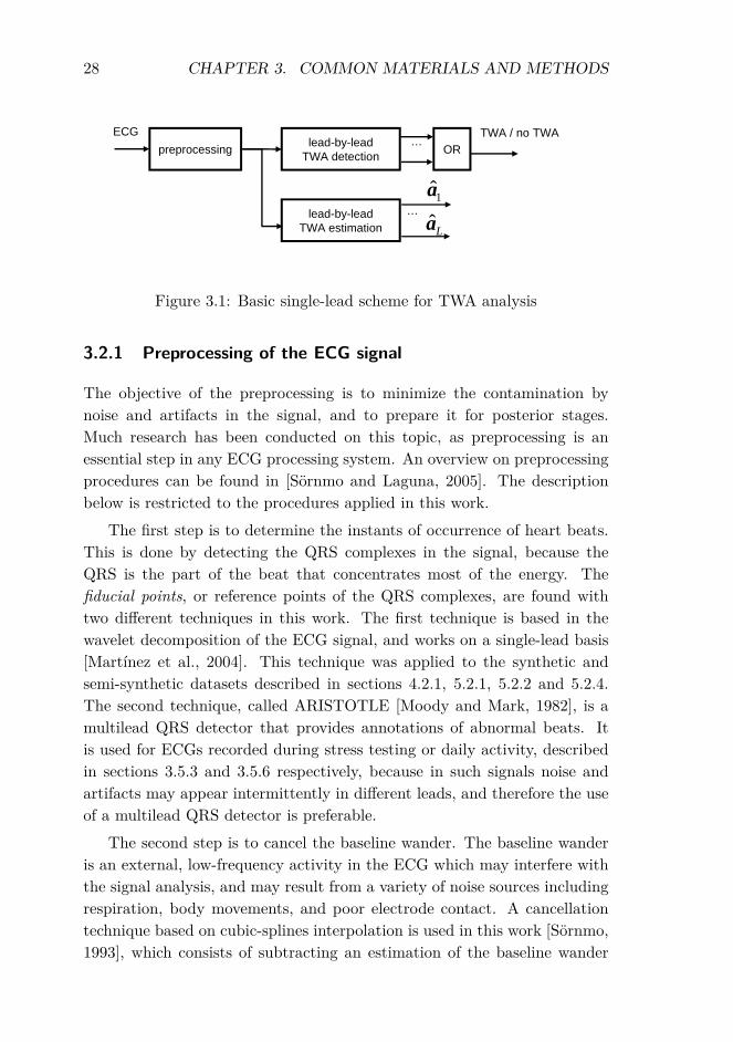
28 CHAPTER 3. COMMON MATERIALS AND METHODS
ECG…
preprocessing lead-by-leadTWA detection OR
ˆ
TWA / no TWA
…ˆLa
1alead-by-lead
TWA estimation
Figure 3.1: Basic single-lead scheme for TWA analysis
3.2.1 Preprocessing of the ECG signal
The objective of the preprocessing is to minimize the contamination bynoise and artifacts in the signal, and to prepare it for posterior stages.Much research has been conducted on this topic, as preprocessing is anessential step in any ECG processing system. An overview on preprocessingprocedures can be found in [Sörnmo and Laguna, 2005]. The descriptionbelow is restricted to the procedures applied in this work.
The first step is to determine the instants of occurrence of heart beats.This is done by detecting the QRS complexes in the signal, because theQRS is the part of the beat that concentrates most of the energy. Thefiducial points, or reference points of the QRS complexes, are found withtwo different techniques in this work. The first technique is based in thewavelet decomposition of the ECG signal, and works on a single-lead basis[Martínez et al., 2004]. This technique was applied to the synthetic andsemi-synthetic datasets described in sections 4.2.1, 5.2.1, 5.2.2 and 5.2.4.The second technique, called ARISTOTLE [Moody and Mark, 1982], is amultilead QRS detector that provides annotations of abnormal beats. Itis used for ECGs recorded during stress testing or daily activity, describedin sections 3.5.3 and 3.5.6 respectively, because in such signals noise andartifacts may appear intermittently in different leads, and therefore the useof a multilead QRS detector is preferable.
The second step is to cancel the baseline wander. The baseline wanderis an external, low-frequency activity in the ECG which may interfere withthe signal analysis, and may result from a variety of noise sources includingrespiration, body movements, and poor electrode contact. A cancellationtechnique based on cubic-splines interpolation is used in this work [Sörnmo,1993], which consists of subtracting an estimation of the baseline wander
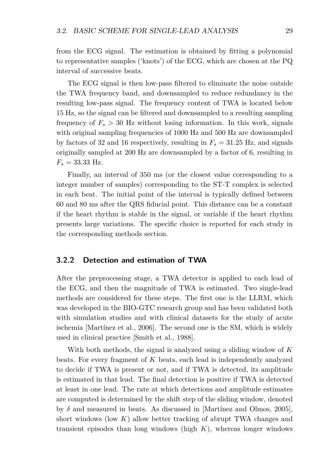
3.2. BASIC SCHEME FOR SINGLE-LEAD ANALYSIS 29
from the ECG signal. The estimation is obtained by fitting a polynomialto representative samples (‘knots’) of the ECG, which are chosen at the PQinterval of successive beats.
The ECG signal is then low-pass filtered to eliminate the noise outsidethe TWA frequency band, and downsampled to reduce redundancy in theresulting low-pass signal. The frequency content of TWA is located below15 Hz, so the signal can be filtered and downsampled to a resulting samplingfrequency of Fs > 30 Hz without losing information. In this work, signalswith original sampling frequencies of 1000 Hz and 500 Hz are downsampledby factors of 32 and 16 respectively, resulting in Fs = 31.25 Hz, and signalsoriginally sampled at 200 Hz are downsampled by a factor of 6, resulting inFs = 33.33 Hz.
Finally, an interval of 350 ms (or the closest value corresponding to ainteger number of samples) corresponding to the ST-T complex is selectedin each beat. The initial point of the interval is typically defined between60 and 80 ms after the QRS fiducial point. This distance can be a constantif the heart rhythm is stable in the signal, or variable if the heart rhythmpresents large variations. The specific choice is reported for each study inthe corresponding methods section.
3.2.2 Detection and estimation of TWA
After the preprocessing stage, a TWA detector is applied to each lead ofthe ECG, and then the magnitude of TWA is estimated. Two single-leadmethods are considered for these steps. The first one is the LLRM, whichwas developed in the BIO-GTC research group and has been validated bothwith simulation studies and with clinical datasets for the study of acuteischemia [Martínez et al., 2006]. The second one is the SM, which is widelyused in clinical practice [Smith et al., 1988].
With both methods, the signal is analyzed using a sliding window of Kbeats. For every fragment of K beats, each lead is independently analyzedto decide if TWA is present or not, and if TWA is detected, its amplitudeis estimated in that lead. The final detection is positive if TWA is detectedat least in one lead. The rate at which detections and amplitude estimatesare computed is determined by the shift step of the sliding window, denotedby δ and measured in beats. As discussed in [Martínez and Olmos, 2005],short windows (low K) allow better tracking of abrupt TWA changes andtransient episodes than long windows (high K), whereas longer windows

30 CHAPTER 3. COMMON MATERIALS AND METHODS
produce a greater smoothing on the beat-to-beat series under analysis, whichreduces the noise in the detection statistics and amplitude estimators. Inthis thesis, values of K ranging from 16 to 128 are considered, dependingon the noise characteristics of signals. The influence of the sliding step δ
was also discussed in [Martínez and Olmos, 2005]; a value of δ equal to onebeat allows a beat-to-beat sampling of the TWA evolution, whereas greatervalues such as δ = K/2 or δ = K provide less correlated measures, which canbe useful for the statistical characterization of the methods’ performance.The way LLRM and SM operate is summarized next.
Laplacian Likelihood Ratio method
The LLRM computes beat-to-beat the maximum likelihood estimation(MLE) of the TWA under the assumption of Laplacian noise, and applies ageneralized likelihood ratio test (GLRT) to decide whether TWA is presentor not.
Let K be the number of beats under analysis, N the number of samplesof each ST-T complex, and L the number of leads. The ST-T complex ofthe kth beat and the lth lead is represented with a row vector as
xk,l =[xk,l(0) . . . xk,l(N − 1)
]T. (3.1)
The LLR method assumes the following model for each complex
xk,l(n) = sl(n) + 12al(n)(−1)k + vk,l(n), n = 0 . . . N − 1 (3.2)
which in vector notation is
xk,l = sl + 12al(−1)k + vk,l (3.3)
where sl is the background ST-T complex, which is periodically repeatedin every beat, al is the TWA waveform, defined as the difference betweenodd and even beats, and vk,l is additive random noise (vectors in (3.3) aredefined as in (3.1)).
Background ST-T complexes can be canceled with a detrending filterthat computes the difference between each complex and the previous one
x′k,l = xk,l − xk−1,l, k = 1 . . . K − 1 (3.4)
The noise present in x′k,l is assumed to be independent and identically dis-tributed Laplacian with zero mean and unknown standard deviation σl. The

3.2. BASIC SCHEME FOR SINGLE-LEAD ANALYSIS 31
MLE of al for this model is given by [Martínez and Olmos, 2003, Martínezet al., 2006]
al(n) = median({x′k,l(n)(−1)k
}K−1
k=1
)n = 0 . . . N − 1 (3.5)
and the TWA amplitude is calculated as the root mean square (RMS) valueacross the estimated TWA waveform as
Valtl=
√√√√ 1N
N−1∑n=0
a2l (n) (µV ). (3.6)
The GLRT statistic can be expressed as
Zl =√
2σlNK
N−1∑n=0
(K−1∑k=1
∣∣∣x′k,l(n)∣∣∣− K−1∑
k=1
∣∣∣x′k,l(n)− al(n)(−1)k∣∣∣) (3.7)
where σl is the MLE of the standard deviation of the noise
σl =√
2NK
K−1∑k=1
∥∥∥x′k,l − al(−1)k∥∥∥
1. (3.8)
Details of the derivation of the MLE and GLRT are included in appendix3.A, and can also be found in [Martínez and Olmos, 2003, Martínez et al.,2006].
To decide whether TWA is present or not, the GLRT statistic Zl is com-pared to a threshold γ. TWA detection is positive if Zl > γ, and negativeotherwise. Since the detection statistic (3.7) is invariant to amplitude scal-ing of x′k,l (it is a constant false alarm rate (CFAR) detector), the value ofγ can be set to obtain a fixed probability of false alarm (PFA) regardless ofthe noise level [Kay, 1998].
Spectral Method
The SM [Smith et al., 1988, Rosenbaum et al., 1994] is based on Fourieranalysis of each beat-to-beat series of synchronized samples within the ST-Tcomplex. The TWA component is obtained by evaluating the Fast Fouriertransform (FFT) at the alternans frequency, which is 0.5 cycles per beat(cpb), or equivalently, 1 cycle every two beats. Following the notation in[Martínez and Olmos, 2005], the detection statistic can be expressed asZl = (1/N)
∑N−1n=0 zl(n) , where zl(n) = (1/K) |FFT {xk,l(n)}|2f=0.5 is the
0.5 cpb frequency bin of the short-time periodogram computed from the
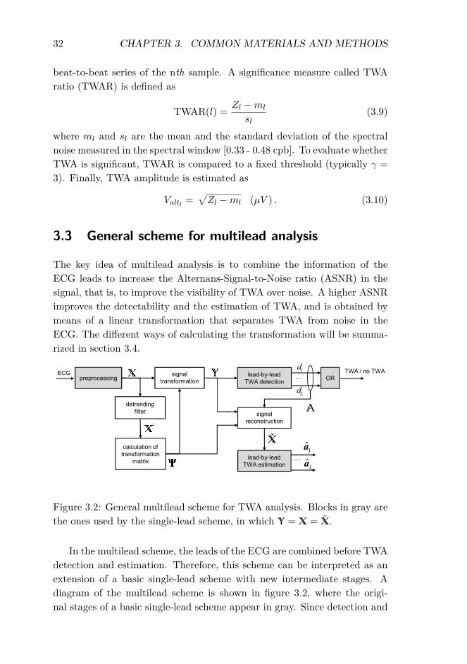
32 CHAPTER 3. COMMON MATERIALS AND METHODS
beat-to-beat series of the nth sample. A significance measure called TWAratio (TWAR) is defined as
TWAR(l) = Zl −ml
sl(3.9)
where ml and sl are the mean and the standard deviation of the spectralnoise measured in the spectral window [0.33 - 0.48 cpb]. To evaluate whetherTWA is significant, TWAR is compared to a fixed threshold (typically γ =3). Finally, TWA amplitude is estimated as
Valtl=√Zl −ml (µV ) . (3.10)
3.3 General scheme for multilead analysis
The key idea of multilead analysis is to combine the information of theECG leads to increase the Alternans-Signal-to-Noise ratio (ASNR) in thesignal, that is, to improve the visibility of TWA over noise. A higher ASNRimproves the detectability and the estimation of TWA, and is obtained bymeans of a linear transformation that separates TWA from noise in theECG. The different ways of calculating the transformation will be summa-rized in section 3.4.
ECG
…
…preprocessinglead-by-lead
TWA detection
signal
reconstruction
OR
Ld
1d
ˆLa
1a
lead-by-lead
TWA estimation
calculation of
transformation
matrix
detrending
filter
signal
transformation
TWA / no TWA
Figure 3.2: General multilead scheme for TWA analysis. Blocks in gray arethe ones used by the single-lead scheme, in which � = � = �.
In the multilead scheme, the leads of the ECG are combined before TWAdetection and estimation. Therefore, this scheme can be interpreted as anextension of a basic single-lead scheme with new intermediate stages. Adiagram of the multilead scheme is shown in figure 3.2, where the origi-nal stages of a basic single-lead scheme appear in gray. Since detection and

3.3. GENERAL SCHEME FOR MULTILEAD ANALYSIS 33
estimation stages do not change, it is possible to combine the extended mul-tilead scheme with any TWA analysis method that performs detection andestimation in separate stages. In particular, the multilead scheme can becombined with LLRM and SM just by computing the significance measures(GLRT or TWAR) and the amplitude estimates (eqs. (3.6) and (3.10)) inthe detection and the estimation stages respectively.
The stages of the general multilead scheme are summarized below. TheLLRM has been selected as the basic TWA analysis method for the descrip-tion, and an example of application to a synthetic signal with simulatedTWA has been included for illustration. The simulated signal belongs tothe synthetic dataset described in section 4.2.1 and is depicted in figure3.3(a).
3.3.1 Preprocessing of the ECG signal
The preprocesing stage consists of the same QRS detection, baseline cancel-lation, downsampling, and ST-T selection steps as the single-lead scheme.It was designed this way to facilitate the comparison of the analysis resultsobtained with the two schemes. As exactly the same preprocessing is ap-plied to the input signal, the preprocessing errors that may appear (QRSdetection errors, residual baseline wander, etc.) will equally affect the sin-gle and the multilead schemes, and therefore it will be correct to attributethe differences in the detection and estimation of TWA to the multileadtransformation of the signal.
At the end of the preprocessing stage, two multilead data matrices,� and �(m), are constructed as follows. Following the notation of thesingle-lead scheme, the ST-T complex of the kth beat and the lth lead isrepresented by the row vector
xk,l =[xk,l(0) . . . xk,l(N − 1)
]T.
For each lead l, ST-T segments are concatenated to form the (1×KN) leadvectors:
xl =[x0,l . . . xK−1,l
](3.11)
x(m)l =
[xm,l . . . xm+K−1,l
]where x(m)
l is the equivalent to xl obtained after sliding the analysis windowm beats forward. Two (L×KN) matrices are finally constructed by putting

34 CHAPTER 3. COMMON MATERIALS AND METHODS
together all the leads:
� =
x1...
xL
; �(m) =
x(m)
1...
x(m)L
(3.12)
where �(m) is a delayed version of �, and is necessary for one of the trans-formations described in section 3.4. For simplicity, it is omitted in figure3.2.
3.3.2 Signal transformation
The second stage aims to find a spatial transformation of the original leadsset that separates TWA from noise as much as possible. First, backgroundST-T segments are canceled with a detrending filter
x′k,l = xk,l − xk−1,l, k = 1 . . . K − 1 (3.13)
and the detrended beats x′k,l are arranged as in (3.11) and (3.12) to formmatrices �′ and �(m)′ . The application of the detrending filter is intendedto eliminate the background ECG, so that signals �′ and �(m)′ only con-tain a mixture of TWA and noise. This is necessary because otherwisethe separation techniques described later would tend to separate the back-ground ECG, not the TWA, from noise, since the background ECG hasgreater power than the TWA component. Then, the transformation Ψ iscalculated using a technique that separates TWA from the rest of the ECGcomponents.
Various techniques are employed to find the transformation matrix Ψin the thesis: PCA, πCA, Spectral Ratio Maximization (SRM), and In-dependent Component Analysis (ICA). These techniques are described insection 3.4. Once the transformation matrix is computed, it is applied tothe original data �
� = ΨT� (3.14)
to obtain the transformed signal �, whose leads (rows of �) will be denotedas transformed leads.
The objective of the linear transformation is to increase the separationbetween TWA and noise by projecting most of the TWA component ontoone subset of transformed leads, and most of the noise onto a differentsubset of leads. Therefore, TWA and noise will appear more separated in

3.3. GENERAL SCHEME FOR MULTILEAD ANALYSIS 35
the transformed signal than in the original signal, and the detection of TWAwill be easier. This effect is illustrated in figure 3.3(b), where TWA becomeseasily detectable in the transformed signal after PCA transformation.
3.3.3 Detection of TWA
The detection of TWA is performed exactly as in the single-lead scheme,but in this case the LLRM and SM operate on the transformed leads. Theresult of the lead-by-lead detection is denoted by dl: if TWA is detected inthe lth lead, then dl = 1, and dl = 0 otherwise. The final detection will bepositive if TWA is detected in one or more transformed leads (‘OR’ block infigure 3.2). In the example of figure 3.3(b), TWA is detected in transformedleads 5, 6, and 7 with the LLRM.
3.3.4 Signal reconstruction
Signal transformation can be interpreted as a change of coordinate sys-tem in the space. This means, for the example in figure 3.3(b), that thetransformed lead T1 does not correspond to the original lead V1. How-ever, clinicians use the amplitudes of TWA in the standard 12-lead systemor in the Frank lead system to decide about the results of clinical TWAtests. Therefore, in certain clinical scenarios it will be necessary to “re-verse” the transformation before estimating TWA. To solve this problem, areconstruction stage is included in the analysis scheme, where a new signalin the original lead set is reconstructed after TWA detection. In this way,TWA amplitude measurements can be computed in the original leads set,which also facilitates the comparison with the single-lead scheme.
To exactly reverse the transformation, we would need to do
� = (ΨT )−1� = Ψ�,
where the second equivalence holds true if Ψ is orthonormal. However, suchreconstruction would not improve the estimation of TWA over a single-lead scheme, since TWA would be estimated on the same original signal� as in the single-lead case. With the multilead scheme, the transformedleads where no TWA is detected are discarded first, and then a signal inthe original domain is reconstructed using only those transformed leadswith TWA. Discarding the transformed leads without TWA has a denoisingeffect that improves the estimation of TWA in the reconstructed signal, asthe following chapters will show.

36 CHAPTER 3. COMMON MATERIALS AND METHODS
� �
� � � �
��
��
�
�
��
��
��
��
��
�
�
� � � �
��
��
�
�
��
��
��
��
��
�
�
�
���
�
�
�
�
�
�
��
���
��
��
��
��
�
��
�
��
������������
��������
������ ���!�������
��������
��
��
� �
��
��
� �"� �"� �" �"�
��"�
��"�
��"�
��"�
��"�
� ��
��
��
��
�
��
�
��
���
��������
��������!� #$
� � � �
��
��
�
�
��
��
��
��
��
�
�
��
��
��
��
�
��
�
��
���
��������
��% �����%��!�������
Figure 3.3: (a) Simulated signal with TWA embedded in noise (ASNR= −20 dB). (b) Signal transformed with PCA. Asterisks indicate the trans-formed leads where TWA is detected (d5 = d6 = d7 = 1). (c) Reconstructedsignal. (d) Estimated TWA waveform.

3.3. GENERAL SCHEME FOR MULTILEAD ANALYSIS 37
Therefore, a diagonal matrix is defined from the lead-by-lead detectionas
� =
d1 0
. . .
0 dL
(3.15)
and the reconstruction matrix (ΨT )−1 is truncated as follows
ΨTR = (ΨT )−1�. (3.16)
Matrix ΨTR has zeros in columns corresponding to leads without TWA. Areconstructed signal is then obtained from the leads with detected TWA as
� = ΨTR�. (3.17)
The reconstructed data matrix � consists of the concatenation of the mul-tilead single-beat matrices Xk:
� =[X0 X1 . . . XK−1
](3.18)
whereXk =
[xk,1 . . . xk,L
]T(3.19)
with xk,l corresponding to the reconstructed ST-T complex of the kth beatin the lth lead. Note that � =
((ΨT )−1�ΨT
)� is equivalent to a spatially
filtered version of �, where the aim of the equivalent filter is to preservethe TWA content, not to obtain a perfect signal reconstruction. When nodetection is obtained, � = 0. Figure 3.3(c) shows the reconstructed signalfor the example case.
3.3.5 Estimation of TWA
Finally, TWA waveform and amplitude are estimated as in (3.5) and (3.6),but from the reconstructed signal � instead of from the original signal �.The estimated TWA for the example case is depicted in figure 3.3(d).
3.3.6 Variations of the general scheme
Throughout the thesis, several modifications of the general multilead schemeare considered, depending on the requirements of each particular study. Incases where the objective is to compare the detection power of different

38 CHAPTER 3. COMMON MATERIALS AND METHODS
ECG…preprocessing
lead-by-lead
TWA detectionOR
Ld
1d
calculation of
transformation
matrix
detrending
filter
signal
transformation
TWA / no TWA
Figure 3.4: Simplified multilead scheme for TWA detection.
ECG …preprocessing ˆ
La
1a
lead-by-lead
TWA estimation
calculation of
transformation
matrix
detrending
filter
signal
transformation
Figure 3.5: Modified multilead scheme for TWA analysis in situations whereno detection threshold can be determined.

3.4. SIGNAL TRANSFORMATION TECHNIQUES 39
alternatives, such as in studies reported in sections 4.4.3 and 5.4.3, a simpli-fied version of the general multilead scheme is used, in which reconstructionand estimation stages are omitted (figure 3.4).
For those cases where a detection threshold γ can not be set underrealistic assumptions, such as the clinical study with ambulatory records(see chapter 6), a modified version is proposed in which TWA is estimatedin the transformed leads (figure 3.5).
3.4 Signal transformation techniques
3.4.1 Principal Component Analysis
Principal component analysis (PCA) is a statistical technique which con-verts a set of correlated variables into a set of uncorrelated variables (“prin-cipal components”). In general, the objective of PCA is to condense theinformation of a large set of variables into a few variables, while main-taining the variability present in the dataset [Joliffe, 2002]. In this thesis,however, the main objective of PCA is to separate TWA from noise as muchas possible, since TWA and noise originate from different physical processes,and therefore it is sensible to assume that they are uncorrelated.
The derivation of principal components assumes that the signal �′ isa zero-mean random process with a spatial (inter-lead) correlation R
�′ =
E{�′�′T }. The principal components of �′ result from applying an or-thogonal linear transformation Ψ = [ψ1 ψ2 . . . ψL] to �′ ,
�′ = ΨT
�′, (3.20)
so that the rows of �′ (that is, the transformed leads) become mutuallyuncorrelated and sorted in descending order of variance. The first principalcomponent is obtained as a scalar product y′1 = ψT
1�′ , where the vector ψ1
is chosen so that the variance of y′1,
E{y′1y′T1 } = E{ψT
1�′�′Tψ1} = ψT
1 R�′ψ1 (3.21)
is maximized subject to the constraint that ψT1ψ1 = 1. The maximum
variance is obtained when ψ1 is chosen as the normalized eigenvector corre-sponding to the largest eigenvalue of R
�′ , denoted as λ1. In that case, the
resulting variance is
E{y′1y′T1 } = ψT
1 R�′ψ1 = λ1ψT1ψ1 = λ1. (3.22)

40 CHAPTER 3. COMMON MATERIALS AND METHODS
Subject to the constraint that y′1 and the second principal component y′2should be uncorrelated, y′2 is obtained by choosing ψ2 as the eigenvector cor-responding to the second largest eigenvalue of R
�′ , and so on. Accordingly,
to obtain the whole set of L different principal components, the eigenvectorequation for R
�′ needs to be solved,
R�′Ψ = ΨΛ (3.23)
where Λ denotes a diagonal matrix with the eigenvalues λ1 . . . λL sortedin descending order, and Ψ denotes the corresponding eigenvector matrix.Since R
�′ is unknown in practice, it can be approximated by the sample
correlation matrix, defined as
R�′ = 1
(K − 1)N�′�′T . (3.24)
Figure 3.3(b) shows the input signal in (a) after transformation with PCA.
3.4.2 Periodic Component Analysis
Periodic Component Analysis (πCA) is an eigenvalue technique for ana-lyzing periodic structure in multichannel signals. It was first proposed forspeech analysis [Saul and Allen, 2000] and then applied to the analysis ofECGs, for ECG compression and also for maternal and fetal ECG separation[Sameni et al., 2008].
This technique aims to find the projection y′ = wT�′ that maxi-
mizes the periodic structure of the signal at the TWA frequency, withw = [w1 w2 . . . wL]T being a column vector with L real weights. Todo so, a cost function is defined as
ε(w,m) =
∥∥∥y′(m) − y′∥∥∥2
∥∥∥y′∥∥∥2 (3.25)
where y′(m) = wT�′(m), with�′(m) defined in (3.12), andm = 2 beats is the
period of the TWA. This cost function is an inverse measure of periodicity:if the resulting signal y′ is periodic with period m, y′ = y′(m) and thereforeε(w,m) = 0.

3.4. SIGNAL TRANSFORMATION TECHNIQUES 41
Expanding the right hand side of (3.25) in terms of the weights w gives
ε(w,m) =
∥∥∥wT�′(m) −wT�
′∥∥∥2
‖wT�′‖2
=
∥∥∥wT (�′(m) −�′)∥∥∥2
‖wT�′‖2
= wT (�′(m) −�′)(�′(m) −�′)TwwT�
′�′TwT
=wT A
�′ (m)w
wT R�′w
where A�′ (m) is the spatial sample correlation of
(�(m)′ −�′
), and R
�′
is the spatial sample correlation of �′ , defined in (3.24).In the resulting expression,
ε(w,m) =wT A
�′ (m)w
wT R�′w
(3.26)
the numerator and denominator are both quadratic forms in the weights w.Such ratio is known as a Rayleigh quotient. By the Rayleigh-Ritz theoremof linear algebra, the weights w that minimize (3.26) are given by the gen-eralized eigenvector corresponding to the smallest generalized eigenvalue ofthe matrix pair
(A�′ (m), R
�′
)(see appendix 3.B for details).
Therefore, the transformation matrix Ψ is chosen as the generalizedeigenvector matrix of
(A�′ (m), R
�′
), with the eigenvectors (columns of
Ψ) sorted according to the corresponding eigenvalues in ascending order ofmagnitude. In this way, the transformation � = ΨT� projects the mostperiodic component into the first row of �, that is, TWA—if present—isprojected onto the first transformed lead, and therefore the first columnof Ψ can be interpreted as the spatial direction from which the periodiccontent of the signal is better observed.
3.4.3 Spectral Ratio Maximization
Spectral Ratio Maximization (SRM) is a novel technique proposed in thisthesis to improve the detection of TWA. Like πCA, SRM tries to find aprojection y′ = wT�
′ that maximizes the periodicity of the transformedsignal, but the measure of periodicity is now defined in the spectral domainas
ξ(w) = Sy(f0.5)∫Sy(f) df (3.27)
where Sy(f) is the power spectral density of the transformed signal, esti-mated with the modified periodogram, and f0.5 is the frequency of TWA(0.5 cycles per beat).

42 CHAPTER 3. COMMON MATERIALS AND METHODS
To find thew that maximizes (3.27), a gradient-based optimization algo-rithm is applied as implemented in MATLAB Optimization toolbox functionfminunc [Mat, 2002]. The algorithm follows a quasi-Newton approach anduses the Broyden-Fletcher-Goldfarb-Shanno (BFGS) method for updatingthe Hessian matrix (second partial derivatives of the objective function),which is widely believed to be the most effective technique for general use[Broyden, 1970, Fletcher, 1970, Goldfarb, 1970, Shanno, 1970]. Unlike PCAor πCA, in this case the transformed signal � will only contain one trans-formed lead.
To evaluate the sensitivity of the technique to the initial conditions,two options are considered to initialize the iterative algorithm: the vectorw = [1 0 . . . 0]T , which represents a projection on the first lead axis of theinput signal (SRM scheme), and the projection w obtained with πCA asdescribed above (πCA-SRM scheme).
3.4.4 Independent Component Analysis
Independent component analysis (ICA) is increasing in popularity in thefield of biomedical signal processing. It is generally used when it is requiredto separate measured biomedical signals into their constituent underlyingcomponents. Most applications of ICA are to multichannel time series mea-surements. In that case, the term blind source separation (BSS) can beused as a more generic identifier of the separation process [James and Hesse,2005].
The basic BSS problem that ICA attempts to solve assumes a set of Lobservations, in our case the matrix�′ defined in (3.12), to be a combinationof M unknown sources,
S =
s1...
sM
(3.28)
where the sources si are (1×KN) row vectors. The mixing of the sources isgenerally assumed to be linear, and the mixing matrix describing the linearcombination of the sources is given by the full-rank (L×M) matrix U suchthat
�′ = US. (3.29)
It is also generally assumed that the number of underlying sources is lessthan or equal to the number of measurement channels (M ≤ L). In ourcase, it will be assumed that M = L.

3.4. SIGNAL TRANSFORMATION TECHNIQUES 43
The task of ICA algorithms is to recover the original sources S from theobservations �′ , and this translates to that of finding a de-mixing matrixW such that
S = W�′ , (3.30)
where S are the resulting estimates of the underlying sources. To computethe de-mixing matrix, ICA algorithms assume that the resulting sourcesmust be mutually independent. Statistical independence is a stronger as-sumption that uncorrelatedness, and while statistically independent sourcesare always uncorrelated, the contrary does not necessarily happen. Thismeans that independent variables are uncorrelated and have no higher or-der correlations.
Besides uncorrelatedness, statistical independence is based on higherorder statistics (HOS). It is possible to obtain an estimate S of the sourcesS if the sources are non-Gaussian [Hyvärinen et al., 2001]. In practice, itis enough to make the estimates S as non-Gaussian as possible because,according to the central limit theorem, sums of independent non-Gaussianrandom variables are closer to Gaussian than the originals. In this way,looking for independent sources is equivalent to looking for non-Gaussiansources.
In this thesis, two widely referenced techniques for implementing ICAfollowing a HOS approach are used: FastICA and JADE. FastICA is one ofthe most referenced ICA techniques in the literature [Hyvärinen, 1999] andit is freely distributed in http://www.cis.hut.fi/projects/ica/fastica/ (Lastaccessed: April 2011). The FastICA algorithm finds the transformation thatmaximizes the independence of the components by minimizing their mutualinformation with a fixed point algorithm.
JADE is a widely used algorithm [Cardoso and Souloumiac, 1993]that finds the transformation that maximizes the independence of thesignal components by jointly diagonalizing fourth-order cumulant ten-sors. The JADE algorithm is publicly available in http://perso.telecom-paristech.fr/~cardoso/guidesepsou.html (Last accessed: April 2011).
For the multilead scheme, the transformation matrix Ψ is chosen as thede-mixing matrix obtained with FastICA or JADE algorithms.

44 CHAPTER 3. COMMON MATERIALS AND METHODS
3.5 ECG Databases
Various datasets, consisting of both real ECGs and synthetic signals, areused along the thesis for the evaluation of the methods described in previoussections. This section presents the ECG databases that are either analyzedin the evaluation studies, or used as a basis for the generation of syntheticsignals.
3.5.1 STAFF-III Database
The STAFF-III database contains the ECGs from 102 patients at theCharleston Area Medical Center in West Virginia. Nine standard leads(V1-V6, I, II, and III) were recorded using equipment by Siemens-ElemaAB (Solna, Sweden) and digitized at a sampling rate of 1 kHz.
ECGs were recorded while patients underwent percutaneous translumi-nal coronary angioplasty (PTCA), which is a procedure for opening dam-aged or obstructed coronary arteries that involves the inflation of a ballooninside the artery to open it up. This inflation produces acute ischemia in thecells of the myocardium, which can induce TWA. The STAFF-III databasewas used in [Martínez et al., 2006] to characterize the relation between TWAand acute ischemia.
In this thesis, real TWA episodes were extracted from STAFF-III signalsto create the evaluation datasets described in sections 4.2.1 and 5.2.2.
3.5.2 PTB Diagnostic ECG Database
The PTB Diagnostic ECG Database was compiled by the Na-tional Metrology Institute of Germany and is publicly available athttp://www.physionet.org/physiobank/database/ptbdb/. The databasecontains 549 ECGs collected from healthy volunteers and patients with dif-ferent heart diseases. Each ECG record includes the conventional 12 leads,together with the 3 Frank leads, and is digitized at a sampling rate of 1kHz.
In this thesis, records from healthy volunteers were used to recreaterealistic noise conditions in the synthetic signals described in section 4.2.1.

3.5. ECG DATABASES 45
3.5.3 Stress Test Database
This data set was compiled at the University Hospital Lozano Blesa ofZaragoza (Spain) [Bailón et al., 2003]. It contains 12-lead ECGs recordedduring treadmill exercise test following Bruce protocol, at 1 kHz samplingrate with an amplitude resolution of 0.6 µV. Records belong to three dif-ferent groups: 211 patients with a negative clinical and electrical exercisetest (non-ischemic group), 66 asymptomatic volunteers from the SpanishArmy who underwent the exercise test with negative results for coronaryartery disease (volunteer group), and 79 patients with significant stenosisin at least one major coronary artery as shown by coronary angiography(ischemic group).
In this thesis, records from volunteer and non-ischemic groups were usedto create the evaluation dataset described in section 5.2.2. Records fromvolunteer and ischemic groups were analyzed to evaluate the clinical utilityof the multilead schemes, as reported in sections 4.4.4 and 5.4.4.
3.5.4 Physionet TWA Database
The Physionet T-Wave alternans database is a publicly available re-source compiled for the PhysioNet/Computers in Cardiology Challenge 2008[Moody, 2008]. It contains one hundred real and synthetic ECG records,sampled at 500 Hz and with an approximate duration of two minutes. Thesynthetic subset of the database consists of thirty-two 12-lead ECGs con-taining artificial TWA in calibrated amounts. The remaining 68 records arereal signals from different databases, 56 of which belong to patients withknown cardiac risk factors. Synthetic records have 12 leads, and real recordshave 2, 3 or 12 leads.
In this thesis, the analysis of this database with the multilead schemesbased on PCA and πCA is reported in section 5.4.5 as an example of appli-cation to a publicly available dataset.
3.5.5 MIT-BIH Noise Stress Test Database
This database includes 12 half-hour ECG recordings and 3 half-hour record-ings of noise typical in ambulatory ECG recordings [Moody et al., 1984].The noise recordings were made using physically active volunteers and stan-dard ECG recorders, leads, and electrodes; the electrodes were placed onthe limbs in positions in which the subjects’ ECGs were not visible. The

46 CHAPTER 3. COMMON MATERIALS AND METHODS
three noise records were assembled from the recordings by selecting inter-vals that contained predominantly baseline wander (in record ‘bw’), muscleartifact (in record ‘ma’, with a spectrum which overlaps that of the ECG,but which extends to higher frequencies), and electrode motion artifact (inrecord ‘em’, usually the result of intermittent mechanical forces acting onthe electrodes).
In this thesis, noise records ‘bw’, ‘ma’ and ‘em’ were used to createsynthetic signals with realistic noise, as described in sections 4.2.1 and 5.2.1.
3.5.6 MUSIC database
This database contains ambulatory ECGs and clinical follow-up informationof more than 900 patients with symptomatic chronic heart failure (CHF),who were enrolled in the MUSIC (MUerte Súbita en Insuficiencia Cardiaca)study, a prospective, multicenter study designed to assess risk predictorsfor cardiovascular mortality in patients with CHF [Vázquez et al., 2009].Twenty-four-hour ECGs with the XYZ orthogonal leads and a samplingrate of 200 Hz were recorded using SpiderView recorders (ELA Medical,Sorin Group, Paris, France).
In this thesis, a total of 650 patients with sinus rhythm were consideredfor the clinical study presented in chapter 6.

3.5. ECG DATABASES 47
Appendix 3.A: GLRT and MLE derivation for the LLRM
The derivation of the GLRT and the MLE for the LLRM presented herehas been taken from [Martínez and Olmos, 2003, 2005] and [Martínez et al.,2006].
As explained in section 3.2.2, the LLRM assumes the following modelfor the observed signal
xk = s + 12a(−1)k + vk (3.31)
which is the same equation that (3.3), but where the lead index l has beenomitted for simplicity, since the LLRM is applied to each lead independently.After applying the detrending filter in (3.4), we obtain
x′k = xk − xk−1 = a(−1)k + (vk − vk−1) = a(−1)k + wk, (3.32)
where the TWA waveform, a, is deterministic but unknown, and the rest ofundesired components are grouped into the noise term wk = vk−vk−1. TheLLRM assumes that the noise samples in wk follow a zero-mean Laplaciandistribution with unknown standard deviation σ. In this model, both theTWA waveform a and the noise level σ are assumed to be stationary withinthe analysis window, but are allowed to change as the analysis window runsthrough the record, allowing adaptation to changes in signal and noise.
Departing from this model, the TWA detection problem can be ex-pressed as the hypothesis test
H0 : a = 0H1 : a , 0. (3.33)
A data matrix is created by putting together all the observations in theanalysis window,
X′ =[x′T1 , . . . ,x
′TK−1
], (3.34)
were each column contains one observation of the data (that is, the sam-ples corresponding to one detrended beat). We can express the likelihoodfunction for this data matrix as
p(X′ ;a, σ
)=( 1√
2σ
)KN
exp{−√
2σ
K−1∑k=1
∥∥∥x′k − a(−1)k∥∥∥
1
}. (3.35)
The GLRT is given by the likelihood ratio
LG =p(X′ ; a, σ1, H1
)p(X′ ; σ0, H0
) H1><H0
γ, (3.36)

48 CHAPTER 3. COMMON MATERIALS AND METHODS
where the unknown parameters a and σ are replaced by their MLE undereach hypothesis (a is the MLE of a under H1, and σ1 and σ0 are the MLEof σ under H1 and H0 respectively).
Under H1, the MLE of a must fulfill the condition
a = arg maxa p(X′ ;a, σ,H1
), (3.37)
and, since finding the maximum of the likelihood function is equivalent tofinding the minimum of
−ln p(X′ ;a, σ,H1
)= −ln
( 1√2σ
)KN
+√
2σ
K−1∑k=1
∥∥∥x′k − a(−1)k∥∥∥
1, (3.38)
the condition in (3.37) can be rewritten as
a = arg minaK−1∑k=1
∥∥∥x′k − a(−1)k∥∥∥
1. (3.39)
It can be shown [Kay, 1993] that this condition is accomplished when a isthe median of the demodulated series
a = median({
x′k(−1)k}K−1
k=1
)(3.40)
which is the vector-notation equivalent to the expression given in (3.5).Equaling to zero the partial derivatives of (3.35) with respect to σ under
both hypothesis, we obtain the MLEs
σ0 =√
2KN
K−1∑k=1
∥∥∥x′k∥∥∥1(3.41)
and
σ1 =√
2KN
K−1∑k=1
∥∥∥x′k − a(−1)k∥∥∥
1, (3.42)
which is the expression given in (3.8). Substituting the MLEs in (3.36), weget the GLRT
LG =(σ0σ1
)KN H1><H0
γ. (3.43)
Applying the monotonically increasing function f(x) = x(1/KN)− 1 to bothsides of (3.43) we get the equivalent test
Z =√
2σ1KN
N−1∑n=0
z(n)H1><H0
γ′, (3.44)

3.5. ECG DATABASES 49
where
z(n) =K−1∑k=1
∣∣x′k(n)∣∣− K−1∑
k=1
∣∣∣x′k(n)− a(n)(−1)k∣∣∣ (3.45)
and γ′ = γ(1/KN) − 1 is the new threshold. The combination of (3.44) and(3.45) results in the expression given in (3.7).

50 CHAPTER 3. COMMON MATERIALS AND METHODS
Appendix 3.B: Generalized eigenvalues and theRayleigh quotient
The generalized eigenvalues problem can be stated as follows: givenmatrices A,B ∈ Rn×n, find e ∈ Rn, λ ∈ R so that
Ae = λBe. (3.46)
If B is non-singular, the solutions can be obtained by solving the equivalent(standard) eigenvalue problem
B−1Ae = λe. (3.47)
Now let us assume that both A and B are symmetric and, in addition,B is also positive definite. The ratio
r(w) = wT AwwT Bw , (3.48)
which is known as Rayleigh quotient, is closely related to the generalizedeigenvalues problem stated above. Let us determine the extremum pointsof r(w), that is, the points w∗ satisfying ∇r(w∗) = 0. The gradient ∇r(w)is calculated as
∇r(w) = 2Aw(wT Bw)− 2(wT Aw)Bw(wT Bw)2 = 2Aw− 2r(w)Bw
wT Bw . (3.49)
Setting ∇r(w) to 0, we obtain,
Aw = r(w)Bw, (3.50)
which can be identified with (3.46). Thus, the extremum points w∗ (ex-tremum values r(w∗)) are obtained as the eigenvectors e of the correspond-ing generalized eigenproblem. A formal prove of this result (the Rayleigh-Ritz theorem) can be found in [Strang, 1988].

Chapter 4
Evaluation of the multileadscheme based onPrincipal Component Analysis
4.1 Introduction
ECG signals present a high spatial redundancy that can be exploited withtechniques based on the eigenanalysis of input data, such as PCA orKarhunen-Loève transform (KLT) [Castells et al., 2007]. These techniqueshave been applied to ECG data compression and noise reduction [Olmoset al., 1999, Acar and Köymen, 1999, Paul et al., 2000, Wei et al., 2001],characterization and diagnosis of ischemia [García et al., 1999, 2003], repo-larization heterogeneity [Pueyo et al., 2009, Okin et al., 2002, Acar et al.,1999], atrial fibrillation [Faes et al., 2001, Castells et al., 2005] and separa-tion of maternal and fetal ECG [Kanjilal and Palit, 1997].
This chapter describes the evaluation of the multilead scheme for TWAanalysis that combines PCA with the LLRM. As stated in chapter 2,methodological evaluation of a new technique (that is, the quantificationof its detection power and its estimation accuracy) is a desirable prior stepto clinical validation (which quantifies the adequateness of the TWA testas a risk stratifier). The performance of the proposed scheme is evaluatedby means of a simulation study, where the multilead scheme is comparedto the single-lead scheme which is the usual approach to TWA analysis.Besides, an example of application to real signals is provided, to show thatthe performance improvement observed in simulation can also be obtained
51

52 CHAPTER 4. MULTILEAD ANALYSIS BASED ON PCA
in real datasets.
4.2 Data sets
4.2.1 Simulated data
Biomedical signal processing techniques are usually evaluated on standarddatabases, where the output of the technique is compared to reference an-notations established by experts. However, the main problem in the case ofTWA analysis is the lack of validation databases, mainly because TWA isoften non-visible due to its low amplitude. Therefore, in this work a MonteCarlo simulation approach was adopted. To evaluate the multilead schemeand to compare it with the single-lead scheme, a simulation study was de-signed, where synthetic ECG signals were generated with a high degree ofrealism, and where TWA parameters (amplitude, waveform) were known apriori.
Multilead ECG signals were generated by adding noise and TWA to aclean background ECG (see figure 4.1). A standard beat from a 12-leadECG record was selected to create the background ECG. A TWA waveformwas detected and extracted from another 12-lead record using the LLRM.Both records belonged to the STAFF-III database (see section 3.5.1). Fromthe 12-lead set, only the eight independent leads were selected (L = 8).
Four types of noise were considered: Gaussian (gs), Laplacian (lp), elec-trode motion (em) and muscular activity (ma). Noise types gs and lp wererandomly generated. Types em and ma, which are typical noises present inthe ECG, were extracted from two real noise records of the MIT-BIH NoiseStress Test Database (see section 3.5.1).
Each Monte Carlo trial was generated as the sum of the backgroundECG beat repeated K times, the TWA waveform repeated K times withalternating sign, and a random realization of noise. Each realization ofnoise was generated as follows. First, L segments of KN samples weresimulated (gs or lp noise) or extracted from the records beginning at arandom position (em or ma noise). Baseline wander was removed from em
andma noises, because em andma records contain low frequency variationsof high amplitude that can distort the level of noise actually added to thesimulated ECG. Noise segments were normalized to a 1 µV RMS value and

4.2. DATA SETS 53
Figure 4.1: Simulation of multilead ECG signals with TWA and noise. Sig-nals scale is not preserved for better visualization.
piled to form a multilead matrix V
V =[v1 . . . vL
]T(4.1)
Due to the noise generation setup, noise segments vl are spatially uncor-related (RV = �). However, noise in real signals is spatially correlated.To correlate V in a realistic way, the first step was to estimate the spatialcorrelation of real ECG noise using 10 multilead ECG records of the PTBDiagnostic ECG database (see section 3.5.2). Figure 4.2 illustrates the pro-cess followed to estimate the correlation. A total of 2000 segments of noisewere selected from each independent lead by taking the 50 ms interval priorto a P wave onset for each segment, since that interval is assumed to beisoelectric. DC level was removed, and segments corresponding to each leadwere concatenated. The resulting noise leads were piled as in (4.1) to forma noise matrix N. The spatial correlation of N was estimated as
RN = 1M
NNT (4.2)
where M is the number of samples of each noise lead. The Cholesky de-composition [Golub and Van Loan, 1989] was applied to the inverse of the

54 CHAPTER 4. MULTILEAD ANALYSIS BASED ON PCA
noise correlation matrix to obtain a whitening matrix D
R−1N = DTD (4.3)
whereD is an upper triangular matrix with strictly positive diagonal entries.The inverse of D was used to spatially correlate the generated noise V
V′ = D−1V (4.4)
thus obtaining a correlated noise matrixV′ with a spatial correlationRV′ =RN , that is,
RV′ = E{V′V′T
}= D−1E
{VVT
}(D−1)T = D−1(D−1)T = RN . (4.5)
Finally, the correlated noise V′ was scaled so that the RMS value of theleast noisy lead was Vnoise = 200 µV . TWA was then scaled to obtain adesired Alternans-Signal-to-Noise ratio (ASNR), defined as the maximumratio between TWA power and noise power in the L leads:
ASNR = 10 log(Valt/2)2
V 2noise
(4.6)
where Valt is the maximum RMS value of the TWA waveforms in the L leads,that is, Valt = max{Valt1 . . . ValtL
}, with Valtldefined in (3.6). Multilead
ECG signals were simulated with ASNR levels ranging from -60 to 10 dB,and also without TWA. For each type of noise, a total of 104 realizations ofnoise were generated to simulate signals without TWA, and 104 realizationsfor each ASNR level to generate signals with TWA.
4.2.2 Stress test signals
As an example of application to real data, TWA analysis was performed onthe set of stress test ECG records presented in section 3.5.3. Records fromvolunteer and ischemic groups were selected for TWA analysis. Volunteerrecords had an average duration of 20 min, and the maximum heart rate(HR) over the test was 183 ± 8 beats per minute (bpm) (mean ± standarddeviation). Ischemic records had an average duration of 16 min, and themaximum heart rate over the test was 134 ± 23 bpm.
4.3 Methods for TWA analysis
The complete simulated dataset was processed with the LLRM, follow-ing the basic single-lead scheme (see figure 3.1) and the general multilead

4.4. RESULTS 55
noise correlation
50 ms
DC eliminationand
concatenation
0
0
0
0
0
0
0
0
0
0
0
Figure 4.2: Illustration of the estimation of noise spatial correlation RN inreal ECGs.
scheme (see figure 3.2), with an analysis window of K = 32 beats and δ =1 beat. Besides, simulated signals with ma noise were processed with bothLLRM and SM, following the single-lead scheme and the simplified multi-lead scheme (see figure 3.4). For the comparison between LLRM and SM,a 128-beat analysis window was selected, since that is the window lengthused in commercial SM systems. In all cases the initial point of the ST-Tcomplex was set 60 ms after the QRS fiducial point.
Stress test records were processed with the LLRM, following the single-lead scheme and the general multilead scheme, with a 128-beat analysiswindow and δ = 1 beat. The initial points of ST-T complexes were set 80ms after the QRS fiducial point if the mean HR in the analysis window was≤ 100 bpm, and 60 ms after the QRS fiducial point if the mean HR was >100 bpm.
4.4 Results
4.4.1 Detection performance
Following the terminology of detection theory [Kay, 1998], probability offalse alarm (PFA) was defined as the ratio between the number of positiveTWA detections in signals with Valt = 0 (false detections) and the total

56 CHAPTER 4. MULTILEAD ANALYSIS BASED ON PCA
0.8
1single-lead schememultilead scheme
emgslp mama
ASNR = -25 dB
0.8
1
0.4
0.6 lp
gs0.4
0.6
P D P D
0 0.2 0.4 0.6 0.8 1P
FA
0 0.2 0.4 0.6 0.8 10
0.2
PFA
em
0
0.2
0.8
1
0.8
1single-lead schememultilead scheme
ASNR = -35 dB
emgslp ma
0.4
0.6
P D
0.4
0.6 em
gs
lp
ma
P D
0 0.2 0.4 0.6 0.8 10
0.2
0 0.2 0.4 0.6 0.8 10
0.2
PFA
PFA
Figure 4.3: ROC curves for ASNR = −25 dB (corresponding to Valt = 22.5µV) and ASNR = −35 dB (Valt = 7.1 µV) of the multilead scheme (left)and the single-lead scheme (right) combined with LLRM for Gaussian (gs),Laplacian (lp), muscular activity noise (ma) and electrode movement noise(em).

4.4. RESULTS 57
0.8
1
0.8
1single-lead schememultilead scheme
gslp
ma
ASNR = -45 dB
0.4
0.6
PD
0.4
0.6
PD
em
em
lp
gs
0 0.2 0.4 0.6 0.8 10
0.2
PFA
0 0.2 0.4 0.6 0.8 10
0.2
PFA
em
ma
0.8
1
0.8
1single-lead schememultilead scheme
ma
ASNR = -50 dB
0.4
0.6
0.4
0.6em
gs
lp
em
lp
gs
PD
PD
PFA PFA
0 0.2 0.4 0.6 0.8 10
0.2
0 0.2 0.4 0.6 0.8 10
0.2
em
ma
Figure 4.4: ROC curves for ASNR = −45 dB (corresponding to Valt = 2.2µV) and ASNR = −50 dB (Valt = 1.3 µV) of the multilead scheme (left)and the single-lead scheme (right) combined with LLRM for Gaussian (gs),Laplacian (lp), muscular activity noise (ma) and electrode movement noise(em).
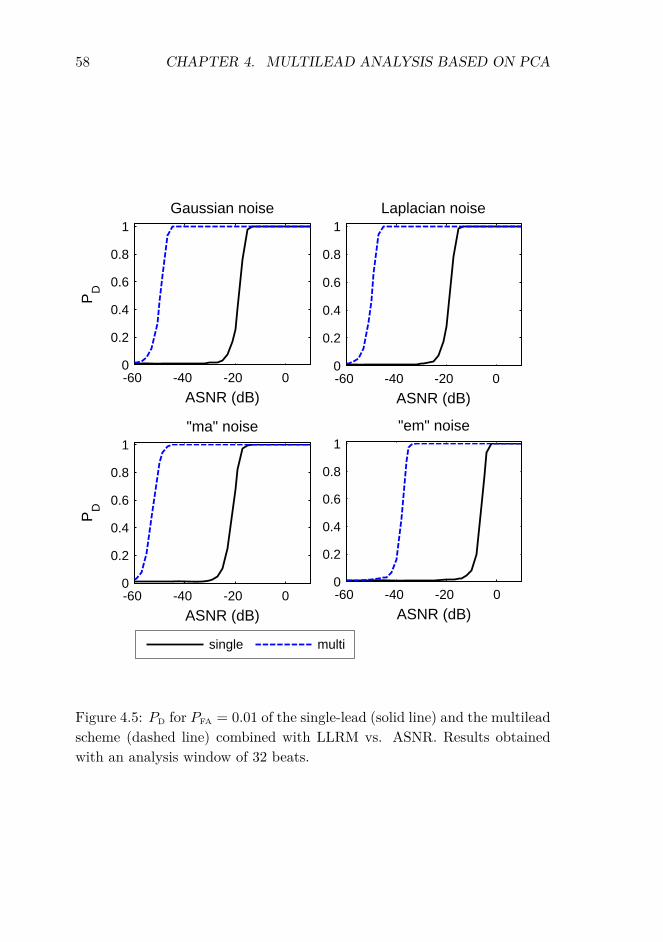
58 CHAPTER 4. MULTILEAD ANALYSIS BASED ON PCA
-60 -40 -20 00
0.2
0.4
0.6
0.8
1Gaussian noise
ASNR (dB)
PD
-60 -40 -20 00
0.2
0.4
0.6
0.8
1Laplacian noise
ASNR (dB)
-60 -40 -20 00
0.2
0.4
0.6
0.8
1"ma" noise
ASNR (dB)
PD
-60 -40 -20 00
0.2
0.4
0.6
0.8
1"em" noise
ASNR (dB)
single multi
Figure 4.5: PD for PFA = 0.01 of the single-lead (solid line) and the multileadscheme (dashed line) combined with LLRM vs. ASNR. Results obtainedwith an analysis window of 32 beats.

4.4. RESULTS 59
number of decisions made in those signals. Probability of detection (PD)was defined as the ratio between the number of positive TWA detections insignals with a given Valt and the total number of decisions made in thosesignals. Detection performance was evaluated with receiver operating char-acteristic (ROC) curves, which show the relationship between PD and PFA
as a function of the detection threshold γ. Figure 4.3 shows the ROC curvescorresponding to ASNR = −25 dB and −35 dB. Figure 4.4 shows the ROCcurves corresponding to ASNR = −45 dB and −50 dB. For every typeof noise and ASNR level, the area under the ROC curve of the multileadscheme was greater than the area under the single-lead curve.
To better analyze the behavior of the schemes for different ASNR levels,a fixed value for γ was selected so that PFA= 0.01, and the resulting PD wascompared. Detection thresholds were set to γ = 0.06 for gs noise, γ = 0.06for lp noise, γ = 0.06 for ma noise, and γ = 0.162 for em noise. Figure 4.5shows the PD of the two schemes vs. ASNR for all types of noise. In allcases, the multilead scheme outperforms the single-lead scheme. The ASNRlevel where PD achieves a value of 0.99 is 30 dB lower with the multileadscheme than with the single-lead scheme for gs and lp noises, 28 dB lowerfor em noise, and 27 dB lower for ma noise.
4.4.2 Estimation accuracy
The estimation performance of the two schemes was evaluated in terms ofbias, variance and mean square error. Let us denote by al (n) the nth sampleof the estimated TWA waveform in the lth lead, and by al (n) the samesample of the true TWA waveform. For each ASNR level, the expected valueof the estimation, E {al (n)}, and the standard deviation of its samples,σal
(n), were estimated as the samples average and the samples standarddeviation of al (n) in the 104 realizations respectively. The bias and meansquare error of the estimation were calculated for each lead l as
bl(n) = E {al(n)} − al(n), n = 0 . . . N − 1 (4.7)
e2l (n) = E
{(al(n)− al(n))2
}, n = 0 . . . N − 1 (4.8)
where the expected values were estimated as the average of the 104 realiza-tions. As explained in section 3.3.4, the reconstructed signal is � = 0 if noTWA is detected, and in that case al(n) = 0, n = 0 . . . N − 1.

60 CHAPTER 4. MULTILEAD ANALYSIS BASED ON PCA
Figures 4.6 and 4.7 show the expected value and the standard deviationof the estimation for gs noise and various levels of ASNR. For high levelsof ASNR (figure 4.6), the bias of the multilead estimation is higher thanthe bias of the single-lead estimation, but the standard deviation of themultilead estimation is lower. For low levels of ASNR (figure 4.7), bothbias and variance are lower for the multilead estimation.
To globally quantify the accuracy of the estimation at each ASNR level,two global performance parameters, Rbl
and Rel, were defined as
Rbl(%) =
√√√√ 1N
N−1∑n=0
b2l (n)√√√√ 1
N
N−1∑n=0
a2l (n)
× 100 (4.9)
Rel(%) =
√√√√ 1N
N−1∑n=0
e2l (n)√√√√ 1
N
N−1∑n=0
a2l (n)
× 100. (4.10)
Parameter Rblmeasures the relative bias of the estimation in the lth lead,
and parameter Relmeasures the relative error caused by both the bias and
the variance of the estimation. Figures 4.8 and 4.9 show the evolution ofRbl
and Relvs. ASNR for ma noise. For ASNR ≥ −15 dB, the bias of the
multilead estimation is higher than the bias of the single-lead estimation.For ASNR < −25 dB, the bias of the single-lead estimation tends to 100%for all the leads. Rb and Re curves for gs, lp, and em noises are included inappendix 4.A. The same trend appears with all noise types: for high ASNRlevels, Rel
is similar for both schemes, and for low ASNR levels it is lowerfor the multilead scheme.
4.4.3 Comparison with the Spectral Method
As explained in the methods section, simulated signals with ma noise wereprocessed with the single-lead and multilead schemes combined with LLRM(LLR single and LLR multi respectively), and also with the two schemescombined with SM (SM single and SM multi).
To ensure a fair comparison, detection thresholds were set so that theresulting PFA was 0.01 for every technique (table 4.1). Detection curves for

4.4. RESULTS 61
-3
--2
-1
0
-3
-2
-1
0
ASNR = 10 dBsingle-lead scheme multilead scheme
V1V2
V3
-8
-7
-6
-5
-4
-8
-7
-6
-5
-4V4
V5
V6I
II
mV
0 0.1 0.2 0.3 0 0.1 0.2 0.3
(a) (b)
II
time (s) time (s)
0
single-lead schemeASNR = -15 dB
0
multilead schemeV1
-0.6
-0.4
-0.2
mV
-0.6
-0.4
-0.2V2
V3
V4
V5
0 0.1 0.2 0.3
-1.0
-0.8
(c)time (s)
0 0.1 0.2 0.3
-1.0
-0.8
(d)
V5
V6
I
II
time (s)
Figure 4.6: Expected value E {al (n)} (solid line) and standard deviationσal
(n) (vertical bars) of the TWA waveforms estimated with the LLRM,obtained with (a) the single-lead and (b) the multilead scheme for ASNR =10 dB, and with (c) the single-lead and (d) the multilead scheme for ASNR= -15 dB for gs noise. The true TWA is shown in dashed line. Leads offsetis included for better visualization.

62 CHAPTER 4. MULTILEAD ANALYSIS BASED ON PCA
60
-40
-20
0
20
-40
-20
0
20
ASNR = -30 dBsingle-lead scheme multilead scheme
V1
V2
V3
-160
-140
-120
-100
-80
-60
-160
-140
-120
-100
-80
-60
V4
V5
V6III
mV
0
0 0.1 0.2 0.3-180
0 0.1 0.2 0.3-180
(a) (b)time (s) time (s)
single-lead schemeASNR = -40 dB
multilead scheme
V1
-60
-40
-20
0
-60
-40
-20
0
mV
V1
V2
V3
V4
V5
V6
0 0.1 0.2 0.3
-100
-80
0 0.1 0.2 0.3
-100
-80
(c)time (s)
(d)
V6
I
II
time (s)
Figure 4.7: Expected value E {al (n)} (solid line) and standard deviationσal
(n) (vertical bars) of the TWA waveforms estimated with the LLRM,obtained with (a) the single-lead and (b) the multilead scheme for ASNR= -30 dB, and with (c) the single-lead and (d) the multilead scheme forASNR = -40 dB for gs noise. True TWA shown in dashed line. Leads offsetincluded for better visualization.
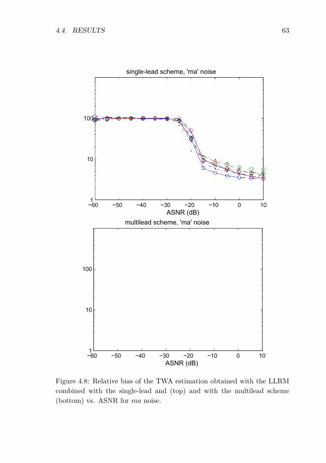
4.4. RESULTS 63
Figure 4.8: Relative bias of the TWA estimation obtained with the LLRMcombined with the single-lead and (top) and with the multilead scheme(bottom) vs. ASNR for ma noise.

64 CHAPTER 4. MULTILEAD ANALYSIS BASED ON PCA
Figure 4.9: Relative error of the TWA estimation obtained with the LLRMcombined with the single-lead and (top) and with the multilead scheme(bottom) vs. ASNR for ma noise.

4.4. RESULTS 65
single-lead multileadLLRM 0.03 0.01
SM 9.47 5.95
Table 4.1: Detection thresholds which are necessary to obtain a PFA = 0.01in the simulated dataset with ma noise, using the different schemes and a128-beat analysis window.
all techniques are shown in figure 4.10. The best results are obtained withthe LLR multi technique. The ASNR level where PD achieves a value of0.99 is 8 dB lower for LLR single than for SM single, 6 dB lower for LLRmulti than for SM multi, 30 dB lower for SM multi than for SM single, and28 dB lower for LLR multi than for LLR single.
LLR single
SM singleSM multi
LLR multi
Figure 4.10: PD vs. ASNR for the single lead scheme combined with LLRM(LLR single) and with SM (SM single), and for the multilead scheme com-bined with LLRM (LLR multi) and with SM (SM multi). PFA = 0.01 in allcases. Results obtained with an analysis window of 128 beats.
4.4.4 Application to stress test signals
TWA is a phenomenon partially related to heart rate, so TWA arises inpatients at risk for SCD but also in healthy subjects at faster heart ratesduring stress tests. Therefore, the assumption that no TWA should be foundin volunteer records at heart rates below a cut-off heart rate HRc was madeto set the same PFA = 0.01 for both analysis schemes. Volunteer’s signals

66 CHAPTER 4. MULTILEAD ANALYSIS BASED ON PCA
HRc = 100 HRc = 110single-lead scheme 0.09 0.10multilead scheme 0.07 0.08
Table 4.2: Detection thresholds which are necessary to obtain a PFA = 0.01in volunteer records at heart rates below a cut-off heart rate HRc.
were processed, and for each scheme a threshold was calculated so that itwas exceeded only by 1% of the Z values obtained before heart rate reachedthe HRc, which were considered as false detections. Then, all records fromboth groups were processed with the resulting thresholds (table 4.2).
Table 4.3 contains the results obtained considering HRc = 110 bpm toset the PFA. The first row presents the total number of records of each group,and the number of records where one or more TWA episodes were detected.An episode was defined as an interval of consecutive beats in which TWAwascontinuously detected. For each episode, three parameters were calculated:the maximum TWA amplitude in the episode Vmax (µV ), the duration (inseconds), and the onset heart rate HRo (bpm), which was calculated as themean heart rate of the analysis window in which the episode begins. Foreach group, the mean value and the standard deviation of these parameterswere calculated in two ways: considering all the episodes (second row), andconsidering the episodes detected exclusively by one scheme and not bythe other (third row). Table 4.4 shows the number of records where TWAepisodes were detected before 110 bpm (PFA set with a HRc = 110 bpm),and the number of records where TWA episodes were detected before 100bpm (PFA = 0.01 set with a HRc = 100 bpm).
Differences in the number of records with TWA were evaluated withthe Fisher’s exact test; differences in mean values of Vmax, duration andHRo were evaluated with the Mann-Whitney U test. A p-value < 0.05 wasconsidered significant.
As an illustrative example, figures 4.11, 4.12 and 4.13 show how theschemes work with a signal belonging to the ischemic group (Sig1). Figure4.11 shows the detection statistic Z obtained with the two schemes. Themaximum value of Z for the multilead scheme appears at instant tmax = 24minutes. At that time, the maximum Z with the single-lead scheme is ob-tained in lead V3, and with the multilead scheme in T6. Figure 4.12 showsthe superposition of even and odd beats in those leads. Figure 4.13 showsthe estimated TWA waveform in Sig1 at tmax. For illustration purposes,

4.5. DISCUSSION 67
the same detection threshold was chosen for both schemes, γ = 0.1, corre-sponding to the threshold obtained for the single-lead scheme in volunteerrecords with HRc = 110 bps (table 4.2). TWA was detected only by themultilead scheme, in the transformed lead T6.
4.5 Discussion
According to simulation results, the high detection performance of the mul-tilead scheme is similar for gs, lp and ma noises, (Figs. 4.3 and 4.4). It isworse when facing em noise, because the em bandwidth mostly overlaps theband of the TWA. Even in this case, the multilead scheme performs betterthan the single-lead scheme. Note that in figures 4.3 and 4.4 the single-leadscheme is not capable of detecting anything for ASNR ≤ −35 dB in anytype of noise.
As shown in figure 4.5, the multilead scheme surpasses widely the per-formance of the single-lead scheme, detecting TWA with an ASNR from 27to 30 dB lower than the single-lead scheme for a fixed PD. The multileadscheme performs better, specially at low ASNR levels, because it separatesTWA from most of the noise. For instance, in figure 3.3(c) we can see that,at ASNR = −20 dB, noise is mainly concentrated in leads T1 - T3, so TWAbecomes detectable in leads T5 - T7.
In the example signal Sig1, the values of the detection statistic Z arehigher with the multilead scheme than with the single-lead scheme (figure4.11). Since the GLRT detector is CFAR, a higher PD can be obtainedfor a fixed threshold, or a lower number of false detections for a given PD.The main effect of PCA in this case is concentrating the noise in the firsttransformed leads, making TWA detectable in lead T6 (note that TWA isclearly visible in T6, but not in V3 in figure 4.12). With real signals, PCAwill work differently depending on the spatial autocorrelation of noise andTWA, and the cross-correlation between them. It may concentrate mainlythe noise, the TWA, or both. In the worst situation, when the correlationsof noise and TWA are similar, they won’t be separated at all. In that casethe multilead scheme will not improve the analysis, but it will not make theresult worse either.
Since the improvement obtained with the multilead scheme is mainlydue to the effect of PCA, similar detection gains can be expected whencombining the multilead scheme with other TWA techniques. For example,

68 CHAPTER 4. MULTILEAD ANALYSIS BASED ON PCA
multilead scheme single-lead schemevolunteer ischemic volunteer ischemic
Detectionrecords 66 70 66 70
records with TWA 26 27 19 20% records with TWA 39.4 38.6 28.8 28.6
TWA characteristicsall episodes Vmax (µV ) 85±114‡ 95±128 133±133‡ 135±146detected duration (s) 26±26 48±59 29±24 51±39by each HRo (bpm) 124±30† 106±20† 121±30† 105±20†
scheme episodes 38 33 26 22episodes Vmax (µV ) 21±15†‡ 37±22† 52±35‡ 66±35detected by one duration (s) 7±7 30±71 17±16 18±21scheme and not HRo (bpm) 127±27† 107±19† 112±7 105±18by the other episodes 17 18 5 7
Table 4.3: Results of TWA analysis in stress test data, calculated consid-ering all episodes regardless of when they are detected. (PFA = 0.01 forthe two schemes). Data expressed as (mean ± one standard deviation). †
indicates a significant difference between volunteer and ischemic groups; ‡
indicates a significant difference between multilead and single-lead schemes.
multilead scheme single-lead schemevolunteer ischemic volunteer ischemic
HRo < 110 bpmrecords 66 70 66 70
records with TWA 6† 14† 6 12% records with TWA 9.1† 20.0† 9.1 17.1
HRo < 100 bpmrecords 66 70 66 70
records with TWA 6† 14† 5 10% records with TWA 9.1† 20.0† 7.5 14.2
Table 4.4: Results of number of records with TWA in stress test data,calculated considering the episodes detected before heart rate reaches 110bpm (first row) and 100 bpm (second row). PFA = 0.01 for the two schemes.† indicates a significant difference in the number of records with TWA involunteer and ischemic groups.

4.5. DISCUSSION 69
0 10 200
0.05
0.1
0.15
0.2
GLR
T st
atis
tic (Z
)
single-lead scheme
time (min)0 10 20
0
0.05
0.1
0.15
0.2multilead scheme
time (min)
Figure 4.11: Detection statistic Z of LLRM computed with a 128-beatwindow in signal Sig1. Left panel: Z obtained with the single-lead schemein leads V1-V6, I and II after the preprocessing stage. Right panel: Z
obtained with the multilead scheme in transformed leads T1 -T8 after PCAtransformation. Threshold γ = 0.1 is shown in dashed line.

70 CHAPTER 4. MULTILEAD ANALYSIS BASED ON PCA
Figure 4.12: Superposition of odd (black) and even (gray) beats of a 128-beat analysis window centered on instant tmax = 24 min in signal Sig1.Top panel: beats of lead V3 (left), which is the lead where the maximumZ appears with the single-lead scheme, and a closer view of the ST-T com-plexes (right). Bottom panel: same views for lead T6, where the maximumZ appears with the multilead scheme. In this case, the morphology of theST-T complex is consistently different in odd and even beats, making TWAvisible to the naked eye.

4.5. DISCUSSION 71
100 200 300-10
-5
0
5
10
single-lead scheme
V
time (ms)100 200 300
-10
-5
0
5
10
multilead scheme
time (ms)
Figure 4.13: TWA waveform estimated in Sig1 at tmax = 24 min with thesingle-lead scheme (left), and the multilead scheme with γ = 0.1 (right).
in simulated data with ma noise, applying the multilead scheme to the SMyields an improvement of 30 dB over the single-lead approach, which issimilar to the improvement obtained by applying the multilead scheme tothe LLRM (28 dB) (see figure 4.10).
In the comparison of SM and LLRM, it is interesting to note that thederived threshold for the SM single scheme (γ = 9.47) is much higher thanthe usual SM significance threshold (TWAR = 3). In fact, the applicationof the SM single scheme with an equivalent γ = 3 would yield a PFA = 0.20in the simulated dataset, which means that one out of five TWA episodesdetected by the SM would be a “false positive” due to noise. In practice,SM false positives are rejected by requiring detected TWA episodes to fulfilladditional requisites, such as a minimum duration of 60 seconds amongothers [Bloomfield et al., 2002]. The present study does not intend to derivesuch rules for the LLRM, or to compare the false positives rate of LLRM andSM as implemented in commercial equipments, but these results highlightthe influence of the detection thresholds in the results of TWA analysismethods.
The multilead scheme also improves the estimation accuracy, althoughnot so remarkably as the probability of detection. For high ASNR levels,the bias of the multilead estimation is higher than the bias of the single-leadestimation due to the truncation carried out in the reconstruction stage. Asonly a subset of transformed leads is used to reconstruct the signal, thereconstructed TWA lacks the content of the truncated leads, which may

72 CHAPTER 4. MULTILEAD ANALYSIS BASED ON PCA
still contain a small alternant component. However, the lower variance ofthe multilead estimation compensates the bias, so the final relative errorRel
is similar to the error of the single-lead estimation for high ASNR levels(see figure 4.9).
For low ASNR levels, on the other hand, the relative bias of the single-lead estimation tends to 100% in all the leads, that is, the estimation tendsto zero. This is because as ASNR decreases, the PD of the single-lead schemestarts falling (see figure 4.5), so the estimated value is zero in more and morerealizations. In this case the behavior of the multilead scheme is betterbecause the relative bias of the multilead estimation varies differently foreach lead, and for some of them it is still lower than 50% at very low ASNRlevels. For example, Rbl
< 50 % in V1, V4, V5 and V6 until ASNR =−45 dB for ma noise (see figure 4.8). When ASNR < −25 dB, Rel
>
100% in the eight leads for the single-lead estimation, whereas with themultilead estimation such degradation only appears with ASNR < −50dB. In the example signal Sig1 (figure 4.13), the estimation obtained withthe multilead scheme may have bias, but is still useful to study the TWAdistribution along the ST-T complex. With the single-lead scheme, thisepisode would not be detected with γ = 0.1 (see figure 4.11), and even witha low enough threshold, the single-lead estimation would be much noisier,reducing its clinical value.
In simulation, the multilead scheme yields an improvement of the prob-ability of detection, and a more accurate estimation; results obtained inthe real dataset prove that these benefits can also be obtained with realsignals. As shown in table 4.3, the multilead scheme detects more episodesthan the single-lead scheme in both groups (26 vs. 19 in volunteers, 27 vs.20 in ischemics). Since the PFA of both schemes is the same, this meansthat the detection power of this scheme is higher than the detection powerof the single-lead scheme. When considering the episodes detected only bythe multilead scheme, episodes from volunteers have a significantly loweramplitude than episodes from ischemics (21±15 vs. 37±22 µV) and theyappear at a higher HRo (127±27 vs. 107±19 bpm). This differences arenot significant with the single-lead scheme. In volunteers, episodes detectedonly by the multilead scheme have a significantly lower amplitude thanepisodes detected only by the single-lead scheme (21±15 vs. 52±35 µV),and a higher HRo (127±27 vs. 112±7 bpm); this suggests that the mul-tilead scheme detects low amplitude episodes near the peak effort that thesingle-lead scheme cannot detect.

4.6. CONCLUSIONS 73
The percentage of records with TWA is similar in volunteer and ischemicgroups, both with the multilead scheme (around 39% in both groups) andwith the single-lead scheme (around 28% in both groups). This can be dueto the fact that volunteers reach a higher peak heart rate during the test.To distinguish between groups according to the risk of SCD, it is necessaryto analyze only those results obtained before the heart rate reaches a cut-off point. When the multilead scheme is applied, the percentage of recordswith TWA is significantly higher in the ischemic group for any cut-off pointbetween 100 and 110 bpm, whereas this difference is not significant with thesingle-lead scheme (table 4.4). This suggest that the multilead scheme canimprove the prognostic utility of TWA in stress testing.
Several limitations of this study must be acknowledged. Regarding sim-ulated data, physiological features of ECG repolarization such as shapevariation due to heart rate variability, or amplitude modulation due to therespiration, have not been included in the simulation setup. Moreover, thenoise spatial correlation and the TWA waveform used in the simulationare two particular cases, but strong differences can be found in the leaddistribution of noise and TWA in real ECG signals [Martínez et al., 2006].
4.6 Conclusions
In this chapter, a multilead analysis scheme that combines PCA with theLLRM is evaluated and compared to a single-lead scheme by means of asimulation study, in which different types of simulated and physiologicalnoise are considered under realistic conditions. Simulation results showthat the multilead scheme can detect TWA with a ASNR 30 dB lower, andallows the estimation of TWA with a ASNR 25 dB lower than the single-leadscheme in 12-lead ECGs. The two analysis schemes are also applied to stresstest ECG records. Results show that the multilead scheme provides a higherdetection power, and that TWA detections obtained with this scheme aresignificantly different in healthy volunteers and ischemic patients, whereasthey are not with the single-lead scheme.
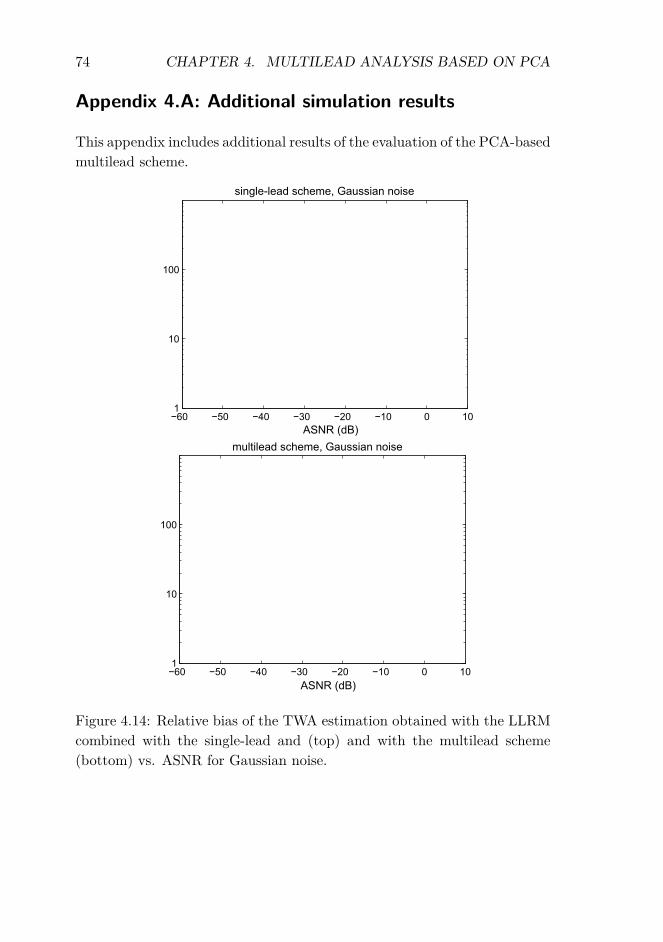
74 CHAPTER 4. MULTILEAD ANALYSIS BASED ON PCA
Appendix 4.A: Additional simulation results
This appendix includes additional results of the evaluation of the PCA-basedmultilead scheme.
Figure 4.14: Relative bias of the TWA estimation obtained with the LLRMcombined with the single-lead and (top) and with the multilead scheme(bottom) vs. ASNR for Gaussian noise.

4.6. CONCLUSIONS 75
Figure 4.15: Relative bias of the TWA estimation obtained with the LLRMcombined with the single-lead and (top) and with the multilead scheme(bottom) vs. ASNR for Laplacian noise.

76 CHAPTER 4. MULTILEAD ANALYSIS BASED ON PCA
Figure 4.16: Relative bias of the TWA estimation obtained with the LLRMcombined with the single-lead and (top) and with the multilead scheme(bottom) vs. ASNR for em noise.

4.6. CONCLUSIONS 77
Figure 4.17: Relative error of the TWA estimation obtained with the LLRMcombined with the single-lead and (top) and with the multilead scheme(bottom) vs. ASNR for Gaussian noise.

78 CHAPTER 4. MULTILEAD ANALYSIS BASED ON PCA
Figure 4.18: Relative error of the TWA estimation obtained with the LLRMcombined with the single-lead and (top) and with the multilead scheme(bottom) vs. ASNR for Laplacian noise.

4.6. CONCLUSIONS 79
Figure 4.19: Relative error of the TWA estimation obtained with the LLRMcombined with the single-lead and (top) and with the multilead scheme(bottom) vs. ASNR for em noise.

80 CHAPTER 4. MULTILEAD ANALYSIS BASED ON PCA

Chapter 5
Evaluation of the multileadscheme based on PeriodicComponent Analysis
5.1 Introduction
The evaluation study in the previous chapter demonstrated that the multi-lead scheme based on PCA improves the estimation and detection perfor-mance of SM and LLR single-lead techniques. This improvement, however,is limited by the fact that PCA uses a maximum-variance criterion to sepa-rate signal and noise into orthogonal subspaces, which may not be the bestway of differentiating between the constituent sources of an ECG signal,particularly if they are not orthogonal [Clifford et al., 2006].
In this chapter, the use of Periodic Component Analysis (πCA) for themultilead scheme is evaluated. πCA is a technique that was first proposedfor speech analysis [Saul and Allen, 2000] and then applied to the analysisof ECGs, for ECG compression and also for maternal and fetal ECG sepa-ration [Sameni et al., 2008]. With this technique, the variance criterion ofPCA is replaced by a periodical structure criterion to separate TWA fromnon-alternant components, which is a more reasonable assumption from aphysiological point of view because periodicity is the defining characteristicof TWA.
In this study, two multilead schemes, one based on πCA and one basedon PCA, are combined with the LLR method, and are compared to a con-
81

82 CHAPTER 5. MULTILEAD ANALYSIS BASED ON πCA
ventional single-lead approach, in which each ECG lead is analyzed inde-pendently. Results on simulated signals with different types of noise, realsignals with added TWA, and stress test signals, show that the πCA-basedscheme provides the best detection power and has the potential to improvethe prognostic value of TWA tests.
In addition to PCA and πCA, the use of other source separation tech-niques is explored in this chapter. In particular, the spectral ratio maximiza-tion (SRM), which is a new separation technique based on the periodicity ofthe signal, and two ICA algorithms are considered. These source separationtechniques were presented in section 3.4. In the present chapter, the detec-tion performance obtained with each technique is compared by analyzing aset of ECG signals with known TWA.
5.2 Data sets
To compare the analysis schemes in a variety of scenarios, three data setswith increasing degree of realism were analyzed. The first data set was com-posed of synthetic ECG signals with simulated TWA. In the second dataset, known TWA was added to real ECG signals. The third data set con-tained real stress test ECGs from healthy volunteers and ischemic patients.Both second and third sets were composed of the stress test ECGs from the211 patients of the non-ischemic group, the 66 asymptomatic volunteersof the volunteer group, and the 79 patients of the ischemic group in thestress test database described in section 3.5.3. Finally, the Physionet TWAdatabase (see section 3.5.4) was analyzed to facilitate future reproduction orcomparison with the methods presented here, since this dataset is publiclyavailable.
5.2.1 Synthetic signals
Synthetic 3 Frank lead ECGs were generated using an artificial multileadECG model which can exhibit realistic TWA [Clifford et al., 2010]. Thismodel generates the cardiac dipole as a sum of Gaussian kernels, and thenderives the XYZ orthogonal leads. Natural morphology changes due tointer-beat interval (RR) and respiration are incorporated from varying theGaussian amplitude and width parameters of the dipole generator. TheTWA effect is modeled as a disturbance on the T-loop of the dipole. Anexample of a synthetic ECG generated with this model is shown in figure

5.2. DATA SETS 83
5.1.
Figure 3. Example of VCG generated by model.
Figure 4. Typical alternating ‘ABAB’ TWA pattern (with23 µV amplitude) generated from our model.
other beat classes can be derived by training the HMM onreal databases.
Since our model employs a dipole representation, withan individual Dower-like transform to map the dipole ontoclinical observational axes (such as the standard 12 leadECG), correlated noise can be added in multiple dimen-sions, and hence can manifest in a realistic manner on allobservational ECG leads. Multiple noise sources can betreated as other dipole moments in the model, and the rela-tive motions of sources and sensors can be simulated usinga Givens rotation matrix to multiply the IDT [4]. Finally,clinical features of the simulated signal can be extracteddirectly from the model [11].
An open source TWA detection algorithm developed forPCinCC, which was evaluated on this model, is described
in an accompanying paper [12].
Acknowledgements
The authors were supported by the U.S. National Insti-tute of Biomedical Imaging and Bioengineering (NIBIB)and the National Institutes of Health (NIH) (grant numberR01 EB001659), the NIH Research Resource for Com-plex Physiologic Signals (grant number U01EB008577),and the Information and Communication University (ICU),Korea. The content of this article is solely the responsibil-ity of the authors and does not necessarily represent theofficial views of the NIBIB, the NIH or ICU Korea.
References
[1] McSharry PE, Clifford GD, Tarassenko L. A dynamicalmodel for generating synthetic electrocardiogram signals.IEEE Trans Biomed Eng 2003;50(3):289–294.
[2] Clifford GD, Shoeb A, McSharry PE, Janz BA. Model-based filtering, compression and classification of the ECG.Int J Bioelectromag 2005;7(1):158–161.
[3] Clifford GD. A novel framework for signal representationand source separation. Journal of Biological Systems June2006;14(2):169–183.
[4] Sameni R, Clifford GD, Shamsollahi MB, Jutten C. Multi-channel ECG and noise modeling: application to maternaland fetal ECG signals. EURASIP Journal on Advances inSignal Processing 2007;2007(43407):1–14.
[5] Moody GB. The Physionet / Computers in CardiologyChallenge 2008: T-wave alternans. Computers in Cardi-ology September 2008;35. In Press.
[6] Dower GE, Machado HB, Osborne JA. On deriving theelectrocardiogram from vectorcardiographic leads. ClinCardiol 1980;3:87.
[7] Martınez JP, Olmos S. Methodological principles of T wavealternans analysis: a unified framework. Biomedical Engi-neering IEEE Transactions on April 2005;52(4):599–613.
[8] Bousseljot R, Kreiseler D, Schnabel A. Nutzung der EKG-Signaldatenbank CARDIODAT der PTB uber das Internet.Biomedizinische Technik 1995;40(1):S317–S318.
[9] Kreiseler D, Bousseljot R. Automatisierte EKG-Auswertung mit hilfe der EKG-Signaldatenbank CARDIO-DAT der PTB. Biomedizinische Technik 1995;40(1):S319–S320.
[10] Marquardt DW. An algorithm for least-squares estimationof nonlinear parameters. SIAM Journal on Applied Mathe-matics 1963;11(2):431–441.
[11] Clifford GD, Villarroel M. Model-based determination ofQT intervals. Computers in Cardiology 2006;33:357–360.
[12] Khaustov A, Nemati S, Clifford GD. An open-source stan-dard T-wave alternans detector for benchmarking. Comput-ers in Cardiology September 2008;35. In Press.
Address for correspondence:
Gari D. Clifford, M.I.T.,77 Massachusetts Av., Cambridge, MA 02139, USA
776
Figure 5.1: Left: example of synthetic ECG generated by the multileadECG model. Right: example of TWA simulated by the multilead ECGmodel. Figures reproduced from [Clifford et al., 2008].
Five-minute signals were created with TWA amplitudes ranging from 0µV to 200 µV. For a given TWA amplitude, a total of 50 ECG records weregenerated at a sampling frequency of 500 Hz. Individual records differedin that the underlying ECGs were generated using an stochastic model ofheart rate variability (70±5 beats per minute (bpm)). Furthermore, a sumof noises was added to the signal, containing electrode motion noise (em),muscular activity noise (ma) and baseline wander (bw), all of them obtainedfrom the MIT-BIH Noise Stress Test Database (see section 3.5.5). For eachsynthetic ECG signal, two-lead segments of 5 minutes were extracted fromem, ma and bw records beginning at a random position. These records onlycontain two leads, so a third lead of spatially correlated noise was computedas the first principal component of the two available leads. Finally, the threenoise leads were scaled to obtain an SNR of 20 dB with respect to the ECG,and added to the synthetic signal.
5.2.2 Real signals with added TWA
This data set contained real 12-lead ECGs from the stress test database (seesection 3.5.3) with artificially added TWA. ECG fragments where the pres-ence of TWA was unlikely were selected from all non-ischemic and volunteerrecords. The TWA phenomenon is partially related to heart rate, and canappear in healthy subjects at fast heart rates [Cutler and Rosenbaum, 2009,Turitto et al., 2001]. Therefore, only the initial fragment in which the heart

84 CHAPTER 5. MULTILEAD ANALYSIS BASED ON πCA
rhythm was < 100 bpm was selected from each record. These fragmentswere then divided into segments of 32 consecutive beats, resulting in a totalof 1744 ECG segments.
Then, TWA was added to ECGs, with amplitudes (Valt) ranging from0 to 200 µV. To do this, the LLR method was employed to identify a real12-lead TWA waveform (twa1) in an ECG of a patient undergoing a per-cutaneous coronary intervention. The way of obtaining this waveform wasalready described in section 4.2.1. For each Valt value, the TWA waveformwas scaled and repeated with alternating sign to create a 32 beat-long TWAsignal, and then the TWA signal was added to the 1744 ECG segments. Thisprocess was repeated with two more TWA waveforms, denoted as twa2 andtwa3, which were extracted from two records of the STAFF-III databasein the same way as twa1. Figure 5.2 shows an excerpt of a real ECG of avolunteer from the stress test database, and the resulting signal after addingTWA of 200 µV to all the leads.
10 12 14 16 18 20-7
-6
-5
-4
-3
-2
-1
0
1real signal
mV
time (s)
V6
I
II
V5V4
V3
V2V1
10 12 14 16 18 20-7
-6
-5
-4
-3
-2
-1
0
1real signal with added TWA
time (s)
mV
V3
V2V1
II
I
V6
V5
V4
Figure 5.2: Left: excerpt of a real ECG from the stress test database. Right:the same ECG after adding TWA of 200 µV using waveform twa1.
5.2.3 Stress test signals
The third data set comprised all ECGs from ischemic and volunteer groupsof the stress test database. This is the same data set that was analyzed inchapter 4 (section 4.2.2).

5.3. METHODS FOR TWA ANALYSIS 85
5.2.4 Signals from the Physionet TWA database
The fourth data set of this study comprises the synthetic records of thePhysionet T-Wave alternans database (see section 3.5.4), a total of thethirty-two 12-lead ECGs containing artificial TWA in calibrated amounts,with an approximate duration of two minutes.
5.3 Methods for TWA analysis
First, three different approaches were evaluated: a multilead scheme (figure3.2) with πCA as transformation technique (we will denote this scheme asmulti-πCA), the multilead scheme with PCA (multi-PCA) already evaluatedin chapter 4, and the single-lead scheme (single). To compare the detec-tion and estimation performances of the three schemes, the first dataset—synthetic signals—was analyzed with a 16-beat analysis window (δ = 16beats), and the second dataset—real signals with added TWA—was ana-lyzed using analysis windows of K = 32, 64 or 128 beats (δ = K/2 in allcases).
Second, the simplified multilead scheme for TWA detection (figure 3.4)was combined with PCA, πCA, SRM, πCA-SRM, FastICA and JADE toevaluate the effect of each separation technique in the detection perfor-mance. In this case, the first dataset was analyzed with a 16-beat analysiswindow and δ = 16 beats with all the techniques. For the first and thesecond analyses, the initial point of ST-T complexes was set 60 ms after theQRS fiducial point.
Third, stress test records were processed with multi-πCA and singleschemes. Comparison between multi-PCA and single schemes was reportedin the previous chapter, so the multi-PCA scheme was excluded from thisstudy. From the 12-lead set, only the eight independent leads (V1 to V6, IIand II) were processed using a sliding analysis window of 128 beats and δ= 1 beat.
Fourth, the synthetic signals from the Physionet TWA database wereprocessed with multi-πCA, multi-PCA and single schemes, using an analysiswindow of 32 beats. For the third and the fourth analyses, the initial pointsof ST-T complexes were set 80 ms after the QRS fiducial point if HR ≤ 100bpm and 60 ms after the QRS fiducial point if HR > 100 bpm.

86 CHAPTER 5. MULTILEAD ANALYSIS BASED ON πCA
Input signal Transformed signal after PCA Transformed signal after πCA
mV
time (s) time (s) time (s)
a) b) c)
T7T8
T6T5
T3
T2
T1
T4
T7
T8
T6
T5
T3
T2
T1
T4
I
II
V6
V5
V3
V2
V1
V4
8 9 10 11 12 13-7
-6
-5
-4
-3
-2
-1
0
8 9 10 11 12 13
-12
-10
-8
-6
-4
-2
0
2
8 9 10 11 12 13
-20
-15
-10
-5
0
Figure 5.3: (a) The eight independent leads of a real 12-lead ECG whereTWA of 200 µV was artificially added. TWA is invisible to the naked eyedue to noise and artifacts. (b) Signal in (a) after PCA transformation.TWA is now visible in T2 through exaggerated oscillations in the amplitudeof the T wave. (c) Signal in (a) after πCA transformation. TWA is clearlyvisible in T1.
5.4 Results
5.4.1 Detection performance
As in the previous chapter, probability of false alarm (PFA) was defined asthe ratio between the number of positive TWA detections in signals withValt = 0 (false detections) and the total number of decisions made in thosesignals. Probability of detection (PD) was defined as the ratio between thenumber of positive TWA detections in signals with a given Valt and the totalnumber of decisions made in those signals. For each scheme, the detectionthreshold γ was set so that the probability of false alarm (PFA) was 0.01,and the resulting PD was compared.
Detection thresholds for multi-πCA, multi-PCA, and single schemes inthe synthetic dataset are presented in table 5.1. The resulting PD is pre-sented in figure 5.4. In the range 30 µV ≤ Valt ≤ 100 µV, the multi-πCAscheme detected alternans with amplitudes at least 15 µV lower than the

5.4. RESULTS 87
detection threshold γsingle 0.15
multi-PCA 0.19multi-πCA 0.19
SRM 0.20πca-SRM 0.20FastICA 0.18JADE 0.17
Table 5.1: Detection thresholds which are necessary to obtain a PFA = 0.01in the synthetic data set, using different schemes and a 16-beat analysiswindow (δ = 16).
K = 32 K = 64 K = 128single 0.60 0.24 0.09
multi-PCA 0.49 0.23 0.07multi-πCA 0.85 0.38 0.13
Table 5.2: Detection thresholds which are necessary to obtain a PFA = 0.01in real signals with added TWA, using different schemes and analysis windowlengths K.
single scheme for a given PD. For example, the multi-πCA scheme detectedTWA of 59 µV with a PD = 0.8, while that PD was achieved by the singlescheme only for Valt > 76 µV, which can be interpreted as a detection gainof 2.20 dB.
Real signals with added TWA were processed in the same way as syn-thetic signals. For each scheme, the detection threshold γ was set so thatPFA=0.01 (see table 5.2). Using an analysis window of 32 beats (figure5.5), TWA of 5 µV was detected with a PD = 1% by the single scheme,with a PD = 60% by the multi-PCA scheme, and with a PD = 98% by themulti-πCA scheme. Similar detection differences were found by repeatingthe analysis with the two other TWA waveforms, twa2 and twa3 (figure5.6).
To better understand the effects of PCA and πCA transformations, theevolution of the GLRT statistic (Z) in the transformed leads vs. TWAamplitude was analyzed for all signals. Figures 5.8, 5.9 and 5.10 show theevolution of Z when it is computed on an ECG without any transformation,on the same ECG after PCA transformation, and on the same ECG after

88 CHAPTER 5. MULTILEAD ANALYSIS BASED ON πCA
0 20 40 60 80 100 120 1400
0.1
0.2
0.3
0.4
0.5
0.6
0.7
0.8
0.9
1
Valt
(V)
PD
single
multi-PCA
multi-CA
Figure 5.4: PD of multi-PCA, multi-πCA and single schemes obtained in3-lead synthetic signals vs. simulated TWA amplitude. PFA = 0.01 for allschemes.
0 20 40 60 80 100 120 140 160 180 2000
0.1
0.2
0.3
0.4
0.5
0.6
0.7
0.8
0.9
1
Valt
(V)
PD
single
multi-PCA
multi-CA
Figure 5.5: PD in 12-lead real signals with added TWA with multi-PCA,multi-πCA and single schemes vs. TWA amplitude. Analysis window of 32beats and PFA = 0.01 for all schemes. TWA simulated with waveform twa1.
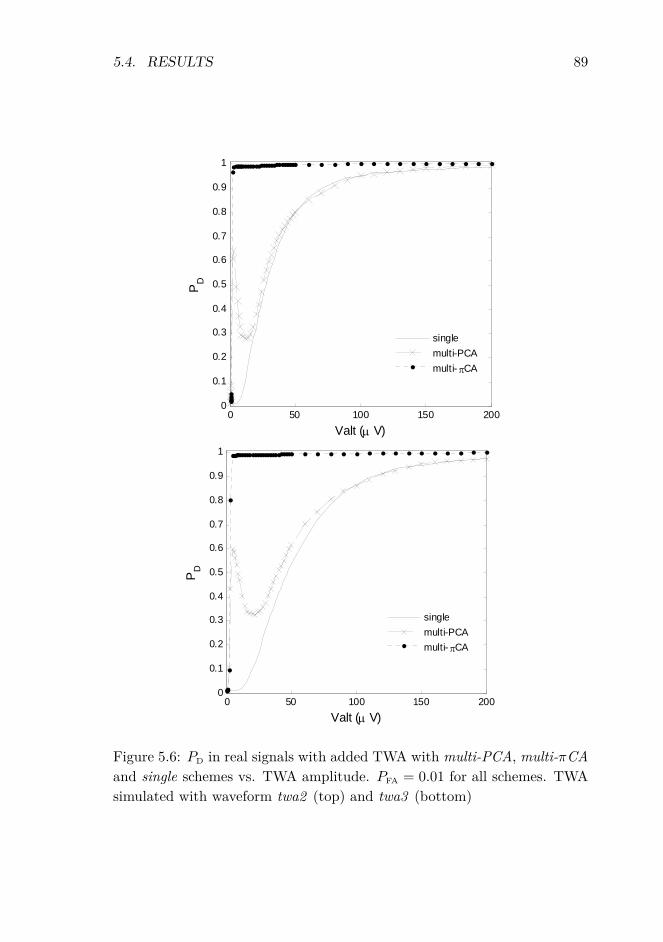
5.4. RESULTS 89
0 50 100 150 2000
0.1
0.2
0.3
0.4
0.5
0.6
0.7
0.8
0.9
1
Valt (μ V)
PD
singlemulti-PCAmulti- πCA
0 50 100 150 2000
0.1
0.2
0.3
0.4
0.5
0.6
0.7
0.8
0.9
1
Valt (μ V)
PD
singlemulti-PCAmulti- πCA
Figure 5.6: PD in real signals with added TWA with multi-PCA, multi-πCAand single schemes vs. TWA amplitude. PFA = 0.01 for all schemes. TWAsimulated with waveform twa2 (top) and twa3 (bottom)

90 CHAPTER 5. MULTILEAD ANALYSIS BASED ON πCA
0 50 100 150 2000
0.2
0.4
0.6
0.8
1
Valt (μV)
PD
singlemulti-PCAmulti-πCA
0 50 100 150 2000
0.2
0.4
0.6
0.8
1
Valt (μV)
PD
singlemulti-PCAmulti-πCA
Figure 5.7: PD in real signals with added TWA with multi-PCA, multi-πCA and single schemes vs. TWA amplitude. PFA = 0.01 for all schemes.Analysis window of 64 beats (top) and 128 (bottom). TWA simulated withwaveform twa1.

5.4. RESULTS 91
0 50 100 150 20010
-3
10-2
10-1
100
101
Valt (μV)
GLR
T st
atis
tic Z
single-lead scheme
V1V2V3V4V5V6III
0 50 100 150 20010
-3
10-2
10-1
100
101
Valt (μV)
GLR
T st
atis
tic Z
multi-PCA scheme
T1T2T3T4T5T6T7T8
0 50 100 150 20010
-3
10-2
10-1
100
101
102
Valt (μV)
GLR
T st
atis
tic Z
multi-πCA scheme
T1T2T3T4T5T6T7T8
Figure 5.8: Comparison of single (top left), multi-PCA (top right) and multi-πCA(bottom) schemes applied to the same ECG signal with different magnitudes ofTWA. The detection threshold is indicated with an horizontal straight line (PFA =0.01 for each scheme). Analysis window of 32 beats.
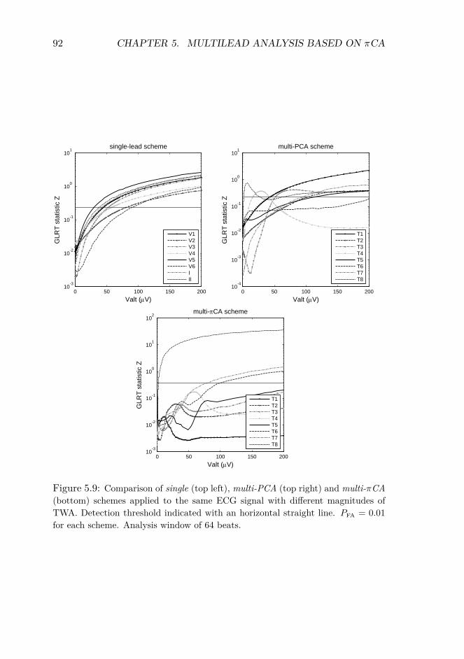
92 CHAPTER 5. MULTILEAD ANALYSIS BASED ON πCA
0 50 100 150 20010
-3
10-2
10-1
100
101
Valt (μV)
GLR
T st
atis
tic Z
single-lead scheme
V1V2V3V4V5V6III
0 50 100 150 20010
-4
10-3
10-2
10-1
100
101
Valt (μV)
GLR
T st
atis
tic Z
multi-PCA scheme
T1T2T3T4T5T6T7T8
0 50 100 150 20010
-3
10-2
10-1
100
101
102
Valt (μV)
GLR
T st
atis
tic Z
multi-πCA scheme
T1T2T3T4T5T6T7T8
Figure 5.9: Comparison of single (top left), multi-PCA (top right) and multi-πCA(bottom) schemes applied to the same ECG signal with different magnitudes ofTWA. Detection threshold indicated with an horizontal straight line. PFA = 0.01for each scheme. Analysis window of 64 beats.

5.4. RESULTS 93
0 50 100 150 20010
-3
10-2
10-1
100
101
Valt (μV)
GLR
T st
atis
tic Z
single-lead scheme
V1V2V3V4V5V6III
0 50 100 150 20010
-3
10-2
10-1
100
101
Valt (μV)
GLR
T st
atis
tic Z
multi-PCA scheme
T1T2T3T4T5T6T7T8
0 50 100 150 20010
-3
10-2
10-1
100
101
102
Valt (μV)
GLR
T st
atis
tic Z
multi-πCA scheme
T1T2T3T4T5T6T7T8
Figure 5.10: Comparison of single (top left), multi-PCA (top right) and multi-πCA (bottom) schemes applied to the same ECG signal with different magnitudesof TWA. Detection threshold indicated with an horizontal straight line. PFA = 0.01for each scheme. Analysis window of 128 beats.
94 CHAPTER 5. MULTILEAD ANALYSIS BASED ON πCA
πCA transformation, using different window lengths. In all cases, TWAis detected when Z exceeds the threshold (horizontal black line) in one ormore leads. For example, using an analysis window of K = 32 beats (figure5.8), TWA was detected by the multi-PCA scheme for Valt < 5 µV, becomeundetected for 5 < Valt < 50 µV, and then was detected again in T2 forValt = 50 µV. With πCA, TWA was detected for Valt ≥ 3.5 µV.
5.4.2 Estimation accuracy
The estimation accuracy of the schemes was also compared. For each simu-lated amplitude, the mean value and the standard deviation of the estimatedamplitude Valt was computed considering only those cases where detectionwas positive (figure 5.11). In absence of TWA, TWA was falsely detectedin 1% of the cases with a mean estimated amplitude of 142.6 µV (singlescheme) and 58.9 µV (multi-πCA scheme). For a simulated amplitude of136 µV, the bias and standard deviation of the estimation were 0.6 µV and18.2 µV respectively (single scheme), and 2.7 µV and 16.0 µV (multi-πCAscheme).
5.4.3 Comparison to other source separation techniques
The detection performance of the different transformation techniques—PCA, πCA, SRM, πCA-SRM, FastICA and JADE, presented in section3.4—was compared in the synthetic dataset, defining PD and PFA as in pre-vious sections. The best performance was obtained with schemes πCA,SRM and πCA-SRM, that presented similar PD for every Valt (figure 5.12).
The execution time (in seconds) for the analysis of the entire syntheticdataset was 64 s with PCA, 68 s with πCA, 6678 s with SRM, 5345 s withπCA-SRM, 1254 s with FastICA and 129 s with JADE.
The projection directions obtained with πCA, SRM and πCA-SRMschemes were studied. For each Valt value, the vectors w obtained witheach scheme were normalized and averaged (see sections 3.4.2 and 3.4.3).The average directions obtained with SRM and πCA-SRM schemes coin-cided in all cases. The directions of πCA and SRM schemes were similarfor low Valt (figure 5.13(a)), and the difference between them decreased asValt increased (figure 5.13(b)).

5.4. RESULTS 95
0 20 40 60 80 100 120 1400
50
100
150
200
estim
ated
Val
t (V
)
single
simulated Valt
(V)0 20 40 60 80 100 120 140
0
0.25
0.5
0.75
1
PD
0 20 40 60 80 100 120 1400
50
100
150
200
estim
ated
Val
t (V
)
multi-CA
simulated Valt
(V)0 20 40 60 80 100 120 140
0
0.25
0.5
0.75
1
PD
Figure 5.11: Estimated vs. simulated TWA amplitude in synthetic signalsusing the single-lead (top), and multi-πCA (bottom) schemes. Dots andbars represent the average and the standard deviation of the estimatedamplitude respectively, and straight line corresponds to perfect estimation(left ordinates axis). Dashed line represents the PD of each scheme forPFA = 0.01 (right ordinates axis).

96 CHAPTER 5. MULTILEAD ANALYSIS BASED ON πCA
0 50 100 150 2000
0.1
0.2
0.3
0.4
0.5
0.6
0.7
0.8
0.9
1
Valt (µV)
PD
PCAπCASRMπCA−SRMFastICAJADE
Figure 5.12: PD of the different BSS schemes vs. simulated TWA amplitude.PFA = 0.01 for all schemes.
0 0.5 10
0.5
1projection direction on the XY plane
X
Y
0 0.5 10
0.5
1projection direction on the XZ plane
X
Z
0 0.5 10
0.5
1
Y
Z
projection direction on the YZ plane
πCA
SRM
πCA-SRM
(a)
0 0.5 10
0.5
1projection direction on the XY plane
X
Y
0 0.5 10
0.5
1projection direction on the XZ plane
X
Z
0 0.5 10
0.5
1
Y
Z
projection direction on the YZ plane
πCA
SRM
πCA-SRM
(b)
Figure 5.13: Average direction of the projections obtained with the πCAscheme (squares), the SRM scheme (diamonds) and the πCA-SRM scheme(asterisks) in signals with (a) Valt=10 µV and (b) Valt=60 µV.

5.4. RESULTS 97
HRc = 100 HRc = 110single 0.09 0.10multi-πCA 0.09 0.11
Table 5.3: Detection thresholds which are necessary to obtain a PFA = 0.01in volunteer records at heart rates below a cut-off heart rate HRc, withsingle and multi-πCA schemes.
5.4.4 Application to stress test signals
Stress test signals were analyzed as reported in the previous chapter (seesection 4.3), but this time with the multi-πCA scheme. The same strategywas followed to make a fair comparison of the sensitivity of multi-πCAand single schemes: their specificity was made equal by setting the samePFA = 0.01 for both schemes. To do so, the assumption that no TWA islikely to be found in volunteer records at heart rates below a cut-off valueHRc was made. Volunteers’ signals were processed, and for each scheme thethreshold γ was calculated so that it was exceeded only by 1% of the Z valuesobtained before the heart rate reached the HRc (false detections). Then,all records from both groups were processed with the resulting thresholds,reported in table 5.3.
For each detected TWA episode, three parameters were calculated: themaximum amplitude Vmax (µV ), the duration of the episode, and the onsetheart rate HRo (bpm). Average values of amplitude, duration, and on-set heart rate were compared between volunteer and ischemic groups withthe Mann-Whitney U test, and the percentages of records with TWA ofboth groups were compared with Fisher’s exact test. A p-value < 0.05 wasconsidered significant.
First, HRc = 110 bpm was chosen in order to set γ, and all detectedTWA episodes were analyzed (table 5.4). The highest sensitivity to TWAwas obtained with the multi-πCA, since it detected TWA in more recordsthan the single scheme both in volunteer (43.9% vs. 28.7%) and in ischemicgroups (47.1% vs. 28.5%). In volunteers, TWA appeared at a lower heartrate than in ischemic patients with both schemes (126 vs. 109 bpm withthe multi-πCA scheme, 121 vs. 105 bpm with single scheme).
Then, only those TWA episodes detected before 100 bpm (first row intable 5.5) and before 110 bpm (second row in table 5.5) were analyzed. Inboth cases, the detection thresholds were computed considering cut-off heart

98 CHAPTER 5. MULTILEAD ANALYSIS BASED ON πCA
rates of HRc = 100 bpm and HRc = 110 bpm respectively for a PFA = 0.01(table 5.3). With the multi-πCA scheme, the percentage of records withTWA was significantly higher in the ischemic group in both cases, whereasthis difference was not significant with the single scheme. TWA episodesdetected by the two schemes in volunteers had lower amplitude and shorterduration than in the ischemic group, although these differences were notsignificant.
If we compare these results with those obtained in chapter 4 (table4.4), we can observe that the separation between groups is higher with themulti-πCA scheme than with the multi-PCA scheme. With the multi-πCAscheme, the percentage of records with TWA (volunteers vs. ischemics) is17% vs. 37% for HRo = 110 bpm, and 7% vs. 24% for HRo = 110 bpm,whereas with the multi-PCA these differences were lower: 9% vs. 20% forboth HRo.
5.4.5 Application to the Physionet TWA database
The Physionet T-wave alternans database (see section 3.5.4) was createdfor the Physionet challenge of 2008 [Moody, 2008]. It contains 100 records;32 of them are synthetic with known amounts of TWA, and were simulatedwith the model described in section 5.2.1, and the remaining 68 records arereal signals from different databases, 56 of which belong to patients withknown cardiac risk factors. Synthetic records have 12 leads, and real recordshave 2, 3 or 12 leads.
This database was compiled with the intention to create a reference forevaluation of new TWA algorithms. During the challenge, participants wereasked to propose a method to quantify the TWA level in the records of thedatabase, and then records were sorted according to the median TWA levelof all the entries to create a reference rank. Finally, each entry received aperformance metric computed as the Kendall’s correlation coefficient [Abdi,2007] between the method’s rank and the reference rank.
Although the reference rank was useful for scoring the challenge entries,it did not represent an increasing magnitude of TWA, and therefore it is notappropriate for benchmarking. If synthetic signals were ordered accordingto their true TWA level (correct rank), the correlation between the cor-rect rank and the reference rank derived from all entries would be 0.698,which would have been the 8th score in the competition. Furthermore, thereported method with the highest score [Bortolan and Christov, 2008] did

5.4. RESULTS 99
multi-πCA scheme single-lead schemevolunteer ischemic volunteer ischemic
% records with TWA 43.9‡ 47.1§ 28.7‡ 28.5§
TWA characteristicsVmax (µV ) 125±143 123±163 133±133 135±146
duration (s) 33±39 45±44 29±24 51±39HRo (bpm) 126±30† 109±18† 121±30† 105±20†
number of episodes 41 42 26 22
Table 5.4: Results of TWA analysis in stress test data, considering allepisodes regardless of when they are detected. PFA = 0.01 for the twoschemes. Data expressed as (mean ± one standard deviation). † indicatesa significant difference between volunteer and ischemic groups; ‡ and § in-dicate a significant difference between multilead and single-lead schemes.
multi-πCA scheme single-lead schemevolunteer ischemic volunteer ischemic
HRo < 110 bpm% records with TWA 16.6† 37.1† 9.1 17.1
Vmax (µV ) 105±107 126±169 72±55 113±55duration (s) 32±40 49±39 31±32 53±41
number of episodes 13 27 6 11
HRo < 100 bpm% records with TWA 7.5† 24.2† 7.5 14.2
Vmax (µV ) 89±87 113±143 40±20 128±130duration (s) 42±43 63±47 25±17 65±46
number of episodes 9 21 6 10
Table 5.5: Results of number of records with TWA in stress test data,calculated considering the episodes detected before heart rate reaches 110bpm (first row) and 100 bpm (second row). PFA = 0.01 for the two schemes.† indicates significant differences in the number of records with TWA involunteer and ischemic groups.

100 CHAPTER 5. MULTILEAD ANALYSIS BASED ON πCA
not quantify TWA magnitude, but only labeled records as with or withoutTWA. Besides, in the reference rank, 25 out of the 30 records with highestTWA are synthetic. This indicates that the comparison with the referencerank penalizes those methods that are able to detect TWA in real signals,and favors those methods that only measure TWA in synthetic signals witha low degree of physiological variability and with a higher number of leads.The reported method with the highest score, for instance, only detects TWAin one real signal.
These results, however, do not invalidate the use of the Physionet TWAdatabase as a reference. Comparisons can still be made with respect tothe correct rank of synthetic methods, and the fact that this dataset ispublicly available facilitates reproduction of results and comparison withother methods.
In this work, the 32 synthetic signals from this database were processedwith multi-πCA, multi-PCA and single schemes, using the detection thresh-olds computed for real signals with added TWA in section 5.4.1. ECGrecords were sorted according to the TWA amplitude estimated by eachscheme, and compared each resulting rank with the correct rank that isobtained by sorting the records according to its true TWA content. TheKendall rank correlation coefficients between the estimated rankings andthe correct ranking were 0.685 for the single scheme, 0.750 for the multi-PCA scheme, and 0.766 for the multi-πCA scheme.
5.5 Discussion
The multi-πCA scheme presents the best detection performance among thecompared schemes, both in synthetic and real signals (figures 5.4 and 5.5).This scheme exploits the fact that ECG signals do not usually contain anycomponent of cardiac origin at the frequency of 0.5 cpb other than TWA. Ifbaseline wander and other low-frequency artifacts were perfectly removed,the only component projected into the first transformed lead by the πCAtransformation would be the alternans. In practice, the signal may stillcontain residual baseline and noise after preprocessing; in that case, thetransformation does not isolate TWA in the first transformed lead, but itstill makes TWA stand out over noise, increasing the ASNR in that lead.This effect explains why TWA with an amplitude as low as 5 µV becomesdetectable in real signals (figure 5.5), and can be clearly observed in thelast panel of figure 5.8, where the detection statistic, which represents an

5.5. DISCUSSION 101
indirect measure of the ASNR, exceeds the threshold at Valt = 3.5 µV.Unlike πCA, PCA does not necessarily project the TWA component into
the first transformed lead. PCA separates signal components according totheir variance; therefore, PCA projects the component with the highestpower into the first transformed lead. That component can be the noise ifTWA power is lower than noise power.
This effect can be observed in the evolution of the GLRT statistic Zwith PCA (figure 5.8). In that example, when TWA is low (Valt = 5 µV),PCA concentrates the noise in the highest transformed leads (T1 - T3 ), re-moving it from the lowest lead (T8 ). Therefore, in T8 the ASNR rises,the statistic Z passes the detection threshold, and TWA is detected. AsValt increases, TWA and noise power become similar, and PCA cannot sep-arate them, so the ASNR in the transformed leads does not increase andTWA is not detected. Then, when Valt is high enough, TWA power startsto be higher than noise power, and PCA progressively projects TWA intohigher leads, making them detectable first in T2 and finally in T1. This“positive-negative-positive” detection pattern was consistently found in realsignals with added TWA, and is the cause of the “valley” in the PD curve ofthe multi-PCA scheme (figure 5.5). This pattern was not found in the syn-thetic signals of the first dataset, where three leads are not rich enough ininformation for PCA to produce such a clear separation of TWA and noise.The value of the detection threshold for a fixed PFA decreases when a longeranalysis window is used, but longer windows have little effect on the spatialredistribution of TWA and noise in the transformed signal. Therefore, the“valley” in the PD curve tends to disappear for longer analysis windows (seefigure 5.7).
When we compare the detection gains of multilead schemes over a single-lead scheme in the different evaluation datasets, both in this chapter and inchapter 4 (figures 4.5, 5.4 and 5.5), we can observe that the detection gainis higher for 12-lead ECGs than for 3-lead ECGs, and also that the highestdifference between single and multilead schemes is obtained with syntheticsignals without any physiological variability (the signals generated in section4.2.1). A lower number of leads and a more realistic noise and variability inthe ECG decrement the detection gain that can be obtained with a multileadscheme.
The ICA algorithms, FastICA and JADE, present the worst detectionperformance among the compared schemes (figure 5.12). ICA has been suc-cessfully applied to other ECG problems in the past [Castells et al., 2007],

102 CHAPTER 5. MULTILEAD ANALYSIS BASED ON πCA
but, according to the results of the present study, it is not the best ap-proach for TWA analysis. FastICA and JADE algorithms are based on theclassic ICA model, which assumes that the input signal is an instantaneousstationary linear mixture of independent sources, whose number equals thenumber of signal channels. This is not a very realistic assumption for TWAanalysis in 3-lead ECGs, in which the signal after the preprocessing stages,besides the TWA component, may still contain different types of residualnoise (electrode movement, baseline wander, motion artifacts) and residualactivity of the ventricles due to a non-perfect detrending filter. In this case,assuming only three sources could be unrealistic, and independence betweensources is not assured either. ICA algorithms could yield better results with12-lead ECGs, such as those obtained in TWA clinical stress tests, but theirutility with ambulatory 2 or 3-lead ECGs seems limited.
The best detection performance is obtained with the periodicity-basedschemes. Both πCA and SRM search for the direction from which theperiodicity of the transformed signal is maximum, following a temporal anda spectral criterion respectively. These criteria offer equivalent detectionresults; the directions obtained by the two schemes tend to converge as TWAincreases, and for low Valt values, πCA and SRM directions are close enoughto produce the same PD. The projections obtained with SRM and πCA-SRMschemes coincide in all cases. Initializing the optimization algorithm withπCA —a closer point to the solution— reduces convergence time, but evenin that case the computational cost is more than 70 times higher than thecost of the πCA scheme.
The main benefits of the multi-πCA scheme can also be expected whenit is combined with single-lead techniques other than the LLR method. Theimprovement in the detection power is due to the signal transformationstage, and does not depend on the actual detection technique, so similardetection gains are obtained when the multilead scheme is combined withLLR and SM techniques, as it was demonstrated in the previous chapter.Furthermore, the multi-πCA scheme can also simplify the detection rules ofexisting methods such as SM, which require a complex set of lead-specificconditions to determine the presence of TWA in an ECG [Bloomfield et al.,2002]. The fact that πCA always projects TWA into the first transformedlead (T1 ) means that the detection rule needs to be applied only to thatlead, making a simpler and more powerful detection scheme.
In addition to a high sensitivity to TWA, an accurate estimation of theTWA amplitude is also an important requisite of the analysis methods, since

5.5. DISCUSSION 103
quantitative evaluation of TWA has been shown to improve risk assessment[de Vilhena Garcia et al., 2009, Minkkinen et al., 2008, Klingenheben et al.,2005]. Results in section 5.4.1 indicate that the multi-πCA scheme improvesthe accuracy of the amplitude estimation (figure 5.11). For high Valt levels,the bias of the multi-πCA estimation is slightly higher than the bias of thesingle-lead estimation due to the truncation carried out in the reconstructionstage —as only a subset of transformed leads is used to reconstruct thesignal, the reconstructed TWA lacks the content of the truncated leads,which may still contain a small alternant component. However, the varianceof the multi-πCA estimation is lower than the variance of the single-leadestimation, especially at low amplitudes, so the total mean square error isalways lower than with the single scheme. This effect is also observed in thePhysioNet TWA database, where the use of the multi-πCA scheme providesthe highest correlation with the correct rank of records.
Results on stress test signals confirm that the higher sensitivity to TWAof the multi-πCA scheme can also be expected in a real clinical dataset.Furthermore, this scheme improves the differentiation of volunteers and is-chemic patients according to TWA episodes over the multi-PCA and thesingle schemes, which indicates the potential clinical utility of the proposedmethod. According to current guidelines of TWA analysis in stress test,TWA episodes are considered to indicate arrhythmic risk only if they satisfyseveral requirements, one of them being longer than 60 seconds [Bloomfieldet al., 2002]. These guidelines have been derived after extensive applicationof the spectral method in clinical studies, and their application to othertechniques is not straightforward, but needs to be clinically validated be-fore extracting conclusions about the prognostic value of any new method.In our study, results indicate that TWA appears at higher heart rates involunteers than in ischemic patients, and that under heart rates of 100 and110 bpm, TWA episodes are less frequent and have lower amplitude andshorter duration (around 30 seconds) than in the ischemic group. Thesefindings agree with existing clinical evidence [Nearing and Verrier, 2002,Rosenbaum et al., 1994], but it would be premature to extract conclusionsabout arrhythmic risk at this stage.
In this study, cut-off values of heart rate, amplitude or duration of TWAto predict cardiovascular events could not be determined in the study pop-ulation because the follow-up information in terms of arrhythmic events orall-cause mortality was not available.

104 CHAPTER 5. MULTILEAD ANALYSIS BASED ON πCA
5.6 Conclusions
The multilead analysis scheme based on πCA is the most robust and sensi-tive tool for TWA analysis among the compared alternatives. Comparisonin different scenarios—from synthetic signals to clinical records—shows thatit provides a better detection power than the previously proposed multileadscheme based on PCA, and than the conventional single-lead approach. Fur-thermore, the proposed scheme improves the differentiation between healthyvolunteers and patients with ischemic disease according to TWA detections.
Chapter 6
Analysis of TWA in ambulatoryrecords
6.1 Introduction
The utility of TWA testing during ambulatory monitoring has been subjectto intense investigation in recent years [Verrier et al., 2005b, Nieminen andVerrier, 2010]. In ambulatory records, the maximum amplitude of TWAhas been semi-automatically quantified using the Modified Moving AverageMethod MMAM [Verrier et al., 2005b], and then compared to a cut pointto decide if such TWA level should be considered normal or abnormal. Thisbinary TWA index has been found to be a strong predictor of arrhythmicevents and cardiac mortality in different populations [Nieminen and Ver-rier, 2010]. In the last years, quantitative analysis of TWA amplitude as acontinuous variable has also been shown to indicate an increasing cardiacrisk [Klingenheben et al., 2005, Slawnych et al., 2009].
The MMAM measures the local TWA activity at each analysis pointusing the powerful noise-rejection principle of recursive averaging [Verrieret al., 2005b]. However, as only one TWA measurement is usually chosento characterize an ambulatory record, it is essential that this measurementcorresponds to real TWA and that it is not caused by artifacts in the signal.Therefore, the visual verification of TWA measurements after MMAM pro-cessing becomes indispensable [Nieminen and Verrier, 2010]. Furthermore,basing the risk assessment on a single TWA measurement may reduce thereproducibility of the index, as it is very dependent on the specific activitythat the patient is performing at a particular time.
105

106 CHAPTER 6. ANALYSIS OF TWA IN AMBULATORY RECORDS
One way to circumvent these limitations could be to extend the averag-ing approach to longer periods. It has been shown that long-term averagingof ECG measurements allows the quantification of subtle phenomena suchas heart rate turbulence [Martínez et al., 2010], deceleration capacity [Baueret al., 2006] or baroreflex sensitivity [Rienzo et al., 2001]. The hypothesisof the study in this chapter is that the application of extensive, long-termaveraging to TWA quantification will produce reliable measurements of theaverage TWA activity over long periods, and that these measurements, be-ing less sensitive to noise, will make it possible to perform TWA analysisfor risk assessment in a fully-automated way.
This study presents a fully-automated method to analyze TWA in am-bulatory records, based on the πCA multilead scheme, which was chosenas the best option among the alternatives compared in chapter 5. Resultsdemonstrate that the average TWA activity in a 24-hour period is an in-dependent predictor of CD and SCD in patients with chronic heart failure(CHF). Following the approaches of existing studies [Klingenheben et al.,2005, Slawnych et al., 2009, Minkkinen et al., 2009], two risk indices areproposed: a binary index that defines a positive/negative TWA test, and aquantitative continuous index that reflects an increasing degree of cardiacrisk.
6.2 Study population
A total of 992 patients with symptomatic CHF corresponding to NYHAclasses II to III were enrolled in the MUSIC (MUerte Súbita en InsuficienciaCardiaca) study, a prospective, multicenter study designed to assess riskpredictors for cardiovascular mortality in ambulatory patients with CHF[Vázquez et al., 2009]. The study protocol was approved by institutionalinvestigation committees and all patients signed informed consent. Thecollection of clinical data for this population was reported in previous studies[Vázquez et al., 2009, Cygankiewicz et al., 2009]. No medications werewithdrawn during Holter monitoring.
Twenty-four-hour ambulatory ECG recordings (XYZ orthogonal leads,200 Hz sampling rate) were performed using SpiderView recorders (ELAMedical, Sorin Group, Paris, France). From the overall population, the650 available records from patients with sinus rhythm were included in thepresent study. The clinical characteristics of studied patients as well asmedication are listed in the first column of table 6.1.

6.3. METHODS 107
6.2.1 Follow-up and end-points
Patients were followed up every 6 months for a median of 48 months, withtotal mortality as a primary end point, and cardiac death (CD) and sud-den cardiac death (SCD) as secondary end points. Information about endpoints was obtained from medical records, patients’ physicians, and familymembers.
Cardiac death was defined as death from cardiac causes, but exclud-ing such vascular causes as pulmonary embolism, aortic aneurysm dissec-tion/aneurysm, or stroke. Sudden cardiac death was defined as: a) a wit-nessed death occurring within 60 minutes from the onset of new symptomsunless a cause other than cardiac was obvious, b) an unwitnessed death(< 24 hours) in the absence of preexisting progressive circulatory failure orother causes of death, or c) death during attempted resuscitation.
End points were reviewed and classified by the MUSIC Study EndpointCommittee. Table 6.2 summarizes the number of deaths in the study pop-ulation during the median 48-month period.
6.3 Methods
6.3.1 Measurement of TWA
The analysis scheme chosen for this study is the multilead scheme basedon πCA. Instead of using the general multilead scheme (figure 3.2), themodified scheme depicted in figure 3.5 is used, because in this case thedetection threshold cannot be realistically determined. In previous studies,a threshold for the detection stage was set by analyzing signals withoutTWA (in data sets with artificially added TWA), or ECG segments fromhealthy subjects where the absence of TWA could be reasonably assumed(in stress test data). In the present study, the absence of TWA could notbe assumed at any point because the population did not include a controlgroup of healthy subjects. Choosing a threshold from previous studies wasnot realistic either, because thresholds depend on factors such as the numberof leads to analyze, the conditions of ECG recording (rest vs. stress test, forexample), and the length of the analysis window, among others. Therefore,the modified scheme in which detection is omitted was selected.
Heart beats were detected and labeled as normal or abnormal with theAristotle ECG analysis software [Moody and Mark, 1982]. Baseline wan-

108 CHAPTER 6. ANALYSIS OF TWA IN AMBULATORY RECORDS
der was canceled using a cubic-splines technique [Meyer and Keiser, 1977].Automatic TWA analysis was then performed on every ECG recording inthree steps: 1) selection of signal segments which were suitable for auto-matic analysis, 2) estimation of the amplitude of TWA in those segments,and 3) computation of indices that reflect the general alternans activitythrough the record. These steps are summarized below.
Selection of segments
ECGs were analyzed in segments of 128 beats with a 50% overlap betweenadjacent segments (δ = 64). Each segment was included in automatic TWAanalysis if 1) the difference between the maximum and the minimum in-stantaneous heart rate (HR) during the segment was ≤ 20 beats per minute(bpm), and 2) at least 80% of the beats in the segment fulfilled all of thefollowing conditions:
1. it was labeled as normal by the Aristotle software,
2. the difference between the RR interval of that beat and the previousRR interval was ≤ 150 ms,
3. the difference between the baseline voltage measured at the PQ seg-ment in that beat and the one measured in the preceding beat was ≤300 µV.
Estimation of TWA amplitude
If an ECG segment (denoted as the kth segment) was suitable for analysis,a measurement of the TWA amplitude in that segment (denoted as Vk) wascomputed by using a multilead scheme that combined πCA with the LLRM.
First, the ECG segment was low-pass filtered at 15 Hz to eliminate partof the noise that could affect the estimation of TWA amplitudes. Figure 6.1shows an example of an ECG signal with TWA after baseline cancellationand low-pass filtering.
Then, the three orthogonal leads of the ECG segment were linearlycombined to obtain a new lead in which the visibility of TWA over noisewas maximized. This combination of leads was not predetermined, butwas specifically computed for each segment with the πCA technique, anddepended on how the 2-beat periodic components of the signal were dis-tributed among the ECG leads. In this study, only the first transformed

6.3. METHODS 109
-4
linear combination
with πCA
89 90 91 92 93
0
0.5
1
mV
time (s)
combined
lead. . .
mV
time (s)
X
Y
Z
. . .
. . .
. . .
kth segment (128 beats)
estimation of
TWA waveform
0 100 200 3000
20
40
60
80
ST-T complex (ms)
estim
ated
TW
A (µ
V)
Vk
89 90 91 92 93
-3
-2
-1
0
1
TWA amplitude
for kth segment
c)
a)
b)
Figure 6.1: Example of TWA amplitude estimation. (a) ECG segmentselected for automatic analysis after low-pass filtering and baseline cancel-lation. (b) New combined lead, computed with πCA. (c) Median TWAwaveform in the segment, estimated with the Laplacian likelihood ratiomethod, and absolute TWA amplitude in the segment Vk = 18.5 µV.

110 CHAPTER 6. ANALYSIS OF TWA IN AMBULATORY RECORDS
obtained with πCA was analyzed, since it is the lead where TWA is pro-jected, as demonstrated in chapter 5. Figure 6.1(b) shows the combinedlead obtained with πCA for the example ECG segment.
Finally, TWA amplitude was measured in the new combined lead (not ina reconstructed signal, this is the main difference with the general multileadscheme). In each beat, an interval of 350 ms after the end of the QRS wasselected (ST-T complex, marked with dashed lines in figure 6.1(b)). Themedian difference between the ST-T complexes of even and odd beats wascomputed by using the LLRM. In this way, an estimation of the medianTWA waveform in the ECG segment was obtained (figure 6.1(c)). Theamplitude of TWA in the segment, denoted as Vk, was finally measuredas the absolute value of the mean of the estimated TWA waveform (figure6.1(c)).
Computation of TWA indices
Two sets of indices were computed after measuring the amplitude of TWA inall the segments of an ECG record. The first set reflected the average activ-ity of TWA within the segments under study, and the second set quantifiedthe maximum TWA amplitude in the segments under study.
The first set consisted of the Average Alternans Index (AAI) and theheart-rate-restricted Average Alternans Indices (AAIx). AAI was computedas the average of all Vk values in the ECG signal, and reflected the averageTWA activity during the 24-hour period. Note that, for instance, a 24-hourECG that presented TWA only during 5% of the time with an amplitudeof 60 µV would have an AAI = 3 µV, which means that the AAI cannotbe interpreted as a direct measurement of the amplitude of TWA at anysingle point. Restricted Average Alternans Indices (AAIx) were computedas the average of only those Vk values measured in segments with averageHR ranging from X -10 bpm to X bpm, with X= {70, 80, 90, 100, 110}. Forinstance, AAI90 would reflect the average TWA activity at HR between 80and 90 bpm in the 24-hour period.
The second set consisted of the Maximum Alternans Index (MAI) andthe restricted Maximum Alternans Indices (MAIx). MAI was computedas the maximum of all Vk values in the ECG signal. Restricted MaximumAlternans Indices (MAIx) were computed as the maximum of the Vk valuesmeasured in segments with average HR ranging from X -10 bpm to X bpm,with X= {70, 80, 90, 100, 110}. For instance, MAI90 would represent the
6.4. RESULTS 111
maximum TWA amplitude at HR between 80 and 90 bpm in the 24-hourperiod. This set of indices quantifying maximum TWA amplitudes wasincluded for comparison to the usual approach in ambulatory TWA testing.
6.3.2 Statistical analysis
Data are presented as mean ± standard deviation for continuous variables,and number and percentage for categorical variables. Two-tailed Mann-Whitney and Fisher’s exact tests were used for univariate comparison ofquantitative and categorical data respectively. Survival probability was es-timated using Kaplan-Meier methods with comparison of cumulative eventsusing log-rank tests. Univariate and multivariate Cox proportional hazardsanalyses were performed to determine the prognostic value of TWA indicesin predicting the end points. Cox regression models were built considering asignificance ≤ 0.05 as the criterion for entry into a model. Linear relationsbetween quantitative TWA indices and HR were evaluated with Spearman’scorrelation coefficient. A p-value < 0.05 was considered statistically signif-icant. Data were analyzed using SPSS software (version 15.0; SPSS Inc.Chicago, IL).
6.4 Results
The mean value of AAI in the study population was 3.3 ± 2.1 µV, and the25th, 50th and 75th percentiles were 2.4, 2.9 and 3.7 µV respectively (figure6.2). A weak negative correlation was found between AAI and mean HR inthe Holter recording (ρ = -0.083, p-value = 0.035).
Patients were divided into TWA positive (TWA+) and TWA negative(TWA-) groups by setting a cut point for AAI of 3.7 µV, corresponding tothe 75th percentile of the distribution of AAI in the population. Of the 650studied patients, 493 (75.8%) were included in the TWA- group (AAI ≤ 3.7µV) and 157 (24.2%) in the TWA+ group (AAI > 3.7 µV). No significantdifferences were found upon comparison of clinical variables in TWA+ andTWA- groups (table 6.1). Survival rate was significantly higher in groupTWA- for primary and secondary end points (table 6.2). Figure 6.3 showsthe distribution of AAI in survivors, CD and SCD groups.
Univariate Cox analysis revealed that a TWA+ outcome was associatedto all-cause mortality, to CD, and to SCD (table 6.3). No association wasfound between a TWA+ outcome and non-cardiac mortality. Multivari-

112 CHAPTER 6. ANALYSIS OF TWA IN AMBULATORY RECORDS
0
5
10
15
µV
AAI AAI70
AAI80
AAI90
AAI100
AAI110
650 (100) 532 (82) 591 (91) 563 (87) 460 (74) 343 (53)
**
**
**
*
mean 70 80 90 100 110
0
10
20
30
40
50
60
70
µV
MAI MAI70
MAI80
MAI90
MAI100
MAI110
650 (100) 643 (99) 591 (91) 563 (87) 460 (74) 343 (53)
**
Figure 6.2: Top: boxplot of the average alternans indices computed in the24-h period (AAI), and in intervals with HR in the range of X -10 to X bpm(AAIx). Bottom: boxplot of the maximum alternans indices computed inthe 24-h period (MAI), and in intervals with HR in the range of X -10 toX bpm (MAIx). The number (and percentage) of records in which indicescould be computed is indicated above the boxes. Significant differencesbetween the medians of adjacent boxes are indicated by *(p < 0.05) and**(p < 0.001).

6.4. RESULTS 113
survivors CD SCD0
1
2
3
4
5
6
7
8
µV
AAI
Figure 6.3: Boxplot of the average alternans index computed in the 24-hperiod (AAI) in survivors, CD and SCD groups. The horizontal dashed lineindicates the cut point of 3.7 µV, corresponding to the 75th percentile ofthe distribution of AAI in the overall population.
ate Cox proportional hazards models were constructed by adjusting for (1)age, gender, NYHA class, LVEF < 35%, and diabetes, and (2) use of beta-blockers, amiodarone and ACE or ARB inhibitors in addition to covariablesin model (1). For multivariate model (1), a TWA+ outcome was the vari-able most significantly associated to SCD risk, with a hazard ratio of 2.38,similar to LVEF < 35% (hazard ratio 2.55, 95% CI: 1.35 – 4.80, p = 0.004).For multivariate model (2), a TWA+ outcome was the covariable with thesecond highest hazard ratio (2.29) after LVEF < 35% (hazard ratio 2.65,95% CI: 1.39 – 5.03, p = 0.003). The event-free curves for CD and SCD areshown in figure 6.4.
The mean values of AAIx were AAI70 = 2.8 ± 1.9 µV, AAI80 = 3.3± 2.3 µV, AAI90 = 3.9 ± 2.4 µV, AAI100 = 5.0 ± 3.1 µV and AAI110= 6.1 ± 5.5 µV. Not all ECGs presented a HR spanning from 60 to 110bpm; also, all segments within a certain HR range were discarded for TWAanalysis in some recordings (according to the inclusion rules described in theMethods section). Therefore, not every AAIx could be computed for everypatient. The percentages of indeterminate values for the entire populationwere 18.1% for AAI70, 9.1% for AAI80, 13.4% for AAI90, 26.1% for AAI100,

114 CHAPTER 6. ANALYSIS OF TWA IN AMBULATORY RECORDS
TotalPopulation TWA− TWA+(n = 650) (n = 493) (n = 157) p
Age (years) 63 ± 12 63 ± 11 64 ± 13 0.091Gender (men) 462 (71.1%) 350 (71.0%) 112 (71.3%) 0.999
NYHA class III 117 (18.0%) 87 (17.6%) 30 (19.1%) 0.721LVEF < 35% 356 (54.8%) 262 (53.1%) 94 (59.9 %) 0.142
Diabetes 245 (37.7%) 190 (38.5%) 55 (35.0%) 0.451Beta-blockers 454 (69.8%) 350 (71.0%) 104 (66.2%) 0.273Amiodarone 59 (9.1%) 43 (8.7%) 16 (10.2%) 0.632
ARB or ACE inhibitors 573 (88.2%) 441 (89.4%) 132 (84.1%) 0.088Average HR (bpm) 75 ± 12 76 ± 12 75 ± 12 0.581
Maximum HR (bpm) 122 ± 26 123 ± 27 119 ± 25 0.100
NYHA = New York Heart AssociationLVEF = Left ventricular ejection fractionARB = Angiotensin receptor blockerACE = Angiotensin-converting enzyme
Table 6.1: Characteristics of patients. Data are presented as absolute fre-quencies and percentages, or as mean ± standard deviation.
Total Population TWA− TWA+(n = 650) (n = 493) (n = 157) p
Total mortality 146 (22.5%) 99 (20.1%) 47 (30.0%) 0.012CD 119 (18.3%) 81 (16.4%) 38 (24.2%) 0.033
SCD 52 (8.0%) 30 (6.1%) 22 (14.0%) 0.003
Table 6.2: Events during follow-up. Data expressed as absolute frequenciesand percentages.

6.4. RESULTS 115
AAI > 3.7 µV AAI90Total mortality Hazard ratio p Hazard ratio p
Univariate 1.62 (1.15 − 2.29) 0.006 1.04 (0.99 − 1.10) 0.150Multivariate(1) 1.54 (1.09 − 2.19) 0.015 1.05 (0.98 − 1.11) 0.144Multivariate(2) 1.48 (1.04 − 2.10) 0.030 1.04 (0.98 − 1.11) 0.184
AAI > 3.7 µV AAI90CD Hazard ratio p Hazard ratio p
Univariate 1.60 (1.09 − 2.35) 0.017 1.05 (1.00 − 1.11) 0.051Multivariate(1) 1.54 (1.04 − 2.26) 0.030 1.06 (1.00 − 1.13) 0.038Multivariate(2) 1.44 (0.97 − 2.13) 0.068 1.06 (1.00 − 1.13) 0.051
AAI > 3.7 µV AAI90SCD Hazard ratio p Hazard ratio p
Univariate 2.48 (1.43 − 4.30) 0.001 1.07 (1.01 − 1.15) 0.041Multivariate(1) 2.38 (1.37 − 4.14) 0.002 1.07 (1.00 − 1.15) 0.039Multivariate(2) 2.29 (1.31 − 4.00) 0.004 1.07 (1.00 − 1.15) 0.046
Table 6.3: Association of TWA indices with mortality. 95% confidence inter-vals for hazard ratios are reported in brackets. Adjusted multivariate model(1) includes age, gender, NYHA class, LVEF < 35%, and diabetes. Adjustedmultivariate model (2) includes covariables in (1) plus use of betablockers,amiodarone, and ARB or ACE inhibitors.

116 CHAPTER 6. ANALYSIS OF TWA IN AMBULATORY RECORDS
19
Time (days)
1400120010008006004002000
Cum
ulat
ive
surv
ival
1,0
0,9
0,8
0,7
0,6
TWA +
TWA -
Time (days)
1400120010008006004002000
Cum
ulat
ive
surv
ival
1,0
0,9
0,8
0,7
0,6
TWA +
TWA -
p = 0.001
p = 0.016
Sudden Cardiac Death
Cardiac Death
Figure 6.4: Event-free curves for CD (top) and SCD (bottom).

6.5. DISCUSSION 117
and 47.2% for AAI110. Figure 6.2 shows the distributions of AAIx.The mean values of AAIx increased with HR, and there were signifi-
cant differences between indices from all adjacent HR intervals (figure 6.2).Univariate Cox analysis was performed for all AAIx, and only AAI90 wasfound to be associated with SCD. Multivariate Cox analysis confirmed thisassociation (table 6.3). AAI90 was not associated to all-cause mortality ornon-cardiac mortality.
The mean value of MAI in the study population was 31.4 ± 25.3 µV, andthe 25th, 50th and 75th percentiles were 17.9, 24.7 and 38.0 µV respectively(figure 6.2). No association to CD or SCD risk was found for MAI as acontinuous variable or as a categorical variable after dichotomization withthe 75th percentile. The mean values of MAIx were MAI70 = 16.1 ± 13.1µV, MAI80 = 17.2 ± 10.6 µV, MAI90 = 17.5 ± 12.1 µV, MAI100 = 19.7± 12.1 µV and MAI110 = 20.6 ± 22.6 µV. MAIx were not significantlyassociated to CD or SCD risk according to Cox univariate and multivariateanalyses.
6.5 Discussion
This study demonstrates that the quantification of the average TWA activ-ity over long periods is a strong, independent predictor of SCD in patientswith CHF. Two indices quantifying the TWA activity in a 24-hour period,AAI and AAI90, were found to independently predict CD and SCD, but didnot predict non-cardiac mortality, a finding that supports the hypothesisthat elevated TWA activity reflects abnormal cardiac function predisposingto cardiac death.
The average TWA activity in a 24-h period, quantified by the AAI, wasthe covariable most strongly associated to the risk of SCD. In our popu-lation, only a weak correlation was found between AAI and the patient’sHR, which indicates that AAI is not merely a surrogate measure of thepatient’s HR, but also reflects the influence of HR-independent factors inTWA. Therefore, AAI may provide a measure of the extent of cardiac vul-nerability, because a higher influence of HR-independent factors in TWAamplitude reflects a higher degree of cardiac electrical instability [Verrieret al., 2009].
The prognostic value of quantitative TWA measurements is increasinglybeing studied [Klingenheben et al., 2005, Slawnych et al., 2009, Minkkinen

118 CHAPTER 6. ANALYSIS OF TWA IN AMBULATORY RECORDS
et al., 2009]. In this study, an index of quantitative TWA (AAI90) inde-pendently predicted SCD. When measured at moderate heart rates, highermagnitudes of TWA are known to predict a greater risk of serious outcomes[Cutler and Rosenbaum, 2009]. For TWA to predict cardiovascular events,maximum HR limits ranging from 100 to 125 bpm are usually considered[Verrier et al., 2009]. In this study, we found that the average TWA activitywas associated to SCD when measured at lower rates, between 80 and 90bpm (AAI90). A possible explanation for this difference is that heart failurelowers the HR threshold to elicit TWA [Wilson et al., 2009].
Unsupervised maximum TWA amplitudes, measured by MAI and MAIx,did not predict cardiac risk. Although the values obtained for MAI werecomparable to maximum TWA amplitudes reported in the literature (be-tween 30 and 60 µV), no significant association was found between MAI andrisk of SCD or CD. This was not unexpected, since it is known that mea-suring TWA amplitudes without testing for its significance, either visuallyor automatically, can lead to inaccurate results due to noise and artifacts[Nemati et al., 2010]. In recent studies with ambulatory ECGs, the maxi-mum TWA amplitude in a record is measured with the MMAM, either inthe whole record [Maeda et al., 2009] or in segments below a maximum HR[Sakaki et al., 2009], and then needs to be visually verified to ensure thatthey correspond to real TWA.
In the present study, we found that quantifying the average TWA ac-tivity (AAI) instead of the maximum amplitude (MAI) eliminates the ne-cessity of visually discarding erroneous measurements, and allows the pre-diction of CD and SCD in the study population. To our best knowledge,the method presented in this work is the first one that allows a multilead,fully-automated computation of TWA markers of cardiac risk in ambula-tory ECGs. However, although this study indicates that the average TWAactivity over a 24-hour period provides important prognostic information inpatients with CHF, it would be premature to extend these observations toother groups. The use of a 75th percentile cut point for TWA measures isa common starting point when a technique is first tested on a population[Verrier and Nearing, 2003, Nieminen et al., 2007], but additional prospec-tive evaluation is still required, particularly on the applicability of the cutpoint derived in this study.

6.6. CONCLUSIONS 119
6.6 Conclusions
This study demonstrates that the improvements in TWA detection andestimation obtained with the πCA multilead scheme, together with the pro-posed strategy for computing global TWA indices, make it possible to strat-ify cardiac risk in Holter recordings without the need for visual validation.Results show that the average TWA activity over a 24-hour period providesimportant prognostic information in patients with CHF. Two novel indices,AAI and AAI90, have been proposed to quantify the average TWA activity,and have been found to independently predict the risk of CD and SCD.

120 CHAPTER 6. ANALYSIS OF TWA IN AMBULATORY RECORDS

Chapter 7
Conclusions
This chapter summarizes the original contributions and main conclusions ofthe thesis, and proposes possible extensions of the work.
7.1 Summary and conclusions
As stated in chapter 1, the objective of this thesis was to develop a multileadscheme for TWA analysis that improved the detection and quantification ofTWA in the ECG, and that increased the clinical value of TWA as a riskindex. The work carried out to achieve this goal can be divided in threeparts: design of novel multilead schemes for TWA analysis, methodologicalevaluation of the proposed techniques, and clinical validation of the selectedmultilead scheme. The original contributions and conclusions of each partare summarized next.
Design of novel multilead schemes for TWA analysis
Chapter 3 introduced a general scheme for multilead analysis of TWA. Theproposed scheme is an extended version of a usual single-lead scheme, wheretwo additional stages, transformation and reconstruction, increase the de-tectability of TWA, and also improve the estimation of TWA amplitude andwaveform. Various techniques are proposed for the transformation stage(PCA, πCA, ICA and SRM). While πCA and ICA techniques are not new,they have been applied to TWA analysis for the first time in this work. SRMis a new technique proposed in this work which exploits the periodicity ofTWA to increase its detectability in the transformed signal.
121

122 CHAPTER 7. CONCLUSIONS
The general multilead scheme is not tied to a specific TWA analysismethod, but can be combined with any single-lead method which detectsand estimates TWA in separate stages. Along the thesis, it has been com-bined with the LLRM, and also with the SM for comparison. Besides,several modifications are proposed to adapt the general scheme to differentclinical settings.
Methodological validation
Chapters 4 and 5 presented the methodological evaluation of the multileadscheme based on PCA (multi-PCA scheme) and based on πCA (multi-πCAscheme). Multi-PCA, multi-πCA and single-lead schemes were comparedin various simulation studies, in which synthetic, semi-synthetic and realsignals with known TWA were analyzed. Differences between schemes werequantified using two common performance metrics, probability of detectionand probability of false alarm, and also using new global measures of thebias and variance of the TWA estimation. Differences in the detection powerobtained with πCA and with other BSS techniques were also studied.
Simulation results in chapter 4 showed that the multi-PCA scheme de-tects TWA with a SNR 30 dB lower, and estimates TWA with a SNR 25dB lower than the single-lead scheme for a given false alarm rate. It wasalso shown that a similar detection gain can be obtained by applying themulti-PCA scheme to the SM.
According to results in chapter 5, the multi-πCA is the one which pro-vides the best detection power among the compared alternatives. In realstress-test signals with added TWA, and for a 1% false alarm rate, themulti-πCA scheme detects TWA of 5 µV with a probability of 98%, whilethe probabilities for multi-PCA and single schemes are 60% and 1% respec-tively.
When comparing BSS techniques, results in chapter 5 showed that theperiodicity-based schemes (πCA and SRM) yield the best detection power.The maximum detection performance is obtained either using a temporalcriterion (πCA) or a spectral criterion (SRM) to maximize the periodicity ofthe transformed signal. Therefore, using periodicity to separate TWA fromnoise is the best multilead strategy among the compared options. BetweenπCA and SRM, πCA is a better option because its computational cost ismuch lower.
Multi-PCA, multi-πCA and single-lead schemes were used to analyze

7.2. FUTURE WORK 123
a stress test database. Results in chapter 4 showed that it is possible todistinguish between CAD patients and healthy volunteers according to theTWA detections of the multi-PCA scheme, whereas it is not possible withthe single-lead scheme. Results in chapter 5 indicated that the multi-πCAscheme improves this differentiation.
Clinical validation
Chapter 6 presented a clinical study that confirmed the prognostic utilityof TWA as measured by the multi-πCA scheme. The combination of themulti-πCA scheme with a procedure to select signal segments for automaticanalysis produced robust TWA measurements, which were used to computedifferent clinical indices.
Novel indices were proposed to quantify the average TWA activity overa 24-hour period, either globally (AAI) or during intervals with limitedheart rate (AAIx). A positive/negative TWA test was defined by settinga cut point for AAI of 3.7 µV. A positive outcome (AAI > 3.7 µV) wasassociated to all-cause mortality, CD, and SCD. The heart-rate-restrictedAAI90 also predicted CD and SCD. Neither AAI nor AAI90 predicted non-cardiac mortality, which supports the hypothesis that elevated average TWAactivity reflects abnormal cardiac function.
A second group of indices measuring maximum TWA amplitudes wasalso studied, which is a similar approach to what commercial systems com-monly measure. In the present study, unsupervised measures of maximumTWA amplitudes did not predict cardiac risk.
To our best knowledge, the method presented here is the first one thatallows a multilead, fully-automated computation of TWA markers of cardiacrisk in ambulatory ECGs. However, although this study indicates that theaverage TWA activity over a 24-hour period provides important prognosticinformation in patients with CHF, further research is needed to confirm thevalidity of the cut point derived here, and to extend these observations toother populations.
7.2 Future work
Possible research lines to expand the work in this thesis are presented below.
• Evaluation of the utility of multilead TWA measures as a risk index in

124 CHAPTER 7. CONCLUSIONS
stress test recordings. Starting with results in chapters 4 and 5, qual-itative and quantitative TWA indices (presence, amplitude, duration,onset heart rate) can be jointly studied to find the combination thatmaximizes the prognostic value of the TWA stress test. This researchline could not be initiated during this thesis because the stress testdatabase did not include follow up information.
• Joint analysis of repolarization dispersion and alterations of the auto-nomic nervous system (ANS) to improve risk stratification. It wouldbe interesting to test the hypothesis that combined evaluation of TWAand ANS activity increases the prognostic value of the TWA test. Asa starting point, the circadian patterns of TWA, and also the relationbetween TWA and heart rate turbulence (HRT) could be studied inthe MUSIC study database.
• Study of the relation between TWA and ischemia in ambulatoryrecordings. As a starting point, the multilead approach for Holterrecordings presented in chapter 6 could be applied to the Long TermST Database [Jager et al., 2003], which contains 24-hour Holter record-ings with isquemia annotations. Global AAI indices could be com-pared to the clinical state of the patient, and also the correlationbetween local TWA measurements and deviations of the ST segmentcould be studied.
• Characterization of the spatial relation between TWA and occlusionsite in CAD patients. In 2006, Martínez and coworkers analyzed TWAin patients undergoing PTCA, and found that the spatial distributionof TWA varied according to the occluded artery, which reflected theregional nature of the TWA phenomenon [Martínez et al., 2006]. Asdiscussed in chapters 3 and 5 of this thesis, the transformation com-puted by πCA can be interpreted as the direction from with TWA isbetter observed. It would be interesting to test if the average direc-tion obtained with πCA also correlates with the site of the occlusionduring PTCA, and in that case, if the information provided by πCAcan be used improve the diagnosis of CAD patients in non-invasivetests.

List of Acronyms
ACE Angiotensin-converting enzymeACI Alternans correlation indexAMFM Adaptive matched filter methodARB Angiotensin receptor blockerASNR Alternans-Signal-to-Noise ratioA-V Atrio-Ventricular (node)bpm beats per minuteBSS Blind source separationCAD Coronary artery diseaseCFAR Constant false alarm rateCHF Chronic heart failureCI Confidence intervalCM Correlation methodcpb cycles per beatCVD Cardiovascular diseaseECG ElectrocardiogramEP Electrophysiologic (study)EU European UnionGLRT Generalized likelihood ratio testHR Heart rateIBAM Intra-beat average methodICA Independent component analysisICD Implantable cardioverter defibrillatorJADE Joint approximate diagonalization of eigenmatricesLLRM Laplacian likelihood ratio methodLQTS Long-QT syndrome
125
126 CHAPTER 7. CONCLUSIONS
LVEF Left ventricular ejection fractionMI Myocardial infarctionMLE Maximum likelihood estimationMMAM Modified moving average methodNYHA New York Heart AssociationPCA Principal component analysisPTCA Percutaneous transluminal coronary angioplastyπCA Periodic component analysisROC Receiver operating characteristics (curve)SA Sinoatrial (node)SCD Sudden cardiac deathSM Spectral methodSNR Signal-to-noise ratioSRM Spectral ratio maximizationTWA T-wave alternansTWAR T-wave alternans ratioUS United States

Bibliography
MATLAB software, version 6. The MathWorks Inc., Natick, MA, USA,2002.
H. Abdi. The Kendall Rank Correlation Coefficient. In Neil J. Salkind,editor, Encyclopedia of Measurement and Statistics. Sage, Thousand Oaks(CA), USA, 2007.
B. Acar and H. Köymen. SVD-based on-line exercise ECG signal orthogo-nalization. IEEE Trans Biomed Eng, 46(3):311–312, 1999.
G. Acar, G. Yi, K. Hnatkova, and M. Malik. Spatial, temporal and wavefrontdirection characteristics of 12-lead T wave morphology. Med. Biol. Eng.Comput., 37:574–584, 1999.
D. R. Adam, S. Akselrod, and R. J. Cohen. Estimation of ventricular vulner-ability to fibrillation through T-wave time series analysis. In Computersin Cardiology 1981, volume 8, pages 307–310. IEEE Comp. Soc. Press,1981.
G. Amit, O. Costantini, and D. S. Rosenbaum. Can we alternate betweenT-wave alternans testing methods? Heart Rhythm, 6(3):338–340, Mar2009.
A. A. Armoundas, G. F. Tomaselli, and H. D. Esperer. Pathophysiologicalbasis and clinical application of T-wave alternans. J Am Coll Cardiol, 40(2):207–217, Jul 2002.
A. A. Armoundas, S. H. Hohnloser, T. Ikeda, and R. J. Cohen. Can micro-volt T-wave alternans testing reduce unnecessary defibrillator implanta-tion? Nat Clin Pract Cardiovasc Med, 2(10):522–528, Oct 2005.
R. Bailón, J. Mateo, S. Olmos, P. Serrano, J. García, A. del Río, I. J. Fer-reira, and P. Laguna. Coronary artery disease diagnosis based on exercise
127

128 BIBLIOGRAPHY
electrocardiogram indexes from repolarisation, depolarisation and heartrate variability. Med. Biol. Eng. Comput., 41(5):561–571, 2003.
S. Bansal and R. D. Berger. Microvolt T-wave alternans testing: Renewedhope? J Cardiovasc Electrophysiol, pages 1–2, Apr 2010.
A. Bauer, J. W. Kantelhardt, P. Barthel, R. Schneider, T. Mäkikallio,K. Ulm, K. Hnatkova, A. Schömig, H. Huikuri, A. Bunde, M. Malik,and G. Schmidt. Deceleration capacity of heart rate as a predictor ofmortality after myocardial infarction: cohort study. Lancet, 367(9523):1674–1681, May 2006.
M. Blanco-Velasco, F. Cruz-Roldan, J. Godino-Llorente, and K. Barner.Non-linear trend estimation of the ventricular repolarization segment forT-wave alternans detection. IEEE Trans Biomed Eng, Apr 2010. doi:10.1109/TBME.2010.2048109.
D. M. Bloomfield, S. H. Hohnloser, and R. J. Cohen. Interpretation andclassification of microvolt T wave alternans tests. J Cardiovasc Electro-physiol, 13(5):502–512, 2002.
D. M. Bloomfield, R. C. Steinman, P. B. Namerow, M. Parides, J. Davi-denko, E. S. Kaufman, T. Shinn, A. Curtis, J. Fontaine, D. Holmes,A. Russo, C. Tang, and J. T. Bigger. Microvolt T-wave alternans dis-tinguishes between patients likely and patients not likely to benefit fromimplanted cardiac defibrillator therapy: a solution to the multicenter au-tomatic defibrillator implantation trial (MADIT) II conundrum. Circu-lation, 110(14):1885–1889, Oct 2004.
M. Boix, B. Cantó, D. Cuesta, and P. Micó. Using the wavelet transform forT-wave alternans detection. Mathematical and Computer Modelling, 50(5-6):738 – 742, 2009. Mathematical Models in Medicine & Engineering.
G. Bortolan and I. I. Christov. Principal component analysis for detectionand assessment of T-wave alternans. In Proc. Computers in Cardiology,pages 521–524, 14–17 Sept. 2008.
G. Bortolan, I. I. Christov, V. N. Batchvarov, and E. R. Behr. Qrs&t wavealternans and beat-to-beat ventricular repolarization variability assessedfrom 12-lead holters in patients with suspected brugada syndrome. InProc. Computers in Cardiology, pages 305–308, 2009.

BIBLIOGRAPHY 129
C. G. Broyden. The convergence of a class of double-rank minimizationalgorithms. J. Inst. Math. Applic, 6:76–90, 1970.
L. Burattini and R. Burattini. Heart-rate adaptive match filter based pro-cedure to detect and quantify T-wave alternans. In Proc. Computers inCardiology, pages 513–516, 14–17 Sept. 2008.
L. Burattini, W. Zareba, J. P. Couderc, E. L. Titlebaum, and A. J. Moss.Computer detection of non-stationary T wave alternans using a new cor-relation method. In Proc. Computers in Cardiology 1997, pages 657–660,7–10 Sept. 1997.
L. Burattini, W. Zareba, E. J. Rashba, J. P. Couderc, J. Konecki, and A. J.Moss. Ecg features of microvolt T-wave alternans in coronary arterydisease and long QT syndrome patients. J Electrocardiol, 31 Suppl:114–120, 1998.
L. Burattini, W. Zareba, and A. J. Moss. Correlation method for detectionof transient T-wave alternans in digital Holter ECG recordings. AnnNoninvasive Electrocardiol, 4(4):416–424, 1999.
L. Burattini, S. Bini, and R. Burattini. Comparative analysis of methodsfor automatic detection and quantification of microvolt T-wave alternans.Med Eng Phys, Sep 2009a.
L. Burattini, S. Bini, and R. Burattini. Comparative analysis of methodsfor automatic detection and quantification of microvolt T-wave alternans.Med Eng Phys, 31(10):1290–1298, Dec 2009b.
L. Burattini, S. Bini, and R. Burattini. Correlation method versus en-hanced modified moving average method for automatic detection of T-wave alternans. Comput Methods Programs Biomed, Feb 2010a. doi:10.1016/j.cmpb.2010.01.008.
L. Burattini, W. Zareba, and R. Burattini. Identification of gender-relatednormality regions for T-wave alternans. Ann Noninvasive Electrocardiol,15(4):328–336, Oct 2010b.
J. F. Cardoso and A. Souloumiac. Blind beamforming for non Gaussiansignals. IEE Proceedings-F, 140(6):362–370, December 1993.
F. Castells, J. J. Rieta, J. Millet, and V. Zarzoso. Spatiotemporal blindsource separation approach to atrial activity estimation in atrial tach-yarrhythmias. IEEE Trans. Biomed. Eng., 52(3):258–267, 2005.

130 BIBLIOGRAPHY
F. Castells, A. Cebrián, and J. Millet. The role of independent componentanalysis in the signal processing of ECG recordings. BiomedizinischeTechnik/Biomedical Engineering, 52(1):18–24, 2007.
M. Chinushi, M. Restivo, E.B. Caref, and N. El-Sherif. Electrophysiologicalbasis of arrhythmogenicity of QT/T alternans in the long-QT syndrome:tridimensional analysis of the kinetics of cardiac repolarization. Circ Res,83(6):614–628, 1998.
T. Chow, S. Saghir, C. Bartone, M. Goebel, J. Schneider, T. Booth, and P. S.Chan. Usefulness of microvolt T-wave alternans on predicting outcome inpatients with ischemic cardiomyopathy with and without defibrillators.Am J Cardiol, 100(4):598–604, Aug 2007.
G. D. Clifford, F. Azuaje, and P. McSharry. Advanced Methods and Toolsfor ECG Data Analysis. Artech House, Inc., Norwood, MA, USA, 2006.ISBN 1580539661.
G. D. Clifford, S. Nemati, and R. Sameni. An artificial multi-channel modelfor generating abnormal electrocardiographic rhythms. In Proc. Comput-ers in Cardiology, pages 773–776, 14–17 Sept. 2008.
G. D. Clifford, S. Nemati, and R. Sameni. An artificial multi-channelmodel for generating abnormal electrocardiographic rhythms. IOP Phys-iol. Meas., 31(4), Apr 2010.
O. Costantini, S. H. Hohnloser, M. M. Kirk, B. B. Lerman, J. H. Baker,B. Sethuraman, M. M. Dettmer, D. S. Rosenbaum, and A. B. C. D. TrialInvestigators. The ABCD (Alternans Before Cardioverter Defibrillator)trial: strategies using T-wave alternans to improve efficiency of suddencardiac death prevention. J Am Coll Cardiol, 53(6):471–479, Feb 2009.
D. Cuesta-Frau, Ma. Biagetti, P. Micó-Tormos, M. Aboy, and R. Quinteiro.T-wave alternans analysis improvement by means of curve alignment priorto distance calculation. Conf Proc IEEE Eng Med Biol Soc, 2007:690–693,2007.
D. Cuesta-Frau, M. Aboy, and M. Biagetti. Response: can a simulationstudy of T-wave alternans (twa) resolve whether twa is T-wave amplitudedependent? Med Biol Eng Comput, Jan 2009.
M. J. Cutler and D. S. Rosenbaum. Explaining the clinical manifestationsof T wave alternans in patients at risk for sudden cardiac death. HeartRhythm, 6(3, Supplement 1):S22 – S28, 2009.
BIBLIOGRAPHY 131
I. Cygankiewicz, W. Zareba, R. Vazquez, A. Bayes-Genis, D. Pascual,C. Macaya, J. Almendral, M. Fiol, A. Bardaji, J. R Gonzalez-Juanatey,V. Nieto, M. Valdes, J. Cinca, A. Bayes de Luna, and M. U. S. I. C.Investigators. Risk stratification of mortality in patients with heart fail-ure and left ventricular ejection fraction > 35%. Am J Cardiol, 103(7):1003–1010, Apr 2009.
E. de Vilhena Garcia. T-wave alternans: reviewing the clinical performance,understanding limitations, characterizing methodologies. Ann Noninva-sive Electrocardiol, 13(4):401–420, 2008.
E. de Vilhena Garcia, N. Samesima, H. G. Pereira Filho, C. M. Quadros,L. Tenório Cavalcante da Silva, M. Martinelli Filho, M. L. ZachariasHannouche, W. Mathias, and C. A. Pastore. Comparison of quantitativeT-wave alternans profiles of healthy subjects and ICD patients. AnnNoninvasive Electrocardiol, 14(2):108–118, Apr 2009.
L. Faes, G. Nollo, M. Kirchner, E. Olivetti, F. Gaita, and R. Antolini.Principal component analysis and cluster analysis for measuring the localorganization of human atrial fibrillation. Med. Biol. Eng. Comput., 39:656–663, 2001.
G. M. De Ferrari and A. Sanzo. T-wave alternans in risk stratification ofpatients with nonischemic dilated cardiomyopathy: Can it help to betterselect candidates for ICD implantation? Heart Rhythm, 6:S29–S35, 2008.
R. Fletcher. A new approach to variable metric algorithms. ComputerJournal, 13:317–322, 1970.
E. Frank. An accurate, clinically practical system for spatial vectorcardio-graphy. Circulation, 13:737 – 749, 1956.
J. García, G. Wagner, L. Sörnmo, P. Lander, and P. Laguna. Identifica-tion of the occluded artery in patients with myocardial ischemia inducedby prolonged percutaneous transluminal coronary angioplasty using tra-ditional vs transformed ECG-based indexes. Computers and BiomedicalResearch, 32(5):470–482, 1999.
J. García, M. Anström, J. Mendive, P. Laguna, and L. Sörnmo. ECG-baseddetection of body position changes in ischemia monitoring. IEEE TransBiomed Eng, 50(6):677–685, 2003.

132 BIBLIOGRAPHY
A. K. Gehi, R. H. Stein, L. D. Metz, and J. A.Gomes. Microvolt T-wavealternans for the risk stratification of ventricular tachyarrhythmic events:a meta-analysis. J Am Coll Cardiol, 46(1):75–82, 2005.
B. Ghoraani, S. Krishnan, R. J. Selvaraj, and V. S. Chauhan. T wavealternans evaluation using adaptive time-frequency signal analysis andnon-negative matrix factorization. Medical Engineering & Physics, InPress, 2011.
G. Gibelli, C. Fantoni, C. Anzà, P. Cattaneo, A. Rossi, A. S. Montenero,and M. Baravelli. Arrhythmic risk evaluation during exercise at highaltitude in healthy subjects: role of microvolt T-wave alternans. PacingClin Electrophysiol, 31(10):1277–1283, Oct 2008.
D. Goldfarb. A family of variable metric updates derived by variationalmeans. Mathematics of Computing, 24:23–26, 1970.
G. H. Golub and C. F. Van Loan. Matrix Computations. The Johns HopkinsUniversity Press, Baltimore, MD, USA, second edition, 1989.
W. Grimm, M. Christ, J. Bach, H-H. Müller, and B. Maisch. Noninvasive ar-rhythmia risk stratification in idiopathic dilated cardiomyopathy: resultsof the marburg cardiomyopathy study. Circulation, 108(23):2883–2891,Dec 2003.
A. C. Guyton and J. E. Hall, editors. Textbook of Medical Physiology. W.B. Saunders Co., 11th edition, 2006. ISBN 0-8089-2317-X.
M. H. Hassan and E. S. Kaufman. Prevalence of T wave alternans in thelong QT syndrome population: A study involving 25 long QT syndromefamilies. Heart Rhythm, 2(5, Supplement 1):S303 – S304, 2005.
E. D. Helfenbein, A. D. Forbes, J. M. Lindauer, S. Babaeizadeh, and S. H.Zhou. Detection of periodic variations including T-wave alternans. Jour-nal of Electrocardiology, 42(6):611 – 611, 2009.
H. E. Hering. Experimentalle studien an säugethieren über das elektrocar-diogramm. Zeitschrift für die experimentelle Pathologie und Therapie, 7:363 – 378, 1909.
S. H. Hohnloser, T. Ikeda, and R. J. Cohen. Evidence regarding clinical useof microvolt T-wave alternans. Heart Rhythm, 6(3 Suppl):S36–S44, Mar2009.

BIBLIOGRAPHY 133
A. Hyvärinen. Fast and robust fixed-point algorithms for independent com-ponent analysis. IEEE Trans Neural Netw, 10(3):626–634, 1999.
A. Hyvärinen, J. Karhunen, and E. Oja. Independent Component Analysis.Wiley-Interscience, 1 edition, May 2001. ISBN 047140540X.
T. Ikeda, H. Saito, K. Tanno, H. Shimizu, J. Watanabe, Y. Ohnishi,Y. Kasamaki, and Y. Ozawa. T-wave alternans as a predictor for suddencardiac death after myocardial infarction. Am J Cardiol, 89(1):79–82,2002.
F. Jager, A. Taddei, G. B. Moody, M. Emdin, G. Antolic, R. Dorn, A. Sm-rdel, C. Marchesi, , and R. G. Mark. Long-term ST database: a referencefor the development and evaluation of automated ischaemia detectorsand for the study of the dynamics of myocardial ischaemia. Med Biol EngComput, 41(2):172–183, 2003.
C. J. James and C. W. Hesse. Independent component analysis for biomed-ical signals. Physiological Measurement, 26(1):R15–R39, 2005.
D. Janusek, Z. Pawlowski, and R. Maniewski. Evaluation of the T-wavealternans detection methods: a simulation study. Anadolu Kardiyol Derg,7 Suppl 1:116–119, 2007.
I. T. Joliffe. Principal Component Analysis. Springer, New York, NY, USA,2002.
P. P. Kanjilal and S. Palit. Fetal ECG extraction from single-channel ma-ternal ECG using singular value decomposition. IEEE Trans. Biomed.Eng., 44(1):51–59, 1997.
S. M. Kay. Fundamentals of statistical signal processing: estimation theory.Prentice-Hall, Inc., Upper Saddle River, NJ, USA, 1993. ISBN 0-13-345711-7.
S. M. Kay. Fundamentals of statistical signal processing: detection theory.Prentice-Hall, Inc., Upper Saddle River, NJ, USA, 1998. ISBN 0-13-504135-2.
T. Klingenheben, P. Ptaszynski, and S. H. Hohnloser. Quantitative as-sessment of microvolt T-wave alternans in patients with congestive heartfailure. J Cardiovasc Electrophysiol, 16(6):620–624, Jun 2005.

134 BIBLIOGRAPHY
J. Kreuz, L.M. Lickfett, and J.O. Schwab. Modern noninvasive risk strat-ification in primary prevention of sudden cardiac death. J Interv CardElectrophysiol, 23(1):23–28, 2008.
S. Luke Kusmirek and Michael R Gold. Dynamic changes of T-wave alter-nans: does it predict short-term arrhythmia vulnerability? J CardiovascElectrophysiol, 18(5):518–519, May 2007.
R. Lampert, R. Soufer, C. A. McPherson, W. P. Batsford, S. Tirado,C. Earley, A. Goldberg, and V. Shusterman. Implantable cardioverter-defibrillator shocks increase T-wave alternans. J Cardiovasc Electrophys-iol, 18(5):512–517, May 2007.
S. Maeda, M. Nishizaki, N. Yamawake, T. Ashikaga, H. Shimada, M. Asano,K. Ihara, T. Murai, H. Suzuki, H. Fujii, H. Sakurada, M. Hiraoka, andM. Isobe. Ambulatory ecg-based T-wave alternans and heart rate turbu-lence predict high risk of arrhythmic events in patients with old myocar-dial infarction. Circ J, Oct 2009.
L. Mainardi and R. Sassi. Analysis of T-wave alternans using the dominantT-wave paradigm. J Electrocardiol, 44(2):119–125, 2011.
J. Marrugat, R. Elosua, and M. Gil. Epidemiología de la muerte súbitacardíaca en España. Rev Esp Cardiol, 52:717 – 7258, 1999.
J. P. Martínez and S Olmos. A robust T-wave alternans detector based onthe GLRT for Laplacian noise distribution. In Computers in Cardiology2002, volume 29, pages 677–680. IEEE Comp. Soc. Press, 2002.
J. P. Martínez and S Olmos. Detection of T wave alternans in nonstationarynoise: a GLRT approach. In Computers in Cardiology 2003, pages 161–164. IEEE Comp. Soc. Press, 2003.
J. P. Martínez and S. Olmos. Methodological principles of T wave alternansanalysis: a unified framework. IEEE Trans Biomed Eng, 52(4):599–613,Apr 2005.
J. P. Martínez, R. Almeida, S. Olmos, A. P. Rocha, and P. Laguna. Awavelet-based ECG delineator: evaluation on standard databases. IEEETrans Biomed Eng, 51(4):570–581, April 2004.
J. P. Martínez, S. Olmos, G. Wagner, and P. Laguna. Characterization of re-polarization alternans during ischemia: time-course and spatial analysis.IEEE Trans Biomed Eng, 53(4):701–711, April 2006.

BIBLIOGRAPHY 135
J. P. Martínez, I. Cygankiewicz, D. Smith, A. Bayés de Luna, P. Laguna, andL. Sörnmo. Detection performance and risk stratification using a model-based shape index characterizing heart rate turbulence. Ann Biomed Eng,38(10):3173–3184, Oct 2010.
O. Meste, D. Janusek, and R. Maniewski. Analysis of the T wave alternansphenomenon with ecg amplitude modulation and baseline wander. InProc. Computers in Cardiology, pages 565–568, Sept. 30 2007–Oct. 3 2007.
C. R. Meyer and H. N. Keiser. Electrocardiogram baseline noise estimationand removal using cubic splines and state-space computation techniques.Comput Biomed Res, 10(5):459–470, Oct 1977.
M. Minkkinen, M. Kähönen, J. Viik, K. Nikus, T. Lehtimäki, R. Lehtinen,T. Kööbi, V. Turjanmaa, W. Kaiser, R. L. Verrier, and T. Nieminen.Enhanced predictive power of quantitative TWA during routine exercisetesting in the Finnish cardiovascular study. J Cardiovasc Electrophysiol,Oct 2008.
M. Minkkinen, M. Kähönen, J. Viik, K. Nikus, T. Lehtimäki, R. Lehtinen,T. Kööbi, V. Turjanmaa, W. Kaiser, R. L. Verrier, and T. Nieminen.Enhanced predictive power of quantitative TWA during routine exercisetesting in the finnish cardiovascular study. J Cardiovasc Electrophysiol,20(4):408–415, Apr 2009.
G. B. Moody. The Physionet/Computers in Cardiology challenge 2008: T-wave alternans. In Proc. Computers in Cardiology, pages 505–508, 14–17Sept. 2008.
G. B. Moody and R. Mark. Development and evaluation of a 2-lead ECGanalysis program. In Proc. Computers in Cardiology 1982, pages 39–44,1982.
G. B. Moody, W.E. Muldrow, and R. G. Mark. A noise stress test forarrhythmia detectors. In Computers in Cardiology 1984, volume 11, pages381–384, 1984.
S. M. Narayan. T-wave alternans and the susceptibility to ventricular ar-rhythmias. J Am Coll Cardiol, 47(2):269–281, Jan 2006.
B. D. Nearing and R. L. Verrier. Modified moving average analysis of T-wave alternans to predict ventricular fibrillation with great accuracy. J.Appl. Physiol., 92(2):541–549, 2002.

136 BIBLIOGRAPHY
S. Nemati, O. Abdala, V. Monasterio, S. Yim-Yeh, A. Malhotra, andG. Clifford. A non-parametric surrogate-based test of significance forT-wave alternans detection. IEEE Trans Biomed Eng, Apr 2010. doi:10.1109/TBME.2010.2047859.
S. Nemati, A. Malhotra, and G. D. Clifford. T-wave alternans patternsduring sleep in healthy, cardiac disease, and sleep apnea patients. J Elec-trocardiol, 44(2):126–130, 2011.
T. Nieminen and R. L. Verrier. Usefulness of T-wave alternans in suddendeath risk stratification and guiding medical therapy. Ann NoninvasiveElectrocardiol, 15(3):276–288, Jul 2010.
T. Nieminen, T. Lehtimäki, J. Viik, R. Lehtinen, K. Nikus, T. Kööbi,K. Niemelä, V. Turjanmaa, W. Kaiser, H. Huhtala, R. L. Verrier,H. Huikuri, and M. Kähönen. T-wave alternans predicts mortality ina population undergoing a clinically indicated exercise test. Eur Heart J,28(19):2332–2337, Oct 2007.
P. M. Okin, R. B. Devereux, R. Fabsitz, E. Lee, J. Galloway, and B. Howard.Principal component analysis of the T wave and prediction of cardiovas-cular mortality in american indians: The strong heart study. Circulation,105:714–719, 2002.
S. Olmos, J. García, J. Jané, and P. Laguna. ECG signal compression andnoise filtering with truncated orthogonal expansion. Signal Procesing, 79(1):97–115, 1999.
J. M. Pastore, S. D. Girouard, K. R. Laurita, F. G. Akar, and D. S. Rosen-baum. Mechanism linking T-wave alternans to the genesis of cardiacfibrillation. Circulation, 99(10):1385–1394, 1999.
J. S. Paul, M. R. Reddy, and V. J. Kumar. A transform domain SVD filterfor suppression of muscle noise artefacts in exercise ECGs. IEEE Trans.Biomed. Eng., 47(5):654–663, 2000.
S. G. Priori, E. Aliot, C. Blomstrom-Lundqvist, L. Bossaert, G. Breithardt,P. Brugada, J. A. Camm, R. Cappato, S. M. Cobbe, C. Di Mario, B. J.Maron, W. J. McKenna, A. K. Pedersen, U. Ravens, P. J. Schwartz,M. Trusz-Gluza, P. Vardas, H. J. Wellens, D. P. Zipes, and European So-ciety of Cardiology. Update of the guidelines on sudden cardiac death ofthe European Society of Cardiology. Eur Heart J, 24(1):13–15, 2003.

BIBLIOGRAPHY 137
E. Pueyo, J. P. Martínez, and P. Laguna. Cardiac repolarization analysisusing the surface electrocardiogram. Philos Transact A Math Phys EngSci, 367(1887):213–233, Jan 2009.
S. Richter, G. Duray, and S. H. Hohnloser. How to analyze T-wave alternans.Heart Rhythm, 2(11):1268–1271, Nov 2005.
M. Di Rienzo, P. Castiglioni, G. Mancia, A. Pedotti, and G. Parati. Ad-vancements in estimating baroreflex function. IEEE Eng Med Biol Mag,20(2):25–32, 2001.
V. L. Roger, A. S. Go, D. M. Lloyd-Jones, R. J. Adams, J. D. Berry, T. M.Brown, M. R. Carnethon, S. Dai, G. de Simone, E. S. Ford, C. S. Fox,H. J. Fullerton, C. Gillespie, K. J. Greenlund, S. M. Hailpern, J. A. Heit,P. M. Ho, V. J. Howard, B. M. Kissela, S. J. Kittner, D. T. Lackland,J. H. Lichtman, L. D. Lisabeth, D. M. Makuc, G. M. Marcus, A. Marelli,D. B. Matchar, M. M. McDermott, J. B. Meigs, C. S. Moy, D. Mozaffarian,M. E. Mussolino, G. Nichol, N. P. Paynter, W. D. Rosamond, P. D. Sorlie,R. S. Stafford, T. N. Turan, M. B. Turner, N. D. Wong, J. Wylie-Rosett,on behalf of the American Heart Association Statistics Committee, andStroke Statistics Subcommittee. Heart disease and stroke statistics–2011update: A report from the American Heart Association. Circulation, 123(4):e18–209, 2011.
J. L. Rojo-Álvarez, O. Barquero-Pérez, I. Mora-Jiménez, R. Goya-Esteban,J. Gimeno-Blanes, and A. García-Alberola. Detection and estimation ofT wave alternans with matched filter and nonparametric bootstrap test.In Proc. Computers in Cardiology, pages 617–620, 14–17 Sept. 2008.
D. S. Rosenbaum, L. E. Jackson, J. M. Smith, H. Garan, J. N. Ruskin,and R. J. Cohen. Electrical alternans and vulnerability to ventriculararrhythmias. N Engl J Med, 330(4):235–241, 1994.
K. Sakaki, T. Ikeda, Y. Miwa, M. Miyakoshi, A. Abe, T. Tsukada, H. Ishig-uro, H. Mera, S. Yusu, and H. Yoshino. Time-domain T-wave alternansmeasured from Holter electrocardiograms predicts cardiac mortality inpatients with left ventricular dysfunction: a prospective study. HeartRhythm, 6(3):332–337, Mar 2009.
J. A. Salerno-Uriarte, G. M. De Ferrari, C. Klersy, R. F. Pedretti, M. Tritto,L. Sallusti, L. Libero, G. Pettinati, G. Molon, A. Curnis, E. Occhetta,F. Morandi, P. Ferrero, F. Accardi, and A. L. P. H. A. Study Group

138 BIBLIOGRAPHY
Investigators. Prognostic value of T-wave alternans in patients with heartfailure due to nonischemic cardiomyopathy: results of the ALPHA study.J Am Coll Cardiol, 50(19):1896–1904, Nov 2007.
R. Sameni, C. Jutten, and M. B. Shamsollahi. Multichannel electrocar-diogram decomposition using periodic component analysis. IEEE TransBiomed Eng, 55(8):1935–1940, Aug. 2008.
L. K. Saul and J. B. Allen. Periodic component analysis: an eigenvaluemethod for representing periodic structure in speech. NIPS, pages 807–813, 2000.
D. F. Shanno. Conditioning of quasi-newton methods for function mini-mization. Mathematics of Computing, 24:647–656, 1970.
V. Shusterman and A. Goldberg. Tracking repolarization dynamics in real-life data. J Electrocardiol, 37 Suppl:180–186, 2004.
V. Shusterman, A. Goldberg, and B. London. Upsurge in T-wave alternansand nonalternating repolarization instability precedes spontaneous initi-ation of ventricular tachyarrhythmias in humans. Circulation, 113(25):2880–2887, Jun 2006.
M. P. Slawnych, T. Nieminen, M. Kähönen, K. M. Kavanagh, T. Lehtimäki,D. Ramadan, J. Viik, S. G. Aggarwal, R. Lehtinen, L. Ellis, K. Nikus,and D. V. Exner. Post-exercise assessment of cardiac repolarization alter-nans in patients with coronary artery disease using the modified movingaverage method. Journal of the American College of Cardiology, 53(13):1130 – 1137, 2009.
J. M. Smith, E. A. Clancy, C. R. Valeri, J. N. Ruskin, and R. J. Cohen.Electrical alternans and cardiac electrical instability. Circulation, 77(1):110–121, 1988.
L. Sörnmo and P. Laguna. Bioelectrical Signal Processing in Cardiac andNeurological Applications. Elsevier Academic Press, June 2005. ISBN0124375529.
L. Sörnmo. Time-varying digital filtering of ECG baseline wander. Med.Biol. Eng. Comput., 31(5):503–508, 1993.
P. K. Stein, D. Sanghavi, P. P. Domitrovich, R. Mackey, and P. Deedwa-nia. Ambulatory ECG-based T-wave alternans predicts sudden cardiac

BIBLIOGRAPHY 139
death in high-risk post-MI patients with left ventricular dysfunction in theEPHESUS study. J Cardiovasc Electrophysiol, 19(10):1037–1042, 2008.
G. Strang. Linear Algebra and Its Applications. Brooks Cole, February1988. ISBN 0155510053.
G. Turitto, E. B. Caref, G. El-Attar, M. Helal, A. Mohamed, R. P. Pedalino,and N. El-Sherif. Optimal target heart rate for exercise-induced T-wavealternans. Ann Noninvasive Electrocardiol, 6(2):123–128, Apr 2001.
R. L. Verrier and B. D. Nearing. Ambulatory ECG monitoring of T-wavealternans for arrhythmia risk assessment. J Electrocardiol, 36 Suppl:193–197, 2003.
R. L. Verrier, K. F. Kwaku, B. D. Nearing, and M. E. Josephson. T-wavealternans: Does size matter?. J Cardiovasc Electrophysiol, 16(6):625–628,Jun 2005a.
R. L. Verrier, B. D. Nearing, and K. F. Kwaku. Noninvasive sudden deathrisk stratification by ambulatory ECG-based T-wave alternans analysis:evidence and methodological guidelines. Ann Noninvasive Electrocardiol,10(1):110–120, 2005b.
R. L. Verrier, K. Kumar, and B. D. Nearing. Basis for sudden cardiac deathprediction by T-wave alternans from an integrative physiology perspec-tive. Heart Rhythm, 6(3):416 – 422, 2009.
R. Vázquez, A. Bayés-Genis, I. Cygankiewicz, D. Pascual-Figal,L. Grigorian-Shamagian, R. Pavon, J. R. Gonzalez-Juanatey, J. M.Cubero, L. Pastor, J. Ordóñez-Llanos, J. Cinca, A. Bayés de Luna, andM. U. S. I. C. Investigators. The MUSIC Risk score: a simple methodfor predicting mortality in ambulatory patients with chronic heart failure.Eur Heart J, 30(9):1088–1096, May 2009.
J. J. Wei, C. J. Chang, N. K. Chou, and G. J. Jan. ECG data compressionusing truncated singular value decomposition. IEEE Trans. Tech. Biom.,5(4):290–299, 2001.
L. D. Wilson, D. Jeyaraj, X. Wan, G. S. Hoeker, T. H. Said, M. Gittinger,K. R. Laurita, and D. S. Rosenbaum. Heart failure enhances susceptibilityto arrhythmogenic cardiac alternans. Heart Rhythm, 6(2):251–259, Feb2009.

140 BIBLIOGRAPHY
B. L. Zaret, M. Moser, and L. S. Cohen. The Yale University School ofMedicine Heart Book. William Morrow and Company Inc., New York,NY, USA, 1992. ISBN 0688097197.