multigrid method - hong kong baptist university · multigrid method zhong-ci shi institute of...

•First •Prev •Next •Last •Go Back •Full Screen •Close •Quit

Multigrid Method

ZHONG-CI SHI

Institute of Computational MathematicsChinese Academy of Sciences, Beijing, China

Joint work: Xuejun Xu

mailto:[email protected]


Outline

• Introduction

• Standard Cascadic Multigrid method(CMG)

• Economical Cascadic Multigrid method(ECMG)

• Summary

• Appendix


1. Introduction

Multigrid techniques give algorithms that solve sparse linear systems

Ax = b

of N unknowns with O(N) computational complexity for large classes of problems.

The systems arise from approximation of partial differential equations. The conditionnumber is usually very large when the mesh size becomes small.


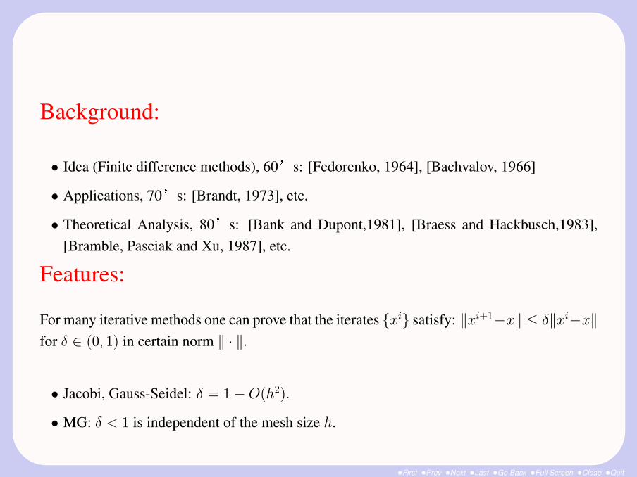
Background:

• Idea (Finite difference methods), 60.s: [Fedorenko, 1964], [Bachvalov, 1966]

• Applications, 70.s: [Brandt, 1973], etc.

• Theoretical Analysis, 80.s: [Bank and Dupont,1981], [Braess and Hackbusch,1983],[Bramble, Pasciak and Xu, 1987], etc.

Features:

For many iterative methods one can prove that the iterates xi satisfy: ‖xi+1−x‖ ≤ δ‖xi−x‖for δ ∈ (0, 1) in certain norm ‖ · ‖.

• Jacobi, Gauss-Seidel: δ = 1−O(h2).

• MG: δ < 1 is independent of the mesh size h.


Observation

Two solution techniques

Iterative method: Jacobi, Gauss-SeidelEasy to perform (matrix × vector), but slow convergence with operations O(N2)

Reason: the higher frequencies of the residual can be supressed quickly, but lower frequenciesare reduced very slowly.

After few iterations, the residual becomes smooth, but not small.

Direct method: Gauss eliminationGood for small-size problemRather difficult to perform for large-size problem, the accuracy is not high (round error accu-mulation)


MGM:Combination of the above two techniquesUsing different techniques on different levels of grid

1. Fine grid (smoothing)

Iterative method–to smooth the residual

2. Coarse grid (correction)

Direct method–to solve the residual equation

3. Add the correction to the initial residual–a more precise residual

4. Back to 1.

Total operations: O(N)


Two types of MGM:

1. W cycle: two corrections per cycle (1980’)

Difficult to carry out, easy to analyze

2. V cycle: one correction per cycle (1990’)

Easy to carry out, difficult to analyze

New schemeCascadic schemeNo correction at all, only iterations on each level.Very easy to carry out, difficult to analyze


Model problem:

The second order elliptic problem−

2∑i,j=1

∂

∂xi(aij

∂u

∂xj) = f in Ω,

u = 0 on ∂Ω,

The differential operator is uniformly elliptic:

cξtξ ≤d∑

i,j=1

aijξiξj ≤ Cξtξ ∀(x, y) ∈ Ω, ξ ∈ Rd.

The variational form: find u ∈ H10(Ω) such that

a(u, v) = (f, v) ∀v ∈ H10(Ω),

where the bilinear form is

a(u, v) =

∫Ω

d∑i,j=1

aij∂u

∂xj

∂v

∂xidx ∀u, v ∈ H1(Ω).


Let Γl (l ≥ 0) denote triangulation of Ω, which is generated uniformly from the initial trian-gulation Γ0. The mesh size is hl = h02

−l. For instance, in 2D case, Γl is obtained by linkingthe midpoints of three edges of triangle or the midpoints of counteredges of rectangle on Γl−1.Let Vl ⊂ L2(Ω) denote the finite element space on Γl. On each level, we define

al(u, v) =∑K∈Γl

∫K

d∑i,j=1

aij∂u

∂xj

∂v

∂xidx

and|v|i,l =

∑K∈Γl

|v|2i,K i = 0, 1,

here ‖v‖0 = |v|0,l.


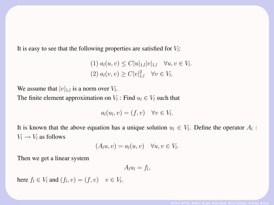
It is easy to see that the following properties are satisfied for Vl:

(1) al(u, v) ≤ C|u|1,l|v|1,l ∀u, v ∈ Vl.

(2) al(v, v) ≥ C|v|21,l ∀v ∈ Vl.

We assume that |v|1,l is a norm over Vl.The finite element approximation on Vl : Find ul ∈ Vl such that

al(ul, v) = (f, v) ∀v ∈ Vl.

It is known that the above equation has a unique solution ul ∈ Vl. Define the operator Al :

Vl → Vl as follows(Alu, v) = al(u, v) ∀u, v ∈ Vl.

Then we get a linear systemAlul = fl,

here fl ∈ Vl and (fl, v) = (f, v) v ∈ Vl.


2. Cascadic Multigrid Method

• Bornemann and Deuflhard (1996)

• Shaidurov (1996)

• Shi and Xu (1998)

• Braess and Dahmen (1999)

• Stevensen (2002)

Advantages:

• Simplicity

• No coarse grid corrections

• One way multigrid


Cascadic Multigrid Algorithm

(1) Set u00 = u∗0=u0 and let

u0l = Ilu

∗l−1.

(2) For l = 1, ..., L, do iterations:uml

l = Cml

l u0l .

(3) Set u∗l =uml

l .

Choose the iterative operator Cl : Vl → Vl on the level l and assume that there exists a linearoperator Tl : Vl → Vl such that ul − Cml

l u0l = Tml

l (ul − u0l ).

Cl : Gauss-Seidel, Jacobi, CG.


Full Multigrid Algorithm


u0l = Ilu

∗l−1.

(2) For l = 1, ..., L, do iterations:

uml

l = MG(l, u0l , r).

(3) Set u∗l =uml

l ,

where MG(l, u0l , r) denotes to do r-th multigrid iterations.

Difference:

No coarse grid corrections in CMG.


Optimal Cascadic Multigrid Method:

If we obtain both the Accuracy

‖uL − u∗L‖L ≈ |u− uL|L

which means that the iterative error is comparable to the approximation error of the

finite element method

and the multigrid Complexity

amount of work = O(nL), nL = dimVL.


Choose the iterative operator Cl : Vl → Vl on the level l and assume that there exists a linearoperator Tl : Vl → Vl such that ul − Cml

l u0l = Tml

l (ul − u0l )

( H2)

(1).‖Tml

l v‖l ≤ Ch−1

l

mγl

|v|t−1,l ∀v ∈ Vl,

(2).‖Tml

l v‖l ≤ ‖v‖l ∀v ∈ Vl,

where ml is the number of iteration steps on the level l, and γ is a positive number dependingon the given iteration.


Introduce a projection operator Pl : Vl−1 + Vl → Vl defined by

al(Plu, v) = al(u, v) ∀v ∈ Vl.

From the definition, it is easily seen that

‖Plv‖l ≤ ‖v‖l−1 ∀v ∈ Vl−1.

For the operator Pl, we assume that(H3)

|v − Plv|t−1,l ≤ Chl|v|t,l−1 ∀v ∈ Vl−1.

Note that the project operator Pl is used only in the convergence analysis, it is not needed inreal computation.


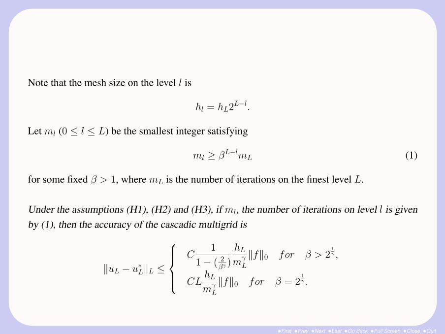
Note that the mesh size on the level l is

hl = hL2L−l.

Let ml (0 ≤ l ≤ L) be the smallest integer satisfying

ml ≥ βL−lmL (1)

for some fixed β > 1, where mL is the number of iterations on the finest level L.

Under the assumptions (H1), (H2) and (H3), if ml, the number of iterations on level l is givenby (1), then the accuracy of the cascadic multigrid is

‖uL − u∗L‖L ≤

C

1

1− ( 2βγ )

hL

mγL

‖f‖0 for β > 21γ ,

CLhL

mγL

‖f‖0 for β = 21γ .


Complexity of CMG:

The computational cost of the cascadic multigrid is proportional to

L∑l=0

mlnl ≤

C1

1− β2d

mLnL for β < 2d,

CLmLnL for β = 2d,

where d is the dimension of the domain Ω.


Main Results:

Suppose (H1), (H2) and (H3) hold.(1) If γ = 1

2, d = 3, then the cascadic multigrid is optimal.(2) If γ = 1, d = 2, 3, then the cascadic multigrid is optimal.(3) If γ = 1

2, d = 2, and the number of iterations on the level L is

mL = [m∗L2],

then the error in the energy norm is

‖uL − u∗L‖L ≤ ChL

m12∗

‖f‖0,

and the complexity is

L∑l=0

mlnl ≤ cm∗nL(1 + lognL)3.

It means that the cascadic multigrid is nearly optimal in this case.


Applications:

1. Lagrange conforming elements

In this case, Vl−1 ⊂ Vl. Therefore, both the transfer operator Il and the projection operator Pl

are the identity I , so that (H1)-1 and (H3) are trivial. By finite element error estimates,

‖ul − Ilul−1‖0 = ‖ul − ul−1‖0 ≤ ‖ul − u‖0 + ‖u− ul−1‖0 ≤ Ch2l ‖f‖0,

so (H1)-2 also holds.

(H2) has been proved by Bank and Dupont (1981)


2. Nonconforming elements

Let Vl be the P1 nonconforming finite element space. Define the intergrid transfer operatorIl : Vl−1 → Vl as follows: let m be the midpoint of a side of triangles in Γl.(1) If m lies in the interior of a triangle in Γl−1, then

(Ilv)(m) := v(m).

(2) If m lies on the common edge of two adjacent triangles T1 and T2 in Γl−1, then

(Ilv)(m) :=1

2(v|T1

(m) + v|T2(m)).

(H1) is valid for the P1 nonconforming element.

Using a duality argument, we can show that (H3) is valid for the P1 nonconforming element.(H2) is obvious.Other nonconforming elements: the Wilson element, the Carey element.


3. The plate bending problem

Let Ω be a convex polygon in R2, the variational form of the plate bending problem is to findu ∈ H2

0(Ω) such thata(u, v) = (f, v) ∀v ∈ H2

0(Ω),

a(u, v) =

∫Ω4u4v + (1− σ)(2

∂2u

∂x1∂x2

∂2v

∂x1∂x2− ∂2u

∂x21

∂2v

∂x22− ∂2u

∂x22

∂2v

∂x21)dx,

(f, v) =

∫Ω

fvdx,

where f ∈ L2(Ω), and 0 < σ < 12 is the Possion ratio. In this case V = H2

0(Ω).


Morley element

The Morley finite element space is nonconforming and nonnested. We define the intergridtransfer operator as follows:

(1) Ilv = 0 at the vertex of Γl along ∂Ω and∂Ilv

∂n= 0 at the midpoint of each edge of Γl along

∂Ω.(2) Let p be a vertex of Γl inside Ω. If p is also a vertex of Γl−1, then (Ilv)(p) = v(p). If p isthe midpoint of a common edge of two triangles K1 and K2 in Γl−1, then

(Ilv)(p) =1

2(v|K1

(p) + v|K2(p)).


(3) Let m be a midpoint of the edge e of Γl inside Ω and n denote the unit normal of e. If m

is inside of a triangle in Γl−1, then

∂Ilv

∂n(m) =

∂v

∂n(m).

If m is on the common edge of two triangles K1 and K2 in Γl−1, then

∂Ilv

∂n(m) =

1

2[∂v|K1

∂n(m) +

∂v|K2

∂n(m)].

We can prove (Shi and Xu 1998)

(H1)-(H3) hold for the Morley element.


3. Economical Cascadic Multigrid Method

Advantages:

• Less operations on the each level.

• Computational costs can be greatly reduced.


Example:

CMG:ml = [mLβL−l] l = 1, · · ·, L,

ECMG:

a new criterion for choosing smoothing steps on each level. When d = 2, that is:

(i) If l > L0, thenml = [mLβL−l].

(ii) If l ≤ L0, thenml = [m

12∗(L− (2− ε0)l)h

−2l ],

here L0 is a positive integer which will be determined later, and 0 < ε0 ≤ 1 is a fixed positivenumber, mL = m0(L− L0)

2. Note that in the standard cascadic algorithm mL = m0L2.


Consider the second order elliptic problem and use Gauss-Seidel iteration as a smoother.For simplicity, we only consider 2D case. Then L0 = L/2 = 4, ε0 = 1

2, h0 = 14, and

m0 = 2, m∗ = 1. The following table shows the iteration steps on each level for the twomethods.

Level 8 7 6 5 4 3 2 1CMG 128 512 2048 8192 32768 131072 524288 2097152

ECMG 32 128 512 2048 1024 896 320 88

We will prove that the new cascadic multigrid algorithm is still optimal in both accuracyand complexity as the standard CMG.


Basic smoothers:

For the basic iterative smoothers, we have

‖Tml

l v‖l ≤ ε(ml, hl)‖v‖0 ∀v ∈ Vl,

where

ε(ml, hl) =

C

h−1l

m12

l

, for ml < κl,

C2−ml

1κl , for ml ≥ κl,

where κl denotes the condition number of the matrix Al.


New criteria for choosing iteration parameters

Determine the largest positive integer L0, which satisfies the following inequality

βL−L0mL ≥ κL0.

For simplicity, we assume that κl = h−2l , then by a simple manipulation,

L0 ≤Llogβ + logmL + 2logh0

logβ + 2log2.

Define the level parameter L0 as the largest positive integer, which satisfies the followinginequality:

L0 ≤ minLlogβ + logmL + 2logh0

logβ + 2log2,

dL

2 + d. (2)


New criteria:

1. When d = 2,


(ii) If l ≤ L0, thenml = [m

12∗(L− (2− ε0)l)κl].

In practical implementation, because κl ≈ h−2l , the above terms can be replaced by:

ml = [m12∗(L− (2− ε0)l)h

−2l ].


2. When d = 3,


(ii) If l ≤ L0, there are two cases:(a) If (2− ε0)L0 ≤ L, then

ml = [m12∗(L− (2− ε0)l)κl].

(b) If(2− ε0)L0 > L, then there exists a largest positive integer L′ < L0 suchthat (2− ε0)L

′ ≤ L. For all l ≤ L′, we choose ml as follows:

ml = [m12∗(L− (2− ε0)l)κl],

for all L′ < l ≤ L0, we choose ml as follows:

ml = [m12∗κl].


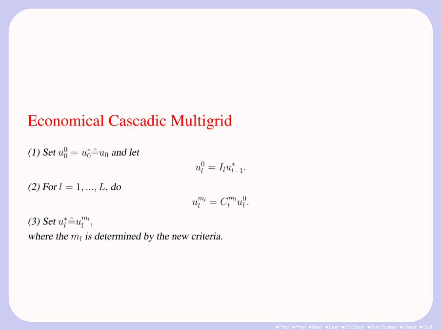
Economical Cascadic Multigrid


u0l = Ilu

∗l−1.

(2) For l = 1, ..., L, douml

l = Cml

l u0l .

(3) Set u∗l =uml

l ,

where the ml is determined by the new criteria.


Main Results:

Suppose (H1) and (H3) hold.(1) If d = 3, then the cascadic multigrid is optimal, i.e.,the error in the energy norm is

‖uL − u∗L‖L ≤ ChL‖f‖0(h0

m12

L

+h0

m12∗

)

and the complexity isL∑

l=0

mlnl ≤ C(h−20 m∗ +

1

1− β2d

mL)nL.


(2) If d = 2, and the number of iterations on the level L is

mL = [m0(L− L0)2],

then the error in the energy norm is


m12∗

+h0

m120

)

and the complexity of computation is

L∑l=0

mlnl ≤ C(m∗h−20 + m0(L− L0)

3)nL.

It means that the cascadic multigrid is nearly optimal in this case.


CG method as a smoother:

Main results:

Suppose (H1) and (H2) hold. For d = 2, 3, the cascadic multigrid with CG smoother isoptimal, i.e., the error in the energy norm is


mL+

h0

m∗)

and the complexity of computation is

L∑l=0

mlnl ≤ C(h−20 +

1

1− β2d

)nL.

It means that the cascadic multigrid is optimal in this case.


Applications:

• Conforming and Nonconforming elements for the second order problem.

• Nonconforming plate elements, Morley element, Adini element.


Numerical experiments:

We use ECMG and standard CMG algorithms to solve the following problem:−4u = f, in Ω = (−1, 1)× (−1, 1),

u = 0, on ∂Ω,

where f is chosen such that the exact solution of the problem is u(x, y) = (1− x2)(1− y2).


ECMG and CMG with GS smoother (P1 conforming element)

CMG ECMGMesh Energy error CPU Energy error CPU

512× 512 7.68851949e-03 38(s) 7.76912806e-03 20(s)1024× 1024 3.82012827e-03 323(s) 3.83635112e-03 101(s)2048× 2048 1.90676237e-03 1420(s) 1.91763892e-03 446(s)


ECMG and CMG with CG smoother (P1 conforming element)


512× 512 7.83833771e-03 14(s) 7.87421203e-03 10(s)1024× 1024 3.95663358e-03 66(s) 3.96542864e-03 42(s)2048× 2048 1.99369401e-03 865(s) 1.99632148e-03 426(s)


ECMG and CMG with GS smoother (P1 nonconforming element)


256× 256 1.18506418e-02 40(s) 1.18713684e-02 19(s)512× 512 5.91793596e-03 294(s) 5.93278651e-03 98(s)

1024× 1024 2.95883706e-03 1382(s) 1.98763892e-03 486(s)


ECMG and CMG with CG smoother (P1 nonconforming element)


256× 256 1.18435038e-02 18(s) 1.18826782e-03 14(s)512× 512 5.91886995e-03 72(s) 5.96752038e-03 48(s)

1024× 1024 2.95842421e-03 447(s) 2.96468190.e-03 310(s)


4. Summary

• Simplicity

• No coarse grid corrections, one way mutigrid

• ECMG: less operations on the each level.

• ECMG: computational costs can be greatly reduced.


5. AppendixEfficiency—Computer vs Algorithm

• Computer1950 → 2000 from 103(Kilo) → 1012(Tera), increase 109(Giga)

• Algorithm (solution of linear system)1950 (Gauss elimination) → 2000 (multigrid method)Convergence rate: from O(N 3) → O(N), increase O(N 2)

• 3D problem: N = (102)3(Mega)

Operations: 1018 → 106, reduce 1012(Tera) !!


THANK YOU!

Email: [email protected], [email protected]

multigrid method - hong kong baptist university · multigrid method zhong-ci shi institute of...

Documents